Feature Learning via Mixtures of DCNNs forFine-Grained Plant Classification

Chris McCool †, ZongYuan Ge †, and Peter Corke †

† Australian Center for Robotic Vision, Queensland University of TechnologyCorresponding author: c.mccool@qut.edu.au or z.ge@qut.edu.au

Abstract. We present the plant classification system submitted by theQUT RV team to the LifeCLEF 2016 plant task. Our system learns twodeep convolutional neural network models. The first is a domain-specificmodel and the second is a mixture of content specific models, one foreach of the plant organs such as branch, leaf, fruit, flower and stem.We combine these two models and experiments on the PlantCLEF2016dataset show that this approach provides an improvement over the base-line system with the mean average precision improving from 0.603 to0.629 on the test set.

Keywords: deep convolutional neural network, plant classification, mix-ture of deep convolutional neural networks

1 Introduction

Fine-grained image classification has received considerable attention recentlywith a particular emphasis on classifying various species of birds, dogs andplants [1, 2, 4, 8]. Fine-grained image classification is a challenging computer vi-sion problem due to the small inter-class variation and large intra-class variation.Plant classification is a particularly important domain because of the implica-tions for automating agriculture as well as enabling robotic agents to detect andmeasure plant distribution and growth.

To evaluate the current performance of the state-of-the-art vision technol-ogy for plant recognition, the Plant Identification Task of the LifeCLEF chal-lenge [5,7] focuses on distinguishing 1000 herb, tree and fern species. This is stillan observation-centered task where several images from seven organs of a plantare related to one observation. There are seven organs, referred to as contenttypes, and include images of the entire plant, branch, leaf, fruit, flower, stem ora leaf scan. In addition to the 1000 known classes, the 2016 PlantCLEF evalu-ation includes classes external to this, making this a more open-set recognitionproblem.

Inspired by [3], we use a deep convolutional neural network (DCNN) approachand learn a separate DCNN for each content type. The DCNN for each contenttype is combined using a mixture of DCNNs. Combining this approach with astandard fine-tuned DCNN improves the mean average precision (mAP) from0.601 to 0.629 on the test set.

2 Our Approach

We propose a system that uses content-types during the training phase, but doesnot use this information at test time. This provides a more practical real-worldsystem that does not require well labelled images from the user. In PlantCLEF2016 there are 7 organ types ranging from branch through to fruit and stem,example images are given in Figure 1.

Our proposed system consists of two key parts. First, we learn a domain-generic DCNN termed φGCNN which classifies the plant image regardless ofcontent type. Second, we learn a MixDCNN termed φMDCNN which first learns acontent specific DCNN for each 6 of the organ types1. We combined the output ofthese two systems to form the final classification decision. For all of our systems,the base network that we use is the GoogLeNet model of Szegedy et al. [9].

Fig. 1. Example images of the 7 organs in the PlantCLEF dataset. From (a)-(g),branch, entire, leaf, leaf scan, flower, fruit, and stem.

2.1 Domain-Generic DCNN

We learn a domain-generic DCNN, φGCNN , that ignores the content type ofthe plant image. This model uses only the class label information to train avery deep neural network consisting of 22 layers, the GoogLeNet model [9]. To

1 The organ type leaf and leaf scan were combined into one.

apply this model to plant data we make use of transfer learning to fine-tune theparameters of this general object classification model to the problem at hand,plant classification.

Transfer learning has been used for a variety fo tasks with one of its earliestuses for fine-grained classification being to learn a bird classification model [10].We use transfer learning to fine-tune the parameters of the GoogLeNet modelby training it for approximately 18 epochs.

2.2 MixDCNN

We learn a MixDCNN, φMDCNN , which consists of K DCNNs. This allowseach of the K DCNNs to learn feature appropriate for those samples that havebeen assigned to it, which in turn allows us to learn more appropriate anddiscrmininative features. We do this by calculating the probability that the k-thcomponent (DCCN), Sk, is responsible for the t-th sample xt. Such an approachalso allows us to have a system that does not require the content type of thesample to be labelled at test time.

For PlantCLEF 2016 there are 7 pre-defined content types consisting of im-ages from the entire plant, branch, leaf, fruit, flower, stem or a leaf scan. For theMixDCNN, we make use of the content type to learn a DCNN that is fine-tuned(specialised) for a subset of the content types. However, because of the similaritybetween the leaf and leaf scan content types we combine them into one. As suchwe learn K = 6 content types for the MixDCNN. To train the k-th component(DCNN) we use the Nk images assigned to this subset Xk = [x1, ...,xNk

], withtheir corresponding class labels. We then fine-tune the GoogLeNet model, simi-lar to Section 2.1, to learn a content-specific model. Once each content-specificDCNN has been trained we then perform joint training using the MixDCNN.

The K trained content-specific models are then combined in a MixDCNNstructure, shown in Figure 2. An important aspect of the MixDCNN model is tocalculate the probability that the k-th component is responsible for the sample.This occupation probability is calculated as,

αk =exp{Ck}∑Kc=1 exp{Cc}

(1)

where Ck is the best classification result for Sk using the t-th sample:

Ck,t = maxn=1...N

zk,n,t (2)

where there are N = 1000 classes and zk,n,t is classification score from the k-thcomponent for the t-th sample and n-th class. This occupation probability giveshigher weight to components that are confident about their prediction.

The final classification score is then given by multiplying the output of thefinal layer from each component by the occupation probability and then summingover the K components:

zn =∑K

k=1zk,nαk (3)

This mixes the network outputs together. More details on this method can befound in [3].

Fig. 2. An overview of the structure of MixDCNN network which consists of K sub-networks that have been trained upon the particular content type.

3 Experiments

In this section we present a comparative performance evaluation of our four runs.We first present the results on the training set and then present the results onthe test set followed by a brief discussion. We use Caffe [6] to learn all of ourmodels, both domain-specific and MixDCNN.

At test time our model does not use any content information, rather it au-tomatically classifies the image with minimal user information. This means weuse all of the 113,205 images of 1,000 classes to train our model. Results on thetraining set are given in Table 1, this table shows the result of the MixDCNNmodel after training for 2 epochs and 17 epochs. The system submitted wastrained for only 2 epochs2 due to resource and time constraints.

Table 1: Top-5 accuracy on the training set and the number of epochs usedfor training the model. The submitted system consisted of the Domain-SpecificModel and MixDCNN-v1.

Method Accuracy Number of Epochs

Domain-Specific Model 80.1% 18MixDCNN-v1 81.0% 2MixDCNN-v2 86.2% 17

2 Further fine-tuning was performed after submission.

3.1 Results on Test Set

In this section, we present our submitted results for the PlantCLEF2016 chal-lenge. We submitted four runs:

– QUT Run 1 is the Baseline result of using a fine-tuned GoogLeNet using allof the organ types, the rank 1 score submitted for each observation.

– QUT Run 2 is the MixDCNN system with the rank 1 score submitted foreach observation.

– QUT Run 3 is the combination of the Baseline and MixDCNN systems, therank 1 score was submitted for each observation.

– QUT Run 4 is the combiation of the Baseline and MixDCNN system with athreshold to remove potential false positives.

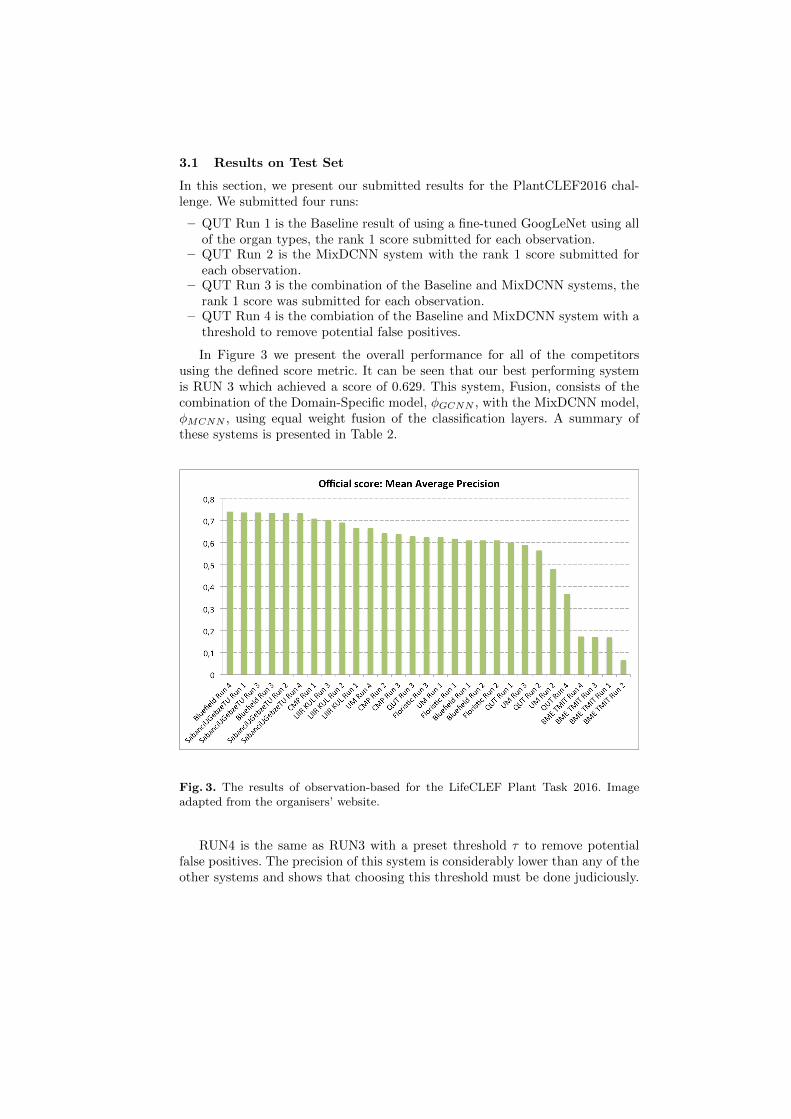
In Figure 3 we present the overall performance for all of the competitorsusing the defined score metric. It can be seen that our best performing systemis RUN 3 which achieved a score of 0.629. This system, Fusion, consists of thecombination of the Domain-Specific model, φGCNN , with the MixDCNN model,φMCNN , using equal weight fusion of the classification layers. A summary ofthese systems is presented in Table 2.

Fig. 3. The results of observation-based for the LifeCLEF Plant Task 2016. Imageadapted from the organisers’ website.

RUN4 is the same as RUN3 with a preset threshold τ to remove potentialfalse positives. The precision of this system is considerably lower than any of theother systems and shows that choosing this threshold must be done judiciously.

Table 2: Mean average precision on the test set for the submitted models.Method Accuracy Number of Epochs

Domain-Specific Model (RUN1) 0.603 18MixDCNN-v1 (RUN2) 0.564 2Fusion (RUN3) 0.629 N/AFusion with threshold (RUN4) 0.367 N/A

4 Conclusions and Future Work

In this paper we presented a domain-specific and MixDCNN model to performautomatic classification of plant images. The domain-specific model is learnt byfine-tuning a well known model specifically for the plant classification task. TheMixDCNN model is learnt by first fine-tuning a model to K subsets of data,in this case by using different organ types. We then jointly optimise these KDCNN models by using the mixture of DCNNs framework. Combining thesetwo approaches yields improved performance and demonstrates the importanceof learning complementary models to perform accurate classification with theperformance improving from 0.603 to 0.629. We note that the MixDCNN modelwas only trained for 2 epochs we expect improved performance with a modelwhich has been trained for longer. Finally, this system is fully automatic as itdoes not require the organ (content) type to be specified at test time.

Acknowledgements

The Australian Centre for Robotic Vision is supported by the Australian Research

Council via the Centre of Excellence program.

References

1. Y. Chai, V. Lempitsky, and A. Zisserman. Symbiotic segmentation and part local-ization for fine-grained categorization. In ICCV, 2013.

2. Efstratios Gavves, Basura Fernando, Cees GM Snoek, Arnold WM Smeulders, andTinne Tuytelaars. Local alignments for fine-grained categorization. InternationalJournal of Computer Vision, pages 1–22, 2014.

3. ZongYuan Ge, Alex Bewley, Christopher McCool, Ben Upcroft, Conrad Sanderson,and Peter Corke. Fine-grained classification via mixture of deep convolutionalneural networks. WACV, 2016.

4. ZongYuan Ge, Christopher McCool, Conrad Sanderson, and Peter Corke. Subsetfeature learning for fine-grained classification. CVPR Workshop on Deep Vision,2015.

5. Herve Goeau, Pierre Bonnet, and Alexis Joly. Plant identification in an open-world(lifeclef 2016). In CLEF working notes 2016, 2016.

6. Yangqing Jia, Evan Shelhamer, Jeff Donahue, Sergey Karayev, Jonathan Long,Ross Girshick, Sergio Guadarrama, and Trevor Darrell. Caffe: Convolutional ar-chitecture for fast feature embedding. arXiv:1408.5093, 2014.

7. Joly, Alexis and Goeau, Herve and Glotin, Herve and Spampinato, Concetto andBonnet, Pierre and Vellinga , Willem-Pier and Champ, Julien and Planque, Robertand Palazzo, Simone and Muller, Henning. Lifeclef 2016: multimedia life speciesidentification challenges. In Proceedings of CLEF 2016, 2016.

8. Asma Rejeb Sfar, Nozha Boujemaa, and Donald Geman. Confidence sets for fine-grained categorization and plant species identification. IJCV, 2014.

9. Christian Szegedy, Wei Liu, Yangqing Jia, Pierre Sermanet, Scott Reed, DragomirAnguelov, Dumitru Erhan, Vincent Vanhoucke, and Andrew Rabinovich. Goingdeeper with convolutions. arXiv:1409.4842, 2014.

10. Ning Zhang, Jeff Donahue, Ross Girshick, and Trevor Darrell. Part-based R-CNNsfor fine-grained category detection. In ECCV, pages 834–849. 2014.