Feb 2007 Big Sky, Montana Nuclear Dynamics 2007 Conference Is There A Mach Cone? For the STAR Collaboration Claude Pruneau Motivations/Goals Expectations/Models

QuickTime™ and aTIFF (Uncompressed) decompressor

are needed to see this picture.

Feb 2007 Big Sky, Montana

Nuclear Dynamics 2007 Conference

Is There A Mach Cone?For the STAR Collaboration

Claude Pruneau

Motivations/Goals Expectations/Models

Search + Analysis Methods Data + Results

Summary/Conclusions



Claude Pruneau, for the STAR Collaboration, Nucl. Dyn 2007 2QuickTime™ and a

TIFF (Uncompressed) decompressorare needed to see this picture.

Dip “Puzzle” Dip “Puzzle” in in 2-Particle Correlations

pTtrig = 3.0-4.0 GeV/c;

pTasso = 1.0-2.5 GeV/c

See M. Horner’s talk at QM06

Motivations Mach Cone Concept/Calculations

Stoecker, Casalderry-Solana et al, Muller et al.; Ruppert et al., …

Velocity Field Mach Cone

Other Scenarios• Cherenkov Radiation

Dremmer, Majumder, Koch, & Wang; Vitev• Jet Deflection (Flow) Fries; Armesto et al.; Hwa

vs~0.33

~1.1 rad

θM = π ± arccos(vs / c)

~ 1.9, 4.3rad



Relative Angles Definition

1

2

3

12

13

Angular Range 0 - 360o

1: 3 < pt < 4 GeV/c (Jet Tag)2,3: 1 < pt < 2 GeV/c,

Mach Cone & Deflection Kinematical Signatures

13

12

0

Back-to-back Jets “in vacuum”Away-side broadeningAway-side deflection & flowMach Cone



Two Analysis Techniques

ρ2 (Δϕ ij ) ≡d 2N

dΔϕ ij

Measure 1-, 2-, and 3-Particle Densities

3-particle densities = superpositions of truly correlated 3-particles, and combinatorial components. We use two approaches to extract the truly correlated 3-particles component

ρ1(ϕ i ) ≡d 2N

dϕ iρ3(Δϕ ij , Δϕ ik ) ≡

d 3N

dΔϕ ijdΔϕ ik

C3( 1 , 13) =ρ3( 1 , 13)−ρ ( 1 )ρ1(3)−ρ ( 13)ρ1()−ρ ( 13 − 1 )ρ1(1) + ρ1(1)ρ1()ρ1(3)

1) Cumulant technique: 2) Jet+Flow Subtraction Model:

J3( 1 , 13) =J 3( 1 , 13)−J ( 1 )B ( 13)

−J ( 13)B ( 1 )−B3( 1 , 13)

Simple DefinitionModel Independent.

Intuitive in conceptSimple interpretation in principle.

PROs

CONs Not positive definiteInterpretation perhaps difficult.

Model Dependentv2 and normalization factors systematics

–.

See C. Pruneau, nucl-ex/0608002 See J. Ulery & nucl-ex/0609017/0609016



Mach Cone Search - Data set and cuts

• p+p, d+Au, = 200 GeV used as reference.

• Search For Mach Cone in Au + Au, = 200 GeV

• Minimum bias, and Central Triggers Data Samples (Run 4)

• Particle Cuts: Predicated by the observation of the “dip”• Jet tag (trigger) : 3 < pt < 4 GeV/c, ||<1• Associates: 1 < pt < 2 GeV/c, ||<1

• Collision Centrality: • Estimated based on reference multiplicity in || < 0.5.

s

s



ρ3(Δϕ 12 ,Δϕ 13) ρ2 (12)ρ1(3) ρ2 (13)ρ1(2)

Measurement of 3-Particle Cumulant

ρ2 (23)ρ1(1) v2v2v4

• Clear evidence for finite 3-Part Correlations• Observation of flow like and jet like structures.

• Evidence for v2v2v4 contributions

C3( 1 , 13)



3-Cumulant vs. centralityAu + Au 80-50% 30-10% 10-0%





3-Cumulant Sensitivity to Cone Signal

Use a simple Jet + Cone toy modelJet: <N1>=1 per jet (3<pt<4 GeV/c)<N2>=2 per jet (1<pt<2 GeV/c)<Jet>/event ~ 0.27Actual data have ~1 trigger/event

Cone: <N2>=2 per jet (1<pt<2 GeV/c)

Event Mult ~ 300 to 600.

C3( 1 , 13)

Cone

Near SideJet



C3( i , j , k)FJ ≈( )−1 J AiAj Bk

×v ( jet)v (bckg)exp(−σ )exp − ij

4σ

⎛⎝⎜

⎞⎠⎟cos k − i − j( )

3-Cumulant Background: Jet x Flow

Flowing Jet - Differential Attn. Rel. Reaction PlaneModel:Jet Emission Rel. Reaction Plane with Finite v2.2 particles from a jet 1 particle from the background

C3( 1 , 13)

(a.u.)

Work in progress to assess the strength of this term in the cumulant and systematics.



Jet-Flow Subtraction Method

See J. Ulery, nucl-ex/0609017/0609016

Δ12

Δ 1

3

ρ3(Δϕ 12 , Δϕ 13) / Trigger

Δ12

2-Part Correlation

Flow background

“Jetty”signal

Δ12

Δ 1

3

Estimate/Remove JetBackground Hard-Soft Term



Estimate/Remove Trigger 2-Background Soft-soft term

Δ 1

3

Δ12

Jet-Flow Subtraction Method (cont’d)Estimate/Remove Trigger Background Flow

v2(1) v2(2) v22

v4 (1) v4 (2) + +v2(1)v2(2)v2(3) v2

4

Δ 1

3

Δ12

Δ 1

3

Δ12

v4=1.15v22



Jet - Flow Subtraction Method - System Size Dependence (1)

(12+13)/2-

(12-13)/2

Δ12 Δ12 Δ12

Δ 1

3

Δ 1

3

Δ 1

3

pp d+AuAu+Au 50-80%



Jet - Flow Subtraction Method - System Size Dependence (1)

Δ 1

3

Δ 1

3

Δ 1

3

Δ12Δ12

Δ12

(12+13)/2-

(12-13)/2

Au+Au 30-50% Au+Au 10-30% Au+Au 0-10%



12

1

3Jet - Flow Subtraction Result in Au+Au - Triggered 0-12%

Diagonal and Off-diagonal structures are suggestive of conical emission at an angle of about 1.45 radians in central Au+Au.

Deflected Jet + Cone

Cone

Near Side

Elongated Away Side Jet



Yield and SystematicsAu+Au 0-12% No Jet Flow

12

1

3

(12+13)/2-

(12-13)/2

Au+Au 0-12%

12

(12-13)/2

(12+13)/2-

1

3

Nominal Model:• Used “reaction plane” v2 estimates• Used Zero Yield at 1 rad for

normalizations

“Systematics” Estimates:• Vary v2 in range: v2{2} - v2{4}• Vary point of normalization

Turn Jet-Flow background term on/off



• Use 3 Particle Azimuthal Correlations.• Identification of correlated 3-particle from jet and predicted Mach

cone is challenging task.• Must eliminate 2-particle correlation combinatorial terms.• Must remove flow background - including v2v2, v4v4, and v2v2v4

contributions.• Use two approaches: Cumulant & Jet - Flow Subtraction Model

• Cumulant Method• Unambiguous evidence for three particle correlations.• Clear indication of away-side elongated peak.• No evidence for Cone signal given flow backgrounds

• Jet-Flow Background Method• Model Dependent Analysis

• Cone amplitude sensitive to magnitude v2 and details of the model.

• Observe Structures Consistent with Conical emission in central collisions

Summary/Conclusions



Additional Material



Azimuthal FlowPF ( i |ψ ) =1+ vm

m∑ (i)cos m i −ψ( )( )

ρ,F ( i , j ) = ( )− FiFj − Fi Fj + FiFj vm(i)vm( j)cos m i − j( )( )m∑⎛

⎝⎜⎞⎠⎟

Particle Distribution Relative to Reaction Plane

2- Cumulants

ρ3,F ( i , j , k) = ( )−3

FiFjFk − FiFj Fk( ) vm(i)vm( j)cos m i − j( )( )m∑

+permutations (j,k,i) and (k,i,j) of above

FiFjFk vp(i)vm( j)vn(k)

δ p,m+n cos p i −m j −n k( )

+δm,p+n cos −p i + m j −n k( )

+δn,m+k cos −p i −m j +n k( )

⎡

⎣

⎢⎢⎢⎢

⎤

⎦

⎥⎥⎥⎥

p,m,n∑

−constant terms

⎧

⎨

⎪⎪⎪⎪⎪

⎩

⎪⎪⎪⎪⎪

⎫

⎬

⎪⎪⎪⎪⎪

⎭

⎪⎪⎪⎪⎪

Reducible2nd order in v

Irreducible3rd order in v

3- Cumulants

• 3-Cumulant Flow Dependence : • Irreducible v2v2v4 contributions

• Must be modeled and manually subtracted• v2

2 suppressed but finite• v2

2 cancellation possible with modified cumulant.



Two Illustrative Models :

σ1= σ2= σ3=10o; σ=0o

No deflection Random Gaussian Away-Side Deflectionσ1= σ2= σ3=10o; σ=30o

Di-Jets:


are needed to see this picture.QuickTime™ and aTIFF (Uncompressed) decompressor


Mach Cone

θmach

(a)

12

13

θ mach

(b)

θ mach



Some Properties of CumulantsCumulants are not positive definiteThe number of particles in a bin varies e-by-e: ni = <ni> + i

n1n2 = n1 + 1( ) n + ( ) = n1 n + 1

n1n2n3 = n1 + 1( ) n + ( ) n3 + 3( )

= n1 n n3 + n1 3 + n 13 + n3 1 + 1 C3 = 1

Cumulant for Poisson Processes (independent variables) are null

C2 = n1n − n1 n = 1 =0 C3 = 1 =0

Cumulant for Bi-/Multi-nomial Processes ~ 1/Mn-1

(independent variables, but finite multiplicity)

n1 =p1M

n =pM

Var(n1) = n1 − n1

=p1(1−p1)M

n1n =p1pM

Where M is a reference multiplicity

C2 = n1n − n1 n = 1

n1n2 − n1 n

n1 n

=−1M



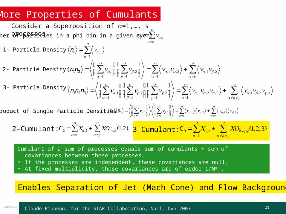
More Properties of CumulantsConsider a Superposition of =1,…, s processes

Number of particles in a phi bin in a given event: ni = n,i=1

s

∑1- Particle Density: ni = n,i

=1

s

∑

2- Particle Density: n1n2 = n ,1=1

s

∑⎛⎝⎜⎞⎠⎟

nβ,β=1

s

∑⎛

⎝⎜⎞

⎠⎟= n ,1n ,

=1

s

∑ + n ,1nβ,≠β

s

∑

Product of Single Particle Densities: n1 n2 = n ,1=1

s

∑⎛⎝⎜⎞⎠⎟

nβ,β=1

s

∑⎛

⎝⎜⎞

⎠⎟= n ,1 n ,

=1

s

∑ + n ,1 nβ,≠β

s

∑

2-Cumulant: C2 = C,=1

s

∑ + COVβ (1,)≠β

s

∑

Cumulant of a sum of processes equals sum of cumulants + sum of covariances between these processes.

• If the processes are independent, these covariances are null.• At fixed multiplicity, these covariances are of order 1/Mn-1.

3- Particle Density: n1n2n3 = n ,1=1

s

∑⎛⎝⎜⎞⎠⎟

nβ,β=1

s

∑⎛

⎝⎜⎞

⎠⎟nγ,

γ=1

s

∑⎛

⎝⎜⎞

⎠⎟= n ,1n ,n ,3

=1

s

∑ + n ,1nβ,nγ,3≠β≠γ

s

∑

3-Cumulant: C3 = C,3=1

s

∑ + COVβγ (1,,3)≠β≠γ

s

∑

Enables Separation of Jet (Mach Cone) and Flow Background.



Example: 2-particle Decay: ρ → + + −

2-Cumulant

Maxwell Boltzman, T=0.2 GeVIsotropic Emission/Decay of rho-mesons, with pion background.

• 3-Particle Density contains 2-body decay signals.• 2-Body Signal Not Present in 3-cumulant.

Suppression of 2-part correlations with 3-cumulant

Many resonances, e.g. ρ 0

s , N*, … contribute to the soft-soft term, and likely to the hard-soft as well.



Cumulant Method - Finite Efficiency Correction

• Use “singles” normalization to account for finite and non-uniform detection efficiencies.

• Example: ρ2 (Δϕ ij )

ρ1ρ1(Δϕ ij )=

ρ2 (Δϕ ij )

ρ1(ϕ i )ρ1(ϕ j )δ (Δϕ ij −ϕ i +ϕ j )∫Robust Observables

ρ2 (Δϕ ij )

ρ1ρ1(Δϕ ij )

Measured

=ε 2 (ϕ i ,ϕ j )ρ 2

theory (ϕ i ,ϕ j )

ε1(ϕ i )ρ 1

theory (ϕ i )ε1(ϕ j )ρ 1

theory (ϕ j )δ (Δϕ ij −ϕ i +ϕ j )dϕ idϕ j∫

=ρ

2

theory (ϕ i ,ϕ j )

ρ1

theory (ϕ i )ρ 1

theory (ϕ j )δ (Δϕ ij −ϕ i +ϕ j )dϕ idϕ j∫

provided

ε 2 (ϕ i ,ϕ j ) = ε1(ϕ i )ε1(ϕ j ) verified for sufficiently large ij differences.



What changed since QM05

Background subtractedQM2005

Au+Au 0-10% most central

Example Acceptance Correction• Increased data sample• Two Analysis Methods• Jet-Flow Background Method:

• Improved efficiency corrections• Reduce the number of free parameters



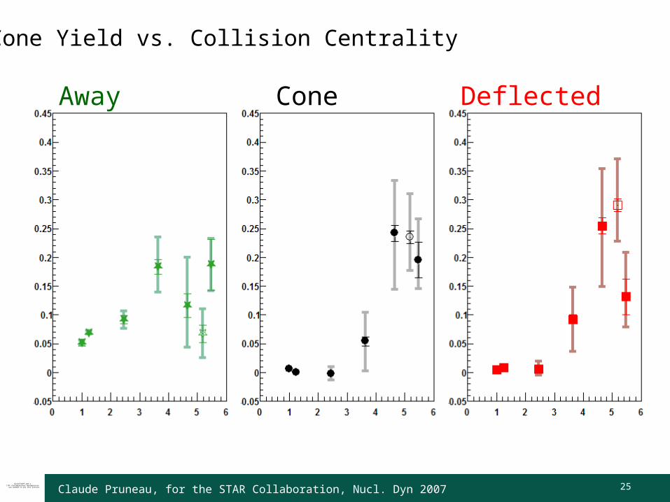
Away Cone Deflected

Cone Yield vs. Collision Centrality

Documents

Feb 2007 Big Sky, Montana Nuclear Dynamics 2007 Conference Is There A Mach Cone? For the STAR Collaboration Claude Pruneau Motivations/Goals Expectations/Models