February 17, 2015Applied Discrete Mathematics Week 3: Algorithms 1 Double Summations Table 2 in 4 th Edition: Section 1.7 5 th Edition: Section 3.2 6 th

February 17, 2015 Applied Discrete Mathematics Week 3: Algorithms

1

Double Summations

Table 2 in

4th Edition: Section 1.7

5th Edition: Section 3.2

6th and 7th Edition: Section 2.4

contains some very useful formulas for calculating sums.

In the same Section, Exercises 15 and 17 (7th Edition: Exercises 31 and 33) make a nice homework.


2

Enough Mathematical Appetizers!

Let us look at something more interesting:

Algorithms


3

Algorithms

What is an algorithm?

An algorithm is a finite set of precise instructions for performing a computation or for solving a problem.

This is a rather vague definition. You will get to know a more precise and mathematically useful definition when you attend CS420 or CS620.

But this one is good enough for now…


4

Algorithms

Properties of algorithms:

• Input from a specified set,• Output from a specified set (solution),• Definiteness of every step in the computation,• Correctness of output for every possible input,• Finiteness of the number of calculation steps,• Effectiveness of each calculation step and• Generality for a class of problems.


5

Algorithm Examples

We will use a pseudocode to specify algorithms, which slightly reminds us of Basic and Pascal.

Example: an algorithm that finds the maximum element in a finite sequence

procedure max(a1, a2, …, an: integers)max := a1

for i := 2 to nif max < ai then max := ai

{max is the largest element}


6

Algorithm Examples

Another example: a linear search algorithm, that is, an algorithm that linearly searches a sequence for a particular element.

procedure linear_search(x: integer; a1, a2, …, an: integers)

i := 1while (i n and x ai)

i := i + 1if i n then location := ielse location := 0{location is the subscript of the term that equals x, or is zero if x is not found}


7

Algorithm Examples

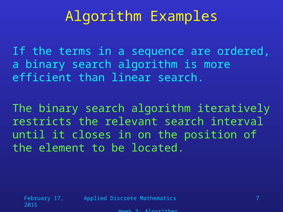
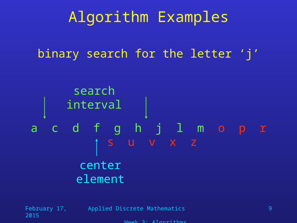
If the terms in a sequence are ordered, a binary search algorithm is more efficient than linear search.

The binary search algorithm iteratively restricts the relevant search interval until it closes in on the position of the element to be located.


8

Algorithm Examples

a c d f g h j l m o p r s u v x z

binary search for the letter ‘j’

center element

search interval


9

Algorithm Examples



center element

search interval


10

Algorithm Examples



center element

search interval


11

Algorithm Examples



center element

search interval


12

Algorithm Examples



center element

search interval

found !


13

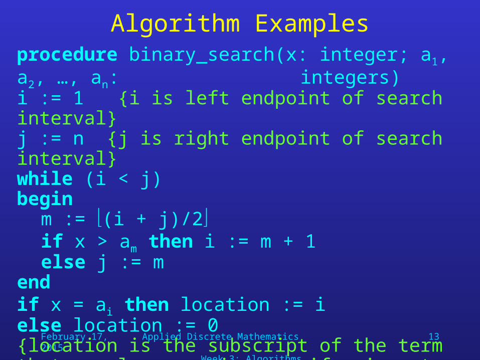
Algorithm Examplesprocedure binary_search(x: integer; a1, a2, …, an:

integers)i := 1 {i is left endpoint of search interval}j := n {j is right endpoint of search interval} while (i < j)begin

m := (i + j)/2if x > am then i := m + 1else j := m

endif x = ai then location := ielse location := 0{location is the subscript of the term that equals x, or is zero if x is not found}


14

Algorithm Examples

Obviously, on sorted sequences, binary search is more efficient than linear search.

How can we analyze the efficiency of algorithms?

We can measure the • time (number of elementary computations) and• space (number of memory cells) that the algorithm requires.

These measures are called computational complexity and space complexity, respectively.


15

Complexity

What is the time complexity of the linear search algorithm?

We will determine the worst-case number of comparisons as a function of the number n of terms in the sequence.

The worst case for the linear algorithm occurs when the element to be located is not included in the sequence.

In that case, every item in the sequence is compared to the element to be located.


16

Algorithm Examples

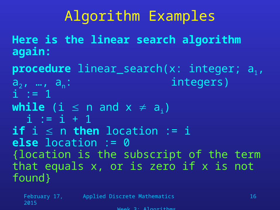
Here is the linear search algorithm again:

procedure linear_search(x: integer; a1, a2, …, an: integers)

i := 1while (i n and x ai)

i := i + 1if i n then location := ielse location := 0{location is the subscript of the term that equals x, or is zero if x is not found}


17

Complexity

For n elements, the loop

while (i n and x ai)i := i + 1

is processed n times, requiring 2n comparisons.

When it is entered for the (n+1)th time, only the comparison i n is executed and terminates the loop.

Finally, the comparison if i n then location := iis executed, so all in all we have a worst-case time complexity of 2n + 2.


18

Reminder: Binary Search Algorithmprocedure binary_search(x: integer; a1, a2, …, an:

integers)i := 1 {i is left endpoint of search interval}j := n {j is right endpoint of search interval} while (i < j)begin


endif x = ai then location := ielse location := 0{location is the subscript of the term that equals x, or is zero if x is not found}


19

Complexity

What is the time complexity of the binary search algorithm?

Again, we will determine the worst-case number of comparisons as a function of the number n of terms in the sequence.

Let us assume there are n = 2k elements in the list, which means that k = log n.

If n is not a power of 2, it can be considered part of a larger list, where 2k < n < 2k+1.


20

Complexity

In the first cycle of the loop

while (i < j)begin


end

the search interval is restricted to 2k-1 elements, using two comparisons.


21

Complexity

In the second cycle, the search interval is restricted to 2k-2 elements, again using two comparisons.

This is repeated until there is only one (20) element left in the search interval.

At this point 2k comparisons have been conducted.


22

Complexity

Then, the comparison

while (i < j)

exits the loop, and a final comparison

if x = ai then location := i

determines whether the element was found.

Therefore, the overall time complexity of the binary search algorithm is 2k + 2 = 2 log n + 2.


23

Complexity

In general, we are not so much interested in the time and space complexity for small inputs.

For example, while the difference in time complexity between linear and binary search is meaningless for a sequence with n = 10, it is gigantic for n = 230.


24

Complexity

For example, let us assume two algorithms A and B that solve the same class of problems.

The time complexity of A is 5,000n, the one for B is 1.1n for an input with n elements.


25

Complexity

Comparison: time complexity of algorithms A and B

Algorithm A Algorithm BInput Size

n

10

100

1,000

1,000,000

5,000n

50,000

500,000

5,000,000

5109

1.1n3

2.51041

13,781

4.81041392


26

Complexity

This means that algorithm B cannot be used for large inputs, while running algorithm A is still feasible.

So what is important is the growth of the complexity functions.

The growth of time and space complexity with increasing input size n is a suitable measure for the comparison of algorithms.


27

The Growth of Functions

The growth of functions is usually described using the big-O notation.

Definition: Let f and g be functions from the integers or the real numbers to the real numbers.We say that f(x) is O(g(x)) if there are constants C and k such that

|f(x)| C|g(x)|

whenever x > k.


28


When we analyze the growth of complexity functions, f(x) and g(x) are always positive.

Therefore, we can simplify the big-O requirement to

f(x) Cg(x) whenever x > k.

If we want to show that f(x) is O(g(x)), we only need to find one pair (C, k) (which is never unique).


29


The idea behind the big-O notation is to establish an upper boundary for the growth of a function f(x) for large x.

This boundary is specified by a function g(x) that is usually much simpler than f(x).

We accept the constant C in the requirement

f(x) Cg(x) whenever x > k,

because C does not grow with x.

We are only interested in large x, so it is OK iff(x) > Cg(x) for x k.


30


Example:

Show that f(x) = x2 + 2x + 1 is O(x2).

For x > 1 we have:

x2 + 2x + 1 x2 + 2x2 + x2

x2 + 2x + 1 4x2

Therefore, for C = 4 and k = 1:

f(x) Cx2 whenever x > k.

f(x) is O(x2).

Documents

February 17, 2015Applied Discrete Mathematics Week 3: Algorithms 1 Double Summations Table 2 in 4 th Edition: Section 1.7 5 th Edition: Section 3.2 6 th