Feedback complexity, bounded rationality,and market dynamics

Christian Kampmann John D. Sterman*

Department of Physics, Bldg. 309 Sloan School of Management, E53-351Technical University of Denmark Massachusetts Institute of Technology

2800 Lyngby, Denmark Cambridge, MA 02142cek@chaos.fys.dtu.dk jsterman@mit.edu

ABSTRACT

In a set of experimental markets we investigate how the dynamic structure of an economyinteracts with different price-setting institutions to determine market performance, stabilityand learning. We test the standard assumptions of optimality and rational expectationsagainst a behavioral hypothesis in which subjects ignore critical elements of the feedbackstructure in which they operate (‘misperceptions of feedback’).

We find first that the introduction of even modest levels of dynamic complexity to thestructure of the experimental economy significantly and substantially degradesperformance relative to optimal, supporting the behavioral hypotheses. In the dynamicallycomplex conditions, subjects generate costly, systematic fluctuations in prices andquantities. The institutional structure of the market also has a strong effect onperformance relative to optimal. Performance is improved, but remains significantlybelow, optimal in the presence of market institutions, even in the case of a perfectlyfunctioning market with computer-mediated market clearing. Markets moderate but donot eliminate the negative impact of bounded rationality and poor mental models.

We then analyze the decisions of individual subjects by fitting them to various models ofdecision making. The estimates reject the hypothesis of rationality at the individual level.We then simulate the markets using the estimated decision rules. The simulationsreproduce the most salient features of the dynamics, and variations between markets arerelated to differences the parameters values of the decision rules which characterize thedegree to which subjects misunderstand the feedback structure of the market. In thismanner, the analysis links microstructure to macrobehavior, coupling observation ofindividual decision making behavior and the genesis of aggregate market outcomes.

Decision timing data and verbal protocols provide evidence that increasing complexity ofthe decision-making task leads subjects to ignore important aspects of the decisionenvironment, particularly strategic interactions. In the face of dynamic complexity,subjects revert to simple, reactive decision rules, rules which prove to be dysfunctional.Moreover, subjects tend to attribute the oscillations and other systematic dynamics theyexperience to exogenous shocks rather than to their own interactions with the system.This latter phenomenon may have important implications for the ability of agents to learnand improve their behavior over time.

* Corresponding author. Version of June 1998. Comments welcomed.

2

1. Introduction

The standard neoclassical assumptions of rational, optimizing agents with unbiasedexpectations stand in sharp contrast to evidence from psychological studies of biases anderrors in human decision making (see e.g. Conlisk 1996 and Hogarth and Reder 1987 foroverviews). The contrast has become stronger over the years, as modern dynamiceconomic theories employ increasingly sophisticated methods of optimal filtering andcontrol (Arrow 1987, Sargent 1993) while behavioral scientists continue to accumulateevidence of human shortcomings in such tasks. In particular, a number of recent studiesshow that decision making in complex dynamic environments is poor relative tonormative standards, or even simple decision rules, especially when decisions haveindirect, delayed, nonlinear, and multiple feedback effects (e.g., Brehmer 1992, Diehl andSterman 1995, Funke 1991, Kleinmuntz 1985, Paich and Sterman 1993, Smith et al.1988, Sterman 1989a, b).

It is widely argued that any departures from rationality will be short-lived in real marketsdue to processes of market adjustment through arbitrage, adaptation, learning and, in thelonger run, through competitive selection. As Conlisk (1996), among others, argues,these claims must be examined explicitly to determine where neoclassical approachesmight be sufficient and where other theories are called for. Moreover, such studies mustbe rooted in observations of human decision making, both in the laboratory and the field.

Bounded rationality and systematic errors in dynamic decision making are important forseveral reasons, even when these phenomena are shown to occur in contexts whereeconomic forces are absent. There are many dynamic decision making tasks in the realworld for which no or only poorly functioning markets exist, including real-time processcontrol, organizational settings such as bureaucracies (both corporate and governmental),environmental dynamics, etc. In the subset of cases where various market institutionsexist, the ability of market forces to mitigate individual departures from rationality indynamic tasks cannot be assumed, but must be subjected to empirical test. In cases wheremarket forces do not eliminate misperceptions of feedback, one must search foralternatives to the neoclassical assumptions of perfect rationality and equilibrium toprovide an explicit theory of disequilibrium market processes, based on assumptionsabout individual behavior that accord with observed human decision making.

Accordingly, the research questions addressed in the present study are: (1) To whatextent can market mechanisms and financial incentives alleviate the problems observed innon-market dynamic decision making experiments? (2) What is the effect of feedbackcomplexity on market behavior and performance? (3) Can one explain aggregate marketbehavior from the individual decision-making behavior?

We study these questions in a set of six experimental markets, varying both the feedbackcomplexity and the market institution, as explained in the next section. In Section 3, wecompare aggregate performance and stability to optimal performance across theconditions, and in Section 4, we demonstrate how salient features of the macro-levelexperimental outcomes can be explained by a set of simple decision heuristics at themicro-level of individual agents. In Section 5, we examine timing data and questionnaire

3

responses to gain further insight into how subjects cope with varying task characteristics.Our conclusions and comments are found in Section 6.

2. Experimental design and method

2.1. Experimental treatments

The study follows standard procedures in experimental economics, such as performance-based cash rewards to the participants, single-individual agents (firms), discrete timeperiods, and no verbal communication between subjects. However, one importantdifference is the dynamic structure of the market. Most studies in experimentaleconomics involve markets with relatively simple dynamic structure. In particular,markets are often reinitialized each period so that no inventories of unsold goods orbacklogs of unfilled orders carry over to future periods, unlike most real-world situations.In this manner, markets are "reset" each period (Plott 1982, Smith 1982). In suchsettings, the current decisions of the agents are conditioned by outcome feedback frompast experience, but the structure of the task and states of the system are not affected bypast decisions. These conditions enable learning to occur because agents gain experiencefrom repeated ‘rounds’ of ‘play’ in an unchanging situation . In real situations, however,decisions have another effect: they alter the state of the system in ways that change thedecision environment faced in the future. This action feedback means that even as peopleattempt to learn from past experience, their own actions, interacting with the physics of thesystem and the decisions of other agents, feed back to change the system in which theyare embedded, possibly rendering any learning from experience obsolete or even harmful.Experimental studies show that human performance can degrade significantly in dynamicdecision-making tasks involving action feedback, particularly in the presence of delays,accumulations (stocks and flows), non-linearities, and self-reinforcing (positive) feedback(Diehl and Sterman 1995, Paich and Sterman 1993, Sterman 1989a, b). Thus, theexperimental markets in this study involved two feedback complexity conditions:

• A simple condition, where production initiated at the beginning of eachperiod becomes available for storage or delivery during that same period, andwhere industry demand is unaffected by the average level of activity in themarket;

• A complex condition, where there is a lag between the time production isinitiated and the time it becomes available for storage or delivery, and whereindustry demand is influenced by average market production, representing amultiplier effect from income to aggregate demand.

Experimental studies in economics, even without dynamic complexity, have long shownthat the institutional structure of the market influences the convergence to and nature ofequilibrium (Plott 1986, Smith 1986). Double auctions typically converge rapidly andreliably to competitive equilibrium. Posted price systems, where agents announce buyingor selling prices, converge more slowly and often do not reach competitive equilibrium.Our experiments thus involved three price-setting institutions:

4

• Fixed prices: All prices are completely fixed and equal. Fluctuations indemand are accommodated entirely by changes in inventories. (All firmsreceive an equal share of market demand.)

• Posted seller prices: Each firm sets its own price and production rate, anddemand is fully accommodated by changes in inventories.

• Clearing prices: Prices move to equate demand to the given supply eachperiod. In this condition, the need for inventories is eliminated. The market-clearing price vector, given the current period's output vector and demandfunction, is found by the computer.

We combined the two feedback complexity conditions and three price setting conditionsinto a between-subjects design with six experimental conditions. Each subject would playonly once. The experiment involved four markets in each treatment condition, for a totalof 24, and with a total of 97 subjects.

2.2. Market structure

The market consists of K firms (operated by experimental subjects) and a consumersector (modeled by the computer). The market can be interpreted as a regional industrywhere the level of activity and employment may influence aggregate demand in the region.Following standard models of monopolistic competition, the products of the industryhave some limited degree of differentiation (the firm demand elasticity is large but finite)but the market is otherwise close to the perfect-competition ideal.

Time is divided into discrete periods. At the beginning of each period t , each firm idecides how much production yi,t to initiate and, in the posted-price condition, what pricepi, t to charge for its product. Firms make these decisions ex ante, i.e., before demand forthe current period is revealed.

Each firm maintains an inventory ni,t to accommodate fluctuations in demand. Theinventory is decreased by current sales xi ,t and increased by production, the latter with atime lag from the time production was initiated:

(1) ni,t +1 = ni,t + yi, t − − xi, t .

Profits equal revenue less production cost and inventory holding costs. Production costsare proportional to output (constant returns to scale) and holding costs are proportional tothe absolute value of inventory. (The inventory variable can be thought of as a net valueof actual minus desired inventory, i.e. it can be negative. Alternatively, a negativeinventory could represent a backlog of unfilled orders. In any case, demand is assumedto be unaffected by inventory, i.e., both buyer and seller costs are fully subsumed in theholding-cost term.) Thus, given constant unit production costs and unit holding costs

, profits vi ,t are

(2) vi ,t = pi,t xi,t − yi,t − ni ,t .

5

Buyer utility is assumed to be a CES function of goods bought from individual firmswith elasticity of substitution . Therefore, the utility of purchases of individual goodsis a function of the "aggregate good"

(3) Xt =1K xi ,t

−1

i=1

K

∑

−1

.

Kampmann (1992) shows that one can define an aggregate price index

(4) Pt =1K pi, t

1−

i=1

K

∑

11−

,

so that utility-maximizing consumer demand for firm i's product satisfies

(5) xi ,t = Xt

pi ,t

Pt

−

.

The aggregate demand Xt in turn depends on aggregate price Pt . The elasticity ofaggregate demand with respect to aggregate price is assumed to be a constant aroundthe competitive-equilibrium price, p* . Specifically,

(6) Xt = X t* ⋅ f

Pt

p*

; f 1( ) = 1; ′ f 1( ) = − .

Xt* is a "reference" aggregate demand that determines the location of the demand curve

(see below). To ensure global robustness, aggregate demand becomes a linear functionof price at points far from the competitive-equilibrium value, i.e., elasticity increases forrising prices and decreases for lower prices. As shown in Kampmann (1992), underperfect competition (large number of firms K ), the competitive-equilibrium price dependsonly on and :

(7) p* =w−1

The reference demand Xt* depends on total production activity, introducing a multiplier

effect which can be interpreted as a consumption multiplier where income (production)drives demand. Thus Xt

* consists of an autonomous demand component G , assumed tobe constant, and a variable "multiplier" component proportional to the overall averageproduction in progress St and currently initiated production Yt . Thus,

(8) Xt* = 1 −( )G + +1

St + Yt( ); 0 ≤ <1 ; where

(9) Yt =1K yi ,t

i =1

K

∑ ,

6

(10) St = Yt − jj =1∑ , > 0; St = 0, = 0

The demand multiplier and the production lag are both experimental treatmentvariables, as discussed above. In the "simple" case, = = 0 ; in the "complex" case,

= 0.5, = 3 . A marginal propensity to consume of 0.5 corresponds approximatelyto the marginal propensity to consume (MPC) out of pre-tax income in a typical nationaleconomy. The after-tax MPC is much higher, over 0.9 , and one could argue that if taxrevenue influences government spending, or if tax revenue is adjusted, the overallcoefficient would be higher than 0.5 . The higher the value of , the less stable thesystem becomes. A low value of is thus an a fortiori assumption: any effects with at this value are likely to be even larger for higher, possibly more realistic values.

The ratio of unit inventory cost to unit production cost, / , balances the need forpositive profits while motivating subjects to control inventories. The chosen value of 0.5was based on simulations and pilot experiments. Only 5 of 97 subjects suffered acumulative loss.

Finally, the firm elasticity = 2.5 and the industry elasticity = 0.75 . The industryelasticity is high compared to many typical goods industries (Hauthakker and Taylor1970). The lower the value of , the less stable the system, so that our choice of again constitutes an a fortiori assumption that biases the system toward stability.

The unit production cost and autonomous demand G are arbitrary scaling parameters,which were varied from market to market to discourage cross-market comparisons bysubjects.

2.3. Experimental Protocol

The experimental protocol followed procedures in experimental economics, includingperformance-based cash payments, written instructions, and no verbal communicationbetween subjects. Complete details of the protocol are provided in Kampmann (1992).

The market was implemented on networked computers, which automatically administeredand recorded subject decisions, as well as the timing of choices and all keystrokes andmouse events, thus providing a detailed and rich record of the experiment. Each marketconsisted of an average of four firms with one subject per firm.1

After initial instruction, subjects played a short practice session, which both allowed themto become familiar with mechanics of the game and provided a history from which theycould judge the parameters of the system. All markets were initialized with production of

1 The experience in experimental economics is that four or five firms is usually enough to assure

competitive conditions (Plott 1982, 1986). A few markets had only three firms but these were allin the fixed-price condition, where each firm is essentially independent of the others and there areno strategic interactions, minimizing possible effects of small numbers of firms.

7

2/3 of the competitive-equilibrium level and the initial price was set to clear the market atthe initial level of output.

The game was played for three hours or 50 time periods, whichever came first. Theaverage length of each game was 44 time periods. While subjects were not informed ofthe 50-period maximum, they were told that the game would be stopped within a fixedtime. Thus, as was pointed out to the subjects, there was some degree of time pressure inthat taking longer to deliberate would decrease the number of periods they could play,reducing their cumulative profits.

Subjects received a money payment in proportion to their accumulated profits, with aminimum payment of $10, even if cumulative profits were negative. The average payoutper subject was $35, which is typical of rewards in experimental economics. Theparticipants were mostly graduate and undergraduate students in economics andmanagement from MIT and Harvard; almost all had some formal education in economicsand/or quantitative fields such as statistics or operations research.

Figure 1 shows an example of the computer display, which provides an extensiveinformation interface. The display presented all the variables characterizing the firm andthe average state of the market in "user-friendly" format, and, through pop-menus, gaveunrestricted access to historical data in time plots, scatter plots, or tables, in anycombination of the user's own design. (To minimize possible information display effectsthe same display was maintained across all experimental conditions, with only thesmallest modifications necessary to accommodate the differences across treatments.)

3. Effects of experimental treatments

3.1. Hypotheses

The six-cell experimental design was motivated by simulations and formal analysis (seeKampmann 1992), which demonstrate that if firms act according to the traditionalneoclassical assumptions of non-cooperation, optimizing behavior, and consistency ofexpectations, the differences between the six conditions would be very small: In all cases,the markets would settle smoothly and rapidly (after a short initial learning period) to thenon-cooperative equilibrium, as illustrated in the simulation in Figure 2.

If firms engage in strategic behavior the question of market convergence becomes morecomplicated. If all firms were committed to full collusion from the outset and neverdefected from the coalition, the market would move quickly to the collusive equilibrium.Such a situation is unlikely. It is more plausible that attempts to achieve or defect fromthe collusive equilibrium would occur. These should be essentially random, and themarket should converge quickly to a stochastic stationary state.

On the other hand, if individuals suffer from misperceptions of feedback, i.e., if theirdecision making heuristics do not sufficiently account for the production lag or themultiplier effect, the simulations in Kampmann (1992) predict large systematic effects ofthe experimental treatments. In particular,

8

• Complexity will decrease profits and stability in all three price regimesbecause subjects' mental models do not account well for delays andfeedbacks. Oscillations are expected under complexity.

• The effects of complexity will be strongest under fixed prices, weaker underposted prices, and weakest under clearing prices. Fixed prices imply that allimbalances accumulate in buffers, amplifying individual judgmental errors.Market-clearing prices eliminate inventory accumulation, automaticallycompensating for judgmental errors. Under posted prices subjects mustadjust prices properly to clear out inventory imbalances, precisely the tasknon-market studies show to be problematic.

• Complexity will slow learning in all three price regimes because the excessvariance makes inferences about causal structure and market dynamics moredifficult.

• Collusion will be most evident in the simple (posted and clearing price)conditions and least evident in the complex posted-price condition, becausethe complex conditions are more demanding cognitively, reducing attentionavailable for formulation of strategic behavior, and because excess variancecomplicates signaling and signal detection.

3.2. Results: profits

One compact measure of market behavior is the average profit earned by the participantfirms. Profits are the most relevant measures of subject performance since profitsdetermined subject compensation. In the analysis below the first 10 periods have beenexcluded to minimize variations caused by initial learning and experimentation, andprofits are broken into two components: "gross profits" (profits before inventory costs),and "net profits" (after inventory costs).

Gross profits are primarily related to the price-output operating point of the market, i.e., ameasure of the degree of collusion, whereas inventory costs are a function both of firm'sproduction policy and the overall variation in prices and output, i.e., a measure of thedegree of control. The relative importance of these two measures is inherently different inthe three price regimes. Under fixed prices there is no possibility of collusion and in-ventory costs is the primary determinant of performance. Conversely, under clearing-prices inventory costs are eliminated and performance depends only on reaching the bestprice-output point. The posted-price regimes involve elements of both.

Figure 3 compares the actual outcomes to the simulated profits of non-cooperatingrational agents. The simulations assume a certain amount of random noise (5%) in thedecisions of each agent and also compares the profits of non-cooperating and fullycooperating agents, respectively. Because the collusive profit level is slightly higher in thesimple case than in the complex case, profits in the figure have been normalized to anindex that is zero at the competitive-equilibrium profit level vc and one at the collusiveprofit level vm , i.e., the index is

(11) v =v − vc

vm − vc.

9

It is evident from the figure that, in contrast to the very small differences with rationalnon-cooperating agents, the experimental treatments do have strong effects. This is bothdue to higher inventory costs and to lower gross profits, as is seen in by comparing thetop and bottom parts of Figure 3.

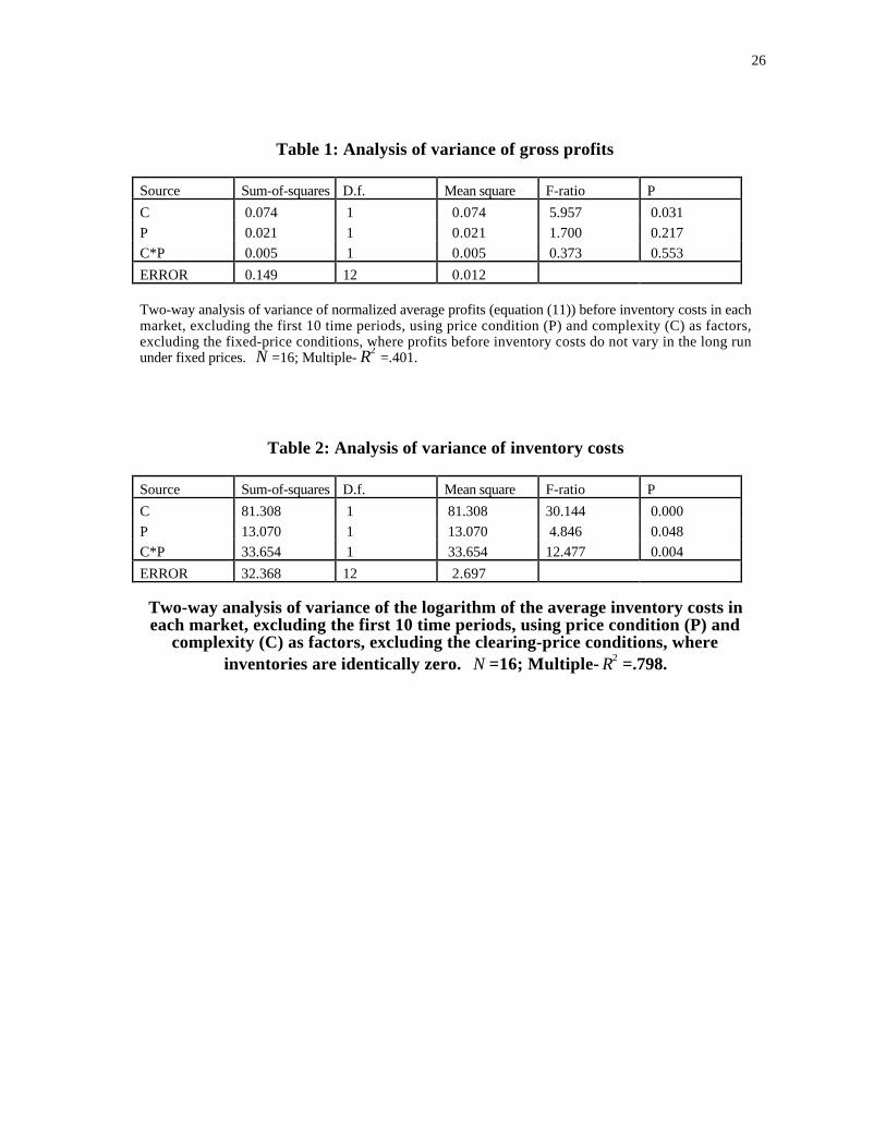
Table 1 reports analysis of variance of the normalized gross profits in the four price-varying conditions. While the price regime has no significant effect, the effect ofcomplexity is significant: On average, gross profits relative to optimal in the complexconditions are 10-15% lower than in the corresponding simple conditions, in some caseseven falling below the competitive equilibrium level.

Table 2 repeats the analysis for inventory costs alone, excluding the price-clearingcondition where inventories are zero. (Costs were transformed with logarithms tominimize differences in within-cell variance.) The hypothesis of constant inventory costsin the non-clearing conditions is strongly rejected (p<0.1%). Complexity has a very largeeffect on inventory costs – on average, inventory costs are about 13 times larger in thecomplex conditions. But there is also a strong interaction: the effect of complexity oninventory costs is much smaller in the posted-price than in the fixed-price regime.

Thus, the data show effects that do not follow from the standard assumptions of non-cooperation and rationality. In fact, these effects agree with the predictions of thebehavioral hypotheses: Profits relative to optimal are lowered by the introduction ofcomplexity in all three price regimes, sometimes dramatically. Most of the drop stemsfrom higher inventory costs (except of course in the price-clearing conditions), but profitsbefore inventory costs are lower as well. As a result, the effect of complexity on net profitis very large in the fixed-price and posted-price regimes, and smaller in the clearing-priceregime. Finally, there is much greater variance in profits in the complex posted and fixed-price cases than in the other four conditions (The Bartlett test for homogeneity of groupvariances in net profits shows significant differences at p<0.1%).

3.3. Effects on Market Dynamics and Convergence

Figure 2 showed examples of market adjustment when firms are "rational" in thefollowing sense: They correctly estimate the structural parameters of the system fromdata accumulated during the initial learning period; they are predetermined to eithercooperate or, in the case of Figure 2, to compete, and have correct expectations of thebehavior of other firms; and they act to maximize their expected profits, except for arandom uncorrelated error of 5% (see Kampmann 1992). In all six conditions, themarkets to a stochastic stationary state after less than 10 time periods. The variation inmarket averages differs across conditions, but in all cases it is lower than the variance ofany random errors in decision-making.

Figures 4-9 show the actual behavior of production and prices for each market for each ofthe experimental conditions. A quick glance reveals significant differences in the patternof behavior across the conditions. The complex markets generally show larger andlonger term variation in prices and quantities, and less tendency to converge toequilibrium, than the corresponding simple markets. There appear to be persistent

10

cyclical movements in several of the complex markets.

In the simple condition with fixed prices (Figure 4) production settles quickly in the ex-pected range. Apart from a few occasional departures from the equilibrium level,production is constant at its steady-state value. The task facing the decision maker here isa simple inventory control problem with a constant exogenous outflow. Indeed, the fixedprice simple condition is equivalent to running the tap in a bathtub with a constant outflowof water until the water level reaches a given target level. Previous experiments haveshown, unsurprisingly, that humans perform quite well under such simple circumstances(Diehl and Sterman 1995, MacKinnon and Wearing 1985).

The variation in production is dramatically larger in the fixed-price complex condition(Figure 5). All markets show substantial cycles of "boom and bust". The initial increasein demand leads to inventory depletion before additional output can go through thesupply line. In the face of rising demand and falling inventories, firms raise theirproduction, leading to still higher demand, which in turn causes firms to raise productionfurther. Because of the production delay and the continuous accumulation of inventoryimbalances, firms have great difficulty catching up with demand. The upward spiralcontinues until higher production restores normal inventory levels, at which point all firmscut their production, leading to a decrease in demand and excessive unintended inventoryaccumulation. The result is a "recession" where production falls below equilibrium. Thecycle in some markets is exceedingly large; in Market 25, output peaks at around fourtimes the equilibrium value. None of the markets show any sign of being in equilibriumat the end of the trial. The fixed-price complex condition is analogous to the setting inSterman’s (1989a) multiplier-accelerator experiment, and the results are quite similar.

The markets with clearing prices also show marked differences between the simple andthe complex condition. The markets in the simple clearing-price condition show nosystematic pattern of behavior (Figure 6). Some appear to settle in a range close to, orslightly above, the competitive price equilibrium, but with a fair amount of short-termfluctuation. Others show some longer-term fluctuation.

In contrast, the complex clearing-price markets all display a distinct "boom and bust"pattern of an initial dramatic overshoot in production, followed by a gradual downwardadjustment in output (Figure 7). Although the initial boom and bust is substantial, thecycle is not sustained as it is in the corresponding fixed-price condition.

A key structural difference between the fixed and clearing price regimes is the lack ofcumulative effects of market imbalances in the latter. In the fixed price conditions, anyinventory imbalances persist until corrected by subsequent production adjustmentsinitiated by the subjects. In the clearing price condition, the computer acts as a perfectWalrasian auctioneer, finding the market clearing prices that eliminate all inventoryimbalances each and every period. The relatively high firm- and industry- level demandelasticities mean that inventory imbalances caused by subjects’ decision errors arecorrected at low cost through modest price adjustments. Consequently, the market alwaysbegins the next round in balance, making it forgiving of past errors.

11

The posted-price markets also show effects of complexity on behavior. In the simplecondition (Figure 8), prices are relatively steady, and in three of the four markets, pricesseem to be driven down toward the competitive level. In market #32, firms change theirprices little throughout most of the game. In all markets, inventories are kept closely incheck and never depart substantially from the desired level, as they can be controlleddirectly through adjustments in production.

The posted-price complex condition generally shows larger variance in prices andproduction compared to the simple case, although the variance differs from market tomarket (Figure 9). Market #16 exhibits dramatic, expanding oscillations in prices andoutput. In markets #18 and #38 both prices and inventories, and in #18 also production,exhibit a cycle of rather steady amplitude and frequency. Market #17 shows relativelylittle variance in output or prices, except for a one-time peak in prices.

Spectral analysis confirmed what is evident from inspection of the results (seeKampmann 1992). While the spectra produced by rational agents will, after an initiallearning period, be either nearly white or concentrated in the high-frequency range, thespectra of the experimental markets in the all complex conditions show the variance isconcentrated in the low frequencies corresponding to the 10-20 period cycles or longerterm movements evident in the figures.

4. Individual heuristics and aggregate outcomes

The aggregate market outcomes show behavior is consistent with boundedly rationaldecision making, and in particular, the "misperceptions of feedback" hypothesis thatsubjects fail to account for time delays, accumulations and action feedback processes inthe decision environment. This section probes further into this idea by proposing simpledecision rules which capture much of the individual decisions made by subjects in theexperiments and, when embedded in a simulation of the complete market, reproduce thesalient features of the aggregate behavior. The analysis reported below focuses on twoconditions, the complex fixed-price and posted-price condition, respectively, since thecomplex conditions show the largest departures from rationality (the fixed price complexcondition is effectively equivalent to situations analyzed in prior work, e.g. Sterman1989a, b and Diehl and Sterman 1995). In the last section, an examination of the verbaland timing data collected during the experiments show that feedback complexity affectsthe degree to which firms manage to collude and indicate that firms' decisions becomemore reactive and simplistic as task complexity increases. Moreover, there is clearevidence that subjects attribute cyclical fluctuations in the market to exogenous factors,even though these dynamics were generated endogenously by their own actions.

Fixed prices, complex condition

In the fixed-price conditions, subjects make only one decision each period, namely howmuch production to initiate. In addition to this decision, subjects were asked to provide aforecast of future average demand. This forecast provides insight into subjects'expectations, a key component in production planning.

12

The output decision is an example of what Sterman has called generic stock managementtasks (1989a, b). Any reasonable decision rule, including the optimal rule, consists ofthree components. First, forecast expected demand xt

e for the time period when initiatedproduction will be finished.2 Second, look at current inventory nt and compare it to itsdesired level nd , which is zero here; adjust production upward if there is a deficit,downward if there is excess inventory. Third, look at the current supply line st ofinitiated but not yet finished production and compare this to the desired level s d ; adjustproduction upward if there is too little, downward if there is too much. This lattermechanism prevents cumulative over- or under-ordering because it recognizes the delaybetween ordering and finishing production. A simple equation, which also respects thenon-negativity constraint on production, specifies the output decision as

(12) yt = max 0, xte − nnt + s sd − st( ){ } ,

where n , s , and s d are constant parameters.

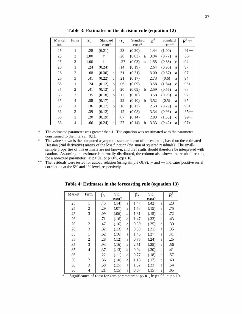
Table 3 shows the results of estimating equation (12), using the solicited forecasts for theexpectation xt

e and using nonlinear least-squares estimation.3 It is evident from the tablethat the fit is rather good; the R2 varies between .86 and .99.4 The table shows that mostsubjects pay some attention to their inventory levels: The coefficient is positive andsignificant in all but two cases, though it is generally less than one, indicating someconservatism in inventory adjustment. In contrast, attention to supply lines is much loweror absent: The coefficient is only significantly positive in four cases. Moreover, it issmaller than the inventory coefficient in all cases.

These results are in full accord with Sterman's findings (1989a, b). The low attentionpaid to the supply line is a key indicator of misperceptions of feedback: the subjects failto take sufficient account of the delay between initiating control actions and their impact.A simple metaphor would be a person with a headache who continues to take aspirinsuntil it goes away, instead of taking two pills and waiting for the effect. Such behavior israther more common than most people expect. For example, Alan Blinder (1997, 9-10),reflecting on his experience as Vice Chairman of the US Federal Reserve, describes withrefreshing candor how easy it is to underestimate delays:

...human beings have a hard time doing what homo economicus does so easily: waitingpatiently for the lagged effects of past actions to be felt. I have often illustrated this problemwith the parable of the thermostat. The following has probably happened to each of you; it has

2 In the following, the firm subscript i has been dropped for notational convenience.3 Equation (4.1) is in fact a Tobit model, for which consistent and asymptotically efficient

maximum-likelihood methods exist (Amemiya 1973). However, the small-sample properties ofthis method are not well-known. Simulations performed by Kampmann (1992) suggest that thenonlinear least-squares method gives better estimates in the case at hand.

4 The chosen R2 measures variations from zero and thus differs from the conventional measure of

variations around the sample mean. Our measure takes credit for predicting the absolute level aswell as variations around the mean, resulting in higher values.

13

certainly happened to me. You check in to a hotel where you are unfamiliar with the roomthermostat. The room is much too hot, so you turn down the thermostat and take a shower.Emerging 15 minutes later, you find the room still too hot. So you turn the thermostat downanother notch, remove the wool blanker, and go to sleep. At about 3 a.m., you awake shiveringin a room that is freezing cold.

The corresponding error in monetary policy leads to a strategy that I call ‘looking out thewindow.’ At each decision point, the central bank takes the economy’s temperature and, if it isstill too how (or too cold), proceeds to tighten (or to ease) monetary policy another notch. Withlong lags, you can easily see how such myopic decision making can lead a central bank tooverstay its policy stance, that is, to continue tightening or easing for too long.

...I cannot tell you how many times, both at the Federal Reserve and at meetings withforeign central bankers, discussions of future policy were cut short with phrases like ‘let’s seewhat happens’ or ‘we’ll have to wait until next month (or next meeting).’

A fully endogenous simulation of the market also requires modeling expectations. Thesolicited forecasts xt

e were fitted to a simple adaptive-extrapolative equation using pastvalues of the forecasted variable xt . Specifically,

(13) xte = xt −1

e + 1 xt − xt −1e( ) + 2 xt −1 − x t −2( ) .

The term with parameter 1 is an exponential moving average while the term withparameter 2 adds an extrapolation of recent movements in xt . Table 4 shows the resultsof estimating equation (13). The measure of fit varies between a low of 0.05 and a highof 0.75, with an average of 0.44.5 The adaptive parameter 1 is significant and notgreater than unity for all subjects. This indicates some conservatism in judgment, wheresubjects only adjust their forecasts gradually toward recent history. The extrapolativeparameter 2 is significant and positive in all cases. In fact, in over half the cases, it isgreater than unity, indicating a belief that changes in demand will accelerate.

Extrapolative expectations are highly dysfunctional in the experimental economy becausethey amplify the self-reinforcing feedback created by the aggregate demand multiplier: If,for instance, inventories are below their desired level, firms raise output to replenish them;the increase in output adds to aggregate demand through the multiplier; if firmsextrapolate this increase, they will want to increase output still more to accommodatefuture higher demand, thus increasing demand still further, in a positive feedback familiarto students of speculative bubbles from the tulip mania to the Japanese real estate marketof the 1980s. (This process is seen most clearly in market #25 in Figure 5, which alsohas the highest extrapolative coefficients in Table 4.)

Figure 10 shows the results of a fully endogenous simulation of each market in the fixedprice complex condition, where forecasts and output decisions are simulated with theestimated behavioral rules in equations (12) and (13) for each agent. The figure presentsboth the deterministic case with the estimated rules used alone, and an ensemble ofstochastic simulations where a random error is added to each decision. The errors are

5 The dependent variable in the regression is xt

e − xt −1e

, and the R2 is based on variations of this

variable from zero. Hence, this measure does not take credit for predicting the absolute value ofthe forecast.

14

assumed to be normal and i.i.d., with a standard deviation equal to the standard-error-of-estimate in the regressions.

Inspection of Figure 10 reveals that the simulations recreate both the relative variability ofthe four markets and the periodicity of the fluctuations. The deterministic simulationsshow greater stability than the corresponding observations and stochastic simulations--aclear example of the "bootstrap effect" (Dawes 1979), where the "human factor" in factreduces to random variance in the decision which decreases performance. When thisnoise is added in the stochastic simulations, the envelope of outcomes is very similar tothe observed history, though simulated performance is still slightly better than that of theactual subjects.

Kampmann (1992) supplements the visual inspection with more formal comparisons ofmarket performance and variability, all showing strong correlations between simulatedand actual results, with correlation coefficients of .95 or greater in all cases. In addition,he finds strong correlations between performance and certain coefficients in the decisionrules. In particular, profits are strongly correlated with the degree of attention to supplylines (the coefficient s in (12)), providing further evidence that the observed problematicbehavior result from misperceptions of feedback.

Posted-price, complex condition

In the posted-price condition, firms decide both on the amount of output to initiate and theprice to charge for their product each period. Moreover, subjects were asked to provideforecasts for future average sales and prices. Unlike the fixed-price condition, it is nowpossible for firms to manipulate the amount they sell by changing their price. Prices thusprovide a way to bypass a long production lag in regulating inventories. Indeed, theoptimal policy is to maintain production at the long-term profit-maximizing level, ignoringinventory costs and imbalances and instead use prices to control inventories (Kampmann1992, Appendix A).

The inventory-control component in price, combined with the long lags from initiation tocompletion of production makes it much more difficult for firms to signal collusion orpunish defections. Variability in prices is costly, due to the resulting inventoryfluctuations. Moreover, the presence of the multiplier effect makes it more difficult forfirms to discern whether they are operating in the right price-output range: Sales, andthus profits, are affected by the current amount of production in the pipeline, which mayvary substantially over time. Given these task characteristics, one would expect subjectsto devote less attention to strategic interaction and more attention to controllinginventories and judging trends. Output would be adjusted gradually to reflect long-termsales levels. Indeed, these notions were reflected in questionnaire responses (see below).

These considerations led to the following output decision rule, as a function of lastperiod's sales xt −1 and current inventory nt ,

(14) yt = yt −1 + 1 xt −1 − yt −1( ) + 2nt .

15

(There was no evidence that the supply line control entered decisions: In regressions witha supply line term included, all coefficients for this term were insignificant.)

The price decision was modeled by the equation

(15) pt = 0 + 1 Pte − 0( ) + 2nt ,

where Pte is the subject's observed price forecast. The rule represents the assumption that

subjects anchor their price on a weighted average of a long-term target price level, theparameter 0 , and their expectations of the aggregate price level Pt

e . They then modifythis anchor with the last term in (15) to adjust their inventory level toward zero (i.e., theparameter 2 should be negative).

Tables 5 and 6 report the results of the regressions. The pricing equation fares betterthan the output equation--the average R2 in Table 6 is .66, which is quite high for aregression with a constant term, and it is above .5 in all but two cases. The inventorycoefficient 2 is negative and significant in all cases except one. The coefficient 1 issignificant and close to unity in all but two cases, indicating that a large number ofsubjects are pure "followers" in that they anchor exclusively on the expected marketaverage price.

The production equation has less explanatory power (the average R2 is only .26). Thecoefficient is often significant and always between 0 and 1, indicating that subjects adjusttheir output gradually to past sales. The inventory coefficient is only significant in threecases, one of which with the wrong sign. Thus, it appears that subjects rarely useproduction to regulate inventories.

In modeling expectations, the simple adaptive-extrapolative rule was used as in the fixed-price case. Table 7 shows the results of estimating the forecasting rules (13) for averagesales and

(16) Pte = Pt−1

e + 1 Pt −1 − Pt −1e( ) + 2 Pt −1 + Pt −2( )

for average price, respectively. Generally, the rules explain the forecasts quite well (thelowest R2 is .07, the highest .81, and the average .45). Moreover the adaptive parameteris significant in all but two cases and always less than unity, for both demand and priceforecasts. There is some tendency to extrapolate trends--13 out of the 30 coefficientswere significant (and positive), though it less pronounced than in the fixed-price caseabove.

Figure 11 shows the result of incorporating the estimated decision- and forecasting rulesinto a complete endogenous simulation of each market, similar to the fixed-price caseabove.6 Comparing the simulated and observed prices in the figure, it is evident that the

6 The first three time periods incorporate actual decisions. Since the first three periods were part of

the practice round, one would expect there to be a fair amount of random experimentation.

16

proposed simple decision rules capture a great deal of the pattern of behavior in eachmarket: The relative variability as well as the period of fluctuation is the same. As in thefixed-price condition above, there is also a strong boot-strapping effect, resulting inhigher stability of the deterministic simulations. When random noise is added in thestochastic simulations, the cyclical tendencies of the observed outcomes reappear. That is,the estimated decision rules interact with the institutional environment and with oneanother to form a system whose frequency response attenuates very high frequencies butamplifies low frequencies to produce significant closed loop gain over a relatively widefrequency range. Therefore small random shocks are amplified into coherent lowfrequency oscillations.

The simulations also demonstrate how the observed tendency for some markets to cyclecan arise from the interaction of prices and inventories. If firms respond to inventoryimbalances by adjusting their prices downward and if they also anchor their decisions onlast period's average price, then prices will continue to drift lower as long as there is anexcess inventory. Eventually, the lower prices increase sales enough that inventories fallback toward their desired level, but by the time equilibrium has been reached, averageprice may now be close to its minimum, due to the cumulative drift, and sales may besubstantially above production. The results would be that inventories continue to fallbelow their desired level. If production also responds to inventory imbalances and iffirms do not account sufficiently for the supply line, the cycle is further amplified.

5. Effects of complexity on decision making

In addition to the actual decisions made by subjects, we instrumented the experiments tocollect a wealth of other data, including a complete record of all keystrokes and otherevents, providing a record of the time taken to deliberate decisions, post-trialquestionnaires asking about causes of the observed outcomes, and, for some subjects,concurrent verbal protocols of their entire session. These data yield additional insightsinto the way subjects approached the task and the accompanying "mental images" withwhich they represented this task, as well as the cognitive effort applied. Some of theseresults reflect appropriate adjustments of subject behavior to the task at hand, similar tothe results obtained by, e.g., Payne, et al. (1993). Others, however, point to inherentlimitations in subjects' understanding of the dynamic structure of the market, and thusgive evidence of bounded rationality and the impact of misperceptions of feedback.

Exogenous vs. endogenous accounts of dynamics

A key prerequisite for understanding and thus improving the performance of any systemis to attribute the correct causes to the behavior one observes. An important element ofmisperceptions of feedback that hampers this understanding is the human tendency tooverlook over look aspects of the problem generated internally by our own and our

Moreover, the initial decisions provide a shock to the system, moving it out of equilibrium sothat the subsequent adjustment process is more clearly revealed than if one incorporated adaptiverules from the beginning of the simulation.

17

competitors interaction with the system, in favor of "blaming the environment" or"exogenous factors". The tendency to focus on external environmental or dispositionalattributes of a situation rather than systemic explanations is closely related to the so-called‘fundamental attribution error’ documented in social psychology (Ross 1977; see e.g.Repenning and Sterman 1998 for an application to dynamic decision making inorganizations).

To gain a measure of this tendency, subjects were asked to sketch a time graph of theirbest guess of external factors that might have influenced overall demand in the market.While these sketches showed no distinct pattern in the simple conditions, the vastmajority of subjects in the complex conditions drew graphs that looked very similar to therealized aggregate sales rate in their market, even though there were in fact no exogenousinfluences on demand. For instance, in the fixed-price complex condition, 13 out of 14subjects drew an oscillatory pattern, even though it was pointed out to them that theremight not be any exogenous influences at all. Moreover, 12 out of the 14 emphasizedforecasting "the business cycle" or "trends" or "shifts" in demand, as seen in thefollowing quotes from the post-game questionnaire responses:

"Once I had the general pattern of a complete business cycle, I was able to make estimates of theaverage increase or decrease per period. ... It became clear after a while that given the instabilityof sales and the constant prices, profit maximization became simply inventory minimization."

"The major problem was determining the timing of the peaks and troughs of the business cycle,and my guess is that it's mostly due to external factors and thus hard to pinpoint exactly."

Only 2 out of the 14 subjects ever mentioned the multiplier effect – a key ingredient in thesystem's tendency to oscillate. These results are similar to the exogenous accounts of thecycle found in the "beer distribution game" (Sterman, 1989b).

If one believes that good performance primarily requires pinpointing a business cycle, orpredicting trends in demand, not realizing that cycles or trends may be self-generated,there is little possibility of learning from history. In fact, if a majority of agentsextrapolate current trends, the results can be devastating, as observed in Market #16 inFigure 9.

Decision timing and mental effort

A number of scholars in behavioral decision theory have posed the hypothesis that, givena certain psychological resistance to exerting cognitive effort, decision makers are likelyto adapt their heuristics for the task at hand, trading off the mental effort involved with theexpected quality of the decision (e.g., Payne, et al. 1993). More generally, a limitedcapacity to process information requires the individual to adopt simplified rules orheuristics (Simon, 1979).

One rough measure of mental effort is the amount of time spent in deliberation for eachdecision. As mentioned previously, the experimental protocol did not involve overt timepressure but still gave incentives to act quickly. Subjects were free to take as much timeas they wanted to make their decisions, although it was pointed out to them that taking

18

longer could result in fewer rounds played and, hence, in lower cumulative profits.

Since both the information processing requirements and the "leniency" of the task, i.e.,the "forgiveness" of the system to errors, differs across the experimental conditions, onewould expect deliberation times to vary as well. A more lenient system would allow forfaster decision making, while a more complex task would require more effort.

First, the mental effort required varies because the number of decisions was not the same:The fixed-price conditions involved one decision (output) and one forecast (sales); theclearing-price conditions also involved only one decisions but two forecasts (sales andprice); and the posted-price conditions involved both price and output decisions and botha price and demand forecast.

Second, the "arithmetic" of inventory control may be simpler than the task of finding theoptimal price-output pair. The inventory control task involves three steps: Form anexpectation of future demand and anchor production on this figure. Then, look at currentinventory and adjust production to account for a current excess or insufficient inventory.Finally, (in the complex condition only) look at the pipeline of unfinished production andadjust production if there is "too much" or "too little" in the pipeline. All these stepsinvolve addition or at least simple linear operations. In contrast, the task of finding theoptimal price-output position involves calculating marginal profits as a function of price,relative to market average price. None of these figures are readily available in theinformation display but must be calculated from tables or graphs.7 The posted-pricecondition is the most difficult because it involves both inventory control and price-outputoptimization.

Third, both the clearing-price and the posted-price regimes allow for possible collusionamong firms. Here, firms must also consider whether to cooperate or defect and how toget other firms to cooperate. All of these three task characteristics speak for the followingranking of deliberation times in both the simple and complex conditions: Fixed <clearing < posted.

On the other hand, the leniency of the tasks does not follow the same ordering. In theclearing-price regime, profits are not very sensitive to deviations in the output decisionsaround the optimal price-output point. In the two other regimes, the cost of excess orinsufficient inventory makes it more important to set production at the right level. Thus,even though the clearing-price regime involves one more forecast to make than the fixed-price regime, the overall deliberation time may be smaller, all other things equal, since theoutput decision is less crucial for performance. This would, all other things equal, call forthe following ranking of deliberation times: Clearing < fixed < posted.

7 Of course, one might imagine that subjects use a search procedure rather than trying to calculate

marginal profits. However, such a search is difficult because profits depend not only on thedecision parameter (price or output) but on other variables as well (other prices, the multipliereffect, etc.).

19

Finally, one would expect there to be a strong effect of complexity on decision times. Inall three price regimes, the introduction of complexity makes the task more difficult,though the added difficulty varies in the three price regimes. One would therefore expectthere to be some interaction effects on deliberation time between price regime andcomplexity.

In the fixed-price regimes, the difference between the simple and complex condition isprobably the largest. The simple fixed-price condition amounts to only a trivial inventorycontrol task in the face of constant demand. In the corresponding complex condition, thetask is complicated by the time lag and the supply line correction, and by the possiblelarge variations in demand caused by the multiplier effect.

In the clearing-price regime, the introduction of complexity is somewhat less important,since inventory accumulations are absent in this condition. Thus, by the time the startedproduction is ready to sell, the system will have "forgotten" all its history. In contrast,inventory accumulations in the other two price regimes perpetuate past errors in the formof inventory imbalances. The main complicating effect of complexity here is that themultiplier effect on demand influences the price level in the complex condition whereasthe average price in the simple condition only depends on average output. However, sinceprofits are not particularly sensitive to deviations from the optimal output choice, the agentcan get by quite well as long as the forecasted average price and output are not too far off.Thus, one would expect the clearing-price regime to show a smaller effect of complexityon deliberation time than the two other regimes.

The posted-price regime involves both the inventory-control element of the fixed-priceregime and the price-output search and strategic considerations of the clearing-priceregimes. Since each of these elements is compounded by the complexity treatment, onemight expect the effect of complexity on deliberation time to be largest in the posted-priceregime. On the other hand the treatment effects are unlikely to be additive in this fashion.The simple posted-price condition is "at least an order of magnitude" more complicatedthan the simple fixed-price condition since it involves both strategic behavior aspects, avariable demand, and a search for the best output-price position. Thus, whether the effectof complexity is larger in the fixed-price or the posted-price regime is ambiguous.

To summarize, the expected differences in deliberation times are based on the assumptionthat subjects on average will use more mental effort (measured by deliberation time) in themore difficult tasks (from an information-processing point of view), but that the effectwill also depend on the leniency of the system, i.e. how important it is to be close tooptimal. These considerations above leads to the following hypotheses about averagedeliberation times in the six experimental conditions:

20

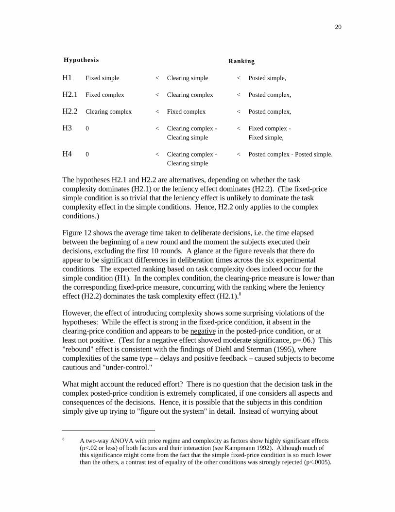
Hypothesis Ranking

H1 Fixed simple < Clearing simple < Posted simple,

H2.1 Fixed complex < Clearing complex < Posted complex,

H2.2 Clearing complex < Fixed complex < Posted complex,

H3 0 < Clearing complex -

Clearing simple

< Fixed complex -

Fixed simple,

H4 0 < Clearing complex -

Clearing simple

< Posted complex - Posted simple.

The hypotheses H2.1 and H2.2 are alternatives, depending on whether the taskcomplexity dominates (H2.1) or the leniency effect dominates (H2.2). (The fixed-pricesimple condition is so trivial that the leniency effect is unlikely to dominate the taskcomplexity effect in the simple conditions. Hence, H2.2 only applies to the complexconditions.)

Figure 12 shows the average time taken to deliberate decisions, i.e. the time elapsedbetween the beginning of a new round and the moment the subjects executed theirdecisions, excluding the first 10 rounds. A glance at the figure reveals that there doappear to be significant differences in deliberation times across the six experimentalconditions. The expected ranking based on task complexity does indeed occur for thesimple condition (H1). In the complex condition, the clearing-price measure is lower thanthe corresponding fixed-price measure, concurring with the ranking where the leniencyeffect (H2.2) dominates the task complexity effect (H2.1).8

However, the effect of introducing complexity shows some surprising violations of thehypotheses: While the effect is strong in the fixed-price condition, it absent in theclearing-price condition and appears to be negative in the posted-price condition, or atleast not positive. (Test for a negative effect showed moderate significance, p=.06.) This"rebound" effect is consistent with the findings of Diehl and Sterman (1995), wherecomplexities of the same type – delays and positive feedback – caused subjects to becomecautious and "under-control."

What might account the reduced effort? There is no question that the decision task in thecomplex posted-price condition is extremely complicated, if one considers all aspects andconsequences of the decisions. Hence, it is possible that the subjects in this conditionsimply give up trying to "figure out the system" in detail. Instead of worrying about

8 A two-way ANOVA with price regime and complexity as factors show highly significant effects

(p<.02 or less) of both factors and their interaction (see Kampmann 1992). Although much ofthis significance might come from the fact that the simple fixed-price condition is so much lowerthan the others, a contrast test of equality of the other conditions was strongly rejected (p<.0005).

21

optimizing, they may resort to "damage control." Subjects' pricing policy may revert to asimple heuristic along the following lines, ignoring any attempts at searching for the bestprice-output point or signaling collusion: 1) form expectation about average price, andanchor on this average, and 2) adjust the anchor up or down, depending on whetherinventory is negative or positive. Indeed, these considerations led to the heuristic rule(15) above.

There is also evidence from the post-game questionnaires that subjects concentrated moreon inventory control in their pricing policy in the complex posted-price condition and lesson strategic interaction with other firms. We coded subject questionnaire responses forterms indicating strategic or game theoretic reasoning, such as 'collusion', 'signal','cooperate', 'free rider', 'support prices', etc. Only 3 out of 15 subjects in the posted pricecomplex condition mentioned terms indicating strategic reasoning. In the correspondingsimple condition, 16 out of 20 subjects used such terms. The difference is highlysignificant.9 Conversely, the responses in the complex posted-price condition containedfrequent references to using prices to control inventory, as seen in the following quotes:

"The price decision generally attempted to clear out the planned production and inventory."

"I attempted to use my price-setting to manipulate what my sales in that period would be. If Iwanted to dampen demand, I overcharged, if I wanted to boost sales, I undercharged."

"I set price above or below market price depending on how I needed to manipulate my inventory... Price was my primary decision maker. Production stayed relatively constant."

"Optimal price seemed to be about 6.3, and demand could support 375 units at this price. I triedto hold things there, so I matched production to my anticipated sales. I occasionally used priceto throttle demand to stabilize inventory but more commonly, I regulated production based onanticipated sales and inventories."

"I played it safe--mostly keeping my prices close the average market price, except when I wastrying to unload inventory."

"I tried to make my prices follow the market to minimize my inventory. If I had positiveinventory, I had to sell at lower prices to get rid of them. "

9 out of the 15 subjects in this condition made such remarks while only 1 out of 20 didso in the simple posted-price condition--again a highly significant difference.10

It is interesting to note that rational agents should indeed use prices as an inventorycontrol measure in the complex posted-price condition but not in the correspondingsimple condition (see Kampmann 1992, Appendix A). However, deriving this resultanalytically is exceedingly difficult, and a more reasonable interpretation of the outcomehere is that subjects were forced into a reactive price-setting rule, as their inventoriesfluctuated.

9 The Fisher-Irwin exact test of equal proportions is rejected at p<.0005.10 The one-tailed Fisher-Irwin exact test rejects equal proportions at p=.001.

22

A slightly different explanation may be offered for the absence of any complexity effectin the clearing-price regime. The lack of any effect is certainly surprising, since bothcommunication and figuring out the best price-output level is much harder in the clearing-price regime. On the other hand, the fact that both the simple and the complex price-clearing conditions are quite forgiving of errors may induce subjects over time, as theydiscover this leniency, to worry less about making "the right" decisions and instead try tomake more decisions.

In conclusion, the results do not indicate that the observed mental effort uniformlyfollows the objective properties of the task; although there is evidence for some of theeffects one would expect based on this perspective, there does seem to be a threshold levelof complexity beyond which mental effort is reduced, or at least not increased. Instead,subjects appear to resort to simplified heuristics. In particular, subjects appear to give upworrying about strategic interaction when the dynamic structure becomes sufficientlycomplex.

6. Conclusions

The experimental results demonstrate that bounded rationality, and in particular,misperceptions of feedback, can have large effects on market behavior. The results alsoshow that the consequences of bounded rationality and dynamically deficient mentalmodels of the environment depend strongly on the pricing institution employed. Theeffects of bounded rationality are most dramatic in the fixed-price regime, where subjectsgenerated sustained cycles, replicating previous non-market studies despite financialincentives for performance. In the clearing-price regime, automatic market clearingsuppresses the accumulation of imbalances and thus makes the system much moreforgiving of poor attention to delays and feedback. In the posted-price regime, thepossibility of using prices to control inventories makes the system potentially easier tohandle. However, in three out of the four markets, inventories and prices continue tooscillate throughout the trial: the cycle involving output and inventories in the fixed-pricecondition is replaced by one involving prices and inventories in the posted-pricecondition. While much of the decrease in profits is the result of excessive inventoryfluctuations, the introduction of complexity also made it more difficult for firms to findthe price-output level that would maximize profits before inventory costs.

Thus, markets seem to moderate, but do not eliminate, the effects of decision-makers'misperceptions of feedback structure. The mere existence of markets does not imply thatindividual misperceptions of feedback are automatically ameliorated. Misperceptionscontinue to occur, but their consequences are a function of the dynamic structure of themarket setting. Therefore, models of economic dynamics must be grounded in empiricalstudy of managerial decision making to capture the bounded rationality and deficientmental models of the agents – the misperceptions of feedback – that may producesystematic and persistent deviations from rational behavior even in the presence of well-functioning market institutions.

The study highlights the importance of linking studies of individual decisions to theresulting aggregate outcomes. Individual choices interact with the surrounding system to

23

produce aggregate dynamics. The study shows decision rules characterizing individualdecisions can be estimated from experimental data. Furthermore, it was possible tointerpret the coefficients in the decision rules in terms of underlying psychologicaldecision heuristics such as anchoring and adjustment. The estimated rules can then betested in simulations of the entire system, creating an ecology of simulated interactingagents, each of which is endowed with decision rules grounded in study of actual humandecision making. The behavior of the simulated economy replicated many of the salientfeatures of the observed market outcomes, providing an explicit link from themicrostructure of decision making and the institutional environment to the macrobehaviorof the system.

The study also shows how a variety of data sources, such as verbal protocols and timingdata, can be used to gain insight into the mental processes involved at the individual level.In particular, we showed how decision makers cope with increasing complexity bynarrowing the scope of their decisions from broad considerations of strategic interactionsamong firms to a more reactive concern with inventory control. Since the data are easy tocollect, particularly when the experiment is computerized, we recommend that futurestudies in experimental economics make more use of such sources.

An important question that has only partially been addressed here is the scope forlearning in changing behavior over time. Indeed, a frequent criticism of experimentalstudies is that they employ inexperienced subjects and/or do not allow for sufficientlearning.

The psychological literature on learning has shown that effective learning is possible onlywhen there is immediate and unambiguous feedback from the environment. If feedbackis delayed or distorted, or if simultaneous side effects complicate the outcomes, learningability declines significantly (Brehmer 1980, Brehmer 1992). Thus, the potential forlearning must clearly be strongly affected by the feedback structure of the system, againemphasizing the need for explicit considerations of this element in economic theorybuilding.

Although we considered learning partly outside the scope of this work, the results castsome doubt on its potential. The questionnaire and protocol data show there is atendency for subjects to believe that observed fluctuations are caused by exogenousfactors rather than by their own interactions with the system. This false attribution couldbecome a strong impediment to learning. Indeed, Kampmann (1992) included ananalysis of learning, defined as a change in the parameter values of decision functions andan improvement of forecasting consistency and accuracy. Apart from the very first partof the game, there was little evidence of learning. (In the analysis presented here, the first10 periods were excluded to remove this initial learning effect.) Similar results arereported in Paich and Sterman (1993).

Nonetheless, it is fair to say that many issues relating to learning, particularly inqualitative changes in decision heuristics, remains to be explored. The same could be saidof competitive selection and endogenous market dominance by firms.

24

Another caveat relates to the external validity of the experiment. To what extent canlaboratory settings with relatively young participants tell us about real-world decisionmaking? This is a familiar issue in the debate between psychologists and economists (seee.g., Hogarth and Reder 1987) and will not be discussed in detail here, except to say thatother dynamic decision-making experiments have explored the effect of experience,education, and expertise on performance and have not found any significant differences(e.g., Bakken 1992).

One step toward assessing the real-world validity of the results would be to try to classifyindustries according to their feedback structure (production and product-developmentdelays, market institution, etc.) and relate their feedback properties to measures of marketstability. A systematic study of this issue remains to be done, but it has long been knownthat industries and firms with long gestation and construction delays and supply chainscontaining substantial resource accumulations such as inventories (e.g. real estate,semiconductors, automobiles, shipbuilding, commodities, machine tools) experience muchmore instability than industries and firms lacking these elements of dynamic complexity(such as consumer services).

References

Amemiya, T. (1973) "Regression Analysis when the Dependent Variable is TruncatedNormal" Econometrica 41: 997-1016.

Arrow, K.J. (1987). "Rationality of self and others in an economic system." In Hogarth,R.M. and Reder, M.W., ed. Rational choice: The contrast between psychology andeconomics. Chicago, IL: Univ. of Chicago Press.

Bakken, B. E. 1992 Learning and transfer in simulated dynamic environments, " PhD.Dissertation, MIT Sloan School of Management., Cambridge, MA.

Blinder, A. (1997) “What Central Bankers Could Learn from Academics – and ViceVersa,” Journal of Economic Perspectives 11(2), 3-19.

Brehmer, B. (1980) "In One Word: Not From Experience" Acta Psychologica 45: 233-241.

Brehmer, B. (1992) "Dynamic Decision Making: Human Control of Complex Systems"Acta Psychologica 81: 211-241.

Dawes, R. M. (1979) "The robust beauty of improper linear models in decision making"American Psychologist 34: 571-82.

Diehl, E., & Sterman, J. D. (1995). Effects of Feedback Complexity on DynamicDecision Making. Organizational Behavior and Human Decision Processes 62(2),198-215.

Fudenberg, D. and J. Tirole (1991) Game Theory Cambridge, MA: MIT Press.

Funke, J. (1991) "Solving Complex Problems: Exploration and Control of ComplexSystems" in Sternberg, R. and P. Frensch, ed. Complex Problem Solving: Principlesand Mechanisms Hillsdale, NJ: Lawrence Erlbaum Associates.

Hauthakker, H. S. and L. C. Taylor (1970) Consumer demand in the United StatesCambridge, MA: Harvard University Press.

25

Hogarth, R. M. and M. W. Reder (1987) Rational Choice: The Contrast betweenEconomics and Psychology Chicago: Univ. of Chicago Press.

Kampmann, C. (1992) "Feedback Complexity and Market Adjustment: An ExperimentalApproach" PhD. Dissertation, MIT Sloan School of Management., Cambridge, MA.

Kleinmuntz, D. (1985) "Cognitive Heuristics and feedback in a dynamic decisionenvironment" Management Science 31: 680-702.

MacKinnon, A. J. and A. J. Wearing (1985) "Systems Analysis and Dynamic DecisionMaking" Acta Psychologica 58: 159-72.

Paich, M., & Sterman, J. D. (1993). Boom, Bust, and Failures to Learn in ExperimentalMarkets. Management Science 39(12), 1439-1458.

Payne, J.W., Bettman, J.R. and Johnson, E.J. (1993). The Adaptive Decision MakerCambridge: Cambridge University Press.

Plott, C. R. (1982) "Industrial Organization Theory And Experimental Economics"Journal of Economic Literature 20: 1485-1527.

Plott, C. R. (1986) "Laboratory Experiments in Economics: The Implications of Posted-Price Institutions" Science 232: 732-38.

Repenning, N. P., & Sterman, J. D. (1998). Getting Quality the Old Fashioned Way:Self-Confirming Attributions in the Dynamics of Process Improvement. Workingpaper available from authors, MIT Sloan School of Management, Cambridge MA02142. Forthcoming in Scott, R. & Cole, R. (Eds.), The Quality Movement inAmerica: Lessons for Theory and Research

Ross, L. 1977. The intuitive psychologist and his shortcomings: Distortions in theattribution process. In L. Berkowitz (ed.), Advances in experimental socialpsychology, vol. 10. New York: Academic Press.

Sargent, T. (1993) Bounded Rationality in Macroeconomics. Oxford: Clarendon Press.

Simon, H.A. (1979). "Rational decision making in business organizations." AmericanEconomic Review. 69(4).

Smith, V.; G. Suchanek and A. Williams (1988) "Bubbles, Crashes, and EndogenousExpectations in Experimental Spot Asset Markets" Econometrica 56: 1119-1152.

Smith, V. L. (1982) "Microeconomic Systems as an Experimental Science" AmericanEconomic Review 72: 923-55.

Smith, V. L. (1986) "Experimental methods in the political economy of exchange"Science 234: 167-235.

Sterman, J. D. (1989a) "Misperceptions of Feedback in Dynamic Decision Making"Organizational Behavior and Human Decision Processes 43: 301-335.

Sterman, J. D. (1989b) "Modeling managerial behavior: Misperceptions of feedback in adynamic decisionmaking experiment" Management Science 35: 321-339.

26

Table 1: Analysis of variance of gross profits

Source Sum-of-squares D.f. Mean square F-ratio P

C 0.074 1 0.074 5.957 0.031

P 0.021 1 0.021 1.700 0.217

C*P 0.005 1 0.005 0.373 0.553

ERROR 0.149 12 0.012

Two-way analysis of variance of normalized average profits (equation (11)) before inventory costs in eachmarket, excluding the first 10 time periods, using price condition (P) and complexity (C) as factors,excluding the fixed-price conditions, where profits before inventory costs do not vary in the long rununder fixed prices. N =16; Multiple- R2

=.401.

Table 2: Analysis of variance of inventory costs

Source Sum-of-squares D.f. Mean square F-ratio P

C 81.308 1 81.308 30.144 0.000

P 13.070 1 13.070 4.846 0.048

C*P 33.654 1 33.654 12.477 0.004

ERROR 32.368 12 2.697

Two-way analysis of variance of the logarithm of the average inventory costs ineach market, excluding the first 10 time periods, using price condition (P) and

complexity (C) as factors, excluding the clearing-price conditions, whereinventories are identically zero. N =16; Multiple- R2 =.798.

27

Table 3: Estimates in the decision rule (equation 12)

† The estimated parameter was greater than 1. The equation was reestimated with the parameterconstrained to the interval [0,1].

* The value shown is the computed asymptotic standard error of the estimate, based on the estimatedHessian (2nd derivative) matrix of the loss function (the sum of squared residuals). The small-sample properties of this estimate are not known, and the results should therefore be interpreted withcaution. Assuming the estimate is normally distributed, the column also shows the result of testingfor a non-zero parameter: a: p<.01, b: p<.05, c:p<.10.

** The residuals were tested for autocorrelation (using simple OLS). + and ++ indicates positive serialcorrelation at the 5% and 1% level, respectively.

Table 4: Estimates in the forecasting rule (equation 13)

Marketno.

Firmn

Standarderror*

sStandarderror*

s d Standarderror*

R2**

25 1 .28 (0.21) .23 (0.20) 1.44 (1.00) .91++

25 2 1.00 † .20 (0.03) a 3.04 (0.77) a .86++

25 3 1.00 † -.27 (0.03) a 1.55 (0.88) c .94

26 1 .24 (0.24) .14 (0.19) 2.64 (0.96) a .97

26 2 .68 (0.36) c .31 (0.21) 3.00 (0.37) a .97

26 3 .41 (0.22) c .21 (0.17) 2.73 (0.6) a .94

35 1 .24 (0.12) b .06 (0.09) 3.58 (1.84) c .95+

35 2 .41 (0.12) a .20 (0.09) b 2.59 (0.56) a .88

35 3 .35 (0.18) b .12 (0.10) 3.58 (0.95) a .97++

35 4 .58 (0.17) a .22 (0.10) b 3.52 (0.5) a .95

36 1 .36 (0.17) b .16 (0.13) 2.53 (0.79) a .90+

36 2 .39 (0.12) a .12 (0.08) 3.34 (0.98) a .85++

36 3 .20 (0.19) .07 (0.14) 2.83 (1.55) c .99++

36 4 .66 (0.24) a .27 (0.14) b 3.33 (0.42) a .97+

Market Firm1

Std.error*

2Std.

error*R2

25 1 .45 (.14) a 1.47 (.42) a .2325 2 .29 (.07) a 1.58 (.15) a .7525 3 .09 (.06) a 1.31 (.15) a .7226 1 .71 (.16) a 1.47 (.33) a .4326 2 .47 (.16) a 0.50 (.25) a .3026 3 .32 (.13) a 0.59 (.21) a .3535 1 .62 (.16) a 1.45 (.27) a .4135 2 .28 (.12) a 0.75 (.24) a .2535 3 .93 (.16) a 2.51 (.35) a .5635 4 .37 (.13) a 0.94 (.20) a .4136 1 .22 (.11) a 0.77 (.18) a .5736 2 .36 (.10) a 1.15 (.17) a .6036 3 .58 (.15) a 1.52 (.23) a .5436 4 .21 (.15) a 0.07 (.15) a .05

* Significance of t-test for zero parameter: a: p<.01, b: p<.05, c: p<.10.

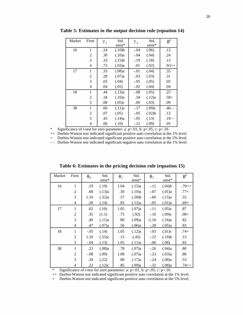
28

Table 5: Estimates in the output decision rule (equation 14)

Table 6: Estimates in the pricing decision rule (equation 15)

Market Firm1

Std.error*

2Std.

error*R2

16 1 .24 (.10)b -.04 (.06) .132 .30 (.10)a -.04 (.04) .243 .33 (.15)b -.19 (.18) .134 .73 (.03)a .01 (.02) .93++

17 1 .33 (.08)a -.01 (.04) .352 .28 (.07)a -.03 (.03) .313 .03 (.04) -.05 (.05) .054 .04 (.05) -.02 (.04) .04

18 1 .44 (.13)a -.08 (.05) .252 .34 (.10)a .34 (.12)a .58+3 .08 (.05)c .00 (.03) .09

38 1 .66 (.11)a -.17 (.09)c .46- -2 .07 (.05) -.05 (.02)b .123 .43 (.14)a -.05 (.13) .19- -4 .06 (.10) -.12 (.09) .05

* Significance of t-test for zero parameter: a: p<.01, b: p<.05, c: p<.10.++ Durbin-Watson test indicated significant positive auto correlation at the 1% level.+ Durbin-Watson test indicated significant positive auto correlation at the 5% level.- - Durbin-Watson test indicated significant negative auto correlation at the 1% level.

Market Firm0

Std.error*

1Std.

error*2

Std.error*

R2

16 1 .19 (.19) 1.04 (.15)a -.11 (.04)b .70++

2 .68 (.13)a .50 (.10)a -.07 (.01)a .77+

3 1.10 (.32)a .57 (.28)b -.60 (.15)a .55

4 .20 (.14) .83 (.12)a -.05 (.01)a .69+

17 1 .02 (.10) 1.05 (.07)a -.11 (.05)c .87

2 .35 (1.1) .75 (.92) -.16 (.09)c .08+

3 .49 (.11)a .80 (.09)a -1.16 (.16)a .82

4 .47 (.07)a .56 (.06)a -.28 (.05)a .83

18 1 -.05 (.14) 1.05 (.12)a -.03 (.01)c .74+

2 1.10 (.55)c .15 (.45) -.22 (.10)b .13

3 -.04 (.13) 1.05 (.11)a -.06 (.06) .83

38 1 .23 (.08)a .78 (.07)a -.26 (.04)a .80

2 -.08 (.09) 1.08 (.07)a -.23 (.03)a .88

3 .34 (.22) .80 (.17)a -.24 (.08)a .53

4 .22 (.12)c .85 (.09)a -.32 (.08)a .74++* Significance of t-test for zero parameter: a: p<.01, b: p<.05, c: p<.10.++ Durbin-Watson test indicated significant positive auto correlation at the 1% level.+ Durbin-Watson test indicated significant positive auto correlation at the 5% level.

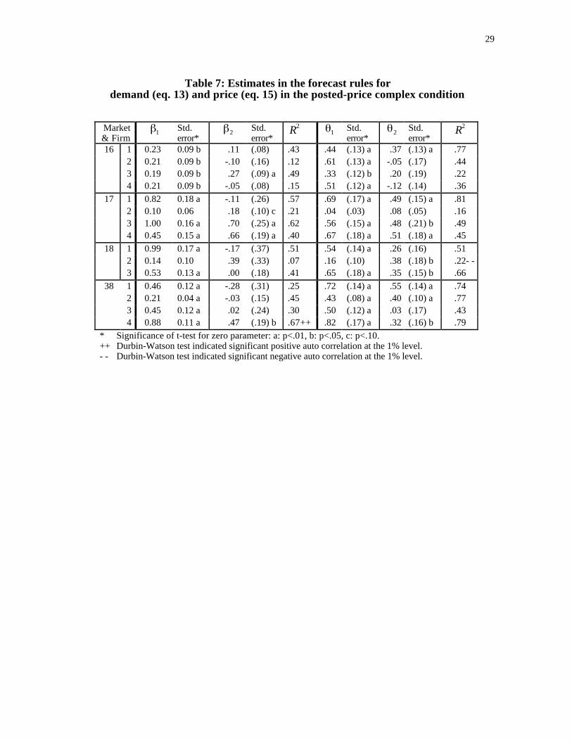
29

Table 7: Estimates in the forecast rules fordemand (eq. 13) and price (eq. 15) in the posted-price complex condition

Market& Firm

1Std.error*

2Std.error*

R21

Std.error*

2Std.error*

R2

16 1 0.23 0.09 b .11 (.08) .43 .44 (.13) a .37 (.13) a .772 0.21 0.09 b -.10 (.16) .12 .61 (.13) a -.05 (.17) .443 0.19 0.09 b .27 (.09) a .49 .33 (.12) b .20 (.19) .224 0.21 0.09 b -.05 (.08) .15 .51 (.12) a -.12 (.14) .36

17 1 0.82 0.18 a -.11 (.26) .57 .69 (.17) a .49 (.15) a .812 0.10 0.06 .18 (.10) c .21 .04 (.03) .08 (.05) .163 1.00 0.16 a .70 (.25) a .62 .56 (.15) a .48 (.21) b .494 0.45 0.15 a .66 (.19) a .40 .67 (.18) a .51 (.18) a .45

18 1 0.99 0.17 a -.17 (.37) .51 .54 (.14) a .26 (.16) .512 0.14 0.10 .39 (.33) .07 .16 (.10) .38 (.18) b .22- -3 0.53 0.13 a .00 (.18) .41 .65 (.18) a .35 (.15) b .66

38 1 0.46 0.12 a -.28 (.31) .25 .72 (.14) a .55 (.14) a .742 0.21 0.04 a -.03 (.15) .45 .43 (.08) a .40 (.10) a .773 0.45 0.12 a .02 (.24) .30 .50 (.12) a .03 (.17) .434 0.88 0.11 a .47 (.19) b .67++ .82 (.17) a .32 (.16) b .79

* Significance of t-test for zero parameter: a: p<.01, b: p<.05, c: p<.10.++ Durbin-Watson test indicated significant positive auto correlation at the 1% level.- - Durbin-Watson test indicated significant negative auto correlation at the 1% level.

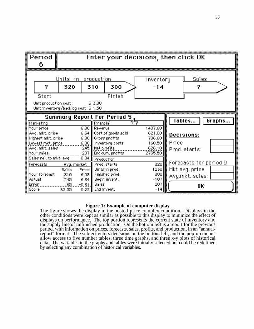
30

Figure 1: Example of computer displayThe figure shows the display in the posted-price complex condition. Displays in theother conditions were kept as similar as possible to this display to minimize the effect ofdisplays on performance. The top portion represents the current state of inventory andthe supply line of unfinished production. On the bottom left is a report for the previousperiod, with information on prices, forecasts, sales, profits, and production, in an "annual-report" format. The subject enters decisions on the bottom left, and the pop-up menusallow access to five number tables, three time graphs, and three x-y plots of historicaldata. The variables in the graphs and tables were initially selected but could be redefinedby selecting any combination of historical variables.

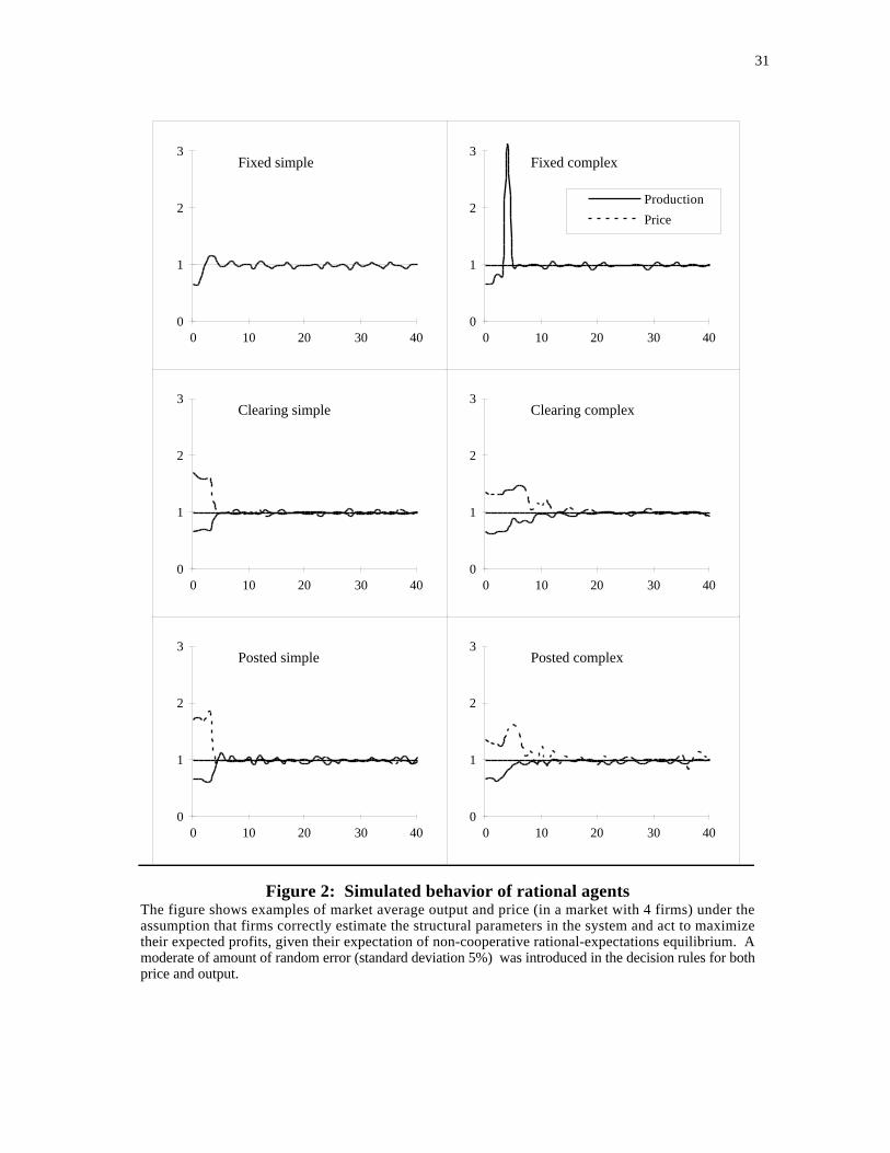
31

0

1

2

3

0 10 20 30 40

Posted complex

0

1

2

3

0 10 20 30 40

Clearing complex

0

1

2

3

0 10 20 30 40

Posted simple

0

1

2

3

0 10 20 30 40

Clearing simple

0

1

2

3

0 10 20 30 40

Fixed complex

0

1

2

3

0 10 20 30 40

Fixed simple

Production

Price

Figure 2: Simulated behavior of rational agentsThe figure shows examples of market average output and price (in a market with 4 firms) under theassumption that firms correctly estimate the structural parameters in the system and act to maximizetheir expected profits, given their expectation of non-cooperative rational-expectations equilibrium. Amoderate of amount of random error (standard deviation 5%) was introduced in the decision rules for bothprice and output.

32

-4

-3.5

-3

FixedSimple

FixedComplex

ClearingSimple

ClearingComplex

PostedSimple

PostedComplex

-1

-0.5

0

0.5

1

-1

-0.5

0

0.5

1

Gross Profits

Net Profits

Figure 3 Observed performance compared to simulated rational agentsThe figure shows gross and net average market profits (excluding the first 10 periods) observed in theexperiments (white bars), compared to simulations of rational non-cooperating agents (gray bars) whocorrectly estimate the structural parameters of the system, have rational expectations, and act inaccordance with maximization of expected profits, except for a random error (with standard deviation5%).. The diamonds indicate individual markets for the observed values and standard deviations for thesimulated values.

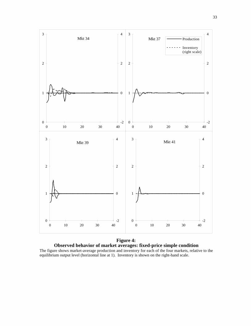
33

0

1

2

3

0 10 20 30 40-2

0

2

4Mkt 34

0

1

2

3

0 10 20 30 40-2

0

2

4Mkt 37

0

1

2

3

0 10 20 30 40-2

0

2

4Mkt 39

0

1

2

3

0 10 20 30 40-2

0

2

4Mkt 41

Production

Inventory(right scale)

Figure 4:Observed behavior of market averages: fixed-price simple condition

The figure shows market-average production and inventory for each of the four markets, relative to theequilibrium output level (horizontal line at 1). Inventory is shown on the right-hand scale.

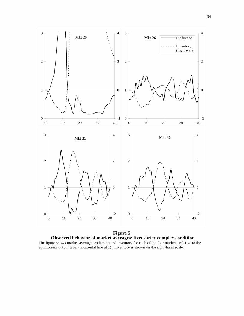
34

0

1

2

3

0 10 20 30 40-2

0

2

4Mkt 25

0

1

2

3

0 10 20 30 40-2

0

2

4Mkt 26

0

1

2

3

0 10 20 30 40-2

0

2

4Mkt 35

0

1

2

3

0 10 20 30 40-2

0

2

4Mkt 36

Production

Inventory(right scale)

Figure 5:Observed behavior of market averages: fixed-price complex condition

The figure shows market-average production and inventory for each of the four markets, relative to theequilibrium output level (horizontal line at 1). Inventory is shown on the right-hand scale.

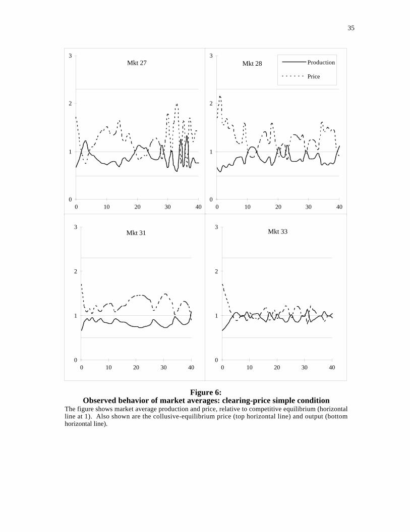
35

0

1

2

3

0 10 20 30 40

Mkt 27

0

1

2

3

0 10 20 30 40

Mkt 28

0

1

2

3

0 10 20 30 40

Mkt 31

0

1

2

3

0 10 20 30 40

Mkt 33

Production

Price

Figure 6:Observed behavior of market averages: clearing-price simple condition

The figure shows market average production and price, relative to competitive equilibrium (horizontalline at 1). Also shown are the collusive-equilibrium price (top horizontal line) and output (bottomhorizontal line).

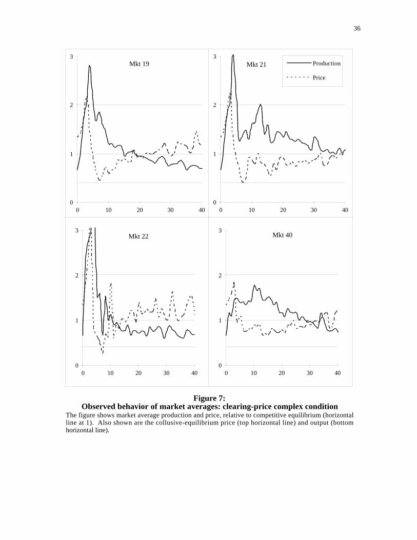
36

0

1

2

3

0 10 20 30 40

Mkt 19

0

1

2

3

0 10 20 30 40

Mkt 21

0

1

2

3

0 10 20 30 40

Mkt 22

0

1

2

3

0 10 20 30 40

Mkt 40

Production

Price

Figure 7:Observed behavior of market averages: clearing-price complex condition

The figure shows market average production and price, relative to competitive equilibrium (horizontalline at 1). Also shown are the collusive-equilibrium price (top horizontal line) and output (bottomhorizontal line).

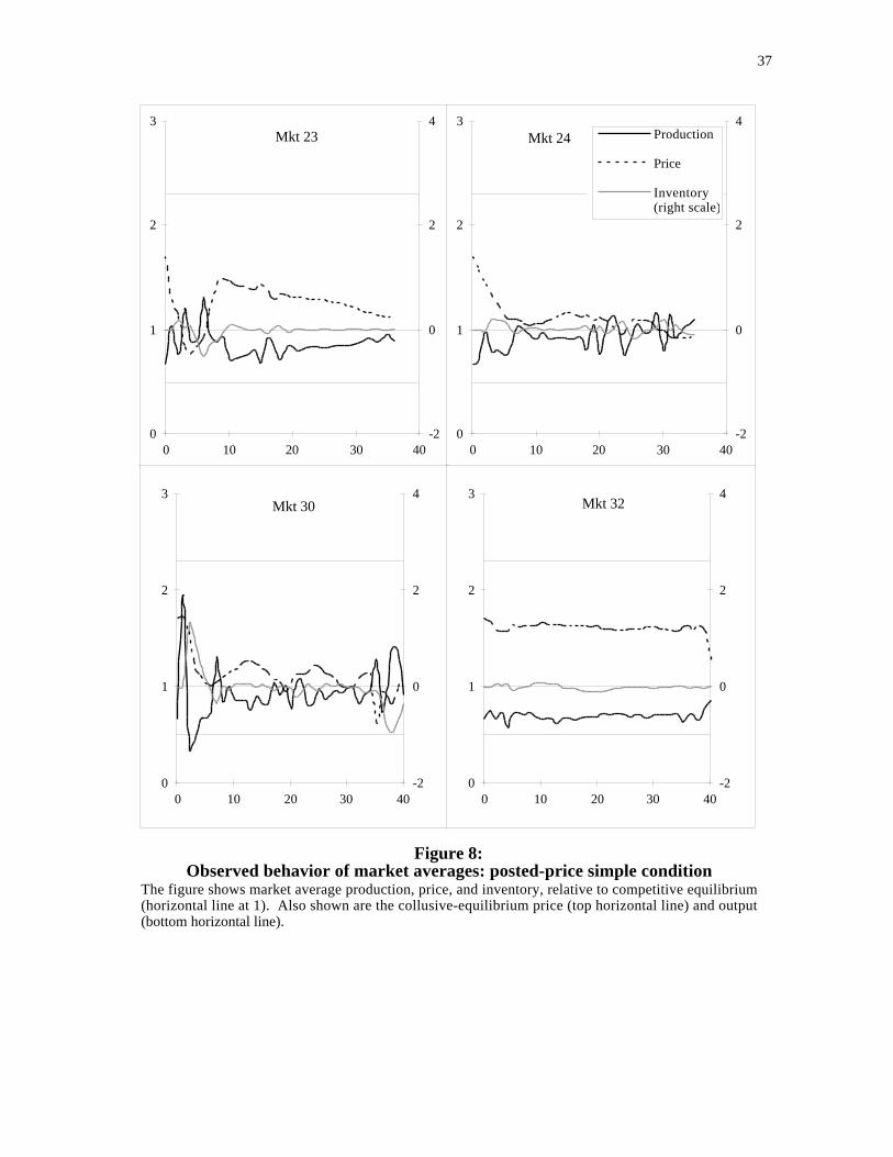
37

0

1

2

3

0 10 20 30 40-2

0

2

4Mkt 23

0

1

2

3

0 10 20 30 40-2

0

2

4Mkt 24

0

1

2

3

0 10 20 30 40-2

0

2

4Mkt 30

0

1

2

3

0 10 20 30 40-2

0

2

4Mkt 32

Production

Price

Inventory(right scale)

Figure 8:Observed behavior of market averages: posted-price simple condition

The figure shows market average production, price, and inventory, relative to competitive equilibrium(horizontal line at 1). Also shown are the collusive-equilibrium price (top horizontal line) and output(bottom horizontal line).

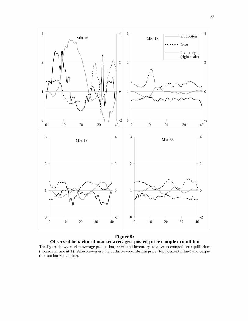
38

0

1

2

3

0 10 20 30 40-2

0

2

4Mkt 16

0

1

2

3

0 10 20 30 40-2

0

2

4Mkt 17

0

1

2

3

0 10 20 30 40-2

0

2

4Mkt 18

0

1

2

3

0 10 20 30 40-2

0

2

4Mkt 38

Production

Price

Inventory(right scale)

Figure 9:Observed behavior of market averages: posted-price complex condition

The figure shows market average production, price, and inventory, relative to competitive equilibrium(horizontal line at 1). Also shown are the collusive-equilibrium price (top horizontal line) and output(bottom horizontal line).

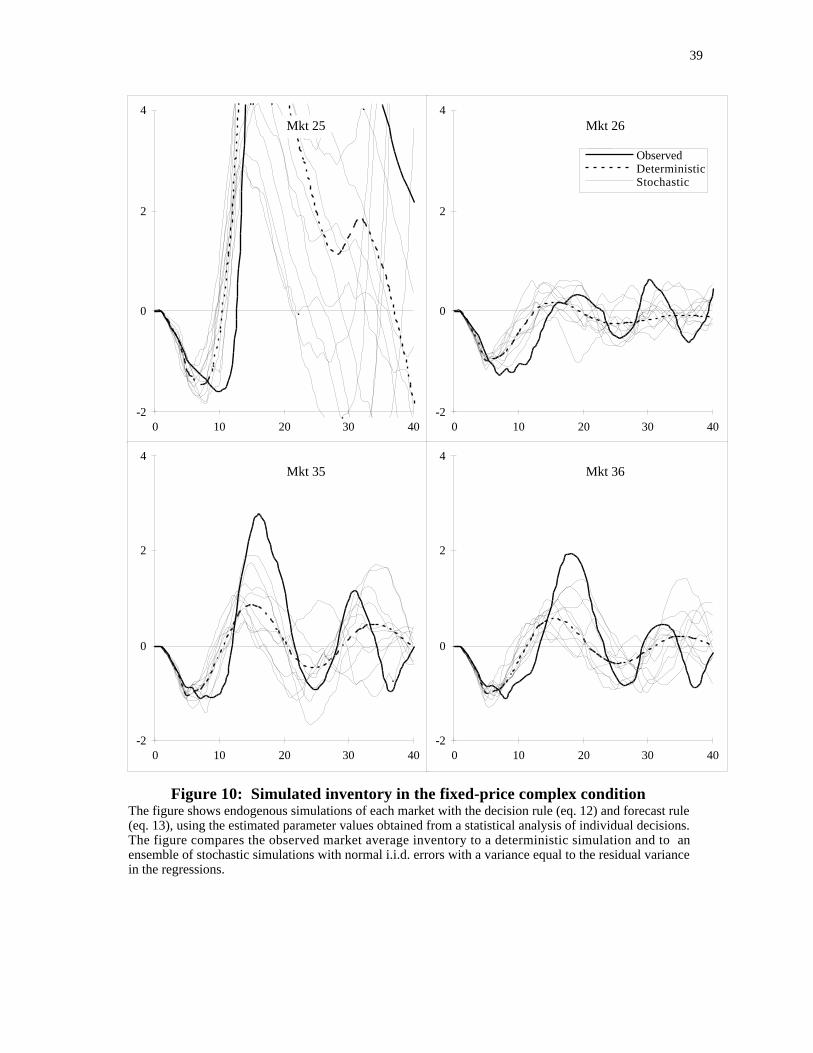
39

-2

0

2

4

0 10 20 30 40

Mkt 25

-2

0

2

4

0 10 20 30 40

Mkt 26

-2

0

2

4

0 10 20 30 40

Mkt 35

-2

0

2

4

0 10 20 30 40

Mkt 36

ObservedDeterministicStochastic

Figure 10: Simulated inventory in the fixed-price complex conditionThe figure shows endogenous simulations of each market with the decision rule (eq. 12) and forecast rule(eq. 13), using the estimated parameter values obtained from a statistical analysis of individual decisions.The figure compares the observed market average inventory to a deterministic simulation and to anensemble of stochastic simulations with normal i.i.d. errors with a variance equal to the residual variancein the regressions.

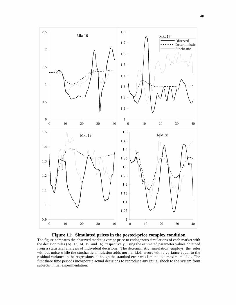
40

0

0.5

1

1.5

2

2.5

0 10 20 30 40

Mkt 16

1

1.1

1.2

1.3

1.4

1.5

1.6

1.7

1.8

0 10 20 30 40

ObservedDeterministicStochastic

Mkt 17

0.9

1

1.1

1.2

1.3

1.4

1.5

0 10 20 30 40

Mkt 18

1

1.05

1.1

1.15

1.2

1.25

1.3

1.35

1.4

1.45

1.5

0 10 20 30 40

Mkt 38

Figure 11: Simulated prices in the posted-price complex conditionThe figure compares the observed market-average price to endogenous simulations of each market withthe decision rules (eq. 13, 14, 15, and 16), respectively, using the estimated parameter values obtainedfrom a statistical analysis of individual decisions. The deterministic simulation employs the ruleswithout noise while the stochastic simulation adds normal i.i.d. errors with a variance equal to theresidual variance in the regressions, although the standard error was limited to a maximum of .1. Thefirst three time periods incorporate actual decisions to reproduce any initial shock to the system fromsubjects' initial experimentation.

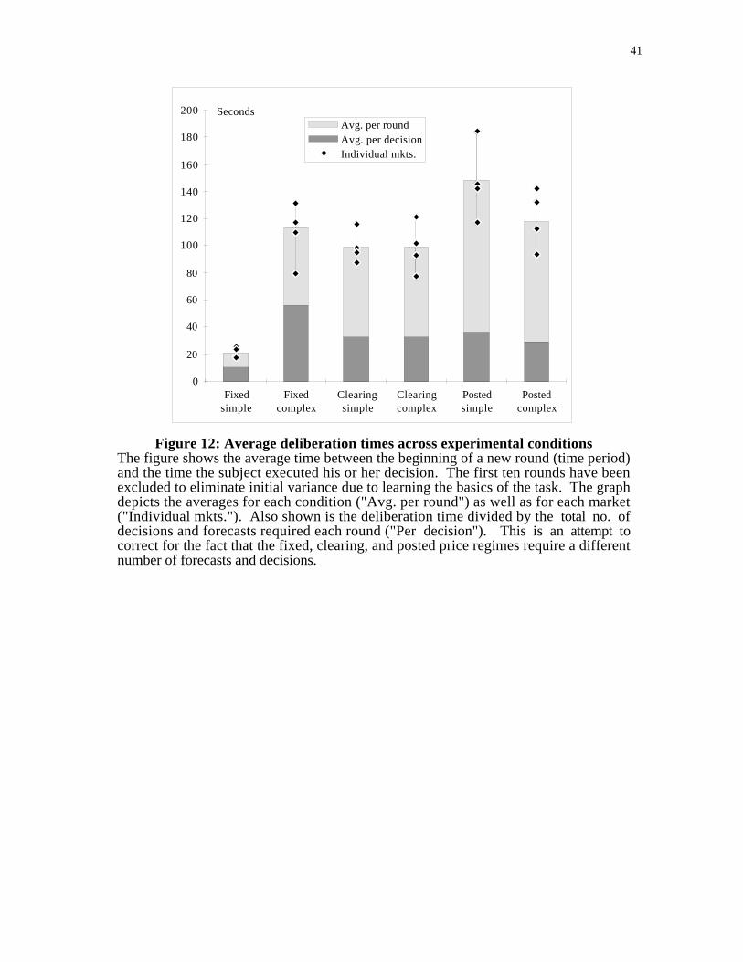
41

0

20

40

60

80

100

120

140

160

180

200

Fixedsimple

Fixedcomplex

Clearingsimple

Clearingcomplex

Postedsimple

Postedcomplex

Avg. per roundAvg. per decisionIndividual mkts.

Seconds

Figure 12: Average deliberation times across experimental conditionsThe figure shows the average time between the beginning of a new round (time period)and the time the subject executed his or her decision. The first ten rounds have beenexcluded to eliminate initial variance due to learning the basics of the task. The graphdepicts the averages for each condition ("Avg. per round") as well as for each market("Individual mkts."). Also shown is the deliberation time divided by the total no. ofdecisions and forecasts required each round ("Per decision"). This is an attempt tocorrect for the fact that the fixed, clearing, and posted price regimes require a differentnumber of forecasts and decisions.