Theoretical Computer Science 507 (2013) 41–51

Contents lists available at ScienceDirect

Theoretical Computer Science

journal homepage: www.elsevier.com/locate/tcs

Feedback vertex sets on restricted bipartite graphs

Wei Jiang a, Tian Liu a,∗, Chaoyi Wang a, Ke Xu b,∗∗

a Key Laboratory of High Confidence Software Technologies, Ministry of Education, Institute of Software, School of Electronic Engineering and Computer Science,Peking University, Beijing 100871, Chinab National Lab of Software Development Environment, Beihang University, Beijing 100191, China

a r t i c l e i n f o

Keywords:Feedback vertex setTree convex bipartitePolynomial timeN P -complete

a b s t r a c t

A feedback vertex set (FVS) in a graph is a subset of vertices whose complement inducesa forest. Finding a minimum FVS is N P -complete on bipartite graphs, but tractable onconvex bipartite graphs and on chordal bipartite graphs. A bipartite graph is called treeconvex, if a tree is defined on one part of the vertices, such that for every vertex in theother part, its neighborhood induces a subtree. When the tree is a path, a triad or a star, thebipartite graph is called convex bipartite, triad convex bipartite or star convex bipartite,respectively. We show that: (1) FVS is tractable on triad convex bipartite graphs; (2) FVS isN P -complete on star convex bipartite graphs and on tree convex bipartite graphs wherethe maximum degree of vertices on the tree is at most three.

© 2012 Elsevier B.V. All rights reserved.

1. Introduction

A feedback vertex set (FVS), sometimes also called a loop cutset [3], in a graph is a subset of vertices whose removalrenders the remaining graph cycle-free [16]. In a weighted graph, the weight of an FVS is the summation of weights over thevertices in the FVS, and the weight of each vertex is a positive integer. For unweighted graphs, each vertex has a unit weight.Finding theminimumweighed FVS (MWFVS, in short) even in unweighted graphs is a classicalN P -complete problem [16],among the twenty-one N P -complete problems in Karp’s list [24]. MWFVS has many applications in deadlock preventionand recovery in operating systems [34], information security [20], VLSI chip design [12], artificial intelligence [2,38], etc.Many algorithms have been developed for MWFVS, such as approximate algorithms [4,2,6,7,33,41], randomized algorithms[3], parameterized algorithms [10,11,8], exact algorithms [14], polynomial algorithms in restricted graphs [29–31,15,9,27,37,21,17,26,25], algorithms to enumerate and count the number of MWFVS [13], and also there are works to estimate thesize ofMWFVS [32,22]. A good survey on tractability ofMWFVS in various graph classes aswell as on various kinds ofMWFVSalgorithms is [12]. A recent good introduction is in [25].

It was known that MWFVS is also N P -complete on unweighed bipartite graphs [39], but tractable on convex bipartitegraphs [29] and on chordal bipartite graphs [25]. A natural question is

• Where is the boundary between tractability and intractability of MWFVS on bipartite graphs?

In this paper, we make partial progress on this question. We investigate MWFVS on tree convex bipartite graphs, whichare generalizations to convex bipartite graphs [19] and chordal bipartite graphs. A bipartite graph G = (A, B, E) is calledtree convex, if a tree T = (A, F) is defined, such that for every vertex b in B, the neighborhood of b induces a subtree in T .

∗ Corresponding author. Tel.: +86 01062765818.∗∗ Corresponding author.

E-mail addresses: lt@pku.edu.cn (T. Liu), kexu@nlsde.buaa.edu.cn (K. Xu).

0304-3975/$ – see front matter© 2012 Elsevier B.V. All rights reserved.doi:10.1016/j.tcs.2012.12.021

42 W. Jiang et al. / Theoretical Computer Science 507 (2013) 41–51

Tree convex bipartite graphs are recognizable in linear time, and the associated tree T is constructible in linear time [40],so we can safely assume that T is a part of the input. For T a path or a star (i.e. a bipartite complete graph K1,|A|−1), G iscalled convex bipartite or star convex bipartite, respectively. For T a triad (i.e. three paths with a common end), G is calledtriad convex bipartite. We show that WMFVS is tractable on triad convex bipartite graphs, but N P -complete on star convexbipartite graphs and on tree convex bipartite graphs with ∆T = 3 where ∆T is the maximum degree of vertices in T . Theseresults refine both the known tractability [29] and intractability [39] results of MWFVS on bipartite graphs.

Both the tree convex bipartite graphs and the chordal bipartite graphs are generalizations to the convex bipartite graphs.The MWFVS algorithm on chordal bipartite graphs in [25] is quite different from the MWFVS algorithm on convex bipartitegraphs in [29] and from ours on triad convex bipartite graphs. So it is interesting to compare chordal bipartite graphs withtree convex bipartite graphs and to see if the algorithm in [25] is extensible to a larger subclass of tree convex bipartitegraphs. It was known that chordal bipartite graphs are subset of tree convex bipartite graphs, but in different context andin different terminologies [1,28]. We give a proof of this fact here, and we also show that the containment is proper. It is anopen problem whether the algorithm in [25] is extensible to a larger subclass of tree convex bipartite graphs.

The results in this paper originally appeared in [22,23,36]. Some similar results for theminimum independent dominatingsets problem were in [35]. Since our works were inspired by [29] and [40], we used the term tree convex bipartite graphsin [22,23,35,36]. What we call tree convex bipartite might also be called hypertree bipartite, tree bipartite, or even subtreebipartite, since the terms hypertree [5], tree-hypergraph [28] and tree convex [40] describe the same family of set systems orhypergraphs.

The remaining part of this paper is organized as follows. The tractability of WMFVS on triad convex bipartite graphs isshown in Section 2. The intractability of MWFVS on star convex bipartite graphs and on tree convex bipartite graphs with∆T = 3 is shown in Section 3. Conclusions and futurework are discussed in Section 4. The proper containment of the chordalbipartite graphs in the tree convex bipartite graphs is discussed in Appendix.

2. Tractability of WMFVS on triad convex bipartite graphs

Recall that removing an FVS renders the remaining graph a forest. Thus finding an MWFVS in a graph is equivalent tofinding a maximum weighted cycle-free set (MWCFS) in the same graph [29]. Below we will extend the algorithm findingMWCFS instead ofMWFVS on convex bipartite graphs in [29] to work onweighted triad convex bipartite graphs. Alongwiththe description, we will also show the correctness of the extended algorithm.

Assume a convex bipartite graph G = (A, B, E), A = {a1, . . . , an}, B = {b1, . . . , bm}, with a linear ordering ai < aj fori < j on A. For convenience, we add two more vertices a0 and an+1 to A [29]. The following notations are from [29]:

• For a vertex v in a graph, N(v) denotes the set of all vertices adjacent to v.• For every b ∈ B in G, let L[b] and R[b] denote the smallest and largest vertices, respectively, of A connected to b. Let

B = {b1, . . . , bm} with R[bi] < R[bj] for 1 ≤ i < j ≤ m.• For ai ∈ Awhere 0 ≤ i ≤ n + 1, let Ai = {ah : ah ∈ A and 0 ≤ h ≤ i} and Bi = {b : b ∈ B and R[b] < ai}.• For ai, aj, ak ∈ A where 0 ≤ i < j < k ≤ n + 1, define Bi,j = {b : b ∈ B and ai < L[b] ≤ R[b] < aj}, and

Bi,j,k = {b : ai < L[b] and aj ≤ R[b] < ak}.• For ai, aj ∈ Awhere i < j,M(i, j) denotes an MWCFS in Aj + Bj containing {ai, aj}( i.e. ai, aj ∈ M(i, j)), where ai and aj are

the largest two vertices in A ∩ M(i, j).• For ai, aj, ak ∈ A where 0 ≤ i < j < k ≤ n + 1, M(i, j, k) denotes an MWCFS in Ak + Bk containing {ai, aj, ak}, where

ai, aj, ak are the largest three vertices in A ∩ M(i, j, k).• For ai, aj ∈ A and bk ∈ Bwhere 0 < i < j < n+ 1 and bk ∈ N(ai) ∩ N(aj),Mb(i, j, k) denotes an MWCFS in Aj + Bj + {bk}

containing {ai, aj, bk}, where ai and aj are the largest two vertices in A ∩ Mb(i, j, k).

In [29], it was shown that all theM(i, j),M(i, j, k) andMb(i, j, k) can be computed inO(|A|3+|A|

2|E|) time. A convex bipartite

graph with the added vertices a0 and an+1 is shown in Fig. 1.Now assume a triad convex bipartite graph G = (A, B, E) with a triad T = (A, F) defined on A, such that every N(b) is

a subtree of T for b ∈ B. To be specific, let A = {a0} ∪ A1 ∪ A2 ∪ A3, such that for 1 ≤ i ≤ 3, Ai = {ai,1, . . . , ai,ni} anda0 → ai,1 → · · · → ai,ni are three paths with a common end a0. The vertices of a triad convex bipartite graph (withoutedges) are shown in Fig. 2.

Let U be the MWCFS of G, we will consider the following two cases: a0 /∈ U and a0 ∈ U .Case 1: a0 /∈ U .Let a1,i, a2,j, a3,k be the nearest vertices to a0 in U on each path A1, A2, A3 respectively. Some of themmay not exist at all,

that is, the corresponding whole path may not intersect with U . We can divide A into four parts S0, S1, S2, S3 as follows:S0 = {a0, a1,1, . . . , a1,i−1, a2,1, . . . , a2,j−1, a3,1, . . . , a3,k−1},S1 = {a1,i, . . . , a1,n1},S2 = {a2,j, . . . , a2,n2},S3 = {a3,k, . . . , a3,n3}.

An example is shown in Fig. 3. Note that if some vertices in {a1,i, a2,j, a3,k} do not exist, then the corresponding sets in{S1, S2, S3} will be empty, however this will cause no harms to our algorithm but only helps.

W. Jiang et al. / Theoretical Computer Science 507 (2013) 41–51 43

Fig. 1. A convex bipartite graph.

Fig. 2. A triad convex bipartite graph (without edges).

Fig. 3. Divide A into four parts.

We can put each v ∈ B into one of the following six sets B1, . . . , B6 according to the situation of v’s neighborhood:B1 = {v | a1,i, a2,j ∈ N(v), a3,k /∈ N(v)}.B2 = {v | a1,i, a3,k ∈ N(v), a2,j /∈ N(v)}.B3 = {v | a2,j, a3,k ∈ N(v), a1,i /∈ N(v)}.B4 = {v | a1,i, a2,j, a3,k ∈ N(v)}.B5 = {v | a1,i, a2,j, a3,k /∈ N(v),N(v) ⊆ S0}.B6 = {v | |{a1,i, a2,j, a3,k} ∩ N(v)| ≤ 1, and N(v) ∩ (S1 ∪ S2 ∪ S3) = ∅}.

44 W. Jiang et al. / Theoretical Computer Science 507 (2013) 41–51

Fig. 4. The vertex sets (without edges) of subgraphs G0,G1,G2,G3 .

The following observations are easily seen.(1) At most one vertex from B1 is selected into U (similarly for B2, B3, B4). Otherwise, if both bp, bq ∈ U are from B1,

then U will contain a cycle bp → a1,i → bq → a2,j → bp. Let b1, b2, b3, b4 be the vertices possibly selected into U fromB1, B2, B3, B4 respectively. Some of them may not exist, since they are not selected into U at all, see below.

(2) Atmost two vertices in {b1, b2, b3} or atmost one vertex in {b4} are available in anyMWCFS, since {b1, b2, b3}will forma cycle b1 → a1,i → b2 → a3,k → b3 → a2,j → b1, and for example {b1, b4}will form a cycle b1 → a1,i → b4 → a2,j → b1.

(3) All the vertices from B5 should be in U , since obviously they are not contained in any cycle.(4) All the edges between B6 and S0 are removable, since they do not change the result of MWCFS.Obviously, the selection of a1,i, a2,j, a3,k is done in at most O(|A|

3) time. According to the above observations (1) and (2),we can enumerate the vertices b1, b2, b3, b4 in O(|B|2) time.

After selecting a1,i, a2,j, a3,k and b1, b2, b3, b4 as above, by the above observation (1), we can remove all vertices in Bi \{bi}from G. After the removing, we define four induced subgraphs G0, G1, G2, G3 of G and find MWCFS in G1, G2, G3 as follows(also see Fig. 4). For any bipartite graph G = (A, B, E) and any subsets C ⊆ A and D ⊆ B, denote by G[C,D] the subgraph ofG induced by C and D, which is the bipartite graph (C,D, E ∩ (C&D)). Here C&D = {(c, d)|c ∈ C and d ∈ D} is the set of allunordered pairs of vertices in C and D. Let N(C) = {b|b ∈ B and b has a neighbor c ∈ C}. Then the graphs G0,G1,G2,G3 aredefined as G[S0,N(S0)], G[S1,N(S1)], G[S2,N(S2)], G[S3,N(S3)] respectively. An example of the vertex sets of subgraphs G0,G1, G2, G3 is shown in Fig. 4.

Let U1, U2, U3 be MWCFS of G1, G2, G3 respectively. It is obvious that U = U1 ∪ U2 ∪ U3 ∪ B5. Let X1 = {v|v ∈

{b1, b2, b4}, v is actually selected into U}. By the observation above (2), we know that |X1| ≤ 2. Below we will show how tofind the MWCFS U1 in G1 conditioned on X1 (we can find U2,U3 in G2,G3 similarly).

Assume that |S1| = n′

1. For convenience, we add two isolated vertices a′

0, a′

n′1+1 into S1 and make an ordering on N(S1) as

in [29]. For the purposes to deal with U2,U3 in a similar way to U1 and to use the algorithm in [29], we rename the verticesin S1 as a′

0, a′

1, . . . , a′

n′1+1 and rename S1,N(S1),G1,U1, X1, n′

1 as A, B,H,U, X, n respectively. Also for convenience, we will

omit the primes in a′

i ’s and b′

j ’s, and use ai’s and bj’s instead in the following lemma. This renaming procedure is partiallydepicted in Fig. 5.Lemma 1. The MWCFS U of H is computed in the following three cases accordingly:1. If X = ∅, U = M(n, n + 1) \ {a0, an+1}.2. If X = {x1}, U is one of the following candidates, whichever has maximum weight:

(a) Mb(i, n, x1) ∪ Bi,n,n+1 \ {a0}, for some i, ai ∈ N(x1).(b) M(i, n, n + 1) \ {a0}, for some i, ai ∈ A \ N(x1) .

3. If X = {x1, x2} and |N(x2) ∩ A| ≥ |N(x1) ∩ A|, U is one of the following candidates, whichever has maximum weight:(a) Mb(i, n, x2) ∪ Bi,n,n+1 \ {a0}, for some i, ai ∈ (N(x2) \ N(x1)).(b) M(i, n, n + 1) \ {a0}, for some i, ai ∈ A \ N(x2).

Proof. Consider the following three cases.1. X = ∅.

U1 is obviouslyM(n, n + 1) \ {a0, an+1} according to the definition ofM(i, j).2. X = {x1}.

If the largest three vertices is ai, an, an+1, both Mb(i, n, x1) ∪ Bi,n,n+1 \ {a0} (when ai ∈ N(x1)) and M(i, n, n + 1) \ {a0}(when ai ∈ A\N(x1)) are cycle-free, and one of them is theMWCFS ofU according to the definitions ofM(i, j, k),Mb(i, j, k)and Bi,j,k.

W. Jiang et al. / Theoretical Computer Science 507 (2013) 41–51 45

Fig. 5. Renaming vertices and finding U1 in G1 .

Fig. 6. Set S of Case 2.

3. X = {x1, x2} and |N(x2) ∩ A| ≥ |N(x1) ∩ A|.If the largest of the three vertices is ai, an, an+1, ai /∈ |N(x1)∩A|, otherwise U contains a cycle x1 → ai → x2 → an → x1.BothMb(i, n, x2)∪Bi,n,n+1 \ {a0} (when ai ∈ N(x2)\N(x1)) andM(i, n, n+1)−{a0} (when ai ∈ A\N(x2)) are cycle-free,and one of them is the MWCFS of U1 according to the definitions of M(i, j, k),Mb(i, j, k) and Bi,j,k.

This finishes the proof. �

Case 2: a0 ∈ U .Similar to Case 1, let a1,i = a0 and a2,j, a3,k be the nearest vertices to a0 in U on each path A2, A3 respectively. Some of

a2,j, a3,k may not exist at all, that is, the corresponding whole path may not intersect with U . We can also divide A into fourparts S0, S1, S2, S3 as follows:

S0 = {a2,1, . . . , a2,j−1, a3,1, . . . , a3,k−1},S1 = {a0, a1,1, . . . , a1,n1},S2 = {a2,j, . . . , a2,n2},S3 = {a3,k, . . . , a3,n3}.

Also note that some of Si’s maybe empty. An example is shown in Fig. 6.We can put each v ∈ B into one of the following five sets B1, . . . , B5 according to the situation of v’s neighborhood:B1 = {v | a0, a2,j ∈ N(v), a3,k /∈ N(v)}.B2 = {v | a0, a3,k ∈ N(v), a2,j /∈ N(v)}.B3 = {v | a0, a1,i, a2,j ∈ N(v)}.B4 = {v | a1,i, a2,j, a3,k /∈ N(v),N(v) ⊆ S0}.B5 = {v | |{a0, a2,j, a3,k} ∩ N(v)| ≤ 1, and N(v) ∩ (S1 ∪ S2 ∪ S3) = ∅}

Then we will immediately get similar observations and lemmas as in Case 1, so we omit the details here.

46 W. Jiang et al. / Theoretical Computer Science 507 (2013) 41–51

Fig. 7. Gadgets of type I (left) and type II (right).

The main steps of the algorithm above are summarized as Algorithm 1.

Input: A triad convex bipartite graph G = (A, B, E) with triad A = {a0} ∪ A1 ∪ A2 ∪ A3Output: A MWCFS U of G

1: U = ∅.2: Enumerate a1,i ∈ A1 ∪ {a0}, a2,j ∈ A2 and a3,k ∈ A3.3: Assume that a1,i, a2,j and a3,k are the nearest vertices to a0 in U on paths {a0} ∪ A1, A2, A3 respectively. Divide A into

S0, S1, S2, S3, divide B into B1, . . . , B6 (when a1,i = a0) or B1, . . . , B5 (when a1,i = a0) accordingly.4: Enumerate b1 ∈ B1, b2 ∈ B2, b3 ∈ B3, b4 ∈ B4 (when a1,i = a0) or b1 ∈ B1, b2 ∈ B2, b3 ∈ B3 (when a1,i = a0).5: Select at most two from {b1, b2, b3} or at most one from {b4} into U , and remove all other vertices in B1, . . . , B4 (when

a1,i = a0) or select atmost two from {b1, b2} or atmost one from {b3} intoU , and remove all other vertices in B1, . . . , B3(when a1,i = a0).

6: Put B5 into U and remove all edges between S0 and B6 (when a1,i = a0) or put B4 into U and remove all edges betweenS0 and B5 (when a1,i = a0).

7: Define subgraphs G0,G1,G2,G3 accordingly and find the MWCFS U1,U2,U3 in G1,G2,G3 respectively. Update U byU1 ∪ U2 ∪ U3 ∪ B5 (when a1,i = a0) or by U1 ∪ U2 ∪ U3 ∪ B4 (when a1,i = a0).

8: If the enumeration in step 4 is unfinished then goto step 4, else if the enumeration in step 2 is unfinished then gotostep 2.

Algorithm 1: Finding MWFVS in triad convex bipartite graphs.

Theorem 1. An MWFVS in a triad convex bipartite graphs is computable in O(|A|3|B|2(|A|

3+ |A|

2|E|)) time.

Proof. Enumerating a1,i, a2,j, a3,k is done in O(|A|3) and enumerating b1, b2, b3, b4 is done in O(|B|2). So the total

enumeration time is O(|A|3|B|2). According to [29], all M(i, j),M(i, j, k) and Mb(i, j, k) are computed in O(|A|

3+ |A|

2|E|)

time. Therefore, an MWCFS in a triad convex bipartite graph is found in O(|A|3|B|2(|A|

3+ |A|

2|E|)) time. The complement of

this MWCFS is an MWFVS. �

3. Intractability of MWFVS on tree convex bipartite graphs

In this section, we show that the algorithms in [29] and in the last section are unlikely to be extensible to star convexbipartite graphs and to tree convex bipartite graphs with ∆T = 3, unless N P = P .

Theorem 2. MWFVS is N P -hard in unweighed star convex bipartite graphs.

Proof. We give a reduction from the minimum vertex cover (VC) to MWFVS in star convex bipartite graphs. Given anon-trivial (i.e. neither an independent set nor a clique) graph G = (V , E), we construct a star convex bipartite graphG′

= (A, B, E ′), such that VC in graph G is equivalent to MWFVS in graph G′, as follows.Let |A∪B| = 3|V |+2|E|+1. The set A contains |V |+1 vertices a0, a1, . . . , a|V |. For 1 ≤ i ≤ |V |, the vertex ai is called an

external vertex and corresponds exclusively to a vertex vi in V . The vertex a0 is called the central vertex. The set B contains2|V | + 2|E| vertices b1, b2, . . . , b2|V |+2|E|.

Let |E ′| = 4|V | + 6|E|. The graph G′ is composed by two types of gadgets. Gadgets of type I are complete bipartite graphs

K2,2, each with four edges and corresponding exclusively to a vertex in V . Gadgets of type II are complete bipartite graphsK3,2, each with six edges and corresponding exclusively to an edge in E. See Fig. 7. For every vertex vi in V (1 ≤ i ≤ |V |),we build a gadget of type I in G′, which is a K2,2 on four vertices ai, a0, b2i−1, b2i. For every edge ei = (vj, vk) in E(1 ≤ i ≤ |E|, 1 ≤ j, k ≤ |V |), we build a gadget of type II in G′, which is a K3,2 on five vertices aj, ak, a0, b2|V |+2i−1, b2|V |+2i.The construction of graph G′ is finished. An example of G = ({1, 2, 3, 4}, {(1, 2), (1, 3), (1, 4)}) and the construction of G′

is shown in Fig. 8. Clearly, the construction is in polynomial time. The following three lemmas show its correctness.

Lemma 2. The graph G′ is star convex bipartite.

Proof. Both types of gadgets are complete bipartite graphs, with all edges between vertices in A and vertices in B. So G′ is abipartite graph, with all edges between vertices in A and vertices in B.

Both types of gadgets are complete bipartite graphs containing a0. So every vertex b in B is connected to a0. In fact, for1 ≤ i ≤ |V |, the neighborhoods of b2i−1 and b2i are both {a0, ai}. For 1 ≤ i ≤ |E|, the neighborhoods of b2|V |+2i−1 and b2|V |+2i

W. Jiang et al. / Theoretical Computer Science 507 (2013) 41–51 47

Fig. 8. An example of the construction.

are both {a0, aj, ak}, where ei = (aj, ak) is an edge in E. Let the tree T on A be a star with center a0 and leaves a1, . . . , a|V |.Then for 1 ≤ i ≤ |V |, the neighborhoods of b2i−1 and b2i are both a star in T with center a0 and leaf ai. For 1 ≤ i ≤ |E|, theneighborhoods of b2|V |+2i−1 and b2|V |+2i are both a star in T with center a0 and leaves aj, ak. So G′ is also star convex. �

Lemma 3. Graph G has a VC of size no more than k, only if G′ has an FVS of size no more than k + 1.

Proof. We show that given any VC S in graph G, let S ′ be the corresponding vertices in A, then S ′∪ {a0} is an FVS in G′.

By definition of FVS, S ′∪ {a0} is an FVS in G′ if and only if S ′

∪ {a0} covers all cycles in G′. Clearly, each cycle in G′ eithercontains the vertex a0 or contains two vertices aj and ak such that (vj, vk) is an edge in G, see Figs. 7 and 8. To cover an edge(vj, vk) in G, either vj or vk or both should be in S, thus either aj or ak or both should be in S ′. Thus S ′

∪ {a0} covers all cyclesin G′. �

Lemma 4. Graph G has a VC of size no more than k, if G′ has an FVS of size no more than k + 1.

Proof. Assume that S ′ is an FVS in G′. If a0 is not in S ′, then at least one other vertex of every gadget of type I will be in S ′, so|S ′

| ≥ |V |. On the other hand, since G is not a clique, say (vj, vk) is not an edge in E, then V \ {vj, vk} is a VC in G, so G has aVC of size no more than |V | − 2, the lemma trivially holds.

So assume that a0 is in S ′. If S ′ contains any vertex bi in B, then we can select any neighbor of bi other than a0 to replacebi. Still all the cycles in G′ are covered, thus the result is an FVS in G′ and its size is no more than that of S ′. So without lossof generality, we may assume that S ′ is contained in A.

Now let S be the corresponding vertices of S ′\ {a0} in G. We show that S is a VC in G as follows. Otherwise, there is an

edge ei = (vj, vk) not covered by S. So both vj and vk are not in S, and accordingly both aj and ak are not in S ′. Then thecorresponding gadget of type II of ei will contain a cycle aj → b2|V |+2i−1 → ak → b2|V |+2i → aj, which is not covered by S ′.This is a contradiction to the assumption that S ′ is an FVS in G′. �

This finishes the proof of Theorem 2. �

Theorem 3. MWFVS is N P -complete in unweighted tree convex bipartite graphs with ∆T = 3.

Proof. We reduce from VC to MWFVS in the tree convex bipartite graphs with ∆T = 3. Given an unweighed graph G =

(V , E) with n vertices and m edges, where V = {v1, . . . , vn} and E = {e1, . . . , em}, without loss of generality, we mayassume that G is not a complete graph, that is, there is at least one pair of vertices which are not connected by any edge. Wewill construct a tree convex bipartite graph G′

= (A, B, E ′) and a tree T = (A, F) with ∆T = 3, such that for every vertex bin B, the neighborhood of b, N(b) = {v ∈ A|(v, b) ∈ E ′

}, is a subtree on A.The construction will be in four stages. In the first stage, we keep the vertices of graph G unchanged but replace each

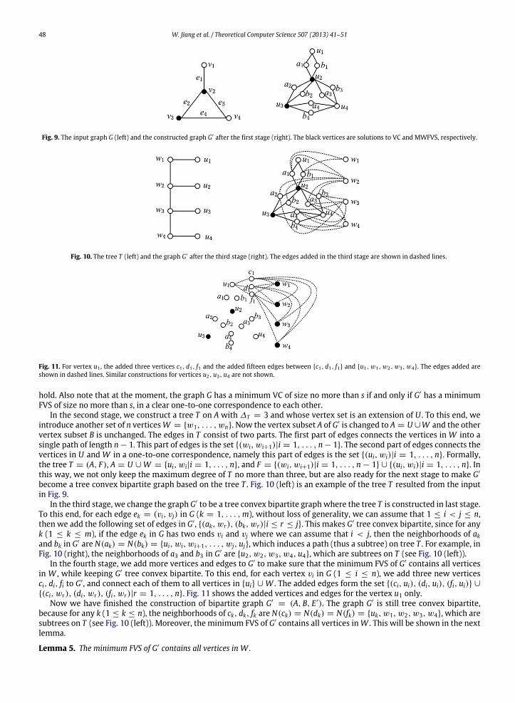
edge of G with two independent paths both of length two. This stage actually reduces VC to MWFVS on general bipartitegraphs. Fig. 9 shows an example of this construction. Formally, after the first stage of the reduction, the constructedgraph G′

= (A, B, E ′) has the following form, A = U = {u1, . . . , un}, B = {ak, bk|ek ∈ E, k = 1, . . . ,m}, andE ′

= {(ui, ak), (ui, bk), (ak, uj), (bk, uj)|ek = (vi, vj) ∈ E, k = 1, . . . ,m}. It is easy to see that, for each edge ek = (vi, vj) inG, the corresponding vertices ak, bk in G′ only appear on a unique cycle ui → ak → uj → bk → ui. Then whenever thereis a vertex ak or bk in a solution to MWFVS in G′, we can safely replace this vertex either by ui or by uj without destroyingthe solution or increasing the size of the solution. Thus, we can assume that the optimal solution of MWFVS in G′ is totallycontained in A and has no intersectionwith B. When the construction is completed in the fourth stage, this property will still

48 W. Jiang et al. / Theoretical Computer Science 507 (2013) 41–51

Fig. 9. The input graph G (left) and the constructed graph G′ after the first stage (right). The black vertices are solutions to VC and MWFVS, respectively.

Fig. 10. The tree T (left) and the graph G′ after the third stage (right). The edges added in the third stage are shown in dashed lines.

Fig. 11. For vertex u1 , the added three vertices c1, d1, f1 and the added fifteen edges between {c1, d1, f1} and {u1, w1, w2, w3, w4}. The edges added areshown in dashed lines. Similar constructions for vertices u2, u3, u4 are not shown.

hold. Also note that at the moment, the graph G has a minimum VC of size no more than s if and only if G′ has a minimumFVS of size no more than s, in a clear one-to-one correspondence to each other.

In the second stage, we construct a tree T on A with ∆T = 3 and whose vertex set is an extension of U . To this end, weintroduce another set of n verticesW = {w1, . . . , wn}. Now the vertex subset A of G′ is changed to A = U ∪W and the othervertex subset B is unchanged. The edges in T consist of two parts. The first part of edges connects the vertices in W into asingle path of length n− 1. This part of edges is the set {(wi, wi+1)|i = 1, . . . , n− 1}. The second part of edges connects thevertices in U and W in a one-to-one correspondence, namely this part of edges is the set {(ui, wi)|i = 1, . . . , n}. Formally,the tree T = (A, F), A = U ∪ W = {ui, wi|i = 1, . . . , n}, and F = {(wi, wi+1)|i = 1, . . . , n − 1} ∪ {(ui, wi)|i = 1, . . . , n}. Inthis way, we not only keep the maximum degree of T no more than three, but are also ready for the next stage to make G′

become a tree convex bipartite graph based on the tree T . Fig. 10 (left) is an example of the tree T resulted from the inputin Fig. 9.

In the third stage, we change the graph G′ to be a tree convex bipartite graphwhere the tree T is constructed in last stage.To this end, for each edge ek = (vi, vj) in G (k = 1, . . . ,m), without loss of generality, we can assume that 1 ≤ i < j ≤ n,then we add the following set of edges in G′, {(ak, wr), (bk, wr)|i ≤ r ≤ j}. This makes G′ tree convex bipartite, since for anyk (1 ≤ k ≤ m), if the edge ek in G has two ends vi and vj where we can assume that i < j, then the neighborhoods of akand bk in G′ are N(ak) = N(bk) = {ui, wi, wi+1, . . . , wj, uj}, which induces a path (thus a subtree) on tree T . For example, inFig. 10 (right), the neighborhoods of a3 and b3 in G′ are {u2, w2, w3, w4, u4}, which are subtrees on T (see Fig. 10 (left)).

In the fourth stage, we add more vertices and edges to G′ to make sure that the minimum FVS of G′ contains all verticesin W , while keeping G′ tree convex bipartite. To this end, for each vertex vi in G (1 ≤ i ≤ n), we add three new verticesci, di, fi to G′, and connect each of them to all vertices in {ui} ∪ W . The added edges form the set {(ci, ui), (di, ui), (fi, ui)} ∪

{(ci, wr), (di, wr), (fi, wr)|r = 1, . . . , n}. Fig. 11 shows the added vertices and edges for the vertex u1 only.Now we have finished the construction of bipartite graph G′

= (A, B, E ′). The graph G′ is still tree convex bipartite,because for any k (1 ≤ k ≤ n), the neighborhoods of ck, dk, fk are N(ck) = N(dk) = N(fk) = {uk, w1, w2, w3, w4}, which aresubtrees on T (see Fig. 10 (left)). Moreover, the minimum FVS of G′ contains all vertices inW . This will be shown in the nextlemma.

Lemma 5. The minimum FVS of G′ contains all vertices in W.

W. Jiang et al. / Theoretical Computer Science 507 (2013) 41–51 49

Proof. Let D be the FVS of G′. We consider the size of D in the following three cases.

• Case 1:W ⊆ D. Since we have assumed that the input graph G is not a complete graph, there is a pair of vertices vi and vjwhich are not connected by any edge. ThenW ∪U \ {ui, uj} is an FVS of G′. This is because when deletingW ∪U \ {ui, uj}

from G′, all cycles created at the first, third and fourth stages in G′ are broken. Since D is the minimum FVS of G′, we havethat |D| ≤ |W | + |U| − 2 = 2n − 2.

• Case 2: (W \ {wi}) ⊆ D and wi ∈ D for some 1 ≤ i ≤ n. In this case, we must have that U ⊆ D. For otherwise, if uj isnot in D for some j (1 ≤ j ≤ n), then the five vertices uj, cj, dj, fj, wi make a complete bipartite graph K2,3 by the fourthstage of the construction. Since neither wi nor uj is in D, to break the cycles in this small K2,3, we have to put at leasttwo of the three vertices cj, dj, fj into D. But this will be a contradiction to the minimum property of D, since instead ofat least two of the three vertices cj, dj, fj, we only need to put one vertex uj into D to break the cycles in this small K2,3.Note that replacing two of the three vertices {cj, dj, fj} by uj will cause no harm to D, since we do not need any vertex in{cj, dj, fj} to break any other cycles. In fact, the other cycles containing {cj, dj, fj} have already been broken by W \ {wi}.Thus, (U ∪ W \ {wi}) ⊆ D and |D| ≥ 2n − 1.

• Case 3: |W \ D| ≥ 2. Assume that neither wi nor wj is in D for some 1 ≤ i ≤ j ≤ n. Then for each uk (1 ≤ k ≤ n), the fivevertices ck, dk, fk, wi, wj make a small complete bipartite graph K2,3. To break the cycles in this K2,3, D has to contain atleast two of the three vertices ck, dk, fk. This holds for each k (1 ≤ k ≤ n). Thus |D| ≥ 2n.

Since D is an FVS in G′ with minimum cardinality, we conclude that the above Case 1 must be true, namelyW ⊆ D. �

Now the correctness of the reduction is shown by the following two lemmas.

Lemma 6. If G has a VC of size no more than s, then G′ has an FVS of size no more than s + n.

Proof. Let S be a VC in G of size no more than s, then {ui|vi ∈ S} ∪ W is an FVS in G′ of size no more than s + n. Indeed, allthe cycles created at the first stage are broken by {ui|vi ∈ S} (see the discussions at the end of the description of the firststage), and all the cycles created at the third and fourth stages are broken byW . �

Lemma 7. If G′ has an FVS of size no more than s + n, then G has a VC of size no more than s.

Proof. Assume that D is the minimum FVS in G, then |D| ≤ s + n. By the Lemma 7, we have that W ⊆ D. All the cyclescreated at the third and fourth stages are broken byW . By the discussions in the first stage, all the cycles created at the firststages can be broken by vertices in U , instead of by any vertices in {ak, bk|k = 1, . . . ,m}, without increasing the size of theFVS. Thus, we can assume that D ⊆ (U ∪ W ) = A. Then the set S = {vi|ui ∈ D \ W } is a VC in G of size no more than s. Forotherwise, there is an edge ek = (vi, vj) in G but neither of vi and vj is in S. By the definition of S, we have that neither of uiand uj is in D. We have already assumed that neither of ak and bk is in D. Thus, the cycle ui → ak → uj → bk → ui in G′ isnot broken by D, a contradiction to the fact that D is an FVS. �

The proof of this theorem is finished. �

4. Conclusion and future work

We have extended the MWFVS algorithm on convex bipartite graphs in [29] to a polynomial time MWFVS algorithm ontriad convex bipartite graphs, and shown that MWFVS is N P -complete on star convex bipartite graphs and on tree convexbipartite graphs where the maximum degree of vertices in the tree is three. It would be interesting to extend our algorithmand the algorithm in [25] to a larger subclass of tree convex bipartite graphs.

Appendix. Chordal bipartite graphs versus tree convex bipartite graphs

Chordal bipartite graphs were introduced in [18] and have been extensively studied since then [5,25]. A chord of a cycleon a graph is an edge between two vertices of the cycle but the edge itself is not a part of the cycle. A graph (not necessarilybipartite) is chordal if every cycle of length at least four has a chord. A bipartite graph is chordal bipartite if every cycle oflength at least six has a chord. Note that in general chordal bipartite graphs are not chordal. We refer to [5,25] for differentequivalent definitions of chordal bipartite graphs.

Theorem 4. There is a bipartite graph which is tree convex but not chordal bipartite.

Proof. The bipartite graph G is shown in Fig. A.12 (left). G is not chordal bipartite, because the cycle axbzcya has no chord.G is tree convex bipartite, because the neighborhoods of a, b, c are N(a) = {x, y, w}, N(b) = {x, z, w} and N(c) = {z, y, w},respectively. If we define a tree T on vertices {x, y, z, w}, which is a star with the center w and three leaves x, y, z, thenN(a) = {x, y, w} is a subtree of T , as shown in Fig. A.12 (right). For N(b) and N(c), the situations are similar. �

The containment of chordal bipartite graphs in tree convex bipartite graphs was known before [1,28], and weindependently gave a proof in [36]. Since the proofs in [1,28] were either in a different context or in different terminologies,we list our proof as the following theorem, which we believe essentially the same as in [28] but in a more explicit form.

50 W. Jiang et al. / Theoretical Computer Science 507 (2013) 41–51

Fig. A.12. The bipartite graph G and the tree T .

Theorem 5. Every chordal bipartite graph is tree convex bipartite.

Proof. Let G = (A, B, E) be a chordal bipartite graph. From G, we can define a new hypergraph H and a new graph L(H)respectively as follows.

First, we define H . For each vertex b in B, its neighborhood N(b) = {a ∈ A|(a, b) ∈ E} is a subset of A. The set system Econtains all these neighborhoods of vertices in B, namely E = {N(b)|b ∈ B}. The hypergraph H is defined as H = (A, E). Thevertex set of H is A and each N(b) is a hyperedge of H . When G is chordal, we can show that H has the Helly property. A setsystem E has theHelly property, if for any subsystem E ′ of E , whenever the sets in E ′ have non-empty pairwise intersections,then all sets in E have a common element ([5], p. 8, Definition 1.3.4). If E has the Helly property, then H = (A, E) is called aHelly hypergraph.

Lemma 8. If G = (A, B, E) is chordal bipartite, then H = (A, E) is a Helly hypergraph.

Proof. Let E ′ be a subsystem of E . Assume that any two subsets of E ′ have a non-empty intersection. We will show that allsets in E ′ have a common element. We do induction on the cardinality of E ′.

The base step. If E ′ has three sets N(b1), N(b2), N(b3), and a1 ∈ N(b2)∩N(b3), a2 ∈ N(b1)∩N(b3), a3 ∈ N(b1)∩N(b2). Ifany two of a1, a2, a3 are the same, then we have a common element in N(b1), N(b2), N(b3). If a1, a2, a3 are all distinct, thena1b2a3b1a2b3a1 is a cycle of length six in G. Since G is chordal bipartite, the cycle has a chord, say (ai, bi) (1 ≤ i ≤ 3). Thenai is a common element of sets in E ′.

The induction step. Assume that for all E ′ of cardinality no more than k (k ≥ 3) in which sets are pairwise intersecting,all sets in E ′ has a common element. We show that for E ′ of cardinality k + 1 in which sets are pairwise intersecting, allsets in E ′ has a common element. Assume that E ′

= {N(bi)|i = 1, 2, . . . , k + 1}. Let S =

{N(bi)|i = 3, . . . , k + 1}.By the induction hypothesis, N(b1) ∩ S = ∅, N(b2) ∩ S = ∅. By the assumption on E ′, N(b1) ∩ N(b2) = ∅. Similarly, leta1 ∈ N(b2) ∩ S, a2 ∈ N(b1) ∩ S, a3 ∈ N(b1) ∩ N(b2). Suppose that a1, a2, a3 are all distinct, then we have k − 1 cycles oflength 6, that is a1b2a3b1a2bia1, i = 3, . . . , k+1. If a1 ∈ N(b1) or a2 ∈ N(b2), then S,N(b1),N(b2) have a common element.If a1 ∈ N(b1) and a2 ∈ N(b2), then all the cycles must have chords a3bi. Hence a3 ∈ N(bi), i = 3, . . . , k + 1. By definition ofS, we obtain a3 ∈ S. Thus, S,N(b1),N(b2) always have a common element, which in turn is a common element of sets in E ′.The induction is finished.

Thus H is a Helly hypergraph. �

Next, we define graph L(H) = (E, F ), the line graph or intersection graph of H ([5], p. 7–8, Definition 1.3.3), whereF = {(N(bi),N(bj))|N(bi) ∩ N(bj) = ∅, bi, bj ∈ B}. We will show that L(H) is chordal.

Lemma 9. If G = (A, B, E) is chordal bipartite, then L(H) = (E, F ) is chordal.

Proof. Assume that N(b1)N(b2) · · ·N(bk)N(b1) is a cycle of length k (k ≥ 4) in L(H). By the definition of L(H), there area1, . . . , ak in A, such that ai ∈ N(bi) ∩ N(bi+1) for i = 1, . . . , k − 1 and ak ∈ N(bk) ∩ N(b1). If all these ai’s are all distinct,then b1a1b2a2 · · · bkakb1 is a cycle in G of length at least eight. Since G is chordal bipartite, there is a chord for this cycle of G,say (ai, bj) (1 ≤ i, j ≤ k), then (N(bi),N(bj))will be a chord for the cycle of L(H). If some of the ai’s are the same, say ai = aj,then (N(bi),N(bj+1)) will be a chord for the cycle of L(H). Thus L(H) is chordal. �

A hypergraph H is called a hypertree, if there is a tree T with the same vertices of H , such that all hyperedges inducesubtrees in T ([5], p. 8–9, Definition 1.3.6). A hypergraph H is a hypertree, if and only if H has the Helly property and its linegraph L(H) is chordal ([5], p. 9, Theorem 1.3.1). Thus, by above two lemmas, the graph H defined from the chordal bipartiteG is a hypertree. But H is a hypertree is equivalent to that G is a tree convex bipartite graph, by definitions. �

Acknowledgments

We thank Professor Kaile Su for encouragements and supports. This research was partially supported by National 973Program of China (grant 2010CB328103) and National Natural Science Foundation of China (grant 60973033). We aregrateful to the unknown reviewers for many helpful comments.

W. Jiang et al. / Theoretical Computer Science 507 (2013) 41–51 51

References

[1] R.P. Anstee, Hypergraphs with no special cycles, Combinatorica 3 (1983) 141–146.[2] R. Bar-Yehuda, D. Geiger, J. Naor, R. Roth, Approximation algorithms for the feedback vertex set problem with applications to constraint satisfaction

and Bayesian inference, SIAM J. Comput. 27 (1998) 942–959.[3] A. Becker, R. Bar-Yehuda, D. Geiger, Randomized algorithms for the loop cutset problem, J. Artif. Intell. Res. 12 (2000) 219–234.[4] A. Becker, D. Geiger, Optimization of Pearls method of conditioning and greedy-like approximation algorithms for the vertex feedback set problem,

Artificial Intelligence 83 (1996) 167–188.[5] A. Brandstad, V.B. Le, J.P. Spinrad, Graph Classes—A Survey, Society for Industrial and Applied Mathematics, Philadelphia, 1999.[6] M. Cai, X. Deng, W. Zang, An approximation algorithm for feedback vertex sets in tournaments, SIAM J. Comput. 30 (2001) 1993–2007.[7] M. Cai, X. Deng, W. Zang, A min–max theorem on feedback vertex sets, Math. Oper. Res. 27 (2) (2002) 361–371.[8] Y. Cao, J. Chen, Y. Liu, On feedback vertex set: new measure and new structures, in: Proc of SWAT, in: LNCS, vol. 6139, 2010, pp. 93–104.[9] I. Caragiannis, C. Kaklamanis, P. Kanellopoulos, New bounds on the size of the feedback vertex set on meshes and butterflies, Inform. Process. Lett. 83

(5) (2002) 275–280.[10] J. Chen, F. Fomin, Y. Liu, S. Lu, T. Villanger, Improved algorithms for feedback vertex set problems, J. Comput. System Sci. 74 (7) (2008) 1188–1198.[11] J. Chen, Y. Liu, S. Lu, B. O’Sullivan, I Razgon, A fixed-parameter algorithm for the directed feedback vertex set problem, J. ACM 55 (5) (2008).[12] P. Festa, P.M. Pardalos, M.G.C. Resende, Feedback set problems, in: D.-Z. Du, P.M. Pardalos (Eds.), Handbook of Combinatorial Optimization, Kluwer

Academic Publishers, 2000, pp. 209–259. Supplement vol. A.[13] F.V. Fomin, S. Gaspers, A. Pyatkin, I. Razgon, On the minimum feedback vertex set problem: exact and enumeration algorithms, Algorithmica 52 (2)

(2008) 293–307.[14] F.V. Fomin, Y. Villanger, Finding induced subgraphs via minimal triangulations. Proc. of STACS 2010, pp. 383–394.[15] R. Focardi, F.L. Luccio, D. Peleg, Feedback vertex set in hypercubes, Inform. Process. Lett. 76 (1–2) (2000) 1–5.[16] M.R. Garey, D.S. Johnson, Computers and Intractability, a Guide to the Theory of NP-Completeness, W.H. Freeman and Company, 1979.[17] F. Gavril, Minimum weight feedback vertex sets in circle graphs, Inform. Process. Lett. 107 (2008) 1–6.[18] M.C. Golumbic, C.F. Goss, Perfect elimination and chordal bipartite graphs, J. Graph Theory 2 (1978) 155–163.[19] F. Grover, Maximummatching in a convex bipartite graph, Nav. Res. Logist. Q. 14 (1967) 313–316.[20] D. Gusfield, A graph theoretic approach to statistical data security, SIAM J. Comput. 17 (3) (1998) 552–571.[21] C.C. Hsu, H.R. Lin, H.C. Chang, K.K. Lin, Feedback vertex sets in rotator graphs, in: Lecture Notes in Comput. Sci., vol. 3984, 2006, pp. 158–164.[22] W. Jiang, T. Liu, T.N. Ren, K. Xu, Two hardness results on feedback vertex sets, in: Proc. of FAW-AAIM 2011, 2011, pp. 233–243.[23] W. Jiang, T. Liu, K. Xu, Tractable feedback vertex sets in restricted bipartite graphs, in: Proc. of COCOA 2011, 2011, pp. 424–434.[24] R. Karp, Reducibility among combinatorial problems, in: Complexity of Computer Computations, Plenum Press, New York, 1972, pp. 85–103.[25] T. Kloks, C.H. Liu, S.H. Poon, Feedback vertex set on chordal bipartite graphs, 2011, ArXiv:1104.3915.[26] C. Kuo, C. Hsu, H. Lin, K. Lin, An efficient algorithm for minimum feedback vertex sets in rotator graphs, Inform. Process. Lett. 109 (2009) 450–453.[27] R. Kralovic, P. Ruzicka, Minimum feedback vertex sets in shufflebased interconnection networks, Inform. Process. Lett. 86 (4) (2003) 191–196.[28] J. Lehel, A characterization of totally balanced hypergraphs, Discrete Math. 57 (1985) 59–65.[29] Y.D. Liang, M.S. Chang, Minimum feedback vertex sets in cocomparability graphs and convex bipartite graphs, Acta Inform. 34 (1997) 337–346.[30] C. Lu, C. Tang, A linear-time algorithm for the weighted feedback vertex problem on interval graphs, Inform. Process. Lett. 61 (1997) 107–111.[31] F.L. Luccio, Exact minimum feedback vertex set in meshes and butterflies, Inform. Process. Lett. 66 (2) (1998) 59–64.[32] F.R. Madelaine, I.A. Stewart, Improved upper and lower bounds on the feedback vertex numbers of grids and butterflies, Discrete Math. 308 (2008)

4144–4164.[33] P. Sasatte, Improved approximation algorithm for the feedback set problem in a bipartite tournament, Oper. Res. Lett. 36 (2008) 602–604.[34] A. Silberschatz, P.B. Galvin, G. Gagne, Operating Systems Concepts, 6th ed., John Wiley and Sons, Inc., New York, 2003.[35] Y. Song, T. Liu, K. Xu, Independent domination on tree convex bipartite graphs, in: Proc. of FAW-AAIM 2012, 2012, pp. 129–138.[36] C. Wang, T. Liu, W. Jiang, K. Xu, Feedback vertex sets on tree convex bipartite graphs, in: Proc. of COCOA 2012, 2012, pp. 95–102.[37] F.H. Wang, Y.L. Wang, J.M. Chang, Feedback vertex sets in star graphs, Inform. Process. Lett. 89 (4) (2004) 203–208.[38] R. Williams, C.P. Gomes, B. Selman, Backdoors to typical case complexity, in: Proc. of IJCAI 2003, pp. 1173–1178.[39] M. Yannakakis, Node-deletion problem on bipartite graphs, SIAM J. Comput. 10 (1981) 310–327.[40] Y. Zhang, F.S. Bao, A review of tree convex sets test, Computational Intelligence 28 (3) (2012) 358–372. Old version: A survey of tree convex sets test,

2009. ArXiv:0906.0205.[41] A. van Zuylen, Linear programming based approximation algorithms for feedback set problems in bipartite tournaments, Theoret. Comput. Sci. 412

(23) (2011) 2556–2561.