CERIAS Tech Report 2001-24

Femotosecond Direct Space-to-Time Pulse Shaping

D.E. Leaird, A.M. Weiner

Center for Education and Research in Information Assurance and Security

& School of Electrical & Computer Engineering, Purdue University

West Lafayette, IN 47907

CERIAS TR 2001-24

1 of 25

Abstract—The Direct Space-to-Time pulse shaping apparatus is investigated both theoretically

and experimentally. The discussion shows how the operation of the DST pulse shaper may be understood

in terms of the femtosecond response of a generalized spectrometer. A complete discussion of the

advantages and trade-offs of utilizing this pulse shaping configuration is given including the direct scaling

between the masking function and the output temporal intensity profile, system efficiency, spectral

resolution, and temporal window, compensation/cancellation of chirp, and generation of multiple output

waveforms.

Index terms—ultrafast optics, pulse shaping

Femtosecond Direct Space-to-Time Pulse

Shaping

D.E. Leaird, and A.M. Weiner, Fellow, IEEE

School of Electrical & Computer Engineering, and Center for Education and Research in Information

Assurance and Security – CERIAS, Purdue University,

1285 Electrical Engineering Bldg., West Lafayette, IN 47907-1285

CERIAS TR 2001-24

2 of 25

I. INTRODUCTION

Pulse shaping methods allowing synthesis of complex femtosecond optical waveforms according

to specification are now well established [1-7]. As usually practiced, the output waveform is determined

by the Fourier transform of a spatial pattern transferred by a mask or a modulator array onto the dispersed

optical spectrum. Such Fourier transform femtosecond pulse shaping is used in many scientific

applications of femtosecond optics, e.g., [8,9], and applications in communications are also being explored

[10-13]. However, for some communications applications, one would prefer a direct (rather than a Fourier

transform) mapping between a spatial pattern and the resultant ultrafast optical waveform. One example is

in parallel-to-serial conversion, where one might envision converting a parallel electronic data word to an

ultrafast optical serial data packet by using a suitable pulse shaping geometry containing an optoelectronic

modulator array driven by the data word. For this purpose it would be desirable that each bit in the output

optical data packet be associated with a single modulator element, both for simplicity and because the need

to compute a Fourier transform before setting the state of the modulator array would restrict operation to

relatively low packet rates.

Such a pulse shaping geometry, which we call the direct space-to-time (DST) pulse shaper, was

previously demonstrated for relatively simple pulse shapes with pulse duration's in the several picosecond

range [14]-[17]. In recent work we demonstrated the first operation of a DST pulse shaper for generation

of femtosecond data packets [18] and developed a means for controlling the chirp in the DST pulse shaper

[19], which would be important for subsequent transmission over optical fibers. In this paper we give a

comprehensive discussion of the DST pulse shaper on a femtosecond time scale and present a number of

new results, including a method for simultaneous generation of multiple wavelength-shifted but otherwise

identical pulse sequences from the DST pulse shaper and a generalization of our previous chirp control

results. Furthermore, we show how the operation of the DST pulse shaper may be understood as the

femtosecond response of a generalized spectrometer.

The remainder of this paper is structured as follows. Section II contains an analysis of the DST

pulse shaper under a relatively simple set of conditions and describes how the basic direct space-to-time

conversion function may be understood by analogy with a simple spectrometer. Section III discusses the

experimental apparatus and presents results demonstrating direct space-to-time conversion for both simple

CERIAS TR 2001-24

3 of 25

and highly structured optical waveforms. Tradeoffs between spectral resolution, temporal window, and

efficiency are also analyzed in this section. The first complete analysis of the chirp compensation

properties of the DST shaper, including experimental confirmation of this analysis, is presented in Section

IV. These results show that the chirp behavior of the DST shaper is rather different than the well-known

chirp behavior of Fourier transform pulse shapers or pulse stretchers [20]. Section V further extends the

analysis to demonstrate the potential for simultaneously generating multiple spatially shifted output

waveforms with the same output intensity profile, but different center wavelengths. This possibility, which

is not available for the Fourier transform pulse shaper, is again verified by experiment. In Section VI we

conclude. This body of work represents the first comprehensive overview of the characteristics of the DST

pulse shaper from both a theoretical as well as experimental view.

II. DST PULSE SHAPING DESCRIPTION

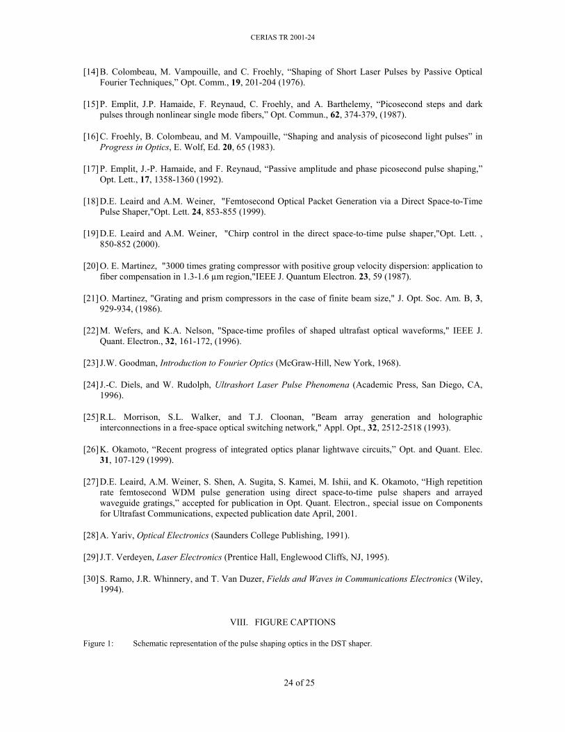
A schematic representation of the pulse shaping components making up the DST pulse shaper is

shown in Fig. 1. A spatially patterned mask is present at the surface of a diffraction grating. A lens

collects and focuses the spatially dispersed frequency components of the input beam that are diffracted

from the grating. At the Fourier plane of the pulse shaping lens, a thin slit filters the dispersed spectrum,

and in the ideal case generates a spatially homogenous output beam whose temporal intensity profile is

given by scaled replica of the spatial masking function present at the diffraction grating. The scaling

parameter between the spatially patterned mask and the output temporal profile will be investigated in this

section.

A. Quantitative Argument The Fourier transform relations used in all the following discussions are listed for completeness:

( ) ( )

( ) ( )

( ) ( )

( ) ( )

1F = dt f t exp[-j t]2

1f t = d F exp[j t]21S k = dx s x exp[jkx]21s x = dk S k exp[-jkx]2

ω ωπ

ω ω ωπ

π

π

∫

∫

∫

∫

(1)

CERIAS TR 2001-24

4 of 25

The key planes to be investigated in the following are shown in Fig. 1. The planes P1 and P2 are

just after transmission through a spatially patterned mask and diffraction off the grating respectively. The

planes P3 and P4 are just prior to and just after the output slit respectively. If the input to the apparatus is

an optical pulse of short duration with a spatial profile given by s(x), then the field just before the

diffraction grating is given by

( ) ( ) ( ) ( )1 in ine x, t s(x) e (t) s x E exp j tdω ω ω= ∝ ∫ (2)

Here s(x) includes both the spatial profile of the input beam, and the effect of transmission through the

spatially patterned mask, ein(t) is the temporal profile of the input field, its Fourier transform, Ein(ω) is the

input spectrum, and x is the transverse spatial coordinate. Assuming a diffraction grating dispersion that is

linear in space and frequency yields the spectrum just after the diffraction grating[21][22]:

( ) ( ) ( ) ( )2 inE x, s x exp -j x Eω β γω ω∝

with the corresponding time domain field given by:

( ) ( ) ( )2 2e x, t E x, exp j tdω ω ω∝ ∫ (3)

The spatial dispersion is written

= c d cos d

λγθ

(4)

where λ is the center wavelength, c is the speed of light, d is the period of the diffraction grating,

and θd is the angle of diffraction. The astigmatism of the diffracting grating is included with the term

coscos

i

d

θβθ

= (5)

with the incident angle given by θi. If the grating-lens, and lens-output slit separations are set equal to the

focal length of the lens, f, then the field just before the output slit is the spatial Fourier transform of eqn. (3)

[23] with the result:

( ) ( )3 in2 xe x, t E ( S - exp j t

fd π γωω ω ω

βλ β

∝ )

∫ (6)

Assuming an ideal thin slit at the apparatus output, and calling the transverse output slit position x = 0 for

convenience yields the field just after the output slit:

CERIAS TR 2001-24

5 of 25

( ) ( )4 ine x, t E ( S - exp j t d γωω ω ωβ

∝ )

∫ (7)

As eqn (7) shows, the output temporal profile is determined by the Fourier transform of the output

spectrum with the result:

( ) ( )4 in-e t e t s tβγ

∝ ∗

(8)

In words then, the output temporal profile is determined by the input field convolved with a scaled

representation of the input spatial profile. The space-to-time conversion constant is given by

i

= c d cos

γ λβ θ

(9)

The spatial profile just before the surface of the diffraction grating is the product of the masking

function with the input beam profile. For a Gaussian beam we can write

( )2

22

-x -j ks x = m(x) exp exp xw 2 R

(10)

The first term, m(x), represents the masking function just prior to the surface of the diffraction

grating. The second term is the Gaussian spatial profile of the input beam, and the final term is a quadratic

phase dependence which arises when the beam is not perfectly collimated at the grating. When eqn. (10)

applies, the output temporal profile is rewritten

( )2 2 2 2

out in 2 2 2

- t - t -j k te t e (t) m exp exp w 2 R

β β βγ γ γ

∗

(11)

Where eout(t) has replaced e4(t) as used in the above discussion in order to emphasis that this is the final

temporal output field. The term inside the {…} is the impulse response function of the DST shaper. It

consists of a scaled version of the mask, multiplied by a Gaussian temporal window function corresponding

to the input Gaussian beam profile as well a quadratic temporal phase variation which arises when the

phase fronts at the grating are not planar. In the remainder of this section we concentrate on the intensity

behavior of the shaped output. In section IV we discuss the chirp corresponding to the quadratic temporal

variation as well as its compensation.

CERIAS TR 2001-24

6 of 25

B. Qualitative Argument

Alternative descriptions of the basic operation of the DST shaper can be obtained by exploring the

fundamental pulse shaping components and configuration shown in Fig. 1. First, the space-to-time

conversion constant can equally be determined by examining the pulse-tilt for a collimated plane wave

diffracted off a grating [24]. The pulse-tilt, or delay across the diffracted beam relative to the input beam

size derived from [24] or a simple trigonometric argument exactly gives the space-to-time conversion

constant (Eqn. 9).

Second, the configuration shown in Fig. 1 will be recognized as a spectrometer arrangement with

the addition of a spatially patterned mask on top of the diffraction grating. If a spectrometer (without a

spatially patterned mask) is configured for maximum spectral resolution (large beam on the diffraction

grating, and thin output slit), the output obviously consists of a narrow spectral feature. If the input consists

of a short temporal duration optical pulse; then, the output pulse, in time, is broadened with respect to the

input due to the spectral filtering performed by the spectrometer, as shown in Fig. 2a. Now if the apparatus

configuration is unperturbed except that the size of the input beam is decreased, as shown in Fig. 2b, the

resolution of the spectrometer is decreased as well. If one considers the input to be a short optical pulse

again; then, the output spectrum is broadened with respect to the previous case, or the temporal duration of

the output is decreased with respect to the previous case. The width of a mask which simply modifies the

spatial extent of the beam on the diffraction grating can then be seen to modify the temporal duration of the

apparatus output directly. This argument illustrates the operation of the DST pulse shaper in a very simple

case and shows its relation to a classical optical spectrometer. In the course of this paper, we will extend

these results to understand the femtosecond response of a generalized spectrometer, allowing generation of

complex optical waveforms, control and compensation of chirp, and the possibility of obtaining multiple

wavelength-shifted versions of a femtosecond pulse sequence simultaneously.

III. DST APPARATUS

A. Complete Apparatus

The schematic representation of the DST pulse shaper shown in Fig. 1 is convenient for

understanding the space-time mapping of the apparatus; however, in practice a slightly more complex

CERIAS TR 2001-24

7 of 25

apparatus provides substantial additional flexibility. The complete DST pulse shaping apparatus is shown

in Fig. 3. The pulse shaping components discussed in the previous section are present to the right of the

dashed line while the mask generation optics are to the left of the dashed line. For the experiments to be

discussed in the following, a Ti:S laser producing 100 fs pulses at a center wavelength of 850 nm is used as

the input to the DST pulse shaper.

The output beam from the source laser is spatially patterned by transmission through a fixed

amplitude mask consisting of a one-dimensional array of transparent rectangles in an otherwise opaque

background. The spatially patterned beam at the ‘pixelation plane’ is imaged by the lens L1, a 100 mm

focal length condensor lens, onto the ‘modulation plane’ through a polarizing beamsplitter cube and

quarter-wave plate. The size (20 µm square) and pitch (62.5 µm center-to-center) of the transparent

elements in the fixed mask as well as the imaging condition of the first lens have been selected to provide

direct compatibility with a high-speed optoelectronic reflection modulator array. This feature is included

so that, in future experiments, individual spatial locations may be set to either a high reflectivity state or a

low state in a programmable fashion. For the work described here, the ‘modulation plane’ consists of a

simple mirror. The spatially patterned beam reflected from the ‘modulation plane’ is imaged, back through

the quarter-wave plate/polarizer combination onto the diffraction grating (1800 lines/mm) by the lens L2, a

75 mm focal length condensor lens. The pulse shaping lens is a 160 mm focal length achromat. The

function of all the mask generation optics is to transfer a one-dimensional spatially patterned intensity

profile from the apparatus input to the diffraction grating. The space-to-time conversion constant, γ/β, is

referenced to the surface at, but before diffracting off, the grating. In order to relate γ/β to the apparatus

input, Eqn. (9) must be multiplied by mag, the overall imaging system magnification of the mask

generation optics. The imaging system magnification is determined by the placement of the spatially

patterned mask, 'modulation plane', and diffraction grating as well as the focal lengths of the two imaging

lenses. In practice, the first imaging operation (from the pixelation mask to the 'modulation plane') is set

for unity magnification while the second imagining operation (from the 'modulation plane' to the grating) is

set for a magnification in the range of 4 to 6.5.

CERIAS TR 2001-24

8 of 25

B. Measuring the Space-to-Time Conversion Constant

A simple measurement of the space-to-time conversion constant, and a first example of pulse

shaping with the DST is shown in Fig. 4. A thin slit replaces the spatially patterned mask at the ‘pixelation

plane’, and intensity cross-correlations are recorded of the output pulses, using a reference pulse directly

from the source laser, for several different transverse positions of the slit at the pixelation plane. The delay

shift between traces gives a measurement of the space-to-time conversion constant including the imaging

system magnification. In the top series of Fig. 4, a 25 µm slit is moved +/-80 µm from the center of the

input beam with an imaging system magnification of 4.2. Measuring the change in delay from one trace to

the next gives a measured space-to-time conversion constant of 29.6 ps/mm. Using the measured

diffraction angle of the grating (54°), the expected space-to-time conversion constant is calculated to be

30.7 ps/mm. A second example of measuring the space-to-time conversion constant is given in Fig. 4b. In

this case, a 20 µm slit is translated in 250 µm increments across the pixelation plane with an imaging

system magnification of 6.5. The measured space-to-time conversion constant is 47.0 ps/mm in excellent

agreement with the calculated value of 47.5 ps/mm. In both the cases shown in Fig. 4, the space-to-time

conversion constant for the pulse shaping components, given by eqn. (9), is held fixed thus demonstrating

the space-time scaling change possible with the geometry of the imaging system.

C. Pulse Train Generation

One target application of the DST pulse shaper is in the generation of trains of pulses, or pulse

sequences, where the state of each pulse in the train, either ‘ON’ or ‘OFF’, is set by the optical transmission

at a specific spatial location. In order to demonstrate the pulse train generation capabilities of the DST

pulse shaper, a periodic fixed mask is inserted at the pixelation plane. Fig. 5 shows the output pulse shapes,

recorded by intensity cross-correlation for two different periodic pixelation patterns and an imaging system

magnification of 4.2. The top trace corresponds to a mask with 20 transparent rectangles 20 µm wide with

62.5 µm center-to-center spacing. This mask generates a train of 20 pulses. The pulse period, 1.88 ps, is in

excellent agreement with the value expected from the space-to-time conversion constant, 7.3 ps/mm, and

imaging system magnification. The bottom trace shows a similar case where every other transparent

feature of the pixelation mask is blocked. As expected, a train of ten pulses with twice the period of the

CERIAS TR 2001-24

9 of 25

previous case is measured at the apparatus output. In both of these cases, the output pulse train is observed

to be superimposed on a roughly Gaussian window. The roll-off in the temporal profile is due to the input

beam profile at the pixelation mask, and the extent of the temporal window is determined from the input

beam profile and the effect of the finite width pulse shaping slit as will be discussed in the following

section. If a uniform pulse train is desired, a diffractive optical element (DOE) could be used instead of the

pixelation mask as a ‘spot-generator’[25].

Fig. 6 shows two final examples of pulse sequence generation with the DST apparatus. In these

cases, individual spatial locations within the 20 element pixelation mask are blocked. The resulting DST

output, again recorded via intensity cross correlation with a short reference pulse directly from the source

laser, is a ‘pulse packet’. These data demonstrate the parallel-to-serial conversion property of the DST

pulse shaper that may play an important role in optical communications. All of the data shown here have

been generated using a fixed pixelation mask to control the spatial pattern present at the diffraction grating.

Equivalently, an optoelectronic modulator array could be used at the ‘modulation plane’ shown in Fig. 3 to

electronically control the transmission of each spatial location. Of course, the excellent ON-OFF contrast

apparent in Figs. 5 and 6 would then be limited by the actual contrast provided by the modulator array.

D. Spectral resolution, temporal window, and efficiency of the DST Pulse Shaper

So far we have assumed a very thin (delta function) slit at the output of the DST apparatus.

Although this provides an ideal pulse shaping response, it is not practical, since the transmitted power

would be zero. In the following we analyze the trade-off between optical efficiency, spectral resolution,

and the pulse shaping temporal window which occurs with a pulse shaping slit of finite width.

First, recall that the field just prior to the output slit is determined by the input spectrum multiplied

by the spatial Fourier transform of the spatial profile at the diffraction grating, Eqn. (6):

( ) ( )3 in2 xe x, t E ( S - exp j t

fd π γωω ω ω

βλ β

∝ )

∫ (6)

We now introduce a general slit with amplitude transmittance o

xa x

, where xo allows the

width of the output slit to be scaled. The field after the slit is now given by

CERIAS TR 2001-24

10 of 25

( ) ( )4 ino

x 2 xe x, t a E ( S - exp j tx f

d π γωω ω ωβλ β

∝ )

∫ (12)

Unlike the case of a delta-function slit, the field is now a now nonseparable function of space and time; the

actual field seen by an experiment depends on where the experiment is placed and any spatial filtering

between the DST output slit and the experiment. In many cases it will be the on-axis field after diffraction

into the far field that will be of interest. This situation is easily treated analytically, since the diffraction

into the far-field is equivalent to a spatial Fourier transform, which should be evaluated at x=0 to obtain the

on-axis field. The result for the far-field on-axis output can be shown to be

( ) ( ) oout in

2 x t-e t e t s t A f

πβγ λ γ

∝ ∗

(13)

where A(k) is the Fourier transform of the slit function. Similarly, the output spectral amplitude is given

by

( ) ( )out ino

- f E E S a2 x

γ ω λ γ ωω ωβ π

∝ ∗

(14)

The terms inside the […] signs of equations (13) and (14) give the impulse response function and spectral

filter function of the DST pulse shaper, respectively. For a sufficiently short input pulse, these give the

pulse shape and the spectral amplitude of the output pulse. In the case of a perfectly collimated input beam

( R = ∞ ), we can rewrite the output field in terms of the masking function and the input Gaussian beam

profile, which gives the following:

( ) ( )2 2

oout in 2 2

2 x t- - te t e t m t exp A w f

πβ βγ γ λ γ

∝ ∗

(15)

and

( ) ( )2 2 2

out in 2o

- - w f E E M exp a4 2 x

γ ω γ ω λ γ ωω ωβ β π

∝ ∗ ∗

(16)

These equations lead to several important observations:

CERIAS TR 2001-24

11 of 25

(1) The impulse response function of a generalized spectrometer (i.e., the DST pulse shaper) is the

inverse Fourier transform of the spectral filter function even for an arbitrary input spatial profile.

(2) The spectral filter function is given by the convolution of appropriately scaled versions of the slit

function and the Fourier transform of the input spatial profile, even for arbitrary input spatial

profiles and slit functions. A similar convolution governs the spectral resolution of an ordinary

spectrometer, where simple input spatial profiles and slit functions are usually considered. In

general, the width of the filter function increases (spectral resolution degrades) as the width of the

slit function (xo) increases.

(3) The impulse response function is given by the product of appropriately scaled versions of the

spatial profile and the Fourier transform of the slit function. Thus, the finite width of the slit leads

to a temporal window function which restricts the temporal range of output waveforms generated

by the DST pulse shaper. The width of the temporal window is inversely proportional to the width

of the slit. For a rectangular slit where a(u) = 1 for |u| < ½ and zero otherwise, the temporal

window function is a sinc with an intensity FWHM

slito

0.886 fT = x

γ λ (17)

In the case of a Gaussian input beam before the mask, the output may also be written as the

product of the scaled masking function times a window function consisting of a Gaussian rolloff

term times the scaled Fourier transform of the slit function.

(3) The effect of the finite slit width is the same as multiplying the input spatial profile by a spatial

windowing function given by o-2 x xA

fπ

λ β

while at the same time setting the width of the slit

to zero.

Fig. 7 shows the calculated temporal window (in terms of the FWHM of the intensity) as a

function of pulse shaping slit width. The space-to-time conversion constant was set to 7.3 ps/mm with

unity imaging system magnification, and the input beam shape was a simple Gaussian beam with radius w

= 1.0 mm just before the grating. For slit widths below approximately 30 microns, the temporal window is

CERIAS TR 2001-24

12 of 25

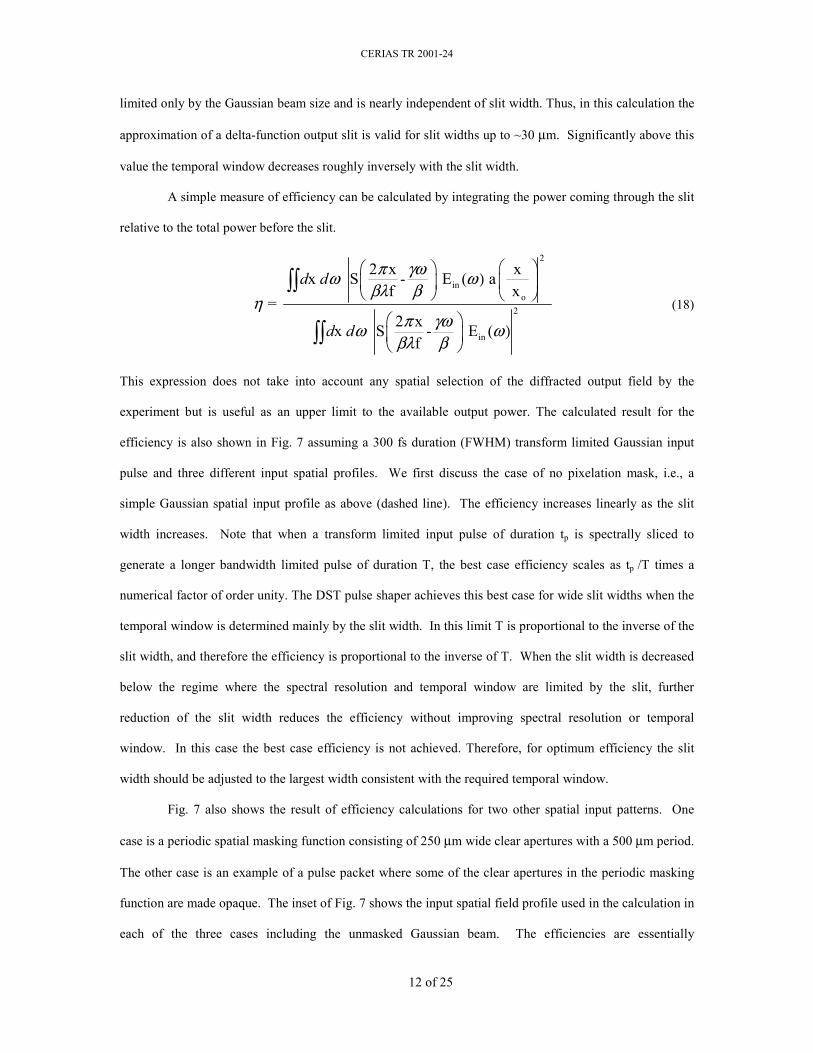
limited only by the Gaussian beam size and is nearly independent of slit width. Thus, in this calculation the

approximation of a delta-function output slit is valid for slit widths up to ~30 µm. Significantly above this

value the temporal window decreases roughly inversely with the slit width.

A simple measure of efficiency can be calculated by integrating the power coming through the slit

relative to the total power before the slit.

2

ino

2

in

2 x xx S - E ( a f x

= 2 xx S - E (

f

d d

d d

π γωω ωβλ β

ηπ γωω ω

βλ β

)

)

∫∫

∫∫ (18)

This expression does not take into account any spatial selection of the diffracted output field by the

experiment but is useful as an upper limit to the available output power. The calculated result for the

efficiency is also shown in Fig. 7 assuming a 300 fs duration (FWHM) transform limited Gaussian input

pulse and three different input spatial profiles. We first discuss the case of no pixelation mask, i.e., a

simple Gaussian spatial input profile as above (dashed line). The efficiency increases linearly as the slit

width increases. Note that when a transform limited input pulse of duration tp is spectrally sliced to

generate a longer bandwidth limited pulse of duration T, the best case efficiency scales as tp /T times a

numerical factor of order unity. The DST pulse shaper achieves this best case for wide slit widths when the

temporal window is determined mainly by the slit width. In this limit T is proportional to the inverse of the

slit width, and therefore the efficiency is proportional to the inverse of T. When the slit width is decreased

below the regime where the spectral resolution and temporal window are limited by the slit, further

reduction of the slit width reduces the efficiency without improving spectral resolution or temporal

window. In this case the best case efficiency is not achieved. Therefore, for optimum efficiency the slit

width should be adjusted to the largest width consistent with the required temporal window.

Fig. 7 also shows the result of efficiency calculations for two other spatial input patterns. One

case is a periodic spatial masking function consisting of 250 µm wide clear apertures with a 500 µm period.

The other case is an example of a pulse packet where some of the clear apertures in the periodic masking

function are made opaque. The inset of Fig. 7 shows the input spatial field profile used in the calculation in

each of the three cases including the unmasked Gaussian beam. The efficiencies are essentially

CERIAS TR 2001-24

13 of 25

indistinguishable for the two masked cases (dash-dot lines), which are also very close but slightly below the

efficiency in the unmasked case. The integrated intensity in the input masked spatial profile is held

constant in each case as would be the case if a DOE is used to spatially pattern the input beam without loss

If loss is incurred in shaping the input spatial profile, e.g. by using an amplitude mask, this reduces the

overall system efficiency to a level below that predicted by eqn. (18). Notice that, for a fixed input pulse

and temporal window, the efficiency is roughly independent of the masking function. This behavior was

previously predicted in [18].

We can gain further insight into these trends when the following two conditions hold:

(1) The slit function, o

xa x

, is much narrower then the finest features in 2 xS

fπ

βλ

. This is the

narrow slit limit, in which the temporal window is limited by the input beam size rather then by

the slit. This is the most interesting regime for the DST pulse shaper.

(2) S - γωβ

is much narrower than Ein(ω). This means that the input pulse is much narrower then

the narrowest temporal features in the scaled spatial profile - ts β

γ

.

With these assumptions eqn. (18) for the efficiency simplifies to

2

o2

in

in

2 x x a f x

E ( E (0

d

d

πγλ

ηωω

≈

))

∫

∫ (19)

In this limit, which corresponds to slit widths below ~30 µm in Figure 7, the efficiency is independent of

the masking function. This expression can be further simplified if, for example, we assume a rectangular

slit of width xo and a Gaussian input pulse of the form ( )2

in 2p

- e expttt

∼ . The efficiency becomes

o p2 x t

fπ

ηγ λ

≈ (20)

CERIAS TR 2001-24

14 of 25

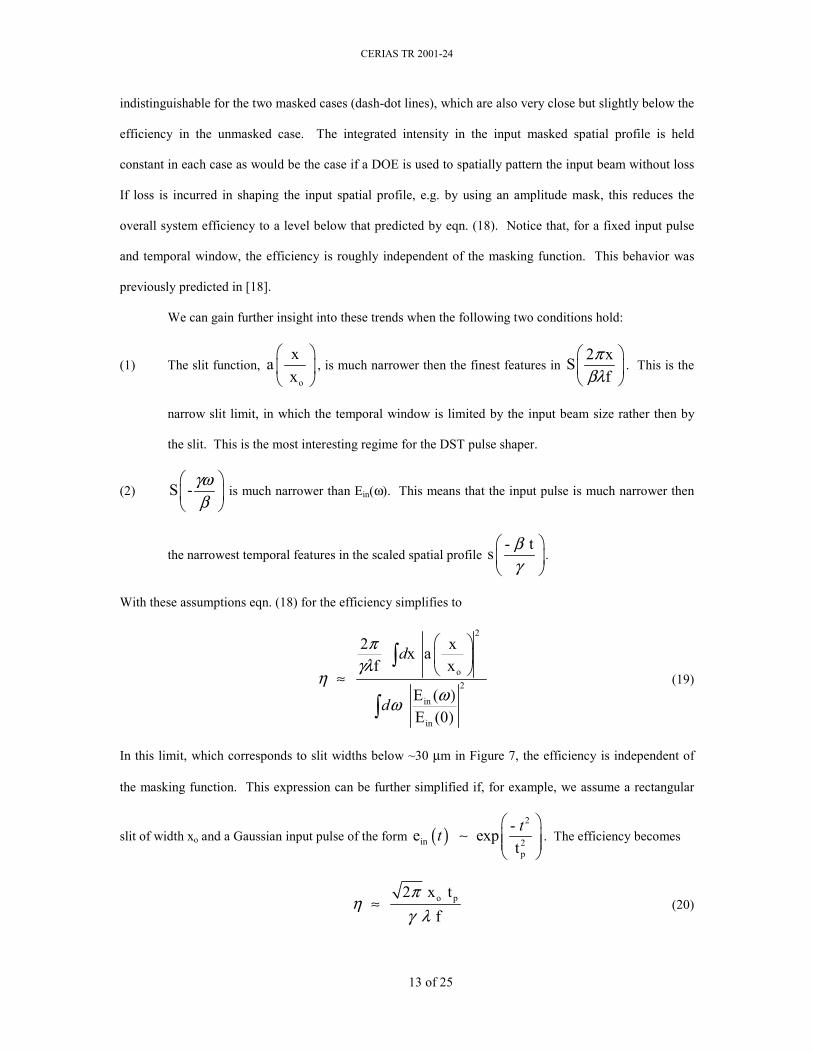
The efficiency increases linearly with slit width, provided that assumption (1) remains valid. The best

efficiency possible for a given temporal window T can be estimated by increasing xo until the temporal

window due to the slit decreases to T. Using eqn. (17) to replace xo in terms of T, one obtains

pt 2.2

Tη ≈ (21)

This expression should be taken as approximate, since assumption (1) is beginning to be violated.

Nevertheless, this result is consistent with our discussion above and indicates that the best case efficiency

scales as the ratio of the input pulse width to the temporal window, independent of the detailed shape of the

output waveform. Equations (19)-(21) explain all the key features of the efficiency curves observed in the

numerical results for the narrow-slit regime (xo < ~30 µm). It is interesting to note that the same behavior

continues to hold in the cases examined even in the wide-slit regime (xo > ~30 µm) for which the

assumptions made above do not hold.

Finally, we note that instead of considering a slit function as above, it is also possible to replace

the output slit with a waveguide. This case is relevant to integrated spectrometer devices such as arrayed

waveguide grating demultiplexors [26] used in WDM communications. When the output slit is replaced by

a single-mode waveguide, a spatially uniform output field is produced automatically with no further spatial

filtering. The temporal window and efficiency can be computed exactly by calculating the overlap integral

of the field with the waveguide on a frequency by frequency basis. Although the details are not given here,

we note that important features discussed above, such as the Fourier transform relationship between the

spectral filter function and the temporal impulse response function, remain valid. A complete description

of the analogy between the bulk optics DST pulse shaper and the integrated-optic arrayed waveguide

grating, used for the generation of very-high repetition rate pulse train bursts, is contained in [27].

IV. CHIRP IN THE DST APPARATUS

A. Effect of input phase curvature

The imaging operations shown in Fig. 3 have one side effect that has thus far not been discussed:

in addition to relaying the desired intensity profile of the pixelated input beam onto the diffraction grating,

the imaging operation places a quadratic spatial phase variation on the grating as well. The space-to-time

CERIAS TR 2001-24

15 of 25

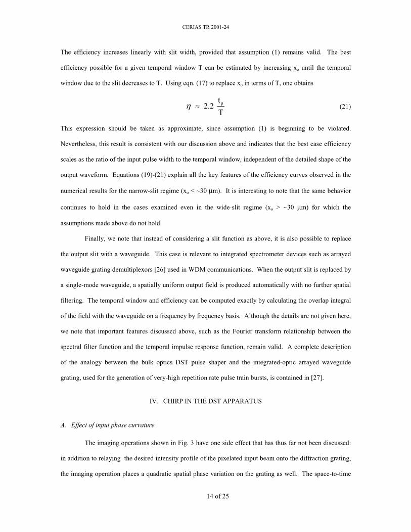
conversion property of the DST operates on this spatial phase variation as well as on the intensity profile.

The quadratic spatial phase is transformed into a quadratic temporal phase on the output waveform, and

hence a chirp.

The magnitude and sign of the chirp attributable to the apparatus itself can be calculated if we

assume a very short input pulse and assume m(x)=1, i.e., there is no pixelation mask. Then eqn. (11) can

be simplified to

( )2 2 2 2

out 2 2 2

- t -j k te t exp exp w 2 R

β βγ γ

(22)

This is of the form

( ) 2e t exp - t ∝ Γ (23)

where the carrier term, exp(jωot) is implied, and Γ has both real and imaginary parts.

r i= + j Γ Γ Γ (24)

with 2

2 2r wβ

γΓ = and

2

22ikRβγ

Γ = . The instantaneous frequency is given by the time derivative of the

total phase:

( ) ( )2totalinst o it = = t - t

t tφω ω∂ ∂ Γ∂ ∂

(25)

and the chirp, sometimes called a frequency modulation, is given by the time derivative of the

instantaneous frequency:

insti = -2

tω∂ Γ∂

(26)

Finally, it is convenient to express the chirp in terms of wavelength instead of frequency with the

result

2 2

i2

= = t c c R λ λ λ β

π γ∂ Γ∂

(27)

Expressed in terms of the fundamental parameters of the DST pulse shaper, the chirp is given by

2 2

ic d cos = t R λ θ

λ∂∂

(28)

CERIAS TR 2001-24

16 of 25

With this result it is possible to estimate the chirp expected to be present on the output of the DST

pulse shaper.

B. Chirp Measurement

In order to measure the chirp on the output of the DST pulse shaper, the pixelation mask is

replaced by a single slit. As in Fig. 4, a single output pulse is generated from the DST shaper with this

pixelation mask. The width of the pixelation mask is chosen as a trade-off between the output pulse width,

and the width of the power spectrum at the apparatus output. Fig. 8 shows results of our chirp

measurement. The pixelation mask is translated across the input beam, and intensity cross correlations and

power spectra are recorded as a function of pixelation mask position. The center wavelengths of the

measured power spectra are plotted as a function of the time delays corresponding to each of the transverse

pixelation mask positions. The slopes of the two curves in Fig. 8 are measures of the DST chirps for

different imaging system magnifications. The slopes are 6.4 ps/nm and 6.8 ps/nm for imaging system

magnifications of 4.2 and 6.5 respectively.

A theoretical estimate of the expected chirp on the DST output can be obtained by numerically

propagating a beam through the imaging system optics using Gaussian beam methods (ABCD matrices)

[28][29] in order to determine an expected phase front curvature at the surface of the diffraction grating.

Assuming a flat phase front at the surface of the pixelation mask, estimated values of chirp are 7.2 ps/nm

and 8.5 ps/nm for imaging system magnifications of 4.2 and 6.5 respectively, which are in reasonable

agreement with the experimental values. The difference between the measured and calculated chirps is due

to the fact that the phase front is not completely flat at the pixelation mask.

C. Diffraction Analysis: Chirp compensation by the DST apparatus

If the DST apparatus is to be used in optical communications applications, it will usually be

necessary to control the chirp, and possibly set it to zero. One way to eliminate the chirp in the DST

apparatus would be to utilize a telescopic configuration for relaying the masked spatial profile from the

apparatus input to the diffraction grating. However, a flat phase front would be present at the diffraction

grating only if a perfectly collimated (or focused) beam were present at the apparatus input with a precisely

CERIAS TR 2001-24

17 of 25

positioned telescopic configuration. Since these strict requirements may be undesirable in some cases, it is

useful to explore alternative methods for eliminating the final term of Eqn. (22).

To this end we have performed a diffraction analysis of the DST apparatus [19]. Similar analyses

have been previously performed for pulse stretchers [21] and pulse shapers [22]. In [19] we showed that

changing the pulse shaping lens – output slit separation introduces a quadratic temporal phase term (chirp)

to the output field that can be used to cancel the chirp resulting from the phase front curvature present at the

diffraction grating. In the following, we generalize the diffraction analysis in order to permit both the

grating-lens and lens-slit separations to vary.

Fig. 9 shows a schematic representation of the different propagation regions included in the

diffraction analysis. The grating-lens and lens-slit separations are denoted d1 and d2 respectively.

Following a procedure similar to [21] and [22], and starting with Eqn. (3), the spectral amplitude of the

field just prior to the diffraction grating is written

( ) ( ) [ ] ( )2 inE x, s x exp -j x Eω β γ ω ω∝ (29)

The field just after the grating is propagated in the Fresnel regime to just before the pulse shaping

lens [23], giving the following new expression for the spectral amplitude:

( ) ( ) 23 2 2 2 2 2

1 1-

j k -j kE x, x E x , exp x exp x x2 d d

dω ω∞

∞

∝

∫ (30)

Then the effect of the lens is included:

( ) ( ) 24 3

-j kE x, E x, exp x2 f

ω ω = (31)

followed by another propagation in the Fresnel regime to the output slit:

( ) ( ) 25 4 4 4 4 4

2 2-

j k -j kE x, x E x , exp x exp x x2 d d

dω ω∞

∞

∝

∫ (32)

Finally the effect of a delta-function output slit is included:

( ) ( ) ( )6 5E x, E x, xω ω δ= (33)

In order to relate the input and output fields, equations (29)-(33) are combined with Eqn. (10) for

s(x) and the identity [30]

CERIAS TR 2001-24

18 of 25

( )2

2 j -j exp j x + x = exp4

dx π ξα ξα α

∞

−∞

∫ (34)

After considerable manipulation, we obtain the result

( ) ( ){ }out ine (t) e (t) t exp -j tφ∝ ∗ Ν (35)

where

( )2 2

2 2

- t - tt = m expw

β βγ γ

Ν

(36)

determines the temporal intensity profile of the output, and

( )2

222

1 2 1 2

k d - ft = - t2 R d f d f - d d

βφγ

+

(37)

gives the quadratic temporal phase and hence the chirp. The output chirp can be manipulated (in a special

case compensated or set to zero) by varying d1 and d2. The intensity profile and space-to-time conversion

constant are expected to remain invariant as the chirp is manipulated in this way.

Unlike the well known grating and lens pulse stretcher [21], the chirp is most strongly affected by

the lens-slit separation (d2). When d2 is fixed at the focal length of the lens (d2 = f), output chirp is

independent of the diffraction grating – lens separation, d1. Further, for bandwidth limited input pulses, the

measured chirp in the d2 = f case can provide a measure of the phase front curvature at the surface of the

diffraction grating, R. After determining the value of R in this way, the chirp can be calculated as a

function of d1 and d2 with no further adjustable parameters using Eqn. (27) with Γi replaced by

2

2i 2

1 2 1 2

k d - f = - 2 R d f d f - d d

βγ

Γ +

(38)

The output chirp can be set to zero by adjusting d1 and d2 to achieve 0iΓ = (again assuming

unchirped input pulses). It is interesting to note that in the case of a converging or diverging input beam at

the grating (i.e., R ≠ ∞ ), the beam is brought to a focus at a position other than the back focal plane of the

lens. By using ABCD matrices, one can easily show that for d1 and d2 yielding 0iΓ = , an input Gaussian

CERIAS TR 2001-24

19 of 25

beam with phase front radius of curvature R is brought to focus at exactly the position of the pulse shaping

slit.

D. Chirp Compensation Experimental Verification

In order to verify the predictions made in the previous section, we have performed a series of chirp

measurements as outlined in section IV(B). The predicted and measured chirp are compared, with the

value of R determined from the measured chirp in the configuration d1 = d2 = f.

Fig. 10 shows the measured chirp, in nm/ps, and space-to-time conversion constant as a function

of the deviation of the pulse shaping lens-slit separation, d2, away from the focal length of the pulse

shaping lens. This data was recorded for the configuration where the diffraction grating-pulse shaping lens

separation was fixed at the focal length of the lens (d1 = f). The predicted and measured chirp are in

excellent agreement over a large range of lens-slit separations. A chirp-free output is achieved for d2

approximately 119 mm beyond the back focal plane of the lens. Further, the space-to-time conversion

constant is observed to be flat as the chirp is varied over a wide range. This provides a first indication that

the output intensity profile is invariant as the chirp is varied.

Fig. 11 shows the measured chirp in two special cases. In one case, the diffraction grating-pulse

shaping lens separation, d1, is allowed to vary while the pulse shaping lens – output slit separation, d2, is

fixed at the focal length of the lens, f. In the second case the converse is true, d2 is varied while d1 = f is

maintained. In the first case, the output chirp does not change with d1 as expected from our prediction.

The second case is data similar to that shown in Fig. 10, and is repeated just for reference.

Two specific implementations of the general case (neither d1 nor d2 equal to f) are shown in Fig.

12, along with the special case of d1 = f. In the top trace, the grating-lens separation is set to a fixed value

of 110 mm (compared to f = 160 mm), and the predicted chirp is plotted as a function of the lens-slit

separation, d2. In the bottom case, both d1 and d2 are varied, but their sum is held fixed at twice the focal

length of the lens. Both of these new cases are tested by a chirp measurement at d2 = 60 mm. In each case

the calculated and measured chirp are in excellent agreement.

Finally, in order to verify that the output intensity profile is invariant as the chirp is adjusted,

intensity cross correlation traces of an ultrafast data packet were recorded for three different amounts of

CERIAS TR 2001-24

20 of 25

output chirp. The results are shown in Fig. 13, and in all cases d1 = f. The top trace was taken in a

moderately chirped configuration when d2 = f. The middle trace was taken in a partially compensated chirp

configuration, d2-f = 66 mm, and the bottom trace was taken in a chirp-free configuration, d2-f = 119 mm.

The general shape of each of the three cross correlation traces is the same verifying that the output intensity

profile is unchanged as the chirp on the DST output is varied. The minor differences in the envelopes of

the three traces is due to slight changes in the centering of the pixelation mask on the input beam from one

measurement to the next.

V. MULTIPLE OUTPUT CHANNELS FROM THE DST PULSE SHAPER

In all the discussions thus far, a single output slit has been assumed, with the implication is that

this slit is centered on the dispersed frequency spectrum. Specifically, the ideal output slit was taken to be

positioned at an arbitrary, but convenient position, x = 0. As we shall see any other transverse position of

the output slit yields exactly the same intensity profile as Eqn. (8), but with a wavelength shift. In fact, a

multiple element slit could be used instead of the single slit resulting in multiple spatially separated output

beams. This section will focus on the output multiple wavelength nature of the DST apparatus.

A. Mathematical Description

The multiple output nature of the DST apparatus follows directly from the previous discussions of

the space-time mapping. In the following, for convenience, the DST apparatus is assumed to be configured

chirp-free. That is, the pulse shaping lens – output slit separation, d2, is set to cancel the quadratic temporal

phase term due to the phase front radius of curvature at the diffraction grating. However, the important

features derived below also hold for the more general case where the chirp is not compensated. In the

chirp-free case, the spatial profile mapped to the time domain consists of just the first two terms of Eqn.

(10) – the masking function, and the beam profile:

( )2

2

-xs x = m(x) expw

(39)

The complex spectrum just prior to the output slit(s) is given by:

( )3 in2 xE x, S - E (

fπ γωω ω

βλ β

∝ )

(40)

CERIAS TR 2001-24

21 of 25

Consider now a thin slit at lateral position xs, i.e., of the form δ(x-xs). The filtered spectrum now

has the form

( ) ( )4 in s2 xE x, S - E ( x - x

fπ γωω ω δ

βλ β

∝ )

(41)

Note that S(…) is the spectral response function of the generalized spectrometer. Eqn. (41) shows

that a transverse movement of the output slit leads to a simple shift in the spectral response function of the

DST pulse shaper, just as it would in an ordinary spectrometer, even though the spectral response of the

DST may be much more complex than that of a spectrometer.

The time domain response corresponding to Eqn. (41) is given by

( ) ( ) sout in

j 2 x- te t e t s exp tf

πβγ γλ

∝ ∗

(42)

The impulse response function is given by the terms inside the {…} sign and consists of two

terms. The first, s(-βt/γ), represents the space-to-time conversion constant and is unchanged compared to

our earlier treatment. The second, linear phase term represents a frequency shift. Thus, a lateral movement

of the output slit tunes the output optical frequency while leaving the intensity profile of the shaped output

waveform unaffected.

We can also consider a multiple output slit element which spatially separates each output beam in

a non-overlapping manner. The output from each independent slit is still given by equations (41) and (42),

with the appropriate slit position inserted for xs. Thus, the DST pulse shaper should be able to

simultaneously generate multiple spatially separated, wavelength shifted outputs, each with the identical

intensity profile. In cases where such multiple outputs are useful, this increases the overall optical

efficiency by a factor equal to the number of outputs.

B. Measurements

In order to demonstrate the shift in output center wavelength as a function of transverse output slit

position, a periodic pixelation mask consisting of 20 transparent rectangles in an otherwise opaque

background was inserted into the pixelation plane of the DST pulse shaper. As shown previously, use of

this pixelation mask will result in a temporal output intensity profile that is a train of pulses. Accordingly,

CERIAS TR 2001-24

22 of 25

one expects this output temporal profile to correspond to a periodically modulated power spectrum after the

output slit. Fig. 14 shows a series of nine power spectra recorded at periodic transverse output slit positions

separated by 1 mm. The trend of a shift in center wavelength as a function of transverse output slit position

is quite evident when plotted in this manner. Further, Fig. 14 shows that multiple spatially separated output

channels could be generated by replacing the single output slit used in these measurements with a multiple

element slit.

The invariant shape of the output power spectra in Fig. 14 imply that the temporal profile of each

output is invariant as well. Further evidence of this assertion is shown in Fig. 15. Here, intensity cross

correlation traces are shown for two different output slit positions separated by 2 mm transverse distance as

well as two different pixelation mask patterns. The 2 mm transverse distance between the output slit

positions corresponds to a 3.6 nm shift in the center wavelength of the output power spectra. The left two

traces correspond to the pixelation mask used to measure the power spectra shown in Fig. 14 – a periodic

20 pixel ‘pulse train’ mask. The right two traces correspond to a ‘data packet’ mask similar to the mask

used for the data presented in Fig. 6. These four cross correlation’s clearly shown the invariant nature of

the output temporal intensity profile as expected from Eqn. (42) and the recorded power spectra.

VI. CONCLUSION

The DST pulse shaper has been explored both theoretically and experimentally. The space-time

scaling is related to the dispersion and astigmatism of the diffraction grating used in the pulse shaper. The

direct scaling between input spatial profile and output temporal intensity profile may prove advantageous

for applications in optical communications or photonic A/D conversion. The output chirp of the apparatus,

of particular importance for high bit-rate optical communications systems, may be controlled/compensated

by a simple geometrical change in the component placement of the apparatus without altering the output

temporal intensity profile. Also, multiple spatially separated output channels may be generated

simultaneously by utilizing a multiple slit element at the apparatus output. This feature of the DST

apparatus could be of benefit to WDM optical communications, or the generation of multiple,

synchronized, but wavelength shifted pulse trains for high-rate sampling in photonic A/D.

CERIAS TR 2001-24

23 of 25

This material is based upon work supported by, or in part by the U.S. Army Research Office under

contract DAAG55-98-1-0514, and by sponsors of the Center for Education and Research in Information

Assurance and Security.

VII. REFERENCES

[1] A. M. Weiner, J. P. Heritage, and E. M. Kirschner, "High-resolution femtosecond pulse shaping,"J. Opt. Soc. Amer. B 5, 1563-1572 (1988).

[2] A. M. Weiner, D. E. Leaird, J.S. Patel, and J.R. Wullert, "Programmable shaping of femtosecond pulses by use of a 128-element liquid-crystal phase modulator,"IEEE J. Quantum Electron. 28, 908-920 (1992).

[3] A.M. Weiner, "Femtosecond optical pulse shaping and processing,"Prog. Quantum Electron. 19 (3), 161-238 (1995).

[4] A.M. Weiner, "Femtosecond pulse shaping using spatial light modulators,"Rev. Sci. Instr. 71, 1929-1960 (2000).

[5] M.M. Wefers and K.A. Nelson, "Generation of high-fidelity programmable ultrafast optical waveforms,"Opt. Lett. 20, 1047-1049 (1995).

[6] M.A. Dugan, J.X. Tull, and W.S. Warren, "High resolution acousto-optic shaping of unamplified and amplified femtosecond laser pulses,"J. Opt. Soc. Am. B 14 (9), 2348-2358 (1997).

[7] D. Yelin, D. Meshulach, and Y. Silberberg, "Adaptive femtosecond pulse compression,"Optics Letters 22 (23), 1793-1795 (1997).

[8] A. Assion, T. Baumert, M. Bergt, T. Brixner, B. Kiefer, V. Seyfried, M. Strehle, and G. Gerber, "Control of Chemical Reactions by Feedback-Optimized Phase-Shaped Femtosecond Laser Pulses,"Science 282, 919-922 (1998).

[9] Christopher J. Bardeen, Vladislav V. Yakovlev, Kent R. Wilson, Scott D. Carpenter, Peter M. Weber, and Warren S. Warren, "Feedback quantum control of molecular electronic population transfer,"Chemical Physics Letters 280, 151-158 (1997).

[10] S. Shen and A.M. Weiner, "Complete dispersion compensation for 400-fs pulse transmission over 10-km fiber link using dispersion compensating fiber and spectral phase equalizer,"IEEE Phot. Tech. Lett. 11, 827-829 (1999).

[11] H.P. Sardesai, C-.C Chang, and A.M.Weiner, "A Femtosecond Code-Division Multiple-Access Communication System Testbed,"Journal of Lightwave Technology 16, 1953-1964 (1998).

[12] T. Kurokawa, H. Tsuda, K. Okamoto, K. Naganuma, H. Takenouchi, Y. Inoue, and M. Ishii, "Time-space conversion optical signal processing using arrayed waveguide grating,"Electron. Lett. 33, 1890-1891 (1997).

[13] H. Tsuda, K.Okamoto, T. Ishii, K. Naganuma, Y. Inoue, H. Takenouchi, and T. Kurokawa, "Second- and third-order dispersion compensator using a high-resolution arrayed-waveguide grating,"IEEE Phot. Tech. Lett. 11, 569-571 (1999).

CERIAS TR 2001-24

24 of 25

[14] B. Colombeau, M. Vampouille, and C. Froehly, “Shaping of Short Laser Pulses by Passive Optical Fourier Techniques,” Opt. Comm., 19, 201-204 (1976).

[15] P. Emplit, J.P. Hamaide, F. Reynaud, C. Froehly, and A. Barthelemy, “Picosecond steps and dark pulses through nonlinear single mode fibers,” Opt. Commun., 62, 374-379, (1987).

[16] C. Froehly, B. Colombeau, and M. Vampouille, “Shaping and analysis of picosecond light pulses” in Progress in Optics, E. Wolf, Ed. 20, 65 (1983).

[17] P. Emplit, J.-P. Hamaide, and F. Reynaud, “Passive amplitude and phase picosecond pulse shaping,” Opt. Lett., 17, 1358-1360 (1992).

[18] D.E. Leaird and A.M. Weiner, "Femtosecond Optical Packet Generation via a Direct Space-to-Time Pulse Shaper,"Opt. Lett. 24, 853-855 (1999).

[19] D.E. Leaird and A.M. Weiner, "Chirp control in the direct space-to-time pulse shaper,"Opt. Lett. , 850-852 (2000).

[20] O. E. Martinez, "3000 times grating compressor with positive group velocity dispersion: application to fiber compensation in 1.3-1.6 µm region,"IEEE J. Quantum Electron. 23, 59 (1987).

[21] O. Martinez, "Grating and prism compressors in the case of finite beam size," J. Opt. Soc. Am. B, 3, 929-934, (1986).

[22] M. Wefers, and K.A. Nelson, "Space-time profiles of shaped ultrafast optical waveforms," IEEE J. Quant. Electron., 32, 161-172, (1996).

[23] J.W. Goodman, Introduction to Fourier Optics (McGraw-Hill, New York, 1968).

[24] J.-C. Diels, and W. Rudolph, Ultrashort Laser Pulse Phenomena (Academic Press, San Diego, CA, 1996).

[25] R.L. Morrison, S.L. Walker, and T.J. Cloonan, "Beam array generation and holographic interconnections in a free-space optical switching network," Appl. Opt., 32, 2512-2518 (1993).

[26] K. Okamoto, “Recent progress of integrated optics planar lightwave circuits,” Opt. and Quant. Elec. 31, 107-129 (1999).

[27] D.E. Leaird, A.M. Weiner, S. Shen, A. Sugita, S. Kamei, M. Ishii, and K. Okamoto, “High repetition rate femtosecond WDM pulse generation using direct space-to-time pulse shapers and arrayed waveguide gratings,” accepted for publication in Opt. Quant. Electron., special issue on Components for Ultrafast Communications, expected publication date April, 2001.

[28] A. Yariv, Optical Electronics (Saunders College Publishing, 1991).

[29] J.T. Verdeyen, Laser Electronics (Prentice Hall, Englewood Cliffs, NJ, 1995).

[30] S. Ramo, J.R. Whinnery, and T. Van Duzer, Fields and Waves in Communications Electronics (Wiley, 1994).

VIII. FIGURE CAPTIONS

Figure 1: Schematic representation of the pulse shaping optics in the DST shaper.

CERIAS TR 2001-24

25 of 25

Figure 2: Spectrometer analogy for the space-time scaling of the DST shaper.

Figure 3: Complete DST apparatus.

Figure 4: Measurement of the space-to-time conversion constant for imaging system magnifications of (A) 4.2 and (B) 6.5.

Figure 5: Pulse train generation using a periodic pixelation mask.

Figure 6: Optical 'data packet' generation from the DST shaper.

Figure 7: Temporal window (solid) and efficiency (dash and dot-dash) as a function of pulse shaping slit width. The inset shows the spatial field profile present at the diffraction grating for the efficiency calculations. The dashed line is for a Gaussian profile while the result for both patterned spatial profiles is indicated by the dash-dot line.

Figure 8: Measurement of apparatus chirp for two imaging system magnifications.

Figure 9: Diffraction analysis planes of interest.

Figure 10: Chirp and space-to-time conversion constant measured as the pulse shaping lens – slit separation is varied.

Figure 11: Chirp in two special cases. Solid: fix grating-pulse shaping lens separation and vary lens slit. Dash: fix lens-pulse shaping slit while varying grating-lens separation.

Figure 12: Measurement of chirp in the general case.

Figure 13: Output intensity profiles measured by cross correlation with an unshaped reference pulse for pulse shaping lens-slit separations of 160 mm, 226 mm, and 279 mm.

Figure 14: Output power spectra as a function of transverse pulse shaping slit position.

Figure 15: Output intensity profiles for pulse shaping slit positions separated by 2mm and two different pixelation masks.

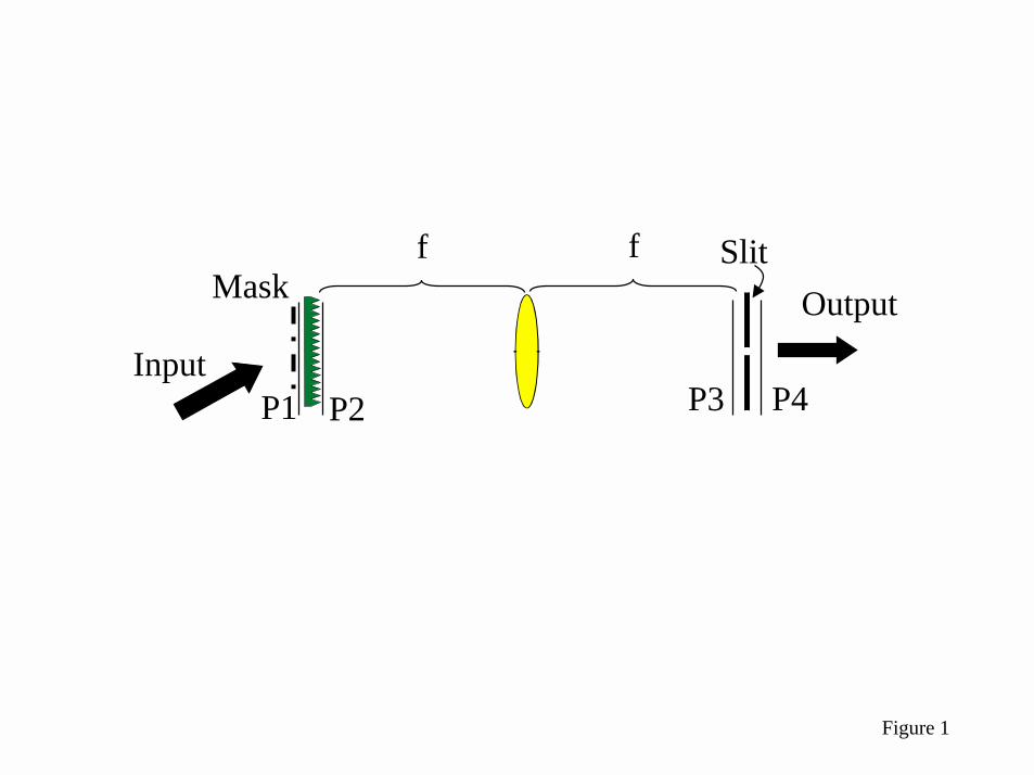
Figure 1

MaskSlit

P1 P3 P4

Output

f f

InputP2

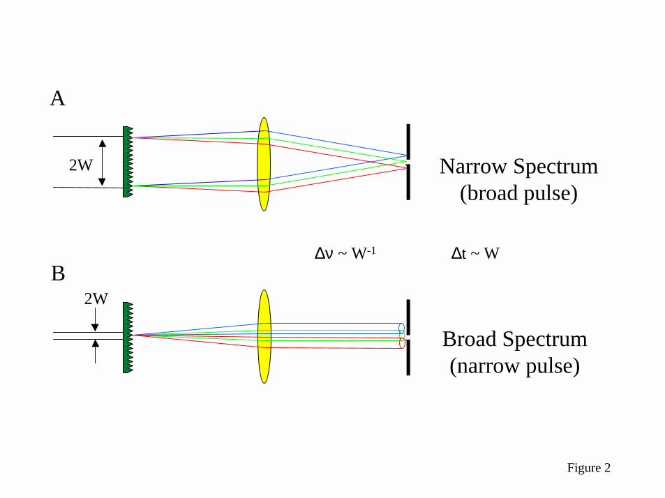
Figure 2

Narrow Spectrum(broad pulse)

Broad Spectrum(narrow pulse)

2W

2W

∆ν ~ W-1 ∆t ~ W

A

B

Figure 3

Pixelation Plane(fixed mask)

Inputλ/4

‘Modulation’ Plane

Slit

PulseShaping

MaskGeneration

f

L1

L2

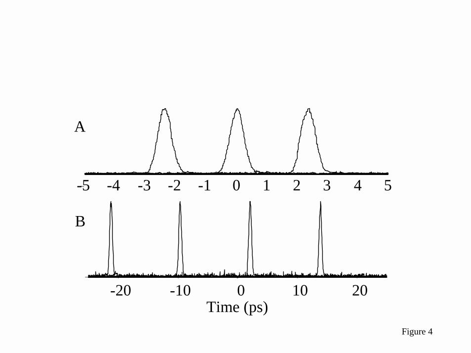
Figure 4

-5 -4 -3 -2 -1 0 1 2 3 4 5

Time (ps)-20 -10 0 10 20

A

B

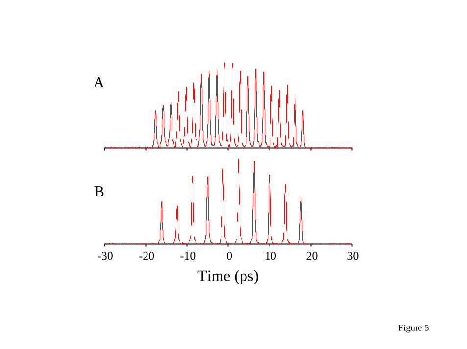
Figure 5

Time (ps)-30 -20 -10 0 10 20 30

A

B

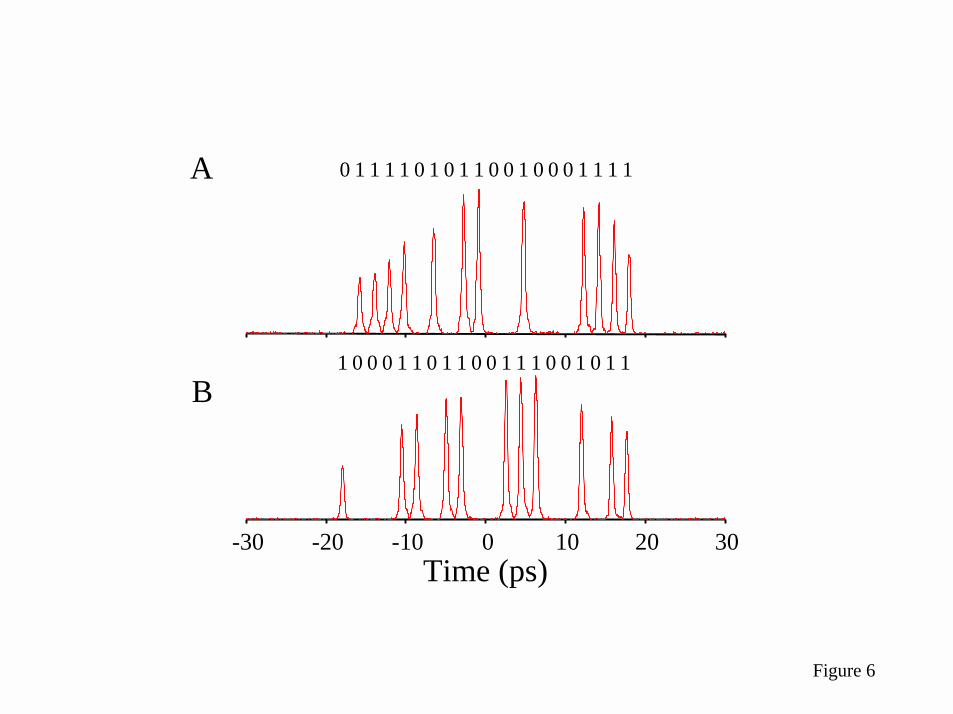
Figure 6

Time (ps)-30 -20 -10 0 10 20 30

1 1 1 1 0 1 10 1 0 0 1 0 0 0 1 1 1 10

0 0 0 1 1 0 11 0 0 1 1 1 0 0 1 0 1 11

A

B

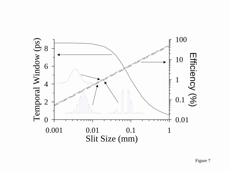
Figure 7

Slit Size (mm)0.001 0.01 0.1 1

Tem

pora

l Win

dow

(ps)

0

2

4

6

8 Efficiency (%)

0.01

0.1

1

10

100

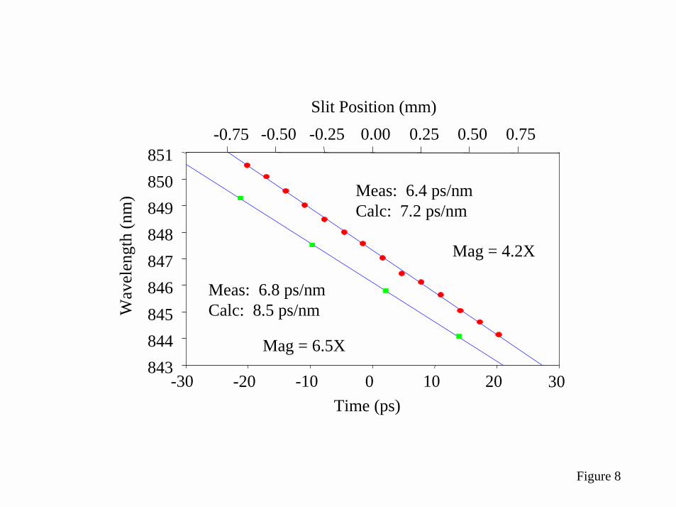
Figure 8

Meas: 6.4 ps/nmCalc: 7.2 ps/nm

Time (ps)-30 -20 -10 0 10 20 30

Wav

elen

gth

(nm

)

843844845846847848849850851

Slit Position (mm)-0.75 -0.50 -0.25 0.00 0.25 0.50 0.75

Meas: 6.8 ps/nmCalc: 8.5 ps/nm

Mag = 4.2X

Mag = 6.5X

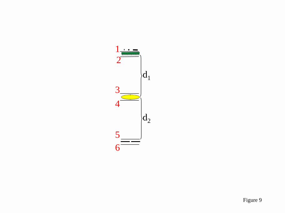
Figure 9

d1

d2

2

34

56

1

Figure 10

d2 - f (mm)0 25 50 75 100 125 150 175

Chi

rp (n

m/p

s)

-0.10

-0.05

0.00

0.05

0.10

0.15

0.20Space-to-Tim

eC

onversion Constant (ps/m

m)

36

38

40

42

44

Chirp = 0

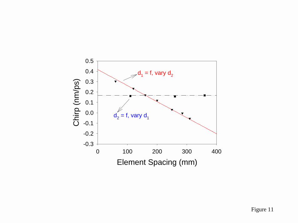
Figure 11

Element Spacing (mm)0 100 200 300 400

Chi

rp (n

m/p

s)

-0.3

-0.2

-0.1

0.0

0.1

0.2

0.3

0.4

0.5

d1 = f, vary d2

d2 = f, vary d1

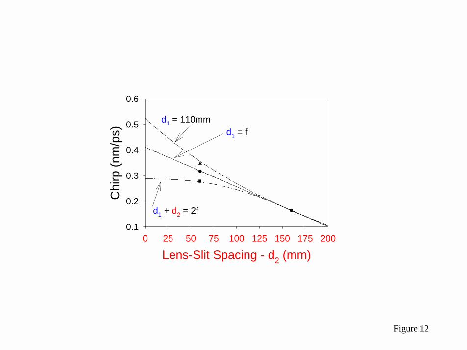
Figure 12

Lens-Slit Spacing - d2 (mm)0 25 50 75 100 125 150 175 200

Chi

rp (n

m/p

s)

0.1

0.2

0.3

0.4

0.5

0.6

d1 = fd1 = 110mm

d1 + d2 = 2f

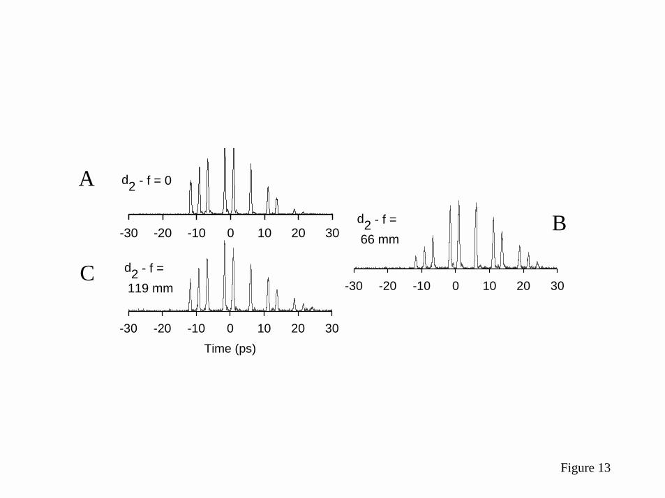
Figure 13

-30 -20 -10 0 10 20 30

d2 - f = 66 mm-30 -20 -10 0 10 20 30

d2 - f = 0

Time (ps)-30 -20 -10 0 10 20 30

d2 - f = 119 mm

A

C

B

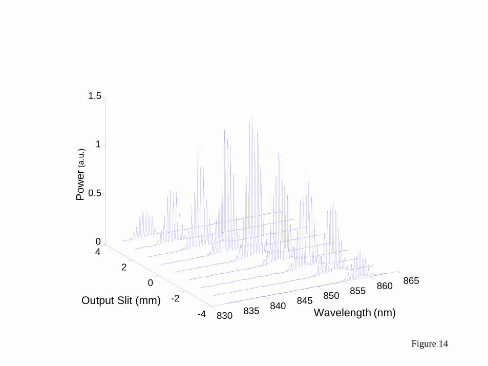
Figure 14

830 835 840 845 850 855 860 865

-4-2

02

40

0.5

1

1.5

Wavelength (nm)Output Slit (mm)

Pow

er(a

.u.)

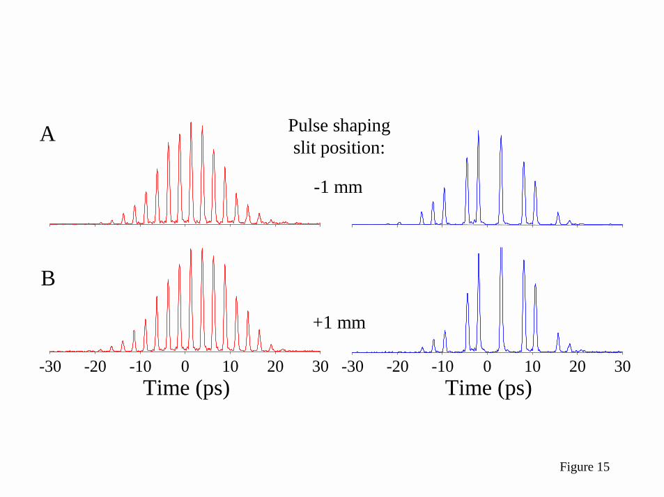
Figure 15

Time (ps)-30 -20 -10 0 10 20 30

Time (ps)-30 -20 -10 0 10 20 30

Pulse shapingslit position:

-1 mm

+1 mm

A

B