Embed Size (px)
Citation preview

DESIGN AND CONSTRUCTION OF A BRAIN MAGNETIC SIGNAL GENERATION PHANTOM FOR SOURCE
RECONSTRUCTION STUDY
by
Feng-yu Liu B.A.Sc., Simon Fraser University, 2008
THESIS SUBMITTED IN PARTIAL FULFILLMENT OF THE REQUIREMENTS FOR THE DEGREE OF
MASTER OF APPLIED SCIENCE
In the School of Engineering Science
Faculty of Applied Science
© Feng-yu Liu 2011
SIMON FRASER UNIVERSITY
Fall 2011
All rights reserved. However, in accordance with the Copyright Act of Canada, this work may be reproduced, without authorization, under the conditions for Fair Dealing. Therefore, limited
reproduction of this work for the purposes of private study, research, criticism, review and news reporting is likely to be in accordance with the law, particularly if cited appropriately.

APPROVAL
Name:
Degree:
Title of Thesis:
Examining Committee:
Chair:
Date Defended/Approved:
Feng-yu Liu
Master of Applied Science
Design and Construction of a Brain Magnetic Signal Generation Phantom for Source Reconstruction Study
Michael Sjoerdsma, Lecturer School of Engineering Science
Dr. Ash M. Parameswaran, P. Eng Senior Supervisor Professor, School of Engineering Science
Dr. Mirza Faisal Beg, P. Eng Supervisor Associate Professor, School of Engineering Science
Dr. Andrew Rawicz, P. Eng Internal Examiner Professor, School of Engineering Science
November 24.2011
ii

SIMON FRASER UNIVERSITY LIBRARY
Declaration of Partial Copyright Licence The author, whose copyright is declared on the title page of this work, has granted to Simon Fraser University the right to lend this thesis, project or extended essay to users of the Simon Fraser University Library, and to make partial or single copies only for such users or in response to a request from the library of any other university, or other educational institution, on its own behalf or for one of its users.
The author has further granted permission to Simon Fraser University to keep or make a digital copy for use in its circulating collection (currently available to the public at the "Institutional Repository" link of the SFU Library website <www.lib.sfu.ca> at: <http://ir.lib.sfu.ca/handle/1892/112>) and, without changing the content, to translate the thesis/project or extended essays, if technically possible, to any medium or format for the purpose of preservation of the digital work.
The author has further agreed that permission for multiple copying of this work for scholarly purposes may be granted by either the author or the Dean of Graduate Studies.
It is understood that copying or publication of this work for financial gain shall not be allowed without the author's written permission.
Permission for public performance, or limited permission for private scholarly use, of any multimedia materials forming part of this work, may have been granted by the author. This information may be found on the separately catalogued multimedia material and in the signed Partial Copyright Licence.
While licensing SFU to permit the above uses, the author retains copyright in the thesis, project or extended essays, including the right to change the work for subsequent purposes, including editing and publishing the work in whole or in part, and licensing other parties, as the author may desire.
The original Partial Copyright Licence attesting to these terms, and signed by this author, may be found in the original bound copy of this work, retained in the Simon Fraser University Archive.
Simon Fraser University Library Burnaby, BC, Canada
Last revision: Spring 09

ABSTRACT
Magnetoencephalography (MEG) is a powerful tool in measuring magnetic
fields associated with human brain activities, provided that a reliable inverse
analysis method is available for mapping the recorded magnetic field patterns to
active regions of neurons in the brain. The present study aims to develop a
method of physically generate magnetic field patterns of which the MEG data can
be used for developing a novel dipole localization technique. The mechanism of
generating specific magnetic field patterns consists of coils attached to individual
signal-generating circuits controlled by a central unit linked to a computer through
a standard USB port. This study explored various coil designs that generated the
simulated-brain magnetic dipoles. The use of triangular coils, as opposed to
magnetic dipoles generated by helical coils, was also studied.
The use of triangular coils was observed to have limitations in modelling
true dipoles. The inverse analysis technique developed in association with this
study showed high consistency in mapping the location and directionality of the
source dipoles.
Keywords: Magnetoencephalography; Magnetic fields; Inverse analysis; Dipole localization; Triangular coil; Current dipole; Signal-generating circuit; Mapping
iii

DEDICATION
I would like to dedicate this thesis to my family, without whose support I
could never have a chance to accomplish anything so far, especially to my
passed grandfather. His friendliness and kindness towards people around him
have always been my guidance towards life.
iv

ACKNOWLEDGEMENTS
I would like to specially acknowledge Teresa Cheung, the MEG laboratory
manager in DSRF Burnaby and Dr. Yoshinao Kishimoto, without whom this
project could never have been proceeded. I want to thank Teresa's kind
assistance on MEG measurement and Yoshinao's dedicated contribution on
inverse analysis portion of the project and provision of valuable knowledge.
Many thanks also go to Dr. Ash M. Parameswaran, my senior supervisor,
for his continuing support and guidance on my research, both academically and
personally. Thank you to Dr. Mirza Faisal Beg and Dr. Andrew Rawicz for
providing feedback to the work and sparing time for the defence. Thank you to
Mike Sjoerdsma for chairing the defence and his provision of inspirational
thinking throughout my study. Thank you to all my lab mates in microelectronics
lab for their frequent encouragement and provision of ideas. At last but not the
least, I thank the staffs at DSRF Burnaby for their generosity in granting me
access to the MEG lab.
v

TABLE OF CONTENTS
Approval ........................................................................................................................... ii
Abstract ........................................................................................................................... iii
Dedication ....................................................................................................................... iv
Acknowledgements ........................................................................................................ v
Table of Contents ........................................................................................................... vi
List of Figures .............................................................................................................. viii
List of Tables .................................................................................................................. xi
List of Abbreviations .................................................................................................... xii
1: Introduction ................................................................................................................. 1 1.1 Basics of Brain Neurons ........................................................................................... 1 1.2 Methods of Measuring Brain Activity ......................................................................... 3 1.3 Inverse Problem ........................................................................................................ 4 1.4 Objectives ................................................................................................................. 7 1.5 Thesis Outline ........................................................................................................... 9
2: Theory and Approach ............................................................................................... 10 2.1 Magnetoencephalography ...................................................................................... 10 2.2 Inverse Analysis ...................................................................................................... 13
3: Progression of the Project ....................................................................................... 15 3.1 Previous Implementation ........................................................................................ 15 3.2 Modified Design ...................................................................................................... 16 3.3 Further Improvement in Design .............................................................................. 23
4: Design of HardWare .................................................................................................. 24 4.1 Signal Emitting Mechanism ..................................................................................... 24 4.2 Control Electronics .................................................................................................. 25 4.3 Signal Filtering ........................................................................................................ 27
5: Design of Algorithm .................................................................................................. 32 5.1 Overall Design Structure ......................................................................................... 32 5.2 Graphic User Interface ............................................................................................ 34 5.3 Signal Generating Algorithm ................................................................................... 36 5.4 Frequency Calibration ............................................................................................. 42
vi

5.5 Embedded Control and Communication ................................................................ .44
6: Measurement and Analysis ...................................................................................... 50 6.1 Experiment and Method .......................................................................................... 50 6.2 MEG Measurement using Helical Coils .................................................................. 53 6.3 Simulated Magnetic Field Pattern of a Triangular Coil ............................................ 55 6.4 MEG Measurement using Triangular Coils ............................................................. 61
7: Conclusion and Future Work ................................................................................... 69 7.1 Conclusion .............................................................................................................. 69 7.2 Future Work ............................................................................................................ 69
Appendices .................................................................................................................... 71 Appendix A: Schematic Drawings ................................................................................... 72
Appendix A 1: Schematic of standalone waveform-generating unit in previous implementation ............................................................................. 72
Appendix A2: Schematic drawing of waveform-generating unit developed for this thesis work ............................................................................................ 73
Appendix A3: Schematic drawing of the MUXlDeMUX circuit ................................ 74 Appendix B: Matlab Code for Waveform-composing GUI ............................................... 75 Appendix C: C++ Code for Interactive Host GUI ............................................................. 85 Appendix D: C++ Code for AT90USB1287 Microcontroller Firmware ........................... 102 Appendix E: Assembly Code for Programming ATMega32 Microcontroller .................. 108 Appendix F: Simulated Magnetic Field Patterns ........................................................... 121
I. Z-component with triangular coils of 5-mm base length and various leg lengths ....................................................................................................... 121
II. V-component with triangular coils of 5-mm base length and various leg lengths ....................................................................................................... 122
III. Z-component with equilateral triangular coils of various side lengths .............. 123 Appendix G: Inverse Analysis Results .......................................................................... 124
Reference List ............................................................................................................. 126
vii

LIST OF FIGURES
Figure 1.1: Procedures of studying brain neuronal activities and the emitted magnetic fields .................................................................................................. 5
Figure 1.2: Study of inverse analysis methods by replacing the human subject with a magnetic-field-emitting device ................................................................ 8
Figure 2.1: Sensing mechanism of (a) axial gradiometer and (b) Planar gradiometer ..................................................................................................... 11
Figure 2.2: (a) SQUID sensors and a liquid helium Dewar and (b) MEG signal processing electronics at Burnaby DSRF ....................................................... 13
Figure 2.3: Procedures of inverse analysis on measured MEG data ........................... 14
Figure 3.1: (a) "Wet phantom" consisting of a pair of electrodes at the end of a twisted wire pair immersed in electrolyte and (b) illustration of flow of ions completes the current loop inside ~ wet phantom ................................... 15
Figure 3.2: Hardware configuration of the previously implemented magnetic-signal-generating electronics .......................................................................... 17
Figure 3.3: Control algorithm of the magnetic-signal-emitting electronics (previous implementation) .............................................................................. 18
Figure 3.4: (a) Helical coils mounted on a plastic base. (b) Test coils placed in the SQUID measurement cavity inside a magnetically shielded room ........... 20
Figure 3.5: Magnetic flux density recorded at MEG channels when (a) a rectangular waveform and (b) a sinusoidal waveform was used as the source signal ................................................................................................... 21
Figure 3.6: Spatial magnetic flux density distribution when (a) 2 helical coils (b) 4 helical coils were energized simultaneously ................................................ 21
Figure 3.7: (a) Magnetic flux density distribution after truncated singular value decomposition (TSVD) was applied. (b) Localized dipoles after cluster analysis was applied to the TSVD result and after down simplex method (DSM) was applied to the cluster analysis result. .............................. 22
Figure 4.1: Modified design of the overall simulated-brainwave-generating electronics ....................................................................................................... 26
Figure 4.2: Dataflow among components in a signal generating unit. ......................... 27
Figure 4.3: Unfiltered sinusoidal signal at the output (Vpk-pk = 3.2 V, period = 81 ms) .................................................................................................................. 28
Figure 4.4: Resulting cutoff frequency in comparison with the input cutoff frequency of the implementation ..................................................................... 30
viii

Figure 4.5: (a) Magnitude response and (b) phase shift of the output filter ................. 30
Figure 4.6: (a) Unfiltered and (b) filtered signals at the output (Vpk-pk = 2.78 V, period = 9.7 ms) .............................................................................................. 31
Figure 4.7: Frequency spectra of (a) unfiltered and (b) filtered signals ....................... 31
Figure 5.1: Overall representation of data exchange between interconnected control algorithm blocks .................................................................................. 33
Figure 5.2: Graphic user interface for composing the output signal waveform (programmed in Matlab) ................................................................................. 35
Figure 5.3: Real-time interactive graphic user interface dialog on host PC ................. 35
Figure 5.4: Control algorithm of the Matlab GUion host PC ....................................... 37
Figure 5.5: Implementation of the signal generating algorithm of SGU ....................... 38
Figure 5.6: Representation of a sinusoidal signal (a) 3 times and (b) 10 times of the coexisting fundamental frequency, both with 32 quantization coefficients ...................................................................................................... 40
Figure 5.7: A sinusoidal signal composed of different numbers of quantization coefficients ...................................................................................................... 40
Figure 5.8: Frequency spectra of an unfiltered sinusoidal signal of 100Hz fundamental frequency formed with (a) 32, (b) 64, (c) 128, and (d) 256 quantization coefficients ................................................................................. 41
Figure 5.9: Relationship between resulting frequency of the output sinusoidal signal and the input value of frequency for different number of quantization coefficients before frequency calibration ................................... .43
Figure 5.10: Relationship between resulting frequency of the output sinusoidal signal and the input value of frequency after frequency calibration ................ 44
Figure 5.11: Data structure of the stored parameters for each individual channel on host PC ........................................................................................ 46
Figure 5.12: Structure of the packets sent from host PC to CCU during each data transfer .................................................................................................... 46
Figure 5.13: Command-decoding algorithm on each SGU ....................................... .47
Figure 5.14: Communication states of data point forwarding from CCU to SGU ................................................................................................................ 49
Figure 6.1: (a) A helical coil (3 loops) and (b) an isosceles triangular coil fixed on a wooden stick. The distance between two adjacent marked lines on the stick is 1 cm ......................................................................................... 50
Figure 6.2: (a) Front view, (b) left-side view, and (c) right-side view of coil placements on a plastic skull covered with a layer of rubber sheet mounted on a plastic base .............................................................................. 51
Figure 6.3: Final assembled magnetic-field-emitting circuit.. ....................................... 52
Figure 6.4: Polhemus FASTRAK® 3D Digitizer used for localizing points in 3D space, including a transmitter and a receiver fixed around the test skull
ix

during the experiment and a stylus used for physically locating the coils on the skull. ............................................................................................ 53
Figure 6.5: Relative locations of the helical coils on the head surface ........................ 53
Figure 6.6: Frequency spectra of (a) all coils at 13 Hz, maximum current and (b) all coils at 13 Hz, minimum current. .......................................................... 54
Figure 6.7: Frequency spectra of (a) coil 4 at 50 Hz, the rest at 13 Hz, half current and (b) coil 4 at 50 Hz, coil 7 at 90 Hz, the rest at 13 Hz, half current. ............................................................................................................ 55
Figure 6.8: Example triangular coil model constructed in COMSOL. ........................... 56
Figure 6.9: Simulated space in COMSOl, consisting of a cube of 10-cm side length .............................................................................................................. 57
Figure 6.10: (a) Z-component on xy-plane (z = 5 cm), (b) y-component on zx-plane (y = 5 cm), and (c) x-component on yz-plane (x = 5 cm) of the magnetic field generated by the simulated triangular coils ............................. 58
Figure 6.11: Max z-component magnetic flux density in the xy-plane at z = 5 cm from origin of isosceles triangular coils ..................................................... 59
Figure 6.12: Y -component magnetic flux density in the zx-plane at y = 5 cm (x = 0, z = 0) from origin of isosceles triangular coils .......................................... 60
Figure 6.13: Max magnetic flux density in the plane perpendicular to the axial component at 5 cm from origin of equilateral triangular coils ......................... 61
Figure 6.14: Relative locations of the triangular coils on the head surface ................ 62
Figure 6.15: Spatial distribution of sensors around the measured space, for a total of 151 channels, each having an inner and an outer sensors ................ 63
Figure 6.16: Spatial magnetic flux density distribution of test cases 1, 2, 5, 11 at time equal to 1.1 seconds after the start of recording (Unit: IT) .................. 64
Figure 6.17: AC component of the recorded magnetic flux densities on all channels for test cases 1, 2, 7, 8, 10, and 11 ................................................. 65
Figure 6.18: left - Resulting magnetic flux density distribution after TSVD; middle - Resulting dipole locations after data clustering; rightAdjusted dipole locations after downhill simplex computation of test cases 5,8, and 9 ............................................................................................ 67
x

LIST OF TABLES
Table 6.1: Measured base and side lengths of different types of triangular coils used in the experiment. .................................................................................. 62
Table 6.2: Coils energized in different test cases in the experiment. .............................. 63
Table 6.3: Resulting dipole moments for the dipole associated with each coil across different test cases from the inverse analysis and their correlation ....................................................................................................... 68
xi

LIST OF ABBREVIATIONS
MEG Magnetoencephalography
PET Positron emission tomography
fMRI Functional magnetic resonance imaging
DAC Digital to analog converter
EEG Electroencephalography
ECD Equivalent current dipole model
SQUID Superconducting quantum interference device
AICC
TSVD
CCU
SGU
GUI
Akaike information criterion for small sample sizes
Truncated singular value decomposition
Central control unit
Signal generating unit
Graphic user interface
xii

1: INTRODUCTION
1.1 Basics of Brain Neurons
The human brain, the most critical part of the central nervous system,
contains mostly interneurons, which integrate and analyze signals sent from
sensory neurons and send signals to the motor neurons to perform response in
accordance to the environmental stimuli [1,2]. The highly evolved ability of
information integration and interpretation by the human brain is reflected by the
highly complex interconnection among interneurons in the brain. Neurons are
composed of three major structures: the dendrite, the cell body, and the axons.
The neuron cell membrane is impermeable to charged particles. In the resting
state, the inside of a neuron cell contains a higher concentration of K+ and a
lower concentration of Na+ compared to the extracellular environment, and the
bilayer structure of the cell membrane contributes to maintaining the ion
gradients caused by the difference in charged particle concentrations. The Na+
and K+ gradients maintained across the membrane are mainly responsible for the
activation of a neuron. Upon receiving signals from other neurons by the
dendrites, the axon of a neuron transmits signals to other neurons. The stimulus
received by a neuron causes transmembrane proteins called ion channels to
open up and thus increases the permeability of the membrane. The propagation
of a nerve pulse within a neuron results as Na+ and K+ ions are passed in and out
of the neuron down their concentration gradients through gated ion channels
1

located on the cell membrane. After each activation process, the resting potential
of the neuron is restored by the cell actively pumping these charged particles
across the membrane against their concentration gradients. The membrane
potential of a neuron that is constantly stimulated by the signal from a sensory
receptor consists of a pulse train of action potentials. The freuqncy of the pulse
trains is dependent upon the magntidue of the stimulus the sensory receptor is
exposed to. The stronger the external stimulus, the shorter the time interval
between adjacent action potential pulses is on the neuron.
Any cognitive and thinking process or environmental stimulation may
trigger the change of membrane potential in certain neurons [3]. Through this
membrane depolarization-repolarization process, an action potential is created
once the magnitude of membrane potential reaches a particular threshold value
and the electrical signal is passed down the axon of the neuron. The relay of
signals between two adjacent neurons is achieved by the release of
neurotransmitters across the gap junction between the transmitting axon of a
neuron and the receiving dendrite of the next neuron. The combination of the
action potential and neurotransmitters results in the relay of signals across the
nervous system. The current and its corresponding magnetic field generated by
the flow of charged particles when neurons are active in the human brain form
the basis of the present study.
2

1.2 Methods of Measuring Brain Activity
Research on human cognitive behaviours and their corresponding regions
of neurons activated in the brain finds its application in various fields of study,
including psychology, cognitive science, and clinical science. Moreover, the
correlation between given cognitive processes and the resulting brainwave
patterns is also subject to intense study. Various methods have been developed
for the detection of neuronal activities in human brains. Commonly employed
methods include positron emission tomography (PET), functional magnetic
resonance imaging (fMRI), electroencephalography (EEG),
magnetoencephalography (MEG), and etc .. Both PET and fMRI provide good
spatial resolution but relatively poor temporal resolution compared to EEG and
MEG, on the order of seconds or more. PET and fMRI are capable of generating
high-resolution 3D images [4, 5]. However, as opposed to EEG and MEG, the
present technology limits PET and fMRI for continuous recording of neuronal
activity over a substantial period of time. EEG and MEG are capable of resolving
temporal precision on the order of milliseconds. Furthermore, PET requires the
test subject to be pre-treated with radioactive tracer molecules, which would
increase the risk of damaging bio-tissues. EEG measurement, accomplished by
placing electrodes that record electrical potentials at fixed locations on the scalp,
is limited by the poor conductivity of the skull. It greatly increases the difficulty to
locate the source of neuronal activity. Meanwhile, the magnetic fields not
attenuated by the skull and other tissues make MEG a more effective method in
spatially localizing the sources in the brain compared to EEG [6]. In addition,
3

MEG is a completely non-invasive method because the sensors do not make
direct contact with the head. MEG, due to its high spatial resolving capability, is
often performed in conjunction with EEG due to their complementary measuring
capabilities, since the fields detected by these two methods are mutually
orthogonal. MEG detects mainly the activities in the cortical fissures. Notably, it
is the intracellular post-synaptic potentials on active pyramidal neurons that MEG
detects, not the potentials created by the polarization-depolarization process
within the neurons [7].
1.3 Inverse Problem
In electromagnetism, when the source that generates a magnetic field is
initially known, such as the location, orientation, and current density of a current
dipole, the resulting distribution of the magnetic flux density can be easily
computed using Biot-Savart law and Maxwell's equations. Such a procedure of
determining the magnetic field from a given electrical field is a forward problem.
However, in the study of biomagnetism, inverse problems are often involved,
when the information of locations, magnitudes, and numbers of individual dipoles
are initially unknown, while only measured distribution of magnetic flux densities
is available. Figure 1.1 illustrates the procedures of studying the pattern of
magnetic fields generated by brain neuronal activities.
4

Cognition & Acitve Thinking
Induction
Exchange of Ions (Electrical Signal)
Magnetic Fields (Measured Quantity)
Inverse Analysis
Figure 1.1: Procedures of studying brain neuronal activities and the emitted magnetic fields.
In a MEG recording with a human subject, very often the resulting
magnetic field distribution can be modelled as the equivalent current dipole
(ECD) model [8, 9]. The brain-induced magnetic field that is measured by MEG is
[10]:
(1 )
! is the impressed current density resulting from neuron cellular bioelectricity,
equivalent to the source volume dipole moment density if the ECD model is used.
The OJ'''-Oj''term, being the conductivities of different materials, accounts for any
inhomogeneity of the volume conductor. Single-dipole model assumes
5

synchronous activation of a group of functionally interconnected neurons which
are closely located in the cerebral cortex, for a given neuron-triggering event.
Nonetheless, when the resulting distribution of magnetic field involves multiple
individually activated brain neuron groups or large patches, the single-dipole
model would be less suitable in estimating the location of the sources [3, 11]. In
such cases, multidipole models should be used to give accurate estimation of the
source dipoles. The study of inverse analysis of MEG data is usually combined
with EEG and fMRI, since EEG detects all primary current components, while
MEG only detects the tangential components. Meanwhile, fMRI or other
tomography methods are capable of providing higher spatial resolutions.
Brain activity reconstruction typically involves forward modelling
components including the source model, the volume conductor model, and the
measurement model, together with the reconstruction algorithm for inverse
modelling [12]. Various inverse algorithms including the commonly adapted
minimum-norm estimates have been demonstrated to give good source-current
localization result and often depend largely on the accuracy of the a priori
information [13, 14]. Given a set of MEG data recorded, the general approach for
localizing the sources of dipoles using inverse analysis is to make an initial
assumption about the location and number of individual dipoles based on the
data. Then the error between the estimation and the actual measured data needs
to be minimized by iterative computation to yield the best approximation of the
sources of the measured magnetic field.
6

1.4 Objectives
The study of the inverse problem on the MEG data using human subjects
is significantly deterred by the lack of the ground truth about the actual location
and orientation of the dipoles. The main problem of using a human subject for
MEG data collection is the actual location of source dipoles, which are
associated with the neuronal activities in particular regions of the brain. This can
only be estimated in conjunction with methods such as fMRI, due to the fact that
normal humans do not have voluntary control over the groups of brain neurons to
be activated. However, if the magnitude, location, and orientation of the dipole
sources are initially known, together with the measured MEG data, the accuracy
of a particular inverse analysis technique can be evaluated. Moreover, study
using human subjects is more prone of noise due to the movement of the head or
limbs and the magnetic fields produced by the heartbeats and pulses.
Constructing realistic brain phantoms have been attempted for assisting the
inverse analysis study of EEG and MEG data [15-18]. In the present study, a
brain phantom is constructed to replace human subjects, in attempt to serve
physical simulation of magnetic field emitted by brain neuronal activities for
inverse analysis study, as shown in Figure 1.2. More specifically, such a
phantom is to be used for assisting the development of a dipole localization
technique by providing control over the pattern of the magnetic fields produced
and the orientation and location of each individual dipole. Furthermore, the noise
introduced by the simulation circuit can also be characterized and attenuated.
Eventually, the objective of the inverse analysis technique development is to
7
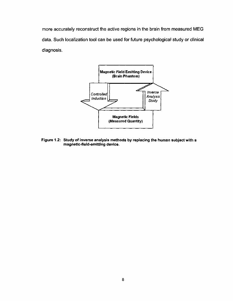
more accurately reconstruct the active regions in the brain from measured MEG
data. Such localization tool can be used for future psychological study or clinical
diagnosis.
Magnetic Field Emitting Device (Brain Phantom)
Magnetic Fields (Measured Quantity)
Inverse Analysis Study
Figure 1.2: Study of inverse analysis methods by replacing the human subject with a magnetic-field-emitting device.
8

1.5 Thesis Outline
The study presented in this thesis focuses on developing a method of
physically simulating magnetic fields emitted by the human brain (brain
phantom), as well as how the brain phantom can be used for developing a novel
inverse analysis method. Chapter 2 provides a brief overview on the principles of
magnetoencephalography and its operational mechanism. Chapter 3 covers the
progression of the current project and earlier development of the present project.
Chapters 4 and 5 provide details of implementation of the current brainwave
simulating mechanism in hardware and software aspects, respectively. Chapter 6
outlines experimental procedures of recording magnetic fields generated using
the brain phantom developed and results of the inverse analysis technique
developed. Finally, a conclusion and future work are outlined in the last chapter.
9

2: THEORY AND APPROACH
2.1 Magnetoencephalography
Magnetoencephalography measures the biomagnetic signals associated
with the movement of charged particles in active brain neurons. The problem
mostly encountered in the measurement of human brain signal is the relatively
weak magnitude of the signal of interest [4, 19]. The magnetic field produced by
brain neuron activities is often orders of magnitude weaker than background
magnetic interference, including the earth's magnetic field. The typical urban
background noise, which may include the magnetic fields generated by electric
power lines and geomagnetic field fluctuations, could be in the order of
microteslas, while the magnetic fields generated by human brain activities are in
the range of picoteslas. The measurement of human brain signal requires
superconducting quantum interference device (SQUID), which has extremely
high sensitivity in detecting the magnetic field of the brain [20]. A typical SQUID
system consists of a flux transformer connected to the SQUID electronics. The
flux transformer is composed of a gradiometer and a SQUID assembly. At the
output of the system, the SQUID electronics renders a voltage signal whose
magnitude is proportional to the amount of magnetic flux sensed by the
gradiometer. The gradiometer, which functions as a sensor in detecting the
magnetic field signals, is connected to the input coil of the SQUID assembly.
Liquid helium cooling is required for the flux transformer, of which the
10

implementation is based on the Meissner effect and Josephson effects of
superconductors [21]. Usually, the measurement needs to be conducted in a
heavily magnetically shielded environment to further attenuate the interference of
the background noise. The principle of detection relies on the different
homogeneities of magnetic signals from different sources. In a properly
magnetically shielded space, while the magnetic field generated by the human
brain weakens as the distance from the source increases, the background
magnetic signals are mostly homogeneous across the gradiometer antennae [10,
21]. A SQUID gradiometer is designed to detect the brain magnetic field from the
discrepancy in magnetic flux densities caused by the distance. Figure 2.1
illustrates the mechanism of magnetic field sensing of the first-order gradiometer.
".,." '"~-~~~"";;:>"'.''''-,
{/ Ma£netlc
Source \
(a) (b)
Figure 2.1: Sensing mechanism of (a) axial gradiometer and (b) Planar gradiometer.
11

Located at the Down Syndrome Research Foundation,1 the MEG system
manufactured by CTF System is capable of measuring 151 channels, formed by
individual axial gradiometers. These 151 gradiometers are spatially distributed to
cover the whole brain cortical system and are capable of sensing magnetic field
emitted by most of the regions in the human brain cortex. The MEG system is
equipped with two environmental noise reduction methods. Noise reduction can
be achieved either by higher-order gradiometer formation or by adaptive filtering
or both. Higher-order gradiometer noise cancellation employs hardware
mechanism while keeping the filter coefficient static. Adaptive filtering, on the
other hand, is implemented via signal processing approach using variable
filtering coefficients [22]. The change of the coefficients depends on the
environment. As shown in Figure 2.2 below, located in a magnetically shield
room, the magnetic signal emitting test subject is fitted inside the cavity
surrounded by the gradiometers together with the liquid helium containing Dewar.
The signal processing electronics of MEG, meanwhile, is located outside of the
room to minimize the noise emitted by the MEG circuits.
1 Down Syndrome Research Foundation is a registered non-profitable charity focusing on both servicing the community and researching Down Syndrome. It is located at 1409 Sperling Avenue, Burnaby, Be V5B 4J8
12

Figure 2.2: (a) SQUID sensors and a liquid helium Dewar and (b) MEG signal processing electronics at Burnaby DSRF.
2.2 Inverse Analysis
The novel inverse analysis method for localizing the dipoles in the present
study was developed by Kishimoto [23]. As shown in Figure 2.3 below, the
method consists of two major phases: extracting phase and grouping phase. In
the data extracting phase, in which the magnitude distributions of the dipoles are
to be determined, truncated singular value decomposition (TSVD) is applied to
the MEG data recorded using Akaike information criterion for small sample sizes
(AICC) repeatedly. In the grouping phase, the distributions of the dipoles are
grouped by data clustering before downhill simplex computation are applied to
these groups of data for optimizing the locations of these dipoles.
13

l MEG data I
... Extracting phase: iterative TSVD and AICC
" I Magnitude distributions of dipoles
Grouping phase: ... data clustering and ~
downhill simplex computation
~
I Representative dipoles
Figure 2.3: Procedures of inverse analysis on measured MEG data.
14

3: PROGRESSION OF THE PROJECT
3.1 Previous Implementation
An electrolyte-based electromagnetic signal-emitting device was
previously constructed to physically generating magnetic signal. Such a device
consisted of a control electronic circuit connected to a symmetrical twisted pair of
wires ended as a pair of electrodes immersed in a saline solution, which
functioned as the medium for ion exchange, as shown in Figure 3.1. The twisted
pair of wires had insulated coating except at the tips which function as the
electrodes.
(b)
Figure 3.1: (a) "Wet phantom" consisting of a pair of electrodes at the end of a twisted wire pair immersed in electrolyte and (b) illustration of flow of ions completes the current loop inside a wet phantom.
The previous version of control electronics was developed by Simon
Fraser University research group for generating basic waveforms such as
15

sinusoidal signals with one frequency component. The control circuit included
mainly a microcontroller with two 8-bit digital-to-analog converters (DAC's)
attached. One of the two DAC's was used as a reference DAC for fixing the input
voltage level of another DAC, the output DAC. While the DAC's lacked memory
components and could not be programmed, a microcontroller was required for
dictating the output voltage of the output DAC. The microcontroller was
programmed with 32 predefined 8-bit coefficients, ranging from 0 to 255 in
decimal for composing the output waveform. These 32 coefficients defined the
shape of the waveform to be output to the coil. Sequentially, each of these
coefficients was transferred one-by-one from the microcontroller to the output
DAC, which synchronously generated the corresponding voltage level. The signal
generated by the DAC was transmitted to the twisted pair of wires, and the pair of
wires, together with the saline solution, formed a closed loop for the current
sourced by the DAC chip to flow, as shown in Figure 3.1 above. In this case, the
saline was the electrolyte, in which the ion exchange allowed the charges in the
wires to be transferred. Due to the symmetrical configuration of the twisted pair,
the magnetic field emitted by each wire in the twisted pair was largely cancelled
out, and only the ion exchange between the twisted pair in the electrolyte and the
current carried by the two arms of electrodes would contribute to a measurable
magnetic field.
3.2 Modified Design
The design elaborated above was not with its limitations. First, the
electronic design allowed only limited signal generating capability. In addition to
16

only one set of waveform coefficients that could be defined each time, the
microcontroller had to be re-programmed using a development board provided by
Atmel®, whenever an alteration of the waveform parameters, such as the
amplitude or the frequency, was required. Such programming procedures,
involving the un-mounting and mounting of the microcontroller on the
development board, tend to be laborious if frequent change of the waveform
parameters is needed during the operation of the device. Moreover, the
electronic parts are more prone to damage by electrostatic charges when
frequent mounting and un-mounting of the microchips are performed.
Conlrol User Contr(jled
Amplitude & f---- InputADC Dala
Frequency r---
MlerIXontroller
t:0l
Digital Amplitude
Data Display LED r-- & Frequency Display
Conlrol Output DAC ~ Coli r-- Output Analog WavefOrm
Figure 3.2: Hardware configuration of the previously implemented magnetic-signa 1-generating electronics.
To improve on the issues mentioned above, it was necessary to design
control electronics that allowed the waveform parameters to be updated without
re-programming the microcontroller [24]. The hardware was constructed using
17

electronic blocks shown in Figure 3.2. See Appendix A 1 for the detailed
schematic. To accomplish this, a voltage and amplitude input control elements
were integrated to the circuit using analog-to-digital converters (ADC's) and
potentiometers. Also the corresponding display elements were implemented
using 7 -segment LED displays. The microcontroller was programmed to
periodically sample and display the input values of these waveform parameters
and adjust the DAC's to generate waveforms defined by the specific parameters,
following the algorithm shown in Figure 3.3.
Generating voltage accord ing to the indexed positio n in th e waveform
N
Figure 3.3: Control algorithm of the magnetic-signal-emitting electronics (previous implementation).
18

Furthermore, the use of liquid electrolyte as the conducive medium
between the twisted pair of wires, though might more physically resemble the ion
exchange occurring in each individual neuron in a human brain, would incur
interference, if the number of twisted pairs of wires increases. One problem for
using saline water in the construction of a brain phantom is the nonlinearity
between the source signal and the measured magnetic field due to the electrical
double layer around the electrodes in the saline water [25]. The electrical double
layer occurs in the pre-electrolysis process due to the minimum energy required
for the electrolysis of the saline molecules to begin. Another problem would arise
if the distance between two pairs decreases, as the number of twisted pairs
increases, given that they all share the same liquid conductive medium. To form
a complete loop of electrical charge flow, the amount of current carried by the
pair of wires has to be replaced by the equivalent amount of charges exchanged
in the electrolyte at the ends of the twisted pair of wires immersed in the saline.
Since the direction of ion flow in the electrolyte is not restricted as the flow of
electrons in a conductive wire, the majority to the ions would take the shortest
paths between the source and the sink of the electrical charges. When the
distance between individual twisted pairs becomes comparable to the distance
between the two electrodes of each individual wire pair, as the number of wire
pairs increases, interference due to the cross-flow of charges would be expected.
For allowing a larger number of dipoles to be generated simultaneously
without cross-interference among individual dipoles, small coils combined with
twisted pairs of wires were used, termed "dry phantom", as opposed to the "wet
19

phantom" previously described, which has twisted pairs immersed in liquid
electrolyte.
In the previous MEG measurement conducted [24, 26], using the
brainwave simulating circuit aforementioned to provide signals, helical coils were
properly mounted on a plastic base, as shown in Figure 3.4. In this case, each of
the coils was positioned at approximately equidistance from the centre of the
base. Then the base was positioned inside the measurement cavity of the MEG,
located inside a magnetically shielded room.
Figure 3.4: (a) Helical coils mounted on a plastic base. (b) Test coils placed in the SQUID measurement cavity inside a magnetically shielded room.
The magnetic flux density recorded by multiple gradiometers over a time
period is shown in Figure 3.5 using the brain phantom constructed. The observed
multiple traces at a given time are due to the superimposition of the recordings
by multiple gradiometers. A sinusoidal and a rectangular waveform source signal
are shown for example. It can be observed that the magnetic field patterns are
consistent with the original source signal waveforms. The amount of current j
20

carried by an N-turn helical coil of constant loop area A governs the magnetic
field strength according to the relationship [27]:
Be ) - Jlo NiA Z ---
21l' z3 (2)
and can be adjusted accordingly to fit the range of magnetic field required for the
experiment.
4
£ 2 .~ J 0
~ -2 u 'il -4
I -6
x 1()4
0.0 0.2 0.4 0.6 0.8 1.0 Time [8] (a)
X 10 4
3
§ 1.5
.~ .: ., '" >( 0 :> C
<> .~
&, -1.5 '" ::>:
-3 0.8 1.0 1.2
Time [sj
Figure 3.5: Magnetic flux density recorded at MEG channels when (a) a rectangular waveform and (b) a sinusoidal waveform was used as the source signal.
[IT]
300 2r----.----.-----r---.,
150
o ~ 0 "<
-150 -I
-300 -2
2 0 -I -2 X [rad] (a) )' [rad] (b)
1.4
(b)
2
0
-I
-2
Figure 3.6: Spatial magnetic flux density distribution when (a) 2 helical coils (b) 4 helical coils were energized simultaneously.
21

Meanwhile, the planar view of the spatial distribution of the resulting
magnetic flux density at a particular time instance is shown in Figure 3.6. The
inverse analysis method described above was applied to the magnetic flux
density data measured by the MEG gradiometers. The resulting magnetic field
distribution after TSVD was applied is shown in Figure 3.7. Figure 3.7 also
displays the localization results of dipoles after data clustering analysis and
downhill simplex method were applied, respectively.
100
50
I 0 ........ N
-50
-100
-50 o
50 x [mm] 100
100
50
o
-50
-100
-50 o
50 x [mm] 100
~ Actual
----7 TSVD
100
y[mm] (a)
~ Actual
-----0---0> Cluster analysis
~ DSM
100
y[mm] (b)
Figure 3.7: (a) Magnetic flux density distribution after truncated singular value decomposition (TSVD) was applied. (b) Localized dipoles after cluster analysis was applied to the TSVD result and after down simplex method (DSM) was applied to the cluster analysis result.
22

3.3 Further Improvement in Design
A more advanced version of brain phantom can be implemented by
introducing a graphic user interface that renders the visualization of the
waveform shape to be generated. Furthermore, the device needs to allow an
arbitrary signal waveform to be defined without having to re-program the control
algorithm of the microcontroller. The rest of the thesis focuses on the
development of an improved mechanism for creating more complex magnetic
signals in attempt to more realistically simulate the electromagnetic fields emitted
by human brain neurons. Such approach is to be used for further improving the
inverse analysis technique developed in association with this study.
23

4: DESIGN OF HARDWARE
4.1 Signal Emitting Mechanism
A magnetic field can be generated by applying electric signals to a coil
attached to the output of a signal generating circuit via a twisted pair of wires,
which ensures a detectable magnetic field is created only in the vicinity of the coil
but not along the pair of current conducting wires. Conventionally, magnetic fields
are produced by using a solenoid, a tightly wound helical coil of wire, which can
be modelled as a magnetic dipole. However, the ion exchange associated with
neuronal activities is more realistically modelled as the emergence of current
dipoles. The study of the novel dipole localization method in the present research
attempted both approaches by using both helical coils and triangular coils.
As previously mentioned, the use of a symmetrical twisted pair of wires
immersed in saline water provides an eligible model of a current dipole. The use
of isosceles-triangle coils in constructing the brain phantom was proposed to
provide several advantages [28]. Using a triangular coil eliminates the need of
liquid medium for ion exchange while still providing a similar electrical current
path. Not using electrolyte to form a circuit loop eliminates the non-linearity
between the generated magnetic field and the applied voltage and achieves
higher mechanical accuracy. Moreover, it provides more simplicity for the
experimental setup and eliminates the problem of electrode degradation.
24

4.2 Control Electronics
The requirement of a graphic user interface that facilitates the real-time
control of the waveform generation can be met by integrating a computer to the
design. The concept of the design involves a computer connected to a central
control unit (CCU) that distributes waveform parameters and control commands
to an intended waveform-generating unit. Figure 4.1 demonstrates the block
diagram of the design. Notably, as shown in Figure 4.1, the communication
established between the host PC and the CCU developed using the protocol
supplied by Atmel® allows bidirectional packet transfer. This feature can be
exploited to ensure that the CCU correctly receives the data issued by the host
PC during the implementation. On the other hand, the unidirectional data transfer
between the CCU and each channel is limited by the different logic voltage levels
between them. More specifically, logic level '1' has a voltage level of 3.3 Von the
CCU, while logic level '1' on each waveform-generating circuit has a voltage of 5
V. This difference in voltage level presents a limitation on the speed of the circuit,
which, however, is not of top priority at the present stage.
25

Host PC
~~ -01 Q)c: ~ro (.).c ro <.> 0.. x
~7
Central Control Unit (CCU)
"'o~ ro '-- -ro c: 0 0
() ... ~ ... ,..
Multiplexing/Demultiplexing Interface
"'- ~ "'-"" .. -~ ro e ro e
~ e
(U - (U "E "E c: ro 0 0 0 0 0 0
() () () ... ;,.. ... ;,.. ... ;,.. ... ". "" ~ ... ~
Waveform Waveform Waveform Generating Generating ........... . . . Generating
Unit 1 Unit 2 Unit N
Figure 4.1: Modified design of the overall simulated-brainwave-generating electronics.
The CCU that facilitates the communication between the host computer
and the peripheral, and the management of the data and instructions sent by the
computer is implemented using an AT90USBKEY board supplied with
A T90USB 1287 microcontroller by Atmel®. The board was specifically designed
to allow fast data transfer between the host PC and the on-board microcontroller.
The communication between the host computer and the AT90USBKEY is
established through USB ports on both the host and the receiving AT90USBKEY.
Upon receiving the data, the CCU distributes them to the microcontroller of a
specific waveform-generating unit (WGU) through a demultiplexing circuit (Refer
26
to Appendix A3 for detailed layout of the circuit) consisted of stacks of quad 2-
channel multiplexer/demultiplexer microchips (MC14551). The use of a
demultiplexing circuit introduces expandability to the design at the expense of
response time. The limitation of such implementation is that the more layers the
network contains, the longer it takes the signal to propagate from the CCU to
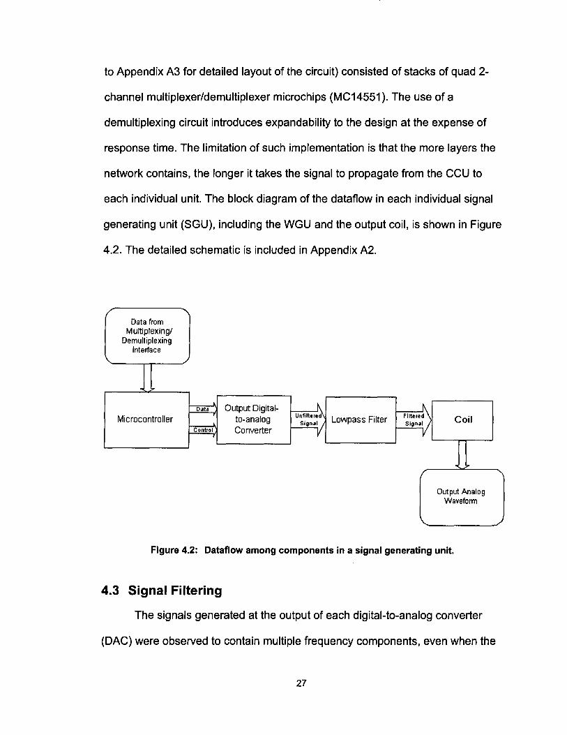
each individual unit. The block diagram of the dataflow in each individual signal
generating unit (SGU), including the WGU and the output coil, is shown in Figure
4.2. The detailed schematic is included in Appendix A2.
/' Data from
Multiplexing! Demultiplexing
Interface
Output Digital- unfilter~ Filtere-!\ Data
Microcontroller to-analog Lowpass Filter Coil Control Converter
Signa V SignV
.. .. /" "
Output Analog Waveform
'-. ./
Figure 4.2: Dataflow among components in a signal generating unit.
4.3 Signal Filtering
The signals generated at the output of each digital-to-analog converter
(DAC) were observed to contain multiple frequency components, even when the
27

intended signal was a sinusoidal function of single frequency component. This
was attributed to the method by which the signal was produced. Figure 4.3
shows an example of an unfiltered output signal of the DAC. Instead of a desired
smooth sinusoidal signal, the signal exhibited step-like slope. Such a signal could
be inferred as a mixture of a low-frequency pure sinusoidal signal and a high-
frequency step function, while the step function signal was composed of a wide
range of frequencies. Since this unfiltered signal contained the unwanted high-
frequency portion added to the signal to be generated, an output lowpass filter
was used to remove the unwanted frequency components.
1l .!L D Trig'd M Pos: 0.0005 HORIZONTAL ~~~~~~~~~~~~~~~
.. .. . . . . . . . . . . . . . . . . . . . . . . . . . _ ....................... . · . . . - . . . . · . . . - . . . . · . . . - . . . . · . . . - . . . . ........................ -....................... . · . . . - . . . . · . . . -. .. · . . . - .. . .-
· . . . _. .. ., ...................... _ ....................... . 1
· . . . - . . . . · . . . - . . . . · . . . - . . . . · . . . - . . . . ........................ _ ..................... '" · . . . - . . . . · . . . - . . . . · . . . - . . . . · . . . - . . . .
Window Zone
Window
Trig Knob
Hl!IIt 500.0ns
CH1 1.00V M 10.0ms CH1 f 2.32V 12.3546Hz
Figure 4.3: Unfiltered sinusoidal signal at the output (Vpk-pk = 3.2 V, period = 81 ms).
A fourth-order Butterworth low-pass filter was implemented by cascading
two second-order switched-capacitor filter blocks. Using an L TC1 060 switched-
capacitor filter chip by Linear Technology, the cut-off frequency of this low-pass
filter is adjustable based on the frequency of the input clock signal. In the present
implementation, the clock signal for the low-pass filter is generated using a pin on
28

the same microcontroller used for controlling the DAC. The particular pin
selected was dedicated to the output of a built-in counter on ATMega32. Figure
4.4 demonstrates the relationship between the input and resulting cut-off
frequencies of the low-pass filter implemented after calibration. The observed
nonlinearity at high-frequency region of the curve resulted from the particular
mechanism for generating the clock signal. Using the Clear Timer on Compare
Match Mode for the built-in counter (Refer to the ATMega32 microcontroller
datasheet released by Atmel®), the counter output toggled when the counter
value was decremented to zero and reset. Therefore, the initial counter value
was proportional to the period of the clock signal it generated. Meanwhile, the
cut-off frequency of the output filter was governed by the frequency of the clock
signal. Hence, given a desired output cut-off frequency, the initial counter value
that was proportional to the reciprocal of the desired cut-off frequency was
computed by dividing a pre-determined constant value with the desired cut-off
frequency. As this frequency increased, the resolution of the division result
significantly decreased, since the counter value was an unsigned 8-bit integer
limited by the microcontroller. For the current implementation, cut-off frequencies
beyond approximately 600 Hz are not required, as most of the brainwaves
emitted by normal human brains have frequencies below 200 Hz. The magnitude
and phase diagrams of the frequency response of the 4th-order output low-pass
filter are shown in Figure 4.5, with the cut-off frequency set at approximately 100
Hz. A very sharp increase in signal attenuation can be observed as frequency
increased above 100 Hz. Also observable is the phase shift of the output signal
29
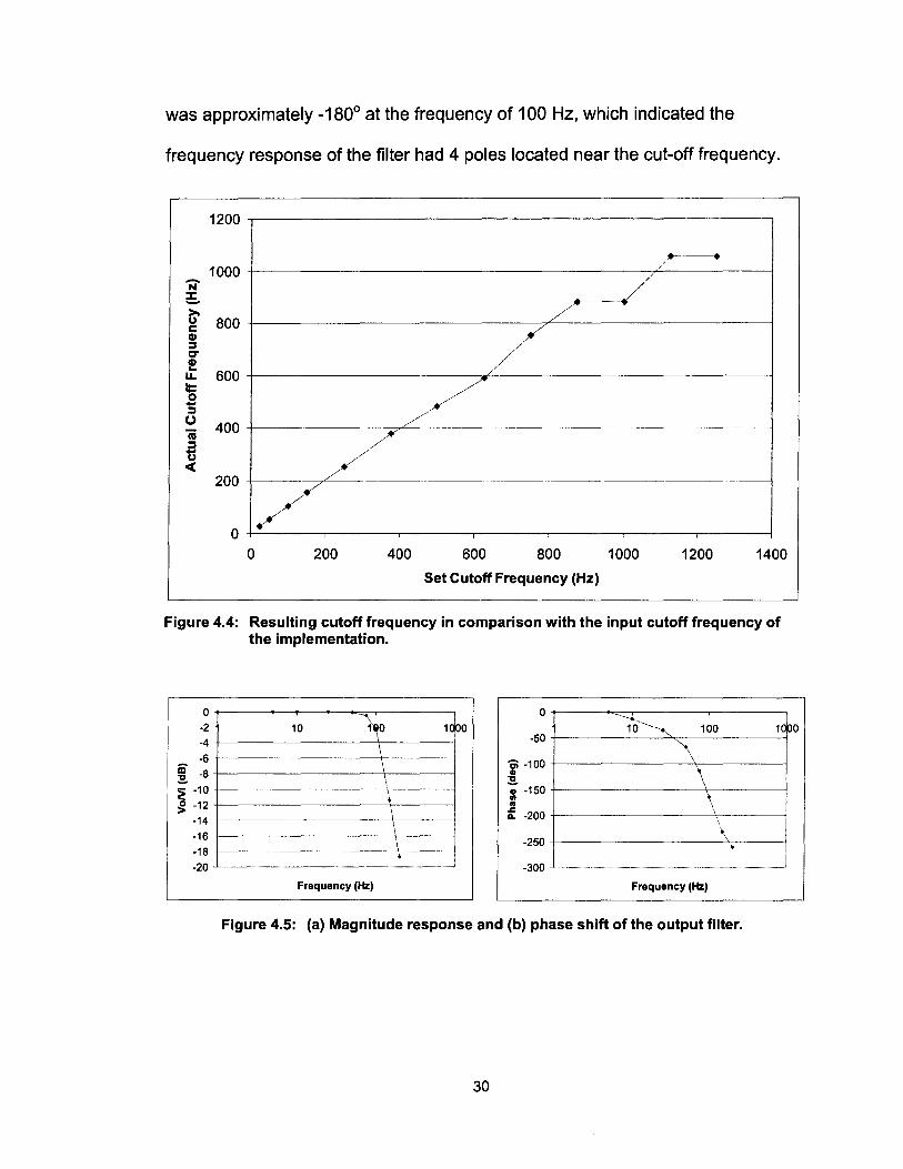
was approximately -180° at the frequency of 100 Hz, which indicated the
frequency response of the filter had 4 poles located near the cut-off frequency.
1200
.-----. 1000 -N
:::E: ->-u 800 c Q) :::I C" f
600 LL ~ .s :::I 0 400 iV :::I 't) c(
200
0
/
~/ //
// /
/ - -//'
// /~
o 200 400 600 800 1000 1200 1400
Set Cutoff Frequency (Hz)
Figure 4.4: Resulting cutoff frequency in comparison with the input cutoff frequency of the implementation.
Or-------~~---=~~------~ -2+-------~'vr-----~im-v----~ -4+--------------\--------1 -6+----------------+-\--~ ! -8+-----------~\~---~
~ -10 • ~ -12+----------+\---~
-14 +--------------+\---~ -16 +-----------+---~ -18 +------------------\---~ -20 ---.-...... -... ---.---------.---.-.... -.. -.--.... ---.-.......... -.... -
Frequency (Hz)
0 0
-50
Ci -100 ... ~ ... -150 1/1
"' it -200 \--250
-300
Frequency (Hz)
Figure 4.5: (a) Magnitude response and (b) phase shift of the output filter.
30
1 0

The attenuation of unwanted high-frequency components present in the
output signal is evident by comparing the unfiltered and filtered output signals
both in time and frequency domains, as shown in Figures 4.6 and 4.7.
~.,..,.....,~p.,....,..rrrI'","",Tri,"g'd:r..-.,....,.... ........ M.;.rPos:.:.: .... o.o:,.;.;,:,OOs"TTTTJ MEASlJlE CH1
~.,..,.....,~p.,....,..rrrI'lI'I'.T.;..;,ri,"9'd:r..-.,....,.... ........ M.;.rPos:.:.: .... O.OO:,.;.;,:,0s"TTTTJ MEASURE CH1
. . . . . . . .. . . . . . . .. ................. . .. ... . .. ... . .. ...
. . .......................................... '" .. . ... . .. . ... . .. ...... . .. ...... . 111111111111111111'11 '.,11111111111111111.11' .. ...... . .. ..... . .. ..... . . .
Pk-Pk 2.84V
CH2 Ott Pk-Pk
elfo Oil fI"'1
· . .. .. ....................... ............ . ... , ....... . · . . . .. . . . . · . . .. .. . · . . .. .. . · -· . . . ................................................ · . .. ... . · . .. .. . · . . . .. . . . . ., ...... .
I I I I I II I I I f I I I II I I I I I I .+, I II I I II I I I I I I I I I I I I I I I · . . . .. . . . . · . . . .. . . . . · . . . .. . . . .
Pk-Pk 2.78\1
CH2 Oft Pk-Pk
! reQ
CH2 Off CH2 Off Freq Freq
CH1 CH1 Freq Freq
, ? , ? C~~~~~~~~~~~~~~2~ C~~~~~~~~~~~~~~~
1 OS. 183Hz 10S.208Hz
(a) (b)
Figure 4.6: (a) Unfiltered and (b) filtered signals at the output (Vpk-pk = 2.78 V, period = 9.7 ms).
Pos: 1.250kHz
-................................... , ........ . .. ...... . .. ...... .
" ...... . .. ...... . . ............ ................................. . .. ...... . " ...... . " ...... . .. ...... . .............................................. · .... .. · .... .. · .... .. · .... ..
I I , I I I I I I I I' I II I I I I I , •• I I I I I I I I I I I I I I I I I I I I I I .. ...... . .. ...... . .. ...... . . .. . . . .
MATH
Operation l1li
Source • Window
lam" FfT Zoom
till Rectangular
103.876Hz
(a)
1.250kHz
-- . . ................. , ......................... . · .. ... . .. . ............................................. .... . .. -.. --. .......................................... . · .. .., . · .. ... . · .. . . · . .., .
I I I II I II I I I I I I I I I I I I'.' I I I I I I I I 'I I I I I I I I I I I · .. .., · .. ... · .. .., · .. ... . . . . . . . .. . . . . . ... .... _ .................... . · .. -' . · .. -' . · .. -' · .. .
MATH
Operation l1li
Source • Window
'1'-'" FFT Zoom
till Rectangular
10S.887Hz
(b)
Figure 4.7: Frequency spectra of (a) unfiltered and (b) filtered signals.
31

5: DESIGN OF ALGORITHM
5.1 Overall Design Structure
The algorithm developed for the design includes the display of a graphic
user interface (GUI), the embedded control algorithm, and the communication
between microcontrollers, as the block diagram of the overall design algorithm
shown in Figure 5.1. On the host PC, a signal-manipulating GUI was designed to
handle the input of signal parameters and the corresponding mathematical
processing. Due to the low priority for the need of continuous and synchronous
data transfer between the GUI and the embedded control, the input signal
parameters are stored in specific sequence in a text file, which can be
subsequently retrieved by the embedded control algorithm. The control algorithm
then encodes the data from the text file to a specific packet format developed to
be transferred to the peripheral over a USB connection. A host interactive
display, which was based on the real-time exchange of data packets between the
host PC and the central control unit, was also programmed to allow real-time
control of the peripheral, including data sending, signal starting and stopping, and
other possible control instructions in further expansion. Upon receiving the data
packets, each of which contains both instruction and coefficient data, the CCU
decodes the instruction and determines what subsequent operation is to be
performed and which signal generating unit (SGU) the instruction is intended for.
32

Graphic User Interface L __ _ '--________ ---'1 File &liVing ----:;:: ___
Host Interactive Display
Embedded Control and Data Encoding / ..,- ::..
------ --------
------ -------------- 1--------, ... 7 ,
CCU Embedded Control , , ,
---l , , , , , ,
, ,
Data Distributing Algorithm Central'
Control Unit , ------ r------------- r--------, ~Z ,
Instruction Decoding Algorithm , , ,
___ --J
---l , , , , , ,
Waveform Generating Algorithm , Signal'
, Generating Unit , _________________ --J
Host
Peripher~1
Figure 5.1: Overall representation of data exchange between interconnected control algorithm blocks
33

5.2 Graphic User Interface
The construction of a simple signal waveform, such as a sinusoidal
function composed of one single frequency component, requires parameters
such as amplitude, frequency, and phase to be defined. A graphic user interface
was developed to handle the input of values and manipulate the desired
waveform using Matlab. Matlab was chosen in this application, owing to its
mathematical processing capability and the GUI programming tool it provided. In
the present application, parameters and coefficients were organized in groups,
each representing the data to be transferred to one single signal-generating unit,
referred to as a channel in this article. These data were stored as comma
separated values in a text file with a specific file name. Once started, the
program loaded the data from the file and stored them in the form of a matrix in
the program memory. Upon the selection of a particular channel, the plotting area
on the GUI displayed the waveform defined by the currently stored values of the
parameters and coefficients associated with the channel. To provide a
mechanism for composing more complex waveforms, the GUI was designed to
handle waveforms of a maximum of five frequency components, each also with a
different amplitude and phase delay. Based on Fourier Theorem, a periodic
signal waveform can be constructed from a series of basic sinusoidal waves of
different frequencies [29]. Since human brainwaves normally consist of only
several frequency components, a mechanism for composing a complex signal
containing a large number of frequency components is not needed in this
application. Furthermore, the cut-off frequency at the output can be arbitrarily
34
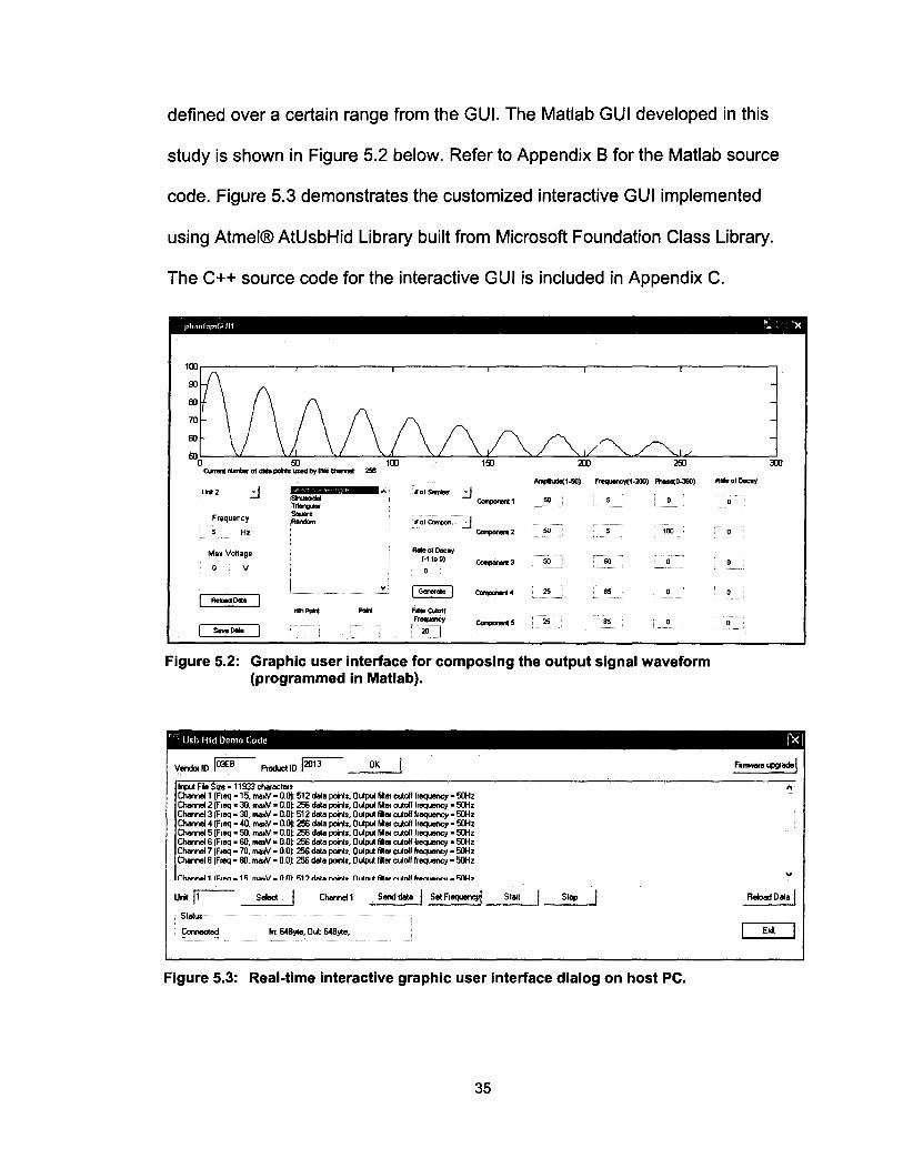
defined over a certain range from the GUI. The Matlab GUI developed in this
study is shown in Figure 5.2 below. Refer to Appendix B for the Matlab source
code. Figure 5.3 demonstrates the customized interactive GUI implemented
using Atmel® AtUsbHid Library built from Microsoft Foundation Class Library.
The C++ source code for the interactive GUI is included in Appendix C.
phanlom(,IJI1 F. I 'X
'-"'2 .:J Frequency
5 Hz
Max VoUago
V
_001.
.. ··9M "i I
:'ofSarries;
;'Of~ ...
_ofOocoy (-I taO)
0 I
I Genor ... I F\lerQAoft Frequency
:~'.~::::.~ ~: .. J
AqlfIude(l-50) Frequeney(1-2OO) 1'tIose(O-36O)
.:J ~1 SO
.:J ~2 SO 1 III
~3 SO SO
~. 2S 65
~5 2S as I 0
Figure 5.2: Graphic user interface for composing the output signal waveform (programmed in Matlab).
:m R'" of Oocoy
"'i( lJ5h Ifid Demo Code rX I
OK Verdot 10 ~ Proc1octlO ~ ----' If1lUI File Size • 11933 character. CMnneI1 (Froq .15, rr.f»N. o..o.~ 512 daI. point., Output filter cutoff frequency. 50iz Chomef 2 (F.oq • 30, rr.f»N • o.o.~ 256 daI. point., Output filter cutoff frequency. 50iz CMnneI3 (F.oq. 30, rr.f»N. o.o.~ 512 daI. point., Output filer cutoff frequency. 50iz CMnneI4 (F.oq • 40, rr.f»N. o..o.~ 256 daI. point., Output filter cutoff frequency. 50iz CMnneI5 (F.oq· 50, rr.f»N • o..o.~ 256 daI. points. Output filter cutoff frequency. 50iz CMnneI6 (F.oq • 60, rr.f»N • o.o.~ 256 daI. point., Output filer cutoff frequency • 50iz CMnneI7 (Freq • 70., rr.f»N • o..o.~ 256 daI. point., Output filter cutoff frequency. 50iz CMnneI8 (F.oq· 80, rr.f»N. o..o.~ 256 daI. point., Output ri .. cutoff frequency. 50iz
u .. r- Select I Stotus
CMnneI1
Comected In 648yte, Out 648)11.,
Send daI. I Set F.equencyl Start Stop
Figure 5.3: Real·time interactive graphic user interface dialog on host PC.
35
RebodDot·1
Ellit
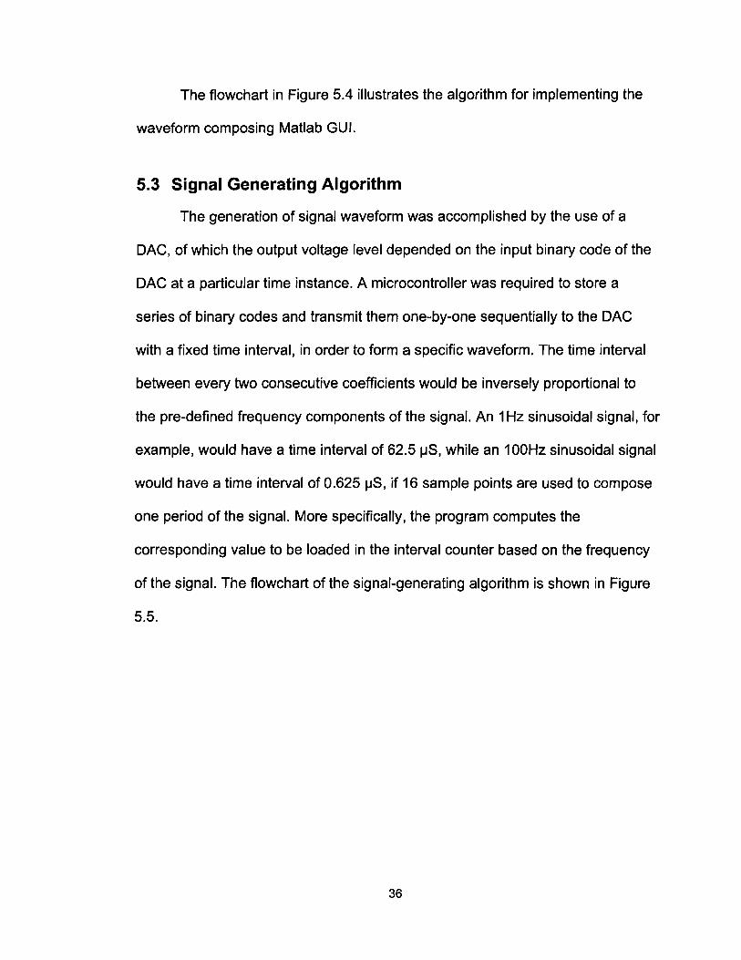
The flowchart in Figure 5.4 illustrates the algorithm for implementing the
waveform composing Matlab GUI.
5.3 Signal Generating Algorithm
The generation of signal waveform was accomplished by the use of a
DAC, of which the output voltage level depended on the input binary code of the
DAC at a particular time instance. A microcontroller was required to store a
series of binary codes and transmit them one-by-one sequentially to the DAC
with a fixed time interval, in order to form a specific waveform. The time interval
between every two consecutive coefficients would be inversely proportional to
the pre-defined frequency components of the signal. An 1 Hz sinusoidal signal, for
example, would have a time interval of 62.5 !-IS, while an 100Hz sinusoidal signal
would have a time interval of 0.625 !-IS, if 16 sample points are used to compose
one period of the signal. More specifically, the program computes the
corresponding value to be loaded in the interval counter based on the frequency
of the signal. The flowchart of the signal-generating algorithm is shown in Figure
5.5.
36

No
Ol)en GUI
Instantiate GUI components
Load the parameter
containing text file
Perform corresponding
functions
Store change in data for the
particular channel
Save paramters to the text file
Close GUI
Figure 5.4: Control algorithm of the Matlab GUion host PC.
37

Start
Interval calculation based on frequency
Load DAC with a starting pulse
8et up counters for coefficient count and
Interval
Reset Index pOinter
Yes Load DAC with
No
Load DAC with the next coefficient
Decrement interval counter
Decrement coefficient counterl Increment Index pOinter
No Yes
zero
Figure 5.5: Implementation of the signal generating algorithm of SGU.
38
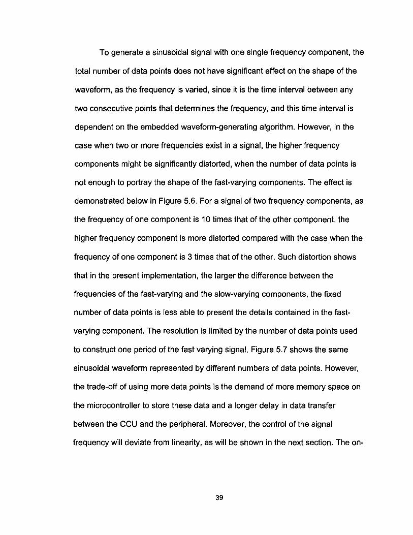
To generate a sinusoidal signal with one single frequency component, the
total number of data points does not have significant effect on the shape of the
waveform, as the frequency is varied, since it is the time interval between any
two consecutive points that determines the frequency, and this time interval is
dependent on the embedded waveform-generating algorithm. However, in the
case when two or more frequencies exist in a signal, the higher frequency
components might be significantly distorted, when the number of data points is
not enough to portray the shape of the fast-varying components. The effect is
demonstrated below in Figure 5.6. For a signal of two frequency components, as
the frequency of one component is 10 times that of the other component, the
higher frequency component is more distorted compared with the case when the
frequency of one component is 3 times that of the other. Such distortion shows
that in the present implementation, the larger the difference between the
frequencies of the fast-varying and the slow-varying components, the fixed
number of data points is less able to present the details contained in the fast
varying component. The resolution is limited by the number of data points used
to construct one period of the fast varying signal. Figure 5.7 shows the same
sinusoidal waveform represented by different numbers of data points. However,
the trade-off of using more data points is the demand of more memory space on
the microcontroller to store these data and a longer delay in data transfer
between the CCU and the peripheral. Moreover, the control of the signal
frequency will deviate from linearity, as will be shown in the next section. The on-
39

chip EEPROM of the ATMega32 microcontroller used for storing the data points
in the implementation allows a maximum of 1024 data points.
p \ I \ . \
. \ '\
\
(a) (b)
Figure 5.6: Representation of a sinusoidal signal (a) 3 times and (b) 10 times of the coexisting fundamental frequency, both with 32 quantization coefficients.
250
100
50
-16 coefficients - - -64 coefficien1s _. _. -512 coefficients ........ -1024 coefficients
Figure 5.7: A sinusoidal signal composed of different numbers of quantization coefficients.
Another advantage of representing a signal with a larger number of data
points is the reduction of high-frequency components of the signal generated,
40

which usually consist of unwanted noise. Such effect can also be illustrated in the
frequency domain. Figure 5.8 below shows the frequency responses of an 100-
Hz sinusoidal signal, constructed using different numbers of data points. It can be
observed that as the number of data points representing a single period
increases, the number and magnitude of higher-frequency spikes are reduced.
However, representing a signal waveform with a larger number of quantization
coefficients using the present signal generating method is not without its trade-
off, as will be explained in the next section.
MATH
Operation l1li
· , ... .................................................. · . . . .. . . . . · ..., . · . . . .. . . . . · . . . .. . . . . · ................................................ . · . . . .. . . . . Sowce · . . .., .. · . . . .. .. . · . . . .. . . . . IIiiI · ......................... , ...................... . · . . . .. . . . . · . . . .. . . . . · . . . .. . . . . · . . . .. . . . . 111111111111111111111111.,11111111111111111111111 · . . . .. . . . . · . . . .. . . . . · . . . .. . . . . · . . . .. . . . . · ............................................... .
Window · . . . .. . . . . · . . . .. . . . . · .. : ... : ... : ......... : ... : .... : .... : .... : .... '@I-'" · ., ..... . · .. ..... . .. . . .
Rectangular 102.377Hz
(a)
Tek JL Pos: 12050kHz MATH
Operation l1li
· . .. . .................................................. · . . . .. . . . . · . . . .. . . . . · . . . .. . . . . · . . . .. . . . . · ......................... ' ...................... . · . . . .. . . . . Source · . . . .. . . . . · . . . .. .. . IIiiI · . .. ... . · ......................... , ...................... . · . . . .. . . . . · . . . .. . . . . · . . . .. .. . · . . . .., .. , • I I I • I •• I • 1,1' , ,. I I I • I I.' I I I ,. I II , •• , I • I II •• , I I I · '" . . ... . . . . . ... . . · ......................... , ...................... .
Window · . . . .. . . . . · .... . ... ~ .... ~ .... ~ .... ~ .... ~ .... ~ .... ~ .... ~ .... ~ .... 'MD'"
· . . . .. . . . . . - . .' ... : ........ : .... : ... : .... : .... : .... : .... FFTZoom
· :::::: II
(c)
Rectangular 101.328Hz
Tek JL Pos: 12050kHz MATH
Operation l1li
· .. .. . · ................................. , .............. . · . . . .. . . . . · .. .... . , .. ..... . · .. .. .................................................. · . . . .. . . . , Source · . . . .. . . . . · . . .. . . . · . . . ... . . . . IIiiI . ....................... " .... , ........... , ...... . · . . . .. . . . . · . . . .. . . . · . . . .. . . . · . . .. . . . .
I I I • I • " I • I. " , II I I • I I , •• , I • I I I I , , I I • , , • I I I I , I I • , · . . . .. . . . . · . . . .. . . . . · . . . .. . . . . · . · . . .. Window
· .. : .... ~ ... ~ .... ~ .... ~ .... ~ .... ~ .... ~ .... ~ .... 'MD'" · . . .. . . . · . ... .
Rectan9ular 1020288Hz
(b)
Tek JL Pos: 12050kHz MATH
Operation l1li
· . .. '" . ................................................ . · . . . .. . . . . · . . . .. . . . . · . . . .. . . . . · . . . .. .. . . ................................................ . · . . . .. . . . Source · . . . .. . . . · . . . .. . . . · . . . .. . . . IIiiI · ................................................ . · . . . .. . . . . · . . . .. . . . . · . . . .. . . . . ., . I I II I I I 1'1' II I I I I " I I I I ••• I I I , I I I I 1 I I I 'I I • I I I I , I I · . . . .. . . · . . . .. . . · . . . .. . . · . . . .. . . · ................................................ . · . . . .. . . . . . ..... . Window · .. ~ .... ~ .... ~ .... ~ .... ~ .... ~ .. " ~ .... ~ .... ~ .... 'aD'"
· . . . .. ., . · . . . .. . . · . .
(d)
FFT Zoom II
Rectangular 1020579Hz
Figure 5.8: Frequency spectra of an unfiltered sinusoidal signal of 100Hz fundamental frequency formed with (a) 32, (b) 64, (c) 128, and (d) 256 quantization coefficients
41

5.4 Frequency Calibration
As mentioned previously, the frequency of a generated waveform is
controlled by adjusting the length of interval between consecutive voltage points.
The frequencies of produced waveforms, therefore, need to be calibrated against
the desired frequency of the signal. To accomplish this, a sinusoidal signal with a
single desired frequency is defined and compared with the actual signal
waveform generated. Figure 5.9 shows that the relationship between the
resulting frequency and the value set from the GUI when different numbers of
data points are used to compose a single period of the waveform. It can be
observed that with the current waveform-generating algorithm, the output
frequency levels off at high frequency region. Furthermore, as more data points
are used to compose a period, the actual output frequency levels off at a lower
value.
42

400
350
300
~ 250 ~ I: CD ::;, 200 ~
u.. ii ::;,
150
~ 100
50
0 0 50 100 150 200
Set Frequency (Hz)
250 300
---+-32DP
• 64DP
• 128DP
--)(--256DP
--*-512DP
Figure 5.9: Relationship between resulting frequency of the output sinusoidal signal and the input value of frequency for different number of quantization coefficients before frequency calibration.
The lower-frequency regions of the curves exhibit more linearity between
the output frequency and the set value and thus can provide more linear control
of the desired signal frequency. Therefore, it is of great interest to adapt the
waveform-generating algorithm to the more linear low-frequency regions. By
increasing the length of interval between consecutive output data points, the
lower-frequency regions of the curves can be extracted to span the input value
range. This was accomplished by doubling the initial count of the counter for
controlling the interval between consecutive points. However, the output
frequency range is only limited to the lower half of the curves shown. By setting
the system clock of the microcontroller to a higher speed, the resulting output
frequency can be increased. Figure 5.10 below shows the resulting relationship
43

as the length between the data points was doubled, while the system clock was
increased from the original 1 MHz to 4 MHz. It can be observed that with the
same operating conditions, the resulting output frequency exhibited a larger
degree of linearity over the desired range.
350
300 /,/
~ 250 ~/
::::./ ~ 32 DP ~
/ //--- • /' /' c 200 .-~/¥ _64DP Q) :::J ~~/ , ____ ---X g-
" 128 DP I!! / X-----II. 150 ~ .~ ----/- -K-256 DP iii /;////X---
512 DP :::J g~~---.--)I(-----------)I( :t:: :i 100 g)(/ ~-----
/ -----------
50 /~--0
0 50 100 150 200 250 300 Set Frequency (Hz)
Figure 5.10: Relationship between resulting frequency of the output sinusoidal signal and the input value of frequency after frequency calibration.
5.5 Embedded Control and Communication
The communication between the host computer and the CCU and
between the CCU and any of the SGU is accomplished by the exchange of data
packets having data bytes in a specific sequence. These data packets are
constructed using a format similar to the format in computer networking
protocols, by appending bytes that indicate the command to be executed and
relevant parameters to coefficient bytes. Initially, for each single channel, the GUI
saves the data in the format shown in Figure 5.11 below, as an array of
44

parameters followed by the coefficients for constructing a period of signal. The
CSV file generated by the GUI contains arrays in such a format, while the
number of arrays in the file depends on the total number of SGU attached to the
CCU. Once the host interactive display is launched, the embedded control
algorithm on the host PC loads the content of the CSV file into its program
memory. Every time a function call is made on the host interactive display, one or
more packets would be sent to the CCU via the USB connection, including a pilot
packet (Packet 1) containing the instruction byte. If the instruction byte in the pilot
packet is for coefficient transfer, the number of data packets sent depends on the
total number of coefficients (data points) used for constructing a particular
waveform. Upon receiving the pilot packet, the microcontroller on the CCU reads
byte 6 of the pilot packet that indicates the total number of data points as a
multiple of 32 and determines the total number of data packets to be received
following the pilot packet. With this implementation, the total number of data
points is no longer limited to the maximum number of bytes that can be sent in
one single packet, as the USB communication protocol provided by Atmel® limits
the maximum number of bytes in a packet to 64 bytes. Figure 5.12 shows the
structure of packets sent to the CCU by the host PC for each data transfer. In the
pilot packet, depending on the command to be executed, the corresponding
instruction byte following the channel 10 of the intended unit is attached to the
front of an array containing various signal parameters, such as the base
frequency, max voltage, and etc .. Upon receiving these data packets, the CCU
initiates an external interrupt on the intended SGU, and the data are re-directed
45

to the intended channel via the demultiplexing circuit. The source code of the
CCU embedded algorithm is included in Appendix o. While the microcontroller
on each SGU is pre-programmed with an unique channel 10, the addition of
channel 10 byte to the packet to be sent can prevent any unintended SGU to
execute the command. For example, if a propagation delay caused by the
demultiplexing network results in the data packets being routed to an unintended
channel, the SGU at the receiving end would discard the packets because the
channel 10 in the pilot packet does not match the pre-programmed 10 of the
receiving SGU. In the present design, the packet can easily accommodate up to
256 channels and 256 different function calls.
Figure 5.11: Data structure of the stored parameters for each individual channel on host PC.
Figure 5.12: Structure of the packets sentfrom host PC to CCU during each data transfer.
46

No
No
Start
Initialization of the microcontroller
Channel numbe decoding
Instruction decoding
No
Sending the next coefficient to DAC
No
Figure 5.13: Command-decoding algorithm on each SGU.
47

The command decoding sequence implemented on each SGU
microcontroller is illustrated in Figure 5.13. Once the SGU microcontroller
receives the pilot packet, and the instruction is decoded to be coefficient transfer,
byte-by-byte data transfer is performed between the CCU and the intended SGU.
The scheme of coefficient transfer implemented is shown in Figure 5.14. The
communication between the CCU and the SGU consists of four states, dictated
by CommO and Comm1 signal lines. The CommO and Comm1 were
implemented using a pair of I/O ports between the CCU microcontroller and the
SGU microcontroller. CommO signal line was configured as an output for the
CCU and an input for the SGU. The direction of the Comm1 line was the inverse
of that of CommO. Another connected I/O port between the CCU and the SGU
was used for transferring the byte data, with the CCU being the sender and the
SGU being the receiver. Upon the start of transfer, both CommO and Comm1
lines are reset to '0', and the system is in Reset state. After the CCU writes the
new byte of coefficient to the data port, it sets CommO to '1' to indicate a new
byte is ready for the SGU to receive. The system is in Data Ready state at this
stage. The SGU then reads the new byte of data from the data port and set
Comm1 to '1'. The Data Received state indicates to the CCU that the current
byte has been received and a new byte of coefficient can be written to the data
port. Once the CCU detects a '1' on Comm1, it resets CommO to '0' to switch to
Cycle Complete state. Subsequently, the SGU resets CommO to '0', and the
entire cycle is repeated for each of the coefficients. The end of transfer is done
by exiting the loop when all the coefficient bytes are finished transferring. The
48

communication is achieved by the CCU controlling the status of CommO line and
the SGU controlling the status of Comm1 line. In any of the states, both the CCU
and the SGU should check the status of both the CommO and the Comm1 lines
and perform the corresponding tasks before altering its own signal line. Refer to
Appendix E for the detailed control algorithm for each SGU microcontroller.
~ sou resets Comm1
Cycle Complete CommO= '0' Comm1 = '1'
Reset CommO= '0' Comm1 = '0'
Data Received CommO= '1' Comm1 = '1'
CCU writes to the data port, setting CommO to '1 '
~
Data Re.ldy CommO= '1' Comm1 = '0'
sou reads from the data port, setting Comm1 to '1 '
Figure 5.14: Communication states of data point forwarding from CCU to SGU.
49

6: MEASUREMENT AND ANALYSIS
6.1 Experiment and Method
A more delicate method of positioning coils was devised, which allowed
more coils to be mounted on a head-shaped object simultaneously. Each coil at
the end of a twisted pair was firmly glued on a flat wooden stick with markings
indicating every centimetre, as illustrated in Figure 6.1. These markings were
later used for determining the relative spatial coordinate of the coils with respect
to the reference points in the Polhemus measurement system.
Figure 6.1: (a) A helical coil (3 loops) and (b) an isosceles triangular coil fixed on a wooden stick. The distance between two adjacent marked lines on the stick is 1 cm.
These sticks were then mounted on a plastic skull fixed on the base, as
shown in Figure 6.2 below. Holes were drilled at spots evenly distributed on the
plastic skull. Then a sheet of rubber layer was glued on the surface of the skull.
Holes were opened on the rubber sheet at the corresponding locations. Then
these sticks with the coils attached were inserted into the holes on the skull and
50

held in place by the rubber sheet. Three reference coils (not shown in Figure 6.2)
which define the nasion, left ear, and right ear positions were fixed on the base
instead of the corresponding positions on the plastic skull. The reference coils
also emitted signals recorded by the MEG system; these signals were used for
determining the relative location and orientation of the test subject in the
measurement cavity. The overall control and signal generating electronics used
in the experiment is shown in Figure 6.3.
Figure 6.2: (a) Front view, (b) left-side view, and (c) right-side view of coil placements on a plastic skull covered with a layer of rubber sheet mounted on a plastic base.
51
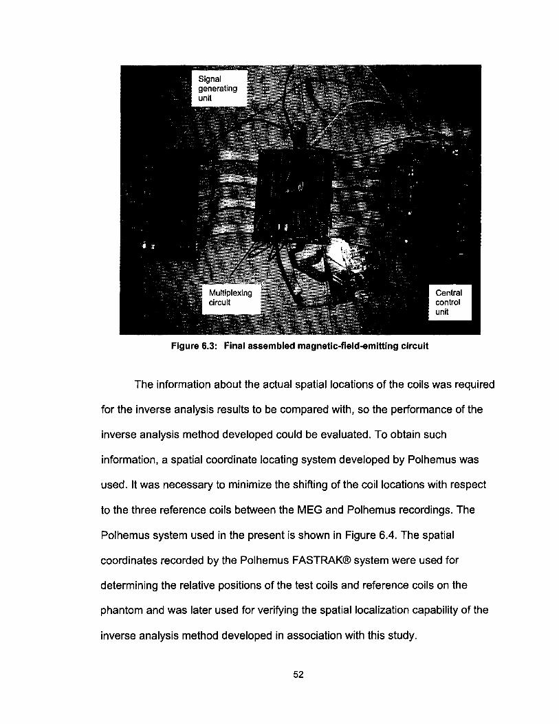
Figure 6.3: Final assembled magnetic-field-emitting circuit
The information about the actual spatial locations of the coils was required
for the inverse analysis results to be compared with, so the performance of the
inverse analysis method developed could be evaluated. To obtain such
information, a spatial coordinate locating system developed by Polhemus was
used. It was necessary to minimize the shifting of the coil locations with respect
to the three reference coils between the MEG and Polhemus recordings. The
Polhemus system used in the present is shown in Figure 6.4. The spatial
coordinates recorded by the Polhemus FASTRAK® system were used for
determining the relative positions of the test coils and reference coils on the
phantom and was later used for verifying the spatial localization capability of the
inverse analysis method developed in association with this study.
52

Figure 6.4: Polhemus FASTRAK® 3D Digitizer used for localizing points in 3D space, including a transmitter and a receiver fixed around the test skull during the experiment and a stylus used for physically locating the coils on the skull.
6.2 MEG Measurement using Helical Coils
Measurement was taken using helical coils mounted on the surface of the
plastic skull with relative locations of which the planar view is illustrated in Figure
6.5. All coils were wound with the best attempt to keep the geometry the same.
6
3 2
~ 1
Figure 6.5: Relative locations of the helical coils on the head surface.
53

.ro .
100
50 .. (a)
°O~""--------~50~~----------~I~oo------------~I50 FreqJerof [Hz)
(b)
FreqJerof [Hz)
Figure 6.6: Frequency spectra of (a) all coils at 13 Hz, maximum current and (b) all coils at 13 Hz, minimum current.
The frequency spectra of measured magnetic flux density under various
test conditions are shown in Figures 6.6 and 6.7. It can be observed all the
intended frequency components were visible in the recorded magnetic fields.
Notably the signal at 60 Hz was likely due to the noise present in the power
supply.
54
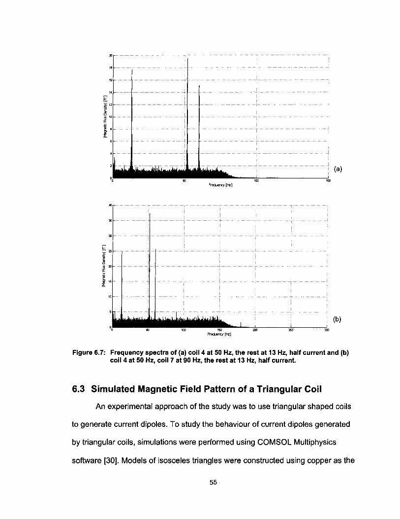
20·
(a)
freQ-JErcy [Hz)
36·
30
(b)
Figure 6.7: Frequency spectra of (a) coil 4 at 50 Hz, the rest at 13 Hz, half current and (b) coil 4 at 50 Hz, coil 7 at 90 Hz, the rest at 13 Hz, half current.
6.3 Simulated Magnetic Field Pattern of a Triangular Coil
An experimental approach of the study was to use triangular shaped coils
to generate current dipoles. To study the behaviour of current dipoles generated
by triangular coils, simulations were performed using COMSOL Multiphysics
software [30]. Models of isosceles triangles were constructed using copper as the
55

material, as illustrated in Figure 6.8. Each side of the triangle consisted of a long
cylindrical shape with a diameter of 0.15 mm. Since the wire had a constant
resistance, the current in the coil was proportional to the applied voltage. The
current density through any cross sections along the long axis of all three
cylinders would be constant. Notably the corner effect of the triangular shape
was neglected in the simulation models constructed. Nonetheless, the relatively
small thickness of the wire compared to the dimensions of the triangular shapes
simulated, the corner effect would not result in significant difference between the
simulated and actual magnetic fields.
Base
Figure 6.8: Example triangular coil model constructed in COMSOL.
The orientation of the coil in the simulated space is shown in Figure 6.9
below. The coils were oriented with the base side of the triangle parallel to the x
axis at z = 0 of the simulated space.
56

Figure 6.9: Simulated space in COMSOl, consisting of a cube of 10-cm side length.
It was of interest to investigate on the magnetic flux density generated by
the coil in each dimension of the simulated space. The patterns of the axial
components of magnetic flux density in the xy, yz, zx planes 5 cm from the origin
are shown in Figure 6.10, respectively. By varying the leg length of the triangular
coil while keeping the base length constant at 5 mm, the magnetic flux density
normal to any plane in the simulated space can be compared. Since
magnetoencephalography detects only the tangential component of the source
current, it is of interest to monitor z-component of the magnetic flux density in the
xy-plane, which is parallel to the base side of the triangular coil.
57
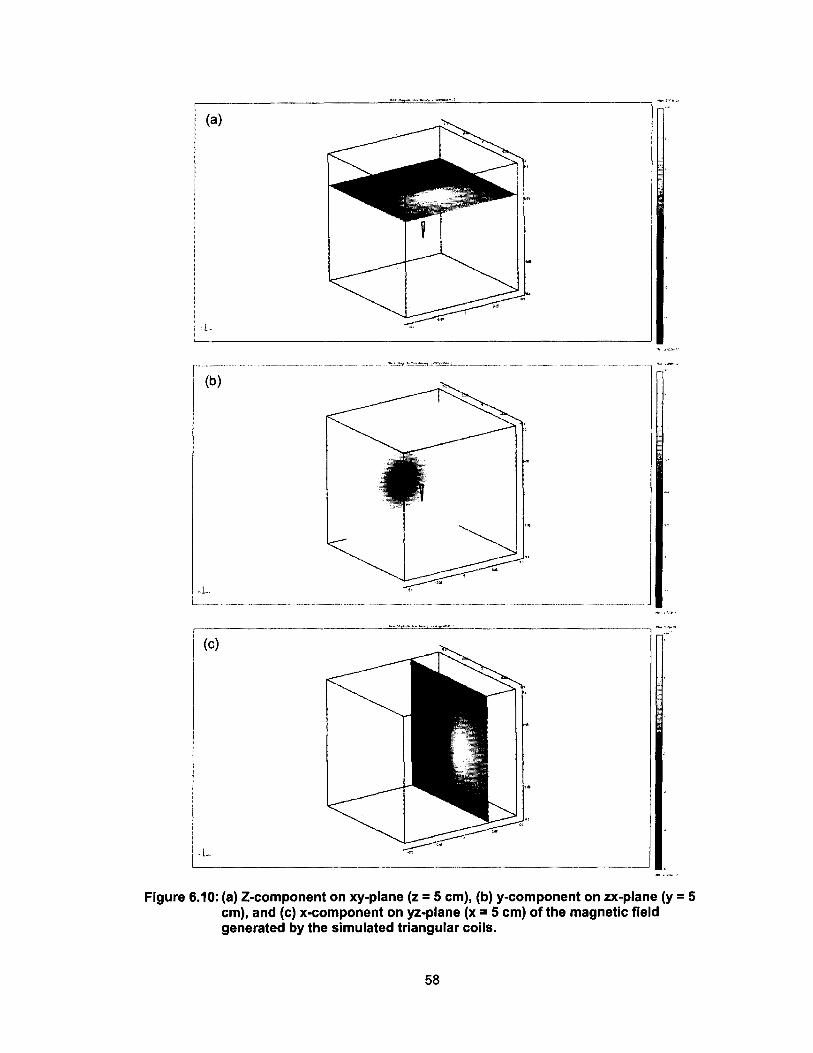
,---___________ "'..:""=.!::.~,""_'_ ______________ '-"'IIO,{
,t,"
(a)
(c)
Figure 6.10: (a) Z-component on xy-plane (z = 5 cm). (b) y-component on zx-plane (y = 5 cm). and (c) x-component on yz-plane (x = 5 cm) of the magnetic field generated by the simulated triangular coils.
58

Simulation results indicated the locations of maximum z-component of the
magnetic flux density on a given xy-plane remained unchanged irrespective to
the change of base and leg lengths, as long as the origin was fixed at the center
of the base (See Appendix F). Nonetheless, the maximum y-component on any
given zx-plane varied as the geometry of the triangle was changed. It appeared
to be located at the same x and z coordinates as the triangle's centroid.
The maximum z-component magnetic flux density normal to the xy-plane
at z = 5 cm, and the y-component along the y-axis on the zx-plane at y = 5 cm for
various leg-to-base ratios of the coil are shown in Figures 6.11 and 6.12,
respectively, while the base was kept constant at 5 mm.
1.40E-11
1.20E-11
'iii 1.00E-ll iii
~ > ... 'iii 8.00E-12 c QI '0 )( :J
;;: 6.00E-12 u ..
QI C l1li AI
:E 4.00E-12
2.00E-12
O.OOE+OO
0 5 10 15 20
Leg/Base ratio
25
-+-2mm base ___ 5mm base
" 10mm base
Figure 6.11: Max z-component magnetic flux density in the xy-plane at z = 5 cm from origin of isosceles triangular coils.
59

4.00E-ll
3.50E-ll
'iii' 3.00E-ll
~
~ > 2.50E-ll : ... 'in c CII ~
2.00E-ll >c ::l Ii: u .. CII 1.50E-ll c 110 III
:IE 1.00E-ll
5.00E-12
O.OOE+OO
0
,
i
5 10 15
Leg/Base ratio
20 25
-+-2mmbase ___ 5mm base
.~ 10mm base
Figure 6.12: V-component magnetic flux density in the zx-plane at y = 5 cm (x = 0, Z = 0) from origin of isosceles triangular coils
The simulated magnetic flux densities appeared to level off at different
values of leg-to-base ratio, when the base length was varied, for both z- and y-
components. Next, the effect of increasing the length of the base side of the coil
was to be modeled. By constructing an equilateral triangular coil with various side
lengths, the magnetic flux density normal to the planes at the same above
mentioned positions in the simulated space was modeled, as shown in Figure
6.13 below.
60

1.20E-10 --------------------,
1.00E-10
-~ 11\
~ B.00E-11
> ... 'iii c QI
"tJ 6.00E-ll )( -.- z-component :::J
;:;:::: ......... v-component u
'';:; QI c 4.00E-ll bO IV
~
2.00E-ll
O.OOE+OO
o 5 10 15 20 25 30 35 40 45
Side length (mm)
Figure 6.13: Max magnetic flux density in the plane perpendicular to the axial component at 5 cm from origin of equilateral triangular coils.
The simulation result indicated that as the leg-to-base ratio increased, the
y-component of the resulting magnetic field at the vicinity of the origin behaved
more similarly to a current dipole.
6.4 MEG Measurement using Triangular Coils
MEG data were recorded using triangular coils mounted on the plastic
skull, as mentioned in the method above. The relative locations of the coils on
the test skull are illustrated in Figure 6.14 below. Table 6.1 shows the measured
dimensions of different triangular coils tested.
61
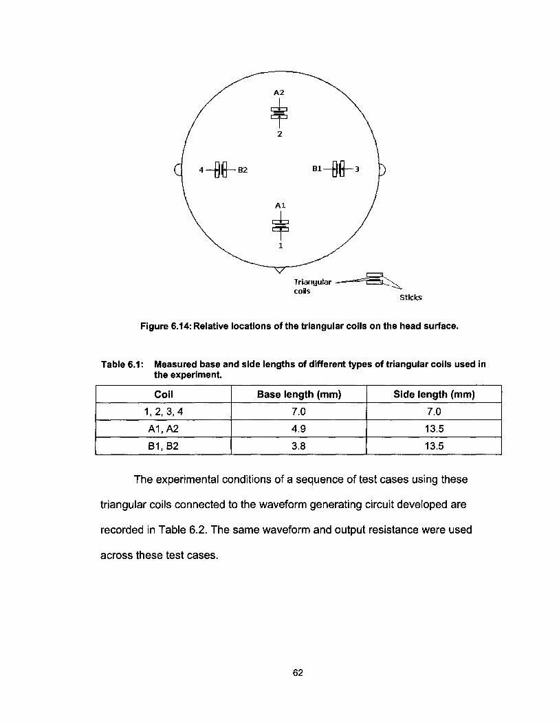
4-9&-82
A2
~ ~
2
A1
~ ~
1
81-9&-3
Triangular ~5~ coils
Sticks
Figure 6.14: Relative locations of the triangular coils on the head surface.
Table 6.1: Measured base and side lengths of different types of triangular coils used in the experiment.
Coil Base length (mm) Side length (mm)
1,2,3,4 7.0 7.0
A1,A2 4.9 13.5
81,82 3.8 13.5
The experimental conditions of a sequence of test cases using these
triangular coils connected to the waveform generating circuit developed are
recorded in Table 6.2. The same waveform and output resistance were used
across these test cases.
62

Table 6.2: Coils energized in different test cases in the experiment.
Test case Coils energized
1 1
2 A1
3 2
4 A2
5 1,2
6 A1,A2
7 3,4
8 81,82
9 1,2,3,4
10 A1, 81, 82
11 1,2,3,4,A1,A2,81,82
The actual locations of the MEG sensors are evenly distributed around the
measured space, illustrated in Figure 6.15. Each channel consists of an inner
sensor and an outer sensor.
.0.3
025
0.2
'E 0.15 ..... N 0.1
0.05
o
Sensors
x em) y [m}
Figure 6.15: Spatial distribution of sensors around the measured space, for a total of 151 channels, each having an inner and an outer sensors.
63

The spatial distribution maps of measured magnetic fields at a particular
time instance for different test cases are shown in Figure 6.16 below. In this
case, time was equal to 1.1 seconds since the beginning of recording. The
artifact of using a triangular coil to simulate a current dipole can be observed
towards the back of the measuring space, as sensors were located more towards
the posterior of the measuring cavity to cover the surface of occipital cortex. As
indicated by COMSOL simulation in the previous section, a triangular coil
produces a magnetic field, the pattern of which contains the characteristics of
both a magnetic dipole and a current dipole.
4(0) DlJ
DlJ :1OOJ
:1OOJ
1(0) 1(0)
0
.1(0) .1(0)
.:1OOJ .:1OOJ
·DlJ
.4(0) ·DlJ
Test case 1 Test case 2
5IID 1500
4(0)
1(0) DlJ
:1OOJ 500
liD)
0
·1(DJ -500
.:1OOJ
.1(0) ·DlJ
.4(0)
·1500 -5000
Test case 5 Test case 11
Figure 6.16: Spatial magnetic flux density distribution of test cases 1, 2, 5, 11 at time equal to 1.1 seconds after the start of recording (Unit: fT).
64

Time-line Data Time-line Data 500J
400:)
DlJ
~ ~ >- >-1ll .~
Ii ~ 0 0 M 11 .2 IL IL
." 10 §,
~
-4OJJ .400:)
0.6 0.7 O.B 0.9 1 1.1 1.2 1. .6OJl 0.6 0.7 O.B 0.9 1 1.1 1.2 1.3 1.4 1.5 1.6
TIme lsI TIme lsi
Test case 1 Test case 2
1 .104 Time-line Data Time-line Data
fOlJ
O.B 6000
0.6
~
£
TIme lsi TIme lsi
Test case 7 Test case 8
Time-line Data Time-line Data
0.6 0.7 O.B 0.9 1 1.1 1.2 1.3 1.4 1.5 1.6 TIme 1'1
0.6 0.7 O.B 0.9 1 1.1 1.2 1.3 1.4 1.5 1.6 TIme 1.1
Test case 10 Test case 11
Figure 6.17: AC component of the recorded magnetic flux densities on all channels for test cases 1, 2, 7, 8, 10, and 11.
The AC components of the measured magnetic flux density with respect to
time at different channels are shown in Figure 6.17 above. Excluding the DC
65

component allows the signals emitted by different sources to be more
distinguishable.
Comparing the AC component of experimental magnetic flux density
across test cases 1 and 2, 3 and 4, 7 and 8 reveals consistency between the
simulated and experimental data of change in magnetic flux density with respect
to the geometry change of the triangular coil. The increase in the recorded
magnetic field complexity is observable, as the number of magnetic field sources
increases. Also noticeable in the figure is the opposite magnetic field associated
with the induced current on the other coil when only one single coil was
energized, due to the arranged proximity in locations for each pair of coils. The
resulting magnetic flux density and locations of dipoles obtained from each of the
TSVD, data clustering, and downhill simplex computation inverse analysis steps
for several experimental trials are illustrated sequentially in Figure 6.18 (See
Appendix G for the inverse analysis results of the other test cases). The actual
locations of the dipoles derived from the Polhemus measurement are also shown
in the figure. It can be observed that the inversely mapped dipole locations
converged more toward the actual locations after each subsequent step.
66

.. ...
:J U, . -a, ....
..
_ ......
1SVD"""
,Dfjllila ~ A/,/ SiIaO
1IW_
.. la' I': . ...
"'1 _" .... 00 o ...
"
.. ...
:J" .
... "
--o
Test case 5
.. ."
-0, .. .... 00
• iIiIII .,
o
O<ii<liIa ~ A/,/ lilaO
Obnlr ........ ~
.. "" ..
~ lu, .~ .. -a-
0
-0' .., .... CD
• iIiIII
III .r..J
Test case 9
--.. "t ~ .
lin .~ ... 0 ..., q, ....
" ... U
,",W
--.. .,.
:ill
-0, .. .... 00
0 ... ., 'flo! ,r..J
Dfjllila~A/'/lila0 _ ......
.. ... i'-< :J .. ..
0
-0, .., .... m 0 ...
,r..J
Figure 6.18: Left - Resulting magnetic flux density distribution after TSVD; middleResulting dipole locations after data clustering; right - Adjusted dipole locations after downhill simplex computation of test cases 5, 8, and 9.
The resulting dipole moments from inverse analysis for different test cases
are listed in Table 6.3. The results were grouped into dipole numbers according
to their associated coils. The orthogonality for each dipole across different test
cases was also calculated. As shown by the table, the directionality of each
individual inversely mapped dipole moment was fairly consistent across different
67

test cases. However, the analysis result exhibited a large variation in terms of the
magnitude for the same dipole across different cases.
Table 6.3: Resulting dipole moments for the dipole associated with each coil across different test cases from the inverse analysis and their correlation.
Dipole moment (nA o m2) Orthogonality
Dipole Test With case x-comp y-comp z-comp Magnitude test [a·b]/[lallbl]
case
1 -11.4126 -2.64473 4.2279 12.4546045 5 -0.99712
1 5 4.44082 0.694774 -1.79769 4.84100016 8 -0.99722
8 -9.07006 -2.16781 3.86496 10.0947167 1 0.998896
3 9.08655 0.745644 4.78266 10.2953976 5 0.989986
2 5 4.00989 0.247444 2.89069 4.94939744 8 0.968141
8 2.25881 -0.25313 1.01386 2.48881679 3 0.982892
2 9.99079 1.81074 -3.97841 10.9051552 6 0.997893
A1 6 13.8897 2.01862 -6.43405 15.4400645 9 0.996194
9 12.0714 2.11669 -4.43003 13.031663 2 0.999632
4 -15.3359 2.13292 -7.68465 17.2856305 6 -0.98913 A2
6 11.8206 -2.03927 8.30499 14.5896561 - -
7 -3.46474 4.62228 5.79692 8.18377524 9 -0.9823 B1
9 3.66125 -6.27462 -5.18878 8.92743219 - -
7 -0.54642 7.23373 -7.91303 10.7350581 9 0.998203 B2
9 -0.25029 2.21183 -2.17895 3.11490925 - -
3 8 4.06249 -8.84695 -8.80414 13.1257469 - -
4 8 0.485255 -5.99561 6.46891 8.83343695 - -
68

7: CONCLUSION AND FUTURE WORK
7.1 Conclusion
Cognitive science and brain clinical research can benefit from MEG,
provided that a reliable inverse analysis technique for localizing the active
regions in the brain can be developed. A consistent electronic method was
devised to provide the ground truth for the verification of a novel inverse analysis
technique developed by attempting to physically simulate the magnetic fields
emitted by active brain neurons. Moreover, the feasibility of using triangular coils
to simulate current dipoles, which more faithfully represent neuronal activities,
was also studied. Both simulation and experiment revealed that triangular coils
with finite base lengths still produce magnetic field patterns of magnetic dipoles.
Another drawback of using coils for emitting magnetic signal observed is the
undesirable induction across coils of close spatial proximity. The inverse analysis
method developed in association with the present study provided accurate
estimate of the actual dipole location and directionality, while the consistency for
estimating the dipole magnitude requires improvement.
7.2 Future Work
Using the signal generating mechanism developed in the present study, a
more complex combination of signals across different sources can be devised in
the next phase of inverse analysis method development. Moreover, the use of
triangular coils with finite base lengths still does not truly simulate a current
69

dipole, which can more realistically model the ion exchange process in a cluster
of active brain neuron than a magnetic dipole. A more sophisticated approach
might involve the use of capacitive elements in the circuit to store charges until a
controlled triggering event. How to avoid the interference of the generated signal
due to the triggering mechanism is also subject to further study. In the electronics
aspect, the method for emitting magnetic signal in the present study does not
allow controllable synchronization of signals across different signal generating
units. Having more synchronized signal across different sources might post more
challenge to the inverse analysis. The future aim is to allow the signal pattern
resulting from the MEG recording of human subjects to be replicated on the
signal-generating device before the spatial mapping of sources can be
proceeded. A more finely calibrated spatial fixation of the coils is also subject to
more development for any clinical purposes.
70

APPENDICES
71

Appendix A: Schematic Drawings
Appendix A 1: Schematic of standalone waveform-generating unit in previous implementation
I. 0 0 0
)L ~
o o
o o
.1]
c
o
72
HH
J . J." : ~ . L
8 ~
[
D
D
D D
.! :@.8" '.:II: •. '.:11:'
,~ .r;J. " il§ IGl $t§
".:Ii: r;J •.. " j~
J
f'

Appendix A2: Schematic drawing of waveform-generating unit developed for this thesis work
~ ~DDD ~Ul{~l~ +
.rJ.::: ... O. -r-l-.....1..:.. . .....1..:.. .....1..:.. • .....1..:... Y .....1..:.......1..:..
101
~~ II II
'T' =-r
-1~
--wit-
E·~
~
~
--rdI -LJ-
u
u 73
.""T' -~ j
~
D
. -1t-
... ~ --wit-
~ 4
j
~ o
i--wtr-. -J.itNr--.
--wtr--'Wfr-
l .1'

:!:: j
~ "u >< :::l :E CI)
c X :::l :E CI) .c --0 en c "j E
"'C (.) ~ n'S E CI) .c (.)
en M < "~ "'C C CI) C. C. <
n 0
0 LJ
0 C.J
0
0 0 0 0
n
,~; ~
LJ
ftr1l" lu!J: n
DOD

Appendix B: Matlab Code for Waveform-composing GUI
Note: The following code should be saved as phantomGUl1.m in the same directory as the phantomGUl1.fig file and executed in Matlab program.
function varargout = phantomGUI1 (varargin) %PHANTOMGUI1 M-file for phantomGUl1.fig % PHANTOMGUI1, by itself, creates a new PHANTOMGUI1 or raises the existing % singleton*. % % % %
H = PHANTOMGUI1 returns the handle to a new PHANTOMGUI1 or the handle to the existing singleton*.
% PHANTOMGUI1('Property','Value', ... ) creates a new PHANTOMGUI1 using the % given property value pairs. Unrecognized properties are passed via % varargin to phantomGUI1_0peningFcn. This calling syntax produces a % warning when there is an existing singleton*. % % PHANTOMGUI1(,CALLBACK') and PHANTOMGUI1(,CALLBACK',hObject, ... ) call the % local function named CALLBACK in PHANTOMGUI1.M with the given input % arguments. % % % %
*See GUI Options on GUIDE's Tools menu. Choose "GUI allows only one instance to run (singleton)".
% See also: GUIDE, GUIDATA, GUIHANDLES % Created by Jeff Liu % Last Modified by GUIDE v2.5 30-Nov-2010 14:39:56
% Begin initialization code - DO NOT EDIT guLSingleton = 1; gui_State = struct(,gui_Name', mfilename, ...
'guLSingleton', guLSingleton, ... 'guLOpeningFcn', @phantomGUI1_0peningFcn, ... 'guLOutputFcn', @phantomGUI1_0utputFcn, ... 'guLLayoutFcn', 0, ... 'guLCaliback', 0);
if nargin && ischar(varargin{1}) guLState.gui_Caliback = str2func(varargin{1});
end if nargout
[varargout{1 :nargout}] = guLmainfcn(guLState, varargin{:}); else
guLmainfcn(guLState, varargin{:}); end % End initialization code - DO NOT EDIT 0/0========================================================================== % -- Executes just before phantomGUI1 is made visible. function phantomGUI1_0peningFcn(hObject, eventdata, handles, varargin) handles.output = hObject; handles.Coeff = 0; handles.Comp = 0; % Data Structure: % handles.Coeff = Channel 1: baseFreq, maxV, 3dBJreq, numCoeff/32, Coeff(1), Coeff(2), Coeff(3), ... , Coeff(numCoeff) % Channel 2: baseFreq, maxV, 3dB_Freq, numCoeff/32, Coeff(1), Coeff(2), Coeff(3), ... , Coeff(numCoeff) % Channel 3: ... %
75

% % Channel n: % handles.Comp = Channel 1: Comp1_Amp, Comp1Jreq, Comp1_Phase, Comp1_ROD, Comp2_Amp, Comp2_Freq, ... , Comp5_Phase, Comp5_ROD % Channel 2: ... % % guidata(hObject, handles); % Update handles structure 0/0========================================================================== function varargout = phantomGUI1_0utputFcn(hObject, eventdata, handles) varargout{1} = handles.output; 0/0========================================================================== % This function responds to an input to the frequency edit box by checking % the validity of the input value and displaying it. function ediUreq_ Caliback(hObject, eventdata, handles) handles_Val = handles.unitSelect; val = get(handles_Val,Value'); handles_Val = handles.edit_freq; input = str2num(get(hObject, 'String')); %Input value limited from 0 to 255. if (isempty(input) I (input<O) I (input>255))
edit_Val = get(handles_ Val,'Value'); set(hObject, 'String',edit_ Val);
else handles.Coeff(val-1,1) = input; set(handles_ Val,'Value' ,handles.Coeff(val-1, 1 ));
end guidata(hObject, handles); %========================================================================== function ediUreq_CreateFcn(hObject, eventdata, handles) ifispc
set(hObject, 'BackgroundColor', 'white'); else
set(hObject, 'Background Color' ,get(O, 'defau ItUicontroIBackgroundColor')); end 0/0========================================================================== % This function responds to an input to the max voltage edit box by checking % the validity of the input value and displaying it. function edit_maxV_Caliback(hObject, eventdata, handles) handles_Val = handles.unitSelect; val = get(handles_Val,Value'); handles_Val = handles.ediCmaxV; input = str2num(get(hObject,'String')); %Input value limited from 0 to 10.0. if (isempty(input) I (input<O.O) I (input>10.0»
ediC Val = get(handles_ Val,'Value'); set(hObject,'String' ,edit_Val);
else handles.Coeff(val-1 ,2) = input; set(handles_ Val,'Value' ,handles.Coeff(val-1 ,2));
end guidata(hObject, handles); %========================================================================== function edit_maxV _CreateFcn(hObject, eventdata, handles) if is pc
set(hObject, 'Backgrou ndColor', 'white'); else
set(hObject, 'BackgroundColor' ,get(O, 'defaultUicontroIBackgroundColor')); end 0/0========================================================================== % This function responds to a selection of channel by displaying all % coefficients and parameters of the newly selected channel.
76

function unitSelect_Caliback(hObject, eventdata, handles) val = get(hObject, 'Value'); string_list = get(hObject, 'String'); selected_string = string-'ist{val}; % convert from cell array if (val-= 1)
numCoeff = 32*handles.Coeff(val-1 ,4); hObject = handles.CurNumSam; set(hObject,'String',num2str(numCoeff); x = 1:1:numCoeff; y = handles.Coeff(val-1,5:numCoeff+4); axes(handles.plot1 ) plot(x,y); handles_ Val(1) = handles.Amp1; handles_Val(2) = handles.Freq1; handles_ Val(3) = handles.Pha1; handles_ Val(4) = handles.numPer1; handles_ Val(5) = handles.Amp2; handles_ Val(6) = handles.Freq2; handles_ Val(7) = handles.Pha2; handles_ Val(8) = handles.numPer2; handles_ Val(9) = handles.Amp3; handles_ Val(1 0) = handles.Freq3; handles_ Val(11) = handles.Pha3; handles_Val(12) = handles.numPer3; handles_Val(13) = handles.Amp4; handles_Val(14) = handles.Freq4; handles_Val(15) = handles.Pha4; handles_Val(16) = handles.numPer4; handles_Val(17) = handles.Amp5; handles_ Val(18) = handles.Freq5; handles_ Val(19) = handles.Pha5; handles_ Val(20) = handles.numPer5; handles_3dBFreq = handles.cutoffFreq; for i = 1:20
set(handles_ Val(i),'Value',handles.Comp(val-1,i»; celiVal = get(handles_ Val(i),'Value'); hObject = handles_Val(i); set(hObject, 'String' ,ceIlVal);
end set(handles_ 3dBFreq, 'Value' ,handles. Coeff(val-1,3»; celiVal = get(handles_3dBFreq,'Value'); hObject = handles_3dBFreq; set(hObject,'String',ceIlVal);
handles_Val(1) = handles.ediUreq; handles_Val(2) = handles.edit_maxV; for i = 1:2
set(handles _ Val(i), 'Value' ,handles. Coeff(val-1,i»; celiVal = get(handles_ Val(i),'Value'); hObject = handles_ Val(i); set(hObject,'String',ceIlVal);
end end guidata(hObject, handles); %updates the handles 0/0========================================================================== function unitSelecC CreateFcn(hObject, eventdata, handles) if is pc
set(hObject, 'Background Color' ,'white'); else
set(hObject, 'Backgrou ndColor' ,get(O, 'defaultU icontroIBackgroundColor'»; end 0/0========================================================================== function typeSelect_ Caliback(hObject, eventdata, handles)
77

0/0========================================================================== function typeSelect_CreateFcn(hObject, eventdata, handles) ifispc
set(hObject, 'Background Color' ,'white'); else
set(hObject, 'BackgroundColor' ,get(O, 'defaultUicontroIBackgroundColor'»; end 0/0========================================================================== function numSelect_Caliback(hObject, eventdata, handles) 0/0========================================================================== function numSelect_CreateFcn(hObject, eventdata, handles) if ispc
set(hObject, 'Background Color' ,'white'); else
set(hObject, 'BackgroundColor' ,get(O, 'defaultUicontroIBackgroundColor'»; end 0/0========================================================================== % This function responds to when the Reload button is pushed by retrieving % the data with the corresponding file name stored in a specific sequence. function Reload_Caliback(hObject, eventdata, handles) handles.Coeff = csvread('testData2_Coeff.dat'); handles.Comp = csvread('testData2_Comp.dat'); menuHandle = handles.unitSelect; set(menuHandle, 'Value', 1); menuHandle = handles.typeSelect; set(menuHandle, 'Value', 1); menu Handle = handles.samSelect; set(menuHandle, 'Value',1); guidata(hObject, handles); %========================================================================== % This function responds to when the Save button is pushed by storing % the data with the corresponding file name stored in a specific sequence. function Save_Caliback(hObject, eventdata, handles) csvwrite(,testData2 _ Coeff.dat' ,handles. Coeff); csvwrite('testData2_ Comp.dat' ,handles.Comp); %========================================================================== % This function responds to when the Generate button is pushed by % generating a series of coefficients with specified parameters for a given % channel and displaying the resulting waveform. function Generate_Caliback(hObject, eventdata, handles) contHandles = handles.unitSelect; unitltem = get(contHandles,'Value'); contHandles = handles.typeSelect; type Item = get(contHandles,'Value'); contHandles = handles.samSelect; samltem = get(contHandles,'Value'); contHandles = handles.numSelect; numltem = get(contHandles,'Value'); if (sam Item == 2)
numCoeff = 64; elseif (samltem == 3)
numCoeff = 128; else if (samltem == 4)
numCoeff = 192; else if (samltem == 5)
numCoeff = 256; elseif (samltem == 6)
numCoeff = 384; elseif (sam Item == 7)
numCoeff = 512; end if (unitltem -= 1 & sam Item -= 1 & numltem -= 1)
78

handles.Coeff(unitltem-1,4) = numCoeff/32; x = (pi/numCoeff):(pi/(numCoeff/2»:(2*pi-(pi/numCoeff); for i = 1:(numltem-1)
A(i,:) = handles.Comp(unitltem-1,4*i-3:4*i); end if (type Item == 1)
Y = handles.Coeff(unitltem-1 ,5:numCoeff+4); elseif (type Item == 2)
[baseFreq,ind] = min(A(1 :numltem-1 ,2»; if (A(ind,4) -= 1)
A(ind,4) == 1; end for i = 1 :(numltem-1)
if ((A(i,4»(A(i,2)/baseFreq» I (A(i,4)==O» A(i,4) = (A(i,2)/baseFreq);
end yComp(i,1 :A(i,4 )*numCoeWbaseFreq/A(i,2» =
uint8(( (sin(x( 1 :numCoeW A(i,4 )*baseFreq/A(i,2»* A(i,2)/baseFreq+2*pi*A(i,3)/360)+1 )/2). * A(i, 1 »; yComp(i,A(i,4 )*numCoeWbaseFreq/A(i,2)+1 :numCoeff) = A(i, 1 )/2; %yComp(i,:) = uint8(((sin(x*A(i,2)/baseFreq+2*pi*A(i,3)/360)+1 )/2). * A(i, 1»; %yComp(i,:) = uint8(((sin(x*A(i,2)/baseFreq)+1 )/2)*A(i, 1»;
end y = sum(yComp,1); [topFreq,ind] = max(A(1 :numltem-1 ,2»; contHandles = handles.decay1; decayVal = get(contHandles,'Value'); range = max(y); for i = 1 :numCoeff
y(1 ,i) = uint8((y(1 ,i)-range/2)*exp((decayVal*i*topFreq)/(numCoeWbaseFreq»+range/2); end
elseif (type Item == 3) [baseFreq,ind] = min(A(1 :numltem-1 ,2»; for i = 1:(numltem-1)
for j = 1 :2:(2*A(i,2)/baseFreq)-1 for k = 1 :numCoeWbaseFreq/(2*A(i,2»
yTemp(((numCoeWbaseFreq*O-1 »/(2*A(i,2)))+k) = (A(i,1 )*A(i,2)/(numCoeWbaseFreq/2»*k - 1; yTemp(((numCoeWbaseFreq*j)/(2* A(i,2)))+k) = A(i,1) -
(A(i,1)* A(i,2)/(numCoeWbaseFreq/2»*(k-1) - 1;; %yComp(i,((numCoeWbaseFreq*O-1 »/(2* A(i,2»)+1 :( (numCoeWbaseFreq*j)/(2* A(i,2»» =
(256* A(i,2)/(numCoeWbaseFreq/2»*i - 1; %yComp(i,((numCoeWbaseFreq*j)/(2*A(i,2)))+1 :((numCoeWbaseFreq*O+1 »/(2*A(i,2»» = 256 -
(256/(numCoeff/2»*(i-((numCoeff/2)+1» - 1;; end
end yComp(i,1 :numCoeff-(numCoeWbaseFreq*A(i,3)/(360* A(i,2»» =
yTemp((numCoeWbaseFreq*A(i,3)/(360*A(i,2»)+1 :numCoeff); yComp(i,numCoeff-(numCoeWbaseFreq*A(i ,3 )/(360* A(i ,2»)+ 1 :numCoeff) =
yTemp(1 :(numCoeWbaseFreq* A(i,3)/(360* A(i,2»»; end y = uint8(sum(yComp,1»;
else if (type Item == 4) [baseFreq,ind] = min(A(1 :numltem-1 ,2»; for i = 1 :(numltem-1)
for j = 1:2:(2*A(i,2)/baseFreq)-1 %yComp(i,((numCoeWbaseFreq*O-1 »/(2* A(i,2)))+1 :((numCoeWbaseFreq*j)/(2*A(i,2»» = A(i, 1); %yComp(i,((numCoeWbaseFreq*j)/(2*A(i,2)))+1 :((numCoeWbaseFreq*O+1 »/(2*A(i,2»» = 0; yTemp(((numCoeWbaseFreq*O-1 »/(2*A(i,2)))+1 :((numCoeWbaseFreq*j)/(2*A(i,2»» = A(i,1); yTemp(((numCoeWbaseFreq*j)/(2* A(i,2)))+1 :((numCoeWbaseFreq*O+1 »/(2* A(i,2»» = 0;
end yComp(i, 1 :numCoeff-(numCoeWbaseFreq*A(i,3)/(360*A(i,2)))) =
yTemp((numCoeWbaseFreq*A(i,3)/(360*A(i,2»)+1 :numCoeff);
79
yComp(i,numCoeff-(numCoeff*baseFreq* A(i,3)/(360* A(i,2)) )+1 :numCoeff) = yTemp(1 :(numCoeff*baseFreq* A(i,3)/(360* A(i,2))));
end y = uint8(sum(yComp,1));
elseif (type Item == 5) Y = uint8(rand(1,numCoeff).*255);
else end x = 1:1 :numCoeff; handles.Coeff(unitltem-1,5:numCoeff+4) = y; axes(handles.plot1 ) if «typeltem == 1) I (type Item == 5))
plot(x,y); else
if numltem == 2 plot(x,yComp(1,:),'g',x,y,'b');
elseif numltem == 3 plot(x,yComp( 1,:), 'g' ,x,yComp(2,:), 'y',x,y, 'b');
elseif numltem == 4 plot(x,yComp(1,:),'g',x,yComp(2,:),'y',x,yComp(3,:),'m',x,y,'b');
elseif numltem == 5 plot(x,yComp(1,:),'g',x,yComp(2,:),'y',x,yComp(3,:),'m',x,yComp(4,:),'c',x,y,'b');
elseif numltem == 6 plot(x,yComp(1,:),'g',x,yComp(2,:),'y',x,yComp(3,:),'m',x,yComp(4,:),'c',x,yComp(5,:),'r',x,y,'b');
end end hObject = handles.CurNumSam; set(hObject,'String',num2str(numCoeff));
elseif (unitltem -= 1 & sam Item -= 1 & numltem == 1) handles.Coeff(unitltem-1,4) = numCoeff/32; x = (pi/numCoeff):(pi/(numCoeff/2)):(2*pi-(pi/numCoeff)); if (typeltem == 1)
Y = handles.Coeff(unitltem-1,5:numCoeff+4); else if (type Item == 2)
Y = uint8«(sin(x)+1 )/2).*255); elseif (typeltem == 3)
for i = 1 :numCoeff/2 y(i) = (256/(numCoeff/2))*i - 1;
end for i = (numCoeff/2)+1 :numCoeff
y(i) = 256 - (256/(numCoeff/2))*(i-«numCoeff/2)+1)) - 1; end
elseif (type Item == 4) y(1 :(numCoeff/2)) = 255; y«numCoeff/2)+1 :numCoeff) = 0;
elseif (type Item == 5) Y = uint8(rand(1,numCoeff).*255);
else end x = 1:1:numCoeff; handles.Coeff(unitltem-1,5:numCoeff+4) = y; axes(handles.plot1 ) plot(x,y); hObject = handles.CurNumSam; set(hObject, 'String' ,num2str( numCoeff));
end guidata(hObject, handles); 0/0========================================================================== function samSelect_ Caliback(hObject, eventdata, handles) 0/0========================================================================== function samSelect_CreateFcn(hObject, eventdata, handles) ifispc
80

set(hObject, 'Background Color' ,'white'); else
set(hObject, 'BackgroundColor' ,get(O, 'defaultUicontroIBackgroundColor')); end 0/0========================================================================== % This function responds to when a specific coefficient number is selected % by highlighting the coefficient selected on the waveform displayed in % red. The selected coefficient number should be between 1 and the total % number of samples used. function samNum_Caliback(hObject, eventdata, handles) handles_Val = handles.unitSelect; unitltem = get(handles_ Val, 'Value'); handles_Val = handles.samNum; input = uint16( str2num(get(hObject, 'String'))); %Input value limited from 1 to the total number of sample points. if (unitltem -= 1)
numSam = 32*handles.Coeff(unitltem-1,4); if (isempty(input) I (input<1) I (input>numSam))
edit_Val = get(handles_ Val ,'Value'); set(hObject, 'String' ,edit_Val);
else set(handles_ Val,'Value',input); handles_Val = handles.samVal; set(handles_ Val, 'Value',handles.Coeff(unitltem-1 ,input+4)); hObject = handles_Val; set(hObject, 'String' ,handles. Coeff(unitltem-1 ,input+4)); %plots the waveform with the specified point highlighted %x = 0:(pi/(numSam/2)):((numSam-1 )*pi/(numSam/2)); x = 1:1 :numSam; y = handles.Coeff(unitltem-1,5:numSam+4); axes(handles.plot1 ) %plots the x and y data of selected sample point in red plot(x, y ,x(input),y(input), '*r');
end end guidata(hObject, handles); %========================================================================== function samNum_CreateFcn(hObject, eventdata, handles) ifispc
set(hObject,'BackgroundColor', 'white'); else
set(hObject, 'BackgroundColor', get(O, 'defaultUicontroIBackgroundColor')); end 0/0========================================================================== % This function responds to when the value of a selected coefficient number % is modified by checking the validity of input value, storing and % displaying the new value on the waveform in red. function samVaLCaliback(hObject, eventdata, handles) handles_Val = handles.unitSelect; unitltem = get(handles_ Val,'Value'); handles_Val = handles.samVal; input = uint8(str2num(get(hObject,'String'))); %Input value ranges from 0 to 255 (byte). if (unitltem -= 1)
numSam = 32*handles.Coeff(unitltem-1,4); if (isempty(input) I (input<O) I (input>255))
edit_Val = get(handles_ Val, 'Value'); set(hObject, 'String',edit_ Val);
else handles_Val = handles.samNum; ediCVal = get(handles_Val,'Value'); handles.Coeff(unitltem-1 ,edit_ Val+4) = input;
81

handles Val = handles.samVal; set(handies_ Val,'Value',input); set(hObject, 'String' ,input); %plots the waveform with the specified point highlighted %x = 0:(pi/(numSam/2»:«numSam-1 )*pi/(numSam/2»; x = 1:1 :numSam; y = handles.Coeff(unitltem-1 ,5:numSam+4); axes(handles.plot1 ) %plots the x and y data of selected sample point in red plot(x,y,x(ediC Val),y(edit_ Val),'*r');
end end guidata(hObject, handles); 0/0========================================================================== function samVal_CreateFcn(hObject, eventdata, handles) if is pc
set(hObject, 'Background Color' ,'white'); else
set(hObject, 'Backgrou ndColor' ,get(O, 'defaultU icontroIBackgroundColor'»; end 0/0========================================================================== % This function responds to when the value of the filter cutoff frequency % is modified by checking the validity of input value and storing the new % value. The resulting value would be the stored value multiplied by 5. function cutoffFreCLCaliback(hObject, eventdata, handles) handles_Val = handles.unitSelect; unitltem = get(handles_ Val, 'Value'); handles_Val = handles.cutoffFreq; input = uint8(str2num(get(hObject,'String'))); %Input value ranges from 0 to 100. if (unitltem -= 1)
if (isempty(input) I (input<O) I (input>100» edit_Val = get(handles_ Val,'Value'); set(hObject, 'String' ,edit_Val);
else handles.Coeff(unitltem-1 ,3) = input; set(handles _Val, 'Value',handles.Comp(unitltem-1 ,3»;
end end guidata(hObject, handles); 0/0========================================================================== function cutoffFreq_CreateFcn(hObject, eventdata, handles) ifispc
set(hObject, 'Background Color' ,'white'); else
set(hObject, 'Background Color' ,get(O, 'defau ItUicontrol Backgrou ndColor'»; end 010========================================================================== % This function responds to when the value of waveform decay is modified by % checking the validity of input value and storing the new value. The value % is used for calculating the exponent of a exponential decay function. -1 % represents the max decay rate and 0 represents no decay. function decay1_ Caliback(hObject, eventdata , handles) handles_Val = handles.unitSelect; unitltem = get(handles_Val,'Value'); handles_Val = handles.decay1; input = str2num(get(hObject, 'String'»; %Input value should be between -1 and 0 (double). if (unitltem -= 1)
if (isempty(input) I (input<-1) I (input>O» edit_Val = get(handles_Val,'Value'); set(hObject, 'String' ,edit_Val);
82

else set(handles_ Val,'Value',input);
end end guidata(hObject, handles); %========================================================================== function decay1_CreateFcn(hObject, eventdata, handles) if ispc
set(hObject, 'Background Color' ,'white'); else
set(hObject, 'BackgroundColor' ,get(O, 'defaultUicontroIBackgroundColor')); end set(hObject, 'Value' ,0); set(hObject, 'String' ,0); gUidata(hObject, handles); 0/0========================================================================== % This parameter governs the amplitude of component 1. function Amp1_Callback(hObject, eventdata, handles) handles_Val = handles.unitSelect; unitltem = get(handles_ Val,'Value'); handles_Val = handles.Amp1; input = uint8(str2num(get(hObject,'String'))); %Input value should be between 0 and 50 for each component. if (unitltem -= 1)
if (isempty(input) I (input<O) I (input>50)) %set(hObject, 'String', '0')
ediCVal = get(handles_Val,'Value'); set(hObject,'String',edit_ Val);
else handles.Comp(unitltem-1,1) = input; set(handles_ Val,'Value',handles.Comp(unitltem-1, 1));
end end guidata(hObject, handles); 0/0========================================================================== function Amp1_CreateFcn(hObject, eventdata, handles) ifispc
set(hObject, 'Background Color' ,'white'); else
set(hObject, 'Background Color' ,get(O, 'defaultUicontrol BackgroundColor')); end 0/0========================================================================== % This parameter governs the frequency of component 1. function Freq1_Callback(hObject, eventdata, handles) handles_Val = handles.unitSelect; unitltem = get(handles_Val,'Value'); handles_Val = handles.Freq1; input = uint8(str2num(get(hObject,'String'))); %Input value should be between 1 and 200 for each component. if (unitltem -= 1)
if (isempty(input) I (input<1) I (input>200)) %set(hObject, 'String', '0')
edit_Val = get(handles_Val,'Value'); set(hObject, 'String' ,edit_Val);
else handles.Comp(unitltem-1 ,2) = input; set(handles_ Val, 'Value' ,handles.Comp(unitltem-1 ,2));
end end guidata(hObject, handles); %========================================================================== function Freq1_CreateFcn(hObject, eventdata, handles)
83

ifispc set(hObject, 'Background Color' ,'white');
else set(hObject, 'BackgroundColor' ,get(O, 'defaultUicontroIBackgroundColor'));
end %========================================================================== % This parameter governs the phase delay of component 1. function Pha1_Caliback(hObject, eventdata, handles) handles_Val = handles.unitSelect; unitltem = get(handles_ Val, Value'); handles_Val = handles.Pha1; input = uint8(str2num(get(hObject,'String'))); %Input value should be between 0 and 360 for each component. if (unitltem -= 1)
if (isempty(input) I (input<O) I (input>360)) %set(hObject, 'String', '0')
ediCVal = get(handles_Val,'Value'); set(hObject,'String',ediC Val);
else handles.Comp(unitltem-1 ,3) = input; set(handles_ Val,Value',handles.Comp(unitltem-1 ,3));
end end guidata(hObject, handles); %========================================================================== function Pha1_CreateFcn(hObject, eventdata, handles) if ispc
set(hObject, 'Background Color' ,'white'); else
set(hObject, 'Backgrou ndColor' ,get(O, 'defaultUicontroIBackgroundColor')); end %========================================================================== % This parameter governs the rate of decay of component 1. function RofDecay1_ Caliback(hObject, eventdata, handles) handles_Val = handles.unitSelect; unitltem = get(handles_ Val, Value'); handles_Val = handles.RofOecay1; input = str2num(get(hObject,'String')); %Input value should be between -1 and 0 (double) for each component. if (unitltem -= 1)
if (isempty(input) I (input<-1) I (input>O)) edit_Val = get(handles_Val,Value'); set(hObject,'String',edit_ Val);
else handles.Comp(unitltem-1,4) = input; set(handles_ Val, Value',handles.Comp(unitltem-1,4 ));
end end guidata(hObject, handles); 0/0========================================================================== function RofDecay1_CreateFcn(hObject, eventdata, handles) if is pc
set(hObject, 'Background Color' ,'white'); else
set(hObject, 'Backgrou ndColor' ,get(O, 'defaultUicontroIBackgroundColor')); end 0/0========================================================================== % Note: The same sets of function calls for controlling the parameters of % components 2 to 5 are not shown.
84

Appendix C: C++ Code for Interactive Host GUI
Note: The following code should be saved as UsbHidDemoCodeDlg.cpp to replace the file with the same name and compiled together with modified UsbHidDemoCode.rc, UsbHidDemoCodeDlg.h, and resource.h files in the UsbHidDemoCode project provided by Atmel®
// UsbHidDemoCodeDlg.cpp : implementation file 11/// // //1/11/// //1/ 11/11///11///1/1/// // // // //1/ 1/11/11/11/1/1/1/1/11/11/11/11/ 1/ This program has been modified by Jeff to accommodate functions required for // implementing the interactive GUI for Phantom host PC using the functions of 1/ the AtUsbHid library. The library functions prototypes can be found in the // last part of the AtUsbHid.h file. 1///11/1/1/1/// // // /11/ 1/ 11/ 1/1/ 1//1/1///1//1 /1/1// // // // //1/ /1/1/1/ /1/1/// /1/1/ #include "stdafx.h" #include "UsbHidDemoCode.h" #include "UsbHidDemoCodeDlg.h" #include <winuser.h> #include <windows.h> #include <dbt.h> #ifdef _DEBUG #define new DEBUG_NEW #undef THISJILE static char THIS_FILED = _FILE_; #endif //////1///////1///1///////1/1//1/////1////1///////1//11/1//11///1/1///1///11/ I/Include Atmel Hid Usb #include "AtUsbHid.h" #define DEFAULT VID Ox03EB #define DEFAULT=PID Ox2013 #define DEFAULT_UNIT 1 1/ Global variables for storing the data structure int coeffArray[8)[S16]; short totPckt,pcktNum,curUnit; bool morePckt; const short totNumPoints = 2000; 1* -----------------FUNCTION: handleError PURPOSE: Call when an error is return by a function call PARMATERS: DWORD errorCode - error code that represent the error COMMENTS: Modified for Phantom project ---------------------*/ void handleError(DWORD errorCode) {
switch( errorCode) { case ERROR_MOD_NOT_FOUND:
AfxMessageBox( "Could not find Atmel USB HID DLL: AtUsbHid.dll\nPlease update the PATH variable.\n", MB_ICONSTOP,O);
exit(-1 ); break;
case ERROR_USB_DEVICE_NOT _FOUND: OutputDebugString("Error: Could not open the device.\n"); break;
case ERROR_USB_DEVICE_NO_CAPABILITIES: OutputDebugString("Error: Could not get USB device capabilities.\n"); break;
case ERROR_WRITE_FAUL T:
85
OutputDebugString("Error: Could not write.\n"); break;
case ERROR READ FAULT: OutputDebugString("Error: Could not read.\n"); break;
default: OutputDebugString("Error: Unknown error code.\n");
} } 1/1/11/1/1/1/1/1/1/1//1/11/11/1/1/1/1/11/1/1/1/11/1/11/1/1/1/1/1/1/11/11/11/1 1/ CAboutDlg dialog used for App About class CAboutDlg : public CDialog { public:
CAboutDl90; 1/ Dialog Data
I/{{AFX_DAT A(CAboutDlg) enum {IDD = IDD_ABOUTBOX}; /I}}AFX_DATA 1/ ClassWizard generated virtual function overrides I/{{AFX_ VIRTUAL(CAboutDlg) protected: virtual void DoDataExchange(CDataExchange* pDX); 1/ DDXlDDV support /I}}AFX_ VIRTUAL
I/Implementation protected:
};
1/{{AFX_MSG(CAboutDlg) /I}}AFX_MSG DECLARE_MESSAGE_MAPO
CAboutDlg::CAboutDI90 : CDialog(CAboutDlg::IDD) {
}
I/{{AFX_DATA_INIT(CAboutDlg) /I}}AFX_DATA_INIT
void CAboutDlg::DoDataExchange(CDataExchange* pDX) {
}
CDialog::DoDataExchange(pDX); I/{{AFX_DATA_MAP(CAboutDlg) /I}}AFX_DATA_MAP
BEGIN_MESSAGE_MAP(CAboutDlg, CDialog) 1/{{AFX_MSG_MAP(CAboutDlg)
1/ No message handlers /I}}AFX_MSG_MAP
END_MESSAGE_MAPO 1/1/1/1/1/1/1/1/1/1/1/1/1/1/1/1/1/1/1/1/1/1/1/1/1/1/1/1/1/1/1/1/1/1/1/1/1/1/1 /I CUsbHidDemoCodeDlg dialog CUsbHidDemoCodeDlg::CUsbHidDemoCodeDlg(CWnd* pParent I*=NULL */)
}
: CDialog(CUsbHidDemoCodeDlg::IDD, pParent)
I/{{AFX_DAT A_INIT(CUsbHidDemoCodeDlg) m_PID = _T("2013"); m_ VID = _ T("03EB"); m_UNIT = 1; /I}}AFX_DATA_INIT /I Note that Loadlcon does not require a subsequent Destroylcon in Win32 m_hlcon = AfxGetAppO->Loadlcon(IDR_MAINFRAME);
void CUsbHidDemoCodeDlg::DoDataExchange(CDataExchange* pDX) {
CDialog::DoDataExchange(pDX);
86

}
/I{{AFX_ DAT A_MAP(CUsbHidDemoCodeDlg) DDX_Control(pDX, IDC_SetFreq, m_SetFreq); DDX_Control(pDX, IDC_RElOAD, m_Reload); DDX_Control(pDX, IDC_STOP, m_Stop); DDX_Control(pDX, IDC_START, m_Start); DDX_Control(pDX, IDC_CHECK, m_Check); DDX_Control(pDX, IDC_FW_UPGRADE, m]wUpgrade); DDX_Control(pDX, IDC_LlST, m_RecievedData); DDX_Control(pDX, IDC_STATUS_TEXT, m_Status); DDX_Control(pDX, IDC_SEND, m_Send); DDX_Text(pDX, IDC_PID, m_PID); DDV_MaxChars(pDX, m_PID, 4); DDX_Text(pDX, IDC_VID, m_VID); DDV_MaxChars(pDX, m_VID, 4); DDX_Text(pDX, IDC_UNIT, m_UNIT); /I DDX_Control(pDX, IDC_STATIC_CH, m_Channel); /I}}AFX_DATA_MAP
BEGIN_MESSAGE_MAP(CUsbHidDemoCodeDlg, CDialog) /I{{AFX_MSG_MAP(CUsbHidDemoCodeDlg) ON_WM_SYSCOMMANDO ON_WM_PAINTO ON_WM_QUERYDRAGICONO ON_BN_CLlCKED(IDC_SEND, SendData) ON_WM_TIMERO ON_BN_CLlCKED(IDC_PW_UPGRADE,OnFwUpgrade) ON_BN_ CLiCKED(IDC_BUTTON_ VID_PID, OnButlonVidPid) ON_BN_CLlCKED(IDC_CHECK, OnCheck) ON_BN_CLlCKED(IDC_START,OnStart) ON_BN_CLlCKED(IDC_STOP,OnStop) ON_BN_CLlCKED(IDC_RElOAD,OnReload) ON_BN_CLlCKED(IDC_SetFreq,OnSetFreq) /I}}AFX_MSG_MAP ON_WM_DEVICECHANGEO
END_MESSAGE_MAPO /1/1/1/1/1/1/1/1/1/1/1/11/1/1/1/1/1/1/1//11/1/1/1//1/11/1/1/1//1/11/1/1//111/
/I CUsbHidDemoCodeDlg message handlers BOOl CUsbHidDemoCodeDlg::OnlnitDialogO {
CDialog::OnlnitDialogO; char Display[220] = ""; char temp[5]; /I Add "About..." menu item to system menu. I/IDM_ABOUTBOX must be in the system command range. ASSERT((IDM_ABOUTBOX & OxFFFO) == IDM_ABOUTBOX); ASSERT(IDM_ABOUTBOX < OxFOOO); CMenu· pSysMenu = GetSystemMenu(FAlSE); if (pSysMenu != NUll) {
}
CString strAboutMenu; strAboutMenu.loadString(IDS_ABOUTBOX); if (!strAboutMenu.lsEmpty()) {
}
pSysMenu->AppendMenu(MF _ SEPARATOR); pSysMenu->AppendMenu(MF _STRING, IDM_ABOUTBOX, strAboutMenu);
/I Set the icon for this dialog. The framework does this automatically /I when the application's main window is not a dialog Setlcon(m_hlcon, TRUE); /I Set big icon Setlcon(m_hlcon, FALSE); /I Set small icon
87

II Set default Vid and Pid Vid = DEFAULT_VID; Pid = DEFAUL T_PID; Unit = DEFAULT_UNIT; pcktNum = 0; morePckt = false; II Disable All Push Button until connection DisableButtonO; IIDisplay all the coefficients of the channel strcat(Display,"Channel to); _itoa(Unit, temp, 10); IIConvert the integer to the corresponding string, ex. 13 -> "13" strcat(Display, temp); m_ ChanneI,SetWindowText(Display); Display[O) = '\0'; II Explicitely load the AtUsbHid library. hUb = LoadUbrary(AT_USB_HID_DLL);
if (hUb == NULL) {
}
handleError(GetLastErrorO); return 0;
II Get USB HID library functions addresses. if (loadFuncPointers(hUb)==NULL) {
AfxMessageBox( "Could not get USB HID library functions addresses",MB_ICONSTOP,O);
return 0; } II Modification starts here - for reading in the text file containing the data in specific order CFile inputFile;
inputFile.Open( "C:\\MATLAB7\\work\\testData2_ Coeff.dat", CFile: :modeRead); IIspecifies the path of the text file
char totinput[totNumPoints); CString Element = tIll; short i,j,k; short a = 0; short b = 0; short c = 0; bool flag = 0; IIflag for implementing maxV cell (maxV cell is implemented as b7 .. b4 as the
higher decimal place and b3 .. bO as lower decimal place) long filePointer = 0; long fileSize = inputFile.GetLength(); UINT IBytesRead; while(filePointer < (fileSize/totNumPoints)+1) {
_ttoi(Element);
IBytesRead = inputFile.Read (totinput,totNumPoints); for(i=O; i<totNumPoints; i++) {
if (a<8) {
if(!(totlnput[i) == ',') && !(totlnput[i) == '.') && !(totlnput[i) == '\n')){ Element = Element + totlnput[i);
} else{
if(totlnput[i) == ','){ if (flag == 1) {
flag =0; coeffArray[a][b) = coeffArray[a][b) +
}else{ coeffArray[a][b) = _ttoi(Element);
IIConvert the string to the corresponding integer, ex. "45" -> 45
88

} Element = 1111;
b++; }else if(totlnput[i) == '.') {
} }
} file Pointer = filePointer++;
} inputFile.CloseO;
}else{
coeffArray[a][b) = _ttoi(Element)*1 0; Element = 1111;
flag = 1;
coeffArray[aJ[b) = _ttoi(Element); Element = 1111;
a++; b = 0;
lIThe following segment of code is for displaying the content of the text file on the interactive GUI totinput[O) = '\0'; strcat(Display. "Input File Size = "); _itoa(fileSize, temp. 10); strcat(Display, temp); strcat(Display. II characters"); AddRecievedData(Display); Display[O) = '\0'; forO=O; j<8; j++) {
strcat(Display,"Channel "); itoaO+1. temp. 10); IIConvert the integer to the corresponding string. ex. 13 -> "13"
}
strcat(Display. temp); strcat(Display, II (Freq = "); _itoa(coeffArrayU][O). temp, 10); IIchar *_itoa(int value. char * string. int radix) strcat(Display, temp); strcat(Display. ", maxV = "); _itoa«coeffArrayU][1)/10). temp. 10); strcat(Display. temp); strcat(Display, "."); _itoa«coeffArrayUJ[1) % 10). temp, 10); strcat(Display, temp); strcat(Display. "): "); _itoa(32*coeffArrayUJ[3), temp. 10); strcat(Display. temp); strcat(Display. II data points, "); _itoa(5*coeffArrayU][2), temp, 10); strcat(Display, "Output filter cutoff frequency = "); strcat(Display. temp); strcat(Display, "Hz"); AddRecievedData(Display); Display[O) = '\0';
IIDisplays the default Channel 1 on GUI initiation AddRecievedData(""); strcat(Display."Channel "); itoa(1, temp. 10); IIConvert the integer to the corresponding string. ex. 13 -> "13" strcat(Display, temp); strcat(Display. II (Freq = "); jtoa(coeffArray[OJ[O), temp. 10); IIchar *_itoa(int value, char * string, int radix) strcat(Display. temp); strcat(Display. ", maxV = ");
89

}
_itoa«coeffArray[D][1]/1D), temp, 1D); strcat(Display, temp); strcat(Display, "."); _itoa«coeffArray[D][1] % 1D), temp, 1D); strcat(Display, temp); strcat(Display, "): "); _itoa(32*coeffArray[D][3], temp, 1 D); strcat(Display, temp); strcat(Display, " data points, "); _itoa(5*coeffArray[D][2], temp, 1 D); strcat(Display, "Output filter cutoff frequency = "); strcat(Display, temp); strcat(Display, "Hz"); AddRecievedData(Display); Display[D] = '\D'; for (k=D; k<8; k++) {
for(i=k*32+4; i<k*32+36; i++) {
_itoa(coeffArray[D][i], temp, 1D); strcat(Display, temp); strcat(Display,", ");
} AddRecievedData(Display); Display[D] = ,\D';
} AddRecievedData(""); /I try to connect Device
ConnectDeviceO; DYNCALL(hidRegisterDeviceNotification)«m_hWnd»; return TRUE; /I return TRUE unless you set the focus to a control
void CUsbHidDemoCodeDlg::OnSysCommand(UINT nlD, LPARAM IParam) {
}
if «nID & DxFFFD) == IDM_ABOUTBOX) {
} else {
}
CAboutDlg dlgAbout; dlgAbout. DoModalO;
CDialog::OnSysCommand(nID, IParam);
/I Original code void CUsbHidDemoCodeDlg::OnPaintO {
if (Islconic()) {
CPaintDC dc(this); /I device context for painting
SendMessage(WM_ICONERASEBKGND, (WPARAM) dc.GetSafeHdcO, D);
/I Center icon in client rectangle int cxlcon = GetSystemMetrics(SM_CXICON); int cylcon = GetSystemMetrics(SM_CYICON); CRect rect; GetClientRect( &rect); int x = (rect.WidthO - cxlcon + 1) I 2; int y = (rect.HeightO - cylcon + 1) I 2;
/I Draw the icon
90

dc.Drawlcon(x. y. m_hlcon); } else {
CDialog::OnPaintO; }
} II Original code HCURSOR CUsbHidDemoCodeDlg::OnQueryDraglconO {
return (HCURSOR) m_hlcon; } /*---------FUNCTION: Send Data PURPOSE: Send the data over the the USB key as packets
Executed when Send Data button is pushed COMMENTS: Created for Phantom project
void CUsbHidDemoCodeDlg::SendDataO {
m_ Send.SetWindowTextLT("Send Data")); DeactivateButtonO; short i; char *outArray = 0; CString packet = .... ; char Display[50] = ""; char cell[3]; if((m_UNIT < 9)&&(m_UNIT > O»{
Unit = m_UNIT;
*1
strcat(DisplaY."Sending data to Channel "); itoa(Unit. cell. 10); IIConvert the integer to the corresponding string. ex. 13 -> "13" strcat(Display. cell); AddRecievedData(Display); packet = static_cast<char>(Unit); packet = packet + static_cast<char>(1); for(i=O; i<4; i++) {
packet = packet + static_cast<char>(coeffArray[Unit-1][i]); } AddRecievedData("Packet sent:"); outArray = packet.GetBuffer(packet.GetLength(»; DYNCALL(writeData)((UCHAR*)outArray); packet.ReleaseBuffer(); packet.EmptyO; lIThe following for testing _itoa(Unit. cell. 10); packet = cell; packet = packet + "."; _itoa(1. cell. 10); packet = packet + cell + "."; for(i=O; i<4; i++) {
Jtoa(coeffArray[Unit-1][i]. cell. 10); packet = packet + cell; packet = packet + ".";
} Jtoa(32*coeffArray[Unit-1][3]. cell. 10); packet = packet + cell; packet = packet + "."; AddRecievedData(packet); packet. ReleaseBufferO; packet. EmptyO;
91

totPckt = coeffArray[Unit-1][3]*32164; morePckt = true; curUnit = Unit;
/*-------------FUNCTION: DisableButton PURPOSE: Disable All push button
Change Current Status to Diconnected Stop Read Function timer
Executed when the device is not physically connected COMMENTS: Modified for Phantom project -------- -----------*' void CUsbHidDemoCodeDlg::DisableButtonO {
/I Disable all push button m_ Start.EnableWindow(false); m_Stop.EnableWindow(false); m_ Send.EnableWindow(false); m_ SetFreq.EnableWindow(false); /I Disable Firmware Upgrade m_FwUpgrade.EnableWindow(false); /I Change push button text display m_ Start.SetWindowTextL T("")); m_ Stop.SetWindowTextL T("")); m_Send.SetWindowTextLT('''')); m_SetFreq.SetWindowTextLT("")); m_Status.SetWindowTextLT("No Connection")); CDialog::KiIITimer(1 ); IsConnected = false;
} /* FUNCTION: DeactivateButton PURPOSE: Deactivate All button COMMENTS: Created for Phantom project ----------------------------*' void CUsbHidDemoCodeDlg::DeactivateButtonO {
}
/I Deactivate All communication button m_Start.EnableWindow(false); m_Stop.EnableWindow(false); m_Send.EnableWindow(false); m_ SetFreq.EnableWindow(false); m_FwUpgrade.EnableWindow(false);
/*- ------------------FUNCTION: ConnectDevice PURPOSE: Connect Device using Current Vid and Pid
if connection is succefull. change status to Connected if connection fail Status is set to disconnected
COMMENTS: Modified for Phantom project -----------------------------------------*' void CUsbHidDemoCodeDlg::ConnectDeviceO {
char Display[50] = ""; char temp[3]; /I Open our USB device. if (DYNCALL(findHidDevice)(Vid. Pid)) {
EnableButtonO; Unit = DEFAULT_UNIT; strcat(Display."Channel "); _itoa(Unit. temp. 10); I/Convert the integer to the corresponding string. ex. 13 -> "13" strcat(Display. temp);
92
m_ Channel.SetWindowText(Display); Display[O] = '\0';
} /*
} else {
DisableButtonO;
FUNCTION: EnableButton PURPOSE: Enable all push button
Set Read function timer COMMENTS: Modified for Phantom project ------------------------*/ void CUsbHidDemoCodeDlg::EnableButtonO {
}
CString inReport; CString outRe port; CString feature Report; II Enable all push button m_Start.EnableWindow(true); m_ Stop.EnableWindow(true); m_ Send.EnableWindow(true); m_SetFreq.EnableWindow(true); II Enable Firmware Upgrade mfwUpgrade.EnableWindow(true); II Change push button text m_ Start.SetWindowTextLT("Start"»; m_ Stop.SetWindowTextL T("Stop"»; m_ Send.SetWindowTextLT("Send data"»; m_ SetFreq.SetWindowTextL T("Set Frequency"»; inReport.Format( "%s: %dByte"," In",DYNCALL(getinputReportLengthO»; outReport.Format( "%s: %dByte"," Out",DYNCALL(getOutputReportLengthO»; feature Report. Format("%s: %dByte"," Feature" ,DYNCALL(getFeatureReportLengthO »; CString text = "Connected\t\t"+inReport+", "+outReport+", "+featureReport; m_Status.SetWindowText(text); SetTimer(1,50,0); IsConnected = true;
/*------ -------------------FUNCTION: ActivateButton PURPOSE: Activate All button COMMENTS: Modified for Phantom project
-------*/ void CUsbHidDemoCodeDlg: :ActivateButtonO {
}
CString inReport; CString outRe port; CString feature Report; IIActivate all push button m_Start.EnableWindow(true); m_ Stop. EnableWindow(true); m_Send.EnableWindow(true); m_SetFreq.EnableWindow(true); mfwUpgrade.EnableWindow(true);
/*--------------------------------FUNCTION: OnDeviceChange PURPOSE: This function is call each time a status change for a device using
ON_WM_DEVICECHANGEO The function will check if this our device change it status:
There is 2 important type of event: DBT_DEVICEARRIVAL: in this case, we try to connect a device using
93

current VID and PID DBT DEVICEREMOVECOMPlETE: if our device as been deconnected,
- we close the device properly using c1oseDeviceO if OnDeviceChange is called by another device nothing is done
PARMATERS: UINT nEventType: Event Id DWORD dwData : data associated to the Event
COMMENTS: Original code */
BOOl CUsbHidDemoCodeDlg::OnDeviceChange(UINT nEventType, DWORD dwData) {
int isOurDevice; switch(nEventType)
{ case DBT _DEVICEARRIVAl :
isOurDevice=DYNCAll(isMyDeviceNotification(dwData»; if(isOurDevice&&lsConnected) {
} else {
OutputDebugString(">>> Our Device Already Connected.\n");
II Connect Only if status is disconnected OutputDebugString("»> A device has been inserted and is
nowavailable.\n");
}
} return TRUE;
} break;
ConnectDeviceO;
case DBT _DEVICEREMOVECOMPlETE : isOurDevice=DYNCAll(isMyDeviceNotification(dwData»; if(lsConnected&&isOurDevice) {
} break;
default:
II Close Connection only once DisableButtonO; DYNCAlL( closeDeviceO); OutputDebugString("»> A device has been removed.\n");
OutputDebugString("»> OnDeviceChange : default\n"); break;
/*---------------------------------FUNCTION: AddRecievedData PURPOSE: This function add new message to m_RecievedData CUst and remove the
100th oldest message to avoid list to be too big. PARMATERS:
CString NewData - New string to display in CUst COMMENTS: Original code ------- -*/ void CUsbHidDemoCodeDlg::AddRecievedData(CString NewData) {
m_RecievedData.AddString( NewData ); II display only last 100 messages recieved if(m_RecievedData.GetCountO>100) {
m_RecievedData.DeleteString(O); } II Set Focus on last Element int nCount = m_RecievedData.GetCountO; if (nCount > 0) m_RecievedData.SetCurSel(nCount-1);
} /*-----------------------FUNCTION: OnTimer PURPOSE: This function allows us to call the check if a new data has been recieved
94

If true, the buffer imfarmation are display using AddRecievedData The Timer for this function must be killed if Connection
is lost uasing function: CDialog::KiIITimer(1); If a device is connected, the timer must be set using:
SetTimer(1,50,0); This program has been modified to check if the data for a single channel
has been broken down to multiple packets PARMATERS: nlDEvent Timer identifier COMMENTS: Modified for Phantom project --------------------------*/ void CUsbHidDemoCodeDlg::OnTimer(UINT nlDEvent) {
UCHAR sbuffer(512); IIwas 255 char *outArray = 0; CString packet = ""; char cell(3); short i; if(DYNCALL(readData(sbuffer»!=O) {
if (pcktNum == totPckt) {
morePckt = false; pcktNum = 0;
} if(!morePckt) {
ActivateButton(); } for(i=O; i<64; i++) {
}
_itoa(sbuffer[i], cell, 10); packet = packet + cell; packet = packet + ",";
AddRecievedData("Received packet"); AddRecievedData(packet); packet.ReleaseBuffer(); packet.Empty(); AddRecievedData(""); if (morePckt == true) {
AddRecievedData("Packet sent"); for(i=O; i<64; i++) {
_itoa( coeffArray[curUnit-1 ](64 *pcktNum+4+i), cell, 10); packet = packet + cell; packet = packet + ",";
} AddRecievedData(packet); packet.ReleaseBuffer(); packet. Empty(); for(i=64*pcktNum+4; i<64*pcktNum+68; i++) {
packet = packet + static_cast<char>(coeffArray[curUnit-1](i)); } outArray = packet.GetBuffer(packet.GetLength()); DYNCALL(writeData)«UCHAR*)outArray); packet.ReleaseBuffer(); packet. Empty(); pcktNum++;
} CDialog::OnTimer(nIDEvent);
95

} /* FUNCTION: OnFwUpgrade PURPOSE: Call when Firmware Upgrade Button is pressed.
This function set the deivce in Firmware upgarde mode using startBootLoader Once bootloader mode as been sent, the device is close properly. You have the to lauch Flip to load a new firmeare
COMMENTS: Original code for programming purpose -----------------------------*/ void CUsbHidDemoCodeDlg: :OnFwUpgrade() {
if(lsConnected) {/lif our device is attached UCHAR* outputReport = new UCHAR[DYNCALL(getFeatureReportLength())): outputReport[O)=Ox55: outputReport[1 )=OxAA: outputReport[2)=Ox55: outputReport[3)=OxAA: if(!DYNCALL(setFeature(outputReport))) {
II Fail to run bootLoader AfxMessageBox( "Can not start Device in Boot Loader mode",
MB_ICONSTOP,O): } DisableButton(): DYNCALL(closeDevice()):lIclose a" handles
} } /*----------,-----, FUNCTION: OnCancel PURPOSE: On one cancel if device is connected, this one is disconnected.
the application is Unregister from the device notification table using hidUnregisterDeviceNotification(m_hWnd)
COMMENTS: Original code -----------------------------------*/ void CUsbHidDemoCodeDlg: :OnCancel() {
if(lsConnected) lIif our device is attached {
DYNCALL(closeDevice()):lIclose a" handles CDialog::KiIITimer(1):lIclose the timer
} DYNCALL(hidUnregisterDeviceNotification(m_hWnd»: FreeLibrary(hLib ): CDialog::OnCancel():
} /*---------------------------FUNCTION: OnButtonVidPid PURPOSE: When clic on button Vld PID
Vendor 10 en Product 10 is taken from edit Box and new value are change.
COMMENTS: Original code -----------------------------*/ void CUsbHidDemoCodeDlg::OnButtonVidPid() {
UpdateData(): II Try To Convert in Hex char VidToConvert[10): char PidToConvert[10): char * pEnd: long newVid: long newPid: II Get New Vid strcpy(VidToConvert, "Ox"):
96

}
strcat(VidToConvert,m_ VID. GetBuffer(m_ VID.GetLengthO)); newVid = strtol (VidToConvert,&pEnd,O); m_ VID.Format("%X",newVid); II Get New Pid strcpy(PidToConvert, "Ox"); strcat(PidToConvert,m_PID.GetBuffer(m_PID.GetLengthO)); newPid = strtol (PidToConvert,&pEnd,O); m_PID.Format("%X",newPid); II Upadte SetDlgltemText(IDC_ VID , m_ VID.GetBuffer(m_ VID.GetLength())); SetDlgltemText(IDC_PID , m_PID.GetBuffer(m_PID.GetLength())); if((newVidl=Vid)l!(newPidl=Pid)) {
Vid=newVid; Pid=newPid; if(lsConnected) {
}
II Close Connection only once DisableButtonO; DYNCALL( closeDeviceO);
ConnectDeviceO;
lIThe following code is still under construction. Jeff. 2010Jun17 /*-------FUNCTION: OnCheck PURPOSE: Executed when a new channel is selected
Also displays the data of the channel and issues the corresponding MUX sel signal COMMENTS: Created for Phantom project
--*1 void CUsbHidDemoCodeDlg::OnCheckO {
UpdateDataO; char *outArray = 0; CString packet = ""; char Display[220] = ""; char cell[S]; short i,k; II TODO: Add your control notification handler code here if((m_UNIT < 9)&&(m_UNIT > O)&&(Unit 1= m_UNIT)){
Unit = m_UNIT; IIDisplay the channel selected message strcat(Display,"Selected Channel "); itoa(Unit, cell, 10); IIConvert the integer to the corresponding string, ex. 13 -> "13" strcat(Display, cell); AddRecievedData(Display); Display[O] = '\0'; IIDisplay all the coefficients of the channel strcat(DisplaY,"Channel "); itoa(Unit, cell, 10); IIConvert the integer to the corresponding string, ex. 13 -> "13" strcat(Display, cell); m_ Channel.SetWindowText(Display); strcat(Display, " (Freq = "); _itoa(coeffArray[Unit-1][0], cell, 10); strcat(Display, cell); strcat(Display, ", maxV = "); _itoa(coeffArray[Unit-1][1], cell, 10); strcat(Display, cell); strcat(Display, "): "); _itoa(32*coeffArray[Unit-1][3], cell, 10); strcat(Display, cell); strcat(Display, " data points, "); _itoa(S*coeffArray[Unit-1][2], cell, 10);
97

II II
}
} else{
}
strcat(Display, "Output filter cutoff frequency = "); strcat(Display, cell); strcat(Display, "Hz"); AddRecievedData(Display); Display[O] = '\0'; for (k=O; k<8; k++) {
for(i=k*32+4; i<k*32+36; i++) {
jtoa(coeffArray[Unit-1][i], cell, 10); strcat(Display,cell); strcat(Display,", ");
} AddRecievedData(Display); Display[O] = '\0';
} AddRecievedData(Display); Display[O] = '\0'; IIAcknowledge AT90USB that a new channel is selected packet = static_cast<char>(Unit); packet = packet + static_cast<char>(5); outArray = packet.GetBuffer(packet.GetLength()); DYNCALL(writeData)«UCHAR*)outArray); packet.EmptyO;
strcat(Display,"Channel entered does not exist'''); AddRecievedData(Display);
/*----------------------------------FUNCTION: OnStart PURPOSE: Executed when Start button is pushed COMMENTS: Created for Phantom project ------------------------------------------*' void CUsbHidDemoCodeDlg::OnStartO {
IIUpdateDataO; DeactivateButtonO; char *outArray = 0; CString packet = .... ; char Display[20] = .... ; char cell[3]; if«m_UNIT < 9)&&(m_UNIT > O»{
Unit = m_UNIT; strcat(DisplaY,"Start Channel "); itoa(Unit, cell, 10); IIConvert the integer to the corresponding string, ex. 13 -> "13"
} }
strcat(Display, cell); AddRecievedData(Display); packet = static_cast<char>(Unit); packet = packet + static_cast<char>(3); outArray = packet.GetBuffer(packet.GetLength()); DYNCALL(writeData)«UCHAR*)outArray); packet.EmptyO;
'*-----------------------FUNCTION: On Stop PURPOSE: Executed when Stop button is pushed COMMENTS: Created for Phantom project --------------------------------*' void CUsbHidDemoCodeDlg::OnStopO
98
}
IIUpdateDataO; DeactivateButtonO; char *outArray = 0; CString packet = ""; char Display[20) = ''''; char cell[3); if«m_UNIT < 9)&&(m_UNIT > O»){
Unit = m_UNIT; strcat(Display,"Stop Channel "); itoa(Unit, cell, 10); IIConvert the integer to the corresponding string, ex. 13 -> "13" strcat(Display, cell); AddRecievedData(Display); packet = static_cast<char>(Unit); packet = packet + static_cast<char>(4); outArray = packet.GetBuffer(packet.GetLength()); DYNCALL(writeData)«UCHAR*)outArray); packet.EmptyO;
/*------------------------------FUNCTION: OnReload PURPOSE: Executed when Reload Data button is pushed COMMENTS: Created for Phantom project
void CUsbHidDemoCodeDlg::OnReloadO {
CFile inputFile;
*/
inputFile.Open( "C:\\MATLAB7\\work\\testData2_ Coeff.dat", CFile::modeRead); char totlnput[totNumPoints); CString Element = ""; char Display[220) = ""; char temp[5); short i,j; short a = 0; short b = 0; short c = 0; bool flag = 0; long filePointer = 0; long fileSize = inputFile.GetLengthO; UINT IBytesRead; while(filePointer < (fileSize/totNumPoints)+1) {
_ttoi(Element);
IBytesRead = inputFile.Read (totinput,totNumPoints); for(i=O; i<totNumPoints; i++) {
if (a<8) {
if(!(totlnput[i) == ',') && !(totlnput[i) == '.') && !(totlnput[i) == '\n'»){ Element = Element + totlnput[i);
} else{
if(totlnput[i) == ','){ if (flag == 1) {
flag = 0; coeffArray[a][b) = coeffArray[a][b) +
}else{ coeffArray[a][b) = _ttoi(Element);
IIConvert the string to the corresponding integer, ex. "45" -> 45 }
99
}
} }
} filePointer = filePointer++;
}
Element = .... ; b++;
}else if(totlnput[i] == '.') {
}else{
coeffArray[a][b] = _ttoi(Element)*1 0; Element = .... ; flag = 1;
coeffArray[a][b] = _ttoi(Element); Element = .... ; a++; b = 0;
inputFile.Close(); totinput[O) = '\0'; AddRecievedData( .... ); forO=O; j<8; j++) {
strcat(Display,"Channel "); itoaO+1, temp, 10); IIConvert the integer to the corresponding string, ex. 13 -> "13" strcat(Display, temp); strcat(Display, .. (Freq = "); _itoa(coeffArrayU][O), temp, 10); IIchar *jtoa(int value, char * string, int radix) strcat(Display, temp); strcat(Display, ", maxV = "); jtoa((coeffArrayU][1]/10), temp, 10); strcat(Display, temp); strcat(Display, "."); IIjtoa((coeffArrayU][1)-((coeffArrayU][1)/1 0)*1 0», temp, 10); _itoa((coeffArrayU][1] % 10), temp, 10); strcat(Display, temp); strcat(Display, "): "); _itoa(32*coeffArrayU][3), temp, 10); strcat(Display, temp); strcat(Display, " data points, "); _itoa(5*coeffArrayU][2), temp, 10); strcat(Display, "Output filter cutoff frequency = "); strcat(Display, temp); strcat(Display, "Hz"); AddRecievedData(Display); Display[O) = '\0';
} AddRecievedData("");
/*------FUNCTION: OnSetFreq PURPOSE: Executed when Set Frequency button is pushed COMMENTS: Created for Phantom project ---------------------------------*1 void CUsbHidDemoCodeDlg: :OnSetFreq() {
II TODO: Add your control notification handler code here IIUpdateData(); DeactivateButton(); char *outArray = 0; CString packet = ""; char Display[40] = "";
100

}
char cell[3];
if«m_UNIT < 9)&&(m_UNIT > O»{ Unit = m_UNIT; strcat(Display,"Set Frequency for Channel "); itoa(Unit, cell, 10); IIConvert the integer to the corresponding string, ex. 13 -> "13" strcat(Display, cell); strcat(Display, " - "); itoa(coeffArray[Unit-1][0], cell, 10); strcat(Display, cell); strcat(Display, " Hz"); AddRecievedData(Display); IIDisplay[O] = '\0'; packet = static_cast<char>(Unit); packet = packet + static_cast<char>(2); packet = packet + static_cast<char>(coeffArray[Unit-1][0]); IIpacket = packet + static_cast<char>(coeffArray[Unit-1][1]); packet = packet + static_cast<char>(coeffArray[Unit-1][2]); outArray = packet.GetBuffer(packet.GetLength()); DYNCALL(writeData)( (UCHAR*)outArray); packet. EmptyO;
101

Appendix D: C++ Code for AT90USB1287 Microcontroller Firmware
Note: The following source code should be saved as hid_task.c to replace the file with the same name in the USBKEY _STK525-series6-hidio project provided by Atmel®. The compilation results in USBKEY _STK525-series6-hidio.hex file to be loaded on AT90USB1287 microcontroller.
I*This file has been prepared for Doxygen automatic documentation generation.*/ III \file *************.*************************.*****.*.********************* //! II! \brief This file manages the generic HID IN/OUT task. //! II! - Compiler: IAR EWAVR and GNU GCC for AVR //! - Supported devices: AT90USB1287, AT90USB1286, AT90USB647, AT90USB646 //! //! \author Atmel Corporation: http://www.atmel.com \n //! Support and FAQ: http://support.atmel.no/ //! II! **************.******************.*.*********.*****.*.********************.
1* Copyright (c) 2007, Atmel Corporation All rights reserved. * * Redistribution and use in source and binary forms, with or without * modification, are permitted provided that the following conditions are met: * * 1. Redistributions of source code must retain the above copyright notice, * this list of conditions and the following disclaimer. * * 2. Redistributions in binary form must reproduce the above copyright notice, * this list of conditions and the following disclaimer in the documentation * and/or other materials provided with the distribution. * * 3. The name of ATMEl may not be used to endorse or promote products derived * from this software without specific prior written permission. * * THIS SOFTWARE IS PROVIDED BY ATMEl "AS IS" AND ANY EXPRESS OR IMPLIED * WARRANTIES, INCLUDING, BUT NOT LIMITED TO, THE IMPLIED WARRANTIES OF * MERCHANTABILITY AND FITNESS FOR A PARTICULAR PURPOSE ARE EXPRESSLY AND * SPECIFICAllY DISCLAIMED. IN NO EVENT SHAll ATMEl BE LIABLE FOR ANY DIRECT, * INDIRECT, INCIDENTAL, SPECIAL, EXEMPLARY, OR CONSEQUENTIAL DAMAGES * (INCLUDING, BUT NOT LIMITED TO, PROCUREMENT OF SUBSTITUTE GOODS OR SERVICES; * lOSS OF USE, DATA, OR PROFITS; OR BUSINESS INTERRUPTION) HOWEVER CAUSED AND * ON ANY THEORY OF LIABILITY, WHETHER IN CONTRACT, STRICT LIABILITY, OR TORT * (INCLUDING NEGLIGENCE OR OTHERWISE) ARISING IN ANY WAY OUT OF THE USE OF * THIS SOFTWARE, EVEN IF ADVISED OF THE POSSIBILITY OF SUCH DAMAGE. */
II This code has been modified by Jeff for the implementation of Phantom project " __ INC l U D E S __________________ _
#include "config.h" #include "conCusb.h" #include "hid_task.h" #include "Iib_mcu/usb/usb_drv.h" #incfude "usb_descriptors.h" #include "moduleslusb/device_chap9/usb_standard_request.h" #include "usb_specific_request.h"
102

#include "lib_mcu/utillstart_boot.h" #include "modules/usb/usb_task.h" II MACROS II 0 E FIN IT I·-,:O::-N:-:-:::S-------------------" __ 0 E C LA RAT ION S ________________ _ volatile US cpt_sof=O; extern US jump_bootloader;
US g_last.,joy = 0; US inBuf[64]=
{O,O,O,O,O,O,O,O,O,O,O,O,O,O,O,O,O,O,O,O,O,O,O,O,O,O,O,0,0,0,0,0,0,0,0,0,0,0,0,0,0,0,0,0,0,0,0,0,0,0,0,0,0,0,0,0,0, O,O,O,O,O,O,O};
US coeff[51S] = {O,O,O,O,O,O,O,O,O,O,O,O,O,O,O,O,O,O,O,O,O,O,O,O,O,O,O,0,0,0,0,0,0,0,0,0,0,0,0,0,0,0,0,0,0,0,0,0,0,0,0,0,0,0,0,0,0, 0,0,0,0,0,0,0,0,0,0,0,0,0,0,0,0,0,0,0,0,0,0,0,0,0,0,0,0,0,0,0,0,0,0,0,0,0,0,0,0,0,0,0,0,0,0,0,0,0,0,0,0,0,0,0,0,0, 0,0,0,0,0,0,0,0,0,0,0,0,0,0,0,0,0,0,0,0,0,0,0,0,0,0,0,0,0,0,0,0,0,0,0,0,0,0,0,0,0,0,0,0,0,0,0,0,0,0,0,0,0,0,0,0,0, 0,0,0,0,0,0,0,0,0,0,0,0,0,0,0,0,0,0,0,0,0,0,0,0,0,0,0,0,0,0,0,0,0,0,0,0,0,0,0,0,0,0,0,0,0,0,0,0,0,0,0,0,0,0,0,0,0, 0,0,0,0,0,0,0,0,0,0,0,0,0,0,0,0,0,0,0,0,0,0,0,0,0,0,0,0,0,0,0,0,0,0,0,0,0,0,0,0,0,0,0,0,0,0,0,0,0,0,0,0,0,0,0,0,0, 0,0,0,0,0,0,0,0,0,0,0,0,0,0,0,0,0,0,0,0,0,0,0,0,0,0,0,0,0,0,0,0,0,0,0,0,0,0,0,0,0,0,0,0,0,0,0,0,0,0,0,0,0,0,0,0,0, 0,0,0,0,0,0,0,0,0,0,0,0,0,0,0,0,0,0,0,0,0,0,0,0,0,0,0,0,0,0,0,0,0,0,0,0,0,0,0,0,0,0,0,0,0,0,0,0,0,0,0,0,0,0,0,0,0, 0,0,0,0,0,0,0,0,0,0,0,0,0,0,0,0,0,0,0,0,0,0,0,0,0,0,0,0,0,0,0,0,0,0,0,0,0,0,0,0,0,0,0,0,0,0,0,0,0,0,0,0,0,0,0,0,0, 0,0,0,0,0,0,0,0,0,0,0,0,0,0,0,0,0,0,0,0,0,0,0,0,0,0,0,0,0,0,0,0,0,0,0,0,0,0,0,0,0,0,0,0,0,0,0,0,0,0,0,0,0,0,0,0,0, O,O,O}; IIAdded by Jeff bool fJag1; bool pcktNew; US packetNum; short totPcktNum; short totCoeffNum; bool morePckt; US attempt;
void hid_report_out(void); void hid_report_in(void); void hid_shift(void); void hid_decode_command(void); void usb_delaLms(US ms); 11========================================================================== II! @brief This function initializes the target board ressources. void hid_task_init(void) {
}
DORA = OxFF; PORTA = OxOO; IIFor testing Port A DDRD = OxDD; PORTO = (0«PD7)1(0«PD6)1(1 «PD4 )1(0«PD3)1(0«PD2)1(0«PDO); fJag1 = false; pcktNew = false; morePckt = false; packetNum = 0;
11========================================================================== II! @brief Entry point of the HID generic communication task II! This function manages IN/OUT repport management. void hid_task(void) {
}
if(lIs_device_enumerated()) II Check USB HID is enumerated return;
hid_report_ outO; IIhid_reportJnO;
hid_shiftO; hid_decode_commandO; hid_reportJnO;
11==========================================================================
103

II! @brief Get data report from Host void hid_report_out(void) {
Usb_select_endpoint(EP _HID_OUT); if(ls_usb_receive_outO) {
}
/fThe attempt to use loop for Usb_read_byteO here didn't result in expected functionality inBuf[O] = Usb_read_byteO; inBuf[1] = Usb_read_byteO;
lIinBuf[2] to inBuf[62] omitted
inBuf[63] = Usb_read_byteO; USb_ack_receive_outO; flag1 = true; pcktNew = true;
II·· Check if we received DFU mode command from host ifGump_bootloader) {
U32 volatile tempo; Leds_offO; Usb_detachO; II Detach actual generic HID application for(tempo=0;tempo<70000;tempo++); II Wait some time before start_bootO; II Jumping to booltoader
} } 11========================================================================== II! @brief Send data report to Host void hid_report_in(void) {
}
Usb_selecCendpoint(EP _HID_IN); if(!ls_usb_write_enabledO)
return; II Not ready to send report if (flag 1 == false)
return; Usb_write_byte(coeff[O]); Usb_write_byte(coeff[1]);
II Usb_write_byte(coeff[2]) to Usb_write_byte(coeff[62]) omitted
Usb_write_byte(inBuf[63]); Usb_ackJn_readyO; flag1 = false;
II Send data over the USB
11========================================================================== II The following code is for taking care of multiple packets transmitted II for a single channel by determining the total number of packets void hid_shift(void) {
U8 i; if (pcktNew == true) {
if ((packetNum == 0) && (inBuf[1] == Ox05) && (morePckt == false)) {
coeff[O] = inBuf[O]; coeff[1] = inBuf[1];
}else if ((packetNum == 0) && (inBuf[1] != Ox05) && (morePckt == false)) {
i = 0; while (i < 6) {
104

}
coeff[i] = inBuf[i]; i++;
} if (coeff[1] == Ox01) {
}
morePckt = true; totPcktNum = coeff[5]*32/64;
}else if (morePckt == true) {
i =0; while (i < 64) {
coeff[64*packetNum+i+6] = inBuf[i]; i++ o ,
} packetNum++; if (packetNum == totPcktNum) {
morePckt = false; packetNum = 0;
H========================================================================== H The following code is for decoding for the channel selected from the H packet received and issue the corresponding signal to the MUXlDeMUX H circuit H Depending on the command code in the packet, it also issue a sequence of H signal change on the corresponding ports on AT90USB 1287 controller void hid_decode_command(void) {
attempt = 0; U8 com-'ine = 0; short i; if ((pcktNew == true) && (morePckt == false» {
if (coeff[1] == Ox05) {
if (coeff[O] == Ox01) {
PORTe = OxOO; }else if (coeff[O] == Ox02) {
PORTe = Ox01; }else if (coeff[O] == Ox03) {
PORTe = Ox02; }else if( coeff[O] == Ox04) {
PORTe = Ox03; }else if (coeff[O] == Ox05) {
PORTe = Ox04; }else if (coeff[O] == Ox06) {
PORTe = Ox05; }else if (coeff[O] == Ox07) {
PORTe = Ox06; }else if (coeff[O] == Ox08)
105

}
}else {
PORTC = Ox07;
i=O; PORTD = (1 «PD4)1(0«PD2)1(0«PDO); while((i==O) && (attempt<100)) {
com_line = PIND; com_line = comJine & Ob00100000; if (com_line == 0) {
PORTD = (1«PD4)1(1«PD2)1(0«PDO); PORTD = (1«PD4)1(1«PD2)1(0«PDO); PORTD = (1 «PD4)1(1«PD2)1(0«PDO); PORTD = (1 «PD4)1(0«PD2)1(0«PDO); attempt++;
} else if (com_line == 32) {
i++; }
if ((pcktNew == true) && (morePckt == false) && (attempt < 100)) {
if (coeff[1] == Ox01) {
i = 0; while(i < 3) {
}
comJine = PIND; com line = com line & Ob00000011; if (com_line == 6) {
PORTA = coeff[i]; PORTD = (1 «PD4)1(0«PD2)1(1«PDO);
} else if (com_line == 3) {
PORTD = (1 «PD4)1(0«PD2)1(0«PDO); i++;
}
PORTD = (1 «PD4)1(0«PD2)1(0«PDO);
i =4; totCoeffNum = coeff[5]*32; while(i < (totCoeffNum+6)) {
}
com_line = PIND; com_line = com_line & Ob00000011 ; if (com_line == 0) {
PORTA = coeff[i]; PORTD = (1 «PD4)1(0«PD2)1(1«PDO);
} else if (comJine == 3) {
}
PORTD = (1«PD4)1(0«PD2)1(0«PDO); i++;
106
}
} i =0;
PORTD = (1«PD4)1(0«PD2)1(0«PDO); }else if ((coeff[1] == Ox02)II(coeff[1] == Ox03)II(coeff[1] == Ox04)) {
}
i = 0; while(i < 4) {
}
com_line = PIND; com_line = comJine & Ob00000011 ; if (comJine == 0) {
PORTA = coeff[i]; PORTD = (1 «PD4)1(0«PD2)1(1«PDO);
} else if (com_line == 3) {
PORTD = (1 «PD4)1(0«PD2)1(0«PDO); i++;
}
PORTD = (1«PD4)1(0«PD2)1(0«PDO);
if (attempt == 100) {
}
while (i < 64) {
inBuf[i] = 0; i++;
pcktNew = false;
~========================================================================== ~! @brief This function increments the cPCsof counter each times II! the USB Start Of Frame interrupt subroutine is executed (1 ms) II! Usefull to manage time delays II! void soCactionO {
cpt_sof++; }
void delaLms(U8 ms) {
U8 delaLusb; for(;ms;ms--) {
for( delaLusb=0;delaLusb<FOSC/16;delaLusb++); }
}
107

Appendix E: Assembly Code for Programming ATMega32 Microcontroller
Note: The following code is to be compiled using AVR Studio developed by Atmel® and loaded to ATMega32 microcontroller.
;Code for ATmega32 microcontrolier for the implementation of Phantom project ;See ATmega32.pdf and AVR_lnsruction_Set.pdf for reference
.NOLIST ;turn listfile generation off ;Include files .INCLUDE "C:\Program Files\Atmel\AVR Tools\AvrAssembler2\Appnotes\m32def.inc" .L1ST ;turn Iistfile generation on .EQU Status=Ox0060 .EQU Waveform=Ox0061 .EQU Input_Amp=Ox0062 .EQU InputJreq=Ox0063 .EQU ChanneUn=Ox0064 .EQU Current Instr=Ox0065 .EQU Dump1;-Ox0066 .EQU Cut_Count=Ox0067 .EQU HW_lnterrupt=Ox0068 .EQU TotCoeffln=Ox0069 .EQU TotCoeffNumH=Ox006A .EQU TotCoeffNumL=Ox006B .EQU CutF=Ox006C
.EQU Input_Val=10
.EQU Channel=8 ;about 100Hz
; Definitions: ; Registers
;Every unit should have a unique channel number
.DEF rmp = r16 ;used as multi-purpose register
.DEF rNI = rO;
.DEF rNh = r1;
.DEF rNu = r2;
.DEF rD = r3;
.DEF rRI = r4;
.DEF rRh = r5;
;Start of main program .CSEG;code segment .ORG $0000
JMP MAIN JMP SWITCH_3 JMP SWITCH_ 4
MAIN: LDI r16,lnpuCVal STS Input_Amp,r16 STS Input_Freq,r16 LDI r16,0 STS TotCoeffNumH,r16 LDI r16,32 STS TotCoeffNumL,r16 LDI r16,1 STS TotCoeffln,r16
;Switch 3 IRQ Handler ;Switch 4 IRQ Handler
108

;Set up the stack pointer at the end of program memory LDI r16,high(RAMEND) OUT SPH,r16 LDI r16,low(RAMEND) OUT SPL,r16 IN r16,MCUCSR ORI r16,Ob10000000 OUT MCUCSR,r16 OUT MCUCSR,r16 the desired value LDI r16,$00 STS Status,r16 pressed initially STS HW _lnterrupt,r16 LDI r16,$00 OUT DDRA,r16 ;LDI r16,$22 LDI r16,$E2 mode OUT DDRD,r16 LDI r16,$FF OUT DDRB,r16 OUT DDRC,r16 IN r16,MCUCR ORI r16,Ob00001111 OUT MCUCR,r16 IN r16,GICR ORI r16,Ob11000000 OUT GICR,r16
;MCR Control and Status Register ;Disable JTAG by setting JTD bit (bit 7) of the MCUCSR register
;The JTD bit must be written twice within 4 cycles to change to
;Load $00 to SwitchStatus cell in SRAM to indicate Switch 3 not
;Set all bits in Port A to input mode
;Set Bits 1,5,6,7 of Port D to output mode and the rest to input
;Set all bits in Port B to output mode ;Set all bits in Port C to output mode ;MCR Control Register ;The rising edge generates an interrupt request for INTO and INT1
;General Interrupt Control Register ;Activate both INTO and INT1
LDI r16,75 ;The larger the number loaded in OCR2, the longer each countdown period, which results in a smaller frequency of the output clock signal OUT OCR2,r16 ;Load Output Compare Register 2 with the desired number to be counted down from LDI r16,Ob00011010 ;Clear Timer on Compare match (CTC) mode.Toggle Output Compare pin on compare match.clkT2S/8 (From prescaler) OUT TCCR2,r16 ;Time/Counter Control Register 2 0=======================" , , ; PortA - 8-bit Data-in from AT90USB1287 ;PortB - 8-bit Control-out, B(3 .. 0) currently used to control DAC ;PortC - 8-bit Data-out to DAC ;PortD - 8-bit Control-in from AT90USB1287
PortB:
PortD:
Bit 0 - Inv(RESET) to DAC Bit 1 - Inv(LDAC:Load DAC) to DAC Bit 2 -lnv(WR:Write) to DAC Bit 3 - Inv(CS:Chip select) to DAC Bit 4 to 7 - Unused
Bit 0 - Communication line from AT90USB1287 Bit 1 - Communication line to AT90USB1287 Bit 2 - Interrupt signal from AT90USB1287 Bit 3 - Interrupt signal from AT90USB1287/Externai Bit 4 - Reserved bit for prevent mis-sensing interrupt Bit 5 - Interrupt acknowledge bit to AT90USB1287 Bit 6 - Unused Bit 7 - Clock signal for the output switching-capacitor filter
LDI r16,(0«PD5) OUT PORTD,r16 ;Reset the interrupt acknowlege signal SEI; ;Enable all interrupts
LDI r16,OxOO
109

OUT PORTC,r16 READ_Amp:
------, ;For testing the EEPROM ReadlWrite ;Load the waveform coefficients from the Flash memory and store in the EEPROM CLI LDI r16,32 ;to detect end of a sinusoid period LDI ZH,HIGH(mod_sine«1 );Ioad high address byte LDI ZL,LOW(mod_sine«1 );Ioad low address byte LDI r19,OxOO LDI r18,OxOO LOAD: SBIC EECR,EEWE RJMPLOAD OUT EEARH,r19 OUT EEARL,r18 LPM r17, Z OUT EEDR,r17 SBI EECR,EEMWE SBI EECR,EEWE INC r18 ;index the next cell in the EEPROM INC ZL ;index the next cell in the Flash memory DEC r16 ;countdown to end of a sinusoid period BRNELOAD SEI -------------------------, SINUSOID_CHECK: ; The following for checking if the present unit is selected IN r16,PIND ANDI r16,Ob00010000 CPI r16,O BREQ CHECK_BUnON
STATUS_CHECK: LOS r16,Status CPI r16,OxOO ;If Switch 3 pressed, then all bits in Switch Status are toggled to 1. If not, keep checking BRNE CHANNEL_CHECK NOP NOP NOP NOP CHECK_BUnON: LOS r16,HW_lnterrupt CPI r16,OxOO BREQ SINUSOID_CHECK RJMP DELAY_CALC -----------,
IIRJMP SINUSOID_CHECK ----------------------------------, ;Code to decode the execution command CHANNEL_CHECK: LDI r16,(O«PD5) OUT PORTD,r16 ;Reset the interrupt acknowlege signal LDI r16,(O«PD1) OUT PORTD,r16 ;Reset the communication lines LDI r16,OxOO STS Status,r16 WAIT1a: IN r16,PIND ANDI r16,Ox03 CPI r16,Ox01
110

BRNE WAIT1a
CHANNEL_READ: NOP NOP IN r17,PINA LDI r16,(1«PD1) OUT PORTD,r16 ;Signal AT90USB1287 that the data have be received STS ChanneUn,r17 WAIT1b: IN r16,PIND ANDI r16,Ox03 CPI r16,Ox02 BRNE WAIT1b LDI r16,(O«PD1) OUT PORTD,r16 ;Reset the communication lines -------, WAIT2a: IN r16,PIND ANDI r16,Ox03 CPI r16,Ox01 BRNEWAIT2a -------, COMMAND_DECODE: NOP NOP IN r17,PINA LDI r16,(1«PD1) OUT PORTD,r16 ;Signaling AT90USB1287 that the data have be received STS CurrenUnstr,r17 WAIT2b: IN r16,PIND ANDI r16,Ox03 CPI r16,Ox02 BRNEWAIT2b LDI r16,(O«PD1) OUT PORTD,r16 ;Reset the communication lines --------, FREQUENCY_READ: IN r16,PIND ANDI r16,Ox03 CPI r16,Ox01 BRNEFREQUENCY_READ NOP NOP IN r17,PINA LDI r16,(1«PD1) OUT PORTD,r16 ;Signaling AT90USB1287 that the data have be received STS Dump1,r17 WAIT3: IN r16,PIND ANDI r16,Ox03 CPI r16,Ox02 BRNEWAIT3 LDI r16,(O«PD1) OUT PORTD,r16 ;Reset the communication lines ---------, CutFreq_READ: IN r16,PIND ANDI r16,Ox03 CPI r16,Ox01 BRNE CutFreq_READ
111

NOP NOP IN r17,PINA LDI r16,(1«PD1) OUT PORTD,r16 ;Signaling AT90USB1287 that the data have be received STS CutF,r17 WAIT4: IN r16,PIND ANDI r16,Ox03 CPI r16,Ox02 BRNEWAIT4 LDI r16,(0«PD1) OUT PORTD,r16 ;Reset the communication lines ------, LDS r17,ChanneUn CPI r17,Channei ;Check if the unit intended by the data packet matches with the channel number of the present unit BREQ DECODE_SEQ RJMP SINUSOID_CHECK
DECODE_SEQ: LDS r17,CurrenUnstr CPI r17,Ox01 BREQ NUM_SAMPLE_READ CPI r17,Ox02 BREQ FREQ_DUMP CPI r17,Ox03 BREQ START_JMP CPI r17,Ox04 BREQ STOP _JMP RJMP SINUSOID_CHECK
START_JMP: RJMP DELAY_CALC STOP_JMP: RJMP CLEAR_OUTPUT
FREQ_DUMP: LDS r16,Dump1 STS InpuCFreq,r16 LDS r16,CutF
;Code to output sinusoid CutF_CONV: ;Implements the frequency from 1 to 100 Hz ;Multiply 100 by 50 and store the result in R1 :RO LDI rmp,200 LDI r17,5 MUL rmp,r17 ;result stored in R1 :RO LDS rD,CutF
;Divide rNh(R1):rNI(RO) by rD(R3) Div8CON: CLR rNu ;clear interim register CLR rRh ;clear result (the result registers are also used to count to 16 for the division steps) CLR rRI INC rRI
;Division loop starts Div8CONa: CLC ;clear carry-bit ROL rNI ;rotate the next-upper bit of the number to the interim register (multiply by 2)
112

ROL rNh ROL rNu BRCS Div8CONb ;if the bit is a 1, then subtract. CP rNu,rD ;division result 1 or O? BRCS Div8CONc ;if smaller, then ignore subtraction step
;If the intermediate value dividable Div8CONb: SUB rNu,rD ;subtract number to divide with SEC ;set carry-bit,result is a 1 RJMP Div8CONd ;jump to shift of the result bit
;If the intermediate value not dividable Div8CONc: CLC ;clear carry-bit,resulting bit is a 0
Div8CONd: ROL rRI ;rotate carry-bit into result registers ROL rRh BRCC Div8CONa ;Zero rotating out of the result register: Division not done
STS Cut_Count,rRI
OUT OCR2,rRI counted down from
RJMP SINUSOID_CHECK
NUM_SAMPLE_READ: IN r16,PIND ANDI r16,Ox03 CPI r16,Ox01 BRNE NUM_SAMPLE_READ
NOP NOP IN r17,PINA LDI r16,(1«PD1)
;Load Output Compare Register 2 with the desired number to be
OUT PORTD,r16 ;Signaling AT90USB1287 that the data have be received STS TotCoeffNumL,r17 STS TotCoeffln,r17
WAIT5: IN r16,PIND ANDI r16,Ox03 CPI r16,Ox02 BRNEWAIT5 LDI r16,(0«PD1) OUT PORTD,r16 ;Reset the communication lines
CLR r19 LSL r17 ROL r19 LSL r17 ROL r19 LSL r17 ROL r19 LSL r17 ROL r19 LSL r17 ROL r19 STS TotCoeffNumL,r17
113

STS TotCoeffNumH,r19
INIT_EEPROM: CLI LDS r2S, TotCoeffNumH ;Set R2S:R24 to the counts of waveform coefficients to be read in LDS r24,TotCoeffNumL LDI r27,OxOO LDI r26,OxOO OUT EEARH,r27 OUT EEARL,r26
DATA_IN: IN r16,PIND ANDI r16,Ox03 CPI r16,Ox01 BRNE DATA_IN
NOP NOP IN r17,PINA LDI r16,(1«PD1) OUT PORTD,r16 ;Signaling AT90USB1287 that the data have be received
WAIT6: IN r16,PIND ANDI r16,Ox03 CPI r16,Ox02 BRNEWAIT6 LDI r16,(0«PD1) OUT PORTD,r16 ;Reset the communication lines
LOAD2: SBIC EECR,EEWE RJMP LOAD2
OUT EEARH,r27 OUT EEARL,r26 OUT EEDR,r17 SBI EECR,EEMWE SBI EECR,EEWE
ADIW r27:r26,1
COUNT _DOWN1: SBIW r2S:r24,1 BRNE DATA_IN SEI RJMP SINUSOID_CHECK
TEMP1: LDI r21,Ox06 RJMP SINUSOID_CHECK
,-------------------------------;Code to output sinusoid DELAY_CALC: ;Implements the frequency from 1 to 100 Hz ;Multiply 100 by SO and store the result in R1:RO LDI rmp,200 LDI r17,SO MUL rmp,r17 ;result stored in R1:RO LDS rD,lnputJreq
114

;Divide rNh(R1 ):rNI(RO) by rD(R3) Div8: CLR rNu ;clear interim register CLR rRh ;clear result (the result registers are also used to count to 16 for the division steps) CLR rRI INC rRI
;Division loop starts Div8a: CLC ;clear carry-bit ROL rNI ;rotate the next-upper bit of the number to the interim register (multiply by 2) ROL rNh
;if the bit is a 1, then subtract. ;division result 1 or O?
ROL rNu BRCS Div8b CP rNu,rD BRCS Div8c ;if smaller, then ignore subtraction step
;If the intermediate value dividable Div8b: SUB rNu,rD SEC RJMP Div8d
;subtract number to divide with ;set carry-bit,result is a 1
;jump to shift of the result bit
;If the intermediate value not dividable Div8c: CLC ;clear carry-bit,resulting bit is a 0
Div8d: ROL rRI ROL rRh BRCC Div8a
;rotate carry-bit into result registers
;Zero rotating out of the result register: Division not done
;Code for adjusting for different numbers of sample points DELAY_ADJUST: ;Implements the frequency from 1 to 100 Hz ;Multiply 100 by 50 and store the result in R1 :RO MOVrNI,rRI MOVrNh,rRh ;Now using 4MHz system clock. Multiply the counter by 4 before dividing it by the number of coefficient number. LSL rNI ROL rNh LSL rNI ROL rNh
LDS rD,TotCoeffln
;Divide rNh(R1):rNI(RO) by rD(R3) Div8M: CLR rNu ;clear interim register CLR rRh ;clear result (the result registers are also used to count to 16 for the division steps) CLR rRI INC rRI
;Division loop starts Div8Ma: CLC ;clear carry-bit ROL rNI ;rotate the next-upper bit of the number to the interim register (multiply by 2) ROL rNh ROL rNu BRCS Div8Mb ;if the bit is a 1, then subtract.
115

CP rNu,rD ;division result 1 or O? SRCS DivSMc ;if smaller, then ignore subtraction step
;If the intermediate value dividable DivSMb: SUS rNu,rD SEC RJMP DivSMd
;subtract number to divide with ;set carry-bit,result is a 1
;jump to shift of the result bit
;Ifthe intermediate value not dividable DivSMc: CLC ;clear carry-bit,resulting bit is a 0
DivSMd: ROL rRI ;rotate carry-bit into result registers ROL rRh SRCC DivSMa ;Zero rotating out of the result register: Division not done ;End of the division ;-----------------------;Start the waveform by sending a pulse with a duration greater than 50 ms START_PULSE: ; Load PORTC with 0 LDI r16,OxOO; OUT PORTC, r16 ;write to DAC inputs; ;CALL outpuUoad; output DAC load routine ;tell output DAC to load. MUST HAVE 5 us for each transition! LDI r17, Ob00000011 ;input register transparent ;LDI r17, Ob0011 0011 OUT PORTS, r17 NOP NOP LDI r17, Ob00000111 ;input register latched OUT PORTS, r17 NOP NOP LDI r17, Ob00001 001 ;DAC register transparent OUT PORTS, r17 NOP NOP LDI r17' Ob000011 01 ;DAC register latched OUT PORTS, r17 NOP NOP LDI r22,100 PULSE_DELA Y1_ OUT: LDI r21,255 ;Ioop counter PULSE_DELAYUN: NOP NOP NOP NOP NOP NOP NOP NOP NOP NOP DEC r21 ;1 cycle
;1 cycle ;1 cycle ;1 cycle ;1 cycle ;1 cycle ;1 cycle ;1 cycle ;1 cycle ;1 cycle ;1 cycle
SRNE PULSE_DELAY1_IN DEC r22
; 1 cycle if false, 2 cycles if true
SRNE PULSE_DELAY1_0UT
116

; Load PORTC with the maximum voltage coefficient LDI r16,OxFF; OUT PORTC, r16;write to DAC inputs; ;CALL outpuUoad; output DAC load routine ;tell output DAC to load. MUST HAVE 5 us for each transition! LDI r17, Ob00000011 ;input register transparent OUT PORTB, r17 NOP NOP LDI r17, Ob00000111 ;input register latched OUT PORTB, r17 NOP NOP LDI r17, Ob00001001 ;DAC register transparent OUT PORTB, r17 NOP NOP LDI r17, Ob000011 01 ;DAC register latched OUT PORTB, r17 NOP NOP LDI r22,100 PULSE_DELA Y2_ OUT: LDI r21,255 ;Ioop counter PULSE_DELA Y2_IN: NOP NOP NOP NOP NOP NOP NOP NOP NOP NOP DEC r21 ;1 cycle
;1 cycle ;1 cycle ;1 cycle ;1 cycle ;1 cycle ;1 cycle ;1 cycle ;1 cycle ;1 cycle ;1 cycle
BRNE PULSE_DELAY2_IN DEC r22
; 1 cycle if false, 2 cycles if true
BRNE PULSE_DELAY2_0UT
; Load PORTC with 0 LDI r16,OxOO; OUT PORTC, r16 ;write to DAC inputs; ;CALL outpuUoad; output DAC load routine
;tell output DAC to load. MUST HAVE 5 us for each transition! LDI r17, Ob00000011 ;input register transparent OUT PORTB, r17 NOP NOP LDI r17, Ob00000111 ;input register latched OUT PORTB, r17 NOP NOP LDI r17, Ob00001001;DAC register transparent OUT PORTB, r17 NOP NOP LDI r17, Ob000011 01 ;DAC register latched OUT PORTB, r17 NOP NOP
117

LDI r22,100 PULSE_DELA Y3_ OUT: LDI r21,255 ;Ioop counter PULSE_DELA Y3_IN: NOP NOP NOP NOP NOP NOP NOP NOP NOP NOP DEC r21 ;1 cycle
;1 cycle ;1 cycle ;1 cycle ;1 cycle ;1 cycle ;1 cycle ;1 cycle ;1 cycle ;1 cycle ;1 cycle
BRNE PULSE_DELAY3_IN DEC r22 BRNE PULSE_DELAY3_0UT ;The end of initiation pulse
;1 cycle if false, 2 cycles if true
----------------------------, IN r16,PIND ANDI r16,Ob00010000 CPI r16,O BREQ SINUSOID_BEGIN LDI r16,Ox01 STS Status,r16
SINUSOID_BEGIN: NOP NOP NOP NOP LDS r27,TotCoeffNumH LDS r26,TotCoeffNumL ;to detect end of a sinusoid period ; Now loading from EEPROM LDI r19,OxOO OUT EEARH,r19 LDI r18,OxOO OUT EEARL,r18
EXIT_CHECK: ;check if user wishes to stop the sinusoid LOS r16,Status CPI r16,Ox01 ;If there is a hardware interrupt, go check if it is the STOP command BREQ EXIT_CHECK_RETURN LDS r16,HW_lnterrupt CPI r16,OxFF BREQ EXIT_CHECK_RETURN RJMP CLEAR_OUTPUT
EXIT _CHECK_RETURN: IILPM r16, Z ;Ioad value of DAC input into r16 from address in Z; SBI EECR,EERE IN r16,EEDR ; Reading the next element in EEPROM OUT PORTC, r16;write to DAC inputs; ;CALL outpuUoad; output DAC load routine
OUTPUT_LOAD: ;tell output DAC to load. MUST HAVE 5 us for each transition! LDI r17, Ob0001 0011 ;input register transparent OUT PORTB, r17
118

NOP NOP LDI r17, Ob00010111 ;input register latched OUT PORTB, r17 NOP NOP LDI r17, Ob00011001 ;DAC register transparent OUT PORTB, r17 NOP NOP LDI r17, Ob000111 01 ;DAC register latched OUT PORTB, r17 NOP NOP
MOV r25,rRh MOV r24,rRI ; The following divide the duration of each coefficient by 2, due to that ATMega32 is currently running at 8 MHz LSR r25 ROR r24 ; outer loop counter LOOPY: SBIW r25:r24,1 NOP BRNELOOPY
DELAY_RETURN: SBIW r27:r26,1; countdown to end of a sinusoid period BREQ SINUSOID_BEGIN INC r18 OUT EEARL,r18 ; Increasing the EEPROM address by 1 BRNE COUNT_UP1 INC r19 OUT EEARH,r19
COUNT_UP1: RJMP EXIT_CHECK
CLEAR_OUTPUT: ;reset output DAC LDI r16, $00 LDI r17, Ob0001 OOOO;input register transparent OUT PORTB, r17 RJMP SINUSOID_CHECK
;=============================================================================== ; Interrupt service subroutine wrapper SWITCH_3: ;ISR for Switch 3 PUSH r16 IN r16,SREG PUSH r16 l!The following middle section of the ISR can be freely modified to meet the requirement of testing. IIOutside of this section of code is the routine for ISR housekeeping IN r16,PIND LDI r16,OxFF STS Status,r16 LDI r16,OxOO STS HW_lnterrupt,r16 ----------------, ;For testing
119

LDI r16,(1 «PD5) OUT PORTD,r16 ;Set the interrupt acknowlege signal
,---,-----, /lEnd of section for free modification EXIT_SEQ: POP r16 OUT SREG,r16 POP r16 RETI
SWITCH_ 4: ;ISR for Switch 4 PUSH r16 IN r16,SREG PUSH r16 lIThe following middle section of the ISR can be freely modified to meet the requirement of testing. /lOuts ide of this section of code is the routine for ISR housekeeping LOS r16,HW_lnterrupt COM r16 STS HW_lnterrupt,r16 LDI r16,OxOO STS Status,r16 /lEnd of section for free modification POP r16 OUT SREG,r16 POP r16 RETI
;TABLES .CSEG ;Lookup table for sinusoid generation (8 bit DAC, DT period of 32) ;LUT: SINUSOID: .db128, 153, 178,200,220,236,247,254,255,251,242,228,211, 189, 166, 140, 115,89,66,44,27, 13, 4,0,1,8,19,35,55,77,102,127 TRIANGLE: .dbO, 15,31,47,63,79,95,111,127,143,159, 175, 191,207,223,239,255,239,223,207, 191, 175, 159,143,127,111,95,79,63,47,31,15 SQUARE: .dbO,O,O,O,O,O,O,O,255,255,255,255,255,255,255,255,255,255,255,255,255,255,255,255,0, 0,0,0,0,0,0,0 mod_sine: .db125, 142, 158, 172, 185, 196,204,208,210,208,204, 196, 185, 172, 158, 142, 125, 108,92,78,65, 54,46,42,40,42,46,54,65,78,92,108
;Value of amplitude AMPLITUDE: .db (5.0)/9.0*255.0; vary the value in the parenthesis from 0 to 9 only to vary reference voltage from
; 0 to 9V
120

Appendix F: Simulated Magnetic Field Patterns
I. Z-component with triangular coils of 5-mm base length and various leg lengths
S-mm leg length 10-mm leg length
2S-mm leg length SO-mm leg length
121
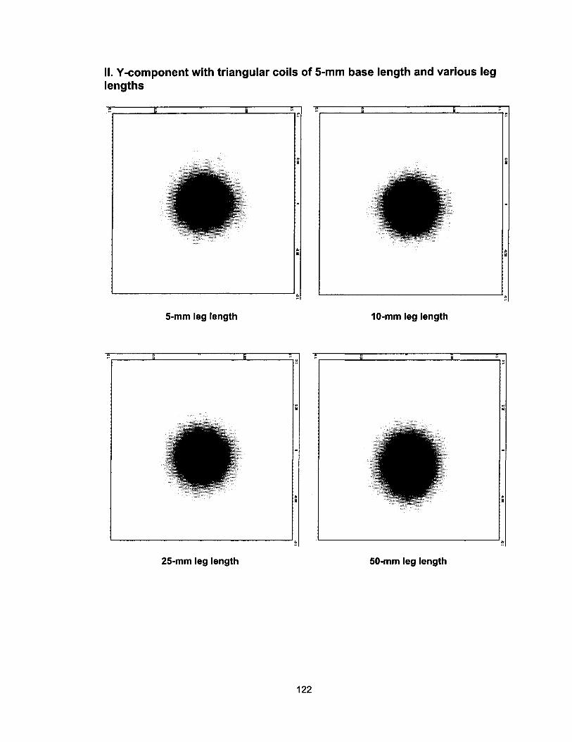
II. Y -component with triangular coils of 5-mm base length and various leg lengths
,"',...-__ ..lL-_____ ----iIl...-__ -=:..,e
S-mm leg length 10-mm leg length
2S-mm leg length SO-mm leg length
122

III. Z-component with equilateral triangular coils of various side lengths
10-mm side length 20-mm side length
30-mm side length 40-mm side length
123

Appendix G: Inverse Analysis Results
The following shows the resulting magnetic flux density distribution after TSVD (left), the resulting dipole locations after data clustering (middle), and the adjusted dipole locations after downhill simplex computation (right) of the sequential inverse analysis steps for test cases 1, 2, 3, 4, 6 and 10.
.. ala
1 al
"'" -ill ~, ....
."
• m
u
.. a
....
lSVD_
u
-ill
u
.lI
1"
"'"
u
... 1.' ....
....
-ii, ....
" '0
• "'" 01
,w
Test case 1
1/1 .. .. \.
.,
Test case 2
--.-~.-- . .. ..
tesfcase3
124
U
.16
1 " . .... -ii, ....
u
... 1°'
-ii, ....
.. .,.
1·' ... -ill ....
"'" ,w
... 'W
_ .......
1/1 ,. .. .. '!' ,
'b en
01
--
"
_ .......
.~.- It
• •
«. "
.. -ill
()

.. . ,. l ., .
l .,
0JI5
-Il' -• 0JI5
Oa:IiI. ~AJ'/ Jt~.~ 1$\/1)_
l .,
0JI5
0 ..
... , -
ut. :s .,
". :SOl .
-Il' -
• 0JI5
0'
Test case 4
'" . • \J _'Ii .,
('
Test case 6
')
,., • 0JI5
" ,(0) ,(oJ
125
.. a"
l" ...
o a: iii. ~
.. 0"
lOl 0JI5
-Il, -
l " ....
-Il' -
., .. (I; •
AJ'/ Jt~0 _ ......
'" .;I'\ "
'" ',r.
... " ,(oJ ,(oJ
_ ......

REFERENCE LIST
[1] N. A. Campbell and J. B. Reece. Biology (8th ed.) 2008.
[2] C. Watson, M. Kirkcaldie and G. Paxinos. The Brain: An Introduction to Functional Neuroanatomy (1st ed.) 2010.
[3] M. Hamalainen, R. Hari, R. J. IImoniemi, J. Knuutila and O. V. Lounasmaa. Magnetoencephalography-theory, instrumentation, and applications to noninvasive studies of the working human brain. Reviews of Modern Physics 65(2), pp. 413. 1993.
[4] H. Preissl. Magnetoencephalography 2005.
[5] R. Rottier. The application of superconductors in medicine. 2000.
[6] W. Haschke, E. Speckmann and A. I. RoAtbak. Slow Potential Changes in the Brain 1993.
[7] S. Baillet, J. C. Mosher and R. M. Leahy. Electromagnetic brain mapping. Signal Processing Magazine, IEEE 18(6), pp. 14-30.2001.
[8] J. C. de Munck, B. W. van Dijk and H. Spekreijse. Mathematical dipoles are adequate to describe realistic generators of human brain activity. Biomedical Engineering, IEEE Transactions on 35(11), pp. 960-966. 1988.
[9] J. Sarvas. Basic mathematical and electromagnetic concepts of the biomagnetic inverse problem. Phys. Med. BioI. 32pp. 11. 1987.
[10] J. Malmivuo and R. Plonsey. Bioelectromagnetism : Principles and Applications of Bioelectric and Biomagnetic Fields 1994.
[11] A. Hillebrand and G. R. Barnes. A quantitative assessment of the sensitivity of whole-head MEG to activity in the adult human cortex. Neuroimage 16(3, Part A), pp. 638-650. 2002.
[12] S. S. Nagarajan. Advances in electromagnetic brain imaging. Presented at Human Vision and Electronic Imaging XV. 2010, Available: http://dx.doLorg/10.1117/12.849117.
126

[13] M. S. Hamalainen and R. IImoniemi. Interpreting magnetic fields of the brain: Minimum norm estimates. Medical and Biological Engineering and Computing 32(1), pp. 35-42. 1994.
[14] R. J. IImoniemi. Estimates of neuronal current distributions. Acta Otolaryngol. 111(S491), pp. 80-87.1991.
[15] S. Baillet, J. Riera, G. Marin, J. Mangin, J. Aubert and L. Garnero. Evaluation of inverse methods and head models for EEG source localization using a human skull phantom. Phys. Med. BioI. 46pp. 77. 2001.
[16] R. M. Leahy, J. C. Mosher, M. E. Spencer, M. X. Huang and J. D. Lewine. A study of dipole localization accuracy for MEG and EEG using a human skull phantom. Electroencephalogr. Clin. Neurophysiol. 107(2), pp. 159-173. 1998.
[17] P. McVeigh, A. Bostan and D. Cheyne. Study of conducting volume boundary influence on source localization using a realistic MEG phantom. Int. Congr. Ser. 1300(0), pp. 153-156.2007.
[18] M. Spencer, R. Leahy and J. Mosher. A skull-based multiple dipole phantom for EEC and MEG studies. Presented at Biomag 96: Proceedings of the Tenth International Conference on Biomagnetism. 2000, .
[19] P. C. Hansen, M. L. Kringelbach and R. Salmelin. MEG: An Introduction to Methods 2010.
[20] J. Clarke and A. I. Braginski. The SQUID Handbook 2003.
[21] NATO Advanced Study Institute on Biomagnetism and S. J. Williamson. Biomagnetism : An Interdisciplinary Approach 1983.
[22] VSM MedTech Ltd., Data Acquisition Guide CTF MEG Software Release 5.4. VSM MedTech Ltd., 2006.
[23] Y. Kishimoto, "Studies of Real-Time Monitoring Techniques by Inverse Analysis of Electromagnetic Field: Applications to LSI Electroplating Control and Brain Function Diagnostics," pp. 117-145,2010.
[24] J. Liu, Y. Kishimoto, T. Cheung, A. M. Parameswaran and K. Amaya. Development of human brainwave simulating device for magnetoencephalography and the corresponding dipole localization study. Presented at 17th International Conference on Biomagnetism Advances in Biomagnetism-Biomag2010. 2010, .
127

[25] G. Uehara, M. Miyamoto, Y. Adachi, Y. Haruta, J. Kawai, T. Shimozu and M. Kawabata. An effect of electrical double layer on MEG phantom with saline water. Presented at International Congress Series. 2007, .
[26] Y. Kishimoto, J. Liu, T. Cheung, A. M. Parameswaran and K. Amaya. Magnetic dipole localization studies for magnetoencephalography using multiple phase inverse analysis and the experimental verification. Canadian Medical and Biological Engineering Conference 2009.
[27] D. Halliday, R. Resnick and J. Walker. Fundamentals of Physics (5th ed.) 1997.
[28] G. Uehara, M. Higuchi, Y. Adachi, J. Kawai, H. Tanaka, Y. Haruta, M. Miyamoto, T. Shimozu and M. Kawabata. An error in magnetic field of isoscelestriangle coil as a representation of equivalent current dipole. Presented at International Congress Series. 2007, .
[29] A. V. Oppenheim, A. S. WHIsky and S. H. Nawab. Signals & Systems (2nd ed.) 1997.
[30] COMSOL AB, COMSOL Multiphysics User's Guide Version 3.3. COMSOL AB,2006.
128