Fertility, Household’s size and Poverty in Nepal · PDF fileFertility, Household’s size and Poverty in Nepal * ... Those who contest this view generally argue that ... between

Fertility, Household’s size and Poverty in Nepal François LIBOIS and Vincent SOMVILLE

CRED - October 2014

Department of Economics

Working Papers

2014/12

Fertility, Household’s size and

Poverty in Nepal*

François Libois2 and Vincent Somville3

October 22, 2014

Abstract

Population control policies keep on attracting massive attention:having more children would directly contribute to household’s poverty.Using household level data from Nepal, we investigate the links be-tween household’s fertility decisions and variations in their size andcomposition. We show that household size barely changes with ad-ditional births but household composition is affected. Couples withfewer children host, on average, more other relatives. This result im-plies that fertility of a household has an ambiguous impact on its percapita consumption which depends on the relative gains in lower con-sumption versus costs of a lower income. We use the gender of thefirst born child to instrument the total number of consecutive childrenand identify the causal relationship.

Keywords: Nepal ; Household size ; Household composition ; Poverty ;Fertility

JEL codes: I32 ; J13 ; D13 ; O53

*We are thankful to Arild Aakvik, Jean-Marie Baland, Catherine Guirkinger, MagnusHatlebakk, Sylvie Lambert and Jean-Philippe Platteau for numerous comments as well asto seminar participants from CRED in Namur, CMI in Bergen, Heriott-Watt University,NTNU Trondheim, Bergen University, The Norwegian School of Economics - NHH andthe NCDE conference in Helsinki. Vincent Somville acknowledges financial support fromthe Research Council of Norway through the Econpop program.

2Centre for Research in the Economics of Development, University of Namur, Belgium.E-mail: [email protected]

3Chr. Michelsen Institute, Norway E-mail: [email protected]

1

1 Introduction.

Policies aiming to lower the fertility of poor people have been carried out inmost developing countries of the world. They have sometimes been dramat-ically violent and invasive, as illustrated by the application of the Chineseone-child policy or the Indian sterilisation campaigns under Sanjay Gandhi.

We focus on fertility’s incidence on households’ composition and poverty.Our starting point is the argument illustrated by Figure 1. This poster ofthe India Ministry of Health and Family Welfare is well representative of thelow-fertility campaigns and similar posters can be found in other countries orat other times. It pictures on the left side a family that has many children:that family is poor, badly dressed, living in a house that is in a very poorcondition and with nothing growing on their land. On the right side there isa family that only had two children and looks much richer and happier. Theyhave a nice house, nice clothes, a fertile land and a tractor. Even the treeregains its leaves when there are only two children. The argument is thatpoor and large families do not have the means to invest (in the education oftheir children, or in the activities that generate their incomes) and, to getout of poverty, the poor should have few children (two children is usuallyadvocated).

Insert figure 1 here

While Becker et al. (1960) established an economic framework to studythe effects of the parents’ income on their fertility, their arguments formallylink the income with the number of children and can be used to analyse thereverse relationship.

The mechanism that is implicitly assumed in the picture can be describedas follows. The household has a limited amount of resources. When oneadditional child is born, the size of the household grows accordingly. Thereis an additional unproductive mouth to feed and therefore income per capitais lower. The household does not have the means any more to invest in theirproductive assets and in the education of their children.

Whether this message is correct or not is however of crucial importanceto the poor. Is it really true that they will become rich and happy if theyrefrain from having children?

It is also crucial to policy makers. According to the picture, fertilitycontrol would be an effective tool to eradicate poverty. Before spending

2

resources on this kind of campaign, or on more aggressive policies as hasbeen done in India and China, policy-makers ought to know exactly whatbenefits to expect in terms of increased incomes and poverty alleviation.

Empirically, the effects of changes in fertility on various outcomes linkedto household’s welfare remain unclear. As Schultz et al. (2007) concludefrom their review of the empirical literature, “Policies that help individu-als reduce unwanted fertility are expected to improve the well being of theirfamilies and society. But there is relatively little empirical evidence of theseconnections from fertility to family well-being and to intergenerational wel-fare gains, traced out by distinct policy interventions. (...) The hypothesisthat policy-induced fertility declines have contributed to increases in familysavings rates is intuitively plausible, as is the life-cycle savings hypothesis.No studies were found, however, to show exogenous sources of fertility de-cline have actually increased family life cycle savings and added over time tothe accumulation of physical assets.” (Schultz et al., 2007,p.3294-3295).

We use data from the Nepal Living Standards Surveys to investigate thelinks between household’s fertility decisions and their consequent achieve-ments in incomes.

First, we check how the size of households evolves with additional births.We find that on average, the size of the households is barely affected by addi-tional births, only the household composition changes. To identify the causaleffect of the number of children on the household’s size and composition, weuse the gender of the first-born as an instrumental variable. Because of astrong preference for sons, Nepalese parents whose first-born is a girl tend tohave more children.

As we show below, the size of the young mothers’ households slightlychanges with an additional birth. The arrival of a new child is compensatedby the absence of another member. On the other hand, older women’s house-holds decrease in size with the number of children. In this latest case, the datashow that couples who had fewer children tend to host more grand-childrenand in-laws than couples with more of their own children. Because house-holds are parts of extended family networks, those who have fewer childrensimply host more other relatives. This finding concurs with the argumentsof Cox et al. (2007) who emphasised the importance of kinship networks inredistributing resources. In our case, people, rather than goods or money,move between households.

When the arrival of an additional child provokes the departure of anotherhousehold member, it is not obvious any more that the household will have

3

fewer resources per person. This will depend on the relative consumptionand generation of income of the child versus the member who left.

Second, we test whether having an additional child leads to a lower level ofincome and consumption. Simply comparing the incomes of small and largefamilies obviously does not allow to conclude anything about the causal effectof the family size on the household’s income: poor parents may have morechildren because they are poor and will need their children support later inlife, or on the contrary, rich parents may decide to have more children becausethey are rich and can afford more children. Despite our best efforts, we do notfind significant correlations between the number of children and the incomeand consumption of households. We explain this absence of correlation byour previous finding, that household size is unrelated to the number of births.

The main result of the paper is that the theoretical prediction that largerfamilies will get poorer does not materialise. Households include variouspeople such as grand-parents, uncles and aunts, cousins, non blood-relatedpeople, etc. When a family has an additional children, some of the otherpeople may move away leaving the size of the household constant. Andsimilarly if a couple has few children at home they are likely to host moreother relatives or acquaintances.1

Clearly, fertility decisions and the way household’s composition and in-comes vary with new births are context-dependent and most likely differentfamilies will adopt different behaviours. Childs (2001) for instance describeshow in Nepal two geographically close villages followed opposite directories interms of population growth. In one village, parents designated their daugh-ters to be nuns, barring them from marriage, while in the other young daugh-ters were getting married and having children. Our goal here is to checkwhether a general pattern emerges across local differences and we focus onaverage effects over a very large sample that covers most of Nepal’s areas.

Other arguments have been used to justify the public control of the sizeof a population. The influence of Malthus (1798) is strong and many call fora limit on the world population given the limited amount of resources thatare available. Those who contest this view generally argue that technologicalprogress creates new resources and more efficient ways to use resources andthat must be taken into account. And a larger population may make creative

1This argument is related to what anthropologists and biologists have called “cooper-ative breeding”, see Kramer (2010). In economics, it is closely related to the argument ofCox et al. (2007) on the role played by kinship networks in the redistribution of resources.

4

ideas and technological progress more likely. Kremer (1993) supports thishypothesis and conclude that for most of human history, societies with largerinitial populations indeed experienced faster technological change. We leaveaside this debate to focus on the household-level dynamics that we outlinedabove.

In the next section, we present the data and the identification strategy.The empirical analysis is conducted in sections 3, 4 and 5. Section 6 con-cludes.

2 Data and empirical strategy.

The Nepal Living Standards Surveys (NLSS) have been carried out in 1995/96,2003/04 and 2010/11 by the Nepalese Central Bureau of Statistics in collab-oration with the World Bank. The surveys follow the World Bank’s LivingStandards Measurement Survey methodology and cover a wide range of top-ics: demography, consumption, income, access to facilities, housing, educa-tion, health, employment, credit, remittances, etc. The quality of the surveyshas been tested by Hatlebakk (2007) who also discusses them in greater de-tails. The details of the sampling, of the methodology and of the execution ofthe surveys are exposed in CBS (2011a). We use data from the three cross-sections. Our estimation sample consists of 8218 households: 2 105, 2 503and 3 610 respectively from the first, second and third survey. The three sur-veys are referred to as T1, T2 and T3 and all monetary values are correctedfor inflation using local prices and reported in 2010 NPR. Information relatedto children ever born comes from a specific section of the questionnaire aboutwomen maternity history. In that section, the respondent is asked about thenumber of children of each woman, the age of those children, their gender,whether they are still living with the household and other demographic in-formations. A drawback of this dataset is that this information is collectedonly if the women are below 50 years of age. To understand the relationbetween number of children, family size and household income per capita,we first assess the causal impact of the number of children on the family sizeand composition. We use, as an instrument, a binary variable that is equalto one if the first born child is a girl and to zero otherwise. The effects ofthe first-born’s gender have been analysed in various papers (Rosenzweig andWolpin, 2000), in Asia (Chowdhury and Bairagi, 1990; Clark, 2000; Drezeand Murthi, 2001; Lee, 2008) and more recently in Sub-Saharan Africa (Mi-

5

lazzo, 2012). As in other countries, there is in Nepal a strong preference forboys. Couples whose first child is a girl are more likely to have another child,hoping it will be a boy (Gudbrandsen, 2013; Hatlebakk, 2012). Given thathouseholds under study do not have the possibility to choose the gender oftheir child, or to know the gender of the baby in utero, they cannot selectthe gender of their offspring.2 Whether their first-born is a girl or a boyis therefore a random event. To be a valid instrument, conditional on thecovariates that we include, the gender of the first-born cannot have a directeffect on our dependent variables: the household’s income and size. But itseffect must go through the number of additional children. Such will not bethe case if for instance (i) the gender of the children affects the reportingof the number of children ever born by their mother, (ii) if the gender ofthe first-born affects the dynamics of household creation (e.g. if a first bornboy becomes the household head), or (iii) if the parents adopt different be-haviours (related to income and the size of their household) because theirfirst-born is a boy rather than a girl). We discuss and test these scenario inSection 7.

One downside of this instrumental variable, is that it can only be used onthe sub-set of people who have had at least one child. This limits its externalvalidity and the results cannot be used to assess the effects of having one childversus not having any children.3 The following terminology is used in theanalysis. A household comprises all people living together at the time ofthe survey. A family is composed of the head of the household, his/herspouse and their children. The size of the household is therefore equal tothe size of the family, minus the number of family members living elsewhere,plus the non-family people living in the household. The income per capitais the total income earned by all household members divided by the size of

2See Valente (2013).3The original dataset contains information about 13 273 households. A total of 4 135

households are dropped from the dataset because their head never had a child yet. Fromthe remaining data, we drop 748 households for which the maternity section is missingbecause the mother is above 49 years old and we further discard 149 households withtwins. The results are not affected by the inclusion of households with twins, but theycomplicate the discussion and the interpretation of some results without generating anyimportant insight. Finally, we lose 23 households with missing data about the age of thehead. Also note that one observation is dropped when we include both the sex of thefirst born and ward fixed effects in the regressions because of perfect multi-collinearity.In income regressions, we further lose 40 households with incomplete information aboutincome.

6

the household. We also refer to the head of the household, his/her spouseand their children when we use the terms nuclear members. Child andchildren are used to identify the sons and daughters of the household head.While a child is obviously younger than his father, children can be old. Theycomprise babies and infants but also adult children. We count all the childrenever born, including those that were dead at the time of the survey.4

3 Empirical analysis.

As shown in Table 1, there has been an important increase in income percapita in Nepal between the surveys. The mean income per capita more thantripled and the median doubled. This change is both driven by the increaseof the absolute level of income and by the significant reduction in householdsize. First, absolute income increase is related to the expansion of non-farmactivities and to growing in-flow of remittances (see CBS, 2011b). Noticethat the mean in the last survey is heavily influenced by a few extremelyhigh incomes. The income of the 25th, 50th and 75th percentiles nonethelessall doubled over the period, indicating similar decreases in poverty over thedifferent initial levels of income. Second, household size goes down and itcorrelates to a decline in fertility. On average, household heads have had4 children in the first survey, 3.65 in the second survey and 3.3 in the lastsurvey. The median number of children went down from four to three. On theother hand, the median household size did not change as much: the mediannumber of household members remained constant and equal to 5 over allthree surveys.

Insert table 1 here

Figure 2 breaks the mean household per capita income down for differentoffspring numbers. From this picture, it is clear that households that havebetween one and three children have on average higher incomes per capitathan households with more children. There is however no clear difference inincomes between the households that have one, two or three children. Thereis neither a difference in incomes among the households that have more thanthree children. The negative correlation between the number of children and

4Our results are robust to the use of the number children still alive at the time of thesurvey.

7

household income per capita is consistent with the expectations that poorerparents decide to have more children to have a guaranteed support later inlife. It could be as well that having more children increases the pressure onthe household’s resources, and decreases per capita income.


3.1 Preference for boys.

As already mentioned, we use the gender of the first child as an exogenousdeterminant of the total number of children. This instrument has both statis-tical relevance and anthropological soundness. Table 8 shows that on average,at the time of the survey the couples had 3.8 children if they first had a girland 3.4 children if they first had a boy. The median number of children is4 among the families with a first born girl and 3 among the families with afirst born boy. Figure 3 shows that there is first order stochastic dominanceof the number of births distribution in first born girl families over first bornboy families.5 This is in line with our expectations that people keep havingchildren as long as they don’t reach their desired number of boys.

Insert table 8 here


Onesto (2005) summarizes the preference for boys by quoting a countrysidesaying: “To get a girl is like watering a neighbor’s tree. You have the troubleand expense of nurturing the plant but the fruits are taken by somebody else.”A daughter “is useful and valuable in her childhood years when she can dochores and serve the household”. Afterwards, she marries and all long terminvestment benefits flow to her husband. In a more in-depth study of aTamang community, Fricke (1986) reports that there is a slightly greaterdesire for male children but that babies are equally treated. Women providelabour force as long as there are member of the household and form a cornerstone of extended reciprocity relationships. However, sons remain the onlyone who formally inherit land and who take (financial) charge of their parents

5This is confirmed by a two-sample Wilcoxon rank-sum test which rejects the equalityof distributions with an associated p-value < 0.0001

8

funerals. Inability of a women to have sons is almost one of the only reasonsto observe polygyny.

Nepalese have at least two good reasons to wish to have at least two boys.As already mentioned, boys traditionally inherit the family’s land. Having aboy to take care of the land and inherit the family’s assets is the tradition.In addition, it is easier for a boy to migrate. In the last couple of years,the returns to migration are very high and remittances constitute a veryimportant part of household’s revenues (CBS, 2011b). Families also reportwanting a second boy to get an education while the first takes care of theland. Additionally, it is a son who is supposed to lit the parents’ funeralpyre.

Under the assumptions that the sex ratio at birth is equal to 0.5 andthat the number of children is not bounded, if households want to havetwo boys and don’t especially want girls, then the probability to observe n

children in a household is equal to (n − 1) (0.5)n. The process behind thisprobability is depicted in the appendix (see figure A.1). In Table 3, wecompare the expected number of children under the rule “having two boys”,to the real number of children in the data (we use the sample of householdswith at least 2 children). The similarity between the expected and observednumbers is striking ; we interpret it as a complementary evidence in favourof our instrument.6

Insert table 3 here

3.2 The different household members.

As we can see from Table 4, households are composed of people with variouslinks to the household head. 43.62% of individuals in our sample live in non-nuclear families. The number of households that match the picture in Figure1 is in fact quite small. Only 14.4% of the households have two children andlive in a household that is only composed of the parents and their children.7

6Obviously, if households aim at having two girls instead of two boys, we obtain thesame predicted number of children. This table nonetheless shows that the data are consis-tent with the assumption that households aim at having two children of a certain genderwhile we could not find any anthropological argument to support the “two girls hypothe-sis”.

7This proportion drops to 10.2% in the whole sample survey, including householdswithout any birth.

9

Insert table 4 here

In the appendix, we show how the composition of households correlateswith some of their characteristics. Table A.1 displays the evolution of house-hold average composition through the life-cycle of its head. The size of thehousehold is relatively constant, it varies from 4.49 (youngest heads) to 5.78(50-60 years old). The number of births increase: the 20% youngest headshave on average 2.3 children and the oldest have 4.6.8 Globally, householdscomposition changes as follows: when the head gets older, he/she lives with(i) less of his children, parents, siblings and siblings-in-law and (ii) moreof his grand-children and children-in-law. All-in-all, the average number ofpeople in the household barely changes and remains close to the average of5.22 people in all five categories. Note that despite an increase in the num-ber of births as heads get older, the number of children in the householdactually follows an inverted-u shape relationship. In Table A.2, we displayhow the household composition evolves with the number of births from thehead. The average number of children living in the household increases byless than one with an additional birth. Couples that have few children are (i)more likely to live with their parents, siblings, nephew and nieces, or otherrelatives, they are (ii) less likely to live with their spouse, grand-childrenand children-in-law. In Table 5, the composition of the households is dividedbetween households with a first born girl or boy. The table confirms thathouseholds with a first born girl tend to have more children, 3.79 on averageagainst 3.4 if the first born is a boy. However those with a first born boytend to host more children-in-law and grand-children. This is consistent withthe Nepalese patriarchal habits. The daughters tend to leave the householdwhile sons stay longer, potentially with their wife and first children.


3.3 Additional summary statistics.

The covariates used in the regressions are summarised in Table 6. A house-hold head is on average 39 years old, and four times out of five, a male. Theaverage age of mothers is 35, but this is an underestimation since mothers

8The next columns show the average number of the member type in the age category.For instance, the households of the heads that are less than 30 years old include on average0.7 spouse, 2.13 children, 0 grand-child, 0.23 parents, etc.

10

older than 49 do not respond to the maternity file. Polygyny is rare withonly 1% of households having a head with two spouses. Nepali householdsare on average quite poor with a thin asset ownership as well as low incomeand consumption expenditures9. We also provide the share of the householdsliving in the Terai or in the Hills. Less than 8% of our sample comes from theMountains. Note that all regressions include ward fixed effects and thereforecontrol for all variables that are constant at the ward level.

4 Number of children and household size

We first look at the effect of the total number of children on household sizeand show that, on average, the net effect is barely positive. As we explainedabove, we use the gender of the first born child as an instrument for the totalnumber of children. Presumably, the effect will depend on the mother’s age.We observe that households with more children host less non-nuclear relativesand do not host more nuclear relatives in the long run. The replacementeffect is nonetheless not instantaneous. An additional birth first increasesthe household size and decreases it only after some time. To capture thiseffect, we include the mother’s age and the interaction between the mother’sage and the number of births in our regressions.10 We estimate equation(1), where the dependent variable yitw has a value for each household i attime t in ward w and is given by: whether the household is composed ofnuclear relatives only (Table 7) ; the number of household members (Table8) ; the number of nuclear members (Table 9) ; the number of extended familymembers (Table 10). Our main variables of interest are: Kitw, the numberof children of the household’s head ; Aitw, the mother’s age and Kitw ∗ Aitw,the interaction between both variables. X is a vector of control variablespresented in Table 6 with associated parameter vector Φ. Regressions alsoinclude time and ward fixed effects. We cluster the standard errors at the

9Consumption expenditures do include food monetary expenses, a valuation of homeconsumption, infrequent expenditures, health related expenses and housing expenses (rent,water, electricity, garbage, communication, fuel). It does not include the purchase ofproductive inputs nor of durable assets. Income is the sum of all wage incomes frompermanent and casual employment, income from self-employed activities, in agricultureor outside, including a market price valuation of home consumption, capital income andtransfers received.

10Results are qualitatively similar if we run separate estimations by mother’s age inter-vals.

11

ward level.11

yitw = β1Kitw + β2Aitw + β3Kitw ∗ Aitw + XitwΦ + αw + δt + εitw (1)

4.1 The gender of the first born instruments the num-

ber of children.

In Tables 7 to 10, we estimate the effect of one additional child on householdstructure. We use four dependent variables: (i) the probability to observea nuclear household, (ii) the size of the household, equal to the numberof household members, (iii) the number of nuclear members, where we onlycount the head, his spouse(s) and their children, and (iv) the number of othermembers, that is the household size minus the number of nuclear members.In the four tables we first present ordinary least squares regressions, and thentwo stage least square regressions. We control for some household character-istics that may also affect the household structure as well as for productiveassets owned by the households. Household characteristics are head’s gen-der, a dummy identifying polygynous households, ethnicity dummies as wellas head’s age and its square and mother’s age. The last two covariates aimat capturing generational effects. Productive assets include the amount ofland and the number of cows owned, the average education level among theadults of the household, and a binary variable equal to one if the householdowns a non-agricultural business. All regressions also include time and ward(village) fixed effects. The standard errors are clustered at the ward level.On top of a direct effect of age on the household structure - which is cap-tured by the controls mentioned above, the number of children might have aheterogeneous effect on household structure across time. Therefore, we addan interaction term between the mother’s age and the number of children.That interaction is instrumented by the interaction between the mother’s ageand the gender of her first born child. Notice that our results are unaffectedby the inclusion of the age of the first born among the controls. In Table 7,according to the 2SLS estimates, having one more child decreases the prob-ability of hosting extended family members by 6%. In column (7), we seethat the negative effect of an additional child becomes stronger with time.

11All our regressions with instruments are estimated using xtivreg2, developed in Schaffer(2012).

12

The older the mother is at the time of the survey, the lower is the probabilitythat she hosts non-nuclear family if she had more children, as shown on thefirst column of figure 4, which presents the estimated marginal effect of anadditional child on the probability to observe a nuclear household in functionof mother’s age.


Table 8 shows that on average, having one more child leads to house-holds having 0.34 more members (column 3). The positive effect is weaker(stronger) for older (younger) mothers. This average positive effect is drivenby the number of nuclear members who increases by around 0.59 for each ad-ditional birth (Table 9, column 3). Conform to the intuition, the number ofnuclear members do increase more when the mother is young as depicted inTable 9. On the other side, an additional birth decreases the average numberof non-nuclear members by 0.25 member (see Table 10). This effect is clearlydriven by households with older mothers. For instance, households host 0.57less other members when mothers are 40 years old. The second column offigure 4 and figure 5 respectively summarize these effects for household sizeand household composition.


Our result contributes to the understanding of household splits. By de-composing effects across relations to the head, we see that the positive effecton household size effectively comes from an increase in the number of head’schildren living with their parents. This is counter-balanced by a decrease indaughters-in-law and grand children hosted by the household, as shown intable A.6 and A.7 as well as figure 6. Larger offspring implies earlier house-hold splits. In his study of a Tamang village, Fricke (1986) notice that splitdecisions (and consequently the moment at which men take their inheritance)are highly strategic. “A Tamang male (...) is constantly weighing the hap-piness of his wife in a home where she has no power, the size of his familyand the potential for his inheritance to grow from the continued acquisitionsof his father and brothers.”(p143)

As we emphasised in the introduction, the literature assumes a mechanicallink between the number of children and the households’ income per capita.By increasing the number of capita, but without contributing substantially to

13

the income, additional children are expected to impoverish the households. Inthis section, we have however shown the lack of effect of additional childrenon household size. The expected mechanism does not materialise becausethe arrival of a new nuclear-members in the household is compensated by asimilar reduction in the number of other members.

Consequently, new births also affect the adult/children ratio in the house-holds. As shown in Table 11, an additional birth increases the number ofchildren in the household. On the other hand, it decreases the number ofadults in the household as we can see in Table 12 and in figure A.2. Thischange in the household composition is crucial to assessing the links betweenfertility and poverty. It is usually accepted that a child consumes less thanan adult. And therefore, an additional birth could either increase or decreasethe household’s consumption per head, depending on the importance of thegains in consumption versus the potential loss in income. We turn to thatquestion in the next two sections.

5 Number of children and household’s income

and consumption.

Policies aiming at reducing fertility implicitly assume that additional birthsdecrease household per capita income. Indeed, if additional children do notcontribute substantively to the household’s income, but increase the numberof people in the household, they must decrease the per capita income. Weestimate the correlation between the number of children and the householdincome and consumption. To take into account changes in the compositionof the household (more children and less adults), we also use the OECD -modified scale to adjust the household size. That scale assigns a value of 1to the household head, of 0.5 to each additional adult member and of 0.3 toeach child.

Our regressions are similar to those presented in the previous section andwe use the same instrument. We test the correlation between the householdincome and the number of children in Tables 13 and 15. We test the cor-relation between the household consumption and the number of children inTables 14 and 16. The four tables have the same structure. The first threecolumns show OLS regressions of (i) the dependent variable (the logarithm ofthe household income or consumption) (ii) the dependent variable divided by

14

the household size and (iii) the dependent variables divided by the adjustedhousehold size. The next columns show the first and second stages of 2SLSestimations of the same variables. Tables 15 and 16 differ from Tables 13and 14 ; they include an interaction term between the mother’s age and thenumber of children.

As we can see in column (1) of Table 13, there is a positive correla-tion between the number of children and households income. This positivecorrelation vanishes when the number of children is instrumented. In IV es-timations, there is no indication of a positive correlation, and if somethingcomes out, it is negative. The number of children however has a significantnegative effect on the household per capita income (and adjusted per capitaincome), reflecting the effect of the additional births on the household’s size.

Based on results of the previous section, conclusions have to adapted withrespect to mother’s age since household composition is highly dependanton mother’s age and number of births. Having more children increases thenumber of nuclear members when the mother is young. As time passes,mothers who had more children host less other relatives and their householdsize declines.

As expected from our results about the evolution of the household size, thecoefficient of “# children” is negative but the interaction with the mother’sage has a positive coefficient. We again note the absence of significant corre-lation between the number of children and the household’s income (column6). There is neither any significant correlation between the number of chil-dren and the household’s income per capita when it is adjusted with theequivalence scale (column 8). Looking only at the household’s income percapita, both variables have statistically significant coefficients. The youngestmother in our sample is 17 years old. The interacted coefficient (Mother’sage*# children) therefore becomes 17 ∗ 0.02 = 0.34 for the youngest mother.The Wald test fails to reject the hypothesis that the coefficient of “# chil-dren” is equal to −0.34. Hence, we cannot reject the hypothesis that theeffect of the number of children on the household income per capita is null.

In Tables 14 and 16 we repeat the same analysis but with the householdconsumption instead of the household income. Results are similar. We finda significant and negative effect (Table 14) that dissipates when we takeinto account the mother’s age (Table 16). Again, at the 0.05 rejection level,we cannot reject the hypothesis that the coefficients of “# children” and“Mother’s age*# children” cancel out (the most demanding Wald test iswhen the Mother’s age equals seventeen, the youngest mother, leading to

15

valid conclusions for the the older mothers as well).

6 Estimating a poverty-neutral equivalence

scale.

Instead of using a standard equivalence scale as we did in the previous section,we now estimate the equivalence scale that is such that an additional birthon average leaves the income per capita constant. Consider a householdwith income I. It had B births, and is composed of N people: C childrenand A adults. The adjusted number of people in the household is equal toM = A + xC where x is the scale parameter that we are looking for. Theeffect of an additional child on the household’s adjusted income per capita isgiven by:

(

I

M

)

′

=I ′M − IM ′

M2(2)

We look for x such that(

I

M

)′

> 0, that is:

I ′ (A + xC) − I (A + xC)′

(A + xC)2> 0 (3)

Which can be written as:

{

x > IA′−I′A

CI′−C′I

if CI ′ > C ′I

x < IA′−I′A

CI′−C′I

otherwise(4)

The mean number of adults, children and the mean incomes in the sampleare: I = 193, A = 2.71 and C = 2.51. Without interaction with the mother’sage, the estimated coefficients are: A′ = −0.205, C ′ = 0.534 and (lnI)

′

=−0.04 ⇔ I ′ = I(lnI

′

= −0.04 ∗ 193 = −7.72. On average, an additionalbirth leads to an increase in the adjusted household’s income per capita ifx < 0.34. Note that this is very close to the standard equivalence scales. Inother words, if a child consumes less than a third of what an adult consumes,then the negative effect of an additional birth on the household’s income ismore than compensated by the reduction in the number of adult members,and the income per capita increases.

16

7 Results in perspectives.

In this section we discuss alternative channels which might explain our resultsand we show that our story is robust.

First, sex ratio at birth are stable across birth ranks and remain close to108 boys for 100 girls. This is consistent with medical wisdom and meansthat systematic under-reporting of girls, and therefore of total number ofbirths, is not an issue in our data. Under girl under-reporting, householdswith fewer children would have relatively less girls, less nuclear membersand relatively more non-nuclear members. This, by itself, could explain ourresults but is clearly ruled out by basic descriptive statistics on the sex of thefirst born across birth ranks. On top of that, our results hold when we usethe number of children alive instead of the number of births. It rules channelgoing through gender biased infant mortality rate. It advocates in favour ofother mechanisms explaining the difference between OLS and IV estimates.

Second, a more salient source of bias comes from the absence of futureyoung mothers who have not yet given birth. Their absence in our sampledrives the effect of additional births on the departure of non-nuclear membersdown except if we think that some non-nuclear members would join thehousehold at the first birth. A more realistic mechanism is the devolution ofheadship at the arrival of the first born boy. Under this mechanism, the birthof a boy would transform the head and spouse in parents, the father into ahead, former head’s children into siblings of the new head, the mother intohead’s spouse, ... The birth of a girl would only add a grand-daughter in thehousehold while leaving the rest of household structure unchanged. We donot however find any significant relationship between the sex ratio of the firstborn and the age of the head nor with the age of the head’s spouse. At theopposite of the age spectrum, the absence of old mothers goes in favour ofour conclusions if the trend that we observe before 50 years of age stabilizesor even continues. It means that the average household size would be evenless affected by the number of children.

Third, to check that our results are not driven by the order of the gender-birth sequence, we provide additional tables where we repeat the same anal-ysis but using the gender of the second child as an instrument for the numberof consecutive births. In Tables A.3 to A.5, we only consider heads who haveat least 2 children. We control for the gender of the first child. We instru-ment the number of additional children by the gender of the second child.This process allows us to check that the results are not driven directly by

17

the gender of the first child by relaxing the exclusion restriction on the firstborn. It could indeed be argued that the first boy, who is the heir, is specificand that his gender could play a direct role on how the parents compose theirhousehold. This strategy also allow us to control for the gender compositionamong older siblings, and eventually for the birth spacing between the firstand the second born. The results are robust over these Tables and consistentwith our findings so far: an additional child increases the number of nuclearmembers but decreases the number of other members by a similar amountand the household size barely changes12.

In conclusion, our instrumental variable approach shows that additionalchildren increase the number of nuclear members but decrease the number ofnon-nuclear members. This is especially true when head’s children becomeolder, leading to their departure and to the absence of the head’s daughters-in-law and grandchildren in large sibship. The direction of the OLS bias withrespect to IV estimates indicates that household size has a positive feedbackeffect on the number of children. This can be explained by a preference forlarge households in households with more members or by scale economies inlarger household decreasing the cost of child bearing.

8 Conclusion

Analysing data from around eight thousand households surveyed in the NepalLiving Standard Surveys, we find little correlation between the number ofchildren of a couple and their household’s total income and per capita income.To avoid endogeneity biases, we use the gender of the first born child as aninstrument for the total number of children.

If the household’s total income and per-capita income are barely inde-pendent from the number of children, it must be that the number of childrenbarely affects the number of people in the household. That is precisely whatwe have shown and explained. The more children a couple has and thefewer other people they will host, leaving the household size almost con-stant. Nepalese households are embedded into larger social networks andthose households with fewer children tend to host more other people.

The regressions paint a very clear picture, an additional child increasesthe number of nuclear family members but decrease the number of other hosts

12Note that using the sex of the first two born as instrument for the number of childrenyields qualitatively similar conclusions

18

by a similar amount, leaving the household’s size unchanged over householdlife cycle.

This result has important policy implications. In particular, it predictsthat population control policies should not be expected to have a large impacton poverty levels.

The argument relies on uncoordinated and independent fertility decisionsbetween households. It should be clear that if all households have fewerchildren, and the population size decreases, the average size of the householdsmust decrease (or the number of households must decrease). In this case, theusual presumption that fewer children will translate into higher incomes percapita may be true. More precisely, if the average size of households does notgrow with the number of children that people have, an increase in populationsize should be expected to increase the number of households rather than thesize of each household. This could have important consequences in terms ofpoverty and environmental impact.

Numerous goods are public at the household level, from the primary con-sumption goods such as a common roof or heating, to more complex prod-ucts such as insurance arrangements. It follows that increasing the numberof households rather than the average size of households should result in alower consumption per capita that could not be captured in our study. Sim-ilarly, public bads and pollution are prominent at the household rather thanindividual level. As Axinn and Ghimire (2011) argue, households rather thanpeople determine for instance land use and deforestation. These importantquestions could not be answered here.

We also estimate the consumption equivalence scale that leaves the house-hold’s consumption per capita unaffected by an additional birth. Accordingto our estimates, if a child consumes less than what an adult consumes, thenthe negative effect of an additional birth on the household’s income is morethan compensated by the reduction in the number of adult members, andthe income per capita increases.

Finally, the changes in income in Nepal over the last decade are impres-sive. They are not due to changes in fertility and the underlying forces thatgreatly reduced poverty therefore remain to be explained.

19

References

Axinn, W. G. and Ghimire, D. J. (2011). Social organization, population,and land use. American Journal of Sociology, 117(1):209–258.

Becker, G. S., Duesenberry, J. S., and Okun, B. (1960). An economic analysisof fertility. In Demographic and Economic Change in Developed Countries,pages 225–256. Columbia University Press.

CBS (2011a). Nepal living standards survey household 2010-2011. StatisticalReport Vol. 1, Nepal Central Bureau of Statistics.

CBS (2011b). Nepal living standards survey household 2010-2011. StatisticalReport Vol. 2, Nepal Central Bureau of Statistics.

Childs, G. (2001). Demographic dimensions of an intervillage land disputein nubri, nepal. American Anthropologist, 103(4):1096–1113.

Chowdhury, M. K. and Bairagi, R. (1990). Son preference and fertility inbangladesh. Population and Development Review, 16(4):749–757.

Clark, S. (2000). Son preference and sex composition of children: Evidencefrom india. Demography, 37(1):95–108.

Cox, D., Fafchamps, M., Schultz, T. P., and Strauss, J. A. (2007). Chapter 58extended family and kinship networks: Economic insights and evolutionarydirections. In Handbook of Development Economics, volume Volume 4,pages 3711–3784. Elsevier.

Dreze, J. and Murthi, M. (2001). Fertility, education, and development:Evidence from india. Population and Development Review, 27(1):33–63.

Fricke, T. E. (1986). Himalayan households: Tamang demography and do-mestic processes. UMI Research Press.

Gudbrandsen, N. H. (2013). Female autonomy and fertility in nepal. SouthAsia Economic Journal, 14(1):157–173.

Hatlebakk, M. (2007). LSMS data quality in maoist influenced areas of Nepal.CMI Working Paper WP 2007: 6.

20

Hatlebakk, M. (2012). Son-preference, number of children, education andoccupational choice in rural nepal. CMI Working Paper, 8.

Kramer, K. L. (2010). Cooperative breeding and its significance to the demo-graphic success of humans. Annual Review of Anthropology, 39(1):417–436.

Kremer, M. (1993). Population growth and technological change: One millionB.C. to 1990. The Quarterly Journal of Economics, 108(3):681–716.

Lee, J. (2008). Sibling size and investment in children’s education: An asianinstrument. Journal of Population Economics, 21(4):855–875.

Malthus, T. R. (1798). An Essay on the Principle of Population, as it affectsthe future Improvement of Society, with Remarks on the Speculations ofMr. Godwin, M. Condorcet, and Other Writers. J. Johnson, London, 1stedition.

Milazzo, A. (2012). Son preference, fertility, and family structure. evidencefrom reproductive behavior among nigerian women. Bocconi University.

Onesto, L. (2005). Dispatches from the People’s War in Nepal. Pluto P.

Rosenzweig, M. R. and Wolpin, K. I. (2000). Natural "Natural experiments"in economics. Journal of Economic Literature, 38(4):827–874.

Schaffer, M. E. (2012). Xtivreg2: Stata module to perform extended iv/2sls,gmm and ac/hac, liml and k-class regression for panel data models.Boston College Department of Economics, Statistical Software Compo-nents, S456501.

Schultz, T. P., Schultz, T. P., and Strauss, J. A. (2007). Chapter 52 pop-ulation policies, fertility, women’s human capital, and child quality. InHandbook of Development Economics, volume 4, pages 3249–3303. Else-vier.

Valente, C. (2013). Access to abortion, investments in neonatal health, andsex-selection: Evidence from nepal. Journal of Development Economics,Forthcoming.

21

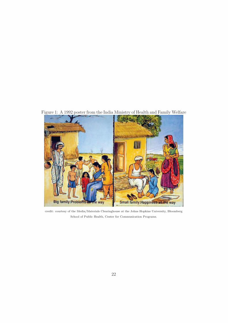
Figure 1: A 1992 poster from the India Ministry of Health and Family Welfare

credit: courtesy of the Media/Materials Clearinghouse at the Johns Hopkins University, Bloomberg

School of Public Health, Center for Communication Programs.

22

Figure 2: Number of children and incomes in the household

23

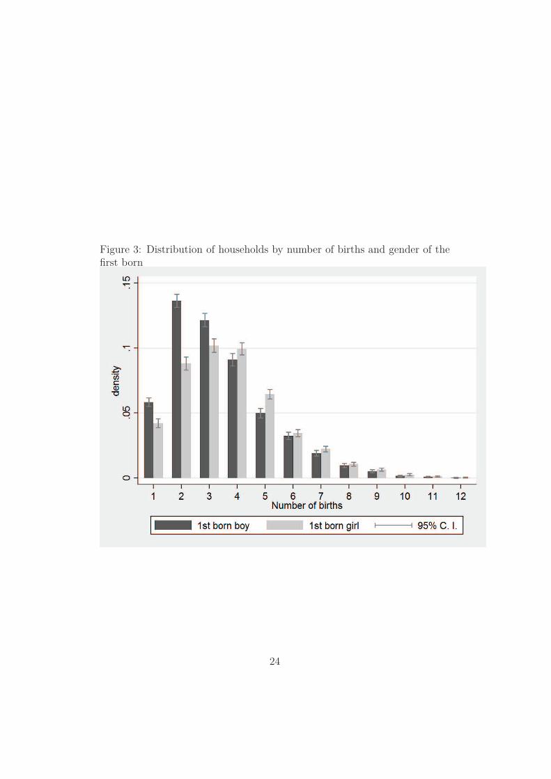
Figure 3: Distribution of households by number of births and gender of thefirst born

24

Figure 4: Marginal effect of an additional birth on household size and form

25

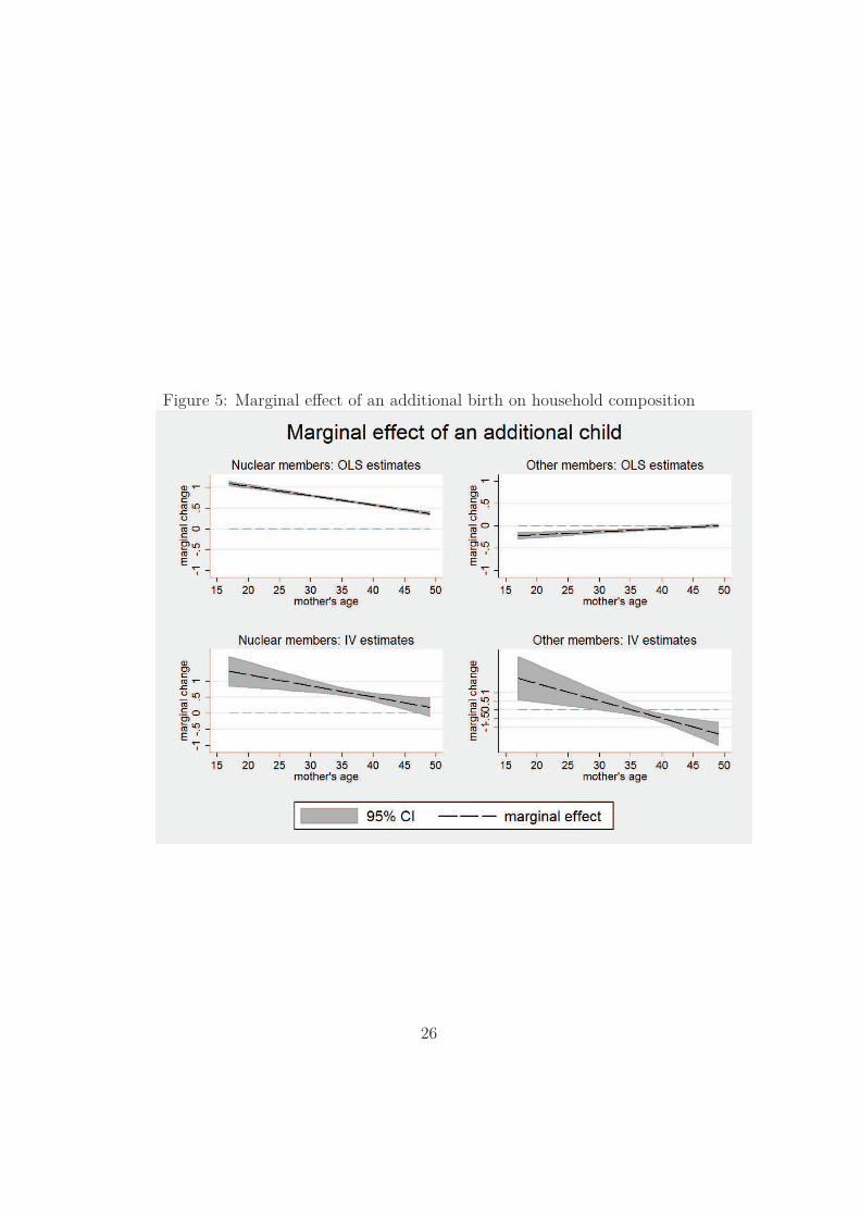
Figure 5: Marginal effect of an additional birth on household composition

26

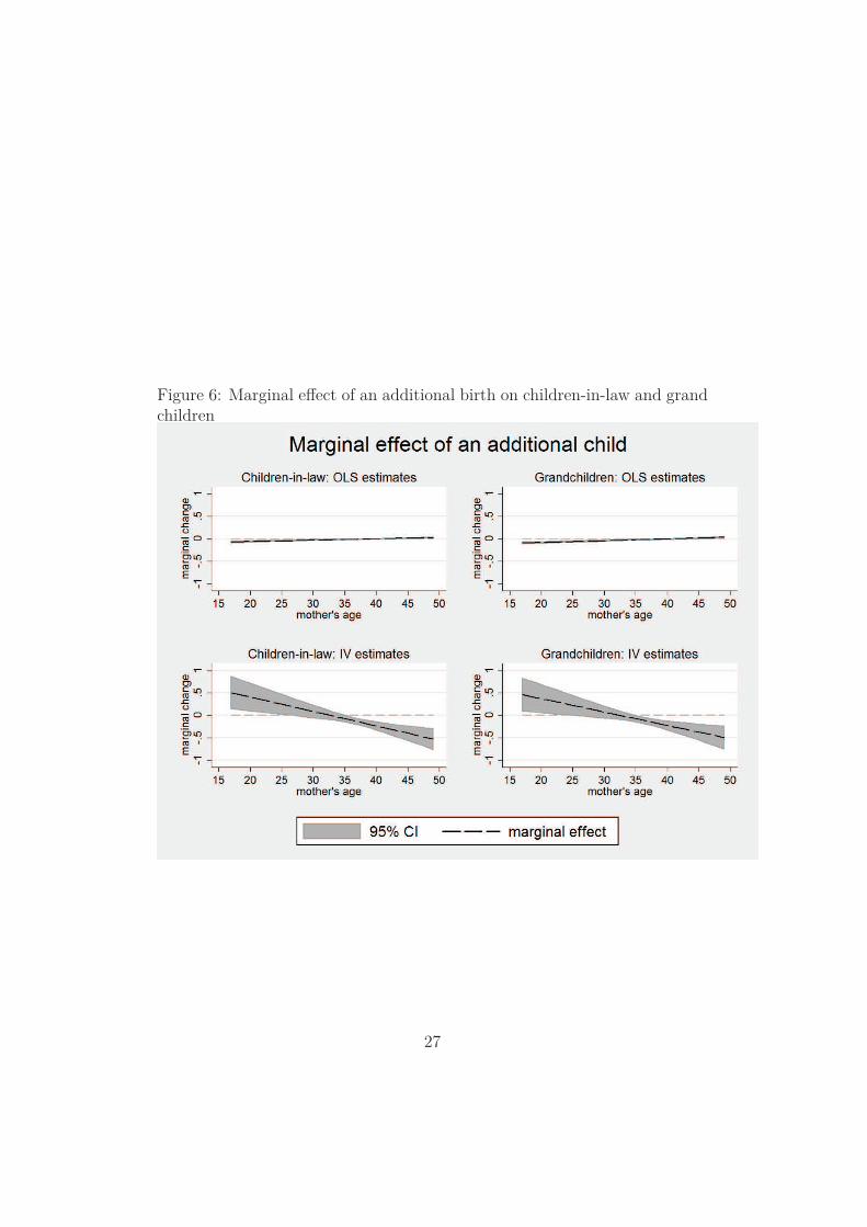
Figure 6: Marginal effect of an additional birth on children-in-law and grandchildren

27

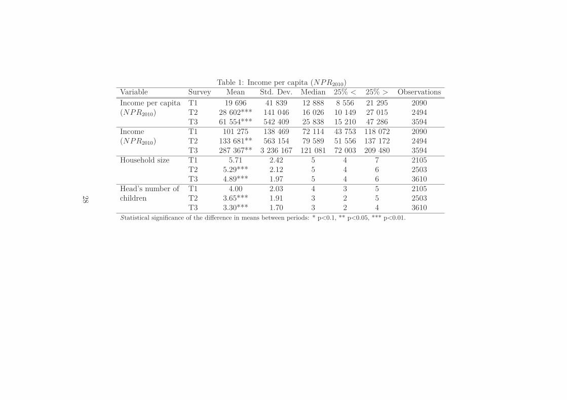
Table 1: Income per capita (NPR2010)Variable Survey Mean Std. Dev. Median 25% < 25% > Observations

Income per capita T1 19 696 41 839 12 888 8 556 21 295 2090(NPR2010) T2 28 602*** 141 046 16 026 10 149 27 015 2494

T3 61 554*** 542 409 25 838 15 210 47 286 3594Income T1 101 275 138 469 72 114 43 753 118 072 2090(NPR2010) T2 133 681** 563 154 79 589 51 556 137 172 2494

T3 287 367** 3 236 167 121 081 72 003 209 480 3594Household size T1 5.71 2.42 5 4 7 2105

T2 5.29*** 2.12 5 4 6 2503T3 4.89*** 1.97 5 4 6 3610

Head’s number of T1 4.00 2.03 4 3 5 2105children T2 3.65*** 1.91 3 2 5 2503

T3 3.30*** 1.70 3 2 4 3610Statistical significance of the difference in means between periods: * p<0.1, ** p<0.05, *** p<0.01.

28

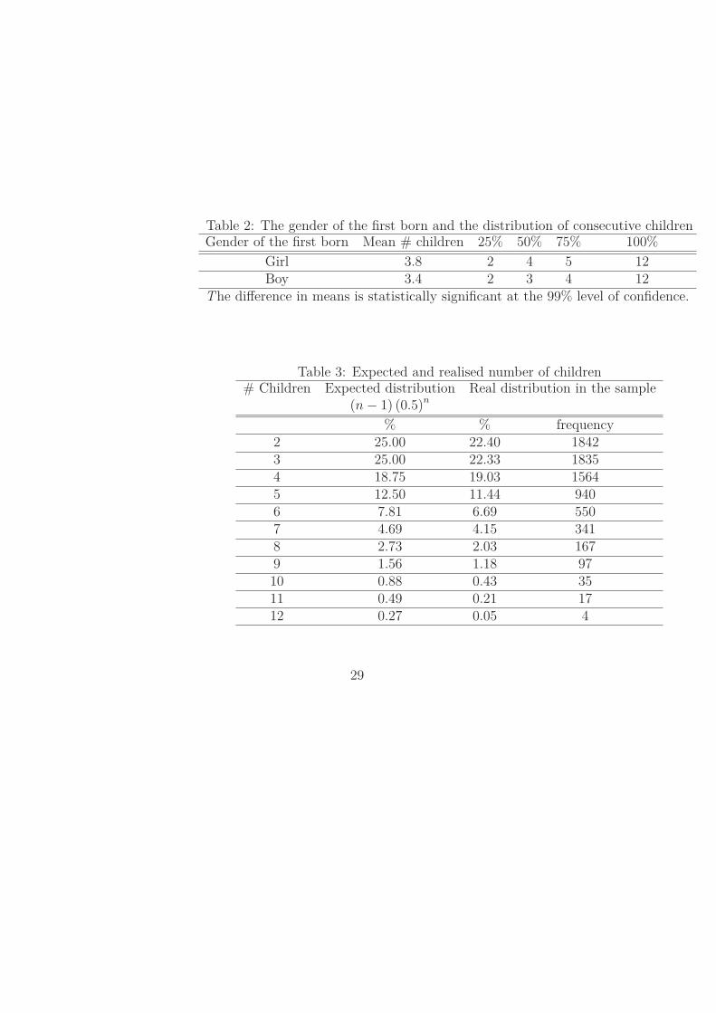
Table 2: The gender of the first born and the distribution of consecutive childrenGender of the first born Mean # children 25% 50% 75% 100%

Girl 3.8 2 4 5 12Boy 3.4 2 3 4 12

The difference in means is statistically significant at the 99% level of confidence.

Table 3: Expected and realised number of children# Children Expected distribution Real distribution in the sample

(n − 1) (0.5)n

% % frequency2 25.00 22.40 18423 25.00 22.33 18354 18.75 19.03 15645 12.50 11.44 9406 7.81 6.69 5507 4.69 4.15 3418 2.73 2.03 1679 1.56 1.18 9710 0.88 0.43 3511 0.49 0.21 1712 0.27 0.05 4

29

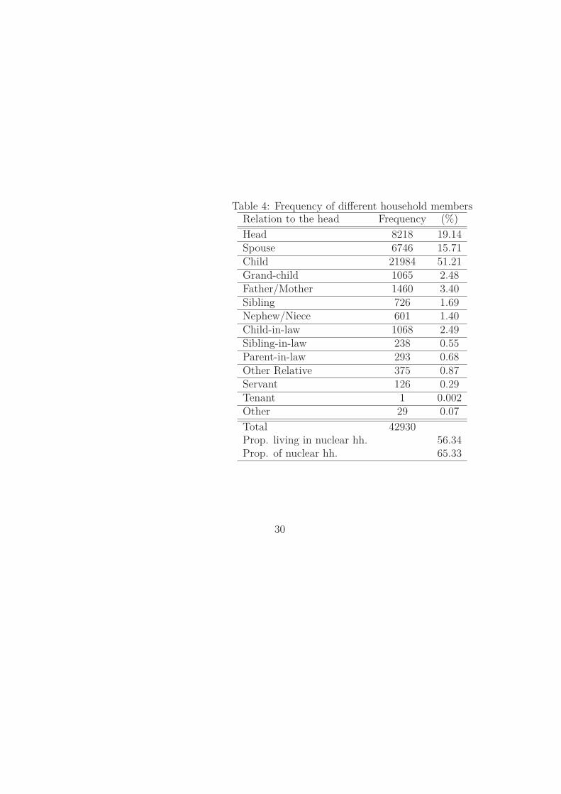
Table 4: Frequency of different household membersRelation to the head Frequency (%)

Head 8218 19.14Spouse 6746 15.71Child 21984 51.21Grand-child 1065 2.48Father/Mother 1460 3.40Sibling 726 1.69Nephew/Niece 601 1.40Child-in-law 1068 2.49Sibling-in-law 238 0.55Parent-in-law 293 0.68Other Relative 375 0.87Servant 126 0.29Tenant 1 0.002Other 29 0.07

Total 42930Prop. living in nuclear hh. 56.34Prop. of nuclear hh. 65.33

30

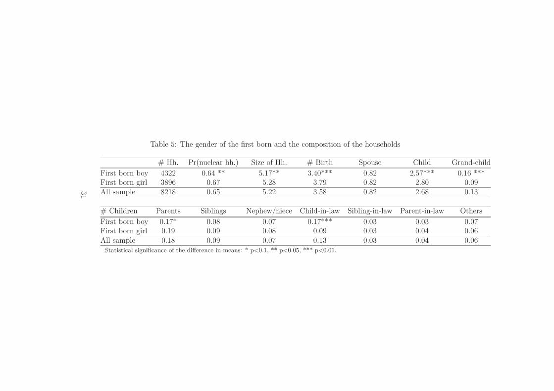
Table 5: The gender of the first born and the composition of the households

# Hh. Pr(nuclear hh.) Size of Hh. # Birth Spouse Child Grand-child

First born boy 4322 0.64 ** 5.17** 3.40*** 0.82 2.57*** 0.16 ***First born girl 3896 0.67 5.28 3.79 0.82 2.80 0.09All sample 8218 0.65 5.22 3.58 0.82 2.68 0.13

# Children Parents Siblings Nephew/niece Child-in-law Sibling-in-law Parent-in-law Others

First born boy 0.17* 0.08 0.07 0.17*** 0.03 0.03 0.07First born girl 0.19 0.09 0.08 0.09 0.03 0.04 0.06All sample 0.18 0.09 0.07 0.13 0.03 0.04 0.06

Statistical significance of the difference in means: * p<0.1, ** p<0.05, *** p<0.01.

31

Table 6: Summary statistics of the main covariates

Variable Mean Std. Dev. Min. Max. N

Male head 0.78 0.42 0 1 8218Age of head 39.05 9.1 18 80 8218Mother’s age 35 7.67 17 49 8218# spouses 0.79 0.43 0 2 8218Household’s size 5.22 2.16 1 29 82181st born girl 0.47 0.5 0 1 8218# children 3.58 1.87 1 12 8218Land owned (Ha.) 0.53 1.14 0 29 8218Cows owned 2.09 2.52 0 22 8218Avg. adult education 3.88 3.74 0 17 8218Non-farm business 0.32 0.47 0 1 8218Household’s income (1000 NP R2010) 192.94 2170.37 0.235 181274 8178Frequent consumption (1000 NP R2010) 107.79 75.42 5.63 1309.94 8218Rural 0.70 0.46 0 1 8218Hills 0.51 0.5 0 1 8218Terai 0.41 0.49 0 1 8218Survey 2 0.3 0.46 0 1 8218Survey 3 0.44 0.5 0 1 8218

32

Table 7: Number of births and probability to observe a purely nuclear household

(1) (2) (3) (4) (5) (6) (7)OLS 2SLS-1st stage 2SLS-2d stage OLS 2SLS-1st stage 2SLS-1st stage 2SLS-2d stage

# children 0.01*** 0.06** 0.12*** -0.82***(3.52) (2.14) (6.80) (-2.67)

Age mother -0.00*** 0.02****nb. children (-6.17) (2.93)

1st born girl 0.42*** -0.19 -16.16***(12.59) (-1.28) (-2.71)

Age mother 0.02*** 0.92****1st born girl (3.92) (4.86)

Mother’s age -0.01*** 0.10*** -0.02*** -0.00 0.09*** 6.94*** -0.10***(-6.40) (17.66) (-4.67) (-0.54) (15.49) (29.96) (-3.51)

Hh characteristics Yes Yes Yes Yes Yes Yes YesHh. assets Yes Yes Yes Yes Yes Yes YesObservations 8218 8217 8217 8218 8217 8217 8217r2 0.07 0.33 0.05 0.08 0.33 0.53 -0.45K-P statistics 158.60 12.00

t statistics in parentheses. The standard errors are clustered at the ward level. * p<0.1, ** p<0.05, *** p<0.01

All regressions include ward and time fixed effects.

Hh. controls include head’s age and its square, head’s spouses number, head’s ethnicity and households productive assets

Productive assets include land and cows owned, average education of adult members and a dummy for the ownership of a non-farm business.

33

Table 8: Number of bitrhs and household size(1) (2) (3) (4) (5) (6) (7)

OLS 2SLS-1st stage 2SLS-2d stage OLS 2SLS-1st stage 2SLS-1st stage 2SLS-2d stage# children 0.54*** 0.34*** 1.14*** 5.28***

(31.55) (3.60) (14.55) (4.43)Age mother -0.02*** -0.13***

*nb. children (-7.81) (-4.19)1st born girl 0.42*** -0.19 -16.16***

*1st born girl (12.59) (-1.28) (-2.71)Age mother 0.02*** 0.92***

(3.92) (4.86)Mother’s age -0.04*** 0.10*** -0.02 0.02* 0.09*** 6.94*** 0.46***

(-5.94) (17.66) (-1.61) (1.76) (15.49) (29.96) (3.98)Hh characteristics Yes Yes Yes Yes Yes Yes YesHh. assets Yes Yes Yes Yes Yes Yes YesObservations 8218 8217 8217 8218 8217 8217 8217r2 0.35 0.33 0.33 0.36 0.33 0.53 -0.21K-P statistics 158.60 12.00





34

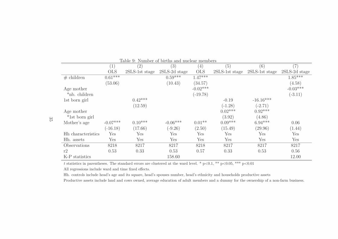
Table 9: Number of births and nuclear members(1) (2) (3) (4) (5) (6) (7)


(53.06) (10.43) (34.57) (4.58)Age mother -0.02*** -0.03***


(12.59) (-1.28) (-2.71)Age mother 0.02*** 0.92***

*1st born girl (3.92) (4.86)Mother’s age -0.07*** 0.10*** -0.06*** 0.01** 0.09*** 6.94*** 0.06

(-16.18) (17.66) (-9.26) (2.50) (15.49) (29.96) (1.44)Hh characteristics Yes Yes Yes Yes Yes Yes YesHh. assets Yes Yes Yes Yes Yes Yes YesObservations 8218 8217 8217 8218 8217 8217 8217r2 0.53 0.33 0.53 0.57 0.33 0.53 0.56K-P statistics 158.60 12.00





35

Table 10: Number of births and non-nuclear members(1) (2) (3) (4) (5) (6) (7)

OLS 2SLS-1st stage 2SLS-2d stage OLS 2SLS-1st stage 2SLS-1st stage 2SLS-2d stage# children -0.07*** -0.25*** -0.33*** 3.43***

(-5.77) (-3.18) (-5.41) (3.21)Age mother 0.01*** -0.10***

*nb. children (4.46) (-3.49)1st born girl 0.42*** -0.19 -16.16***

(12.59) (-1.28) (-2.71)Age mother 0.02*** 0.92***

*1st born girl (3.92) (4.86)Mother’s age 0.03*** 0.10*** 0.04*** 0.00 0.09*** 6.94*** 0.40***

(4.99) (17.66) (4.31) (0.37) (15.49) (29.96) (3.93)Hh characteristics Yes Yes Yes Yes Yes Yes YesHh. assets Yes Yes Yes Yes Yes Yes YesObservations 8218 8217 8217 8218 8217 8217 8217r2 0.13 0.33 0.10 0.13 0.33 0.53 -0.78K-P statistics 158.60 12.00





36

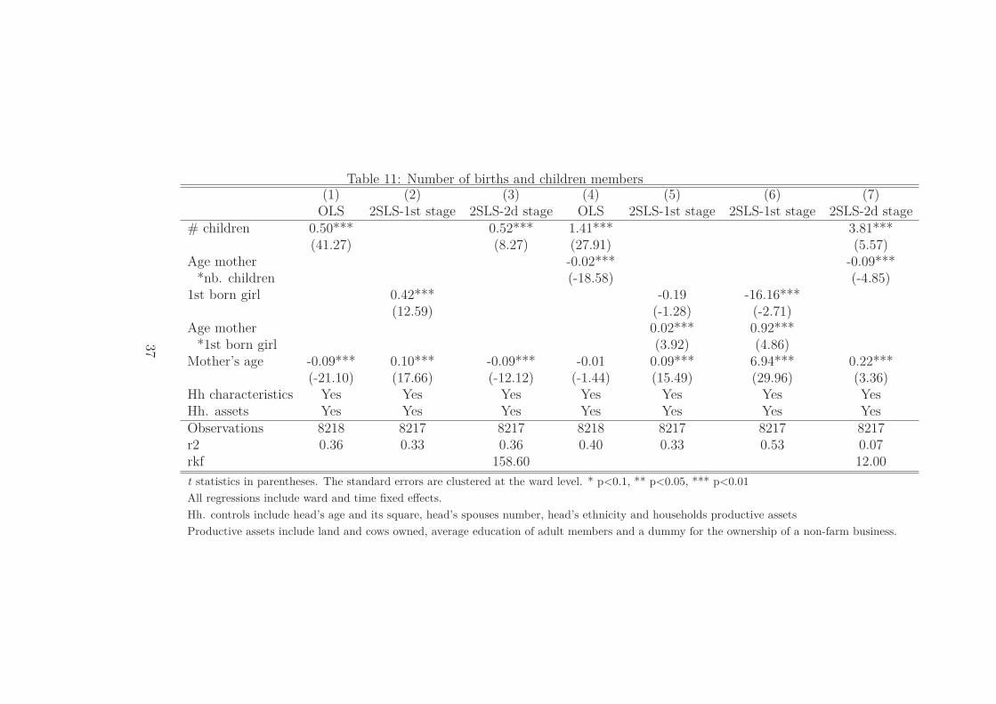
Table 11: Number of births and children members(1) (2) (3) (4) (5) (6) (7)


(41.27) (8.27) (27.91) (5.57)Age mother -0.02*** -0.09***


(12.59) (-1.28) (-2.71)Age mother 0.02*** 0.92***

*1st born girl (3.92) (4.86)Mother’s age -0.09*** 0.10*** -0.09*** -0.01 0.09*** 6.94*** 0.22***

(-21.10) (17.66) (-12.12) (-1.44) (15.49) (29.96) (3.36)Hh characteristics Yes Yes Yes Yes Yes Yes YesHh. assets Yes Yes Yes Yes Yes Yes YesObservations 8218 8217 8217 8218 8217 8217 8217r2 0.36 0.33 0.36 0.40 0.33 0.53 0.07rkf 158.60 12.00





37

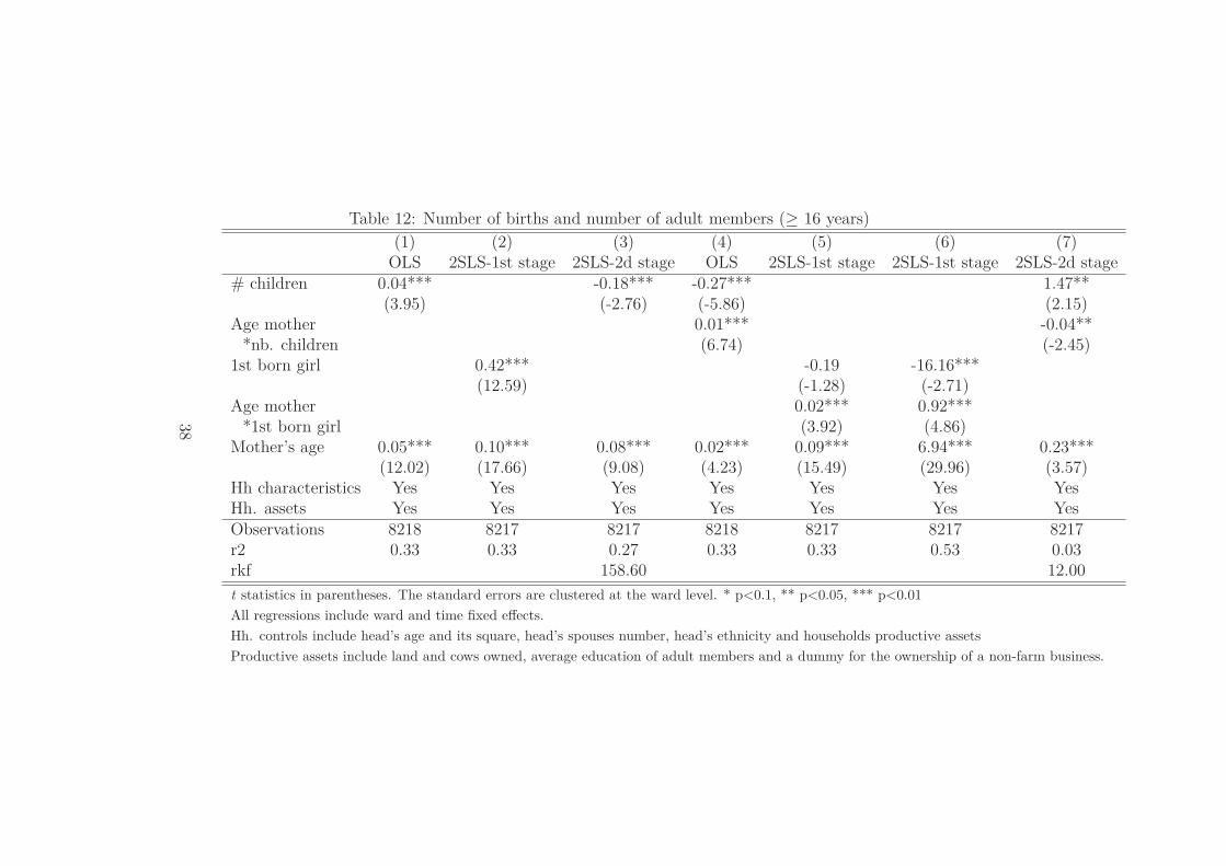
Table 12: Number of births and number of adult members (≥ 16 years)


# children 0.04*** -0.18*** -0.27*** 1.47**(3.95) (-2.76) (-5.86) (2.15)

Age mother 0.01*** -0.04***nb. children (6.74) (-2.45)

1st born girl 0.42*** -0.19 -16.16***(12.59) (-1.28) (-2.71)


Mother’s age 0.05*** 0.10*** 0.08*** 0.02*** 0.09*** 6.94*** 0.23***(12.02) (17.66) (9.08) (4.23) (15.49) (29.96) (3.57)

Hh characteristics Yes Yes Yes Yes Yes Yes YesHh. assets Yes Yes Yes Yes Yes Yes YesObservations 8218 8217 8217 8218 8217 8217 8217r2 0.33 0.33 0.27 0.33 0.33 0.53 0.03rkf 158.60 12.00





38

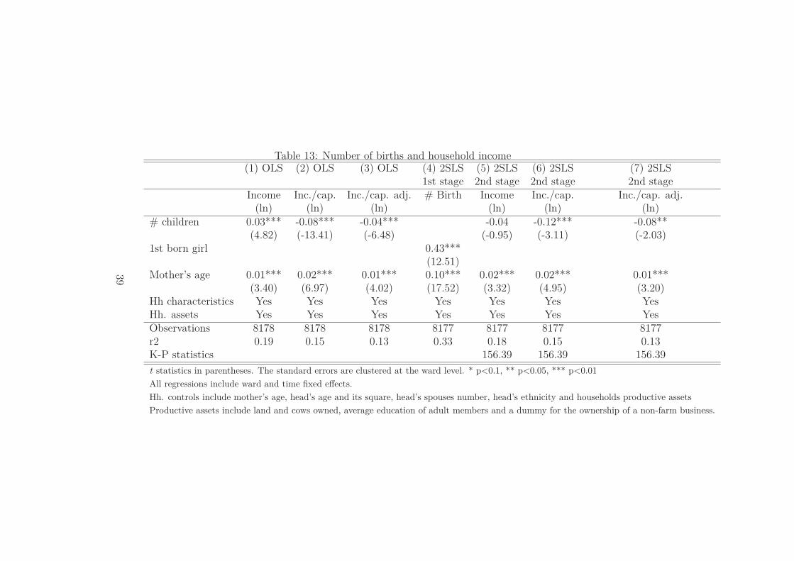
Table 13: Number of births and household income(1) OLS (2) OLS (3) OLS (4) 2SLS (5) 2SLS (6) 2SLS (7) 2SLS

1st stage 2nd stage 2nd stage 2nd stageIncome Inc./cap. Inc./cap. adj. # Birth Income Inc./cap. Inc./cap. adj.

(ln) (ln) (ln) (ln) (ln) (ln)# children 0.03*** -0.08*** -0.04*** -0.04 -0.12*** -0.08**

(4.82) (-13.41) (-6.48) (-0.95) (-3.11) (-2.03)1st born girl 0.43***

(12.51)Mother’s age 0.01*** 0.02*** 0.01*** 0.10*** 0.02*** 0.02*** 0.01***

(3.40) (6.97) (4.02) (17.52) (3.32) (4.95) (3.20)Hh characteristics Yes Yes Yes Yes Yes Yes YesHh. assets Yes Yes Yes Yes Yes Yes YesObservations 8178 8178 8178 8177 8177 8177 8177r2 0.19 0.15 0.13 0.33 0.18 0.15 0.13K-P statistics 156.39 156.39 156.39



Hh. controls include mother’s age, head’s age and its square, head’s spouses number, head’s ethnicity and households productive assets


39

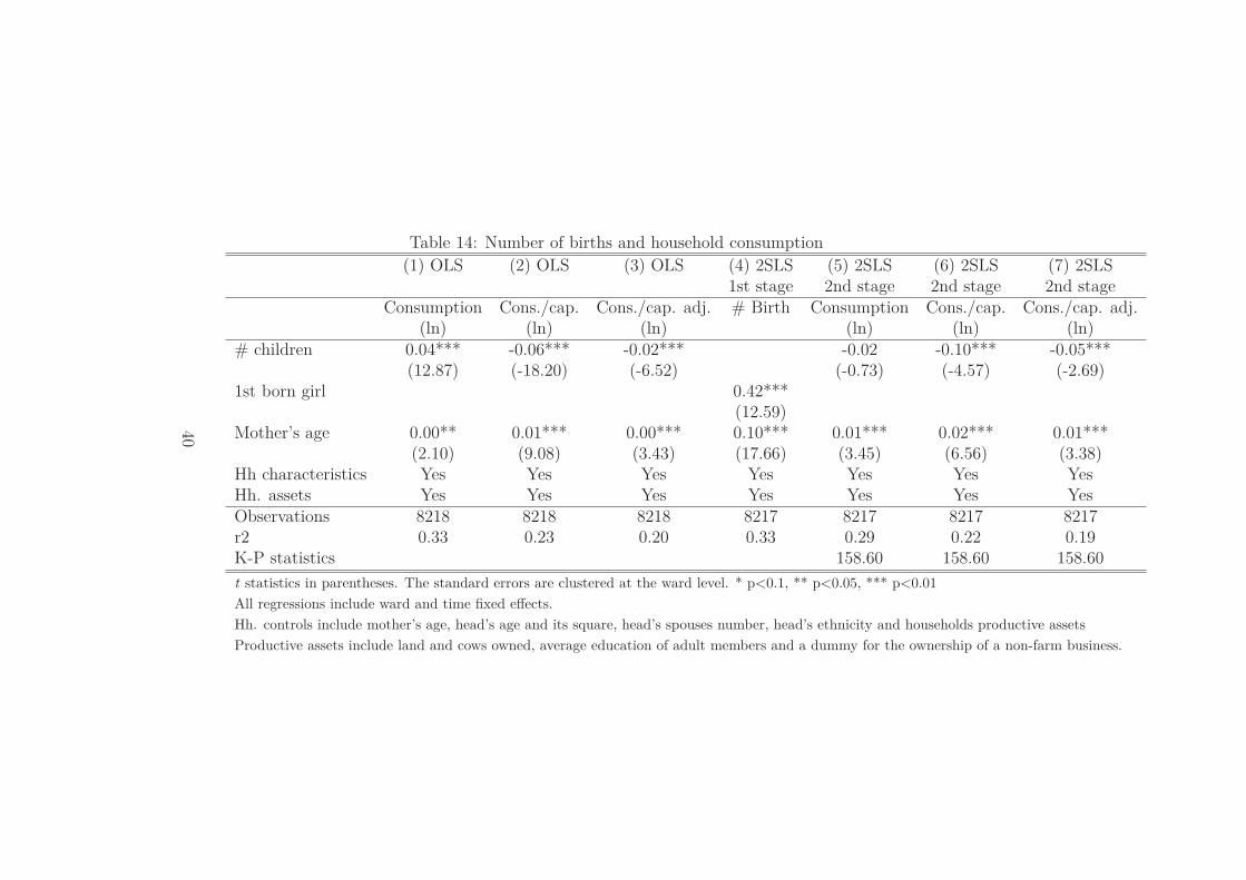
Table 14: Number of births and household consumption

(1) OLS (2) OLS (3) OLS (4) 2SLS (5) 2SLS (6) 2SLS (7) 2SLS1st stage 2nd stage 2nd stage 2nd stage

Consumption Cons./cap. Cons./cap. adj. # Birth Consumption Cons./cap. Cons./cap. adj.(ln) (ln) (ln) (ln) (ln) (ln)

# children 0.04*** -0.06*** -0.02*** -0.02 -0.10*** -0.05***(12.87) (-18.20) (-6.52) (-0.73) (-4.57) (-2.69)

1st born girl 0.42***(12.59)

Mother’s age 0.00** 0.01*** 0.00*** 0.10*** 0.01*** 0.02*** 0.01***(2.10) (9.08) (3.43) (17.66) (3.45) (6.56) (3.38)

Hh characteristics Yes Yes Yes Yes Yes Yes YesHh. assets Yes Yes Yes Yes Yes Yes YesObservations 8218 8218 8218 8217 8217 8217 8217r2 0.33 0.23 0.20 0.33 0.29 0.22 0.19K-P statistics 158.60 158.60 158.60





40

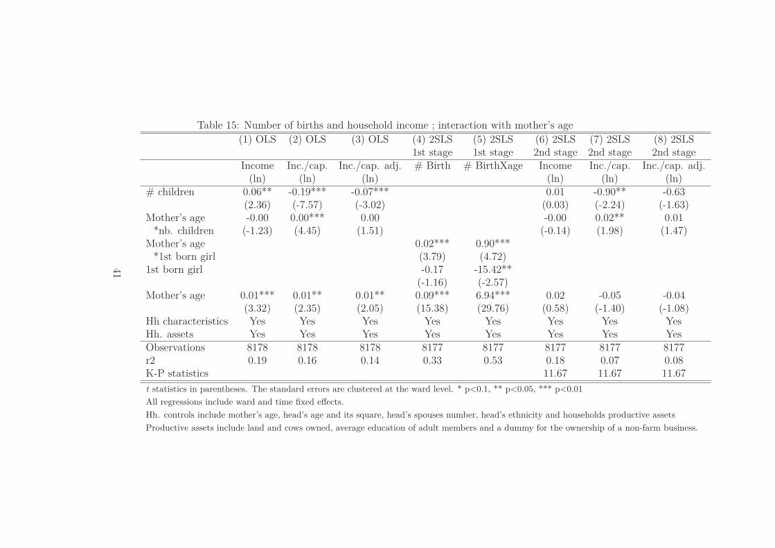
Table 15: Number of births and household income ; interaction with mother’s age

(1) OLS (2) OLS (3) OLS (4) 2SLS (5) 2SLS (6) 2SLS (7) 2SLS (8) 2SLS1st stage 1st stage 2nd stage 2nd stage 2nd stage

Income Inc./cap. Inc./cap. adj. # Birth # BirthXage Income Inc./cap. Inc./cap. adj.(ln) (ln) (ln) (ln) (ln) (ln)

# children 0.06** -0.19*** -0.07*** 0.01 -0.90** -0.63(2.36) (-7.57) (-3.02) (0.03) (-2.24) (-1.63)

Mother’s age -0.00 0.00*** 0.00 -0.00 0.02** 0.01*nb. children (-1.23) (4.45) (1.51) (-0.14) (1.98) (1.47)

Mother’s age 0.02*** 0.90****1st born girl (3.79) (4.72)

1st born girl -0.17 -15.42**(-1.16) (-2.57)

Mother’s age 0.01*** 0.01** 0.01** 0.09*** 6.94*** 0.02 -0.05 -0.04(3.32) (2.35) (2.05) (15.38) (29.76) (0.58) (-1.40) (-1.08)

Hh characteristics Yes Yes Yes Yes Yes Yes Yes YesHh. assets Yes Yes Yes Yes Yes Yes Yes YesObservations 8178 8178 8178 8177 8177 8177 8177 8177r2 0.19 0.16 0.14 0.33 0.53 0.18 0.07 0.08K-P statistics 11.67 11.67 11.67





41

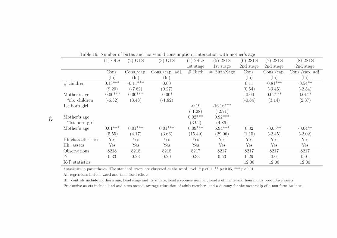
Table 16: Number of births and household consumption ; interaction with mother’s age

(1) OLS (2) OLS (3) OLS (4) 2SLS (5) 2SLS (6) 2SLS (7) 2SLS (8) 2SLS1st stage 1st stage 2nd stage 2nd stage 2nd stage

Cons. Cons./cap. Cons./cap. adj. # Birth # BirthXage Cons. Cons./cap. Cons./cap. adj.(ln) (ln) (ln) (ln) (ln) (ln)

# children 0.13*** -0.11*** 0.00 0.11 -0.81*** -0.54**(9.20) (-7.62) (0.27) (0.54) (-3.45) (-2.54)

Mother’s age -0.00*** 0.00*** -0.00* -0.00 0.02*** 0.01***nb. children (-6.32) (3.48) (-1.82) (-0.64) (3.14) (2.37)

1st born girl -0.19 -16.16***(-1.28) (-2.71)

Mother’s age 0.02*** 0.92****1st born girl (3.92) (4.86)

Mother’s age 0.01*** 0.01*** 0.01*** 0.09*** 6.94*** 0.02 -0.05** -0.04**(5.55) (4.17) (3.66) (15.49) (29.96) (1.15) (-2.45) (-2.02)

Hh characteristics Yes Yes Yes Yes Yes Yes Yes YesHh. assets Yes Yes Yes Yes Yes Yes Yes YesObservations 8218 8218 8218 8217 8217 8217 8217 8217r2 0.33 0.23 0.20 0.33 0.53 0.29 -0.04 0.01K-P statistics 12.00 12.00 12.00





42

A APPENDIX

43

Table A.1: The age of the household’s head and the composition of the households

Head’s age # Households Pr.(nuclear hh.) Size of Hh. # Births Spouse Child Grand-child

< 31 1627 0.66 4.49 2.32 0.70 2.13 0.0031 ≤ . ≤ 40 3197 0.71 5.24 3.45 0.79 2.88 0.0241 ≤ . ≤ 50 2574 0.61 5.50 4.24 0.87 2.77 0.2451 ≤ . ≤ 60 742 0.54 5.76 4.56 1.01 2.69 0.4661 ≤ 78 0.67 5.42 4.58 1.00 2.56 0.42All sample 8218 0.65 5.22 3.58 0.82 2.68 0.13

Head’s age Parents Siblings Nephew/niece Child-in-law Sibling-in-law Parent-in-law Others

< 31 0.23 0.18 0.06 0.01 0.04 0.06 0.0731 ≤ . ≤ 40 0.20 0.09 0.09 0.05 0.03 0.04 0.0641 ≤ . ≤ 50 0.15 0.05 0.08 0.23 0.03 0.02 0.0751 ≤ . ≤ 60 0.10 0.03 0.02 0.36 0.02 0.01 0.0661 ≤ 0.01 0.00 0.10 0.26 0.00 0.00 0.06All sample 0.18 0.09 0.07 0.13 0.03 0.04 0.06

44

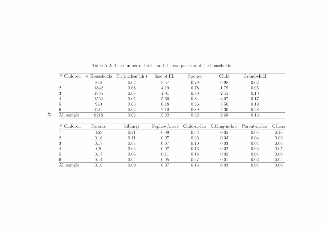
Table A.2: The number of births and the composition of the households

# Children # Households Pr.(nuclear hh.) Size of Hh. Spouse Child Grand-child

1 826 0.62 3.57 0.79 0.98 0.022 1842 0.68 4.19 0.78 1.79 0.053 1835 0.68 4.91 0.80 2.45 0.104 1564 0.65 5.66 0.84 3.07 0.175 940 0.63 6.18 0.86 3.50 0.196 1211 0.62 7.10 0.89 4.36 0.28All sample 8218 0.65 5.22 0.82 2.68 0.13

# Children Parents Siblings Nephew/niece Child-in-law Sibling-in-law Parent-in-law Others

1 0.23 0.21 0.09 0.03 0.05 0.05 0.102 0.18 0.11 0.07 0.06 0.03 0.04 0.093 0.17 0.08 0.07 0.10 0.03 0.04 0.064 0.20 0.06 0.07 0.16 0.02 0.03 0.055 0.17 0.06 0.11 0.18 0.02 0.04 0.066 0.14 0.04 0.05 0.27 0.01 0.02 0.04All sample 0.18 0.09 0.07 0.13 0.03 0.04 0.06

45

Table A.3: Number of births and household composition - second born

(1)OLS (2)OLS (3)OLS (4)2SLS (5)2SLS (6)2SLS (7)2SLS1st stage 2d stage 2d stage 2d stage

Hh. size Nucl. mb. Non-nucl. mb. # children Hh. size Nucl. mb. Non-nucl. mb.# children 0.53*** 0.59*** -0.06*** 0.32*** 0.65*** -0.33***

(28.09) (45.78) (-4.22) (2.97) (9.86) (-3.59)1st born girl -0.10** -0.01 -0.09** 0.43*** -0.01 -0.03 0.03

(-2.24) (-0.27) (-2.52) (12.78) (-0.11) (-0.93) (0.57)2nd born girl 0.37***

(10.92)Hh characteristics Yes Yes Yes Yes Yes Yes YesHh. assets Yes Yes Yes Yes Yes Yes YesObservations 7392 7392 7392 7388 7388 7388 7388r2 0.33 0.48 0.13 0.31 0.31 0.48 0.07K-P statistics 119.27 119.27 119.27





46

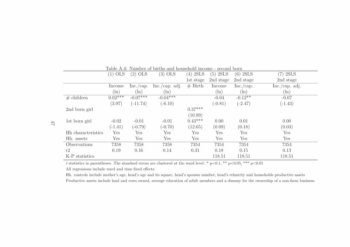
Table A.4: Number of births and household income - second born(1) OLS (2) OLS (3) OLS (4) 2SLS (5) 2SLS (6) 2SLS (7) 2SLS

1st stage 2nd stage 2nd stage 2nd stageIncome Inc./cap. Inc./cap. adj. # Birth Income Inc./cap. Inc./cap. adj.

(ln) (ln) (ln) (ln) (ln) (ln)# children 0.02*** -0.07*** -0.04*** -0.04 -0.12** -0.07

(3.97) (-11.74) (-6.10) (-0.81) (-2.47) (-1.43)2nd born girl 0.37***

(10.89)1st born girl -0.02 -0.01 -0.01 0.43*** 0.00 0.01 0.00

(-1.41) (-0.79) (-0.70) (12.65) (0.09) (0.18) (0.03)Hh characteristics Yes Yes Yes Yes Yes Yes YesHh. assets Yes Yes Yes Yes Yes Yes YesObservations 7358 7358 7358 7354 7354 7354 7354r2 0.19 0.16 0.14 0.31 0.18 0.15 0.13K-P statistics 118.51 118.51 118.51





47

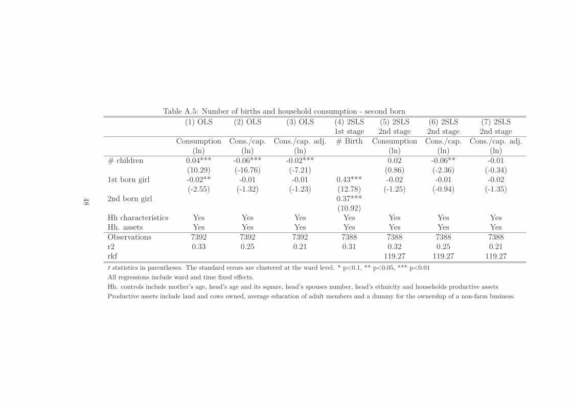
Table A.5: Number of births and household consumption - second born

(1) OLS (2) OLS (3) OLS (4) 2SLS (5) 2SLS (6) 2SLS (7) 2SLS1st stage 2nd stage 2nd stage 2nd stage

Consumption Cons./cap. Cons./cap. adj. # Birth Consumption Cons./cap. Cons./cap. adj.(ln) (ln) (ln) (ln) (ln) (ln)

# children 0.04*** -0.06*** -0.02*** 0.02 -0.06** -0.01(10.29) (-16.76) (-7.21) (0.86) (-2.36) (-0.34)

1st born girl -0.02** -0.01 -0.01 0.43*** -0.02 -0.01 -0.02(-2.55) (-1.32) (-1.23) (12.78) (-1.25) (-0.94) (-1.35)

2nd born girl 0.37***(10.92)

Hh characteristics Yes Yes Yes Yes Yes Yes YesHh. assets Yes Yes Yes Yes Yes Yes YesObservations 7392 7392 7392 7388 7388 7388 7388r2 0.33 0.25 0.21 0.31 0.32 0.25 0.21rkf 119.27 119.27 119.27





48

Table A.6: Number of births and children-in-law(1) (2) (3) (4) (5) (6) (7)

OLS 2SLS-1st stage 2SLS-2d stage OLS 2SLS-1st stage 2SLS-1st stage 2SLS-2d stage# children -0.00 -0.16*** -0.12*** 1.06***

(-1.24) (-6.78) (-7.56) (3.14)Age mother 0.00*** -0.03***


(12.53) (-1.40) (-2.77)Age mother 0.02*** 0.93***

*1st boorn girl (4.03) (4.92)Mother’s age 0.02*** 0.10*** 0.03*** 0.01*** 0.09*** 6.93*** 0.15***

(11.06) (17.58) (10.24) (2.84) (15.40) (29.80) (4.35)Hh characteristics Yes Yes Yes Yes Yes Yes YesHh. assets Yes Yes Yes Yes Yes Yes YesObservations 8218 8217 8217 8218 8217 8217 8217r2 0.14 0.33 -0.19 0.15 0.33 0.53 -1.63rkf 157.09 10.98





49

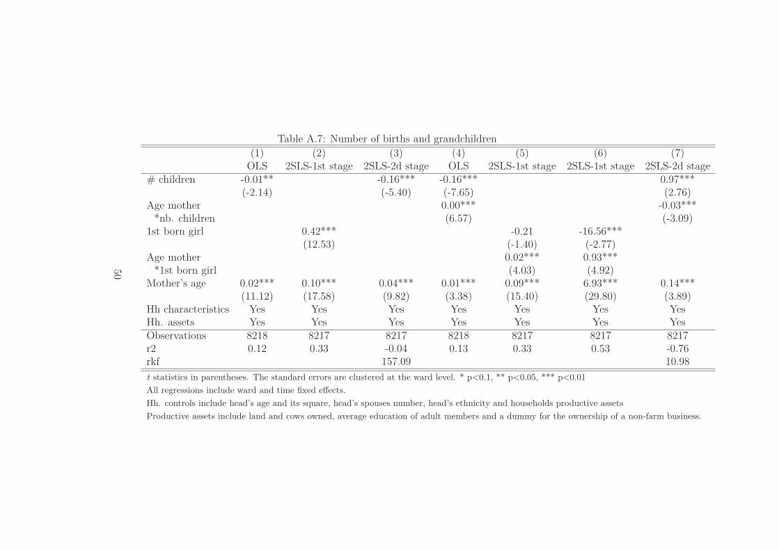
Table A.7: Number of births and grandchildren


# children -0.01** -0.16*** -0.16*** 0.97***(-2.14) (-5.40) (-7.65) (2.76)

Age mother 0.00*** -0.03****nb. children (6.57) (-3.09)

1st born girl 0.42*** -0.21 -16.56***(12.53) (-1.40) (-2.77)


Mother’s age 0.02*** 0.10*** 0.04*** 0.01*** 0.09*** 6.93*** 0.14***(11.12) (17.58) (9.82) (3.38) (15.40) (29.80) (3.89)

Hh characteristics Yes Yes Yes Yes Yes Yes YesHh. assets Yes Yes Yes Yes Yes Yes YesObservations 8218 8217 8217 8218 8217 8217 8217r2 0.12 0.33 -0.04 0.13 0.33 0.53 -0.76rkf 157.09 10.98





50

Table A.8: Number of births and Parents and parents-in-law


# children -0.01*** 0.04 -0.01 0.29(-3.94) (1.59) (-0.38) (1.08)

Age mother -0.00 -0.01*nb. children (-0.42) (-0.97)

1st born girl 0.42*** -0.21 -16.56***(12.53) (-1.40) (-2.77)


Mother’s age -0.00 0.10*** -0.01** -0.00 0.09*** 6.93*** 0.02(-0.97) (17.58) (-2.30) (-0.37) (15.40) (29.80) (0.72)

Hh characteristics Yes Yes Yes Yes Yes Yes YesHh. assets Yes Yes Yes Yes Yes Yes YesObservations 8218 8217 8217 8218 8217 8217 8217r2 0.10 0.33 0.07 0.10 0.33 0.53 0.05rkf 157.09 10.98





51

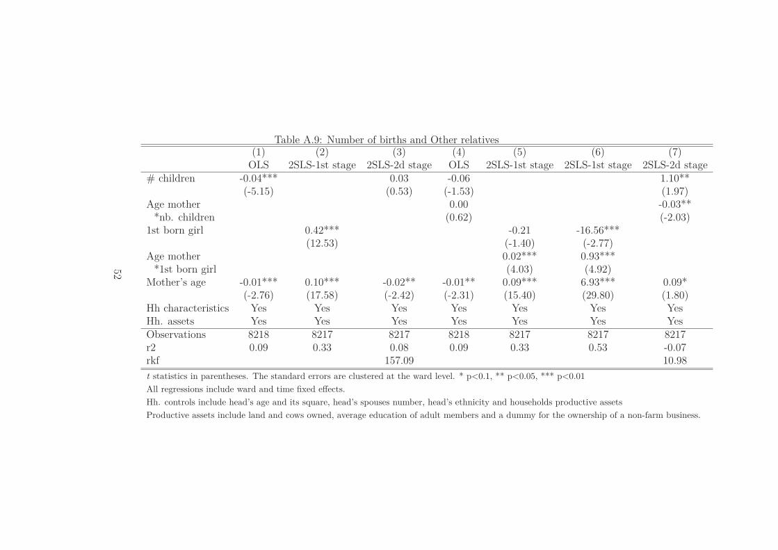
Table A.9: Number of births and Other relatives(1) (2) (3) (4) (5) (6) (7)

OLS 2SLS-1st stage 2SLS-2d stage OLS 2SLS-1st stage 2SLS-1st stage 2SLS-2d stage# children -0.04*** 0.03 -0.06 1.10**

(-5.15) (0.53) (-1.53) (1.97)Age mother 0.00 -0.03**


(12.53) (-1.40) (-2.77)Age mother 0.02*** 0.93***

*1st born girl (4.03) (4.92)Mother’s age -0.01*** 0.10*** -0.02** -0.01** 0.09*** 6.93*** 0.09*

(-2.76) (17.58) (-2.42) (-2.31) (15.40) (29.80) (1.80)Hh characteristics Yes Yes Yes Yes Yes Yes YesHh. assets Yes Yes Yes Yes Yes Yes YesObservations 8218 8217 8217 8218 8217 8217 8217r2 0.09 0.33 0.08 0.09 0.33 0.53 -0.07rkf 157.09 10.98





52

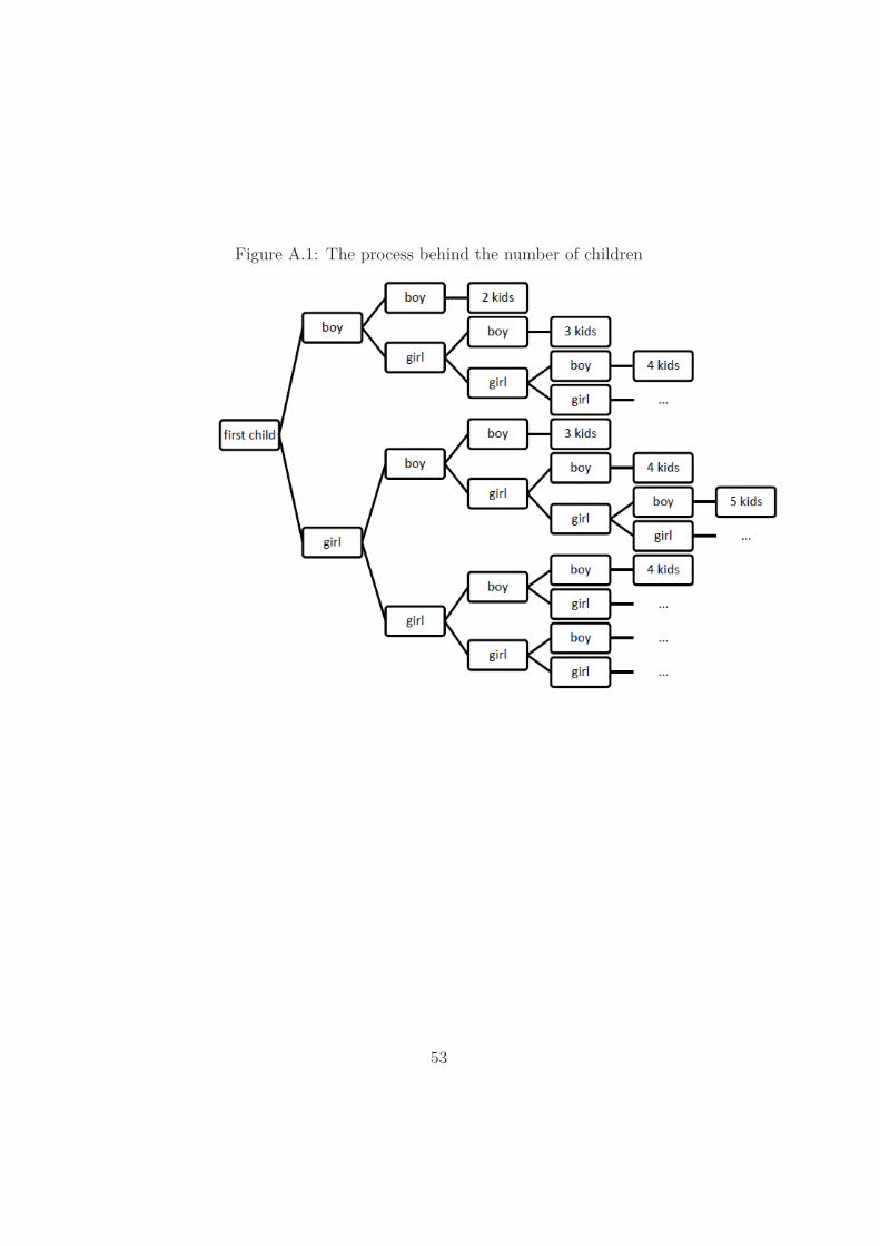
Figure A.1: The process behind the number of children

53

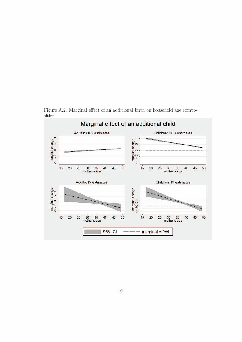
Figure A.2: Marginal effect of an additional birth on household age compo-sition

54

Figure A.3: Marginal effect of an additional birth on parents and otherrelatives presence

55

Documents

Fertility, Household’s size and Poverty in Nepal · PDF fileFertility, Household’s size and Poverty in Nepal * ... Those who contest this view generally argue that ... between