Embed Size (px)
Citation preview

Select/Special Topics from ‘Theory of Atomic Collisions and Spectroscopy’
PCD STiTACS Unit 4
Feynman Diagram Methods 1
P. C. Deshmukh
Department of Physics
Indian Institute of Technology Madras
Chennai 600036
Unit 4 Lecture Number 25
Feynman Diagram Methods
Schrodinger, Heisenberg and Dirac ‘pictures’
Primary references: [1] Fetter and Walecka – Quantum Theory of Many-Particle Systems [2] Raimes – Many Electron Theory

2 PCD STiTACS Unit 4 Feynman Diagram Methods
2
HF-SCF :
2.21 0.916
s s
HF
FEG in jellium potential
Rydr r
E
N
: Bohr unitssr
Average HF energy
per electron
0
4
2
2
2
1 13.60569... 2
1 0.5292... A
meRyd eV
Bohr unitme
Second (and higher) Order Perturbative treatment of the
electron-electron Coulomb interaction however diverges.
electron-electron interaction, reduces the energy BELOW that of
the Sommerfeld gas (of course in the positive jellium potential)
First Order Perturbative treatment of the exchange term SAME RESULT
STiTACS Unit 3 (RPA);
L19, L20; Slides # 96, 97

3 PCD STiTACS Unit 4 Feynman Diagram Methods
Bohm & Pines: mid-fiftees
D.Pines (1963) Elementary excitations in solids (Benjamin, NY)
2 42
322
2.21 0.916 3 0.916
2 482
cBP
s s s fs
kE
r r r kr
2
:
2.21 0.916
s s
HF
For free electron gas in jellium potential
Rydr r
E
N
Random Phase Approximation
Need!
Many-body
theory – beyond perturbation
methods
kc : Upper bound to wave number of plasma oscillations
Lower bound to wave length; since oscillations get
damped by the random thermal motion of the electrons.

4 PCD STiTACS Unit 4 Feynman Diagram Methods
‘Exact
Solution’ ? “Having no body at all is already too many”
– G. E. Brown
( ) ( ) ( ) ( )
1 1 1( ,.., ) ( ,.., ) ( ,.., )N N N N
N N NH q q q q E q q
2
( )
1 1
1
2
N NiN
i i ji ij
i ZH
m r r
Many
electron
problem
Non – Perturbative Methods / eg. RPA
Alternative techniques:
Configuration interaction methods:
Multi-Configuration Hartree-Fock (MCHF)
Multi-Configuration Dirac-Hartree-Fock (MCDHF)
Feynman Diagram
Methods

5 PCD STiTACS Unit 4 Feynman Diagram Methods
The above Hamiltonian
not an explicit function of time
If we can treat this term as if it has a time-
dependence, then the mathematical procedure
that would enables us to do so, would also
provide access to powerful methods using the
INTERACTION (Dirac) “PICTURE”.
2
( )
1 1
1
2
N NiN
i i ji ij
i ZH
m r r
6 PCD STiTACS Unit 4 Feynman Diagram Methods
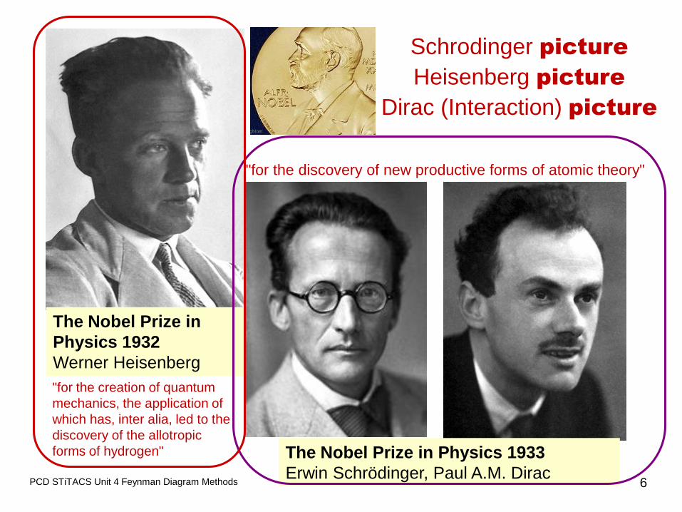
The Nobel Prize in Physics 1933
Erwin Schrödinger, Paul A.M. Dirac
The Nobel Prize in
Physics 1932
Werner Heisenberg
"for the creation of quantum
mechanics, the application of
which has, inter alia, led to the
discovery of the allotropic
forms of hydrogen"
"for the discovery of new productive forms of atomic theory"
Schrodinger picture
Heisenberg picture
Dirac (Interaction) picture

7 PCD STiTACS Unit 4 Feynman Diagram Methods
Schrodinger picture
Heisenberg picture
Dirac (Interaction) picture
‘picture’
‘representation’
, ,H r t i r tt
time-evolution: , ,0 Hi t
r t re
, ,0 Ei t
r t re
2 31 1
1 ......2! 3!
Hi t H H Hi t i t i te
,0 ,0H r E r stationary states
Time dependent wave
function
Schrodinger picture

8 PCD STiTACS Unit 4 Feynman Diagram Methods
, ,0 Ei t
r t re
State functions are
TIME DEPENDENT
, , INDEPENDENT
of time
OPERATORS q p H
Schrödinger picture
, ,S SH r t i r tt
Schrödinger equation in the
Schrödinger picture PCD STiTACS Unit 4 Feynman Diagram Methods

9 PCD STiTACS Unit 4 Feynman Diagram Methods
UNITARY TRANSFORMATIONS
- leave the ‘physics’ invariant…..
-Rotation of basis in the Hilbert space
-‘Generalized’ rotations from one ‘picture’ to ‘another’
† ; H H
i t i t
O e O e
, ,0H r t r
time independent…
wavefunction at t=0
H H
i t i t
H Se e
Heisenberg Picture
( )
( )
H
H
fn time
fn time

10 PCD STiTACS Unit 4 Feynman Diagram Methods
UNITARY TRANSFORMATIONS
- leave the ‘physics’ invariant…..
-Rotation of basis in the Hilbert space
-‘Generalized’ rotations from one ‘picture’ to ‘another’ † ;
H Hi t i t
O e O e
, , , H
i t
H H S Sr t O r t e r t
, ,0 E
S S
i tr t re
, ,0 ,0 H E
i t
H
i tr t e r re
, ,0H r t r
time independent…
wavefunction at t=0
H H
i t i t
H Se e
but ( )H H H St H H fn t
Heisenberg Picture
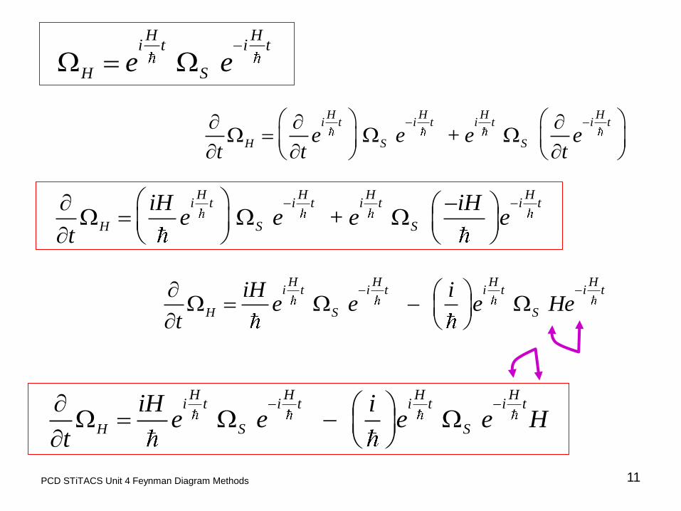
11 PCD STiTACS Unit 4 Feynman Diagram Methods
H H
i t i t
H Se e
+ H H H H
i t i t i t i t
H S Se e e et t t
+ H H H H
i t i t i t i t
H S S
iH iHe e e e
t
H H H H
i t i t i t i t
H S S
iH ie e e He
t
H H H H
i t i t i t i t
H S S
iH ie e e e H
t
,H H
iH
t
, H Hi Ht
12 PCD STiTACS Unit 4 Feynman Diagram Methods
H H
i t i t
H Se e
H H H H
i t i t i t i t
H S S
iH ie e e e H
t
H H H
iH iH
t
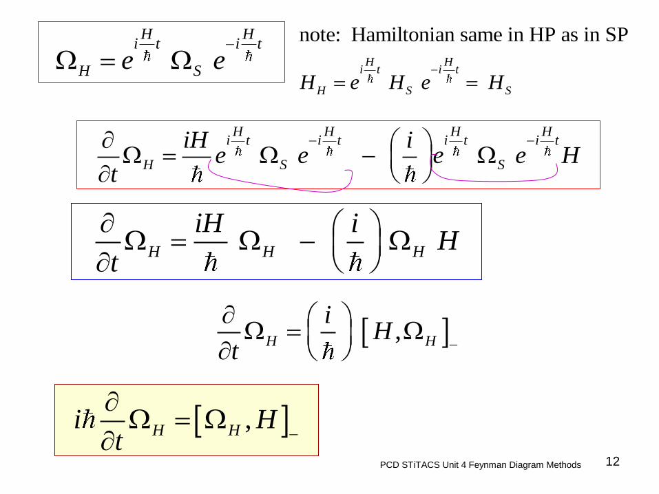
note: Hamiltonian same in HP as in SP
H H
i t i t
H S SH e H e H

13 PCD STiTACS Unit 4 Feynman Diagram Methods
UNITARY TRANSFORMATIONS
Hi t
O e
H H
i t i t
H Se e
Heisenberg Picture
( )
( )
H
H
fn time
fn time
Dirac Picture
Interaction
Picture
0 1H H H
, , H
i t
H Sr t e r t
0 0 0
& , , H H H
i t i t i t
I S I Se e r t e r t
I IBOTH and are functions of time
( )
( , ) ( )
S
S
fn time
r t fn time
Schrodinger Picture
oHi t
O e

14 PCD STiTACS Unit 4 Feynman Diagram Methods
0 1H H H
0 0
0
( )
, ,
H Hi t i t
I S
Hi t
I S
t e e
r t e r t
oHi t
O e
, ,S SH r t i r tt
Schrodinger equation
0
0 1 , , H
i t
S IH H r t i e r tt
0
, , H
i t
I Se r t r t
Unitary transformation
operator that effects
transformation to the
Dirac/Interaction picture
↑
Soluble part

15 PCD STiTACS Unit 4 Feynman Diagram Methods
0
0 1, , , H
i t
S S IH r t H r t i e r tt
0
, , H
i t
I Sr t e r t
0
0 1 0, , , + ,H
i t
S S S IH r t H r t H r t i e r tt
0 0
00 1, , , + ,
H Hi t i t
S S I I
HH r t H r t i i e r t i e r t
t
0
0 1 , , H
i t
S IH H r t i e r tt

16 PCD STiTACS Unit 4 Feynman Diagram Methods
0 0
1 , ,H H
i t i t
I IH e r t i e r tt
( ) , ,I I IH t r t i r tt
0
, ,H
i t
S Ir t e r t
0
1 , ,H
i t
S IH r t i e r tt
, ,H r t i r tt
Schrodinger equation
00
1 , ,H
i ti
I
H
I
t
H e r t i re tt
Just “like”
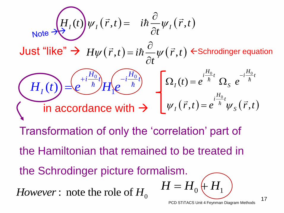
17 PCD STiTACS Unit 4 Feynman Diagram Methods
( ) , ,I I IH t r t i r tt
, ,H r t i r tt
Schrodinger equation Just “like”
0 0
1( ) H H
i t i t
IH t e H e
0 0
0
( )
, ,
H Hi t i t
I S
Hi t
I S
t e e
r t e r t
in accordance with
Transformation of only the ‘correlation’ part of
the Hamiltonian that remained to be treated in
the Schrodinger picture formalism.
0 1H H H 0: note the role of However H

The subscript I denotes the transformation
to the INTERACTION PICTURE of the
difficult/correlation part of the
Hamiltonian.
18 PCD STiTACS Unit 4 Feynman Diagram Methods
0 0
1( ) H H
i t i t
IH t e H e
0 1H H H
Notation
1H

19 PCD STiTACS Unit 4 Feynman Diagram Methods
0 0
1( ) H H
i t i t
IH t e H e
Transformation of only the ‘correlation’ part of
the Hamiltonian that remained to be treated in
the Schrodinger picture formalism.
0 1H H H
( ) , ,I I IH t r t i r tt
0 0
0
( )
, ,
H Hi t i t
I S
Hi t
I S
t e e
r t e r t
0 1
, ( )
is determined
I r t fn time
Time dependence by both H and H
20 PCD STiTACS Unit 4 Feynman Diagram Methods
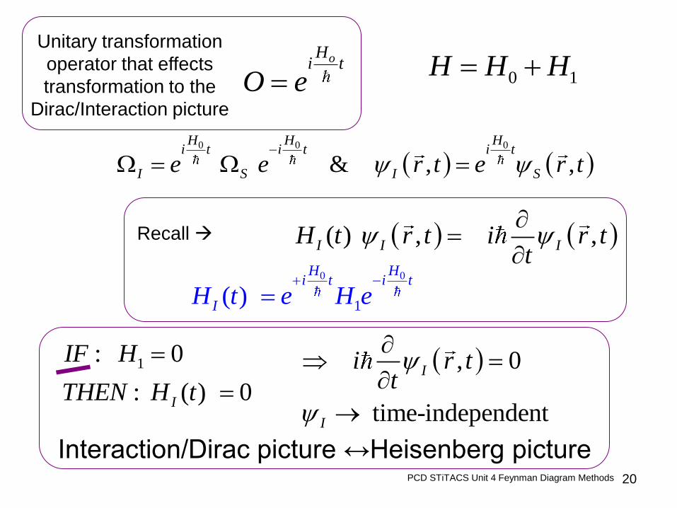
0 0 0
& , , H H H
i t i t i t
I S I Se e r t e r t
oHi t
O e
Unitary transformation
operator that effects
transformation to the
Dirac/Interaction picture
0 1H H H
( ) , ,I I IH t r t i r tt
0 0
1( ) H H
i t i t
IH t e H e
Recall
1: 0
: ( ) 0I
IF H
THEN H t
, 0
time-independent
I
I
i r tt
Interaction/Dirac picture ↔Heisenberg picture

1 1 0 0, ,I It U t t U t t t
21 PCD STiTACS Unit 4 Feynman Diagram Methods
0
,
Time Development Operator
U t t
0 0,I It U t t t
,I It U t t t
1 3 1 2 2 3
, 1
, , ,
U t t
U t t U t t U t t
Reference: Fetter and Walecka –
Quantum Theory of Many-Particle Systems,
Chapter 3
FW/Eq.6.11/page 55
0 0
1
0 0
1 , , ,
, ,
U t t U t t U t t
U t t U t t
Existence of UNIT operator
Closure property
Existence of INVERSE
‘GROUP’ properties

22 PCD STiTACS Unit 4 Feynman Diagram Methods
0 0,I It U t t t
†
0 0
† 1
0 0
, , 1
, ,
U t t U t t
U t t U t t unitary
†
0 0 0 0, ,I I I It t t U t t U t t t
norm 0 0I I I It t t t
23 PCD STiTACS Unit 4 Feynman Diagram Methods
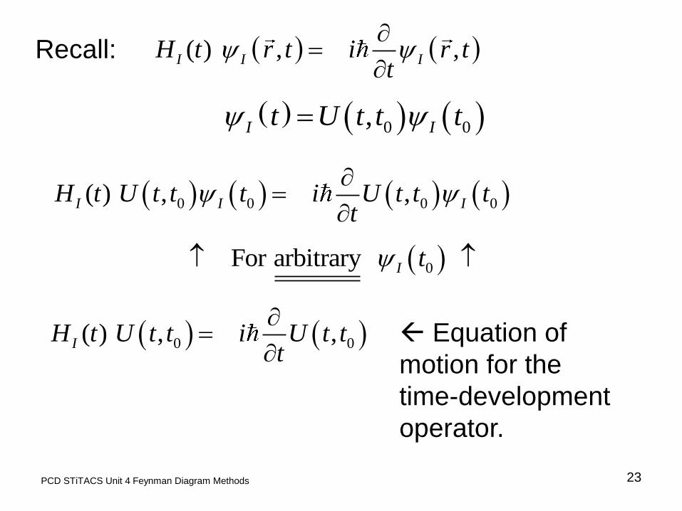
( ) , ,I I IH t r t i r tt
Recall:
0 0,I It U t t t
0 0 0 0( ) , ,I I IH t U t t t i U t t tt
0 For arbitrary I t
0 0( ) , ,IH t U t t i U t tt
Equation of
motion for the
time-development
operator.

PCD STiTACS Unit 4 Feynman Diagram Methods 24
0 0 0
& , , H H H
i t i t i t
I S I Se e r t e r t
time-evolution of Schrodinger state:
, ,0 Hi t
r t re
0
0 0 : , , H
t tiIf initial time is t r t r te
0 0
0
0, , ,H H H
i t i t i t t
I S Sr t e r t e e r t

0 0
0
0, , ,H H H
i t i t i t t
I S Sr t e r t e e r t
0
0
0 0, ,H
i t
S Ir t e r t
0 0
0 0
0, ,H HH
i t i t t i t
I Ir t e e e r t
0 0
0 0
0, H HH
i t i t t i t
U t t e e e
Time Evolution: t0 to t
PCD STiTACS Unit 4 Feynman Diagram Methods 25

26 PCD STiTACS Unit 4 Feynman Diagram Methods
0 0
0 0
0, H HH
i t i t t i t
U t t e e e
† † †AB B A
0 0
0 0†
0, H HH
i t i t t i t
U t t e e e
† 1
0 0, ,U t t U t t
27 PCD STiTACS Unit 4 Feynman Diagram Methods Questions: [email protected]
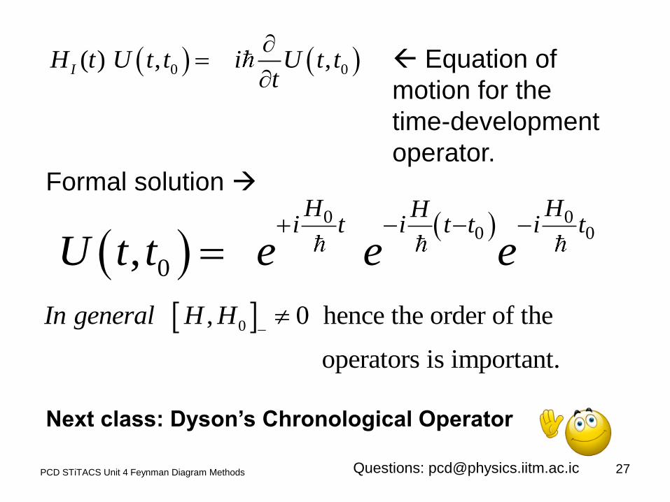
0 0( ) , ,IH t U t t i U t tt
Equation of
motion for the
time-development
operator.
0 0
0 0
0, H HH
i t i t t i t
U t t e e e
Formal solution
0 , 0 hence the order of the
operators is important.
In general H H
Next class: Dyson’s Chronological Operator

Select/Special Topics from ‘Theory of Atomic Collisions and Spectroscopy’
28
P. C. Deshmukh
Department of Physics
Indian Institute of Technology Madras
Chennai 600036
PCD STiTACS Unit 4 Feynman Diagram Methods
Unit 4 Lecture Number 26
Feynman Diagram Methods
Dyson’s Chronological Operator
Primary references: Fetter and Walecka – Quantum Theory of Many-Particle Systems Raimes – Many Electron Theory

29 PCD STiTACS Unit 4 Feynman Diagram Methods
0 0( ) , ,IH t U t t i U t tt
0 0
0 0
0, H HH
i t i t t i t
U t t e e e
Equation of
motion for the
time-development
operator. Formal solution
Today:
we develop an integral equation for the time
development operator
0 0, , ,I Ir t U t t r t
I
I I
I Time evolution
of interaction
picture states
Differential equation for the
Time Evolution Operator

30 PCD STiTACS Unit 4 Feynman Diagram Methods
, ' '( ) , ' ( ) , 'I Ii U t t H t U t t H t U t tt
Raimes
– Many Electron Theory
Eq.5.32 page 97
Fetter and Walecka
– Quantum Theory of Many Particle Systems
Eq.6.17, page 56
0 0, ( ) , Ii U t t H t U t tt

31
0 0, ( ) , Ii U t t H t U t tt
0 0i.e. , ( ) , I
iU t t H t U t t
t
0 0
0 0' ', ' ( ') ', '
t t
It t
idt U t t dt H t U t t
t
0 integrating from to : t t
0
0 0 0 0 , , ' ( ') ', t
It
iU t t U t t dt H t U t t
0
0 0 , =1 ' ( ') ', t
It
iU t t dt H t U t t
0 0 , 1 U t t
PCD STiTACS Unit 4 Feynman Diagram Methods

We are dealing with operators….
….so we must preserve the ‘ordering’ 32 PCD STiTACS Unit 4 Feynman Diagram Methods
0 , time development operators
not ordinary functions of time t
U t t
0
0 0 , =1 ' ( ') ', t
It
iU t t dt H t U t t
Independent variable t appears as UPPER LIMIT
If U were ordinary functions, then such integrals
would be “VOLTERRA INTEGRALS”
Iterative solutions available; which are guaranteed to converge in the case of ordinary functions …… …… we attempt similar procedures in the present case.

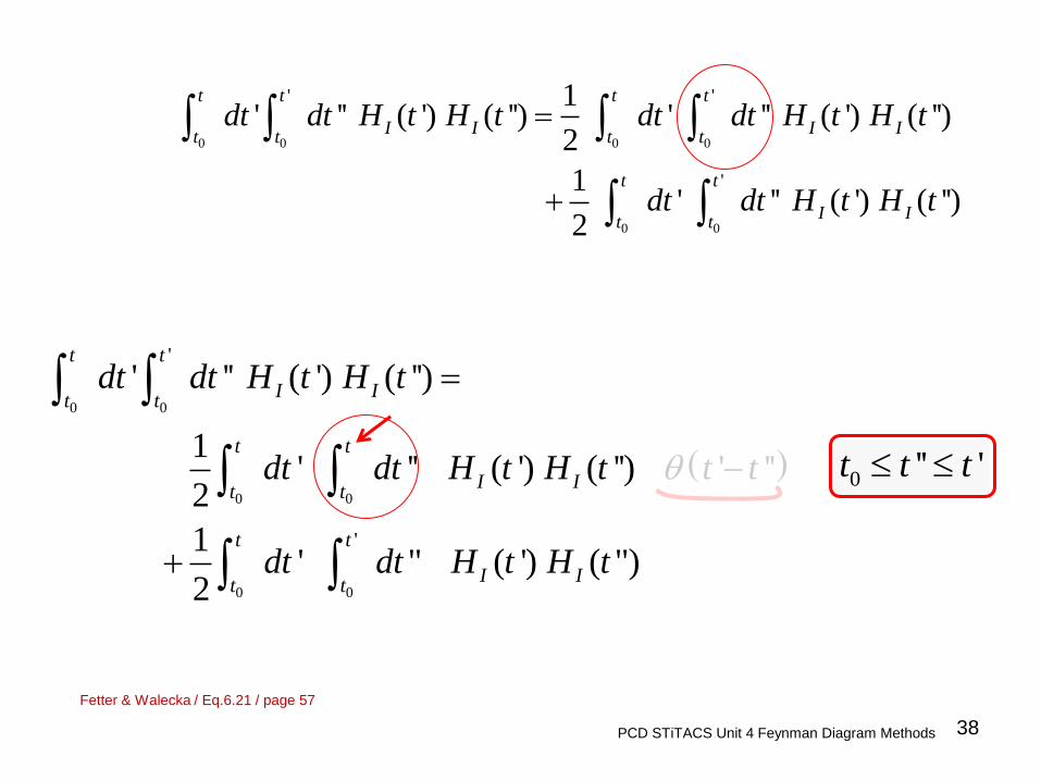
33 PCD STiTACS Unit 4 Feynman Diagram Methods
0
0 0 , =1 ' ( ') ', t
It
iU t t dt H t U t t
0
'
0 0 ', =1 '' ( '') '', t
It
iU t t dt H t U t t
0 0
'
0 0 , =1 ' ( ') 1 '' ( '') '', t t
I It t
i iU t t dt H t dt H t U t t
0 0 0
2'
0 0, =1 ' ( ') ' ( ') '' ( '') '', t t t
I I It t t
i iU t t dt H t dt H t dt H t U t t
0 0 0
2'
0 0, =1 ' ( ') ' '' ( ') ( '') '', t t t
I I It t t
i iU t t dt H t dt dt H t H t U t t
Order of the operators is important: left ↓right↓

34 PCD STiTACS Unit 4 Feynman Diagram Methods
0 0 0
2'
0 0, =1 ' ( ') ' '' ( ') ( '') '', t t t
I I It t t
i iU t t dt H t dt dt H t H t U t t
0 0 0
2'
0, =1 ' ( ') ' '' ( ') ( '') .... t t t
I I It t t
i iU t t dt H t dt dt H t H t
0
''
0 0 '', =1 ''' ( ''') ''', t
It
iU t t dt H t U t t
0 0 0 0
0 0
' '
'
1' '' ( ') ( '') ' '' ( ') ( '')
2
1 ' '' ( ') ( '')
2
t t t t
I I I It t t t
t t
I It t
dt dt H t H t dt dt H t H t
dt dt H t H t
Consider the 3rd term

35
''t
't
' ''t t
0t
PCD STiTACS Unit 4 Feynman Diagram Methods
0
0
'
''
t t t
t t t
0t
'' 't t
' ''t t
0 0 0 0
0 0
' '
'
1' '' ( ') ( '') ' '' ( ') ( '')
2
1 ' '' ( ') ( '')
2
t t t t
I I I It t t t
t t
I It t
dt dt H t H t dt dt H t H t
dt dt H t H t
''t t
't t
Fetter & Walecka / Fig.6.1 / page 57
Raimes / Fig.5.1/page 100
Integration is over the variables t’ and t’’

36
''t
't
' ''t t
0t
PCD STiTACS Unit 4 Feynman Diagram Methods
0
0
'
''
t t t
t t t
0t
'' 't t
' ''t t
0 0 0 0
0 0
' '
'
1' '' ( ') ( '') ' '' ( ') ( '')
2
1 ' '' ( ') ( '')
2
t t t t
I I I It t t t
t t
I It t
dt dt H t H t dt dt H t H t
dt dt H t H t
''t t
't tFetter & Walecka / Fig.6.1 / page 57
Raimes / Fig.5.1/page 100
Integration is over the variables t’ and t’’

37 PCD STiTACS Unit 4 Feynman Diagram Methods
x
x
cx x
( ) 1cx x
Heaviside
step function
; 0
; 1
c
c
x x x
x x x
0 0 0 0
0 0
' '
'
1' '' ( ') ( '') ' '' ( ') ( '')
2
1 ' '' ( ') ( '')
2
t t t t
I I I It t t t
t t
I It t
dt dt H t H t dt dt H t H t
dt dt H t H t
38 PCD STiTACS Unit 4 Feynman Diagram Methods
0 0
0 0
0 0
'
'
' '' ( ') ( '')
1 ' '' ( ') ( '') ' ''
2
1 ' " ( ') ( ")
2
t t
I It t
t t
I It t
t t
I It t
dt dt H t H t
dt dt H t H t t t
dt dt H t H t
0 '' 't t t
Fetter & Walecka / Eq.6.21 / page 57

0 0 0 0
0 0
'
'
1' '' ( ') ( '') ' '' ( ') ( '') ' ''
2
1 ' " ( ') ( ")
2
t t t t
I I I It t t t
t t
I It t
dt dt H t H t dt dt H t H t t t
dt dt H t H t
0 0
0 0
0 0
'
' '' ( ') ( '')
1 ' '' ( ') ( '') ' ''
2
1 '' ' ( '') ( ') '' '
2
t t
I It t
t t
I It t
t t
I It t
dt dt H t H t
dt dt H t H t t t
dt dt H t H t t t
39 PCD STiTACS Unit 4 Feynman Diagram Methods
0 0
0 0
0 0
'
' '' ( ') ( '')
1 ' '' ( ') ( '') ' ''
2
1 ' " ( ') ( ") ' "
2
t t
I It t
t t
I It t
t t
I It t
dt dt H t H t
dt dt H t H t t t
dt dt H t H t t t
0 '' 't t t
Fetter & Walecka
Eq.6.21 / page 57
nd
'' '
in 2 term
t t

40 PCD STiTACS Unit 4 Feynman Diagram Methods
0 0
0 0
0 0
'
' '' ( ') ( '')
1 ' '' ( ') ( '') ' ''
2
1 '' ' ( '') ( ') '' '
2
t t
I It t
t t
I It t
t t
I It t
dt dt H t H t
dt dt H t H t t t
dt dt H t H t t t
Operators containing the latest time stand farthest to the left.
0 0
0 0
'
' '' ( ') ( '')
1' '' ( ') ( '') ' '' ( '') (
2') '' 'I I
t t
I It t
t t
t tI IH t H t t
dt dt H t H
t H t H t t t
t
dt dt
Fetter & Walecka / Eq.6.21 / page 57
Combining the two terms:

0 0
0 0
'
' '' ( ') ( '')
1' '' ( ') ( '') ' '' ( '') (
2') '' 'I I
t t
I It t
t t
t tI IH t H t t
dt dt H t H
t H t H t t t
t
dt dt
41
PCD STiTACS Unit 4 Feynman Diagram Methods
Operators containing the latest time stand farthest to the left.
0 0 0 0
' 1' '' ( ') ( '') ' ''
2( ') ( '')
t t t t
It
I IIt t t
dt dt H t H t dt dt H tT H t
T: Time-ordered product of operators. Operators containing the latest time stand farthest to the left.
Fetter & Walecka / Eq.6.21 / page 57
Fetter & Walecka / Eq.6.22 / page 58
0 0 0
2'
0, =1 ' ( ') ' '' ( ') ( '') .... t t t
I I It t t
i iU t t dt H t dt dt H t H t
0 0 0
0 1 2
0
1 2(1
, = . ). !
( ).. ( )
nt t
I It
It
n
n
t
nt
H t H t Hi
U t t dt dt dtn
tT
Fetter & Walecka / Eq.6.23 / page 58
Generalizing:
Fetter & Walecka / Eq.6.19 / page 57
1 2 ! ' - ' , ,....., nThere are n time orderings of the time labels t t t

T: Time-ordered product of operators. Operators containing the latest time stand farthest to the left.
0 0 0
2'
0, =1 ' ( ') ' '' ( ') ( '') .... t t t
I I It t t
i iU t t dt H t dt dt H t H t
Fetter & Walecka / page 57,58
42 PCD STiTACS Unit 4 Feynman Diagram Methods
0 0 0
0 1 2
0
1 2(1
, = . ). !
( ).. ( )
nt t
I It
It
n
n
t
nt
H t H t Hi
U t t dt dt dtn
tT
2
'
, =1 ' ( ') ' '' ( ') ( '') .... t t t
I I I
i iU t dt H t dt dt H t H t
1 21 2
0
( ) ( ).. ( )1
, = .. !
nt t t
I n
n
I InTi
U t dt dt d H t H t tt Hn
0Now, let t
1
, =1 with n
n
U t U
1 2 1 2
1 .. ( ) ( ).. ( )
!
nt t t
n n I I I n
iU dt dt dt T H t H t H t
n

43 PCD STiTACS Unit 4 Feynman Diagram Methods
1 2 1 2 1 2
2 1 2 1
if
if
T A t B t A t B t t t
B t A t t t
1 2 1 2 1 2
2 1
if
I I I I
I I
T H t H t H t H t t t
H t H t
1 2 1 2 1 2
2 1 2 1
if
if
I I I I
I I
T H t H t H t H t t t
H t H t t t
1 2 : chronologically same! t t
T: Time-ordered product of operators. Operators containing the latest time stand farthest to the left.
1 2 2 1
I I I IT H t H t T H t H t

44 PCD STiTACS Unit 4 Feynman Diagram Methods
0 0 0
0 1 2 1 2
0
1, = .. ( ) ( ).. ( )
!
nt t t
n I I I nt t t
n
iU t t dt dt dt T H t H t H t
n
Consider nth term in this series:
0 0 0
1 2 1 2
1 .. ( ) ( ).. ( )
!
nt t t
n I I I nt t t
idt dt dt T H t H t H t
n
1 2
! ' - '
, ,....., n
There are n time orderings of the time labels
t t t
1 2 one of these n! ways is: ....... nt t t
1 2
1 1
, ,..., are dummy labels that get integrated out
and
( ) .. ( ).. ( ).. ( ) ( ) .. ( ).. ( ).. ( )
n
I I i I j I n I I j I i I n
t t t
T H t H t H t H t T H t H t H t H t
T: Time-ordered product of operators. Operators containing the latest time stand farthest to the left.
i↓ j↓ i↓ j↓

0 1 0; + full Hamiltonianas t H H H
45 PCD STiTACS Unit 4 Feynman Diagram Methods
0 1H H H Perturbation: ‘unfriendly’ part
‘solvable’ part
ADIABATIC “SWITCHING” of the PERTURBATION
0 1
tH H e H
: small (positive) ; in the end 0
0 ; 0 & soluble parttas t e H H
Perturbation is turned on and off very slowly
quasi-static (adiabatic) ;
end-results to be obtained independent of α.
Raimes – Many Electron Theory Eq.6.6 page 105
adiabatic switching
control parameter

46 PCD STiTACS Unit 4 Feynman Diagram Methods
0 1
tH H e H This mathematical device enables us use the
provisions of the INTERACTION PICTURE
very fruitfully.
adiabatic switching
control parameter
0 1 0; + full Hamiltonianas t H H H
: small (positive) ; in the end 0
0 ; 0 & soluble parttas t e H H
47 PCD STiTACS Unit 4 Feynman Diagram Methods
0 1
tH H e H
INTERACTION PICTURE
0 0 0
, , H H H
i t i t i t
I S I Se e r t e r t
0 0
1 H H
i t i tt
IH t e e H e
0 0
1( ) H H
i t i t
IH t e H e
Perturbation: ‘unfriendly’ part,
controlled by the mathematical switch
adiabatic switching
control parameter
48 PCD STiTACS Unit 4 Feynman Diagram Methods
0 0, ( ) , Ii U t t H t U t tt
0 0 0
0 1 2 1 2
0
1, = .. ( ) ( ).. ( )
!
nt t t
n I I I nt t t
n
iU t t dt dt dt T H t H t H t
n
0 0
1 H H
i t i tt
IH e e H e
(1)
(2)
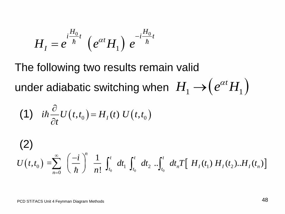
The following two results remain valid
under adiabatic switching when 1 1
tH e H

The time development operator must explicitly depend on α
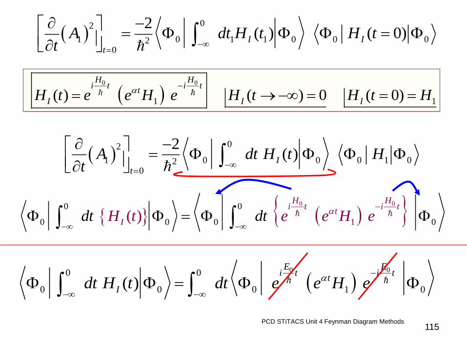
49 PCD STiTACS Unit 4 Feynman Diagram Methods
0 0,I It U t t t
0 0( ) , ,IH t U t t i U t tt
Interaction
picture
0 0,I It U t t t
0 0
0
, ,
H Hi t i t
I S
Hi t
I S
e e
r t e r t
0 0 0
0 1 2 1 2
0
1, = .. ( ) ( ).. ( )
!
nt t t
n I I I nt t t
n
iU t t dt dt dt T H t H t H t
n
0 0 0
0
1 2 1 2
0
, =
1= .. ( ) ( ).. ( )
!
nt t t
n I I I nt t t
n
U t t
idt dt dt T H t H t H t
n
0 1
tH H e H
0 1H H H
0 0
1 H H
i t i tt
IH e e H e
0
00
, ,0 HH
S H H
i t i tr t r re e
50 PCD STiTACS Unit 4 Feynman Diagram Methods
0 0 0 0
0 0
:
H E
time independent stationary eigenstate of H
Time evolution of the Schrodinger state if there
were no ‘correlations’
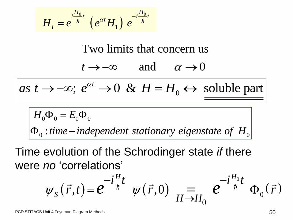
0 ; 0 & soluble parttas t e H H
Two limits that concern us
and 0t
0 0
1 H H
i t i tt
IH e e H e
51 PCD STiTACS Unit 4 Feynman Diagram Methods
0
00
time-evolution: , ,0 HH
S H H
i t i tr t r re e
0 0
0 0
If there were NO correlations, , would evolve as:
, independent of time
I
H Hi t
I
i t
r t
r t e r re
0 1 0 t
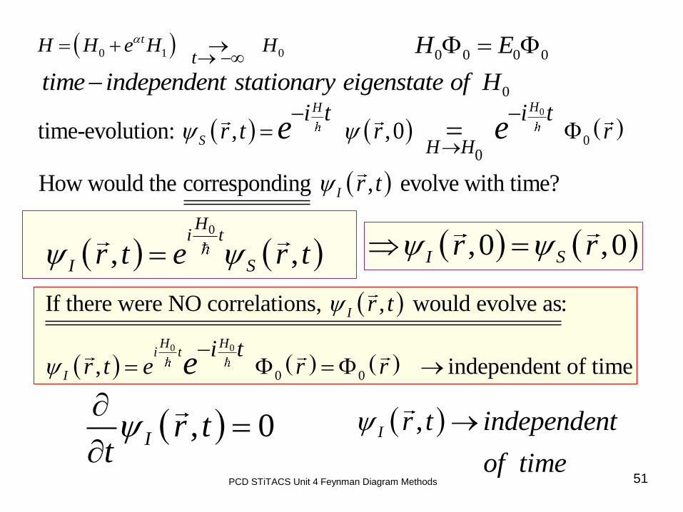
tH H e H H
, 0I r tt
0 0 0 0 H E
0 time independent stationary eigenstate of H
How would the corresponding , evolve with time?I r t
0
, , H
i t
I Sr t e r t
,
I r t independent
of time
,0 ,0I Sr r

52 PCD STiTACS Unit 4 Feynman Diagram Methods
The eigenstates of H0 remain independent of
time in the interaction picture;
since in this case the perturbation H1=0.
0 1
,
t
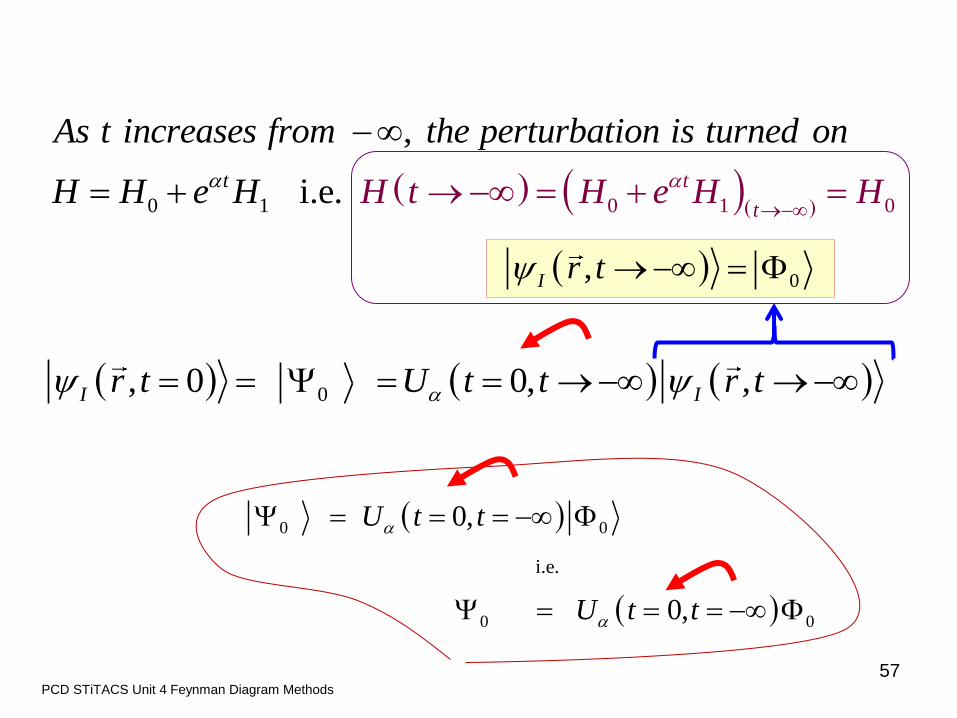
As t increases from the perturbation is turned on
H H e H
0 0,I It U t t t
0 0
0 0
If there were NO correlations, , would evolve as:
, independent of time
I
H Hi t
I
i t
r t
r t e r re
When correlation is present

53 PCD STiTACS Unit 4 Feynman Diagram Methods
Next class:
What happens in the limit α→0?
Gell-Mann and Low theorem
Questions: [email protected]
Two limits that concerned us: & 0t
0 1
0
t
t
H H e H
H H
0,I r t
0
0
, 0
0, ,
0,
I
I
r t
U t t r t
U t t

Select/Special Topics from ‘Theory of Atomic Collisions and Spectroscopy’
54
P. C. Deshmukh
Department of Physics
Indian Institute of Technology Madras
Chennai 600036
PCD STiTACS Unit 4 Feynman Diagram Methods
Unit 4 Lecture Number 27
Feynman Diagram Methods
Gell-Mann and Low Theorem M. Gell-Mann and F. Low Phys.Rev. 84:350 (1951)

0 0 , 0 0, I r t U t t
0 0 0
, , H H H
i t i t i t
I S I Se e r t e r t
, , H H H
i t i t i t
H S H Se e r t e r t
0 1
tH H e H
, 0
, 0
, 0
, 0
, 0 , 0
H
H
S
S
I
I
r tr t
r t
r
t r
t
r
, ,0 E
S S
i tr t re
Schrodinger picture
0 0 0 0H r E r
55
0 0 ; , St
H H r r
Dirac / Interaction picture
Heisenberg picture

PCD STiTACS Unit 4 Feynman Diagram Methods
56
1: 0
: ( ) 0I
IF H
THEN H t
, 0
time-independent
I
I
i r tt
Interaction/Dirac picture ↔Heisenberg picture
0 0 0
, , H H H
i t i t i t
I S I Se e r t e r t
, , H H H
i t i t i t
H S H Se e r t e r t
0 1
tH H e H
0
0
1 0 =0, H=H & , ,0
, , = ,0
Ei t
S S
Hi t
I S S
If H r t e r
r t e r t r
PCD STiTACS Unit 4 Feynman Diagram Methods
57
1 00 1 0
,
i.e. t
t
t
As t increases from the perturbation is tur
H t H
ned
e
on
H e H HH H
0 , I r t
0, 0 0, ,I Ir t U t t r t
0 0
0 0
i.e.
0,
0,
U t t
U t t

58 PCD STiTACS Unit 4 Feynman Diagram Methods
Today,
we examine the following question:
What happens in the limit α→0?
Gell-Mann and Low theorem
Two limits concern us: (1) & (2) 0 t
0 1 0
0
;
: full Hamiltonian (with correlations)
t
t
tH H e H H H
H
Fetter & Walecka,
Quantum Theory of Many-Particle Systems
pages 60, 61
0
0 0
, 0 0, ,
0,
I Ir t U t t r t
U t t

0 0
00 0 0 0
0 1
0 0
0 00 0
(0, ) lim ,
(0, )
;
. .
UIf exists
U
then it is an eigenstate of H H H
i e H E
59 PCD STiTACS Unit 4 Feynman Diagram Methods
Gell-Mann and Low theorem
For ‘PROOF’, see:
Fetter & Walecka
Quantum Theory of
Many-Particle Systems,
page 61
0 1 0 t
tH H e H H
0 0 0 0 H E
Question: 0 1 ?How do we get eigenstate of H H H
0 0 , 0 0, I r t U t t
0 t

from which is an eigen-state of the
unperturbed Hamiltonian:
The eigenstate
60 PCD STiTACS Unit 4 Feynman Diagram Methods
Gell-Mann and Low theorem
0 1 0 t
tH H e H H
0 0 0 0 H E
0 0
00 0 00
(0, )lim
(0, )
U
U
0 1 of H H H develops ADIABETICALLY
0
0 0 0 0 H E
0 0 , 0 0, I r t U t t

61 PCD STiTACS Unit 4 Feynman Diagram Methods
0
, , 0 = , 0
0,
H S Ir t r t r t
U t t
The question we had asked: what happens in the limit α→0?
0 1 0 t
tH H e H H
0 0 0 0 H E
0 0
00 0 00
(0, ) lim
(0, )
U
U
00
lim 0, need not be well defined. U t t
Limit of
the RATIO
0 0 , 0 0, I r t U t t
0 1
0
0 t
tH H e H H

62 PCD STiTACS Unit 4 Feynman Diagram Methods
0 0
00 0 00
(0, )lim
(0, )
U
U
00
lim 0, need not be well defined. U t t
Limit of
the RATIO
The phase of the numerator diverges in
the limit α→0, but it is nicely cancelled
in the ratio by the denominator. Gell-Mann and
Low theorem
0 0 , 0 0, I r t U t t
The question we had asked: what happens in the limit α→0?

63 PCD STiTACS Unit 4 Feynman Diagram Methods
0 0
00 0 0 0
0 1
0 0
0 00 0
(0, ) lim ,
(0, )
;
. .
UIf exists
U
then it is an eigenstate of H H H
i e H E
Gell-Mann and
Low theorem
0 0
0 0
0 00 0
H E
0 0 0 0
0 00 0
HE
0
0 0 , 0 0, I r t U t t

64 PCD STiTACS Unit 4 Feynman Diagram Methods
0 0 0 0
0 00 0
HE
0 0 0 0 1 0 0 0
0 0 00 0 0
+
H HE
0 0 1 0 0 0
0 00 0
H HE
0 0 0 1 0 0 0
0
0 0 00 0 0
+
HE E
0 1 0
0
0 0
HE E
0 0 , 0 0, I r t U t t
0 0 0 0 = H E 0 1 0 t
tH H e H H
From Gellman & Low Theorem:

65 PCD STiTACS Unit 4 Feynman Diagram Methods
0 1 0
0
0 0
HE E
0 0 , 0 0, I r t U t t
0 0 0 0 = H E
0 1 0 t
tH H e H H
0 1 0
0
0 0
0,
0,
H U t tE E
U t t
Fetter & Walecka
Quantum Theory of Many-Particle Systems, Eq.6.45, page 61
Raimes
Many Electron Theory, Eq.6.15, page 105
0lim
Can the energy
correction depend on α?

66 PCD STiTACS Unit 4 Feynman Diagram Methods
0 1 0
00
0 0
0, lim
0,
H U t tE E
U t t
0 0 00 0
log ,limt
E E i U tt
We now show that:
0 0
0 0
0 00 00
0
,
log , ,
lim limt
t
i U tt
i U tt U t
0 0
0 0
0 0
0 00
0
1
, log ,
,
lim limt
t
U ti U t
ti U t
t
Using:

67 PCD STiTACS Unit 4 Feynman Diagram Methods
0 0
0 0
0 00 00
0
,
log , ,
lim limt
t
i U tt
i U tt U t
0 0
0 0
0 00 00
0
, log ,
,lim lim I
tt
H U ti U t
t U t
0 0now: , ( ) , Ii U t t H t U t tt
0 1 0
0 00
0 00 0
0, log , lim
0, lim
t
H U t ti U t
t U t t
0 0 00 0
log ,limt
E E i U tt
Thus:
Raimes / Many Electron Theory / Eq.6.22, page 106
0 1 0
00
0 0
0, but: lim
0,
H U t tE E
U t t

68 PCD STiTACS Unit 4 Feynman Diagram Methods
0 0
0 00 0
H E
0 0 0 0 = H E
0 1 0 t
tH H e H H
0 ?E E E
0 00 0
log ,limAdiabaticHypothesis t
E i U tt
?
RayleighSchrodinger
PerturbationTheory
E
69 PCD STiTACS Unit 4 Feynman Diagram Methods
0
1 2 1 2
0
, =
1= .. ( ) ( ).. ( )
!
nt t t
n I I I n
n
U t t
idt dt dt T H t H t H t
n
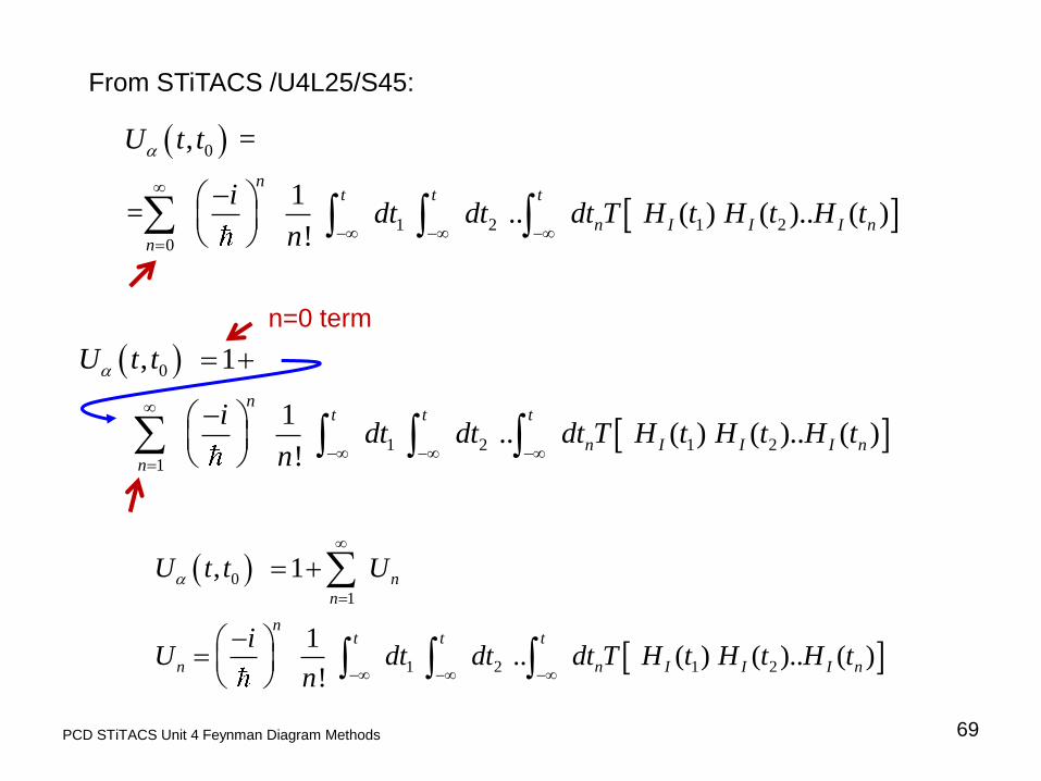
From STiTACS /U4L25/S45:
0
1 2 1 2
1
, 1
1 .. ( ) ( ).. ( )
!
nt t t
n I I I n
n
U t t
idt dt dt T H t H t H t
n
0
1
1 2 1 2
, 1
1 .. ( ) ( ).. ( )
!
n
n
nt t t
n n I I I n
U t t U
iU dt dt dt T H t H t H t
n
n=0 term

70 PCD STiTACS Unit 4 Feynman Diagram Methods
0 00 0
log ,limt
E i U tt
0 0 0 0
1
, 1 n
n
U t U
0
1
1 2 1 2
, 1
1 .. ( ) ( ).. ( )
!
n
n
nt t t
n n I I I n
U t t U
iU dt dt dt T H t H t H t
n
0 0
where
n nA U
1 2
1 1 , ,... . ( ), ( ),... . t t
I Ie e etc appear in H t H t etc
0 1
tH H e H remember that:
0 0
1
1 n
n
U
1
1 n
n
A

71 PCD STiTACS Unit 4 Feynman Diagram Methods
0 0
1
log , log 1 n
n
U t A
0 0
1
, 1 n
n
U t A
0 0 n nA U
2 3 4 51 1 1 1 log 1 ....
2 3 4 5
1 1
e x x x x x x
for x
2 3
0 0
1 1 1
4 5
1 1
1 1log ,
2 3
1 1 ....
4 5
n n n
n n n
n n
n n
U t A A A
A A

72 PCD STiTACS Unit 4 Feynman Diagram Methods
0 00 0
log ,limt
E i U tt
2 3
0 0
1 1 1
4 5
1 1
1 1log ,
2 3
1 1 ....
4 5
n n n
n n n
n n
n n
U t A A A
A A
2 3
1 1 1
4 5
1 1
0
0
1 1
2 3
1 1 ....
4 5
limn n n
n n n
n n
n n t
A A A
E it
A A
0 0
0 1 2 1 2 0
1 .. ( ) ( ).. ( )
!
n n
nt t t
n I I I n
A U
idt dt dt T H t H t H t
n

73 PCD STiTACS Unit 4 Feynman Diagram Methods
2 3
1 1 1
4 5
1 1
0
0
1 1
2 3
1 1 ....
4 5
limn n n
n n n
n n
n n t
A A A
E it
A A
0 0 0 1 2 1 2 0
1 .. ( ) ( ).. ( )
!
nt t t
n n n I I I n
iA U dt dt dt T H t H t H t
n
2 2 2
1 2 3
1 2 3 1 2 1 3 1 4
2 1 2 3 2 4
3 3 3
1 2 3 1 2 3
2 2 2
1 2 1 3 1 4 2 1 3
2 2 2
2 1 2 3 2 4
0
...1
...2
..
... ...1
... ...3
....
lim
A A A
A A A A A A A A A
A A A A A AE i
t A A A A A A
A A A A A A A A A
A A A A A A
0
....
...t
1 2 3 ..E E E E 1
indexed
thn order corrections
by the power of H
Observe where the terms for various orders come from!

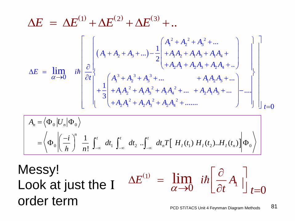
Messy? Let us look at just the I
order term 74 PCD STiTACS Unit 4 Feynman Diagram Methods
1 2 3 ..E E E E
2 2 2
1 2 3
1 2 3 1 2 1 3 1 4
2 1 2 3 2 4
3 3 3
1 2 3 1 2 3
2 2 2
1 2 1 3 1 4 2 1 3
2 2 2
2 1 2 3 2 4
0
...1
...2
..
... ...1
... ...3
....
lim
A A A
A A A A A A A A A
A A A A A AE i
t A A A A A A
A A A A A A A A A
A A A A A A
0
....
...t
0 0
0 1 2 1 2 0
1 .. ( ) ( ).. ( )
!
n n
nt t t
n I I I n
A U
idt dt dt T H t H t H t
n
1
10 0
limt
E i At

75 PCD STiTACS Unit 4 Feynman Diagram Methods
0 0
0 1 2 1 2 0
1 .. ( ) ( ).. ( )
!
n n
nt t t
n I I I n
A U
idt dt dt T H t H t H t
n
1
10 0
limt
E i At
1 0 0
0 1 1 0
( )
n
t
I
A U
idt H t
0 0
1 ( ) H H
i t i t
IH Ht e e
† † †1 v
2i i jj k l
i j i j k l
H c i f j c c c ij lk c c
0 0
H H
i t i t
I Se e
1 1 tH e H
Questions: [email protected]

Select/Special Topics from ‘Theory of Atomic Collisions and Spectroscopy’
76
P. C. Deshmukh
Department of Physics
Indian Institute of Technology Madras
Chennai 600036
PCD STiTACS Unit 4 Feynman Diagram Methods
Unit 4 Lecture Number 28
Feynman Diagram Methods
Correspondence between Adiabatic Switching
technique and Rayleigh-Schrodinger perturbation
theory.

0 0
00 0 0 0
0 1
0 0
0 00 0
(0, ) lim ,
(0, )
;
. .
UIf exists
U
then it is an eigenstate of H H H
i e H E
77 PCD STiTACS Unit 4 Feynman Diagram Methods
Gell-Mann and Low theorem
For ‘PROOF’, see:
Fetter & Walecka
Quantum Theory of
Many-Particle Systems,
page 61
0 1 0 t
tH H e H H
0 0 0 0 H E
Question: 0 1 ?How do we get eigenstate of H H H
0 0 , 0 0, I r t U t t
0 t

78 PCD STiTACS Unit 4 Feynman Diagram Methods
0 0 0 0 = H E 0 1 0 t
tH H e H H
0 ?E E E
From Gellman & Low Theorem:
0 1 0
00
0 0
0, lim
0,
H U t tE E
U t t
0 0 00 0
log ,limAdiabaticHypothesis t
E E E i U tt
We showed that:
?
RayleighSchrodinger
PerturbationTheory
E

79
0 00 0
log ,limt
E i U tt
0 0 0 0
1 1
, 1 1n n
n n
U t U A
0
1
1 2 1 2
, 1
1 .. ( ) ( ).. ( )
!
n
n
nt t t
n n I I I n
U t t U
iU dt dt dt T H t H t H t
n
0 0
where
n nA U
1 2
1 1 , ,... . ( ), ( ),... . t t
I Ie e etc appear in H t H t etc
0 1
tH H e H remember that:
2 3
0 0
1 1 1
4 5
1 1
1 1log ,
2 3
1 1 ....
4 5
n n n
n n n
n n
n n
U t A A A
A A
PCD STiTACS Unit 4 Feynman Diagram Methods

80 PCD STiTACS Unit 4 Feynman Diagram Methods
2 3
1 1 1
4 5
1 1
0
0
1 1
2 3
1 1 ....
4 5
limn n n
n n n
n n
n n t
A A A
E it
A A
0 0 0 1 2 1 2 0
1 .. ( ) ( ).. ( )
!
nt t t
n n n I I I n
iA U dt dt dt T H t H t H t
n
2 2 2
1 2 3
1 2 3 1 2 1 3 1 4
2 1 2 3 2 4
3 3 3
1 2 3 1 2 3
2 2 2
1 2 1 3 1 4 2 1 3
2 2 2
2 1 2 3 2 4
0
...1
...2
..
... ...1
... ...3
....
lim
A A A
A A A A A A A A A
A A A A A AE i
t A A A A A A
A A A A A A A A A
A A A A A A
0
....
...t
1 2 3 ..E E E E 1
indexed
thn order corrections
by the power of H
Observe where the terms for various orders come from!
Messy! Look at just the I
order term 81 PCD STiTACS Unit 4 Feynman Diagram Methods
1 2 3 ..E E E E
2 2 2
1 2 3
1 2 3 1 2 1 3 1 4
2 1 2 3 2 4
3 3 3
1 2 3 1 2 3
2 2 2
1 2 1 3 1 4 2 1 3
2 2 2
2 1 2 3 2 4
0
...1
...2
..
... ...1
... ...3
....
lim
A A A
A A A A A A A A A
A A A A A AE i
t A A A A A A
A A A A A A A A A
A A A A A A
0
....
...t
0 0
0 1 2 1 2 0
1 .. ( ) ( ).. ( )
!
n n
nt t t
n I I I n
A U
idt dt dt T H t H t H t
n
1
10 0
limt
E i At

82 PCD STiTACS Unit 4 Feynman Diagram Methods
0 0
0 1 2 1 2 0
1 .. ( ) ( ).. ( )
!
n n
nt t t
n I I I n
A U
idt dt dt T H t H t H t
n
1
10 0
limt
E i At
1 0 0
0 1 1 0
( )
n
t
I
A U
idt H t
0 0
1 ( ) H H
i t i t
IH Ht e e
† † †1 v
2i i jj k l
i j i j k l
H c i f j c c c ij lk c c
0 0
H H
i t i t
I Se e
1 1 tH e H

83 PCD STiTACS Unit 4 Feynman Diagram Methods
0 0
1 ( ) H H
i t i t
IH Ht e e
† † †1 v
2i i jj k l
i j i j k l
H c i f j c c c ij lk c c
0 0
† i j
H Hi t i t
ece c
Transformation to interaction picture of some
second quantized creation and destruction
operators in some order…..
1 1 tH e H

0 0
† † ( ) ( ) H H
i t i t
i j i je c c e c t c t
84 PCD STiTACS Unit 4 Feynman Diagram Methods
0 0
† i j
H Hi t i t
ece c
0 0 0 0 0 0
† † H H H H H H
i t i t i t i t
j
t
i
t
i
i i
jce e e e e ec c c
0 0
† †
, , ( ) ) (H H
i
i j I i
i t
I j
t
c c c t ce te
suppress subscript I
for ‘interaction picture’
for brevity.

0 0
† † ( ) ( ) H H
i t i t
i j i je c c e c t c t
85 PCD STiTACS Unit 4 Feynman Diagram Methods
0 0
1 ( ) H H
i t i t
IH Ht e e
† †
1
1 v
2 i j k l
i j k l
H c c ij lk c c
0 0 0 0 0 0
† † H H H H H H
i t i t i t i t
j
t
i
t
i
i i
jce e e e e ec c c
† †1 ( ) ( ) ( ) v ( ) ( )
2 i j
t
I k l
i j k l
H t c t c t ij lk c t c t e
0 1 tH H e H
This recipe would work for
any combination of creation
and destruction operators.
α: adiabatic switching:
1 1 tH e H

86 PCD STiTACS Unit 4 Feynman Diagram Methods
† †1 ( ) ( ) ( ) v ( ) ( )
2 i j
t
I k l
i j k l
H t c t c t ij lk c t c t e
,( ) ( ) ?k I kc t c t
0 0
0
, ,
H Hi t i t
I S
Hi t
I S
e e
r t e r t
0 0
,
,
( ) to the equation of motion
( )
I k
H Hi t i t
I k k
c t solution
i c t i e c et t

87 PCD STiTACS Unit 4 Feynman Diagram Methods
0 0
,
,
( ) to the differential equation:
( ) with ( ) ( ) ;
I k
H Hi t i t
I S I I k S k
c t solution
i t i e e t c t ct t
0 0 0 0
0 0 H H H H
i t i t i t i t
S S
H Hi i e e e i e
0 0 0 0
0 0 H H H H
i t i t i t i t
S SH e e e H e
0 0
0,H H
i t i t
Se H e
0,I t H
, , 0( ) ( ),I k I ki c t c t Ht
0 0
0
( ) to the differential equation:
( ) ,
I
H Hi t i t
I S I
t solution
i t i e e t Ht t
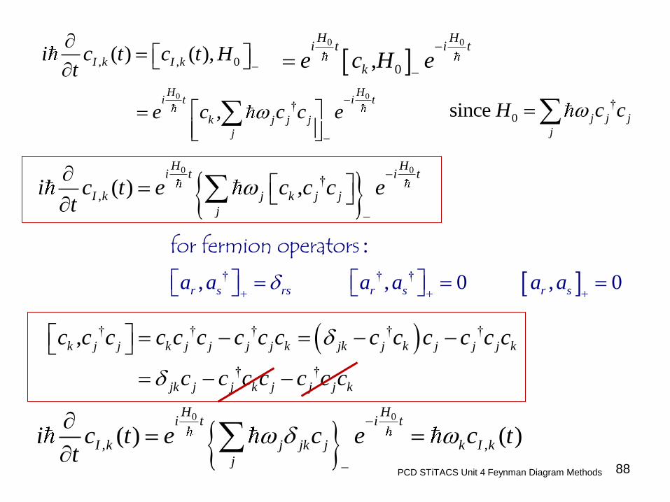
0 0
, ,( ) ( )H H
i t i t
I k j jk j k I k
j
i c t e c e c tt
88 PCD STiTACS Unit 4 Feynman Diagram Methods
, , 0( ) ( ),I k I ki c t c t Ht
0 0
0,H H
i t i t
ke c H e
0 0
†,H H
i t i t
k j j j
j
e c c c e
†
0since j j j
j
H c c
0 0
†
, ( ) ,H H
i t i t
I k j k j j
j
i c t e c c c et
† † †
:
, , 0 , 0r s rs r s r sa a a a a a
for fermion operators
† † † † †
† †
,k j j k j j j j k jk j k j j j k
jk j j k j j j k
c c c c c c c c c c c c c c c
c c c c c c c
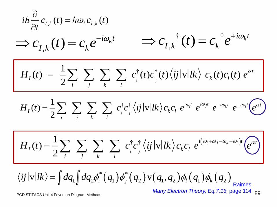
89 PCD STiTACS Unit 4 Feynman Diagram Methods
, ,( ) ( )I k k I ki c t c tt
, ( ) ki t
I k kc t c e
† †
, ( ) ki t
I k kc t c e
† †1 ( ) ( ) ( ) v ( ) ( )
2 i j
t
I k l
i j k l
H t c t c t ij lk c t c t e
† †1( ) v
2
ji k l
i j
i ti t i t i t t
I k l
i j k l
H t c c ij lk c c e e e e e
† †1( ) v
2
i j k l
i j
i t t
I k l
i j k l
H t c c ij lk c c e e
Raimes
Many Electron Theory, Eq.7.16, page 114
* *
1 2 1 2 1 2 1 2v v ,i j l kij lk dq dq q q q q q q

90 PCD STiTACS Unit 4 Feynman Diagram Methods
1
10 0
limt
E i At
1 0 1 0
0 1 1 0
( ) t
I
A U
idt H t
† †1( ) v
2
i j l k
i j
i t t
I k l
i j k l
H t c c ij lk c c e e
α switch
1
1
1 0 1 0
† †
, , ,0 1 0
1v
2 i j
i j l k
t k lt
i j k l
i t
A U
c c ij lk c cidt e
e
↓ Note: ↓ integration variable is t1

91 PCD STiTACS Unit 4 Feynman Diagram Methods
1
1 0 1 0
† †
, , ,0 1 0
1v
2
i j
i j l k
t k lt
i j k l
i t
A U
c c ij lk c cidt e
e
1 1 11 1 1
1 1 1
1
i j l kt t ti t i ti t tt
i j l k
I dt e e dt e e dt e
where
1 1 1 1
1 1
1
1 1
ti t t i t t
t i t e e e eI dt e
i i
1
† †
1 0 1 0 0 0
, , , 1
v 2 i j
i t
k l
i j k l
i eA U c c ij lk c c
i

92 PCD STiTACS Unit 4 Feynman Diagram Methods
2 3
1 1 1
4 5
1 1
0
0
1 1
2 3
1 1 ....
4 5
limn n n
n n n
n n
n n t
A A A
E it
A A
1
10 0
limt
E
i At
1
† †
1 0 1 0 0 0
, , , 1
v 2 i j
i t
k l
i j k l
i eA U c c ij lk c c
i
1† †1
0 0 1
, , , 1
1 v
2 i j
i t
k l
i j k l
A ic c ij lk c c i e
t i
1† †10 0 0 0
, , ,
v ( )2 i j
i t
k l I
i j k l
A i ic c ij lk c c e H t
t
† †1( ) v
2
i j l k
i j
i t t
I k l
i j k l
H t c c ij lk c c e e

93 PCD STiTACS Unit 4 Feynman Diagram Methods
1
1 † †
0 0
, , , 10
0
v 2
limi j
i t
k l
i j k lt
i eE i c c ij lk c c
t i
1
0 0
† †
0 0
, , ,
'
1= v
2 i j k l
i j k l
E H
c c c c ij lk
α0 not relevant for
first order correction;
but not so for higher
order terms…..
1† †10 0 0 0
, , ,
v ( )2 i j
i t
k l I
i j k l
A i ic c ij lk c c e H t
t
† †1( ) v
2
i j l k
i j
i t t
I k l
i j k l
H t c c ij lk c c e e
with
10 0 0 0
0
0 'I
t
A i iH t H
t
Eq.6.35/Raimes
Page 108

94 PCD STiTACS Unit 4 Feynman Diagram Methods
1 † †
0 0
, , ,
1 v
2 i j k l
i j k l
E c c c c ij lk
Now, before we consider higher order terms,
recapitulate that:
1 0 1 0
0 1 1 0
( ) t
I
A U
idt H t
10 1 1 0
0 0
( )
( )
t
I
I
A idt H t
t t
iH t
Resulted in:

95 PCD STiTACS Unit 4 Feynman Diagram Methods
1 † †
0 0
, , ,
1 v
2 i j k l
i j k l
E c c c c ij lk
0 0
0 1 2 1 2 0
1 .. ( ) ( ).. ( )
!
n n
nt t t
n I I I n
A U
idt dt dt T H t H t H t
n
1 2 3 ..E E E E
indexed th
In order corrections by the power of H
2 3
1 1 1
4 5
1 1 0
0
1 1
2 3
1 1 ....
4 5
limn n n
n n n
n n
n nt
A A A
E it
A A
Now, we shall consider higher order terms:

96 PCD STiTACS Unit 4 Feynman Diagram Methods
0 0
0 1 2 1 2 0
1 .. ( ) ( ).. ( )
!
n n
nt t t
n I I I n
A U
idt dt dt T H t H t H t
n
2 3
1 1 1
4 5
1 1
0
0
1 1
2 3
1 1 ....
4 5
limn n n
n n n
n n
n n t
A A A
E it
A A
22
2 10 0
1
2lim
tE i A A
t
22
2 10 00 0
2
lim limt t
iE i A A
t t

97 PCD STiTACS Unit 4 Feynman Diagram Methods
T: Time-ordered product of operators. Operators containing the latest time stand farthest to the left.
2
'
, =1 ' ( ') ' '' ( ') ( '') .. t t t
I I I
i iU t dt H t dt dt H t H t
1 21 2
0
( ) ( ).. ( )1
, = .. !
nt t t
I n
n
I InTi
U t dt dt d H t H t tt Hn
Equivalent form:
1
1 2 1 22
1 ( ) ( )
t t
I Idt dt H t H t
2nd order term
: we shall use
, : switcht
Note
U t e
1 1 tH e H

98 PCD STiTACS Unit 4
Feynman Diagram
Methods
22
2 10 00 0
2
lim limt t
iE i A A
t t
2 0 2 0 2 0 2 0; hence A U A Ut t
1
2 0 1 1 2 2 02
1 ( ) ( )
t t
I IA dt H t dt H tt t
1
2 0 1 1 2 2 02
1 ( ) ( )
t t
I IA dt H t dt H tt t
0 1 1 0 0 0from Slide 94: ( ) ( )t
I I
i idt H t H t
t
2 0 2 2 02
1 ( ) ( )
t
I IA H t dt H tt

99
0 1 0 t
tH H e H H
0 0
1 ( )
( ) 0
H Hi t i t
t
I
I
H t e e H e
H t
2 0 2 2 02
1 ( ) ( )
t
I IA H t dt H tt
0
2 0 2 2 020
1 ( 0) ( ) I I
t
A H t dt H tt
0
2 0 020
1 ( 0) ( ) I I
t
A H t dt H tt
Using t instead of t2 ↑
PCD STiTACS Unit 4 Feynman Diagram Methods

100 PCD STiTACS Unit 4 Feynman Diagram Methods
0
2 0 020
1 ( 0) ( ) I I
t
A H t dt H tt
0 0
1 1 ( ) i.e. ( 0)H H
i t i tt
I IH t e e H e H t H
0
2 0 1 020
1 ( ) I
t
A H dt H tt
0 00
2 0 1 1 020
1
H Hi t i t
t
t
A dt H e e H et
0 00
2 0 1 1 020
1
H Ei t i t
t
t
A dt H e H e et
Raimes
Many Electron Theory, Eq.6.39, page 109

101 PCD STiTACS Unit 4 Feynman Diagram Methods
0 00
2 0 1 1 020
1
H Ei t i t
t
t
A dt H e H e et
0 0
*
0 1 1 0 0 1 1 0 ' H H
i t i t
H e H dV H e H
space integral
0 0
*
0 1 1 0 1 0 1 0 ' H H
i t i t
H e H dV H e H
1 0
0
1 0 1 0
0 0
m m
m
m m m m
m m
H c
H H

102 PCD STiTACS Unit 4 Feynman Diagram Methods
0 0
*
0 1 1 0 1 0 1 0 ' H H
i t i t
H e H dV H e H
1 0 1 0
0
m m
m
H H
0
0
0 1 1 0
*
0 1 1 0
0 0
'
Hi t
Hi t
n n m m
n m
H e H
dV H e H
0
*
0 1 1 0
0 0
' H
i t
n m n m
n m
H H dV e

PCD STiTACS Unit 4 Feynman Diagram Methods 103
*
0 1 1 0
0 0
' mE
i t
n m n m
n m
H H e dV
0
*
0 1 1 0
0 0
' H
i t
n m n m
n m
H H dV e
0
0 1 1 0 H
i t
H e H
nm
0
0 1 1 0 0 1 1 0
0 0
mH E
i t i t
n m nm
n m
H e H H H e

104 PCD STiTACS Unit 4 Feynman Diagram Methods
0
0 1 1 0 0 1 1 0
0
nH E
i t i t
n n
n
H e H H H e
0 2
0 1 1 0 1 0
0
nH E
i t i t
n
n
H e H H e
0 00
2 0 1 1 020
1
H Ei t i t
t
t
A dt H e H e et
020
2 1 020 0
1
nE Ei t i t
t
n
t n
A dt H e e et

105 PCD STiTACS Unit 4 Feynman Diagram Methods
020
2 1 020 0
1
nE Ei t i t
t
n
t n
A dt H e e et
02 0
2 1 020 0
1
nE E ii t
n
t n
A H dt et
02 0
2 1 020 0
1
nE E ii t
n
t n
A H dt et
0
0
0
0
0 0
n
n
E Ei tE E i t
i t
n n
e edt e
E E i i E E ii

106 PCD STiTACS Unit 4 Feynman Diagram Methods
02 0
2 1 020 0
1
nE E ii t
n
t n
A H dt et
0
0
0
0
0 0
n
n
E Ei tE E i t
i t
n n
e edt e
E E i i E E ii
2
1 0
2
0 0 0
1
n
t n n
HA
t i E E i
22
2 10 00 0
2
lim limt t
iE i A A
t t
?
Questions: [email protected]

Select/Special Topics from ‘Theory of Atomic Collisions and Spectroscopy’
107
P. C. Deshmukh
Department of Physics
Indian Institute of Technology Madras
Chennai 600036
Feynman Diagrams
PCD STiTACS Unit 4 Feynman Diagram Methods
Unit 4 Lecture Number 29
Feynman Diagram Methods

108 PCD STiTACS Unit 4 Feynman Diagram Methods
1 2 3 ..E E E E
2 2 2
1 2 3
1 2 3 1 2 1 3 1 4
2 1 2 3 2 4
3 3 3
1 2 3 1 2 3
2 2 2
1 2 1 3 1 4 2 1 3
2 2 2
2 1 2 3 2 4
0
...1
...2
..
... ...1
... ...3
....
lim
A A A
A A A A A A A A A
A A A A A AE i
t A A A A A A
A A A A A A A A A
A A A A A A
0
....
...t
0 0
0 1 2 1 2 0
1 .. ( ) ( ).. ( )
!
n n
nt t t
n I I I n
A U
idt dt dt T H t H t H t
n
Chronological operator

109 PCD STiTACS Unit 4 Feynman Diagram Methods
1
1 † †
0 0
, , , 10
0
v 2
limi j
i t
k l
i j k lt
i eE i c c ij lk c c
t i
1
0 0
† †
0 0
, , ,
'
1= v
2 i j k l
i j k l
E H
c c c c ij lk
α0 not relevant for
first order correction;
but not so for higher
order terms…..
1 0 1 0 0 1 1 0 ( ) t
I
iA U dt H t
1 1 1 1
1 1
1
1 1
ti t t i t t
t i t e e e eI dt e
i i
10 1 1 0 0 0 ( ) ( )
t
I I
A i idt H t H t
t t
1
10 0
limt
E i At

110 PCD STiTACS Unit 4 Feynman Diagram Methods
0 0
0 1 2 1 2 0
1 .. ( ) ( ).. ( )
!
n n
nt t t
n I I I n
A U
idt dt dt T H t H t H t
n
2 3
1 1 1
4 5
1 1
0
0
1 1
2 3
1 1 ....
4 5
limn n n
n n n
n n
n n t
A A A
E it
A A
22
2 10 0
1
2lim
tE i A A
t
22
2 10 00 0
2
lim limt t
iE i A A
t t

111 PCD STiTACS Unit 4
Feynman Diagram
Methods
22
2 10 00 0
2
lim limt t
iE i A A
t t
2 0 2 0 2 0 2 0; hence A U A Ut t
1
2 0 1 1 2 2 02
1 ( ) ( )
t t
I IA dt H t dt H tt t
2 0 2 2 02
1 ( ) ( )
t
I IA H t dt H tt
at t=0

112 PCD STiTACS Unit 4 Feynman Diagram Methods
0 00
2 0 1 1 020
1
H Ei t i t
t
t
A dt H e H e et
0 0
*
0 1 1 0 1 0 1 0 ' H H
i t i t
H e H dV H e H
1 0 1 0 1 0
0 0 0
m m m m m m
m m m
H c H H
020
2 1 020 0
1
nE Ei t i t
t
n
t n
A dt H e e et

113 PCD STiTACS Unit 4 Feynman Diagram Methods
02 0
2 1 020 0
1
nE E ii t
n
t n
A H dt et
0
0
0
0
0 0
n
n
E Ei tE E i t
i t
n n
e edt e
E E i i E E ii
2
1 0
2
0 0 0
1
n
t n n
HA
t i E E i
22
2 10 00 0
2
lim limt t
iE i A A
t t
?

114 PCD STiTACS Unit 4 Feynman Diagram Methods
1 0 1 1 0 ( ) t
I
iA dt H t
10 0 ( ) I
A iH t
t
2
1 0 1 1 0 0 02
2 ( ) ( )
t
I IA dt H t H tt
02
1 0 1 1 0 0 020
2 ( ) ( 0)I I
t
A dt H t H tt
2 1
1 12A
A At t
2
10 0
?2
limt
iA
t
?
( 0)t
115 PCD STiTACS Unit 4 Feynman Diagram Methods
0 0
1 1 ( ) ( ) 0 ( 0)H H
i t i tt
I I IH t e e H e H t H t H
02
1 0 1 1 0 0 020
2 ( ) ( 0)I I
t
A dt H t H tt
02
1 0 0 0 1 020
2 ( ) I
t
A dt H t Ht
0 00 0
0 0 010( ) H H
i t i tt
Idt dt tH e e H e
0 00 0
0 0 0 1 0 ( ) E E
i t i tt
Idt H t dt e e H e

116
PCD STiTACS Unit 4 Feynman Diagram
Methods
02
1 0 0 0 1 020
2 ( ) I
t
A dt H t Ht
0 00 0
0 0 0 1 0 ( ) E E
i t i tt
Idt H t dt e e H e
0
0 1 0 tdt e H
0
0 1 0 te
H
0 1 0 H
2 0 1 0
1 0 1 020
2
t
HA H
t

117 PCD STiTACS Unit 4 Feynman Diagram Methods
22
2 10 00 0
2
lim limt t
iE i A A
t t
2 0 1 0
1 0 1 020
2
t
HA H
t
2
1 0
2
0 0 0
1
n
t n n
HA
t i E E i
2
1 0 0 1 02
0 1 020 0
0
1 2
2lim
n
n n
H HiE i H
i E E i
2 2
1 0 0 1 02
0 00
+ lim
n
n n
H HiE
E E i
118 PCD STiTACS Unit 4 Feynman Diagram Methods
2 2
1 0 0 1 02
0 00
+ lim
n
n n
H HiE
E E i
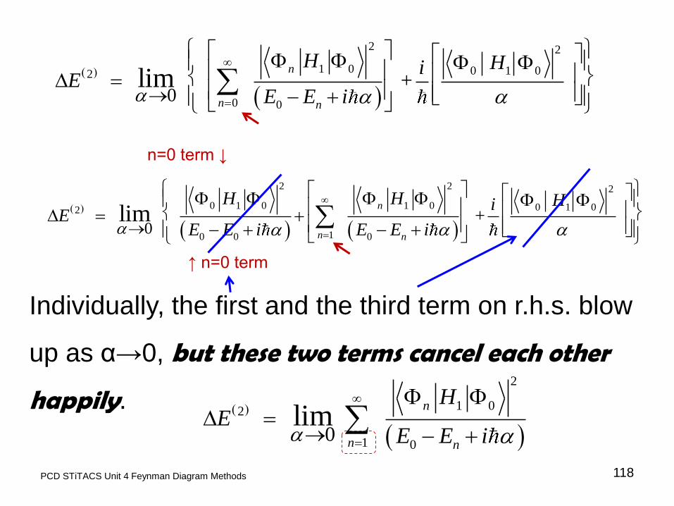
Individually, the first and the third term on r.h.s. blow
up as α→0, but these two terms cancel each other
happily.
2 2 2
0 1 0 1 0 0 1 02
10 0 00
+ lim
n
n n
H H HiE
E E i E E i
↑ n=0 term
2
1 02
1 00
limn
n n
HE
E E i
n=0 term ↓

119 PCD STiTACS Unit 4 Feynman Diagram Methods
2
1 0
1 0
n
n n
H
E E
α→0 was needed to see correspondence with
Rayleigh-Schrodinger perturbation theory.
Raimes Many Electron Theory, Eq.6.48, page 111
2
1 02
1 00
limn
n n
HE
E E i
Same result holds good for higher order terms.
Same as 2nd order
Rayleigh-Schrodinger
perturbation theory.

120 PCD STiTACS Unit 4 Feynman Diagram Methods
If it is the same result as Rayleigh-Schrodinger
Perturbation Theory, what is the advantage?
Combined with time-dependent methods and
FEYNMAN DIAGRAMS, the present method
offers tremendous convenience, specially in
addressing higher order corrections.
2
1 02
1 0
n
n n
HE
E E
PCD STiTACS Unit 4 Feynman
Diagram Methods
121
The technique of adiabatic switching,
and
addressing the perturbations
using the methods we discussed
can be applied to many other situations;
not just a many-electron system.

PCD STiTACS Unit 4 Feynman Diagram Methods 122
1
2 0 1 1 2 2 02
1 ( ) ( )
t t
I IA dt H t dt H t
We have seen the second order term:
Let us get an advance glance at the nth
order term:

1 2
, , , , , , , , ,
2 2
....
1 2
....2
v
v
....
v
1
.... 1
1....
....
n
n
i j k l p q r s u w x y
n
n
i n t
n
i
ij lk
pq sr
uw yx
i n
i
e
i n
† † † † † †0 0
....i j pk l q r s u w x yc c c c c c c c c c c c
123 PCD STiTACS Unit 4 Feynman Diagram Methods
complex? 0 0 n nA U

Mediator
(Boson)
PHOTON
124 PCD STiTACS Unit 4 Feynman Diagram Methods
“I learned very early the difference between
knowing the name of something, and
knowing something.” ― Richard P. Feynman (1918-1988)
http://www.goodreads.com/author/quotes/1429989.Richard_P_Feynman
Downloaded on December 09, 2013 particle creation
particle destruction
Vertex is where an interaction between
interacting particles is indicated
hole creation
hole destruction

125 PCD STiTACS Unit 4 Feynman Diagram Methods
Our interest in the present course:
Select/Special Topics
in the
Theory of Atomic Collisions and Spectroscopy
Study of electron-correlation effects in atomic
collision / photoabsorption processes -
-Random Phase Approximation
-Many Body Perturbation Theory
-Configuration Interactions …… etc.
-RRPA: Relativistic Random Phase Approximation
-MCTD: MultiConfiguration Tamm Dancoff method
-MQDT: Multichannel Quantum Defect Theory etc…
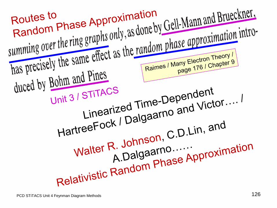
126 PCD STiTACS Unit 4 Feynman Diagram Methods

127 PCD STiTACS Unit 4 Feynman Diagram Methods
† †
1
1 v
2 i j k l
i j k l
H c c ij lk c c
0 1
tH H e H
We shall use the INTERACTION PICTURE
formalism.
0 0
0
, ,
H Hi t i t
I S
Hi t
I S
e e
r t e r t
0 0
1 ( ) H H
i t i tt
IH t e e H e
0 0
1( ) H H
i t i t
IH t e H e
Adiabatic switching on
of the interaction.

128 PCD STiTACS Unit 4 Feynman Diagram Methods
0 0
1 ( )
( ) 0
H Hi t i t
t
I
I
H t e e H e
H t
† †1 ( ) ( ) ( ) v ( ) ( )
2 i j
t
I k l
i j k l
H t c t c t ij lk c t c t e
0 1 tH H e H
α: adiabatic switch
control parameter
0 00 0
log ,limt
E i U tt
From U4L26/Slide 66:
Correction to the energy due to the interaction between
the many-particle electron system.

129 PCD STiTACS Unit 4 Feynman Diagram Methods
0 00 0
log ,limt
E i U tt
2 3
0 0
1 1 1
4 5
1 1
1 1log ,
2 3
1 1 ....
4 5
n n n
n n n
n n
n n
U t A A A
A A
2 3
1 1 1
4 5
1 1
0
0
1 1
2 3
1 1 ....
4 5
limn n n
n n n
n n
n n t
A A A
E it
A A
0 0
0 1 2 1 2 0
1 .. ( ) ( ).. ( )
!
n n
nt t t
n I I I n
A U
idt dt dt T H t H t H t
n
From U4L26
STiTACS

130 PCD STiTACS Unit 4 Feynman Diagram Methods
1
† †
1 0 1 0 0 0
, , , 1
v 2 i j
i t
k l
i j k l
i eA U ij lk c c c c
i
Slide 80 / U4L27 ; Raimes / Many Electron
Theory / Eq. 7.18, page 114
2
'
, =1 ' ( ') ' '' ( ') ( '') .... t t t
I I I
i iU t dt H t dt dt H t H t
1 21 2
0
( ) ( ).. ( )1
, = .. !
nt t t
I n
n
I InTi
U t dt dt d H t H t tt Hn
Two equivalent forms of the
Time Evolution Operator:
0 0
1 , since ( ) H H
i t i tt
IWe must use U t H t e e H e
1 i j l k
We shall now consider the 2nd order term; use (A)
(A)
(B)

131 PCD STiTACS Unit 4 Feynman Diagram Methods
2
'
, =1 ' ( ') ' '' ( ') ( '') .. t t t
I I I
i iU t dt H t dt dt H t H t
1
2
2, 1 2 1 2, = ( ) ( )t t
I I
iU t dt dt H t H t
1
2 0 2 0
2
0 1 2 1 2 0
( ) ( ) t t
I I
A U
idt dt H t H t
† †1 ( ) ( ) ( ) v ( ) ( )
2 i j
t
I k l
i j k l
H t c t c t ij lk c t c t e
1 t
e 2
te
* *
1 2 1 2 1 2 1 2v v ,i j l kij lk dq dq q q q q q q
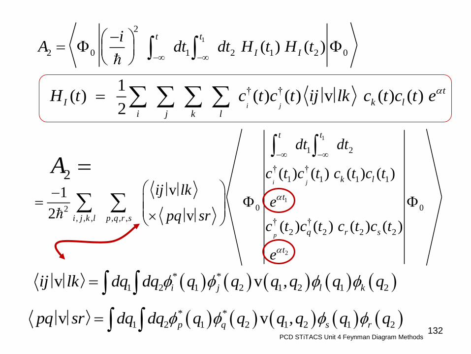
132 PCD STiTACS Unit 4 Feynman Diagram Methods
1
2
2 0 1 2 1 2 0 ( ) ( ) t t
I I
iA dt dt H t H t
† †1 ( ) ( ) ( ) v ( ) ( )
2 i j
t
I k l
i j k l
H t c t c t ij lk c t c t e
* *
1 2 1 2 1 2 1 2v v ,i j l kij lk dq dq q q q q q q
1
1
2
1 2
† †
1 1 1 1
0 02, , , , , , † †
2 2 2 2
( ) ( ) ( ) ( )v1
2 v
( ) ( ) ( ) ( )
i j
p
t t
k l
t
i j k l p q r s
q r s
t
dt dt
c t c t c t c tij lk
epq sr
c t c t c t c t
e
2 A
* *
1 2 1 2 1 2 1 2v v ,p q s rpq sr dq dq q q q q q q

133 PCD STiTACS Unit 4 Feynman Diagram Methods
1
1
2
1 2
† †
1 1 1 1
0 02, , , , , , † †
2 2 2 2
( ) ( ) ( ) ( )v1
2 v
( ) ( ) ( ) ( )
i j
p
t t
k l
t
i j k l p q r s
q r s
t
dt dt
c t c t c t c tij lk
epq sr
c t c t c t c t
e
2 A
, ( ) ki t
I k kc t c e
† †
, ( ) ki t
I k kc t c e
11 1 1 2 2 2
1 2
2, , , , , ,
† † † †0 0
v1
2 v
i j p
t ti t t i t t
i j k l p q r s
k l q r s
dt e e dt e eij lk
pq src c c c c c c c
2 A
1 i j l k 2 p q r s

134 PCD STiTACS Unit 4 Feynman Diagram Methods
11 1 1 2 2 2
1 2
2, , , , , ,
† † † †0 0
v1
2 v
i j p
t ti t t i t t
i j k l p q r s
k l q r s
dt e e dt e eij lk
pq src c c c c c c c
2 A
1 i j l k 2 p q r s
11 1 1 2 2 2
1 2 ?t t
i t t i t tdt e e dt e e
12 2 2
2 ?t
i t tdt e e
12 2 2 1
1 12 22 2 2
2 2
2 2
ti t i t
t t i ti t t e edt e e dt e
i i

135 PCD STiTACS Unit 4 Feynman Diagram Methods
11 1 1 2 2 2
1 2 ?t t
i t t i t tdt e e dt e e
2 11
2 2 2
2
2
i t
ti t t e
dt e ei
2 1
2 11 1 1 1 1 1
1 1
2 2
1i t
t t i ti t t i t tedt e e dt e e e
i i
1 21
1 1 1 2 2 2
2
1 2
2 1 2
1
2
i tt t
i t t i t t edt e e dt e e
i i
1 2 12
1
2
1 t i tdt e
i
1 2 12 1
1 1 1
2
1
2 2 1 2
1
2
ti ti t
ti t t e e
dt e ei i i

136 PCD STiTACS Unit 4 Feynman Diagram Methods
11 1 1 2 2 2
1 2
2, , , , , ,
† † † †0 0
v1
2 v
i j p
t ti t t i t t
i j k l p q r s
k l q r s
dt e e dt e eij lk
pq src c c c c c c c
2 A
1 i j l k 2 p q r s
1 21
1 1 1 2 2 2
2
1 2
2 1 2
1
2
i tt t
i t t i t t edt e e dt e e
i i
1 2
2
† † † †0 02 2, , , , , ,
1 2
1
v1
2 v
2
i j p
i ti j k l p q r s k l q r s
iij lk
c c c c c c c cepq sr
i
2 A
Raimes / Many Electron Theory / Eq. 7.20, page 115 Next: generalize the
pattern for nth term…..

137 PCD STiTACS Unit 4 Feynman Diagram Methods
1 2
2
† † † †0 02 2, , , , , ,
1 2
1
v1
2 v
2
i j p
i ti j k l p q r s k l q r s
iij lk
c c c c c c c cepq sr
i
2 A
nth order term….
One may generalize the pattern we have
seen above….
2 3
1 1 1
4 5
1 1
0
0
1 1
2 3
1 1 ....
4 5
limn n n
n n n
n n
n n t
A A A
E it
A A
0 0
0 1 2 1 2 0
1 .. ( ) ( ).. ( )
!
n n
nt t t
n I I I n
A U
idt dt dt T H t H t H t
n

1 2
, , , , , , , , ,
2 2
....
1 2
....2
v
v
....
v
1
.... 1
1....
....
n
n
i j k l p q r s u w x y
n
n
i n t
n
i
ij lk
pq sr
uw yx
i n
i
e
i n
† † † † † †0 0
....i j pk l q r s u w x yc c c c c c c c c c c c
138 PCD STiTACS Unit 4 Feynman Diagram Methods
complex? 0 0 n nA U
Questions:
Select/Special Topics from ‘Theory of Atomic Collisions and Spectroscopy’
139
P. C. Deshmukh
Department of Physics
Indian Institute of Technology Madras
Chennai 600036
PCD STiTACS Unit 4 Feynman Diagram Methods
I Order Feynman Diagrams
Unit 4 Lecture Number 30
Feynman Diagram Methods
140 PCD STiTACS Unit 4 Feynman Diagram Methods
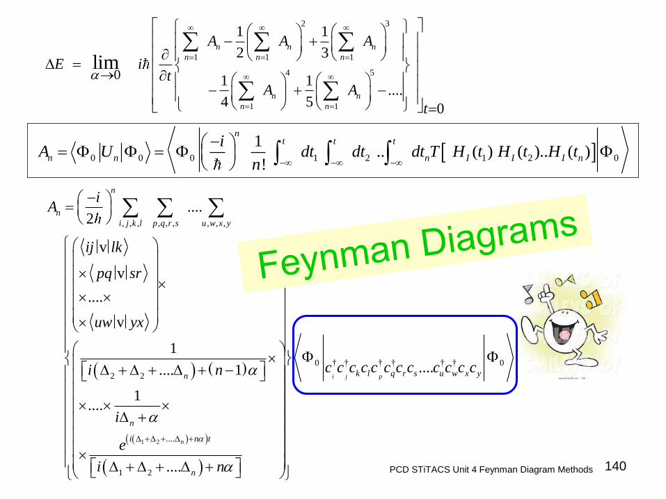
2 3
1 1 1
4 5
1 1
0
0
1 1
2 3
1 1 ....
4 5
limn n n
n n n
n n
n n t
A A A
E it
A A
0 0 0 1 2 1 2 0
1 .. ( ) ( ).. ( )
!
n
t t t
n n n I I I n
iA U dt dt dt T H t H t H t
n
1 2
, , , , , , , , ,
2 2
....
1 2
....2
v
v
....
v
1
.... 1
1....
....
n
n
n
i j k l p q r s u w x y
n
n
i n t
n
iA
ij lk
pq sr
uw yx
i n
i
e
i n
† † † † † †0 0
....
i j pk l q r s u w x yc c c c c c c c c c c c

141 PCD STiTACS Unit 4 Feynman Diagram Methods
Transformation of particles (electrons)
to particles
and holes 1
0 : single Slater determinant
of elements ( )k
q
The present technique can be easily extended for more
complex systems, such as electron gas in a periodic lattice
potential.
For FREE ELECTRONS: Fermi surface is a sphere

142 PCD STiTACS Unit 4 Feynman Diagram Methods
Transformation of particles (electrons) to excited particle
states above Fermi surface, and vacant hole states below it.
For FREE ELECTRONS: Fermi surface is a sphere.
occupied; vacantF Fk k k k
↑ Occupied and unoccupied states are described
simply, but it can still be easily done in other cases.
vectors: lie inside Fermi sphere of radius Fk k
10 : single Slater determinant of elements ( )
kq

143 PCD STfTACS Unit 2 Many-body theory, electron correlations, Feynman-Goldstone diagrams
12 Z
2 2 2 4 2
1 1 1 1 3 1
2 2 2 2 2
1 2 2 2 3SD s s p p s
2 2 2 4 2
2 1 1 1 3 1
2 2 2 2 2
1 2 2 2 3SD s s p p p
Slater
determinant
….. Many different Slater determinants
can be used!
Multi-configuration Hartree-Fock:
CI: Configuration Interaction

PCD STiTACS Unit 4 Feynman Diagram Methods 144
Bubbles
in boiling
water
Creation
and
Annihilation
of particles
and holes
…
above/below
EF

1 2
, , , , , , , , ,
2 2
....
1 2
....2
v
v
....
v
1
.... 1
1....
....
n
n
i j k l p q r s u w x y
n
n
i n t
n
i
ij lk
pq sr
uw yx
i n
i
e
i n
† † † † † †0 0
....i j pk l q r s u w x yc c c c c c c c c c c c
145 PCD STiTACS Unit 4 Feynman Diagram Methods
2 3
1 1 1
4 5
1 1
0
0
1 1
2 3
1 1 ....
4 5
limn n n
n n n
n n
n n t
A A A
E it
A A
2
'
, =1 ' ( ') ' '' ( ') ( '') .... t t t
I I I
i iU t dt H t dt dt H t H t
nA

146 PCD STiTACS Unit 4 Feynman Diagram Methods
occupied and vacantF Fk k k k
states within the Fermi sphere: UNEXCITED
If an unexcited (i.e. below the Fermi level) state is unoccupied by an electron,
then it is called a “hole” state.
Destruction of an electron in an unexcited (i.e. below
the Fermi level) ↔ creation of a hole.
Creation of an electron in an unoccupied unexcited
(i.e. below the Fermi level) ↔ destruction of a hole.
states above (“outside; in the momentum-space”)
the Fermi sphere: EXCITED
How would you create a hole state?
How would you now destroy that hole state?

PCD STiTACS Unit 4 Feynman Diagram Methods
occupied and vacantF Fk k k k
, ( ) ki t
I k kc t c e
† †
, ( ) ki t
I k kc t c e
Electron
destruction
and
creation
operators
k ka c† †
k ka c†
k kb c
†
k kb c
hole
destruction
and
creation
operators
Electron
operators
act at all ε
particle
operators
act at ε > εF
hole
operators
act at ε ≤ εF
, ( ) ki t
I k ka t a e
† †
, ( ) ki t
I k ka t a e
, ( ) ki t
I k kb t b e
† †
, ( ) ki t
I k kb t b e
147
particle and hole
operators in the
interaction picture
particle
destruction
and
creation
operators

148 PCD STiTACS Unit 4 Feynman Diagram Methods
occupied and vacantF Fk k k k
k ka c† †
k ka c
particle
destruction
and
creation
operators
†
k kb c
†
k kb c
hole
destruction
and
creation
operators
particle
operators
act at ε > εF
hole
operators
act at ε ≤ εF
, ( ) ki t
I k kb t b e
† †
, ( ) ki t
I k kb t b e
†
k k
F
c b
if k k
† †
k k
F
c a
if k k
k k
F
c a
if k k
†
k k
F
c b
if k k

149 PCD STiTACS Unit 4 Feynman Diagram Methods
Feynman diagrams/graphs
(2005)
QED: electrons exchange virtual photons which mediate
the interaction between the electrons.
The electromagnetic interaction is treated at the level of
quantum theory.
positron: electron propagating backward in time
particle lines
point upwards hole lines point
downwards
AMO Physics: no positrons; but there are ‘hole’ states…
……vacant states normally occupied by electrons
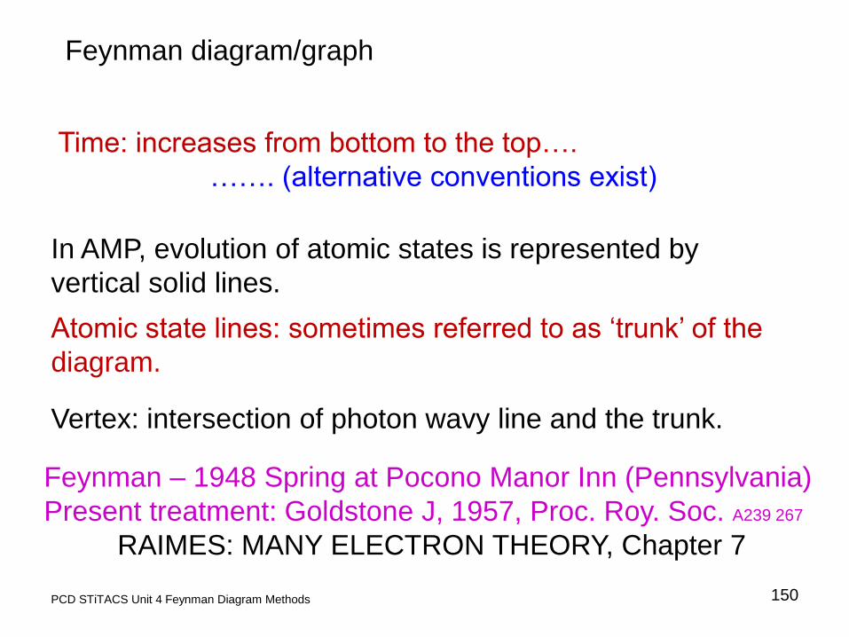
150 PCD STiTACS Unit 4 Feynman Diagram Methods
Feynman diagram/graph
Time: increases from bottom to the top….
……. (alternative conventions exist)
Vertex: intersection of photon wavy line and the trunk.
In AMP, evolution of atomic states is represented by
vertical solid lines.
Atomic state lines: sometimes referred to as ‘trunk’ of the
diagram.
Feynman – 1948 Spring at Pocono Manor Inn (Pennsylvania)
Present treatment: Goldstone J, 1957, Proc. Roy. Soc. A239 267
RAIMES: MANY ELECTRON THEORY, Chapter 7

151 PCD STiTACS Unit 4 Feynman Diagram Methods
particle lines
point upwards
hole lines point
downwards
Wiggly lines: mediators of the interaction
photons
Vertex: indicates where the interaction occurs
particle and hole lines go in or out
of a vertex……
….depending on particle/hole
creation/destruction……
Principal elements of a Feynman diagram/graph
It does not matter whether these lines lean
toward left or right; or do not lean at all….

Line pointing
down, out of the
vertex:
destruction of a
hole in an
unexcited state
ε<εF
Line pointing up, out
of the vertex:
creation of a particle
in an excited state
ε>εF
Mediator
(Boson)
PHOTON
152 PCD STiTACS Unit 4 Feynman Diagram Methods
particle creation
particle destruction Vertex is where an interaction is indicated
hole creation
hole destruction
†; i i Fa
Line pointing up,
Into the vertex:
destruction of a particle
in an excited state ε>εF
; i i Fa
†; j j Fb
; j j Fb
Line pointing
down, into the
vertex:
creation of a hole
in an unexcited
state ε<εF

1 2
, , , , , , , , ,
2 2
....
1 2
....2
v
v
....
v
1
.... 1
1....
....
n
n
i j k l p q r s u w x y
n
n
i n t
n
i
ij lk
pq sr
uw yx
i n
i
e
i n
† † † † † †0 0
....i j pk l q r s u w x yc c c c c c c c c c c c
153 PCD STiTACS Unit 4 Feynman Diagram Methods
2 3
1 1 1
4 5
1 1
0
0
1 1
2 3
1 1 ....
4 5
limn n n
n n n
n n
n n t
A A A
E it
A A
2
'
, =1 ' ( ') ' '' ( ') ( '') .... t t t
I I I
i iU t dt H t dt dt H t H t
nA

154 PCD STiTACS Unit 4 Feynman Diagram Methods
1
1 0 1 0
† †
0 0
, , , 1
v 2 i j
i t
k l
i j k l
A U
i eij lk c c c c
i
† †
0 0v i j k lij lk c c c c
FIRST ORDER FEYNMAN DIAGRAMS
1 i j l k
, , ,
for some particular
i j k l
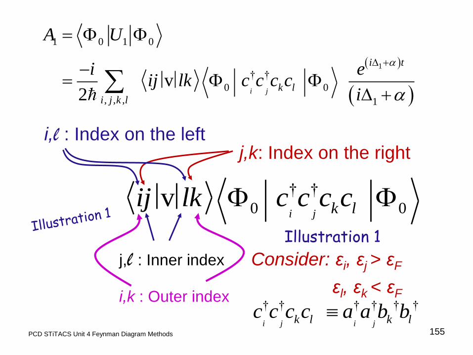
155 PCD STiTACS Unit 4 Feynman Diagram Methods
1
1 0 1 0
† †
0 0
, , , 1
v 2 i j
i t
k l
i j k l
A U
i eij lk c c c c
i
† †
0 0v i j k lij lk c c c c
j,k: Index on the right i,l : Index on the left
j,l : Inner index
i,k : Outer index
Consider: εi, εj > εF
εl, εk < εF † † † † † † i j i jk l k lc c c c a a b b
Illustration 1

156 PCD STiTACS Unit 4 Feynman Diagram Methods
† †
0 0v i j k lij c c c clk
j,k: Index on the right i,l : Index on the left
j,l : Inner index
i,k : Outer index
Consider: εi, εj > εF
εl, εk < εF † † † † † † i j i jk l k lc c c c a a b b
particle
creation
particle
destruction
hole creation
hole destruction
kl
Right vertex Left vertex
i j
Look at inner/outer indices

157 PCD STiTACS Unit 4 Feynman Diagram Methods
† †
0 0v i j k lij c c c clk
j,k: Index on the right i,l : Index on the left
Consider: εi, εj > εF
εl, εk < εF † † † † † † i j i jk l k lc c c c a a b b
particle
creation
particle
destruction
hole creation
hole destruction
kli j
l
k
i
j

158 PCD STiTACS Unit 4 Feynman Diagram Methods
† †
0 0v i j k lij c c c clk
j,k: Index on the right i,l : Index on the left
Consider: εi, εj < εF
εl, εk > εF † † i j k l i j k lc c c c bb a a
particle
creation
particle
destruction
hole creation
hole destruction
kli j
l
k i
j

j
159 PCD STiTACS Unit 4 Feynman Diagram Methods
† †
0 0v i j k lij c c c clk
j,k: Index on the right i,l : Index on the left
Consider: εi, εj < εF
εl, εk > εF † † i j k l i j k lc c c c bb a a
kli
l
k i
j

li
160 PCD STiTACS Unit 4 Feynman Diagram Methods
† †
0 0v i j k lij c c c clk
j,k: Index on the right i,l : Index on the left
Consider: εi, εj , εk > εF
εl < εF † † † † † i j i j lk l kc c c c a a a b
particle
creation
particle
destruction
hole creation
hole destruction
kRight vertex Left vertex
j
Look at inner/outer indices
Outer Inner Inner Outer
l
i j
k

l
i
161 PCD STiTACS Unit 4 Feynman Diagram Methods
† †
0 0v i j k lij c c c clk
j,k: Index on the right i,l : Index on the left
Consider: εi, εj , > εF
εl, εk > εF † † † † i j i jk l k lc c c c a a a a
particle
creation
particle
destruction
hole creation
hole destruction
k
j
Outer Inner Inner Outer
l
k
i
j

162 PCD STiTACS Unit 4 Feynman Diagram Methods
Consider: εi, εj , > εF
εl, εk > εF
† † † † i j i jk l k lc c c c a a a a
particle
creation
particle
destruction
hole creation
hole destruction
k l
ij
l
i
k
j
left right
Interchange vertices
V V
† † † † j i il k j l kc c c c a a a a
equivalent Fig.7.8/page123
Raimes/MET
If either i=j or k=l, the
term becomes zero

163 PCD STiTACS Unit 4 Feynman Diagram Methods
Consider: εi, εj , > εF
εl, εk > εF
† † † † i j i jk l k lc c c c a a a a
kl
ij
l
i
k
j
Interchange
two lines
i j
† † † † j i ik l j k lc c c c a a a a
Opposite
sign
Fig.7.9/page124
Raimes/MET
If either i=j or k=l, the
term becomes zero
Questions:

Select/Special Topics from ‘Theory of Atomic Collisions and Spectroscopy’
164
P. C. Deshmukh
Department of Physics
Indian Institute of Technology Madras
Chennai 600036
PCD STiTACS Unit 4 Feynman Diagram Methods
Some more I order Feynman Diagrams
II Order RING Diagrams
Unit 4 Lecture Number 31
Feynman Diagram Methods

l
i
165 PCD STiTACS Unit 4 Feynman Diagram Methods
† †
0 0v i j k lij c c c clk
j,k: Index on the right i,l : Index on the left
Consider: εi, εj > εF
εl, εk > εF † † † † i j i jk l k lc c c c a a a a
particle
creation
particle
destruction
hole creation
hole destruction
k
j
Outer Inner Inner Outer
l
k
i
j

166 PCD STiTACS Unit 4 Feynman Diagram Methods
Consider: εi, εj > εF
εl, εk > εF
† † † † i j i jk l k lc c c c a a a a
particle
creation
particle
destruction
hole creation
hole destruction
k l
ij
l
i
k
j
left right
Interchange vertices
V V
equivalent Fig.7.8/page123
Raimes/MET
If either i=j or k=l, the
term becomes zero

167 PCD STiTACS Unit 4 Feynman Diagram Methods
Consider: εi, εj , > εF
εl, εk > εF
† † † † i j i jk l k lc c c c a a a a
kl
ij
l
i
k
j
Interchange
two lines
i j
Opposite
sign
Fig.7.9/page124
Raimes/MET

i
i
168 PCD STiTACS Unit 4 Feynman Diagram Methods
† †
0 0v i j l ij l c c c ci i
j,l: Index on the right SAME! i,i : Index on the left
Consider: εi < εF & εj, εl > εF
† † † † i j jl i i l ic c c c ba a b
particle
creation
particle
destruction
hole creation
hole destruction
l
j
Outer Inner Inner Outer
l
i
j
l
ji
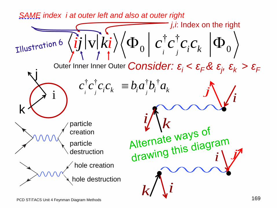
ki
169 PCD STiTACS Unit 4 Feynman Diagram Methods
† †
0 0v i j i kj k c c c ci i
j,i: Index on the right
SAME index i at outer left and also at outer right
Consider: εi < εF & εj, εk > εF
† † † † i j ji k i i kc c c c ba b a
particle
creation
particle
destruction
hole creation
hole destruction
ji
Outer Inner Inner Outer
i
j
k
k i
ji

ki
170 PCD STiTACS Unit 4 Feynman Diagram Methods
† †
0 0v i j i kj k c c c ci i
j,i: Index on the right
SAME index i at outer left and also at outer right
Consider: εi < εF & εj, εk > εF
† † † † i j ji k i i kc c c c ba b a
j i
Outer Inner Inner Outer
k i
ji
j
ki
i
i
k
j
k
j
RAIMES / Fig.7.7 / p.123
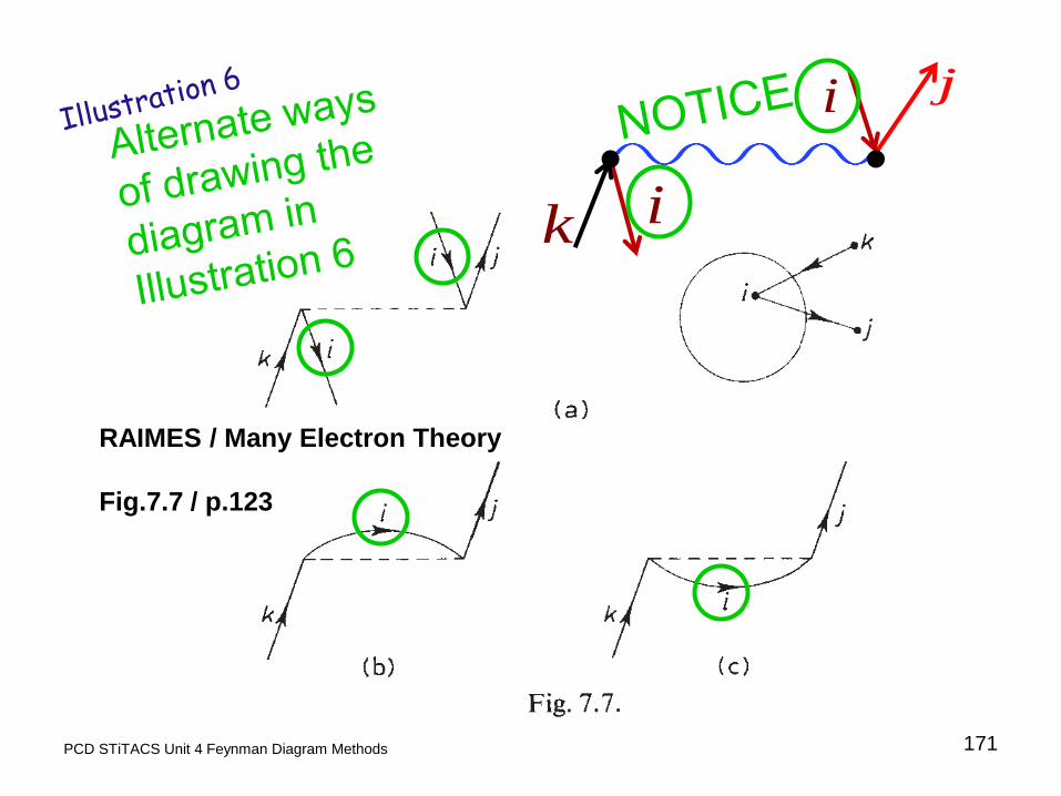
171 PCD STiTACS Unit 4 Feynman Diagram Methods
k
ji
i
RAIMES / Many Electron Theory
Fig.7.7 / p.123
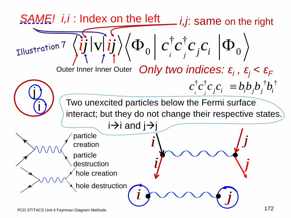
ji
i
i
172 PCD STiTACS Unit 4 Feynman Diagram Methods
† †
0 0v i j j ij j c c c ci i
i,j: same on the right SAME! i,i : Index on the left
Only two indices: εi , εj < εF † † † † i j j i i j j ic c c c bb b b
particle
creation
particle
destruction
hole creation
hole destruction
j
j
Outer Inner Inner Outer
i j
Two unexcited particles below the Fermi surface
interact; but they do not change their respective states.
ii and jj

† †
0 0v i j i jj i c c c ci j
j
i
173 PCD STiTACS Unit 4 Feynman Diagram Methods
j,i: on the right SAME! i,j : Index on the left
Only two indices: εi , εj < εF
† † † † i j i j i j i jc c c c bb b b
hole creation
hole destruction
j
i
Outer Inner Inner Outer
Two unexcited particles below
the Fermi surface interact; and in
this example they exchange their
respective states: ij and ji

† † † †
0 0 0 0
1
,
i j i jj i i j
i j F
ONLY
c c c c and c c c c
with CAN CONTRIBUTE TO A
174 PCD STiTACS Unit 4 Feynman Diagram Methods
1
1 0 1 0
† †
0 0
, , , 1
v 2 i j
i t
k l
i j k l
A U
i eij lk c c c c
i
† †
0 0
† †
0
For - ,
i j
i j
k l
k l
c c c c to be non zero
c c c c must be non zero
0 has neither holes nor excited particles

175 PCD STiTACS Unit 4 Feynman Diagram Methods
† †
0 0v i j j ij j c c c ci i
ji
† †
0 0v i j i jj i c c c ci j
Only two indices:
εi , εj < εF
Opposite
signs
Direct
or
Coulomb
Exchange
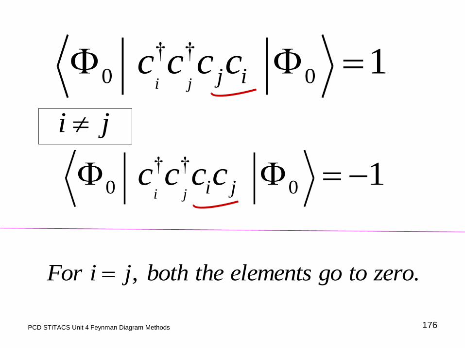
176 PCD STiTACS Unit 4 Feynman Diagram Methods
† †
0 0 1i j j ic c c c
† †
0 0 1i j i jc c c c
, .For i j both the elements go to zero
i j

177 PCD STiTACS Unit 4 Feynman Diagram Methods
1
1 0 1 0 1
† †
0 0
, , , 1
v 2 i j
i j k l
i t
k l
i j k l
A U
i eij lk c c c c
i
Total contribution to A1 from all Direct/Coulomb terms
1
1 0 0
,v 0 & 1
2direct
tA
i j
i j
i eC ij ij
Total contribution to A1 from all Exchange terms
1
1 0 0
,v 0 & 1
2
t
A
exchange
i j
i j
i eC ij ji
, i j F
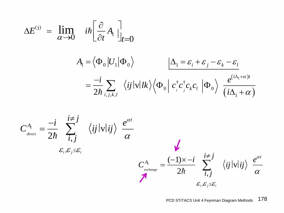
178 PCD STiTACS Unit 4 Feynman Diagram Methods
1
,
,v
2direct
i j i
tA
i j
i j
i eC ij ij
1
,
,
( 1)v
2exchange
i j i
tA
i j
i j
i eC ij ij
1
10 0
limt
E i At
1
1 0 1 0 1
† †
0 0
, , , 1
v 2 i j
i j k l
i t
k l
i j k l
A U
i eij lk c c c c
i

179 PCD STiTACS Unit 4 Feynman Diagram Methods
1
10 0
limt
E i At
1
,
0 , 0
( 1) v + v
2 2lim
i j i
ti j
i j t
i i eE i ij ij ij ji
t
1
,
0 , 0
1 v v
2lim
i j i
t
i j t
eE ij ij ij ji
t
1
,
0 , 0
1 v v
2lim
i j i
t
i j t
eE ij ij ij ji
1
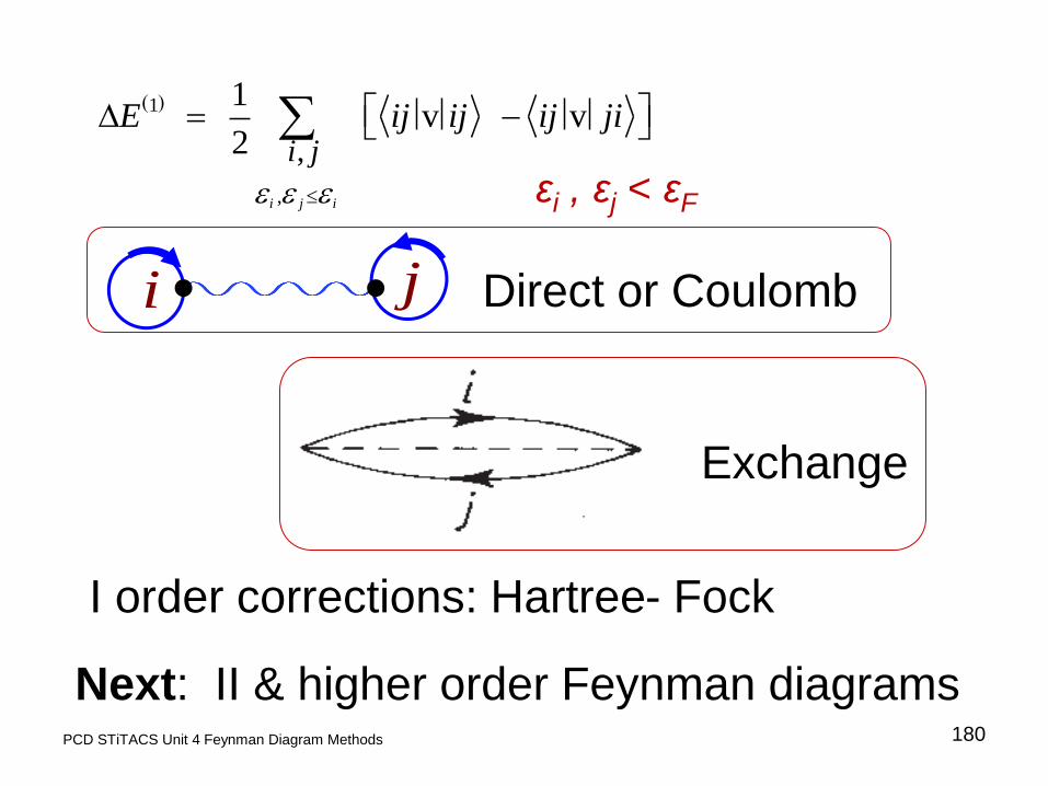
180 PCD STiTACS Unit 4 Feynman Diagram Methods
ji
εi , εj < εF
Direct or Coulomb
Exchange
1
,
,
1 v v
2
i j i
i jE ij ij ij ji
I order corrections: Hartree- Fock
Next: II & higher order Feynman diagrams

181 PCD STiTACS Unit 4 Feynman Diagram Methods
2 3
1 1 1
4 5
1 1
0
0
1 1
2 3
1 1 ....
4 5
limn n n
n n n
n n
n n t
A A A
E it
A A
22
2 10 00 0
2
lim limt t
iE i A A
t t
From: Slide # 95
U4, L28
11 1 1 2 2 2
1 2
2, , , , , ,
† † † †0 0
v1
2 v
i j p
t ti t t i t t
i j k l p q r s
k l q r s
dt e e dt e eij lk
pq src c c c c c c c
2 A From U4L29/S134

182 PCD STiTACS Unit 4 Feynman Diagram Methods
22
2 10 00 0
2
lim limt t
iE i A A
t t
1
1 0 1 0 1
† †
0 0
, , , 1
v 2 i j
i j k l
i t
k l
i j k l
A U
i eij lk c c c c
i
II & higher order Feynman diagrams
1 2
2
† † † †0 02 2, , , , , ,
1 2
1
v1
2 v
2
i j p
i ti j k l p q r s k l q r s
iij lk
c c c c c c c cepq sr
i
2 A
Raimes / Many Electron Theory / Eq. 7.20, page 115

183 PCD STiTACS Unit 4 Feynman Diagram Methods
From U4L29/S134
1 2
2
† † † †0 02 2, , , , , ,
1 2
1
v1
2 v
2
i j p
i ti j k l p q r s k l q r s
iij lk
c c c c c c c cepq sr
i
2 A
Raimes / Many Electron Theory / Eq. 7.20, page 115
† † † †
0 0
† † † †
0
0
to be non-zero,
must have
non-zero projection on
i j p
i j p
k l q r s
k l q r s
For c c c c c c c c
c c c c c c c c
….. and that makes us pick terms with
appropriate – not all – values of i,j,k,l,p,q,r,s

184 PCD STiTACS Unit 4 Feynman Diagram Methods
↑ t
time
Fig.7.14 from page
129 of Raimes,
Many Electron Theory
Second order
graphs which
may
contribute to
A2
ONLY THESE
contribute to
ground state
energy

185 PCD STiTACS Unit 4 Feynman Diagram Methods
↑ t
time
ONLY THESE
contribute to
ground state
energy
(b) is obtained from (a)
and, (d) from (c),
by interchanging the
vertices at one of the two
interaction dashed (wiggly) lines.

particle
creation
186 PCD STiTACS Unit 4 Feynman Diagram Methods
particle
destruction
hole
destruction
↑ t time
t1
t2
t1
t2
Ring Diagrams
come from ‘direct’
‘coulomb’ terms
m n
n m
p q
q p
hole
creation

q
particle
creation
187 PCD STiTACS Unit 4 Feynman Diagram Methods
particle
destruction
hole
creation
hole
destruction
t1
t2
↑ time
t1
t2
p n
m p
m
q n
Exchange Diagram
corresponding to the
2nd order Ring Diagram

particle
creation
188 PCD STiTACS Unit 4 Feynman Diagram Methods
particle
destruction
hole
creation
hole
destruction
↑ t
time t1
t2
t1
t2
2nd order ring diagrams with exchange

particle
creation
189 PCD STiTACS Unit 4 Feynman Diagram Methods
particle
destruction
hole
creation
hole
destruction
↑ t t1
t2
t1
t2
2nd order ring diagrams with exchange
No. of closed loops, λ=2
No. of hole lines, µ=2
No. of closed loops, λ=1
No. of hole lines, µ=2

Select/Special Topics from ‘Theory of Atomic Collisions and Spectroscopy’
191
P. C. Deshmukh
Department of Physics
Indian Institute of Technology Madras
Chennai 600036
PCD STiTACS Unit 4 Feynman Diagram Methods
II and Higher Order Feynman Diagrams
Relativistic Random Phase Approximation (RRPA) Linearized Time-Dependent Dirac-Hartree-Fock method
Unit 4 Lecture Number 32
Feynman Diagram Methods

particle
creation
192 PCD STiTACS Unit 4 Feynman Diagram Methods
particle
destruction
hole
creation
hole
destruction
↑ t t1
t2
t1
t2
2nd order ring diagrams with exchange
No. of closed loops, λ=2
No. of hole lines, µ=2
No. of closed loops, λ=1
No. of hole lines, µ=2

193 PCD STiTACS Unit 4 Feynman Diagram Methods
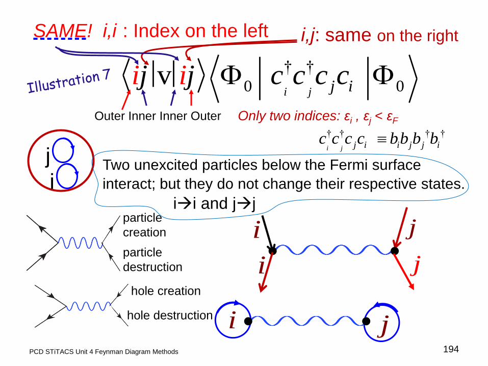
ji
i
i
194 PCD STiTACS Unit 4 Feynman Diagram Methods
† †
0 0v i j j ij j c c c ci i
i,j: same on the right SAME! i,i : Index on the left
Only two indices: εi , εj < εF
† † † † i j j i i j j ic c c c bb b b
particle
creation
particle
destruction
hole creation
hole destruction
j
j
Outer Inner Inner Outer
i
j Two unexcited particles below the Fermi surface
interact; but they do not change their respective states.
ii and jj

195 PCD STiTACS Unit 4 Feynman Diagram Methods
ji
εi , εj < εF
First order Direct or
Coulomb term
1
,
,
1 v v
2
i j i
i jE ij ij ij ji
No. of closed loops, λ=2
No. of hole lines, µ=2
41 1 1

† †
0 0v i j i jj i c c c ci j
j
i
196 PCD STiTACS Unit 4 Feynman Diagram Methods
j,i: on the right SAME! i,j : Index on the left
Only two indices: εi , εj < εF
hole creation
hole destruction
j
i
Outer Inner Inner Outer
Two unexcited particles below
the Fermi surface interact; and
they exchange their respective
states: ij and ji
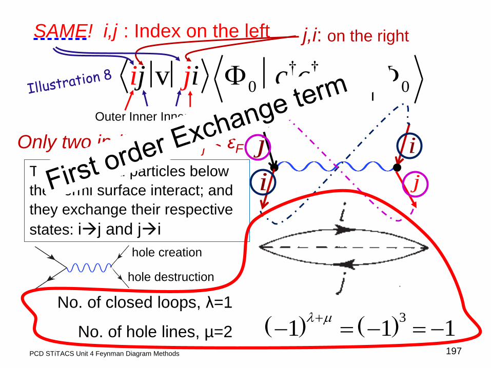
† †
0 0v i j i jj i c c c ci j
j
i
197 PCD STiTACS Unit 4 Feynman Diagram Methods
j,i: on the right SAME! i,j : Index on the left
Only two indices: εi , εj < εF
hole creation
hole destruction
j
i
Outer Inner Inner Outer
Two unexcited particles below
the Fermi surface interact; and
they exchange their respective
states: ij and ji
No. of closed loops, λ=1
No. of hole lines, µ=2 31 1 1

198 PCD STiTACS Unit 4 Feynman Diagram Methods
† † † †
0 0 .... i j i jk l k lc c c c c c c c
nth order term has the vacuum-vacuum
matrix element:
Its possible values are 0, +1, -1,
no matter what n
If for a Feynman graph, the no. of closed loops = λ,
and the no. of hole lines = µ,
then the contribution of this graph to < > is given by
1
Proof: based on Wick’s theorem

199 PCD STiTACS Unit 4 Feynman Diagram Methods
nA nth order term has
the vacuum-
vacuum matrix
element:
1 2
, , , , , , , , ,
2 2
....
1 2
....2
v
v
....
v
1
.... 1
1....
....
n
n
i j k l p q r s u w x y
n
n
i n t
n
i
ij lk
pq sr
uw yx
i n
i
e
i n
† † † † † †0 0
....i j pk l q r s u w x yc c c c c c c c c c c c

200 PCD STiTACS Unit 4 Feynman Diagram Methods
1 2 3
, , , , , , , , ,
3
† † † †01 2 3
2 3
3
2
v
v
v
3
1
2
1
i j p
n
i j k l p q r s u w x y
i t
k l q r
i
ij lk
pq sr
uw yx
e
i c c c c c c c c
i
i
† † 0s u w x yc c c c
3 A 3rd order term has
the vacuum-
vacuum matrix
element:

201 PCD STiTACS Unit 4 Feynman Diagram Methods
Raimes
Many Electron Theory Page 126 3rd order graphs ↑ t
Linked and Unlinked Graphs

202 PCD STiTACS Unit 4 Feynman Diagram Methods
Raimes Linked and Unlinked Graphs
Many Electron Theory Page 126 3rd order graphs ↑ t

203 PCD STiTACS Unit 4 Feynman Diagram Methods
Raimes Linked and Unlinked Graphs
Many Electron Theory Page 126 3rd order graphs ↑ t

204 PCD STiTACS Unit 4 Feynman Diagram Methods

205 PCD STiTACS Unit 4 Feynman Diagram Methods

206 PCD STiTACS Unit 4 Feynman Diagram Methods
0 .. 1,2,..DHF i i ih V u u i N
1 1 1 1
From STiAP U4L23/S119
( ) ( ) ( ) = i HF i i if r u q V u q u q
1 1
2
( )
(1) .. .. .. ( )
(1) .. .. .. ..1
.. .. .. .. |!
.. .. .. .. ..
(1) .. .. .. ( )
N
N N
u u N
u
N iN
u u N
2
0 ( 1, 1)Ze
h p m cr
Hartree-Fock Eq
Relativistic
Dirac-Hartree-Fock Eq
Relativistic Random Phase Approximation - RRPA W.R.Johnson and C.D.Lin Phys.Rev.A Vol.20,No.3, Sept. 1979
From STiAP
U3L14/S64

PCD STiTACS
Unit 4 Feynman Diagram Methods
207

208 PCD STiTACS Unit 4 Feynman Diagram Methods
( )
1 1
2
(1) .. .. .. ( )
(1) .. .. .. ..1
.. .. .. .. |!
.. .. .. .. ..
(1) .. .. .. ( )
N
N N
u u N
u
N iN
u u N
1
n m
n m
n m
ˆ uiG (r) (r)u
ˆ uF (r) (r)r
1 1
2 2
1 1
2 2
1
2
2
2
'
'
j , m m
j m
j , m m
for j
j mˆY (r)
j
j mˆY (r)
j
1 1
2 2
1 1
2 2
1
2
1
2 2
1
2 2
'
'
j , m m
j m
j , m m
for j
j mˆY (r)
j
j mˆY (r)
j
From STiAP: U3L18 / Slides 266, 267
Johnson & Lin Phys Rev A 1979

PCD STiTACS Unit 4 Feynman Diagram Methods 209
0
............... 1,2,..
DHF i i ih V u u
i N
Relativistic
Dirac-Hartree-Fock Eq
32
1
( ) [( ) ( ) ]
| |
N
DHF j j j j
j
d rV u r e u u u u u u
r r

( ) ( ) ( ) ( ) ...,i t i ti i i iu r u r w r e w r e
1 1
2
( )
(1) .. .. .. ( )
(1) .. .. .. ..1
.. .. .. .. |!
.. .. .. .. ..
(1) .. .. .. ( )
N
N N
u u N
u
N iN
u u N
v v i t i te e
Application of a
time-dependent
external field
with v , A †
and v v results in
higher harmonics↑
If we rebuild the (Time-Dependent) Dirac-Hartree-Fock
scheme with all the higher harmonics, we get NON-LINEAR
TIME-DEPENDENT DIRAC-HARTREE-FOCK Equations.

(1)
0( ) (v )i i i ij j
j
h V w V u u 1,2,..., .i N
211 PCD STiTACS Unit 4 Feynman Diagram Methods
Expanding TD-DHF equations in powers of the
external field, and retaining only first order terms, we get Linearized TD-DHF equations:
(1)
32
1
( )
[( ) ( ) ( ) ( ) ]| |
i
N
j j i j j i j i j j i j
j
V u r
d re u w u w u u w u u u u w
r r
maintain orthogonality of perturbed orbitals
with the occupied orbitals
ij
jw
( )iu r
Lagrange multipliers
↑DHF potential
includes electron-electron correlations
L-TD-DHF

212 PCD STiTACS Unit 4 Feynman Diagram Methods
(1)
32
1
( )
[( ) ( ) ( ) ( ) ]| |
i
N
j j i j j i j i j j i j
j
V u r
d re u w u w u u w u u u u w
r r
(1)
0( ) ( v )i i i ij j
j
h V w V u u ↑ driving terms
(1)
0( ) ;i i i ij j i
j
h V w V u u w 1,2,..., .i N
Basic RRPA equations are obtained by dropping the
‘driving’ terms
1,2,..., .i N
i
i
w
w
: Positive frequency components final state correlations
: Negative frequency components initial state correlations
B-RRPA
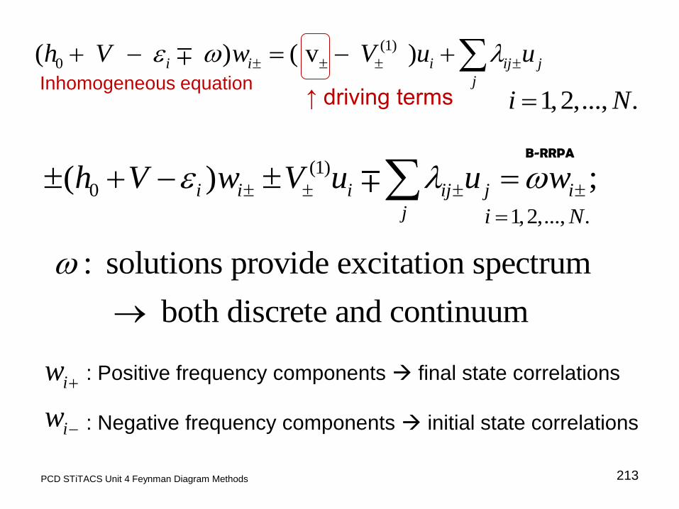
213 PCD STiTACS Unit 4 Feynman Diagram Methods
(1)
0( ) ( v )i i i ij j
j
h V w V u u ↑ driving terms 1,2,..., .i N
i
i
w
w
: Positive frequency components final state correlations
: Negative frequency components initial state correlations
(1)
0( ) ;i i i ij j i
j
h V w V u u w 1,2,..., .i N
B-RRPA
Inhomogeneous equation
: solutions provide excitation spectrum
both discrete and continuum

214 PCD STiTACS Unit 4 Feynman Diagram Methods
We solve the L-TD-DHF equations in terms of the
solutions of the B-RRPA equations.
3 † †
1
v vN
i i i i
i
T e d r w u w u
Transition amplitude from the initial state to an
excited state described by the RRPA functions
of frequency induced by
is given by:
iw
v v i t i te e

PCD STiTACS Unit 4 Feynman Diagram Methods 215

216 PCD STiTACS Unit 4 Feynman Diagram Methods
Relativistic Quantum
Theory of Atoms
and Molecules,
I.P.Grant
Ch.9.10
Fig.9.8
time
Time
forward
ring
diagram
Time
forward
exchange
diagram
Time
backward
exchange
diagram
Time
backward
ring
diagram
Uncorrelated
matrix
element
217 PCD STiTACS Unit 4 Feynman Diagram Methods

218 PCD STiTACS Unit 4 Feynman Diagram Methods Questions: [email protected]
https://www.physics.iitm.ac.in/~labs/amp/
Walter R.Johnson | with Vojislav Radojevic | with Steven T. Manson
RRPA ; R-MCTD
Radojevic,Gagan Pradhan, PCD, Karan Govil,Jobin Jose,S.Sunil Kumar, N.M.Murty, N.Shanthi, H.Chakraborty, Alak Banik, Aarthi Ganesan, Ashish Kumar, Tanima Banerjee, Hari Varma, Ankur Mandal, Soumyajit Saha, K.Sindhu
time