Feynman Path Integral: rigorous formulation · M. Beau, Feynman Path Integral approach to electron di raction for one and two slits, analytical results , Eur. J. Phys. 33 (2012) Mathieu

Feynman Path Integral : an overviewThomas-Bijma-Dorlas-Beau approach

Conclusions

Feynman Path Integral:rigorous formulation

Mathieu Beau, Postdoctoral researcherDublin Institut for Advanced Studies (DIAS)

Collaborator : Prof. Tony Dorlas, DIAS

Mathieu Beau, Postdoctoral researcher Dublin Institut for Advanced Studies (DIAS)Feynman Path Integral: rigorous formulation


Conclusions

Summary :

1. Feynman Path Integral : from a calculus to a rigorousdefinition

2. A rigorous Approach (Thomas-Bijma, Dorlas-Beau) :path distribution

3. Conclusions et perspectives



Conclusions

Quantum mechanics and path integralIntegral CalculusRigorous Approaches : non-exhaustive list

1. Feynman Path Integral :from a calculus to a rigorous definition



Conclusions


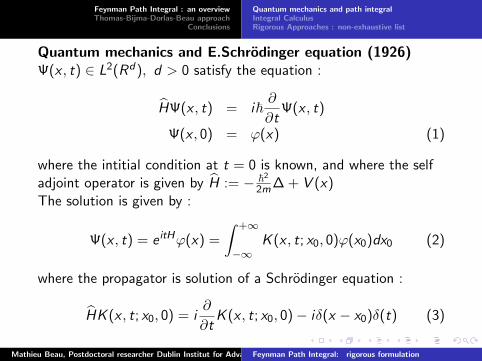
Quantum mechanics and E.Schrodinger equation (1926)Ψ(x , t) ∈ L2(Rd), d > 0 satisfy the equation :

HΨ(x , t) = i~∂

∂tΨ(x , t)

Ψ(x , 0) = ϕ(x) (1)

where the intitial condition at t = 0 is known, and where the selfadjoint operator is given by H := − ~2

2m∆ + V (x)The solution is given by :

Ψ(x , t) = e itHϕ(x) =

∫ +∞

−∞K (x , t; x0, 0)ϕ(x0)dx0 (2)

where the propagator is solution of a Schrodinger equation :

HK (x , t; x0, 0) = i∂

∂tK (x , t; x0, 0)− iδ(x − x0)δ(t) (3)



Conclusions


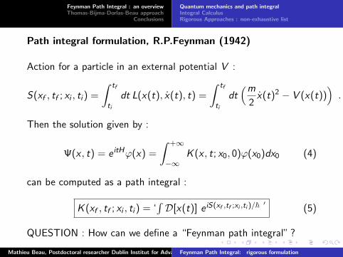
Path integral formulation, R.P.Feynman (1942)

Action for a particle in an external potential V :

S(xf , tf ; xi , ti ) =

∫ tf

ti

dt L(x(t), x(t), t) =

∫ tf

ti

dt(m

2x(t)2 − V (x(t))

).

Then the solution given by :

Ψ(x , t) = e itHϕ(x) =

∫ +∞

−∞K (x , t; x0, 0)ϕ(x0)dx0 (4)

can be computed as a path integral :

K (xf , tf ; xi , ti ) = ‘∫D[x(t)] e iS(xf ,tf ;xi ,ti )/~ ′ (5)

QUESTION : How can we define a “Feynman path integral” ?



Conclusions


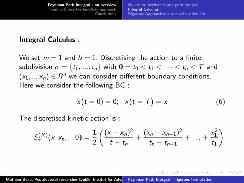
Integral Calculus :

We set m = 1 and ~ = 1. Discretising the action to a finitesubdivision σ = t1, ..., tn with 0 = t0 < t1 < · · · < tn < T and(x1, .., xn) ∈ Rn we can consider different boundary conditions.Here we consider the following BC :

x(t = 0) = 0; x(t = T ) = x (6)

The discretised kinetic action is :

S (K)σ (x , xn, .., 0) =

1

2

((x − xn)2

t − tn+

(xn − xn−1)2

tn − tn−1+ . . .+

x21

t1

)



Conclusions


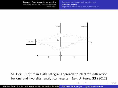
2b

2a

z

x

LD

Source

Slits Screen

M. Beau, Feynman Path Integral approach to electron diffractionfor one and two slits, analytical results , Eur. J. Phys. 33 (2012)



Conclusions


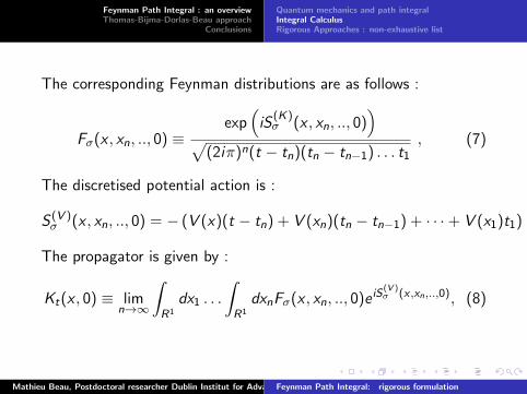
The corresponding Feynman distributions are as follows :

Fσ(x , xn, .., 0) ≡exp

(iS

(K)σ (x , xn, .., 0)

)√

(2iπ)n(t − tn)(tn − tn−1) . . . t1

, (7)

The discretised potential action is :

S (V )σ (x , xn, .., 0) = − (V (x)(t − tn) + V (xn)(tn − tn−1) + · · ·+ V (x1)t1)

The propagator is given by :

Kt(x , 0) ≡ limn→∞

∫R1

dx1 . . .

∫R1

dxnFσ(x , xn, .., 0)e iS(V )σ (x ,xn,..,0), (8)



Conclusions


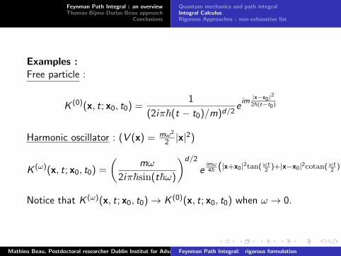
Examples :Free particle :

K (0)(x, t; x0, t0) =1

(2iπ~(t − t0)/m)d/2eim|x−x0|

2

2~(t−t0)

Harmonic oscillator : (V (x) = mω2

2 |x|2)

K (ω)(x, t; x0, t0) =

(mω

2iπ~sin(t~ω)

)d/2

eimω4~ (|x+x0|2tan(ωt

2)+|x−x0|2cotan(ωt

2))

Notice that K (ω)(x, t; x0, t0)→ K (0)(x, t; x0, t0) when ω → 0.



Conclusions


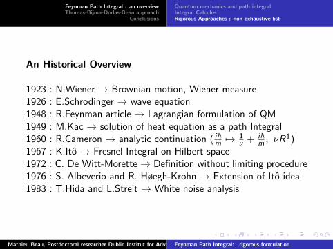
An Historical Overview

1923 : N.Wiener → Brownian motion, Wiener measure1926 : E.Schrodinger → wave equation1948 : R.Feynman article → Lagrangian formulation of QM1949 : M.Kac → solution of heat equation as a path Integral1960 : R.Cameron → analytic continuation ( i~m 7→

1ν + i~

m , νR1)1967 : K.Ito → Fresnel Integral on Hilbert space1972 : C. De Witt-Morette → Definition without limiting procedure1976 : S. Albeverio and R. Høegh-Krohn → Extension of Ito idea1983 : T.Hida and L.Streit → White noise analysis



Conclusions


Principle interests

1976 : K. Ito, S. Albeverio and R. Høegh-Krohn → Fresnel Integralon Hilbert space

1983 : T.Hida and L.Streit → White noise analysis

2000 : E. Thomas → Path distribution on sequence spaces



Conclusions


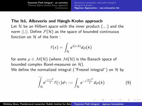
The Ito, Albeverio and Høegh-Krohn approachLet H be an Hilbert space with the inner product (., .) and thenorm ||.||. Define F(H) as the space of bounded continuousfonction on H of the form :

f (x) =

∫H

e i(x ,k)dµ(k)

for some µ ∈M(H) (where M(H) is the Banach space ofbounded complex Borel-measures on H).We define the normalized integral (“Fresnel integral”) on H by∫

He i||γ||2

2 f (γ)dγ :=

∫H

e−i||k||2

2 dµ(k) (9)



Conclusions


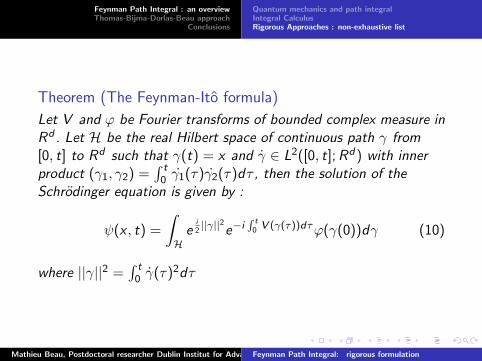
Theorem (The Feynman-Ito formula)

Let V and ϕ be Fourier transforms of bounded complex measure inRd . Let H be the real Hilbert space of continuous path γ from[0, t] to Rd such that γ(t) = x and γ ∈ L2([0, t]; Rd) with innerproduct (γ1, γ2) =

∫ t0 γ1(τ)γ2(τ)dτ , then the solution of the

Schrodinger equation is given by :

ψ(x , t) =

∫H

ei2||γ||2e−i

∫ t0 V (γ(τ))dτϕ(γ(0))dγ (10)

where ||γ||2 =∫ t

0 γ(τ)2dτ



Conclusions


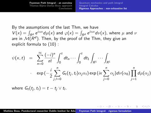
By the assumptions of the last Thm, we haveV (x) =

∫Rd e iαxdµ(x) and ϕ(x) =

∫Rd e iαxdν(x), where µ and ν

are in M(Rd). Then, by the proof of the Thm, they give anexplicit formula to (10) :

ψ(x , t) =∞∑n=0

(−i)n

n!

∫ t

0dtn · · ·

∫ t

0dt1

∫R1

· · ·∫R1

· exp (− i

2

n∑j ,l=0

Gt(tj , tl)αjαl) exp (ixn∑

j=0

αj)dν(α0)n∏

j=1

dµ(αj)

where Gt(tj , tl) = t − tj ∨ tl .



Conclusions


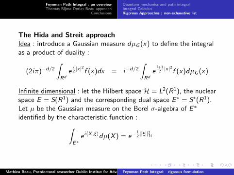
The Hida and Streit approachIdea : introduce a Gaussian measure dµG (x) to define the integralas a product of duality :

(2iπ)−d/2

∫Rd

ei2|x |2f (x)dx = i−d/2

∫Rd

ei+1

2|x |2f (x)dµG (x)

Infinite dimensional : let the Hilbert space H = L2(R1), the nuclearspace E = S(R1) and the corresponding dual space E ∗ = S∗(R1).Let µ be the Gaussian measure on the Borel σ-algebra of E ∗

identified by the characteristic function :∫E∗

e i〈X ,ξ〉dµ(X ) = e−12||ξ||2H



Conclusions


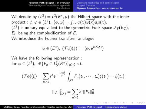
We denote by (L2) = L2(E ∗, µ) the Hilbert space with the innerproduct : φ, ϕ ∈ (L2), (φ, ϕ) =

∫E∗ φ(x)ϕ(x)dµ(x).

(L2) is unitary equivalent to the symmetric Fock space FS(EC ),EC being the complexification of E .We introduce the Fourier-transform analogue

φ ∈ (E ∗), (T φ)(ξ) := 〈φ, e i〈X ,ξ〉〉

We have the following representation :for ϕ ∈ (L2), ∃!Fn ∈ L2

S(Rn)n≥0 s.t.

(T φ)(ξ) =∑n≥1

ine−||ξ||20

2

∫Rn

Fn(t1, · · · , tn)ξ(t1) · · · ξ(tn)

||ϕ||2(L2) =∑n≥0

n!||Fn||20



Conclusions


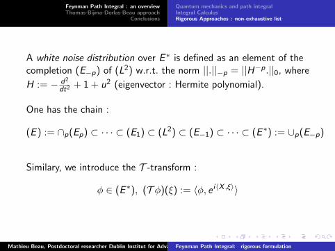
A white noise distribution over E ∗ is defined as an element of thecompletion (E−p) of (L2) w.r.t. the norm ||.||−p = ||H−p.||0, where

H := − d2

dt2 + 1 + u2 (eigenvector : Hermite polynomial).

One has the chain :

(E ) := ∩p(Ep) ⊂ · · · ⊂ (E1) ⊂ (L2) ⊂ (E−1) ⊂ · · · ⊂ (E ∗) := ∪p(E−p)

Similary, we introduce the T -transform :

φ ∈ (E ∗), (T φ)(ξ) := 〈φ, e i〈X ,ξ〉〉



Conclusions


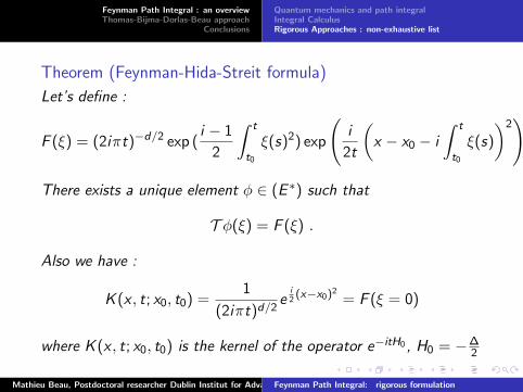
Theorem (Feynman-Hida-Streit formula)

Let’s define :

F (ξ) = (2iπt)−d/2 exp (i − 1

2

∫ t

t0

ξ(s)2) exp

(i

2t

(x − x0 − i

∫ t

t0

ξ(s)

)2)

There exists a unique element φ ∈ (E ∗) such that

T φ(ξ) = F (ξ) .

Also we have :

K (x , t; x0, t0) =1

(2iπt)d/2e

i2

(x−x0)2= F (ξ = 0)

where K (x , t; x0, t0) is the kernel of the operator e−itH0 , H0 = −∆2



Conclusions


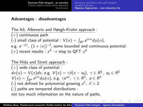
Advantages - disadvantages

The Ito, Albeverio and Høegh-Krohn approach :(+) continuous path(-) small class of potential : V (x) =

∫Rd e iαxdµ(α),

e.g. e−|x |, (1 + |x |)−2, some bounded and continuous potential.(+) recent results : x4 → step to QFT φ4

The Hida and Streit approach :(+) wide class of potential :dν(x) = V (x)dx , e.g. V (x) = γδ(x − x0), γ ∈ R1, x0 ∈ R1

V (x) =∫Rd eαxdµ(α), e.g. γeax , γ ∈ R1, a ∈ R1

(-) not defined for polynomial growing xδ, δ > 2(-) paths are tempered distributions :not too much information on the nature of paths.



Conclusions

ProgramFeynman-Thomas measure and distribution on Rn

Feynman-Thomas measure and distribution on l2γResults - discussion

2. A rigorous Approach (Thomas-Bijma, Dorlas-Beau) :path distribution



Conclusions



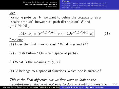
Idea :For some potential V , we want to define the propagator as a“scalar product” between a “path distribution” F and

e−i∫ t

0 V [x(t)] :

Kt(x , x0) ≡ 〈e−i∫ t

0 V [x(t)],F 〉 = 〈De−i∫ t

0 V [x(t)], µ〉 (11)

Problems :(1) Does the limit n→∞ exist ? What is µ and D ?

(2) F distribution ? On which space of paths ?

(3) What is the meaning of 〈·, ·〉 ?

(4) V belongs to a space of functions, which one is suitable ?

This is the final objective but we first want to look at thediscrete-time analogue → not easy to do and a lot to understand



Conclusions



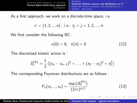
As a first approach, we work on a discrete-time space, i.e.

σ = 1, 2, .., n, i .e. tj = j = 1, 2, ..., n

We first consider the following BC :

x(0) = 0; x(n) = 0 (12)

The discretised kinetic action is :

S (K)σ =

1

2

((xn − xn−1)2 + . . .+ (x2 − x1)2 + x2

1

)The corresponding Feynman distributions are as follows :

Fσ(x1, .., xn) =exp (iS

(K)σ )

(2iπ)n/2(13)



Conclusions



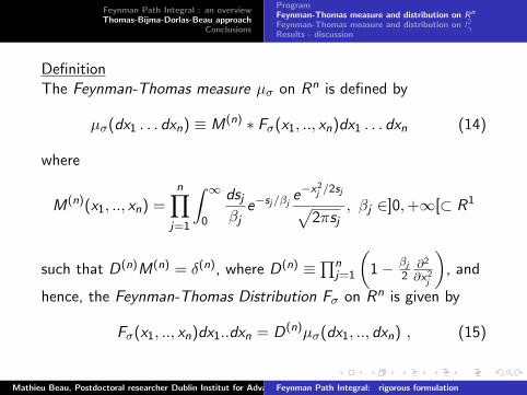
DefinitionThe Feynman-Thomas measure µσ on Rn is defined by

µσ(dx1 . . . dxn) ≡ M(n) ∗ Fσ(x1, .., xn)dx1 . . . dxn (14)

where

M(n)(x1, .., xn) =n∏

j=1

∫ ∞0

dsjβj

e−sj/βje−x

2j /2sj√

2πsj, βj ∈]0,+∞[⊂ R1

such that D(n)M(n) = δ(n), where D(n) ≡∏n

j=1

(1− βj

2∂2

∂x2j

), and

hence, the Feynman-Thomas Distribution Fσ on Rn is given by

Fσ(x1, .., xn)dx1..dxn = D(n)µσ(dx1, .., dxn) , (15)



Conclusions



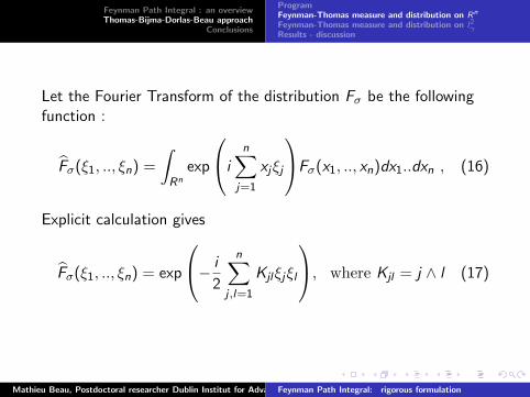
Let the Fourier Transform of the distribution Fσ be the followingfunction :

Fσ(ξ1, .., ξn) =

∫Rn

exp

in∑

j=1

xjξj

Fσ(x1, .., xn)dx1..dxn , (16)

Explicit calculation gives

Fσ(ξ1, .., ξn) = exp

− i

2

n∑j ,l=1

Kjlξjξl

, where Kjl = j ∧ l (17)



Conclusions



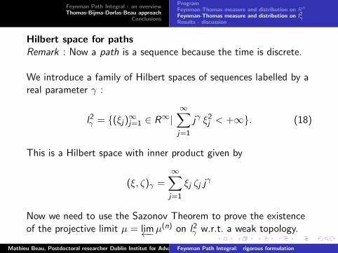
Hilbert space for pathsRemark : Now a path is a sequence because the time is discrete.

We introduce a family of Hilbert spaces of sequences labelled by areal parameter γ :

l2γ = (ξj)∞j=1 ∈ R∞|

∞∑j=1

jγ ξ2j < +∞. (18)

This is a Hilbert space with inner product given by

(ξ, ζ)γ =∞∑j=1

ξj ζj jγ

Now we need to use the Sazonov Theorem to prove the existenceof the projective limit µ = lim←−µ

(n) on l2γ w.r.t. a weak topology.



Conclusions



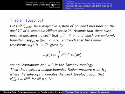
Theorem (Sazonov)

Let (µ(n))n∈N1 be a projective system of bounded measures on thedual H′ of a separable Hilbert space H. Assume that there existpositive measures νn such that |µ(n)| ≤ νn and which are uniformlybounded : supn∈N1 ||νn|| < +∞, and such that the Fouriertransforms Φn : H → C 1 given by

Φn(ξ) =

∫e i〈ξ, x〉νn(dx),

are equicontinuous at ξ = 0 in the Sazonov topology.Then there exists a unique bounded Radon measure µ on H′σ,where the subscript σ denotes the weak topology, such thatπ′n(µ) = µ(n) for all n ∈ N1.



Conclusions



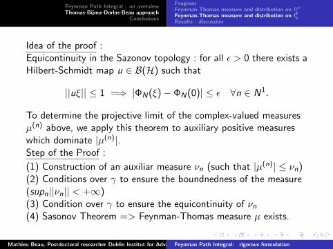
Idea of the proof :Equicontinuity in the Sazonov topology : for all ε > 0 there exists aHilbert-Schmidt map u ∈ B(H) such that

||uξ|| ≤ 1 =⇒ |ΦN(ξ)− ΦN(0)| ≤ ε ∀n ∈ N1.

To determine the projective limit of the complex-valued measuresµ(n) above, we apply this theorem to auxiliary positive measureswhich dominate |µ(n)|.Step of the Proof :

(1) Construction of an auxiliar measure νn (such that |µ(n)| ≤ νn)(2) Conditions over γ to ensure the boundnedness of the measure(supn||νn|| < +∞)(3) Condition over γ to ensure the equicontinuity of νn(4) Sasonov Theorem => Feynman-Thomas measure µ exists.



Conclusions



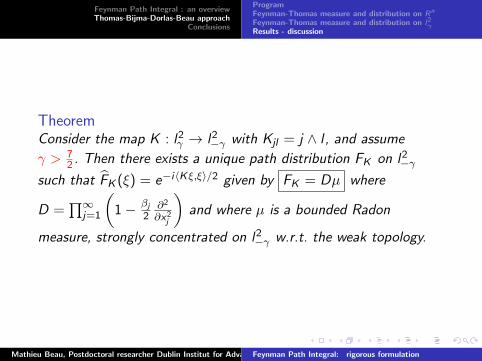
TheoremConsider the map K : l2

γ → l2−γ with Kjl = j ∧ l , and assume

γ > 72 . Then there exists a unique path distribution FK on l2

−γsuch that FK (ξ) = e−i〈Kξ,ξ〉/2 given by FK = Dµ where

D =∏∞

j=1

(1− βj

2∂2

∂x2j

)and where µ is a bounded Radon

measure, strongly concentrated on l2−γ w.r.t. the weak topology.



Conclusions



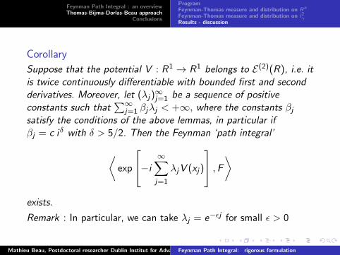
Corollary

Suppose that the potential V : R1 → R1 belongs to E(2)(R), i.e. itis twice continuously differentiable with bounded first and secondderivatives. Moreover, let (λj)

∞j=1 be a sequence of positive

constants such that∑∞

j=1 βjλj < +∞, where the constants βjsatisfy the conditions of the above lemmas, in particular ifβj = c iδ with δ > 5/2. Then the Feynman ‘path integral’

⟨exp

−i∞∑j=1

λjV (xj)

,F⟩

exists.

Remark : In particular, we can take λj = e−εj for small ε > 0



Conclusions



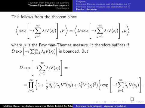
This follows from the theorem since⟨exp

−i∞∑j=1

λjV (xj)

,F⟩ =

⟨D exp

−i∞∑j=1

λjV (xj)

, µ⟩

where µ is the Feynman-Thomas measure. It therefore suffices if

D exp[−i∑∞

j=1 λjV (xj)]

is bounded. But

D exp

−i∞∑j=1

λjV (xj)

=

=∞∏j=1

1 +

1

2βj(iλjV

′′(xj) + λ2j V ′(xj)

2)

exp

−i∞∑j=1

λjV (xj)

.



Conclusions



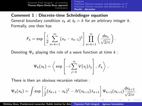
Comment 1 : Discrete-time Schrodinger equationGeneral boundary condition xk at t0 = k for an arbitrary integer k .Formally, one then has

Fk = exp

[i

2

∞∑n=k+1

(xn − xn−1)2

] ∞∏n=k+1

(dxn√2iπ

).

Denoting Ψk playing the role of a wave function at time k :

Ψk(xk) =

⟨exp

−i∞∑j=k

V (xj)λj

, Fk

⟩,

There is then an obvious recursion relation :

Ψk(xk) =

∫exp

[i

2(xk+1 − xk)2 − iV (xk+1)λk+1

]Ψk+1(xk+1)

dxk+1√2iπ

.



Conclusions



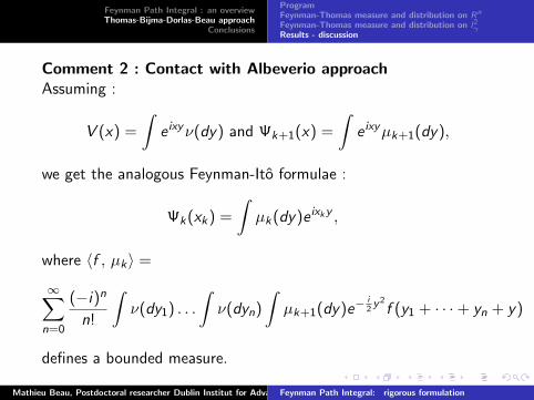
Comment 2 : Contact with Albeverio approachAssuming :

V (x) =

∫e ixyν(dy) and Ψk+1(x) =

∫e ixyµk+1(dy),

we get the analogous Feynman-Ito formulae :

Ψk(xk) =

∫µk(dy)e ixky ,

where 〈f , µk〉 =

∞∑n=0

(−i)n

n!

∫ν(dy1) . . .

∫ν(dyn)

∫µk+1(dy)e−

i2y2

f (y1 + · · ·+ yn + y)

defines a bounded measure.



Conclusions



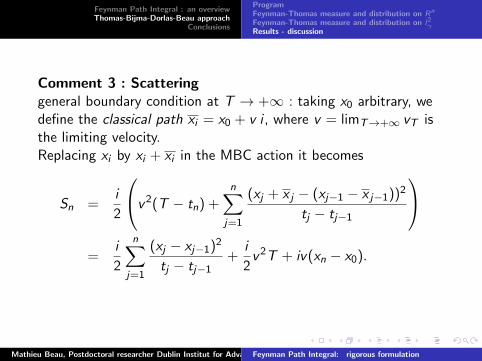
Comment 3 : Scatteringgeneral boundary condition at T → +∞ : taking x0 arbitrary, wedefine the classical path xi = x0 + v i , where v = limT→+∞ vT isthe limiting velocity.Replacing xi by xi + xi in the MBC action it becomes

Sn =i

2

v 2(T − tn) +n∑

j=1

(xj + x j − (xj−1 − x j−1))2

tj − tj−1

=

i

2

n∑j=1

(xj − xj−1)2

tj − tj−1+

i

2v 2T + iv(xn − x0).



Conclusions



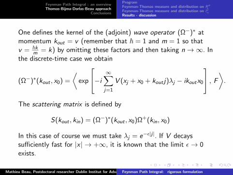
One defines the kernel of the (adjoint) wave operator (Ω−)∗ atmomentum kout = v (remember that ~ = 1 and m = 1 so thatv = ~k

m = k) by omitting these factors and then taking n→∞. Inthe discrete-time case we obtain

(Ω−)∗(kout , x0) =

⟨exp

−i∞∑j=1

V (xj + x0 + kout j)λj − ikoutx0

, F

⟩.

The scattering matrix is defined by

S(kout , kin) = (Ω−)∗(kout , x0)Ω+(kin, x0)

In this case of course we must take λj = e−ε|j |. If V decayssufficiently fast for |x | → +∞, it is known that the limit ε→ 0exists.



Conclusions



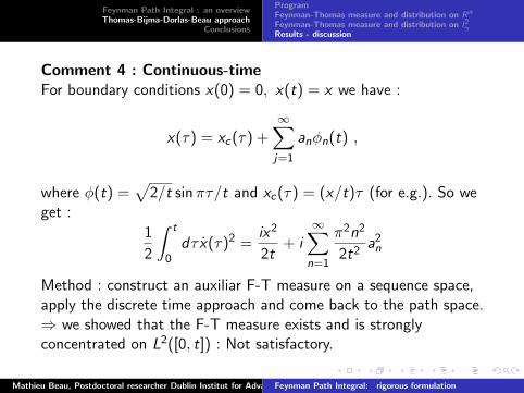
Comment 4 : Continuous-timeFor boundary conditions x(0) = 0, x(t) = x we have :

x(τ) = xc(τ) +∞∑j=1

anφn(t) ,

where φ(t) =√

2/t sinπτ/t and xc(τ) = (x/t)τ (for e.g.). So weget :

1

2

∫ t

0dτ x(τ)2 =

ix2

2t+ i

∞∑n=1

π2n2

2t2a2n

Method : construct an auxiliar F-T measure on a sequence space,apply the discrete time approach and come back to the path space.⇒ we showed that the F-T measure exists and is stronglyconcentrated on L2([0, t]) : Not satisfactory.



Conclusions

3. Conclusions and future projects



Conclusions

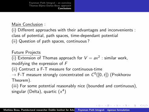
Main Conclusion :(i) Different approaches with their advantages and inconvenients :class of potential, path spaces, time-dependant potential(ii) Question of path spaces, continuous ?

Future Projects(i) Extension of Thomas approach for V = ax2 : similar work,modifying the expression of F(ii) Contruct a F-T measure for continuous-time→ F-T measure strongly concentrated on C 0([0, t]) (ProkhorovTheorem).(iii) For some potential reasonably nice (bounded and continuous),singular (Delta), quartic (x4)



Conclusions

Interests(I) Wide applications : scattering theory, diffraction theory,magnetic field, semi-classical approximation, time dependent Gibbsstates , QFT(II) Statistical Mechanics : Feynman-Kac Integral (fermion, boson,polymers)(III) Pure Mathematics : Infinite dimensional analysis, EDP.



Conclusions

References

- S. A. Albeverio and R. Høegh-Krohn, Mathematical Theory ofFeynman Path Integrals. Springer Lecture Notes in Mathematics523, 1976.- T. Hida et L.Streit, White Noise : An infinite dimensionalcalculus. Kluwer, Dordrecht (1995)- E. Thomas, Path distributions on sequence spaces. Proc. Conf.on Infinite-dimensional Stoch. Anal. Neth. Acad. Sciences, 1999,235–268.- M. Beau, T. Dorlas, Discrete-Time Path Distributions on HilbertSpace, Indagationes Mathematicae 24, 212-228 (2012)[arXiv :1202.2033]


Documents

Feynman Path Integral: rigorous formulation · M. Beau, Feynman Path Integral approach to electron di raction for one and two slits, analytical results , Eur. J. Phys. 33 (2012) Mathieu