Embed Size (px)
Citation preview

Mechanical characterisation of fibres for engineered wood products: A scanning force microscopy study
S. Fernando1, C.F. Mallinson1, C. Phanopolous2, D.A. Jesson1* and J.F. Watts1
1Centre for Engineering Materials, Department of Mechanical Engineering Sciences, University of
Surrey, Guildford, Surrey, GU2 7XH, UK
2Huntsman Polyurethanes, Everslaan 45, 3078 Everberg, Belgium
*Corresponding Author: [email protected], Tel 01483 686299; Fax: 01483 686291
Abstract
Mechanical properties of individual wood fibres and the characterisation of the interaction between
wood fibres and resins are of interest to the composite wood panel industry and others involved in the
fabrication of engineered wood products. However, the size of such fibres typically a few millimetres
in length, makes characterisation of their mechanical properties difficult. Gripping fibres is
problematic, not to mention the measurement of meaningful load displacement data. Using a novel
three point bend test technique, the Young’s moduli of single wood fibres were determined. Fibres
were placed on a specially designed test rig and a scanning probe microscope was used to apply a load
and to measure the deflection at the centre of each fibre. A model of the fibre was produced in order to
facilitate data analysis. The technique proved to be feasible, resulting in an average Young’s modulus
value of 24.4 GPa for Pinus Sylvestris softwood fibres. This compares well with other values in the
literature, but there is scope for improvement in the methodology to lead to more accurate
measurements.
Keywords: AFM, Flexure, Stiffness, Wood Fibre
1. IntroductionNatural fibres are (potentially) environmental-friendly alternatives to synthetic fibres: they are
abundant and renewable. Composites made of natural fibres, which continue to use a synthetic
polymer matrix, have the advantage of being able to maintain the formability and stability of the
polymer matrix. In the current market, everyday household consumer products such as furniture and
automotive parts are fabricated using natural fibre composites. Other potential areas include aerospace,
marine and construction industries [1].
1

A significant issue with natural fibres remains the inconsistency in performance, which arises from
natural variability in cross-sectional area and microstructure [2-4]. However, breaking fibres into
smaller fragments or constituent parts can overcome this issue to at least some extent. A particular
example of this is wood, which can be broken down in several ways, including into single cells.
Wood fibres, are generally elongated hollow wood cells that exist in both softwood and hardwood. In
softwoods such as Scots Pine (Pinus Slyvestris), fibre lengths range from 2 to 6 mm and have widths
of 20 to 40 µm. The cells also contain pits. The pits form part of the water transport system since they
control the passage of moisture from one cell to the next [5, 6]. Wood fibres are produced by
defibrillation. Wood chips are soaked in water and heated to 100 oC for several minutes to soften
them. They are then charged into a refiner, which is effectively two counter rotating profiled metal
discs or plates of approximately 30 cm radius: in the refiner the fibres are at very high pressures and
temperatures. The wood chips move from the centre of the plates to the edges during which time they
are gradually reduced to bundles and then single fibres. At the point where the fibres depart the plates,
they experience a very sudden drop in pressure and most bundles of wood fibres that are still intact
explosively decompress to fibres. There are usually a range of fibre qualities that result, including
residual fibre bundles or shrieves, truncated fibres and wood dust. After the decompression step the
fibres are usually still at around 10 bars pressure and ca 180 oC. They are then conveyed to a hot air
dryer to remove most of the moisture down to approximately 8-12% moisture content and then cooled
to room temperature before storage.
Mechanical properties of individual wood fibres and the characterisation of the interaction between
wood fibres and resins are of interest to the composite wood panel industry. Composite wood
products, such as medium density fibreboard, are comprised of individual wood fibres with polymer
resins as binders. Compared with glass or carbon fibre reinforced polymer composites, where the
volume fraction of resin is typically ~40 % of the product, here the resin is used at a much smaller
proportion of the product. The resins typically constitute 5-15 % of the materials used to produce a
panel, dependent on the residual moisture content of the wood. The final composition can see this
number reduced significantly: sometimes the resin comprises as a little as 2% of the volume of the
panel, due to the presence of trapped air. Wood fibres account for more than 85% of natural fibres
commercially extracted in the world [7]. Over 80% of natural fibre composites are comprised of
wood fibres [8].
The current work presents details of a novel test methodology to determine mechanical properties of
wood fibres, which can be used to inform and improve computational models and in order to compare
the effects of various treatments. Following this introduction, a brief background to the nature of
wood fibres is presented, together with details of some of the previous attempts to measure mechanical
2

properties. This is followed by a section on the experimental methodology and the development of a
jig used in the current work. Results and a discussion of these are presented and the Concluding
Remarks include some thoughts on potential improvements to the methodology.
2. Background Wood cell walls, as shown in Fig. 1, is comprised of a primary wall (P), and three secondary cell walls
(S1, S2 and S3) [6]. Each of these walls has a different configuration of cellulose microfibrils. The
tensile strength and Young’s modulus of wood fibres are largely dependent on the S2 layer as it
accounts for about 80% of the total cell wall thickness [9, 10]. The average (total) cell wall thickness
for Scot Pine samples has been found to be 2.0 µm in the earlywood region and 3.8 µm in the
latewood region [11].
Fig. 1 A schematic diagram showing the three-dimensional structure of the cell wall of a tracheid
Previous methodologies employed to characterise the mechanical properties of wood fibre aggregates
can be divided into three general groups: i) tensile testing; ii) nano-indentation; and iii) other. With
any of these techniques, the major difficulty lies in handling the fibres and interpreting the output. A
brief summary of these three approaches and the results arising therefrom is presented here.
Tensile TestingUniversal testing machines (UTMs) fitted with small vice grips have been used in several studies
conducted in the 1960s to determine the mechanical properties of individual wood fibres [9]. Problems
associated with direct uniaxial tensile are with regards to gripping the fibres, such as fibre slippage
3

because of insufficient gripping force and the unquantifiable effect of compressing cell walls within
the grips. To overcome this, attempts were made to glue the fibres to paper or plastic tabs, and
consequently clamping the paper tabs within the vice grips. Although this method was an
improvement, it had its own drawbacks such as the tedious and time-consuming nature of the process
of manipulating the fibres, gluing them in such a way that kept the adhesive from penetrating into the
cell wall of the fibre (which in turn would compromise the mechanical properties of the fibre, and, in
addition, the resin can also spread over the surface of the fibre which will equally compromise the
mechanical properties [9].
A limit for a proportional stress-strain relationship of single wood fibres in tension was found in early
studies [12]. There were attempts made to relate the ultrastructure (that is to say the structure within
the cell) to mechanical properties. Such research showed that the tensile Young’s modulus of spruce, a
type of softwood, fibres are between approximately 20 GPa and 80 GPa, depending on the microfibril
angles within the S2 layer of each fibre. It was found that the tensile Young’s modulus reduces with
increasing microfibril angles [13]. Previous work also highlighted that the moisture content of the
fibres should be controlled, as it has an effect on mechanical properties [9].
Nano-indentationResearch utilising nano-indentation techniques has been performed using wood samples which were
sectioned through the transverse plane which exposed the cross-sections of each fibre. This enabled an
indenter to indent the secondary cell wall in the longitudinal direction of each fibre within the sample
section of wood. This technique enabled the use of a model of elastic contact, such as the Derjaguin-
Muller-Toporov (DMT) model, to calculate the local elastic modulus from load-displacement curves
produced [14]. Using this technique, the Young’s modulus of the secondary cell wall of spruce was
found to be 13.5 GPa for cell walls in the earlywood region and 21.0 GPa for those in the latewood
region. Although samples were taken from several growth rings, the study did not investigate the
relationship between the microfibril angle and the Young’s modulus [14]. However, a nano-
indentation study conducted on loblolly pine stem found that the Young’s modulus increases with
decreasing microfibril angles [15].
Other TechniquesScanning force microscopy (SFM) can be used to assess the local mechanical properties of materials
and has previously been employed to quantify the local elastic modulus of an epoxy impregnated
hardened cement paste. The technique produces force-separation curves which are comparable to load-
displacement curves provided by UTMs. However, the study states that the equipment needed to be
calibrated thoroughly to obtain quantitatively reliable outcomes [16]. SFM has also been used to
measure the Young’s Modulus of amyloid fibrils, and found that the results were in agreement with an
4

indirect evaluation of fibrils stiffness that was obtained by combining topological statistical analysis
and polymer physics [17].
The common feature of these SFM techniques is that they work by pressing a fine tip, mounted on the
end of a cantilever arm, into the sample; this effectively deforms the sample locally. Similar to classic
nano-indentation techniques, this enables the use of a model of elastic contact, such as the DMT
model, to calculate the local elastic modulus of the samples.
Atomic force microscopy (AFM), a type of SFM, has been used in a cantilever bend test to determine
the Young’s modulus of a spruce wood cell wall [18]. In this study, a focused ion beam (FIB) was
used to prepare wood cell wall samples with rectangular cross-sections. One end of each sample was
fixed and a force was applied in increments to the other end using the AFM tip. The force applied was
measured directly by the AFM, whilst the displacement was measured using automated image analysis
of micrographs acquired during the tests. These, combined with cantilever bending equations, enabled
the Young’s modulus of the cell wall in bending to be calculated. A summary of the properties
determined by the methods outlined above is given in Table 1.
Table 1 Table highlighting the Young’s moduli of different wood types obtained from various engineering test methods
obtained from the literature
Softwood Type Test Type E / GPa ReferenceDouglas Fir, Average Tensile test 24 [19]Spruce Tensile test 20 - 80 [13]Loblolly Pine, Earlywood Tensile test 14.8 [20]Loblolly Pine, Latewood Tensile test 19.7 [20]Spruce, Earlywood Nano-indentation 13.5 [14]Spruce, Latewood Nano-indentation 21 [14]Loblolly Pine, Latewood Nano-indentation 14 [15]Spruce , Average Nano-indentation 16.1 [10]Wood Fibre - General n/a 18 - 40 [7]Spruce Cell wall in cantilever bending 22 [18]
3. Experimental MethodsA sample of fibres produced by the method indicated in section 1 was used for the study. This was a
commercially produced mixed softwood fibre ‘furnish’ which was mainly pinus sylvestris (Scots
Pine). From this sample, a set of single, intact fibres was extracted using fine point tweezers.
Reflected light microscopy (RLM) and scanning electron microscopy (SEM) were used to assess a
small sub-set of the group, as shown in Fig 2, in order to measure fibre dimensions and to investigate
if there were any other structural characteristics of the fibres which would affect the mechanical
property measurement methodology.
5
Fig. 2 Example micrographs: a) RLM micrograph showing a single fibre b) SEM digital micrograph showing the location of
pits
Following an initial feasibility study, the use of an atomic force microscope (AFM, specifically a
Bruker Dimension Edge), one of a family of SFM methods, to perform a three point bend test, was
chosen as the most suitable technique as the method does not involve clamping the fibres at the ends.
To facilitate a three point bend test, a test jig was designed, with two supports 2 mm apart. The jig was
designed to accommodate each fibre in the configuration illustrated in Fig. 3a. This enabled a force to
be applied, using AFM, onto the mid-point of each fibre whilst the ends of the fibre rested on pivots.
An example of the AFM tip engaged on an individual wood fibre is shown in Fig. 3b.
Fig. 3 Three point bend test: a) Schematic diagram of the set-up and b) an optical image of the AFM tip engaged on a wood
fibre (top-view – the white arm is pressing down on the fibre).
The AFM tip used for the experiments had a stiffness of 11.7 N m-1, a value which was measured
internally following the calibration of the AFM. After mounting the fibre on the test rig, optical
microscopy was utilised to measure the length of the fibres between the pivots, which were typically -
2 mm when normal to the knife edge. The delicate nature of handling the fibres meant that they could
6

not always be placed perpendicular to the pivot edge, thus making it essential to measure the distance
between the pivots, as opposed to treating it as a constant value.
The test rig with the mounted fibres was then placed on the AFM mounting plate. Firstly, the AFM
optical view was used to check that both ends of the fibre were resting on the pivots. NanoDrive
V8.05 software controls were then used to move the mounting plate as required to position the AFM
cantilever tip above the centre of one of the fibres mounted on the rig. Once positioned as required, the
tip was engaged onto the fibre. After the tip successfully engaged with the fibre, the Point
Spectroscopy function was used to apply a bending force. This was performed by specifying
displacement limits for the cantilever tip movement, consequently applying a bending force. The
cantilever tip was displaced at a constant rate of 50 nm s -1, and the maximum amount displaced was
always kept to under 1 µm. This process was repeated three times for each fibre.
Using the Bruker NanoScope V1.5 data analysis software, the deflection signal of the AFM cantilever
arm, in units of force, was plotted against the ‘Z position’ of the arm. The ‘Sensitivity’ and ‘Spring
Constant’ values were updated to those determined during the calibration of the AFM cantilever arm.
Doing so provided an output graph which was representative of the force-displacement behaviour of
the sample under test.
The graphs from the AFM display regions of significant adhesion forces arising when the tip comes
into and out of contact with the sample, as shown in Fig. 4. Adding to that, wood fibres appeared to
show hysteresis and a degree of non-linear, and non-elastic behaviour. Therefore, the gradient of the
best fit line from the linear region of each graph was measured instead of the ‘peak applied force’ and
the ‘total deflection of the fibre’ under bending. The gradient, K, was recorded for both the loading
(extend) and unloading (retract) curves of the AFM force-displacement plot. In addition, temperature
and humidity levels of the laboratory were monitored during the tests.
7

Fig. 4 Force-displacement graph obtained using the point spectroscopy AFM function on an individual wood fibre. The
regions of particular analytical interest are labelled
A model for beam bending of a fibre was developed. This was based on a scenario of a fibre being
treated as an annulus of uniform wall thickness and of the fibre in three point bending. A full analysis
of the model is presented in Appendix A. This then gives rise to Equation 1, from which E can be
determined: a value of 3 µm was used for the fibre wall thickness in the beam bending model.
E= 148
L3
IK Equation 1
Where,
E = Young’s modulus
L = Distance between pivots
I = Second moment of area of the cross-section
K = Bending stiffness
The wood pulp was stored for 48 hours prior to testing in the laboratory where the three point bend
tests were conducted (i.e. at ambient temperature and humidity). A selection of fibres from the pulp
was used to measure the average moisture content. This was achieved using a TA Laboratories SDT-
Q600, capable of performing thermogravimetric analysis (TGA) and differential scanning calorimetry
(DSC) simultaneously. TGA analysis provides a measurement of the weight change as a sample is
heated, while DSC provides a measurement of the heat flow. The empty sample holder was first
placed in the instrument, and the weight reading was set to zero. A selection of fibres was then placed
on the holder. The sample was heated from room temperature up to 600 ºC. The instrument recorded
the change in weight with increasing temperature.
8

4. Results and DiscussionResults of the mechanical tests are presented in Table 2 and it can be seen that the loading and
unloading curve results are in good agreement.
Table 2 Summary of the results obtained from the three-point bending tests performed on the 9 wood fibres in this study.
Values for the loading and unloading AFM curves are shown
Unloading LoadingFibre I / µm4 K / N m-1 E/ GPa K / N m-1 E/ GPaFibre 1 24639 4.55 43.2 4.73 44.9Fibre 2 53523 4.04 18.1 3.69 16.6Fibre 3 36712 4.38 30.2 4.45 30.7Fibre 4 20528 2.39 26.3 2.22 24.6Fibre 5 49116 5.18 25.5 4.86 23.9Fibre 6 31319 3.28 25.9 2.95 23.3Fibre 7 18772 2.03 20.7 1.88 19.1Fibre 8 49961 2.84 11.5 2.62 10.7Fibre 9 61878 5.53 17.8 5.16 16.6
The chart shown in Fig. 5 compares the Young’s moduli of tested fibres to values found in the
literature (as summarised in Table 2). The results of the unloading curve are used in this comparison.
Microfibril angles of cell walls have a significant impact on the Young’s modulus of a fibre. In fact,
softwood fibres showed a decrease in the measured Young’s modulus with increasing microfibril
angle values [20]. This may explain the results as the Young’s modulus values vary from 11.5 GPa to
43.2 GPa. The temperature of the laboratory was between 18 ºC and 22 ºC. The relative humidity of
the laboratory was between 30% and 60%. The moisture content of uncoated wood fibres was 5.3% of
the total fibre weight, from TGA.
9

Fig. 5 Young's moduli comparison for each of the examined wood fibres (x axis values correspond to a specific fibre) in this
study together with values obtained from the literature
Generally, the Young’s moduli are within the range for softwood fibres found in previous work, as
seen in Fig. 5. However, in addition to the fact that previous work on fibre properties of Pinus
Sylvestris fibres could not be found, not all the previous research specifically state the moisture
content of the fibres tested. It should also be noted that in the current work the fibre selection process
did not discriminate between specific fibre types such as early or late wood, heart or sap wood,
longitudinal or ray cells, reaction wood - this also leads to variability which could be somewhat
reduced by careful selection. Further, it can also be argued whether the results from the nano-
indentation tests and the AFM cantilever bending test can be used for comparison, because those
studies involved just the cell walls of fibres as opposed to complete, separated single fibres. A
combination of these reasons makes it difficult for a direct comparison to be made between results of
this study and previous work. It is also highlighted that the three point bend tests were performed
using an AFM cantilever arm which did not have the ideal stiffness range required for the tests as
suggested within the literature [18].
10

Bending stiffness values from the unloading force-displacement SFM curves were treated as the ‘final
results’. This is because previous research involving nano-indentation techniques used gradients of
unloading curves to determine the Young’s moduli. It is also seen that there is no significant
difference between the values obtained from the loading and unloading curves.
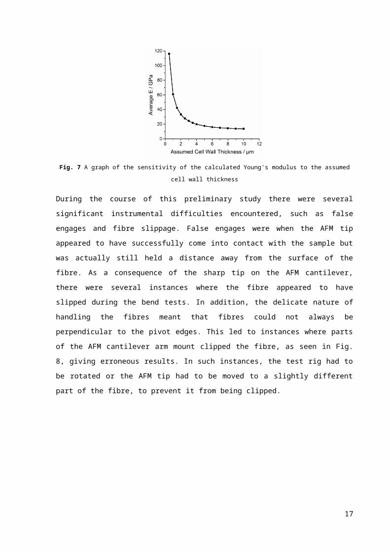
The beam bending model used in the study assumed a constant wall thickness of 3 µm based upon
previous research [11]. However, SEM digital micrographs of fibre cross-sections, as seen in Fig. 6,
show the extent of difference in wall thickness hence confirming the presence of both earlywood and
latewood fibres, and indeed different fibre types. Given the difference in wall thicknesses, a sensitivity
analysis was undertaken to investigate the effect of varying wall thickness on the Young’s modulus
values reported in this work. Fig. 7 shows the sensitivity of the average calculated Young’s modulus
values of fibres to the value of the wall thickness used in the beam-bending model. The analysis
reveals that the different wall thicknesses found in this study would only have a minor impact on the
values reported herein.
Fig. 6 SEM digital micrographs of individual wood fibre cross sections from a) Earlywood b) Latewood
Fig. 7 A graph of the sensitivity of the calculated Young's modulus to the assumed cell wall thickness
11

During the course of this preliminary study there were several significant instrumental difficulties
encountered, such as false engages and fibre slippage. False engages were when the AFM tip appeared
to have successfully come into contact with the sample but was actually still held a distance away
from the surface of the fibre. As a consequence of the sharp tip on the AFM cantilever, there were
several instances where the fibre appeared to have slipped during the bend tests. In addition, the
delicate nature of handling the fibres meant that fibres could not always be perpendicular to the pivot
edges. This led to instances where parts of the AFM cantilever arm mount clipped the fibre, as seen in
Fig. 8, giving erroneous results. In such instances, the test rig had to be rotated or the AFM tip had to
be moved to a slightly different part of the fibre, to prevent it from being clipped.
Fig. 8 Optical image from the AFM viewing camera showing a problem encountered during the work. A white arrow
highlights the position at which the fibre is being clipped by the cantilever support chip during a measurement
Fibres appeared to show hysteresis, along with a degree of non-linear and non-elastic behaviour.
Hence, only the linear regions of the loading and unloading curves were used to measure the bending
stiffness (gradient of the linear region). An example of this is shown in Fig. 9.
Fig. 9 A force-displacement graph obtained using the point spectroscopy AFM function on an individual wood fibre. The
graph highlights non-linear behaviour of a wood fibre
12

Once the tip had successfully engaged with the fibre, three consecutive readings were taken and the
results were only considered as valid if all three force-displacement graphs were consistent. If they
were not, the whole process was repeated again. This was performed as a way of ensuring that the
AFM results were correct and reliable.
The AFM requires thorough calibration in order to obtain quantitatively reliable outcomes [16]. The
stiffness of the AFM cantilever arm needs to be higher than the stiffness of the sample under test. In
fact, previous research used a cantilever arm with a stiffness which was two orders of magnitude
higher than that of the specimen under test [18]. This was so that the deflection of the arm is negligible
compared to the deflection of the specimen, hence giving accurate results. Although the cantilever arm
used was calibrated thoroughly, the stiffness of the arm was found to be 11.7 N m-1. The bending
stiffness of all fibres tested were approximately between 2 and 6 N m-1. Therefore, it is clear that the
cantilever arm used was not the two orders of magnitude higher than the fibres that is recommended
for work of this type. To address this, attempts were made to calibrate readily available cantilever
arms of marked stiffness values of 26 N m-1 and 40 N m-1. However, the calibration procedure for
those arms was unsuccessful. Therefore, it was decided that the option of using a thoroughly calibrated
arm of a lower stiffness was favourable over using an uncalibrated arm of a higher indicated stiffness.
The use of a sharp AFM tip raised the question as to whether the fibre surface was being indented as
opposed to the entirety of the fibre being in three-point bending. To ensure this was not the case the
AFM tip was used to apply a force onto the fibre at a point just above one of the pivots. The gradients
of the resulting force-displacement curves were approximately 9 N m-1 which is not within the range
for the bending stiffness results of the fibres tested in three point bending (2 - 6 N m-1). This was also a
concern raised in previous work from this laboratory, where a similar AFM technique was used to
examine the mechanical properties of amyloid fibrils [21].
Ideally, to obtain more accurate results, a tipless cantilever arm of stiffness value of at least 600 N m-1
should be used. The use of a tipless cantilever arm would help prevent issues such as false engages
and fibre slippage. However, tipless cantilevers with such high stiffness values are not readily
available, although the removal of a tip by focussed ion beam milling is clearly a possibility.
The most significant contribution to the uncertainties of the Young’s Modulus results is believed to be
the measurement uncertainty of the mid-section diameter measurements as the fibres are irregular. The
SEM digital micrographs of fibre cross-sections showed that the fibres are not circular in cross-
section, even though the beam bending model used to calculate the Young’s moduli assumed an
annulus cross-section. Also, the fibres appear to twist along their length which means that the
‘diameters’ measured using reflective light microscopy could be either a width of a cell wall or the
13

diagonal width. (This could be a natural phenomenon in some fibres, but also could be due to the
moisture content, the moisture history and the rates of change of moisture content. These will all be
different for different qualities of fibres even if exposed to the same ambient conditions. For example,
heart wood is more hydrophobic than sap wood and would therefore experience less movement due to
ambient moisture variation). This is in addition to the general variation of widths along the fibre
length. These factors lead to high measurement uncertainties associated with the average mid-section
diameters.
5. Concluding Remarks
The primary objective of this study was to develop a methodology which would enable the mechanical
properties of a single wood fibre to be determined accurately. This was achieved using a three point
bend test in an AFM. Although the three point beam bending model relied on the assumption that the
fibre cross-section was a perfect annulus with a constant wall thickness, values for the Young’s
modulus were obtained from a number of fibres which matched the existing literature.
In reviewing the performance of the experiment and the results obtained, three particular issues have
been noted. Firstly, it is essential to use an AFM cantilever arm with a bending stiffness which is
significantly greater than the bending stiffness of the wood fibres. Secondly, in handling the fibres, it
became apparent that the natural propensity for the fibre to curl slightly within a volume, rather than
lying flat, causes some issues during mechanical testing. However, in bending methodologies, the
usual minimum span-length between the two pivot points is taken as 10 times the depth of the
specimen. On this basis it would be possible to reduce the span to 400-500 μm, which should reduce
the problem of the fibre becoming displaced. Finally, the mathematical model has been shown to be
idealised. This is not a particular issue per se, particularly when used for making comparisons, but
there are a number of opportunities to develop the model further, including correction factors for
variations in wall thickness and eccentricity in the fibre cross section.
Several modifications to the experimental set-up and analysis to improve the quality of results that can
be obtained from this method are possible. These include: examining cross-sections of several fibres to
tailor the equation for the second moment of area, as opposed to assuming the cross-section of a fibre
to be an annulus with a constant wall thickness. This would require extensive use of SEM to observe
fibre cross-sections of a large number of wood fibres to determine the best possible model to use. This
has been tried in the past, where the ‘true’ cross-sectional areas of jute fibres was determined using
digital image analysis and compared models where the fibres cross-sections were assumed to be
perfectly circular or elliptical [20]. A FIB could be used to remove the tip from a commercially
14

available AFM cantilever with a sufficient stiffness so that it would not deflect during the
measurement.
AcknowledgementsThe authors would like to thank Mr Steve Bowers and colleagues in the Faculty Workshop for assistance in the manufacture of the jig used in the current work, and Mr Dave Jones and Miss Rebecca Tung from Surrey’s MicroStructural Studies Unit for assistance with RLM and SEM.
Compliance with Ethical Standards:The authors declare that there is no conflict of interest associated wth the current work.
References
[1] Thakur V, Thakur M, Singha A, (2013) Biomass-based Biocomposites. Shawbury, UK: Smithers Rapra Technology Ltd.
[2] Jesson, D.A, Gobin, V.P.T., Gallagher, S., Smith P.A. and Watts J.F. “Properties of Natural Fibres for Composite Materials”, Proceedings of the 17th International Conference on Composite Materials, [2009] Edinburgh, UK
[3] Chard, J.M., Creech, G., Jesson, D A, Smith, P A, “Green Composites: Sustainability and Mechanical Performance”, Polymers, Rubbers and Composites, 42, (2013) 421-426
[4] Virk A, Hall W, Summerscales J, (2010). Physical Characterization of Jute Technical Fibers. Journal of Natural Fibres 7: (3), 216-228.
[5] Hacke U, Sperry J, Pittermann J, (2004) Anaylsis of Circular Bordered Pit Function II. Gymnosperm Tracheids with Torus-margo Pit Membranes. Am J Bot 91: (3), 386-400.
[6] Ansell M, (2015) Wood Microstructure - A Cellular Composite. In: M. Ansell, ed. Wood Composites Engineering with Wood - From Nanocellulose to Superstructures. Cambridge: Woodhead Publishing Limited, pp 1-27.
[7] Dai D, Fan M, (2014) Wood fibres as reinforcements in natural fibre composites: structure, properties, processing and applications. In: A. H. a. R. Shanks, ed. Natural fibre composites: Materials, Processes and Properties. Philadelphia, PA: Woodhead Publishing Limited, pp 3-41.
[8] Shah D, Schubel PJ, Clifford M, Licence P, (2013) Fatigue life evaluation of aligned plant fibre composites through S-N curves and constannt-life diagrams. Compos Sci Technol 74: 139-149.
[9] Mott L, (1995) Micromechanical Properties and Fracture Mechanics of Single Wood Pulp Fibers: a PhD Thesis. University of Maine
[10] Gindl W, Gupta H, (2002) Cell-Wall Hardness and Young's Modulus of Melamine-Modifed Spruce Wood by Nano-indentation. Compos Part A-Appl S 33: 1141-1145.
15

[11] Havimo M, Rikala J, Sirviö J, Sipi M, (2009) Tracheid Cross-sectional Dimensions in Scots Pine (Pinus Sylvestris) - Distributions and Comparison with Norway Spruce (Picea abies). Silva Fenn 43: (4), 681-688.
[12] Jayne BA, (1959) Mechanical Properties of Wood Fibers. TAPPI 42: (6), 461-467.
[13] Page D, E-Hosseiny F, Winkler K, Lancaster A, (1977). Elastic Modulus of Single Wood Pulp Fibers. TAPPI 60: (4), 114-117.
[14] Wimmer R, Lucas BN, Tsui TY, Oliver WC, (1997) Longitudinal Hardness and Young's of Spruce Tracheid Secondary Walls Using Nano-indentation Technique. Wood Sci Technol 31: 131-141.
[15] Tze W, Wang S, Rials TG, Pharr GM, Kelley SS, (2007) Nano-indentation of Wood Cell Walls: Continuous Stiffness and Hardness Measurements. Compos Part A-Appl S 38: (3), 945-953.
[16] Trtik P, Kaufmann J, Volz U, (2012) On The Use of Peak-Force Tapping Atomic Force Microscopy for Quantification of the Local Elastic Modulus in Hardened Cement Paste. Cement and Concrete Res 42: (1), 215-221.
[17] Adamcik J, Berquand A, Mezzenga R, (2011) Single-step Direct Measurement of Amyloid Fibrils Stiffness by Peak Force Quantitative Nanomechanical Atomic Force Microscopy. Appl Phys Lett 98: 193701.
[18] Orso S, Wegst U, Arzt E, (2006) The Elastic Modulus of Spruce Wood Cell Wall Material Measured by an In Situ Bending Technique. J Mater Sci 41: (16), 5122-5126.
[19] Kersavage PC, (1973) A System for Automatically Recording the Load-elongation Characteristics of Single Wood Fibers Under Controlled Relative Humidity Conditions. United States Department of Agriculture : US Government Printing Office.
[20] Mott L, Groom L, Shaler S, (2002) Mechanical Properties of Individual Southern Pine Fibers. Part II: Comparison of Earlywood and Latewood Fibers with respect to Tree Height and Juvenility. Wood Fiber Sci 34: (2), 221-237.
[21] Flamia R, Zhdan PA, Castle JE, Tamburro AM, (2008) Comment on the mechanical properties of the amyloid fibre, poly(ValGlyGlyLeuGly), obtained by a novel AFM methodology. J Mater Sci 43: (1), 395-397.
16
Appendix C
AppendicesA – Beam Bending Model The beam bending model for a beam under symmetric three point bending with unconstrained ends, as shown in Fig. A1, was considered to be the most applicable model to be used in the study.
Fig. A1 Symmetric three point bending
The bending moment, M, is −Fx
2 . This can be substituted into elastic beam bending equation given in
Equation A1.
EI d2 yd x2 =M Equation A1
Where,E = Young’s modulus of the beam materialM = Bending momentI = Second moment of area of the beam cross-section
The resulting equation can be integrated as shown to produce an equation for the deflection of the beam, y, in terms of the distance from the end, x, the distance between the pivots, L, the Young’s modulus, E, and the second moment of area of the beam cross-section, I (Equation A2).
EI d2 yd x2 =
−Fx2
EI dydx
=−F x2
4+c1
At x= L2 ,
dydx
=0. Therefore c1=F L2
16 .
EI dydx
=−F x2
4+ F L2
16
EIy=−F x3
12+ F L2 x
16+c2
At x=0, y=0. Therefore c2=0 .
17

EIy=−F x3
12+ F L2 x
16
y= FxEI ( L2
16− x2
12 )y= Fx
48 EI(3 L2−4 x2)
The deflection at the centre of the beam, δ , is the value of y when x= L2 :
δ= F L3
48 EIEquation A2
Where,E = Young’s modulus of the beam materialL = Distance between pivotsI = Second moment of area of the beam cross-sectionF = Applied forceδ = Total deflection of the beam
The basic beam bending equation presented above assumes that the beam displays linear elastic behaviour during the application of the bending force and that the deflection is small (proportionally to the size of the specimen). Force-displacement graphs from the AFM display regions of significant adhesion forces. Wood fibre samples also appeared to show hysteresis and a degree of non-linear and non-elastic behaviour. Therefore, the gradient of the best fit line from the linear region of each curve was measured instead of the ‘peak applied force’ and the ‘total deflection of the fibre’ under bending. This gradient, K, is the bending stiffness (Equation A3). Factoring in this gradient leads a modified three point bend equation specific to this study (Equation A4).
K= ΔFδ Equation A3
Where,K = Bending stiffnessΔF = Change in applied forceδ = Deflection corresponding to ΔF
E= 148
L3
IK Equation A4
Where,E = Young’s modulusL1 = Distance between pivotsI = Second moment of area of the cross-sectionK = Bending stiffness
For simplicity, it was assumed that the cross-section of an uncoated wood fibre was in the shape of an annulus, as shown in Fig. A2. It was also assumed that the fibre cross-section was constant along the length of the fibre. This allowed the following equation to be used to calculate the second moment of area (Equation A5):
18
I=π4(r1
4−r 24) Equation A5
Where,I = Second moment of area r1 = Outer radiusr2 = Inner radius
Fig. A2 - Illustration of an annulus
The equation was modified to be more specific to the study by writing r1 and r2, in terms of the average outer mid-section diameter, Avg D, and the wall thickness of a fibre (Equation A6).
I=π4(( Avg D
2 )4
−( Avg D2
−t)4
) Equation A6
Where,I = Second moment of area of the fibre cross-section Avg D = Average mid-section diameter of the fibre t = Wall thickness of the fibre
19


![Abstractepubs.surrey.ac.uk/853893/1/manuscript 03.03.20.docx · Web view2003/03/20 · This includes suicide, common mental health disorders and alcohol abuse [5,9–11]. That said,](https://img.pdfslide.net/doc/110x75/5f2a3e8f8d8854158d3fc77e/030320docx-web-view-20030320-this-includes-suicide-common-mental-health.jpg)

![Undergraduate Writing Assignments in Mechanical Engineering...Mechanical Engineering, Electrical and Computer Engineering, Biosystems Engineering, Civil Engineering and Design Engineering]](https://img.pdfslide.net/doc/110x75/5ff7a06f83bfbd5c864bdc1a/undergraduate-writing-assignments-in-mechanical-engineering-mechanical-engineering.jpg)