Embed Size (px)
Citation preview
Fictitious Pricing in Retail
Donald Ngwe∗
March 7, 2016
Abstract
Prices in a wide variety of contexts come in three parts: an “original” or “suggested” price,
a discount off that price, and the final price. Little empirical evidence is available that speaks
to how each pricing component affects purchase behavior, even as theories abound. This paper
outlines the main theories of fictitious pricing with their corresponding predictions and examines
their relevance empirically. It exploits retail transactions data that features large variations in
these pricing components together with a relatively homogeneous product space. The results
have important implications for how managers should set each pricing component to maximize
profits.
1 Introduction
Virtually all firms engage in some form of discount pricing. There are several reasons for which
firms might drop the price of a good over time, such as when it seeks to discriminate between
consumers according to their willingness to pay, as a means of managing its inventory, or when
it faces less demand uncertainty after the good’s introductory phase. In many of these instances,
consumers can be thought of as having nearly full information and making rational responses to
price incentives. This work, on the other hand, focuses on motivations for discount pricing that arise
from consumers having imperfect information, or possibly exhibiting irrational behavior. These are
∗E-mail: [email protected]. This paper is based on a chapter of my dissertation. I am grateful to my dissertationcommittee members Chris Conlon, Brett Gordon, Kate Ho, Michael Riordan, and Scott Shriver for their guidanceand advice.
1
motivations that might encourage firms to post high “original” prices at which products are never
actually available for purchase.
In this paper, I identify patterns in how consumers respond to discounts. I use data from a dominant
fashion goods retailer that makes heavy use of this strategy in its outlet stores. This data set offers
a rare opportunity to study this pricing strategy because it records both original and transacted
prices, as well as repeat purchases. A portion of these original prices are observably genuine, while
the remainder are suggested. As with most outlet stores, the firm implements random discounts
across both time and products in store, providing much variation in the transacted prices.
I find that consumer responses to suggested prices are consistent with several theories both of prices
as a signal of quality and of reference-dependent behavior. Controlling for transactional prices and
other product characteristics, a higher “original” price increases a good’s purchase probability.
While this effect is larger for products for which original prices are genuine, it is also substantial
for products with suggested original prices. Moreover, this effect seems to be invariant to the
consumer’s level of information.
Somewhat puzzlingly, this positive effect increases exponentially in the original price (and equiva-
lently, the discount amount). One might expect this effect to exhibit diminishing marginal returns
if consumers are less likely to put much stock in overly inflated original prices. In addition, optimal
behavior by firms would suggest concave returns to higher suggested prices since increasing these
prices is costless. I find that reference dependence offers a partial explanation of this phenomenon.
Consumers take the average discount level in a store as the reference point, and are more likely to
purchase goods that are more highly discounted than this benchmark.
This reference dependence is in line with the idea that firms exploit bargain-hunting behavior
through suggested pricing. This effect may be particularly potent in outlet stores, in which most
items are discounted. Yet the attractiveness of a bargain must go hand-in-hand with original prices
being a reliable signal of quality. This implies that the firm must maintain the credibility of these
prices even as it employs them to manipulate consumer behavior.
Setting suggested prices is a unique problem for the firm, as suggested prices can be thought of as a
signal of quality akin to certain forms of advertising. Yet unlike advertising, setting higher suggested
2
prices is costless to the firm. Setting optimal suggested prices, therefore, involves balancing their
(initially) demand-enhancing effects versus the possibility that consumers may eventually lend less
credibility to these signals.
This chapter proceeds as follows. Section 2 reviews the related literatures on pricing and reference
dependence. Section 3 describes the data used for the empirical analysis and provides some de-
scriptive statistics. Section 4 outlines a demand model and presents parameter estimates. Section
5 concludes and points to directions for future work.
2 Related literature
Suggested pricing can occur in a wide variety of circumstances. The environment I consider has
the following features: a single seller that produces goods of varying quality, a weak regulatory
environment, consumers that have less information than the firm about product quality and past
prices, and the possibility of repeat purchases. An additional, novel characteristic is that the
marginal cost of production may not be monotonically increasing with quality. This occurs, for
instance, in the manufacture of fashion goods for which the attractiveness of the final product may
have little relationship with the processes involved in its production.
Several authors have recognized the importance of price as a signal of quality for uninformed
consumers. Bagwell and Riordan (1991) argue that high and declining prices can indicate that a
product is of high quality. In their framework, high prices are a credible signal of quality because
high quality, high-cost firms are more willing to restrict sales volume than low-cost firms. Over
time, as the proportion of uninformed consumers decreases, it becomes easier for the high-cost firm
to signal its quality and thus its price lowers toward the full-information monopoly price.
Armstrong and Chen (2013) examine a similar environment, but one in which quality is endoge-
nously determined and consumers can potentially be misled by false price announcements. They
find that when consumers are ignorant of the initial price, the firm finds it profitable to produce
a high quality good and announce the initial price when it is constrained to tell the truth. How-
ever, it does even better by producing a low quality good, and subsequently misleading consumers
3

by announcing a high initial price. Therefore, a key empirical question of particular interest to
regulators is: Are consumers deceived by suggested prices?
Results from behavioral economics provide additional and alternative explanations for why high
suggested prices might be effective in driving demand. Bordalo, Gennaioli and Shleifer (2013) argue
that salient attributes are overweighted by consumers when choosing between goods. They proceed
to show how this logic can explain “misleading sales,” which are mostly identical to what I term
suggested pricing. The difference is that retailers inflate original prices during misleading sales,
instead of maintaining the same false original price throughout a product’s lifetime.
Recently authors have begun to reconcile anomalous patterns in field data using concepts generated
in behavioral economics. One such example is Hastings and Shapiro (2012), who find that consumers
switch from premium to regular gasoline given a uniform price increase to an extent that cannot be
accounted for by wealth effects. They present this as evidence of mental accounting, which manifests
itself through the infungibility of money between an individual’s different purposes (Thaler 1985).
The above-mentioned theories frequently have conflicting predictions on both consumer behavior
and firm decisions, owing to difference in fundamental assumptions. Perhaps because of the rareness
of obtaining data with suggested prices, there has been no related empirical work on actual retail
settings. Thus, this is a valuable opportunity to test and measure the relative importance of analytic
results on both discount pricing and suggested pricing.
Models of price as a signal of quality and those of reference dependence have different predictions
of how consumers react to false list prices and provide different motivations for the firm to post
suggested prices. Following Bagwell & Riordan (1991) and Armstrong & Chen (2013), suppose that
a monopolist supplies one good over two periods, setting prices pt for periods t = 1, 2. Quality may
be high or low, with marginal costs being ci, i ∈ {H,L} respectively. Marginal costs are common
knowledge. Consumers are heterogeneous in their patience and there level of information about
the quality of the good. A portion x of consumers are trendy : they are eager to buy the good,
can ascertain its quality, and are in the market in period 1. The remaining 1− x of consumers are
casual : buyers who are uncertain about the good’s quality and enter the market in period 2.
In Bagwell & Riordan (1991), casual consumers do not observe the purchasing decisions of trendy
4
consumers, and the firm is constrained to set p1 = p2. Casual consumers infer product quality
from price, their knowledge of the firm’s cost function and the proportion of trendy consumers. If
x is small enough, and under equilibrium refinements, casual consumers accept a high price as a
credible signal of high quality. Over time, as x increases, the firm can signal high quality with less
effort, and thus high quality goods exhibit prices that are initially high but decline over time.
Armstrong & Chen (2013) relax the problem along several dimensions. First, the firm is allowed
to choose quality and set p1 6= p2. They show that if x is large enough, then the firm chooses to
provide high quality and set high prices in both periods if casual consumers do not observe p1. The
condition on x weakens when casual consumer can observe p1, which provides an incentive for the
firm to (credibly) inform casual consumers about past prices. However, when casual consumers
can be fooled into believing a false announcement about p1, then the firm maximizes its profits by
producing low quality goods, setting low prices in period 1, and misinforming casual consumers
about p1.
An alternative explanation of why suggested prices exist is provided by Bordalo et al. (2013). They
conceptualize salience as it applies to a discrete choice setting. Suppose the consumer’s choice set is
C ≡ (qj , pj)j=1,...,N . Each good j has quality qj and price pj . Without salience effects, a consumers
values good j with a utility function that assigns equal weights to quality and price:
uj = qj − pj .
Salient thinking, meanwhile, puts more weight on attributes that stand out for each good. Denote
by (q, p) the reference good consisting of average attributes q =≡∑
j qj/N and p =≡∑
j pj/N .
The salience of quality for good j is then σ(qj , q) and the salience of price is σ(pj , p).
The salience function σ(·, ·) is symmetric and continuous and satisfies the following conditions:
1. Ordering. Let µ = sgn(aj − a). Then for any ε, ε′ ≥ 0 with ε+ ε′ > 0, we have
σ(aj + µε, a− µε′) > σ(aj , a).
5

2. Diminishing sensitivity. For any aj , a ≥ 0 and all ε > 0, we have
σ(aj + ε, a+ ε) < σ(aj , a).
In choice set C, quality is salient for good j when σ(qj , q) > σ(pj , p), price is salient for good j
when σ(qj , q) < σ(pj < p), and price and quality are equally salient when σ(qj , q) = σ(pj , p).
An example of a salience function is
σ(aj , a) =|aj − a|aj + a
(1)
for aj , a 6= 0, and σ(0, 0) = 0.1
(Bordalo et al, 2013) The salient thinker’s evaluation of good j enhances the relative utility weight
attached to the salient attribute (keeping constant the sum of weights attached to quality and
price). Formally,
uSj =
2
1+δ · qj + 2δ1+δ · pj if σ(qj , q) > σ(pj , p)
2δ1+δ · qj + 2
1+δ · pj if σ(qj , q) < σ(pj , p)
qj − pj if σ(qj , q) = σ(pj , p)
where δ ∈ (0, 1] decreases in the severity of salient thinking.
Using the definitions in this subsection I illustrate how a demand model that incorporates salient
thinking would predict different purchase decisions from a standard demand model.
Let C1 = {(q0 = 0, p0 = 0), (q1 = 15, p1 = 3), (q2 = 20, p2 = 4)}. A non-salient thinker would
assign values u1 = 12 and u2 = 16, and would thus opt for the high-quality product. Applying the
salience function in Eq. 1, quality and price are equally salient for both goods, and thus a salient
thinker would also opt for high quality.
Now consider a uniform price decrease so that C2 = {(q0 = 0, p0 = 0), (q1 = 15, p1 = 2), (q2 =
20, p2 = 3)}. Since utility is linear in quality and price, a non-salient thinker would still choose the
high quality product. However, quality is now salient for good 1 and price is salient for good 2.
1This function is also homogeneous of degree 0, which implies diminishing sensitivity.
6
Some algebra shows that a salient thinker would opt for the low quality good if δ < 0.82.
Finally, we account for price expectations. Price expectations affect salience rankings by influencing
the reference good. The reference price is now taken by averaging transactional together with
expected prices. Taking expected prices as p1 = 3 and p2 = 4, quality becomes salient for both
goods in C2, so that the salient thinker continues to opt for the high quality good for any δ ∈ (0, 1].
Thus, emphasizing the importance of salience in consumer decision-making, as well as the primacy
of price expectations, results in different predictions for how a firm should apply suggested pricing
in retail environments. At a basic level, the relevance of these competing theories (price as a signal
of quality versus salience) can be compared by examining how consumers react to suggested prices,
and measuring how this depends on consumer characteristics and the choice sets.
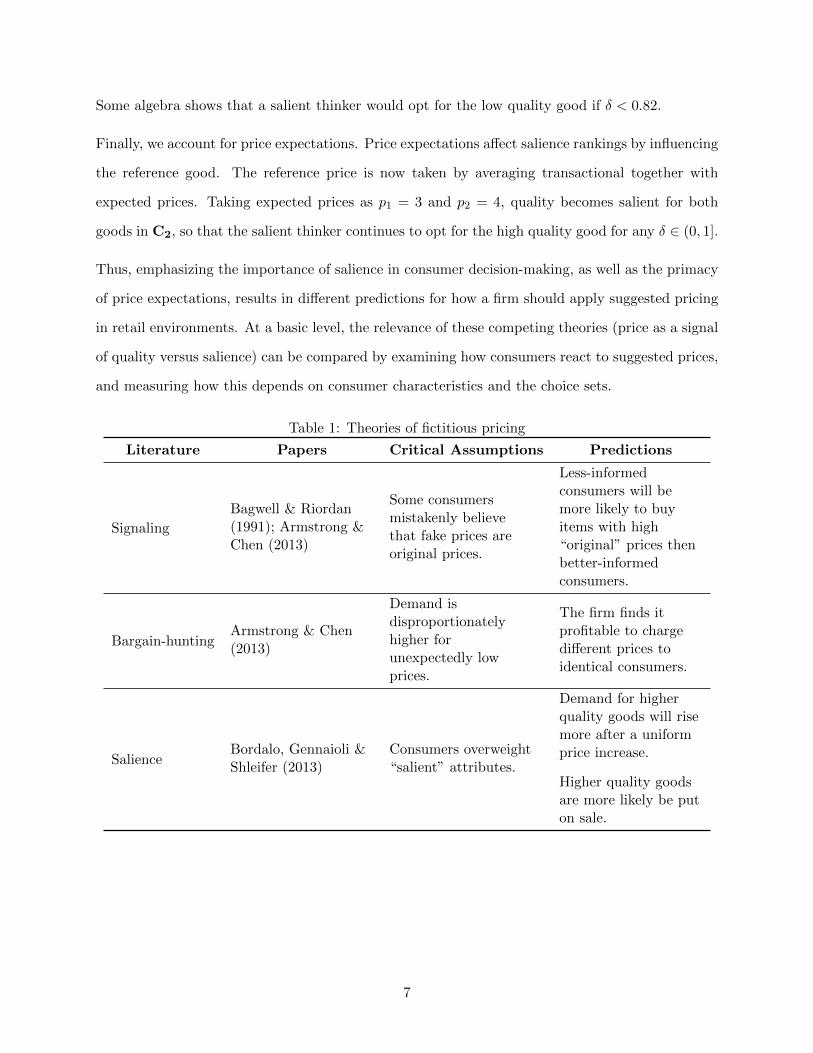
Table 1: Theories of fictitious pricing
Literature Papers Critical Assumptions Predictions
Signaling
Bagwell & Riordan(1991); Armstrong &Chen (2013)
Some consumersmistakenly believethat fake prices areoriginal prices.
Less-informedconsumers will bemore likely to buyitems with high“original” prices thenbetter-informedconsumers.
Bargain-huntingArmstrong & Chen(2013)
Demand isdisproportionatelyhigher forunexpectedly lowprices.
The firm finds itprofitable to chargedifferent prices toidentical consumers.
SalienceBordalo, Gennaioli &Shleifer (2013)
Consumers overweight“salient” attributes.
Demand for higherquality goods will risemore after a uniformprice increase.
Higher quality goodsare more likely be puton sale.
7
3 Data and industry background
Data is provided by a major fashion goods manufacturer and retailer in the United States. The
firm sells above 90% of its products by revenue through its own physical stores. The firm derives
the majority of its revenue from a single product type. All of the data and analysis in this chapter
concerns this single product category. The firm is the market leader in this category.
The firm operates two types of stores: regular and outlet. Regular stores are centrally located and
do not typically offer discounts on products. Outlet stores are typically located an hour away from
city centers and offer deep discounts (both actual and suggested). The firm offers two main types of
goods: original and factory. Original goods are first sold at full price in regular stores and then sold
at a discount in outlet stores. Factory goods are only sold in outlet stores. The firm implements
suggested pricing through its factory goods, which carry original prices that are never transacted.
The data consists of transaction-level records over a 5-year period. Each record has the original
price of each item and any applied discount. Also included are consumer observables, including
billing zip code, date of first purchase from the firm, and household ID.
Consumers. Repeat purchases by consumers are observable in the data. A total of 16,019,140
unique consumers are observed to make purchases within the sample. The proportion of purchases
that are made by return consumers is significant (see Figure 1). In the firm’s outlet channel, 24%
of purchases are made by return consumers. Of this group, 38% have made purchases in the regular
channel.
Prices. Table 2 describes the pricing differences between original and factory goods in outlet stores.
Original goods are more expensive than factory goods on average, both in terms of list prices and
transactional prices. However, there is much variation in these prices over time; and factory goods
occasionally carry higher prices than original goods (see Figure C).
Figure 2 graphs the average percent discount over time for original goods and factory goods in the
firm’s outlet channel. Recall that original goods are sold at full price in the regular channel, while
factory goods are sold exclusively in the outlet channel. The similar trend in discount increase over
time for these two product classes reflects the firm’s policy of trimming prices at even rates across
8
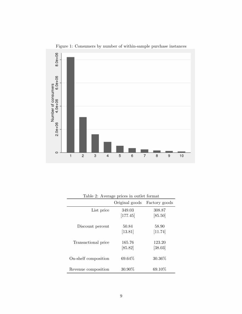
Figure 1: Consumers by number of within-sample purchase instances
Table 2: Average prices in outlet format
Original goods Factory goods
List price 349.03 308.87[177.45] [85.50]
Discount percent 50.84 58.90[13.81] [11.74]
Transactional price 165.76 123.20[85.82] [38.03]
On-shelf composition 69.64% 30.36%
Revenue composition 30.90% 69.10%
9
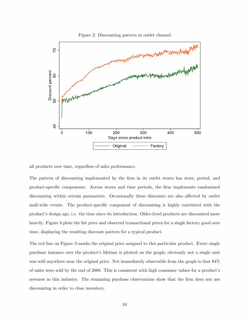
Figure 2: Discounting pattern in outlet channel
all products over time, regardless of sales performance.
The pattern of discounting implemented by the firm in its outlet stores has store, period, and
product-specific components. Across stores and time periods, the firm implements randomized
discounting within certain parameters. Occasionally these discounts are also affected by outlet
mall-wide events. The product-specific component of discounting is highly correlated with the
product’s design age, i.e. the time since its introduction. Older-lived products are discounted more
heavily. Figure 3 plots the list price and observed transactional prices for a single factory good over
time, displaying the resulting discount pattern for a typical product.
The red line on Figure 3 marks the original price assigned to this particular product. Every single
purchase instance over the product’s lifetime is plotted on the graph; obviously not a single unit
was sold anywhere near the original price. Not immediately observable from the graph is that 94%
of units were sold by the end of 2008. This is consistent with high consumer values for a product’s
newness in this industry. The remaining purchase observations show that the firm does not use
discounting in order to clear inventory.
10

Figure 3: Discounting pattern of a typical good
4 Demand model
In this section I present a simple discrete choice model of consumer purchase behavior and estimate
its parameters using data from a major fashion goods retailer. The main objective of estimation
is to verify that list prices affect purchase behavior keeping all other product attributes, including
the actual selling price, constant. I measure how this effect varies across consumer types. I proceed
to decompose consumer sensitivity to different components and ranges of discounting in order to
identify the margins in which suggested pricing is most effective. Finally, I test for the significance
of certain reference points that may influence the salience of discounting.
Let product j in store m and time t be defined by observable characteristics Xjt, unobserved quality
ξj , list price LPj , and transactional price pjmt. The utility of consumer i from purchasing product
j in market m is
uijmt = αpjmt +Xjtβ + γLPj + ξj + εijmt (2)
11
where α, β, and γ, are parameters to be estimated, and εijmt are idiosyncratic demand shocks.
Letting εijmt be iid Type-I extreme value, and inverting the resulting system of market share
equations (Berry 1994), we have that mean utilities can be written as
log(sjmt)− log(s0mt) = δjmt ≡ αpjmt +Xjtβ + γLPj + ξj
where sjmt are market shares and s0mt is the share of the outside good. A consumer is considered
to have chosen the outside good if she has visited a store but has not made a purchase. Availability
of foot traffic counts for each store-week enables direct observation of these outside shares.
Initial estimation of demand parameters is by OLS regression of mean utility levels on observables.
A market is defined as a store-week. The market size is taken to be the foot traffic recorded in each
store-week. Product characteristics Xjt include product age and categorical variables relating to
shape, color, material, and collection.2 Store and week fixed effects are also included. Descriptive
statistics for these variables in the estimation sample are reported in Table 3.3
Table 3: Sample descriptive statistics
Mean St. Dev. Count
Market size 9303.74 6442.74 Stores 124Market share 0.00074 0.00065 Weeks 27Price 120.80 32.84 Colors 350List price 337.73 63.37 Materials 29Age (days) 305.30 152.74 Silhouettes 20Factory 0.89 0.31 Collections 47
Estimates from the OLS regression are reported in column 1 of Table 4. Dummies for each categor-
ical variable, as well as for stores and weeks, are included in this and all succeeding regressions. As
anticipated, purchase probability is positively correlated with original price, and negatively with
the product’s design age. However, these estimates are likely biased and inconsistent owing to a
dependence of pjmt and LPj on ξj .
2A collection is a set of products that share the same general design features. Products are presented in shelvesaccording to their collection in the firm’s regular channel. In the firm’s outlet channel, products are grouped accordingto other physical characteristics.
3In this version, the estimation sample includes 27 weeks and 124 stores.
12
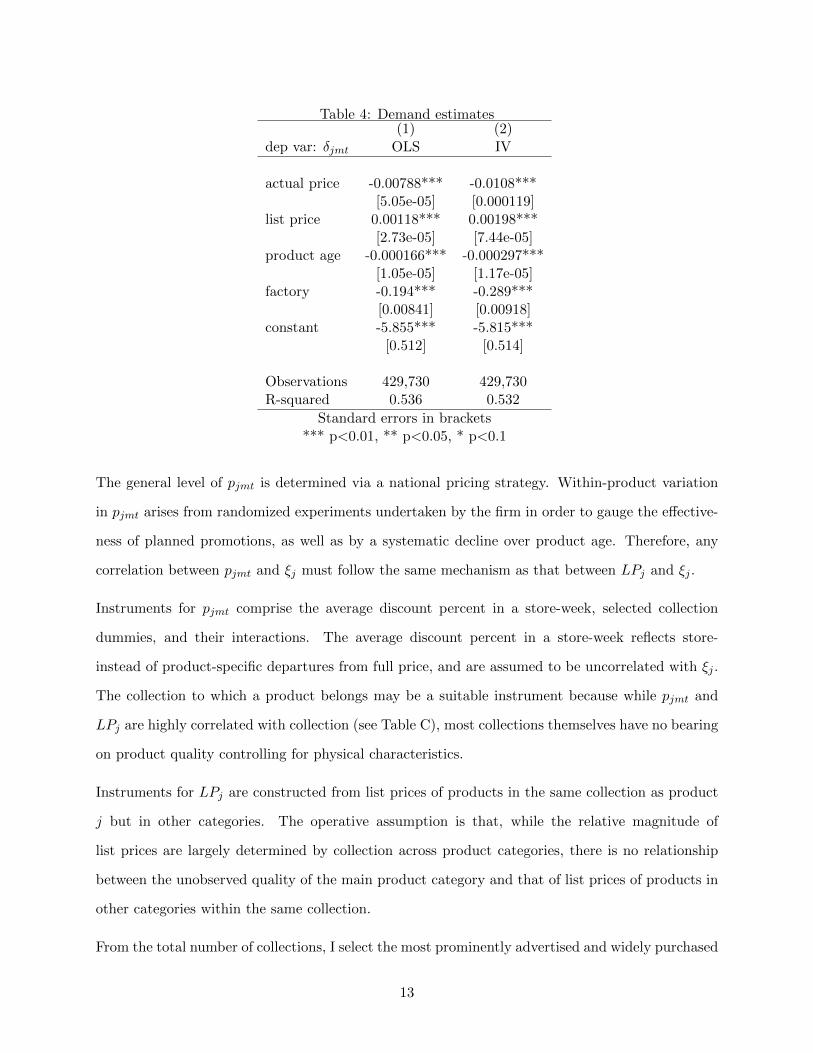
Table 4: Demand estimates(1) (2)
dep var: δjmt OLS IV
actual price -0.00788*** -0.0108***[5.05e-05] [0.000119]
list price 0.00118*** 0.00198***[2.73e-05] [7.44e-05]
product age -0.000166*** -0.000297***[1.05e-05] [1.17e-05]
factory -0.194*** -0.289***[0.00841] [0.00918]
constant -5.855*** -5.815***[0.512] [0.514]
Observations 429,730 429,730R-squared 0.536 0.532
Standard errors in brackets*** p<0.01, ** p<0.05, * p<0.1
The general level of pjmt is determined via a national pricing strategy. Within-product variation
in pjmt arises from randomized experiments undertaken by the firm in order to gauge the effective-
ness of planned promotions, as well as by a systematic decline over product age. Therefore, any
correlation between pjmt and ξj must follow the same mechanism as that between LPj and ξj .
Instruments for pjmt comprise the average discount percent in a store-week, selected collection
dummies, and their interactions. The average discount percent in a store-week reflects store-
instead of product-specific departures from full price, and are assumed to be uncorrelated with ξj .
The collection to which a product belongs may be a suitable instrument because while pjmt and
LPj are highly correlated with collection (see Table C), most collections themselves have no bearing
on product quality controlling for physical characteristics.
Instruments for LPj are constructed from list prices of products in the same collection as product
j but in other categories. The operative assumption is that, while the relative magnitude of
list prices are largely determined by collection across product categories, there is no relationship
between the unobserved quality of the main product category and that of list prices of products in
other categories within the same collection.
From the total number of collections, I select the most prominently advertised and widely purchased
13
collections as regressors in the second stage, and use the remaining collections as instruments in
the first stage. The reasoning is that, apart from the most popular among them, collections in the
outlet channel mainly serve as record-keeping devices for the firm, that while related to pricing,
are difficult for consumers to distinguish.
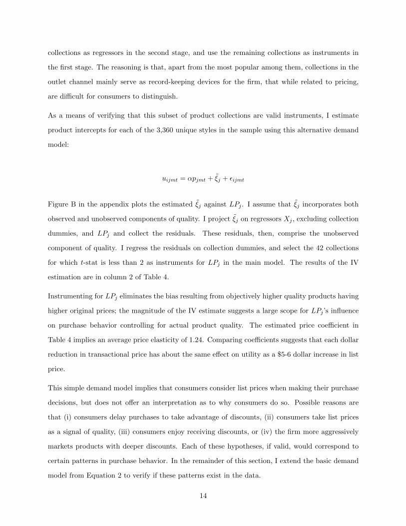
As a means of verifying that this subset of product collections are valid instruments, I estimate
product intercepts for each of the 3,360 unique styles in the sample using this alternative demand
model:
uijmt = αpjmt + ξj + εijmt
Figure B in the appendix plots the estimated ξj against LPj . I assume that ξj incorporates both
observed and unobserved components of quality. I project ξj on regressors Xj , excluding collection
dummies, and LPj and collect the residuals. These residuals, then, comprise the unobserved
component of quality. I regress the residuals on collection dummies, and select the 42 collections
for which t-stat is less than 2 as instruments for LPj in the main model. The results of the IV
estimation are in column 2 of Table 4.
Instrumenting for LPj eliminates the bias resulting from objectively higher quality products having
higher original prices; the magnitude of the IV estimate suggests a large scope for LPj ’s influence
on purchase behavior controlling for actual product quality. The estimated price coefficient in
Table 4 implies an average price elasticity of 1.24. Comparing coefficients suggests that each dollar
reduction in transactional price has about the same effect on utility as a $5-6 dollar increase in list
price.
This simple demand model implies that consumers consider list prices when making their purchase
decisions, but does not offer an interpretation as to why consumers do so. Possible reasons are
that (i) consumers delay purchases to take advantage of discounts, (ii) consumers take list prices
as a signal of quality, (iii) consumers enjoy receiving discounts, or (iv) the firm more aggressively
markets products with deeper discounts. Each of these hypotheses, if valid, would correspond to
certain patterns in purchase behavior. In the remainder of this section, I extend the basic demand
model from Equation 2 to verify if these patterns exist in the data.
14
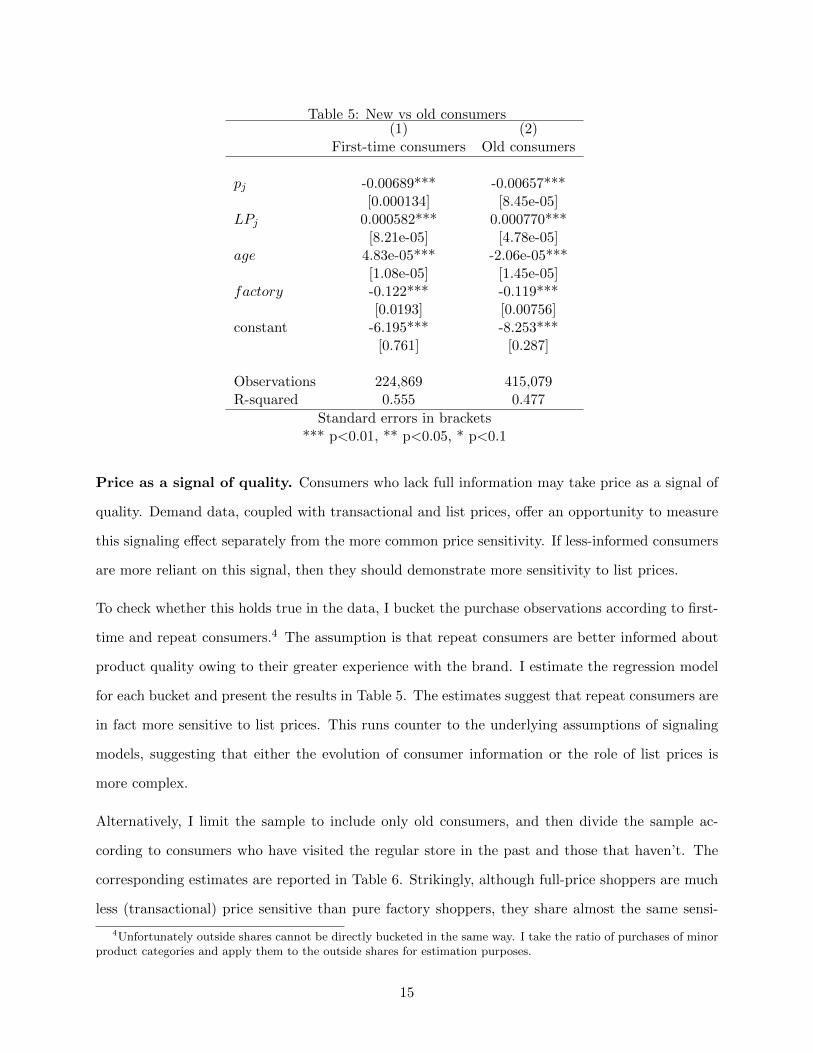
Table 5: New vs old consumers(1) (2)
First-time consumers Old consumers
pj -0.00689*** -0.00657***[0.000134] [8.45e-05]
LPj 0.000582*** 0.000770***[8.21e-05] [4.78e-05]
age 4.83e-05*** -2.06e-05***[1.08e-05] [1.45e-05]
factory -0.122*** -0.119***[0.0193] [0.00756]
constant -6.195*** -8.253***[0.761] [0.287]
Observations 224,869 415,079R-squared 0.555 0.477
Standard errors in brackets*** p<0.01, ** p<0.05, * p<0.1
Price as a signal of quality. Consumers who lack full information may take price as a signal of
quality. Demand data, coupled with transactional and list prices, offer an opportunity to measure
this signaling effect separately from the more common price sensitivity. If less-informed consumers
are more reliant on this signal, then they should demonstrate more sensitivity to list prices.
To check whether this holds true in the data, I bucket the purchase observations according to first-
time and repeat consumers.4 The assumption is that repeat consumers are better informed about
product quality owing to their greater experience with the brand. I estimate the regression model
for each bucket and present the results in Table 5. The estimates suggest that repeat consumers are
in fact more sensitive to list prices. This runs counter to the underlying assumptions of signaling
models, suggesting that either the evolution of consumer information or the role of list prices is
more complex.
Alternatively, I limit the sample to include only old consumers, and then divide the sample ac-
cording to consumers who have visited the regular store in the past and those that haven’t. The
corresponding estimates are reported in Table 6. Strikingly, although full-price shoppers are much
less (transactional) price sensitive than pure factory shoppers, they share almost the same sensi-
4Unfortunately outside shares cannot be directly bucketed in the same way. I take the ratio of purchases of minorproduct categories and apply them to the outside shares for estimation purposes.
15

Table 6: Pure factory vs full price shoppers(1) (2)
Pure factory Full-price
pj -0.00611*** -0.00393***[9.54e-05] [0.000107]
LPj 0.000564*** 0.000541***[5.92e-05] [6.14e-05]
age -2.84e-05*** -3.08e-05***[1.01e-05] [1.09e-05]
factory -0.118*** -0.122***[0.00764] [0.00824]
constant -7.926*** -7.708***[0.176] [0.237]
Observations 302,778 179,929R-squared 0.501 0.595
Standard errors in brackets*** p<0.01, ** p<0.05, * p<0.1
tivity to LPj .
An important distinction exists between original and factory goods in this market. Original goods
are those that were previously sold in the firm’s regular channel at their original prices. Factory
goods are those that were never sold in the regular channel, but are tagged with suggested prices.
Consumers in this market vary in their ability to distinguish original from factory goods. Presum-
ably consumers who have shopped in the regular channel in the past are more able to make this
distinction. Table 7 contains the estimated coefficient or the interaction of LPj and factory, an
indicator variable. As expected, list prices are a weaker signal of quality for factory goods.5
Table D limits the sample to repeat consumers and breaks consumers down according to their prior
purchase incidences and estimates the same interaction. Both groups discount list prices on factory
goods more than first-time consumers. Interestingly, both groups discount factory prices at about
40%, despite full-price consumers presumably being better able to distinguish factory goods from
original goods.
These estimates imply that while LPj may function as a signal of quality, it works in conjunction
5A Wald test of the null that the sum of the main and interaction coefficients, i.e. the list price sensitivity offactory goods, is zero is rejected at the 1% level.
16
Table 7: Interaction(1)
VARIABLES lhs
pj -0.0107***[0.000125]
LPj 0.00276***[9.58e-05]
LPj × factory -0.000308***[0.000107]
age -0.000268***[1.83e-05]
factory -0.188***[0.0437]
constant -6.283***[0.524]
Observations 429,730R-squared 0.534
Standard errors in brackets*** p<0.01, ** p<0.05, * p<0.1
Table 8: Consumer sensitivity to list prices(1) (2) (3) (4)
Shopper type Discount Discount Full-price Full-price
pj -0.00792*** -0.00793*** -0.00624*** -0.00635***[8.89e-05] [8.25e-05] [0.000115] [0.000121]
LPj 0.00173*** 0.00278*** 0.00158*** 0.00189***[4.33e-05] [9.67e-05] [6.06e-05] [0.000147]
LPj × factory -0.000992*** -0.000485***[9.34e-05] [0.000134]
constant -9.004*** -9.136*** -7.432 -7.727[0.622] [0.624] [0.483] [0.498]
Observations 185,387 185,387 92,739 92,739R-squared 0.559 0.559 0.622 0.622
Standard errors in brackets*** p<0.01, ** p<0.05, * p<0.1
17
with other effects. It is also likely that the signaling mechanism is more complex than what these
simple demand models can capture. In what follows I include various reference points to the
consumer’s utility function in an effort to parse these effects without adding complexity to the
model.
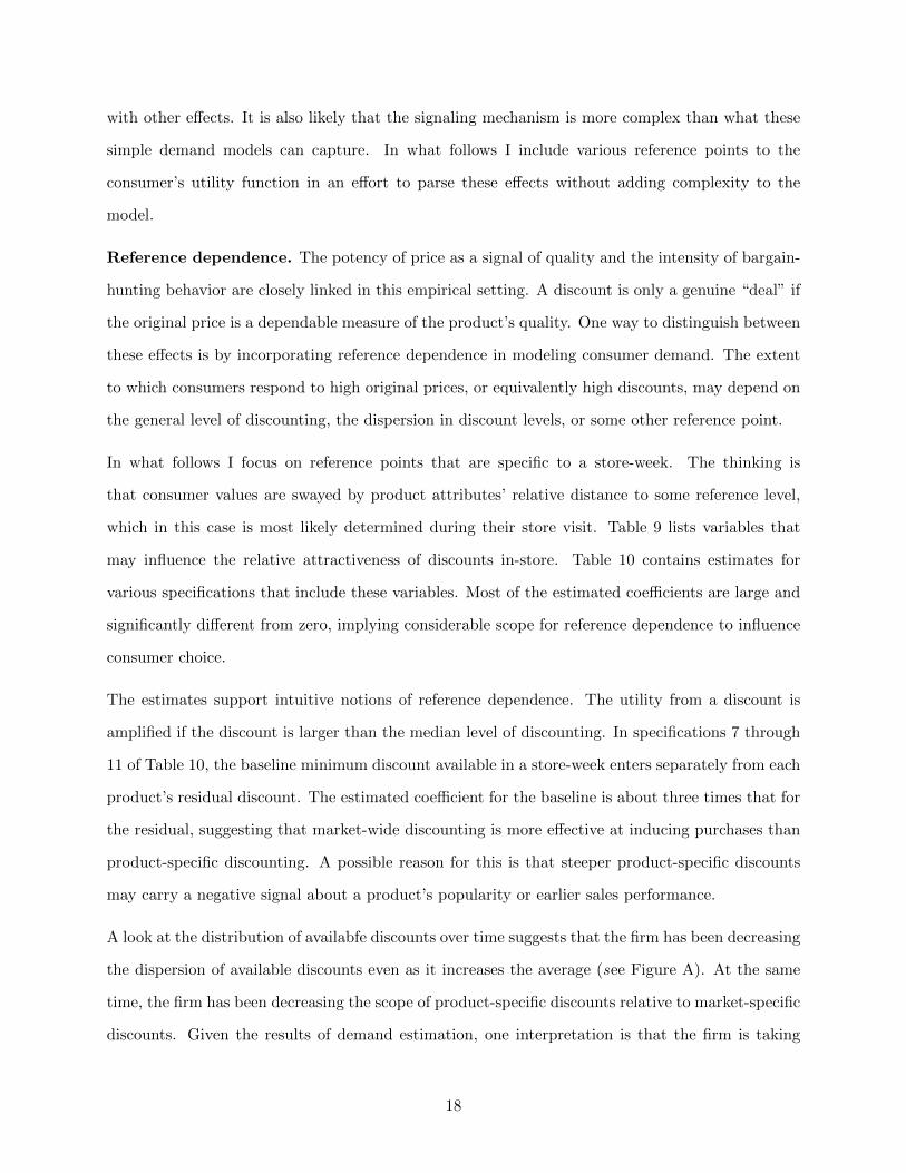
Reference dependence. The potency of price as a signal of quality and the intensity of bargain-
hunting behavior are closely linked in this empirical setting. A discount is only a genuine “deal” if
the original price is a dependable measure of the product’s quality. One way to distinguish between
these effects is by incorporating reference dependence in modeling consumer demand. The extent
to which consumers respond to high original prices, or equivalently high discounts, may depend on
the general level of discounting, the dispersion in discount levels, or some other reference point.
In what follows I focus on reference points that are specific to a store-week. The thinking is
that consumer values are swayed by product attributes’ relative distance to some reference level,
which in this case is most likely determined during their store visit. Table 9 lists variables that
may influence the relative attractiveness of discounts in-store. Table 10 contains estimates for
various specifications that include these variables. Most of the estimated coefficients are large and
significantly different from zero, implying considerable scope for reference dependence to influence
consumer choice.
The estimates support intuitive notions of reference dependence. The utility from a discount is
amplified if the discount is larger than the median level of discounting. In specifications 7 through
11 of Table 10, the baseline minimum discount available in a store-week enters separately from each
product’s residual discount. The estimated coefficient for the baseline is about three times that for
the residual, suggesting that market-wide discounting is more effective at inducing purchases than
product-specific discounting. A possible reason for this is that steeper product-specific discounts
may carry a negative signal about a product’s popularity or earlier sales performance.
A look at the distribution of availabfe discounts over time suggests that the firm has been decreasing
the dispersion of available discounts even as it increases the average (see Figure A). At the same
time, the firm has been decreasing the scope of product-specific discounts relative to market-specific
discounts. Given the results of demand estimation, one interpretation is that the firm is taking
18

Table 9: Description of variable labels in Table 10Model Regressor Definition
1 discount original price less transactional price
2 discount2 discount2
3 higher indicator for above-median discountdisc higher higher × discount
4 discz within-market z-score of discountdiscz disc discz × discount
5 posz positive z-scoresnegz negative z-scoresdisc pos discount × poszdisc neg discount × negz
6 avedisc average discount in marketsddisc st dev of discount in marketdisc ave discount × avediscdisc sd discount × sddisc
7 mindisc minimum discount in marketresid disc discount less mindisc
8 resid disc2 resid disc2
9 upper indicator for above-median resid discup resid resid disc × upper
10 residdiscz within-market z-score of resid discresiddiscz resid disc resid disc × residdiscz
11 rposz positive values of residdisczrnegz negative values of residdisczrdisc pos resid disc × rposzrdisc neg resid disc × rnegz
19

Tab
le10
:R
efer
ence
poi
nts
(1)
(2)
(3)
(4)
(5)
(6)
(7)
(8)
(9)
(10)
(11)
price
-0.00639***
-0.00638***
-0.00635***
-0.00638***
-0.00638***
-0.00635***
-0.00636***
-0.00636***
-0.00635***
-0.00636***
-0.00635***
[4.03e-0
5]
[4.03e-0
5]
[4.04e-0
5]
[4.04e-0
5]
[4.04e-0
5]
[4.04e-0
5]
[4.03e-0
5]
[4.03e-0
5]
[4.04e-0
5]
[4.03e-0
5]
[4.04e-0
5]
age
-6.67e-0
5***
-6.02e-0
5***
-6.25e-0
5***
-6.19e-0
5***
-7.01e-0
5***
-6.84e-0
5***
-6.40e-0
5***
-6.01e-0
5***
-5.95e-0
5***
-6.18e-0
5***
-6.53e-0
5***
[1.15e-0
5]
[1.15e-0
5]
[1.15e-0
5]
[1.15e-0
5]
[1.16e-0
5]
[1.15e-0
5]
[1.15e-0
5]
[1.15e-0
5]
[1.15e-0
5]
[1.15e-0
5]
[1.16e-0
5]
facto
ry-0
.210***
-0.205***
-0.217***
-0.206***
-0.218***
-0.213***
-0.210***
-0.207***
-0.212***
-0.208***
-0.217***
[0.0113]
[0.0113]
[0.0114]
[0.0114]
[0.0114]
[0.0113]
[0.0113]
[0.0113]
[0.0113]
[0.0113]
[0.0114]
discount
0.00101***
0.000306***
2.35e-0
50.000927***
0.00125***
-0.00288***
[2.93e-0
5]
[9.33e-0
5]
[5.95e-0
5]
[0.000107]
[0.000111]
[0.000318]
discount2
1.36e-0
6***
[1.70e-0
7]
higher
-0.285***
[0.0142]
dischigher
0.00137***
[6.70e-0
5]
discz
-0.0137**
[0.00578]
disczdisc
6.21e-0
5***
[1.11e-0
5]
discpos
-5.91e-0
5***
[1.67e-0
5]
discneg
0.000461***
[5.91e-0
5]
posz
0.0215***
[0.00759]
negz
-0.104***
[0.0111]
discave
2.16e-0
5***
[1.25e-0
6]
discsd
-1.52e-0
5***
[2.22e-0
6]
avedisc
-0.00283***
[0.000315]
sddisc
0.00302***
[0.000514]
min
disc
0.00299***
0.00291***
0.00284***
0.00257***
0.00268***
[8.91e-0
5]
[9.05e-0
5]
[9.16e-0
5]
[0.000128]
[0.000130]
resid
disc
0.000996***
0.000738***
0.000467***
0.000520***
0.000753***
[2.93e-0
5]
[6.32e-0
5]
[5.99e-0
5]
[0.000111]
[0.000114]
resid
disc2
7.71e-0
7***
[1.67e-0
7]
up
resid
0.000730***
[6.90e-0
5]
upper
-0.0826***
[0.00841]
residdiscz
0.0170***
[0.00555]
residdisczre
sid
disc
4.53e-0
5***
[1.11e-0
5]
rdiscpos
-6.75e-0
5***
[1.66e-0
5]
rdiscneg
0.000160**
[6.25e-0
5]
rposz
0.0451***
[0.00643]
rnegz
-0.0179***
[0.00690]
Constant
-7.023***
-6.903***
-6.809***
-6.983***
-7.093***
-6.550***
-7.237***
-7.196***
-7.173***
-7.125***
-7.200***
[0.741]
[0.741]
[0.741]
[0.742]
[0.742]
[0.745]
[0.741]
[0.741]
[0.741]
[0.741]
[0.741]
Obse
rvations
429,730
429,730
429,730
429,727
429,727
429,727
429,730
429,730
429,730
429,727
429,727
R-square
d0.543
0.543
0.544
0.543
0.543
0.544
0.544
0.544
0.544
0.544
0.544
Sta
ndard
errors
inbra
ckets
***
p<0.01,**
p<0.05,*
p<0.1
20
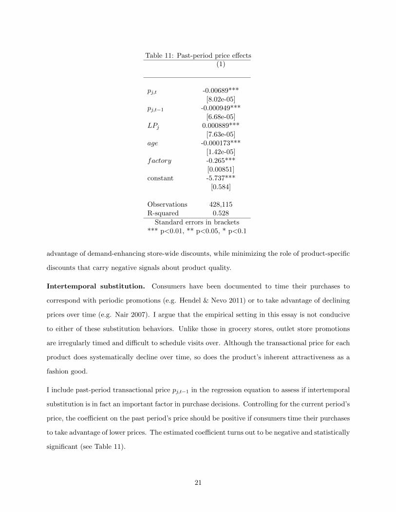
Table 11: Past-period price effects(1)
pj,t -0.00689***[8.02e-05]
pj,t−1 -0.000949***[6.68e-05]
LPj 0.000889***[7.63e-05]
age -0.000173***[1.42e-05]
factory -0.265***[0.00851]
constant -5.737***[0.584]
Observations 428,115R-squared 0.528
Standard errors in brackets*** p<0.01, ** p<0.05, * p<0.1
advantage of demand-enhancing store-wide discounts, while minimizing the role of product-specific
discounts that carry negative signals about product quality.
Intertemporal substitution. Consumers have been documented to time their purchases to
correspond with periodic promotions (e.g. Hendel & Nevo 2011) or to take advantage of declining
prices over time (e.g. Nair 2007). I argue that the empirical setting in this essay is not conducive
to either of these substitution behaviors. Unlike those in grocery stores, outlet store promotions
are irregularly timed and difficult to schedule visits over. Although the transactional price for each
product does systematically decline over time, so does the product’s inherent attractiveness as a
fashion good.
I include past-period transactional price pj,t−1 in the regression equation to assess if intertemporal
substitution is in fact an important factor in purchase decisions. Controlling for the current period’s
price, the coefficient on the past period’s price should be positive if consumers time their purchases
to take advantage of lower prices. The estimated coefficient turns out to be negative and statistically
significant (see Table 11).
21
5 Conclusion
Price comparisons, whether suggested or not, have become ubiquitous signals in retail settings. The
question of how these signals affect purchase behavior is relevant to firms, regulators, and perhaps
consumers themselves. Firms, in list prices, possess a potentially powerful driver of demand that
is virtually costless to produce and adjust. Regulators face the challenge of assessing whether
list prices inform or deceive, and ultimately whether they enhance or damage consumer welfare.
Consumers may be surprised to find out how list prices are determined, and the extent to which
their own decisions are reliant on them.
This chapter shows that list prices have significant effects on purchase decisions that may operate
through several channels. On average, consumers may be thought of as assigning a monetary
value to list prices at over 20 actual cents to a suggested dollar. This rate seems invariant to the
consumer’s depth of experience with a brand.
In addition, values for discounts depend on market-specific reference points. For instance, discount
sensitivity is much higher at levels above the average discount in a market. Consumers are also
more sensitive to discounts where the variance of discounting is higher. These suggest that optimal
price-setting by the firm should incorporate reference dependence in consumer behavior.
For future work, I plan on incorporating consumer heterogeneity in measuring the impact of sug-
gested pricing. Efforts at identifying the effect of heterogeneity in this chapter rely on strong
assumptions about how past shopping experience affects consumer information and behavior. Re-
laxing these assumptions by allowing list price effects to vary flexibly may be provide clues as to
which consumer segments are most swayed by list prices.
I also plan to study how consumer behavior provides incentives for the firm to pursue a strategy
of setting suggested prices. Since this form of price-setting is costless to the firm, there must be
countervailing forces that make setting ever-higher suggested original prices suboptimal. Identifying
these countervailing forces is necessary to make the firm’s suggested pricing optimization problem
well-defined.
The existing literature on price as a signal of quality views suggested list prices only as a means
22
of deceiving uninformed consumers. This literature relies on the strictly monotonic relationship of
quality and marginal cost as providing credibility to actual selling price as a signal of quality. In
the future, I plan on developing a model in which quality is generated through a stochastic process
indexed by marginal cost, and exploring the role that list prices can play in reducing asymmetric
information about quality between the firm and consumers. This is motivated by settings in which
quality can only imperfectly be set by firms, such as in fashion and design related industries.
References
[1] Armstrong, Mark, and Yongmin Chen. “Discount pricing.” Mimeo. (2012).
[2] Berry, Steven T. “Estimating discrete-choice models of product differentiation.” The RAND
Journal of Economics (1994): 242-262.
[3] Bagwell, Kyle, and Michael H. Riordan. “High and declining prices signal product quality.” The
American Economic Review (1991): 224-239.
[4] Bordalo, Pedro, Gennaioli, Nicola, and Andrei Shleifer. “Salience and consumer choice.” The
Journal of Political Economy (2013): 803-843.
[5] Dolan, Maura. “Kohl’s can be sued over sale ads, court says.” Los Angeles Times. May 22,
2013.
[6] Hastings, Justine, and Jesse M. Shapiro. Mental accounting and consumer choice: Evidence
from commodity price shocks. No. w18248. National Bureau of Economic Research, 2012.
[7] Hendel, Igal, and Aviv Nevo. Intertemporal price discrimination in storable goods markets. No.
w16988. National Bureau of Economic Research, 2011.
[8] Nair, Harikesh.“Intertemporal price discrimination with forward-looking consumers: Applica-
tion to the US market for console video-games.” Quantitative Marketing and Economics 5.3
(2007): 239-292.
[9] Pitofsky, Robert, Randal Shaheen, and Amy Mudge. “Pricing Laws Are No Bargain for Con-
sumers.” Antitrust 18 (2003): 62.
23

[10] Thaler, Richard. “Mental accounting and consumer choice.” Marketing Science 4.3 (1985):
199-214.
24

Appendix
Table A: Frequency of list prices
List price Percent of styles Average transacted price Discount Percent original styles
298 15.84 114.63 60.68 40.80398 10.87 149.30 61.21 45.65358 9.14 141.59 59.93 37.93348 6.54 123.45 63.82 61.45328 6.38 104.72 67.30 74.07198 5.67 96.00 50.52 9.72278 4.33 113.80 58.13 12.73498 4.02 190.59 61.08 17.65268 3.62 102.72 59.97 32.61598 3.23 249.80 57.55 9.76248 2.60 91.30 62.32 57.58258 2.52 91.38 61.35 6.25458 2.29 150.79 66.45 27.59428 2.29 149.41 64.37 72.41378 2.21 129.50 64.31 60.71
25

Figure A: Average discount percent in outlet stores
Table B: TrafficDependent variable: foot traffic (1) (2)
discount pctt 69.40*** 68.26***[1.770] [1.806]
discount pctt−1 -5.819***[1.800]
constant 5,486*** 6,943***[1,699] [2,396]
store fixed effects yes yesweek fixed effects yes yes
Observations 24,672 24,535R-squared 0.829 0.829
Standard errors in brackets*** p<0.01, ** p<0.05, * p<0.1
26
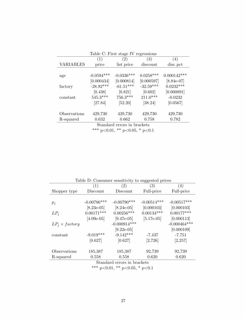
Table C: First stage IV regressions(1) (2) (3) (4)
VARIABLES price list price discount disc pct
age -0.0594*** -0.0336*** 0.0258*** 0.000142***[0.000434] [0.000814] [0.000597] [8.84e-07]
factory -28.92*** -61.51*** -32.59*** 0.0232***[0.438] [0.821] [0.602] [0.000891]
constant 545.3*** 756.3*** 211.0*** -0.0232[27.84] [52.20] [38.24] [0.0567]
Observations 429,730 429,730 429,730 429,730R-squared 0.632 0.662 0.758 0.782
Standard errors in brackets*** p<0.01, ** p<0.05, * p<0.1
Table D: Consumer sensitivity to suggested prices(1) (2) (3) (4)
Shopper type Discount Discount Full-price Full-price
pj -0.00786*** -0.00790*** -0.00514*** -0.00517***[8.23e-05] [8.24e-05] [0.000103] [0.000103]
LPj 0.00171*** 0.00256*** 0.00134*** 0.00177***[4.09e-05] [9.47e-05] [5.17e-05] [0.000113]
LPj × factory -0.000914*** -0.000464***[9.22e-05] [0.000109]
constant -9.019*** -9.142*** -7.437 -7.751[0.627] [0.627] [2,726] [2,257]
Observations 185,387 185,387 92,739 92,739R-squared 0.558 0.558 0.620 0.620
Standard errors in brackets*** p<0.01, ** p<0.05, * p<0.1
27
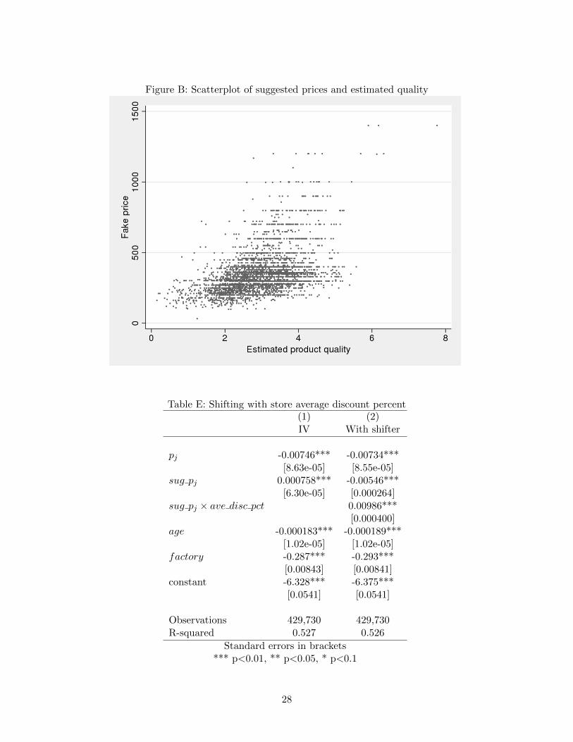
Figure B: Scatterplot of suggested prices and estimated quality
Table E: Shifting with store average discount percent(1) (2)IV With shifter
pj -0.00746*** -0.00734***[8.63e-05] [8.55e-05]
sug pj 0.000758*** -0.00546***[6.30e-05] [0.000264]
sug pj × ave disc pct 0.00986***[0.000400]
age -0.000183*** -0.000189***[1.02e-05] [1.02e-05]
factory -0.287*** -0.293***[0.00843] [0.00841]
constant -6.328*** -6.375***[0.0541] [0.0541]
Observations 429,730 429,730R-squared 0.527 0.526
Standard errors in brackets*** p<0.01, ** p<0.05, * p<0.1
28

Figure C: Prices over time
29