Embed Size (px)
Citation preview
Field and Laboratory Investigation of Asphalt Pavement
Permeability
by
Moustafa Awadalla
B.Sc. American University of Sharjah
A thesis submitted to the Faculty of Graduate and Postdoctoral
Affairs in partial fulfillment of the requirements for the degree of
Master of Applied Science
In
Civil Engineering
Ottawa-Carleton Institute of Civil and Environmental Engineering
Carleton University
Ottawa, Ontario
© 2015, Moustafa Awadalla
ii
Abstract
The long-term performance of road pavements is highly dependent upon the construction
quality of the newly paved sections. The current assessment method used to evaluate the
as-built quality of the newly finished roads utilizes relative density alone which may not
necessarily reflect the actual properties that are required in the finished pavement. This
research aims to perform comprehensive investigations concerning the hot mix asphalt
(HMA) pavement permeability as a potential quality indicator of newly constructed
roads. According to the conducted research, it is quite evident that considering the
permeability along with relative density in the design mix procedure should provide a
better indication and representation of the actual as-built physical condition of the newly
constructed HMA road pavements.

iii
Acknowledgements
Foremost, I would like to express all my gratitude to Allah for giving me the spiritual
support and strength to accomplish this dissertation successfully.
I would also love to express my deepest and sincere gratitude to each of my dear thesis
supervisors, Professor A. O. Abd El Halim and Professor Yasser Hassan, for providing
me with all necessary support and guidance throughout my studying period. Their
valuable feedback and constructive criticism to my thoughts were behind the success of
this research. I would like to extend my honest thanks and appreciation to the examining
committee, Professor John A. Goldak and Professor Shawn Kenny, for their comments
and feedback on my thesis study.
My deepest appreciation goes to my parents, Samir and Samiah, for supporting me
spiritually and financially through this journey. I cannot forget my dear siblings, Ahmed,
Hala, Sara, and Mohammed, for all their encouragement and for remembering me in their
prayers.
Special thanks go to my colleague Anandkumar Chelliah for providing me with all
assistance in collecting the field and laboratory data. Last but not least, I would love to
thank my dearest friend and brother, Mohammed Atef, for his support and sincere advice.
The financial support provided by the Ministry of Transportation of Ontario (MTO) is highly
appreciated and acknowledged.

iv
Table of Contents
Abstract .............................................................................................................................. ii
Acknowledgements .......................................................................................................... iii
Table of Contents ............................................................................................................. iv
List of Tables .................................................................................................................... vi
List of Figures ................................................................................................................. viii
List of Appendices ........................................................................................................... xii
Chapter 1: Introduction ............................................................................................................ 1
1.1 Background ................................................................................................................ 1
1.2 Problem Definition ..................................................................................................... 3
1.3 Objectives ................................................................................................................... 4
1.4 Scope of Research ...................................................................................................... 4
1.5 Thesis Organization ................................................................................................... 5
Chapter 2: Literature Review .................................................................................................. 6
2.1 Background ................................................................................................................ 6
2.2 Theoretical Background of Asphalt Pavement Permeability ..................................... 9
2.3 Factors Affecting Permeability ................................................................................ 10
2.4 Field Compaction Methods ...................................................................................... 13
2.5 Permeability Testing Techniques ............................................................................. 17
Chapter 3: Experimental Program ........................................................................................ 38
3.1 Data Collection......................................................................................................... 38
3.2 Equipment and Methods .......................................................................................... 45
3.3 Summary .................................................................................................................. 61
Chapter 4: Results of the Experimental Program ................................................................ 62

v
4.1 Field Investigations .................................................................................................. 62
4.2 Laboratory Investigations ......................................................................................... 79
4.3 Summary .................................................................................................................. 92
Chapter 5: Data Analysis ........................................................................................................ 94
5.1 Physical and Mechanical Properties of Asphalt Pavement ...................................... 94
5.2 Correlations between the Physical and Mechanical Properties .............................. 114
5.3 Relative Density-IDT Relationship ........................................................................ 120
5.4 Relative Density-Permeability Relationship .......................................................... 128
5.5 Permeability- IDT Relationship ............................................................................. 137
5.6 Summary ................................................................................................................ 146
Chapter 6: Conclusions and Recommendations ................................................................. 149
6.1 Summary ................................................................................................................ 149
6.2 Conclusions ............................................................................................................ 151
6.3 Recommendations for Future Studies .................................................................... 154
List of References .......................................................................................................... 156
Appendices ..................................................................................................................... 162

vi
List of Tables
Table 2.1: Pavement Compaction Requirements Based on Relative Density [MTO, 2002] ........... 8
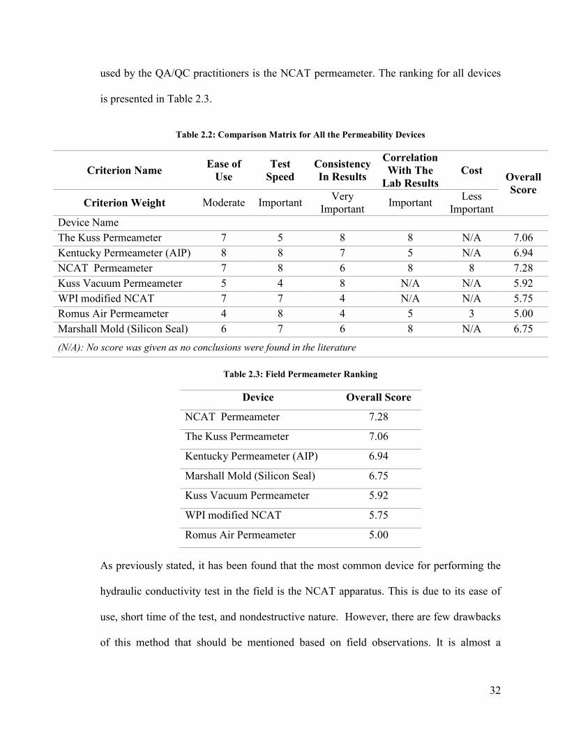
Table 2.2: Comparison Matrix for All the Permeability Devices .................................................. 32
Table 2.3: Field Permeameter Ranking.......................................................................................... 32
Table 3.1: The Research Experimental Plan .................................................................................. 41
Table 3.2: Superpave Volumetric Mix Design and Properties of the Three Available Mixes....... 57
Table 3.3: The Different Compaction Levels of SGC Specimens. ................................................ 59
Table 4.1: Summary of all Examined Projects from 2012 to 2014 ................................................ 63
Table 4.2: The Laboratory Results on SGC Specimens for the Four Considered Mixtures .......... 80
Table 5.1: Summary of the Relative Density Dataset .................................................................... 95
Table 5.2: Summary of the Three-Way ANOVA Test Hypotheses ............................................... 97
Table 5.3: Summary of the Three-Way ANOVA Results for Relative Density ............................ 98
Table 5.4: Summary of the IDT Dataset ........................................................................................ 99
Table 5.5: Summary of the Three-Way ANOVA Results for IDT .............................................. 101
Table 5.6: Summary of One-Way ANOVA Results for Effect of Compaction Method on IDT . 101
Table 5.7: Summary of the Field Permeability Dataset ............................................................... 102
Table 5.8: Summary of the Three-Way ANOVA Results for Field Permeability ....................... 105
Table 5.9: Summary of One-Way ANOVA Results for Effect Compaction Method on Field
Permeability ................................................................................................................................. 106
Table 5.10: Summary of the t-test Results for Effect of Age and Traffic on Field Permeability 107
Table 5.11: Summary of the Lab Permeability Dataset ............................................................... 107
Table 5.12: Summary of the Three-Way ANOVA Results for Lab Permeability ....................... 110
Table 5.13: Summary of the Dataset for Common Sites ............................................................. 111
Table 5.14: Summary of the Null and Alternative Hypotheses for Common Sites ..................... 114
Table 5.15: Summary of the One-way ANOVA Results for the common sites .......................... 114

vii
Table 5.16: Summary of the Correlation Coefficients and p-values for SGC Samples ............... 115
Table 5.17: Summary of the Correlation Coefficients and p-values for Conventional Method . 116
Table 5.18: Summary of the Correlation Coefficients and p-values for Advanced Method........ 117
Table 5.19: t-test Results for Examining the Difference between the Field and Lab Permeability
..................................................................................................................................................... 118
Table 5.20: Summary of Linear Regression Model between Field and Lab Permeability .......... 119
Table 5.21: Summary of the Regression Models between IDT and Relative Density (SCG
Specimens) ................................................................................................................................... 123
Table 5.22: Summary of the Regression Models between IDT and Relative Density (Field-
Recovered Cores) ......................................................................................................................... 128
Table 5.23: Summary of the Regression Models between Lab Permeability and Relative Density
(SCG Specimens) ......................................................................................................................... 131
Table 5.24: Summary of the Regression Models between Lab Permeability and Relative Density
(Field-Recovered Cores) .............................................................................................................. 133
Table 5.25: Summary of the Regression Models between Field Permeability and Relative Density
..................................................................................................................................................... 137
Table 5.26: Summary of the Regression Models between Lab Permeability and IDT (SCG
Specimens) ................................................................................................................................... 140
Table 5.27: Summary of the Regression Models between Lab Permeability and IDT (Field-
Recovered Cores) ......................................................................................................................... 144
Table 5.28: Summary of the Regression Models between Field Permeability and IDT .............. 146
Table 5.29: Summary of the Three-way ANOVA Results .......................................................... 147
viii
List of Figures
Figure 2.1: Darcy’s Apparatus [Lancellotta, 2008] ....................................................................... 10
Figure 2.2: Schematic of the Conventional Steel Drum Rolling [Abd El Halim and Mostafa,
2006] .............................................................................................................................................. 16
Figure 2.3: Schematic of the Advanced Rolling [Abd El Halim and Mostafa, 2006] ................... 17
Figure 2.4: NCAT Field Permeability Permeameter [Williams, 2006] ......................................... 18
Figure 2.5: Kuss Field Permeameter [Williams, 2006] ................................................................. 20
Figure 2.6: Typical Kuss Field Permeameter Data [Williams, 2006] ............................................ 22
Figure 2.7: Kentucky AIP [Cross and Bhusal, 2009] .................................................................... 23
Figure 2.8: Kuss Vacuum Permeameter [Williams, 2006] ............................................................ 25
Figure 2.9: WPI Modified NCAT Permeameter [Mallick, et al., 2003] ........................................ 26
Figure 2.10: Marshall Mold Permeameter Paraffin Seal [Cooley, 1999] ...................................... 27
Figure 2.11: Marshall Mold Permeameter Silicon Seal [Cooley, 1999] ........................................ 28
Figure 2.12: Romus Air Permeameter [Russell, et al., 2005; Retzer, 2008] .................................. 29
Figure 2.13: The Laboratory Permeability Device ........................................................................ 34
Figure 2.14: The CoreLok device [Instrotek®, 2011] ................................................................... 36
Figure 2.15: The Constant Head Permeameter [Maupin, 2000b] .................................................. 37
Figure 3.1: Experimental Program Plan ......................................................................................... 39
Figure 3.2: Location of Selected Sites in Ontario’s Eastern Region [d-maps, 2015] .................... 40
Figure 3.3: In-Situ Permeability Testing Layout ........................................................................... 44
Figure 3.4: The NCAT Field Permeameter .................................................................................... 46
Figure 3.5: In-situ Permeability Test at Highway 16 Project......................................................... 47
Figure 3.6: Karol-Warner Asphalt Permeameter ........................................................................... 49
Figure 3.7: Schematic the Lab Permeability Apparatus (Not to Scale) [Florida Test Method,
2012] .............................................................................................................................................. 50
ix
Figure 3.8: The Bulk Relative Density Testing Setup ................................................................... 52
Figure 3.9: The IDT Test on One of the Field-Recovered Cores ................................................... 54
Figure 3.10: The Laboratory Apparatus Required for SGC Specimen Preparation ....................... 56
Figure 3.11: Seize Analysis Gradation for the Considered Mixtures ............................................ 57
Figure 4.1: Field Permeability Result of Tomlinson In-house Field Trial (2012) ......................... 64
Figure 4.2: Field Permeability Result of Thousand Islands Parkway (2012) ................................ 64
Figure 4.3: Field Permeability Result of Highway 28 (2012) ........................................................ 65
Figure 4.4: Field Permeability Result of Tomlinson In-house Field Trial (2013) ......................... 66
Figure 4.5: Field Permeability Result of Highway 16 (2013) ........................................................ 66
Figure 4.6: Field Permeability Result of Highway 17 (2013) ........................................................ 67
Figure 4.7: Field Permeability Result of Highway 417 (2013) ...................................................... 67
Figure 4.8: Field Permeability Result of Highway 28 (2013) ........................................................ 68
Figure 4.9: Field Permeability Result of Thousand Islands Parkway (2013) ................................ 68
Figure 4.10: Field Permeability Result of Highway 15 before Microsurfacing (2013) ................. 69
Figure 4.11: Field Permeability Result of Highway 15 after Microsurfacing (2013) .................... 69
Figure 4.12: Field Permeability Result of Greenbelt Trial One (2014) ......................................... 70
Figure 4.13: Field Permeability Result of Highway 34 Bridge (2014) .......................................... 71
Figure 4.14: Summary of all 12 Investigated Projects Finished by the Conventional Method ..... 72
Figure 4.15: Field Permeability Result of Thousand Islands Parkway (2012) .............................. 73
Figure 4.16: Field Permeability Result of Tomlinson In-house Field Trial (2012) ....................... 74
Figure 4.17: Field Permeability Result of Highway 28 (2012) ...................................................... 74
Figure 4.18: Field Permeability Result of Thousand Islands Parkway (2013) .............................. 75
Figure 4.19: Field Permeability Result of Highway 28 (2013) ...................................................... 75
Figure 4.20: Field Permeability Result of Tomlinson In-house Field Trial (2013) ....................... 76
Figure 4.21: Field Permeability Result of Highway 34 Bridge (2014) .......................................... 77
Figure 4.22: Field Permeability Result of Greenbelt Trial One (2014) ......................................... 77
x
Figure 4.23: Summary of Projects Compacted by the Advanced Method ..................................... 78
Figure 4.24: The Average Relative Density Values corresponding to the Four Compaction Levels
....................................................................................................................................................... 81
Figure 4.25: The Average IDT Values corresponding to the Four Compaction Levels ................ 81
Figure 4.26: The Average Permeability Values corresponding to the Four Compaction Levels .. 82
Figure 4.27: Field Coring For the Inner Edge Location at Highway 417 Project .......................... 83
Figure 4.28: The Bulk Specific Gravity Results for year 2012 Projects ........................................ 85
Figure 4.29: The IDT Results for year 2012 Projects .................................................................... 85
Figure 4.30: The Bulk Specific Gravity Results for year 2013 Projects ........................................ 86
Figure 4.31: The Lab Permeability Results for year 2013 Projects ............................................... 87
Figure 4.32: The IDT Results for year 2013 Projects .................................................................... 87
Figure 4.33: The Laboratory Results of The in-house Field Trial at Greenbelt............................. 88
Figure 4.34: The Bulk Specific Gravity Results for year 2012 Projects ........................................ 89
Figure 4.35: The IDT Results for year 2012 Projects .................................................................... 90
Figure 4.36: The Bulk Specific Gravity Results for year 2014 Projects ........................................ 91
Figure 4.37: The Lab Permeability Results for year 2013 Projects ............................................... 91
Figure 4.38: The IDT Results for year 2014 Projects .................................................................... 92
Figure 5.1: Relative Density vs. Testing Locations (Conventional Method) ................................ 96
Figure 5.2: Relative Density vs. Testing Locations (Advanced Method) ...................................... 96
Figure 5.3: IDT vs. Testing Locations (Conventional Method)..................................................... 99
Figure 5.4: IDT vs. Testing Locations (Advanced Method) ........................................................ 100
Figure 5.5: Field Permeability vs. Testing Locations (Conventional Method) ............................ 103
Figure 5.6: Field Permeability vs. Testing Locations (Advanced Method) ................................. 104
Figure 5.7: Lab Permeability vs. Testing Locations (Conventional Method) .............................. 109
Figure 5.8: Lab Permeability vs. Testing Locations (Advanced Method) ................................... 109
xi
Figure 5.9: Comparison Between The Compaction Methods In Terms The Four Pavement
Properties ..................................................................................................................................... 112
Figure 5.10: Field and Laboratory Correlation ............................................................................ 119
Figure 5.11: The Relative Density-IDT Relationship for SGC Specimens ................................. 121
Figure 5.12: The General Trend of the Relative Density-IDT Relationship for SGC ................. 122
Figure 5.13: The Relative Density-IDT Relationship for Field Cores ......................................... 124
Figure 5.14: The Relative Density-IDT Relationship Categorized by Compaction Method ....... 125
Figure 5.15: The Relative Density-IDT Relationship for Field Cores (Conventional Method) .. 126
Figure 5.16: The Relative Density- IDT Relationship for Field Cores (Advanced Method) ....... 127
Figure 5.17: The Relative Density-Permeability Relationship for SGC Specimens.................... 129
Figure 5.18: The General Trend of the Relative Density-Permeability Relationship for SGC ... 130
Figure 5.19: The Relative Density-Permeability Relationship for Field Cores ........................... 132
Figure 5.21: The Correlation between Relative Density and Field Permeability ........................ 134
Figure 5.21: Field Permeability-Density Relationship Categorized by Compaction Method ..... 135
Figure 5.22: The Relative Density-Permeability Trend for Field Cores and Field Measurements
..................................................................................................................................................... 136
Figure 5.23: The Permeability- IDT Relationship for SGC Specimens ....................................... 138
Figure 5.24: The General Trend of the Strength-Permeability Relationship for SGC ................. 139
Figure 5.25: The Permeability- IDT Relationship for All Data Points ........................................ 141
Figure 5.26: The Permeability- IDT Relationship based on Compaction Method ...................... 142
Figure 5.27: The Permeability- IDT Relationship for Field Cores (Conventional Method) ........ 142
Figure 5.28: The Permeability- IDT Relationship for Field Cores (Advanced Method) ............. 143
Figure 5.29: The Correlation between IDT and Field Permeability ............................................ 145
xii
List of Appendices
Appendix A: ANOVA and t-test Results……………………………………………… 162
A.1 Relative Density………...……………………………………………….162
A.2 IDT…………………………………………………………...………….162
A.3 Field Permeability…….……………………………………...………….163
A.4 Lab Permeability…….….…….……………………………...………….165
A.5 Lab vs. Field Permeability……………………………………………....166
A.6 Comparison between the two compaction methods………………….......168
Appendix B: Regression Analysis……..……………………………………………… 169
B.1 Relative Density………...……………………………………………….169
B.2 Relative Density-IDT………...………………………………………….169
B.3 Relative Density-Permeability……….....……………………………….171
B.4 IDT-Permeability……………………………………………………......174
1
CHAPTER 1: INTRODUCTION
1.1 Background
The Canadian roadway system constitutes a considerable part of the total infrastructure
network. There are nearly one million kilometers of both paved and unpaved roads in
Canada, where Ontario alone has approximately 200,000 kilometers [Government of
Canada, 2012; OHMPA Asphalt Fact Sheet, 2012]. The Canadian economy,
environment, and public safety depend highly on how we maintain and monitor such a
crucial asset. The design and construction of road pavements consider various factors
including, but not limited to, pavement performance, traffic, environment, drainage, and
so forth. In general, the newly paved roads are expected to perform for a particular period
of time under various traffic loads and environmental conditions. However, it is common
to observe failure in these roads after short duration [Rollings and Rollings, 1991]. A
general dilemma faced by transportation jurisdictions is that fund dedicated for road
rehabilitation and maintenance is inadequate for every deteriorated section. Therefore, it
is vital to ensure that the newly built roads are properly designed, constructed, and met
the quality assurance/control (QA/QC) specifications. This should in turn maximize the
anticipated road service life as well as minimizing the overall rehabilitation cost and
maintenance.
Pavement structure is classified in terms of structural characteristics into two main types,
flexible and rigid pavement. On one hand, the flexible pavement is made of an asphalt (or
bituminous) layer followed down by base, subbase, and subgrade layer. On the other
hand, the rigid pavement has Portland cement concrete (PCC) surface course over the
subbase and subgrade layers [Garber and Hoel, 2014]. The most common type of flexible
2
pavements is the hot mix asphalt (HMA) which can be classified into three main
categories; the dense-graded mix, stone matrix asphalt or stone mastic asphalt (SMA),
and open-graded [Pavement Interactive, 2010]. The dense-graded mixes, which will be
considered in this study, are usually designed under a primary assumption of being
relatively impermeable to water and air.
The construction of road pavements incorporates several activities including mix
preparation, transportation, placement, and finally compaction. All the aforementioned
activities have crucial impacts on the overall long-term performance of road pavements.
Among these activities, compaction is the most influential factor governing the long-term
performance and durability of the newly constructed road sections [Geller, 1984]. In
other words, inadequate compaction efforts are expected to lead to poor pavement
performance even if all other essential variables (e.g. mixture design and favorable
environmental conditions) were met and achieved. Compaction can be defined as the
process by which the volume of air in an HMA mixture is reduced by using external
forces [Roberts, et al., 1996]. This reduction in air voids results in increasing the achieved
density to fall within an acceptable range set by transportation authorities. Evaluation of
compaction quality varies from one road jurisdiction to another depending on the
followed test method and its acceptance criteria. In general, the compaction quality can
be quantified by two common techniques [Pavement Interactive, 2009]. The first one
entails extracting some samples from the paved roadbed; these samples are termed field-
recovered cores. These cores are then shipped to a materials testing laboratory for density
determination. The other approach suggests measuring the in-place density using a
nuclear gauge, which is an automated device that sends gamma radiation through
3
pavement structure to estimate its density. It is worth mentioning that the second
approach is nondestructive, easier, and faster, than the first approach. However, it lacks
accuracy and consistency compared to the first approach [Williams, 2006].
1.2 Problem Definition
The current practice followed by road jurisdictions, specifically the Ministry of
Transportation Ontario (MTO), considers only one pavement property, which is the
relative density, to accept or reject the as-built condition of the newly paved roads [MTO,
2004]. The primary assumption of relaying on relative density as an indicator is that road
sections with acceptable relative density are more durable and will have better long-term
performance. In the as-built condition, acceptable levels of relative density may not be
sufficient to represent other important physical properties related to moisture and water
infiltration rates. In fact, various pavement failure modes including moisture-induced
damage, thermal and fatigue cracking, and potholes were observed at road pavements that
were considered accepted according to the current quality control specifications.
Consequently, it is not very rational to depend solely on one pavement property to
evaluate the newly built HMA road pavements. Alternatively, considering other
pavement characteristics could be beneficial in evaluating these new constructed roads
and should provide QA/QC engineers with sound understanding of the expected
pavement performance in short and long terms. There is no reliable method currently
used and adopted by road authorities to quantify the degree or quality of field compaction
based on laboratory procedure. There is a need to address the issue of using other
pavement properties when assessing the as-built pavement condition in order to ensure
attaining the highest possible quality. This new quality indicator(s) should be reliable and
4
representative of the actual as-built condition of newly paved roads. In addition, this
indicator should be measurable at both environments; the field and laboratory.
1.3 Objectives
The main set of objectives of this thesis is broken into three main goals. First and most
importantly, this research aims to study HMA asphalt pavement permeability, as an
important physical pavement characteristic related more to moisture-induced damages,
and compare/relate it to the relative density, the currently adopted quality indicator of
newly constructed HMA roads. Additionally, this dissertation is intended to perform
extensive field and laboratory investigations in an attempt to explore the possible
correlations between important physical (permeability and relative density) and
mechanical characteristics of HMA. The study also tries to examine the effect of different
factors including testing location, project level, and compaction method on the overall
performance of HMA roads in terms of particular physical and mechanical properties.
1.4 Scope of Research
The scope of this research is limited and oriented in certain directions to achieve the
stated objectives. Firstly, the study considers only HMA road pavements that are newly
constructed and other one year in-service roads. These newly paved sections serve the
needs of this research by evaluating only the as-built conditions and the short-term
performance. Secondly, the research investigates only one type of dense-graded HMA
asphalt pavement in terms of the aggregate size, which is 12.5mm as it is one of the most
commonly used mix type in Ontario. As well, the field data were collected at sites located
in Eastern Ontario to minimize the traveling distance needed for field investigations.
From laboratory perspective, the study is also limited to four loose asphalt mixtures of
5
the same aggregate size, 12.5 mm, provided by the MTO to ensure that these mixtures are
the same mixtures studied in the field.
1.5 Thesis Organization
This dissertation consists of six chapters. Chapter one introduces the conducted research
as well as stating the objectives and research scope. Chapter two describes the topic of
HMA permeability in addition to extensively reviewing the most current practices and
methods used to measure the HMA permeability. Chapter three describes the adopted
field and laboratory experimental program. Chapter four presents the results obtained by
performing the field and laboratory investigations. Chapter five shows the conducted
analysis along with discussing of obtained results. Chapter six summarizes the findings,
conclusions, and recommendations for future research.
6
CHAPTER 2: LITERATURE REVIEW
2.1 Background
The Superior Performing Asphalt Pavements (SuperPave) system is initiated in late 80s
by the Strategic Highway Research Program (SHRP) to provide the engineers,
technicians and highway jurisdictions with a robust philosophy of designing hot-mix
asphalt (HMA) pavement. One of the fundamental objectives of such design is to deliver
road pavements of high quality, maximum durability, and long term performance with
minimum distress issues under different environmental challenges over the pavement
lifespan [Pavement Interactive, 2009]. However, it is common to observe various
pavement failures that could be attributed to several causes such as the poor mixture
design, improper compaction effort, repeated traffic loads, and environmental effects
[Neal, 2014]. One of the most serious distresses leading to asphalt pavement failures is
the phenomenon known as the moisture induced damage, which is a distress that occurs
due to the presence of water within the pavement system and results in destroying the
bond within the asphalt mix [Howson, et al., 2009; Caro, et al., 2010].
The existence of trapped water within the pavement structures has led to negative
consequences by shortening the designed road service life or increasing the pavement
maintenance and rehabilitation costs. Road pavements that have been poorly designed,
compacted and/or constructed have higher chances of experiencing moisture related
damage which adversely affects the asphalt strength and durability. The possible results
of distress problems are moisture-induced cohesive and adhesive damage, fatigue
cracking, freeze-thaw failure and/or permanent deformation [Umiliaco and Benedetto,
2013]. These concerns have been well investigated by numerous researchers to quantify
7
the adverse effects of different distress problems [Chen, et al., 2004; Pang, 2012; Yong-
Rak, et al., 2004]. The pavement structure can also experience raveling, stripping,
potholing, and rutting.
The QA/QC are crucial tools for all highway jurisdictions and contractors in order to
ensure that the delivered asphalt pavements meet the end-result specifications. While the
current QA/QC practice in the province of Ontario resulted in improving the overall
performance of the Ontario roads, the in-service highway sections are still suffering from
distress problems after a relatively short period of time. This means that the as-built
pavement conditions were overestimated according to the conventional QA/QC methods
for HMA.
Subsequently, there is a need to establish an alternative approach that can objectively
assess the as-built pavement conditions and thus ensures that it will meet its projected
design life. According to the “Ontario Provincial Standards for Roads & Public Works
Archives: Construction Specification for Hot Mix Asphalt”, the pavement compaction
effort is measured by the maximum relative density of pavement structure [MTO, 2002].
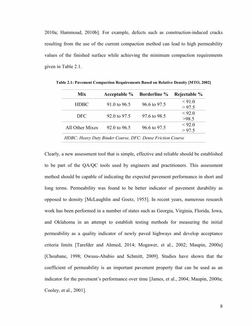
Table 2.1 shows the accepted and rejected densities in order to evaluate the pavement
compaction end results. Relying on the density alone in assessing the pavement quality
could be a misleading practice. Several researchers showed that meeting minimum
measured densities of finished asphalt pavement projects is not enough as a criterion to
guarantee meeting the design service life. Meeting relative densities or specified
compaction values of newly constructed asphalt mixes may not reflect the actual defects
that exist in the finished pavement [Mostafa, 2005; Abd El Halim and Mostafa, 2006;
Abd El Halim, et al., 2009; Brown, et al., 2004; Abd El Halim, et al., 2012; Hammoud,
8
2010a; Hammoud, 2010b]. For example, defects such as construction-induced cracks
resulting from the use of the current compaction method can lead to high permeability
values of the finished surface while achieving the minimum compaction requirements
given in Table 2.1.
Table 2.1: Pavement Compaction Requirements Based on Relative Density [MTO, 2002]
Mix Acceptable % Borderline % Rejectable %
HDBC 91.0 to 96.5 96.6 to 97.5 < 91.0
> 97.5
DFC 92.0 to 97.5 97.6 to 98.5 < 92.0
>98.5
All Other Mixes 92.0 to 96.5 96.6 to 97.5 < 92.0
> 97.5
HDBC: Heavy Duty Binder Course, DFC: Dense Friction Course
Clearly, a new assessment tool that is simple, effective and reliable should be established
to be part of the QA/QC tools used by engineers and practitioners. This assessment
method should be capable of indicating the expected pavement performance in short and
long terms. Permeability was found to be better indicator of pavement durability as
opposed to density [McLaughlin and Goetz, 1955]. In recent years, numerous research
work has been performed in a number of states such as Georgia, Virginia, Florida, Iowa,
and Oklahoma in an attempt to establish testing methods for measuring the initial
permeability as a quality indicator of newly paved highways and develop acceptance
criteria limits [Tarefder and Ahmed, 2014; Mogawer, et al., 2002; Maupin, 2000a]
[Choubane, 1998; Owusu-Ababio and Schmitt, 2009]. Studies have shown that the
coefficient of permeability is an important pavement property that can be used as an
indicator for the pavement’s performance over time [James, et al., 2004; Maupin, 2000a;
Cooley, et al., 2001].
9
2.2 Theoretical Background of Asphalt Pavement Permeability
The permeability (hydraulic conductivity) is the property that describes how water flows
through particular porous medium. Usually, the permeability is represented by the
coefficient of permeability (k) which is the constant of proportionality of the relationship
between the flow velocity and hydraulic gradient between two points in a particular
porous medium [Garber and Hoel, 2014]. The permeability of any porous medium can be
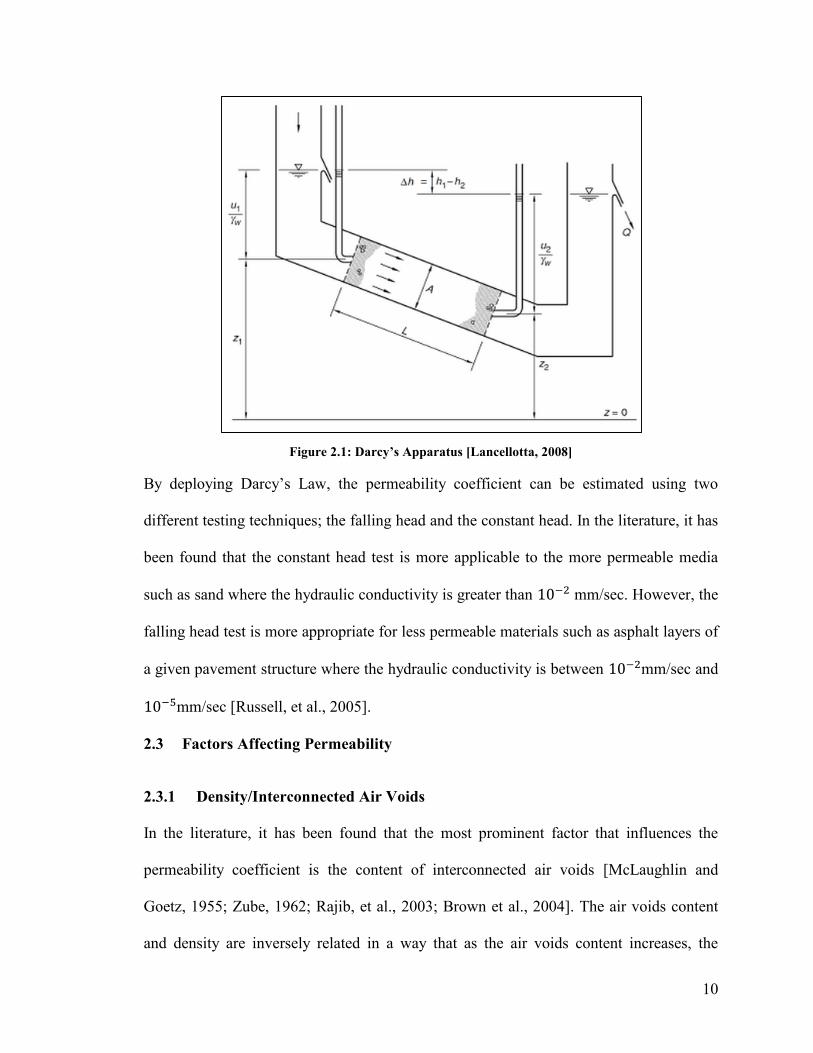
explained by the early work done by the French engineer Henry Darcy in 1856. Darcy’s
Law explains the term hydraulic conductivity in an experimental framework as shown in
Figure 2.1. Darcy’s law was an attempt to develop a water purification system using the
sand as the medium [Darcy, 1856]. Darcy’s Law statement is that the discharge velocity
of the fluid is directly proportional to the hydraulic gradient. Equation 2.1 represents
Darcy’s Law as follows:
𝑄 = 𝐾(∆ℎ
𝐿)𝐴 Equation 2.1
where:
K = proportional factor called hydraulic conductivity or permeability coefficient,
Q = rate of flow (volume of water per unit time),
A = cross-sectional area perpendicular to the flow direction,
∆h = change in the hydraulic head, and
L = length of flow.
10
Figure 2.1: Darcy’s Apparatus [Lancellotta, 2008]
By deploying Darcy’s Law, the permeability coefficient can be estimated using two
different testing techniques; the falling head and the constant head. In the literature, it has
been found that the constant head test is more applicable to the more permeable media
such as sand where the hydraulic conductivity is greater than 10−2 mm/sec. However, the
falling head test is more appropriate for less permeable materials such as asphalt layers of
a given pavement structure where the hydraulic conductivity is between 10−2mm/sec and
10−5mm/sec [Russell, et al., 2005].
2.3 Factors Affecting Permeability
2.3.1 Density/Interconnected Air Voids
In the literature, it has been found that the most prominent factor that influences the
permeability coefficient is the content of interconnected air voids [McLaughlin and
Goetz, 1955; Zube, 1962; Rajib, et al., 2003; Brown et al., 2004]. The air voids content
and density are inversely related in a way that as the air voids content increases, the
11
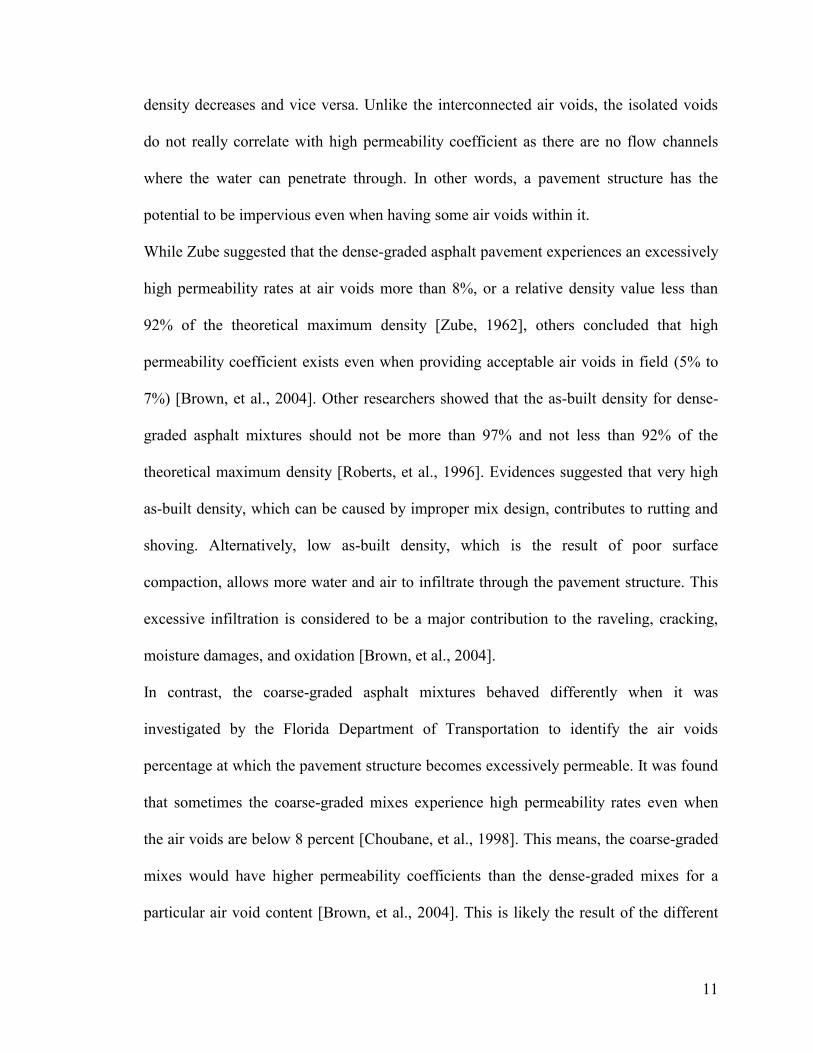
density decreases and vice versa. Unlike the interconnected air voids, the isolated voids
do not really correlate with high permeability coefficient as there are no flow channels
where the water can penetrate through. In other words, a pavement structure has the
potential to be impervious even when having some air voids within it.
While Zube suggested that the dense-graded asphalt pavement experiences an excessively
high permeability rates at air voids more than 8%, or a relative density value less than
92% of the theoretical maximum density [Zube, 1962], others concluded that high
permeability coefficient exists even when providing acceptable air voids in field (5% to
7%) [Brown, et al., 2004]. Other researchers showed that the as-built density for dense-
graded asphalt mixtures should not be more than 97% and not less than 92% of the
theoretical maximum density [Roberts, et al., 1996]. Evidences suggested that very high
as-built density, which can be caused by improper mix design, contributes to rutting and
shoving. Alternatively, low as-built density, which is the result of poor surface
compaction, allows more water and air to infiltrate through the pavement structure. This
excessive infiltration is considered to be a major contribution to the raveling, cracking,
moisture damages, and oxidation [Brown, et al., 2004].
In contrast, the coarse-graded asphalt mixtures behaved differently when it was
investigated by the Florida Department of Transportation to identify the air voids
percentage at which the pavement structure becomes excessively permeable. It was found
that sometimes the coarse-graded mixes experience high permeability rates even when
the air voids are below 8 percent [Choubane, et al., 1998]. This means, the coarse-graded
mixes would have higher permeability coefficients than the dense-graded mixes for a
particular air void content [Brown, et al., 2004]. This is likely the result of the different
12
contents of interconnected air voids in both types of mixes where coarse-graded mixes
will likely have more interconnected air voids than dense-graded mixes.
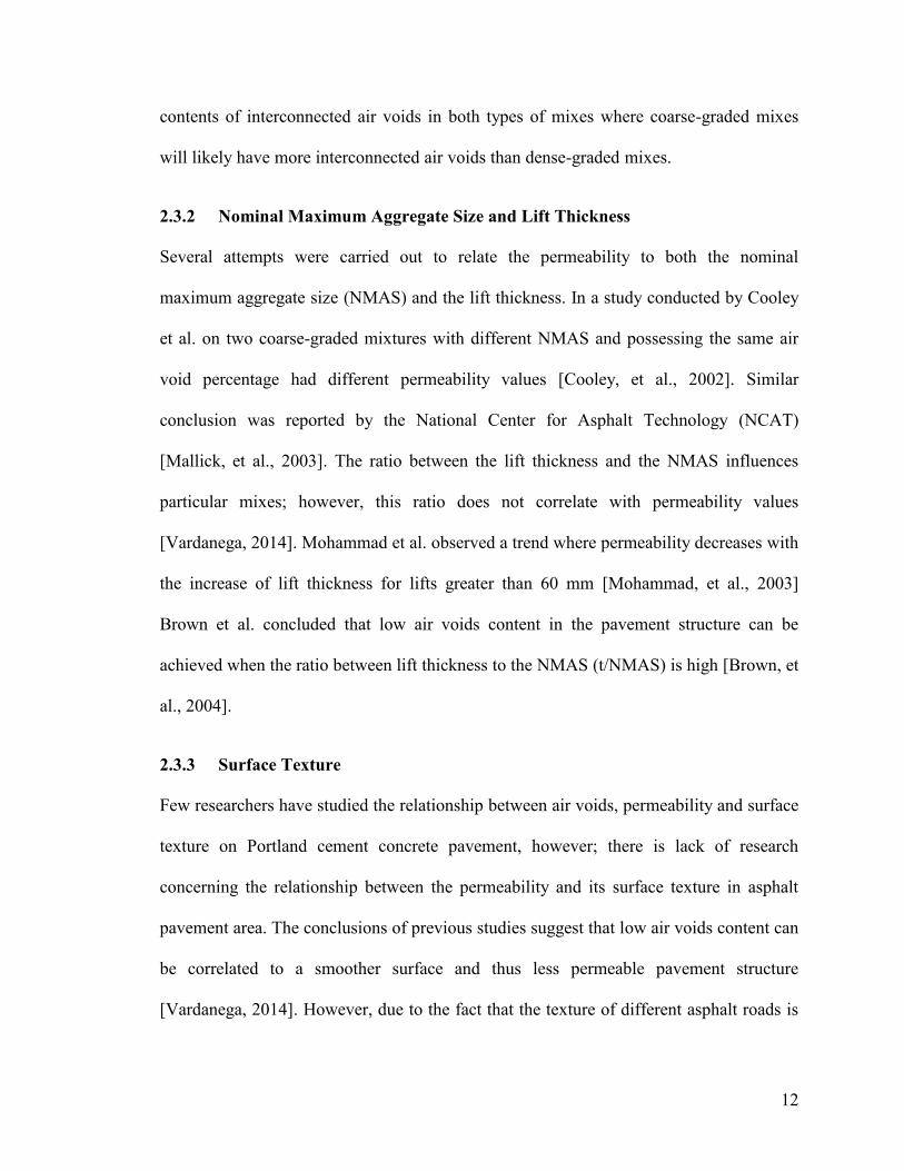
2.3.2 Nominal Maximum Aggregate Size and Lift Thickness
Several attempts were carried out to relate the permeability to both the nominal
maximum aggregate size (NMAS) and the lift thickness. In a study conducted by Cooley
et al. on two coarse-graded mixtures with different NMAS and possessing the same air
void percentage had different permeability values [Cooley, et al., 2002]. Similar
conclusion was reported by the National Center for Asphalt Technology (NCAT)
[Mallick, et al., 2003]. The ratio between the lift thickness and the NMAS influences
particular mixes; however, this ratio does not correlate with permeability values
[Vardanega, 2014]. Mohammad et al. observed a trend where permeability decreases with
the increase of lift thickness for lifts greater than 60 mm [Mohammad, et al., 2003]
Brown et al. concluded that low air voids content in the pavement structure can be
achieved when the ratio between lift thickness to the NMAS (t/NMAS) is high [Brown, et
al., 2004].
2.3.3 Surface Texture
Few researchers have studied the relationship between air voids, permeability and surface
texture on Portland cement concrete pavement, however; there is lack of research
concerning the relationship between the permeability and its surface texture in asphalt
pavement area. The conclusions of previous studies suggest that low air voids content can
be correlated to a smoother surface and thus less permeable pavement structure
[Vardanega, 2014]. However, due to the fact that the texture of different asphalt roads is
13
currently achieved using the same compaction technology, a scientific assessment of this
factor is not currently possible.
2.4 Field Compaction Methods
In the literature, compaction is defined as the process by which the volume of air in an
HMA mixture is reduced by using external forces to reorient the constituent aggregate
particles into a more closely spaced arrangement [Roberts, et al., 1996]. Reducing the air
voids will in turn result in increasing the HMA density level. This dissertation studied
two field compaction equipment that are designed and operated based on different
principles. In this research, the term “conventional” refers to the current compaction
methods, while the term “advanced” refers to a recent developed compaction technology.
2.4.1 Conventional Compaction Methods
The currently common practice followed by HMA community to compact new roadways
is carried out using three basic pieces of self-propelled equipment of different functions.
These equipment are, the steel static wheeled roller, pneumatic tire roller, and vibratory
static wheeled roller. First, a paver screed places the HMA over the road base course.
Then, the steel wheeled roller passes over the placed mix to apply the required
compressive forces and achieve the desired relative density. In general, the steel roller
(static or vibratory) has a roller diameter that ranges between 20 and 60 inches, while the
roller width ranges from 35 to 85 inches [Pavement Interactive, 2009; Abd El Halim, et
al., 2013]
2.4.1.A Static Steel Wheel Roller
The static roller is either two or three-wheel of variety of shapes and weights. The three-
wheel roller weighs 13600 kg and has two rear wheels of the same diameter and width,
14
while the front wheels have different diameter and width compared to the two rear wheels
[Geller, 1984]. These types of rollers have the potential to apply high pressure because of
the large rear wheels. Since there is a difference in both the diameter and width between
the front and wheels, this will possibly cause inconsistency and variability in compaction
progression [Huerne, 2004]. On the other hand, the two-wheel roller has similar width
and diameter in the front and rear wheels. It had been suggested that the actual
compactive effort is dependent upon the contact pressure between the roller and the
compacted asphalt layer [Roberts, et. al., 1996]. Also, the contact pressure depends upon
the penetration depth in a way that as the penetration depth increases, the contact area
increases, and in turns the contact pressure decreases.
2.4.1.B Vibratory Steel Wheel Roller
Unlike the static rollers, the vibratory rollers are produced in two-wheel design and can
be used in static or vibratory mode depending on the need. The roller vibrating frequency
ranges between 15 and 20 Hz [Maher, et al., 1999]. Compared to the static rollers, the
vibratory ones are much more effective since it requires less number of passes to achieve
the desired relative density. It is believed that the relative density increases as the
vibration reduces the internal and mechanical friction in the mineral mix [BOMAG Fayat
Group, 2009]. This reduction yields to an increase in the mechanical interlock later on
[Roberts, et al., 1996]. However, the vibratory rollers require high skilled operator to
avoid poor compaction. In particular, improper selection of the dynamic force level
(represented by the amplitude and frequency), compaction speed, number of passes, or
combination of them can considerably affect the end-results of the paved section. This
attributed to the fact that applying heavy and dynamic load on a soft material (asphalt
15
mix) will likely cause shearing of the material if improper compaction efforts is achieved
[Huerne, 2004].
2.4.1.C Pneumatic-Tired Rollers
The pneumatic tires roller is used in the intermediate phase between the vibratory/static
roller and the static finish roller. These rollers are designed in such a way that the
steering/oscillating axle is located at the front and while a rigid drive axle is located at the
rear [BOMAG Fayat Group, 2009]. Typically, the roller can have 4, 5, 6, or 7 tires in
front while having 3, 4, 5, or 6 at the rear. In general, pneumatic roller is intended to
increase the relative density which cannot be achieved in many situations by the steel
roller alone, remove the possible checking caused by the steel roller, and provide higher
degree of uniformity in terms of compaction [Huerne, 2004].
2.4.2 Advanced Compaction Technology/ Asphalt Multi-Integrated Roller II
(AMIR-II):
The mismatching in rigidities between the compacted structural systems (soft asphalt
mistrial) and the compacting equipment of high stiffness (steel roller) during field
compaction were suggested by Abd El Halim to be the main deficiency in the current
compaction methods [Abdel Halim, 1986][ Abdel Halim, 1985]. This deficiency has
contributed to produce what is known as the construction induced cracks or hairline
cracks. These are surface cracks that are perpendicular to the rolling direction. In an
attempt to minimize the mismatch in rigidities, the Asphalt Multi-Integrated Roller II
(AMIR-II) prototype was introduced and designed by Carleton University and the
National Research Council of Canada in 1989 [Abd El Halim, et al., 2013]. AMIR is a
self-propelled roller that has two drums connected with a multilayered belt made of
16
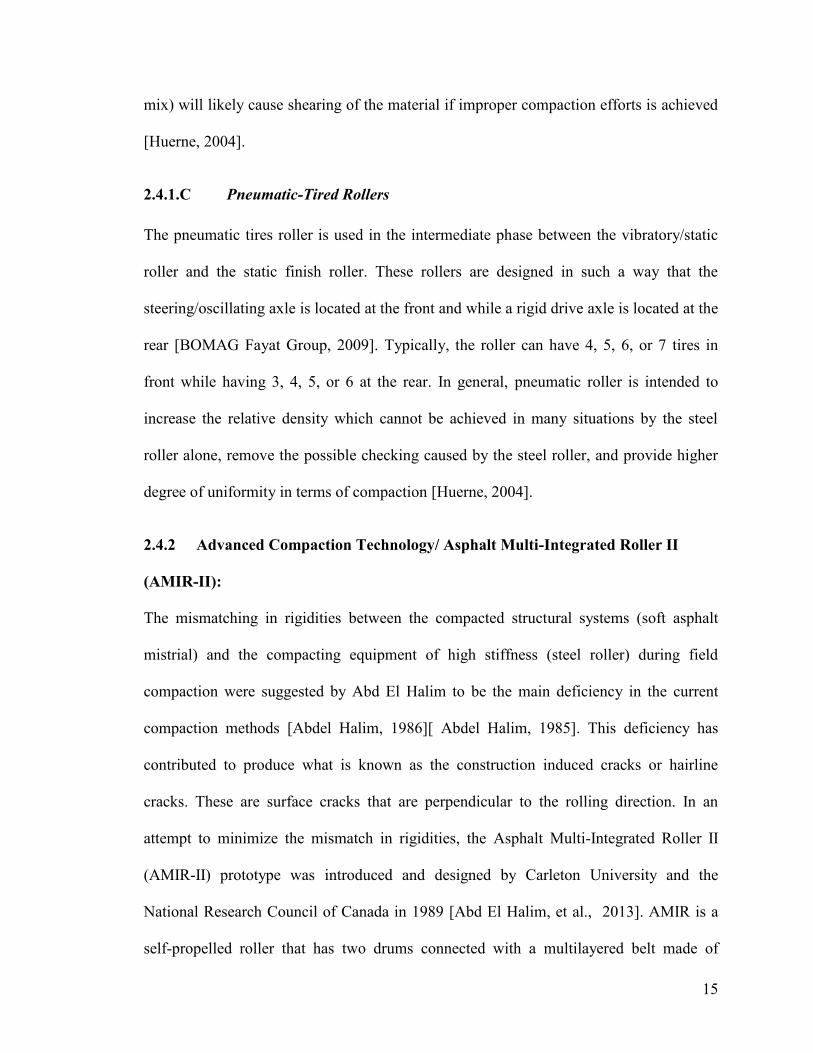
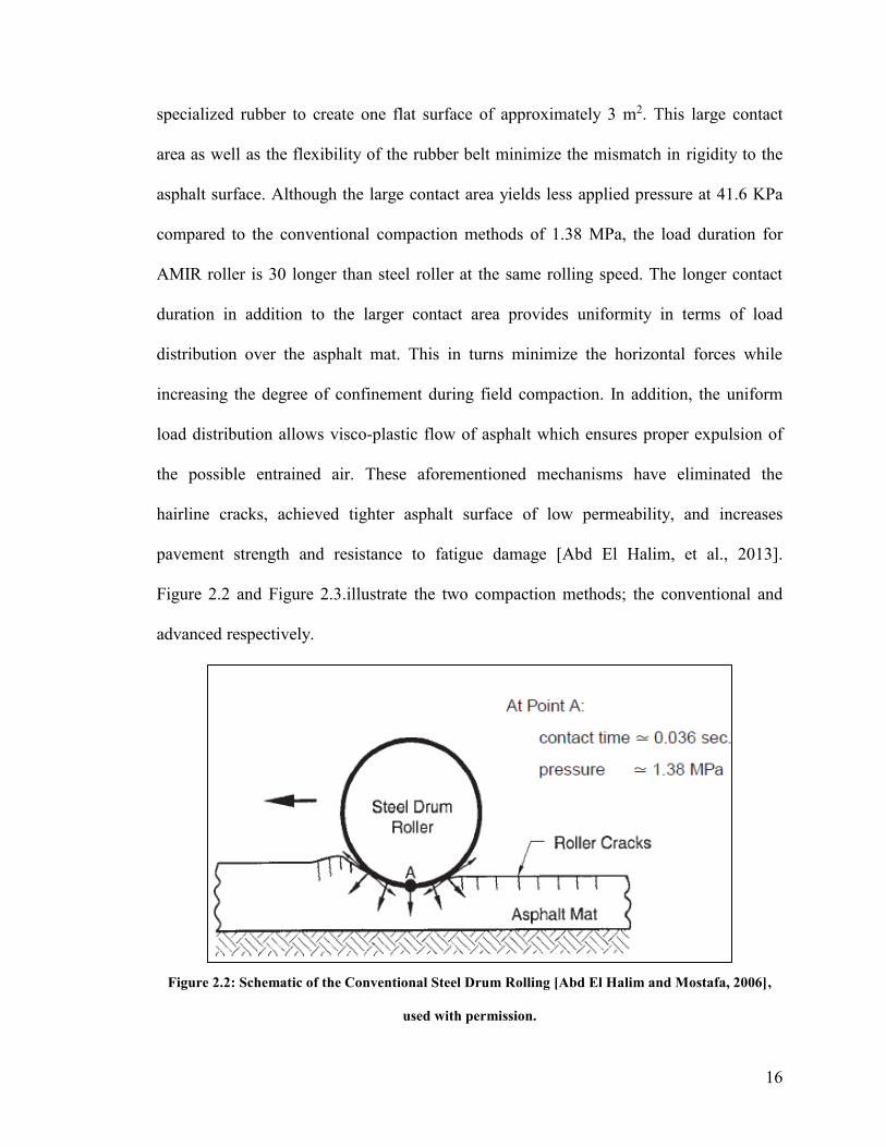
specialized rubber to create one flat surface of approximately 3 m2. This large contact
area as well as the flexibility of the rubber belt minimize the mismatch in rigidity to the
asphalt surface. Although the large contact area yields less applied pressure at 41.6 KPa
compared to the conventional compaction methods of 1.38 MPa, the load duration for
AMIR roller is 30 longer than steel roller at the same rolling speed. The longer contact
duration in addition to the larger contact area provides uniformity in terms of load
distribution over the asphalt mat. This in turns minimize the horizontal forces while
increasing the degree of confinement during field compaction. In addition, the uniform
load distribution allows visco-plastic flow of asphalt which ensures proper expulsion of
the possible entrained air. These aforementioned mechanisms have eliminated the
hairline cracks, achieved tighter asphalt surface of low permeability, and increases
pavement strength and resistance to fatigue damage [Abd El Halim, et al., 2013].
Figure 2.2 and Figure 2.3.illustrate the two compaction methods; the conventional and
advanced respectively.
Figure 2.2: Schematic of the Conventional Steel Drum Rolling [Abd El Halim and Mostafa, 2006],
used with permission.
17
Figure 2.3: Schematic of the Advanced Rolling [Abd El Halim and Mostafa, 2006], used with
permission
2.5 Permeability Testing Techniques
A number of devices and mechanisms are available in the literature for researchers and
practitioners to determine the pavement hydraulic conductivity (permeability). Some
apparatuses utilize the water as the fluid that will go through the pavement medium such
as the NCAT permeameter, others uses the air as the penetrating fluid such as the
Kentucky Air Induced permeameter [Allen, et al., 2003]. The techniques which some
devices are based on could also differ; the NCAT for example is based on the falling head
concept while the Kuss permeameter follows the constant head technique [Williams,
2006; Zaniewski and Yan, 2013; Hall, 2004]. This section of the literature is intended to
present the most common techniques to measure the pavement permeability to date. Also,
an evaluation and ranking of different field permeability testing methods will be carried
out in order to prioritize devices in terms of their practicality.
18
2.5.1 Field Devices
2.5.1.A NCAT Field Permeameter
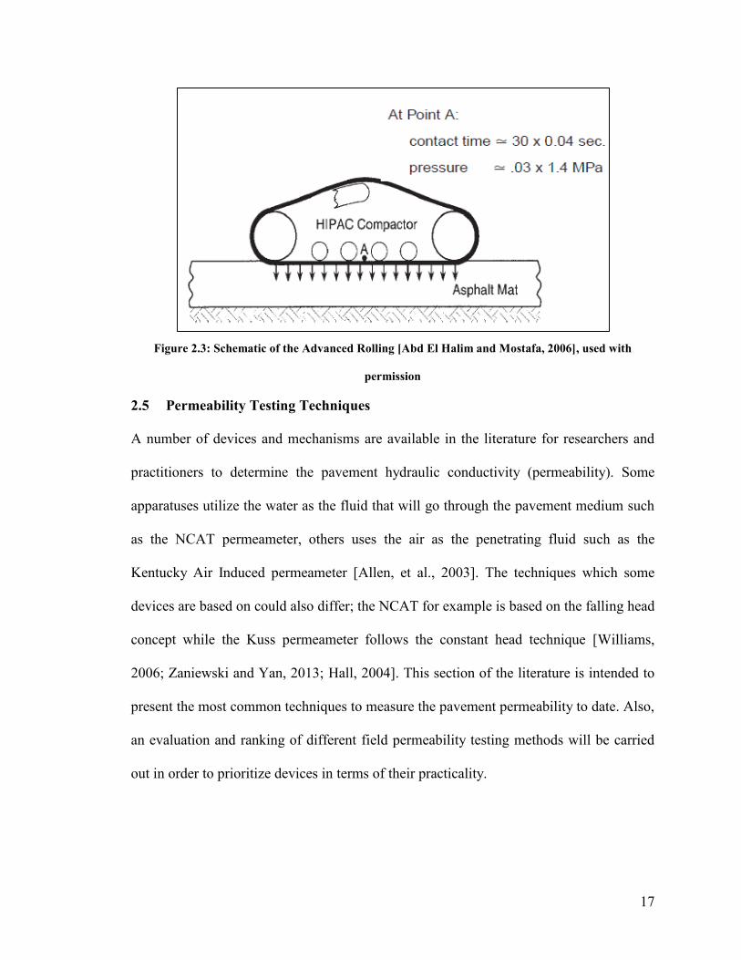
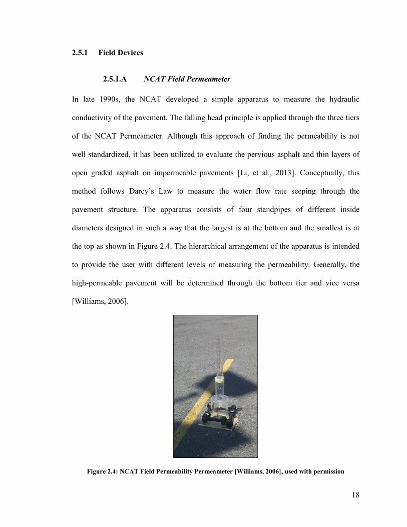
In late 1990s, the NCAT developed a simple apparatus to measure the hydraulic
conductivity of the pavement. The falling head principle is applied through the three tiers
of the NCAT Permeameter. Although this approach of finding the permeability is not
well standardized, it has been utilized to evaluate the pervious asphalt and thin layers of
open graded asphalt on impermeable pavements [Li, et al., 2013]. Conceptually, this
method follows Darcy’s Law to measure the water flow rate seeping through the
pavement structure. The apparatus consists of four standpipes of different inside
diameters designed in such a way that the largest is at the bottom and the smallest is at
the top as shown in Figure 2.4. The hierarchical arrangement of the apparatus is intended
to provide the user with different levels of measuring the permeability. Generally, the
high-permeable pavement will be determined through the bottom tier and vice versa
[Williams, 2006].
Figure 2.4: NCAT Field Permeability Permeameter [Williams, 2006], used with permission
19
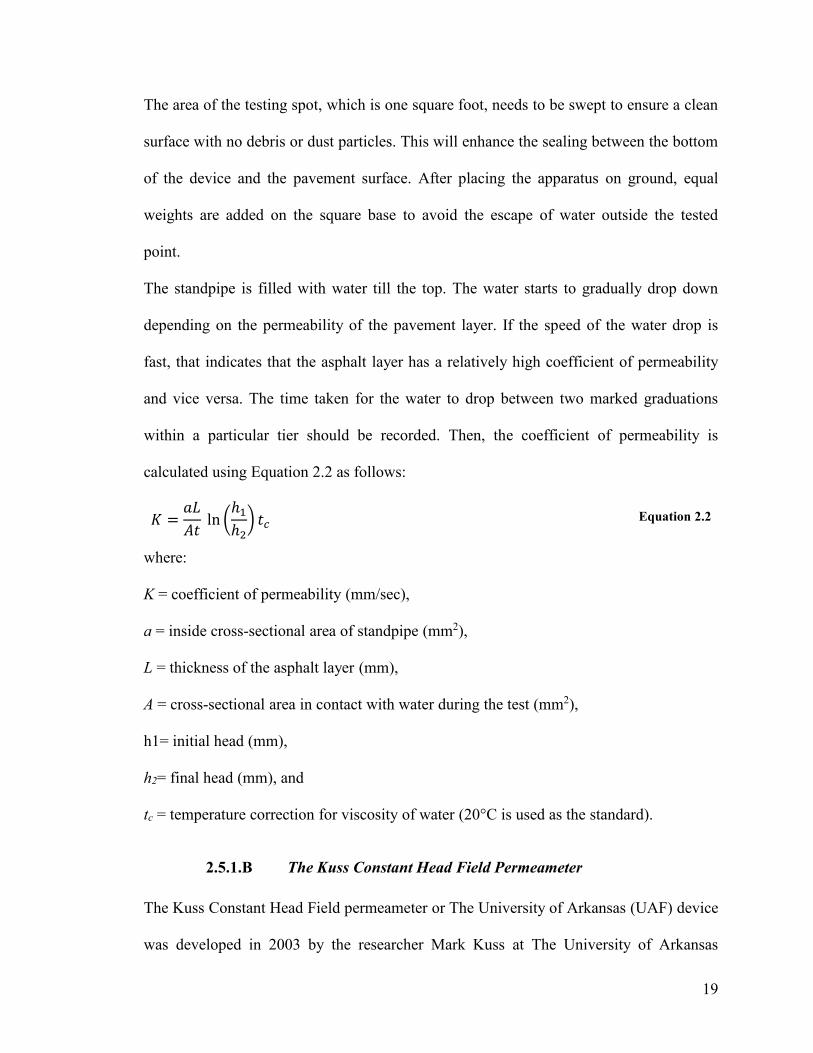
The area of the testing spot, which is one square foot, needs to be swept to ensure a clean
surface with no debris or dust particles. This will enhance the sealing between the bottom
of the device and the pavement surface. After placing the apparatus on ground, equal
weights are added on the square base to avoid the escape of water outside the tested
point.
The standpipe is filled with water till the top. The water starts to gradually drop down
depending on the permeability of the pavement layer. If the speed of the water drop is
fast, that indicates that the asphalt layer has a relatively high coefficient of permeability
and vice versa. The time taken for the water to drop between two marked graduations
within a particular tier should be recorded. Then, the coefficient of permeability is
calculated using Equation 2.2 as follows:
𝐾 =𝑎𝐿
𝐴𝑡 ln (
ℎ1
ℎ2) 𝑡𝑐 Equation 2.2
where:
K = coefficient of permeability (mm/sec),
a = inside cross-sectional area of standpipe (mm2),
L = thickness of the asphalt layer (mm),
A = cross-sectional area in contact with water during the test (mm2),
h1= initial head (mm),
h2= final head (mm), and
tc = temperature correction for viscosity of water (20°C is used as the standard).
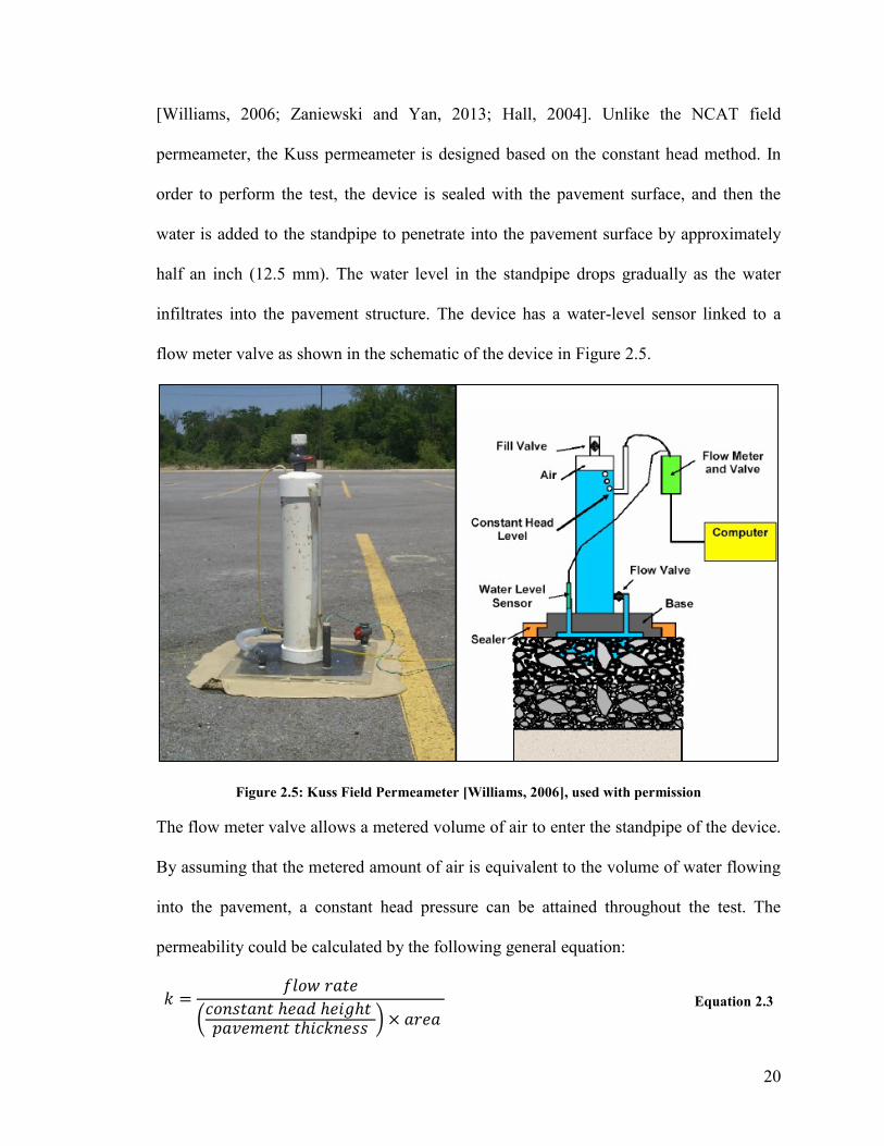
2.5.1.B The Kuss Constant Head Field Permeameter
The Kuss Constant Head Field permeameter or The University of Arkansas (UAF) device
was developed in 2003 by the researcher Mark Kuss at The University of Arkansas
20
[Williams, 2006; Zaniewski and Yan, 2013; Hall, 2004]. Unlike the NCAT field
permeameter, the Kuss permeameter is designed based on the constant head method. In
order to perform the test, the device is sealed with the pavement surface, and then the
water is added to the standpipe to penetrate into the pavement surface by approximately
half an inch (12.5 mm). The water level in the standpipe drops gradually as the water
infiltrates into the pavement structure. The device has a water-level sensor linked to a
flow meter valve as shown in the schematic of the device in Figure 2.5.
Figure 2.5: Kuss Field Permeameter [Williams, 2006], used with permission
The flow meter valve allows a metered volume of air to enter the standpipe of the device.
By assuming that the metered amount of air is equivalent to the volume of water flowing
into the pavement, a constant head pressure can be attained throughout the test. The
permeability could be calculated by the following general equation:
𝑘 =𝑓𝑙𝑜𝑤 𝑟𝑎𝑡𝑒
(𝑐𝑜𝑛𝑠𝑡𝑎𝑛𝑡 ℎ𝑒𝑎𝑑 ℎ𝑒𝑖𝑔ℎ𝑡 𝑝𝑎𝑣𝑒𝑚𝑒𝑛𝑡 𝑡ℎ𝑖𝑐𝑘𝑛𝑒𝑠𝑠
) × 𝑎𝑟𝑒𝑎 Equation 2.3
21
The water flow rate which is measured over time by a data acquisition system in the
device, the pavement cross-sectional area, and the pavement thickness are the needed
parameters to calculate permeability as presented in Equation 2.4.
𝑘 =𝑄
60 ×25.4 + 𝐿
𝐿 × 𝐴 Equation 2.4
where:
K = coefficient of permeability (mm/s),
Q = flow rate (mm3/min),
A = area of base plate (126450 mm2),
L = pavement thickness (mm),
60 = conversion factor from minutes to seconds, and
25.4 = conversion factor from inch to millimeter.
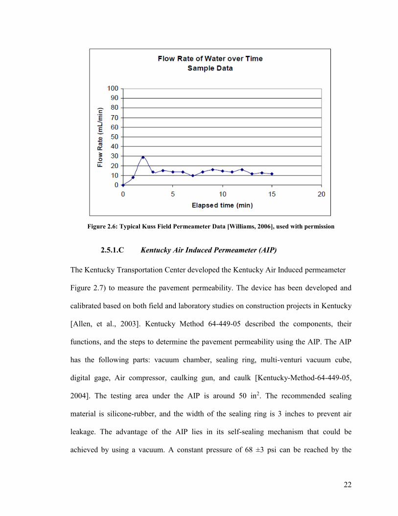
Since the device is connected to a computer, the results of the flow rate could be
generated automatically after conducting the test. A typical result is shown is Figure 2.6.
Normally, the steady-state flow condition will be achieved after a time period ranging
from 15 to 30 minutes.
22
Figure 2.6: Typical Kuss Field Permeameter Data [Williams, 2006], used with permission
2.5.1.C Kentucky Air Induced Permeameter (AIP)
The Kentucky Transportation Center developed the Kentucky Air Induced permeameter
Figure 2.7) to measure the pavement permeability. The device has been developed and
calibrated based on both field and laboratory studies on construction projects in Kentucky
[Allen, et al., 2003]. Kentucky Method 64-449-05 described the components, their
functions, and the steps to determine the pavement permeability using the AIP. The AIP
has the following parts: vacuum chamber, sealing ring, multi-venturi vacuum cube,
digital gage, Air compressor, caulking gun, and caulk [Kentucky-Method-64-449-05,
2004]. The testing area under the AIP is around 50 in2. The recommended sealing
material is silicone-rubber, and the width of the sealing ring is 3 inches to prevent air
leakage. The advantage of the AIP lies in its self-sealing mechanism that could be
achieved by using a vacuum. A constant pressure of 68 ±3 psi can be reached by the
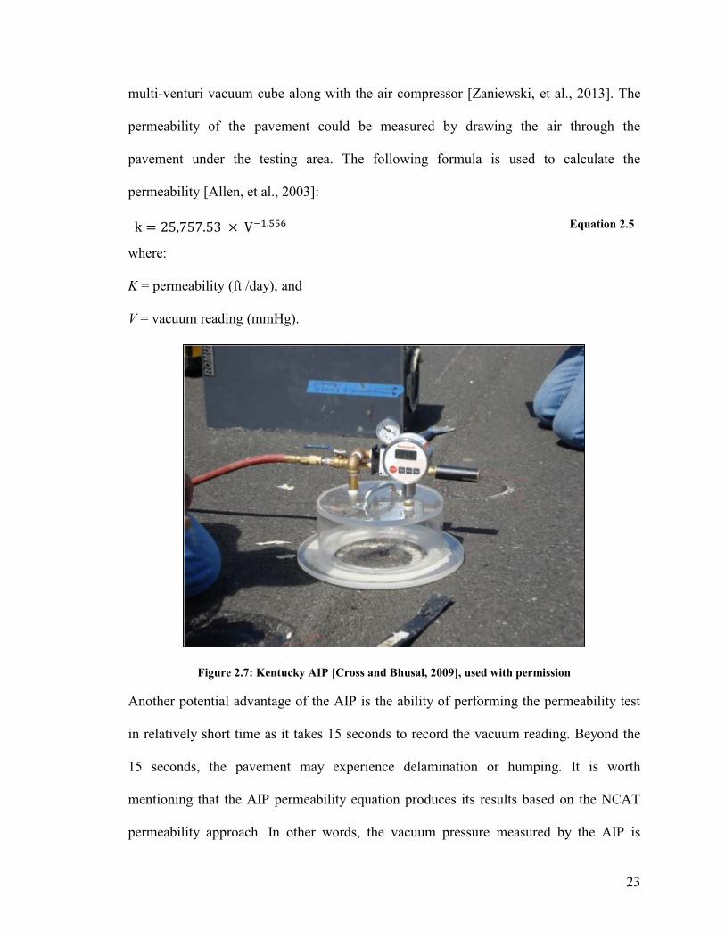
23
multi-venturi vacuum cube along with the air compressor [Zaniewski, et al., 2013]. The
permeability of the pavement could be measured by drawing the air through the
pavement under the testing area. The following formula is used to calculate the
permeability [Allen, et al., 2003]:
k = 25,757.53 × V−1.556 Equation 2.5
where:
K = permeability (ft /day), and
V = vacuum reading (mmHg).
Figure 2.7: Kentucky AIP [Cross and Bhusal, 2009], used with permission
Another potential advantage of the AIP is the ability of performing the permeability test
in relatively short time as it takes 15 seconds to record the vacuum reading. Beyond the
15 seconds, the pavement may experience delamination or humping. It is worth
mentioning that the AIP permeability equation produces its results based on the NCAT
permeability approach. In other words, the vacuum pressure measured by the AIP is
24
correlated to NCAT permeability. Another drawback of the method is the fact that the
AIP equation does not consider a temperature correction factor for viscosity of water as
the NCAT equation does. The testing procedures require a gasoline operated air
compressor or an electrical generator to be available in the field throughout the test which
might add some difficulties for test performance [Cross and Bhusal, 2009].
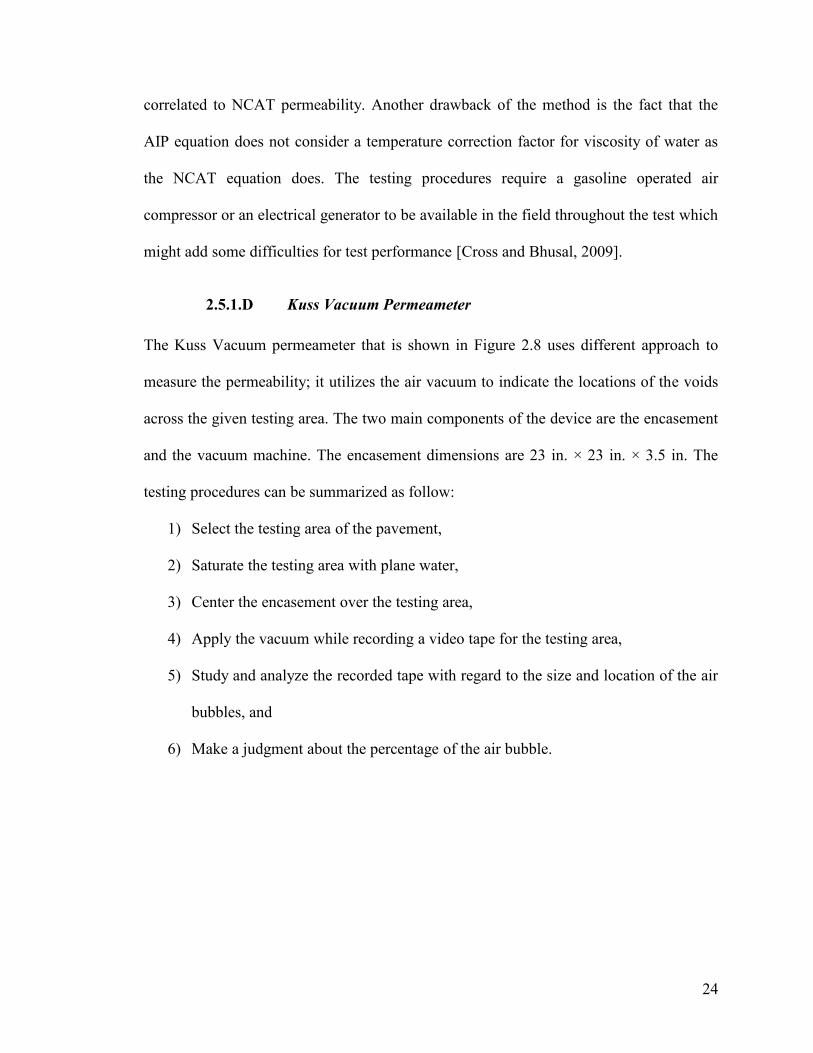
2.5.1.D Kuss Vacuum Permeameter
The Kuss Vacuum permeameter that is shown in Figure 2.8 uses different approach to
measure the permeability; it utilizes the air vacuum to indicate the locations of the voids
across the given testing area. The two main components of the device are the encasement
and the vacuum machine. The encasement dimensions are 23 in. × 23 in. × 3.5 in. The
testing procedures can be summarized as follow:
1) Select the testing area of the pavement,
2) Saturate the testing area with plane water,
3) Center the encasement over the testing area,
4) Apply the vacuum while recording a video tape for the testing area,
5) Study and analyze the recorded tape with regard to the size and location of the air
bubbles, and
6) Make a judgment about the percentage of the air bubble.
25
Figure 2.8: Kuss Vacuum Permeameter [Williams, 2006], used with permission
This method does not give the results of the permeability in the common forms but rather
reports it as a percentage (e.g. 24% air permeability) [Williams, 2006].
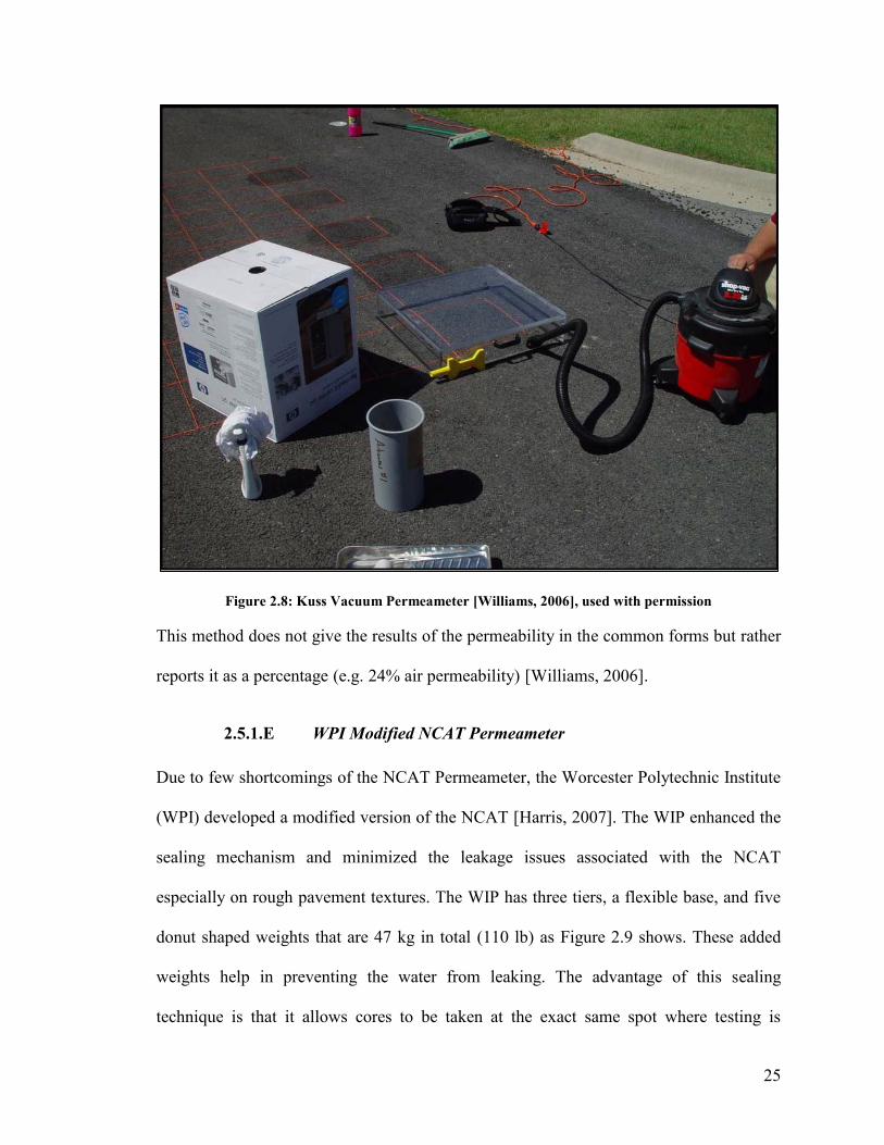
2.5.1.E WPI Modified NCAT Permeameter
Due to few shortcomings of the NCAT Permeameter, the Worcester Polytechnic Institute
(WPI) developed a modified version of the NCAT [Harris, 2007]. The WIP enhanced the
sealing mechanism and minimized the leakage issues associated with the NCAT
especially on rough pavement textures. The WIP has three tiers, a flexible base, and five
donut shaped weights that are 47 kg in total (110 lb) as Figure 2.9 shows. These added
weights help in preventing the water from leaking. The advantage of this sealing
technique is that it allows cores to be taken at the exact same spot where testing is
26
performed since the testing spot is not distorted by any marks or residuals of a sealant
materials. To read the initial and final head, a scale is attached to the top two tiers. In
order to establish a better sealing mechanism, the developer selected a flexible closed-cell
sponge rubber to be used at the base of the device. This rubber has two advantages; first
its non-absorptive nature, second its ability to prevent flow of water through the
macrostructure of the pavement surface [Mallick, et al., 2003].
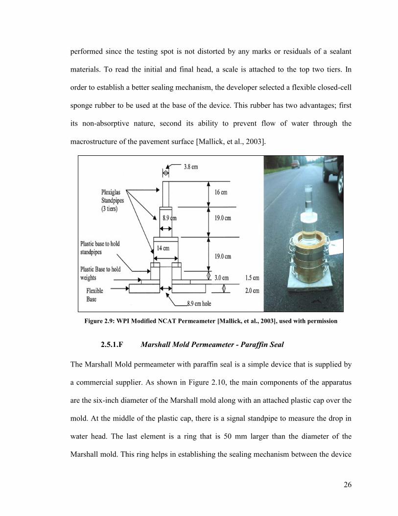
Figure 2.9: WPI Modified NCAT Permeameter [Mallick, et al., 2003], used with permission
2.5.1.F Marshall Mold Permeameter - Paraffin Seal
The Marshall Mold permeameter with paraffin seal is a simple device that is supplied by
a commercial supplier. As shown in Figure 2.10, the main components of the apparatus
are the six-inch diameter of the Marshall mold along with an attached plastic cap over the
mold. At the middle of the plastic cap, there is a signal standpipe to measure the drop in
water head. The last element is a ring that is 50 mm larger than the diameter of the
Marshall mold. This ring helps in establishing the sealing mechanism between the device

27
and the pavement surface. The unique sealing mechanism of this device embodied in
using the paraffin to prevent the water leakage. The paraffin has been selected because of
its physical nature that has two main advantages. The paraffin physical state shifts from
liquid to solid in a relatively short time. In the liquid stage, the paraffin will fill all the
voids and the pores between the pavement and the device [Cooley, 1999].
Figure 2.10: Marshall Mold Permeameter Paraffin Seal [Cooley, 1999], used with permission
This method requires a well-trained user to perform the test. Heating and cooling down of
the paraffin to the desirable degree of hardening is a challenging task. If the paraffin did
not cool properly before the pouring stage, it would flow under the edges of the device
and clog the flow paths. On the other hand, if the paraffin overly cooled, it would get
stiffer fast and would not provide a good sealing [Williams, 2006; Harris, 2007].
28
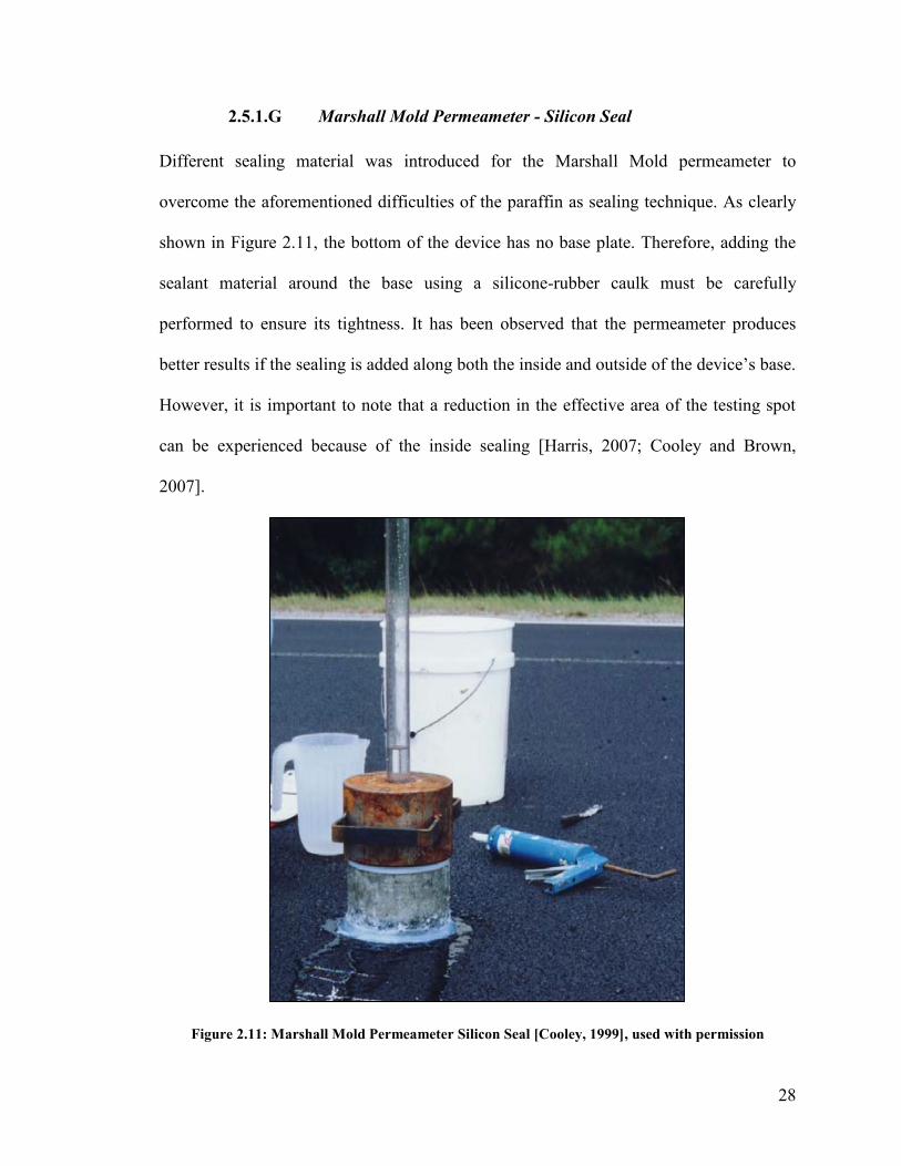
2.5.1.G Marshall Mold Permeameter - Silicon Seal
Different sealing material was introduced for the Marshall Mold permeameter to
overcome the aforementioned difficulties of the paraffin as sealing technique. As clearly
shown in Figure 2.11, the bottom of the device has no base plate. Therefore, adding the
sealant material around the base using a silicone-rubber caulk must be carefully
performed to ensure its tightness. It has been observed that the permeameter produces
better results if the sealing is added along both the inside and outside of the device’s base.
However, it is important to note that a reduction in the effective area of the testing spot
can be experienced because of the inside sealing [Harris, 2007; Cooley and Brown,
2007].
Figure 2.11: Marshall Mold Permeameter Silicon Seal [Cooley, 1999], used with permission
29
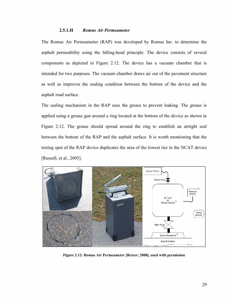
2.5.1.H Romus Air Permeameter
The Romus Air Permeameter (RAP) was developed by Romus Inc. to determine the
asphalt permeability using the falling-head principle. The device consists of several
components as depicted in Figure 2.12. The device has a vacuum chamber that is
intended for two purposes. The vacuum chamber draws air out of the pavement structure
as well as improves the sealing condition between the bottom of the device and the
asphalt road surface.
The sealing mechanism in the RAP uses the grease to prevent leaking. The grease is
applied using a grease gun around a ring located at the bottom of the device as shown in
Figure 2.12. The grease should spread around the ring to establish an airtight seal
between the bottom of the RAP and the asphalt surface. It is worth mentioning that the
testing spot of the RAP device duplicates the area of the lowest tier in the NCAT device
[Russell, et al., 2005].
Figure 2.12: Romus Air Permeameter [Retzer, 2008], used with permission
30
At the beginning of the test, the device should be sealed properly at the targeted location.
Prior to starting the test, if the pressure of the device is not appropriately set, the air tank
is pressurized to a head of 24 inches. The test begins once the “Start” button of the device
is pressed. Subsequently, a fully automated system is activated where a pressure sensor
monitors the pressure in the tank while the air is drawn through the pavement. The only
output of the device is the time of head drop which is recorded for each 4 inches of
pressure drop. Researchers at Marquette University have found out that the RAP
produces consistent results for different testing locations [Russell, et al., 2005]. By using
the time, thickness of the pavement layer, and other constant parameters, one can use
Equation 2.6 to find the pavement permeability:
𝑘𝑤 = [𝐿𝑉𝜇𝜌𝑤𝑔
𝑇𝐴𝑃𝑎𝜇𝑤] × ln [
𝑃1
𝑃2] Equation 2.6
where:
Kw = hydraulic permeability (L/T),
L = pavement layer thickness (L),
V = volume of vacuum chamber (L3),
μ = kinematic viscosity of air (M/LT),
ρw = density of water (M/L3),
g= gravitational acceleration (L/T2),
T = time of head drop (T),
A = area of being tested (L2),
Pa = pressure (atmospheric) (F/L2),
μw = kinematic viscosity of water (M/LT),
p1 = initial pressure (L), and
p2 = final pressure (L).
31
2.5.2 Ranking and Evaluation of Field Test:
As presented in the previous section, there are numerous techniques that are used to
measure the permeability in the literature; these methods differ in their mechanism,
reliability, and outcomes. This section is indented to evaluate and rank all the common
permeability techniques based on some criteria which are device usability, testing speed,
consistency, laboratory correlation, and purchasing cost. Each criterion will be given a
weight based on its importance as follows:
A = 5 (Very important)
B = 4 (Important)
C = 3 (Moderate)
D = 2 (Less important)
E = 1 (Not important)
Each device will be assessed a score ranging from 0 (lowest score) to 10 (highest score)
for each corresponding criterion. The formula that will be used to calculate the
performance index for each device is
The Marshall Mold permeameter with paraffin seal is excluded from the evaluation and
ranking processes because the device was found to be extremely difficult to be operated
in the field as concluded by Cooley [Cooley, 1999]. Table 2.2 shows the seven
considered devices for evaluation and their corresponding score for each criterion. These
scores were given to each device based on the review of the literature. On the basis of the
results of Table 2.2, it is shown that the most suitable and practical permeameter to be
𝑃𝑒𝑟𝑓𝑜𝑟𝑚𝑎𝑛𝑐𝑒 𝐼𝑛𝑑𝑒𝑥 = ∑(𝐶𝑟𝑖𝑡𝑒𝑟𝑖𝑜𝑛 𝑊𝑒𝑖𝑔ℎ𝑡) × (𝐷𝑒𝑣𝑖𝑐𝑒 𝑆𝑐𝑜𝑟𝑒)
∑ 𝐶𝑟𝑖𝑡𝑒𝑟𝑖𝑎 𝑊𝑒𝑖𝑔ℎ𝑡 Equation 2.7
32
used by the QA/QC practitioners is the NCAT permeameter. The ranking for all devices
is presented in Table 2.3.
Table 2.2: Comparison Matrix for All the Permeability Devices
Criterion Name Ease of
Use
Test
Speed
Consistency
In Results
Correlation
With The
Lab Results
Cost Overall
Score
Criterion Weight Moderate Important Very
Important Important
Less
Important
Device Name
The Kuss Permeameter 7 5 8 8 N/A 7.06
Kentucky Permeameter (AIP) 8 8 7 5 N/A 6.94
NCAT Permeameter 7 8 6 8 8 7.28
Kuss Vacuum Permeameter 5 4 8 N/A N/A 5.92
WPI modified NCAT 7 7 4 N/A N/A 5.75
Romus Air Permeameter 4 8 4 5 3 5.00
Marshall Mold (Silicon Seal) 6 7 6 8 N/A 6.75
(N/A): No score was given as no conclusions were found in the literature
Table 2.3: Field Permeameter Ranking
Device Overall Score
NCAT Permeameter 7.28
The Kuss Permeameter 7.06
Kentucky Permeameter (AIP) 6.94
Marshall Mold (Silicon Seal) 6.75
Kuss Vacuum Permeameter 5.92
WPI modified NCAT 5.75
Romus Air Permeameter 5.00
As previously stated, it has been found that the most common device for performing the
hydraulic conductivity test in the field is the NCAT apparatus. This is due to its ease of
use, short time of the test, and nondestructive nature. However, there are few drawbacks
of this method that should be mentioned based on field observations. It is almost a
33
challenging task to create a tight sealant between the pavement surface and the bottom of
the NCAT device especially when the pavement surface is not smooth. Generally, rough
pavement surface will promote more water leakage. This is due to the fact that the sealed
material (putty) gets wet with time and allows the water to leak through its rough surface.
A recent study proposed a new sealing material to be used to overcome the leaking issue.
The study recommended the use of the “Ecoflex 5 silicone rubber by Smooth-On®”
along with the caulking gun [Li, et al., 2013]. Also, the NCAT manual instructs the user
to add some weights to the base of the device to have a better sealing. However, there is
no defined standard weight that will guarantee a solution to leakage problem.
2.5.3 Laboratory Devices
2.5.3.A Karol-Warner Asphalt Permeameter
The common laboratory method that is adopted to measure the coefficient of permeability
for HMA cores or laboratory prepared specimens was developed by the Florida
Department of Transportation (FDOT) in 1996 [James, et al., 2004] This test method
(Figure 2.13) has been selected as the standard lab test for measuring permeability and
the procedure is outlined in ASTM PS 129-01, Permeability of Bituminous Materials
[Zaniewski and Yan, 2013]. The method follows the falling head principle to measure the
coefficient of permeability. Water is allowed to drop in the graduated cylinder passing
through a saturated asphalt sample. The initial water head, the final water head, and the
time interval between the two heads are recorded and used for permeability calculations
based on Darcy’s law [Florida Test Method, 1997] The testing producer was then slightly
modified by recommending an epoxy resin to seal the sidewalls of the core when using
the flexible latex membrane [Mallick, et al., 2003]. To represent a better simulation of the
34
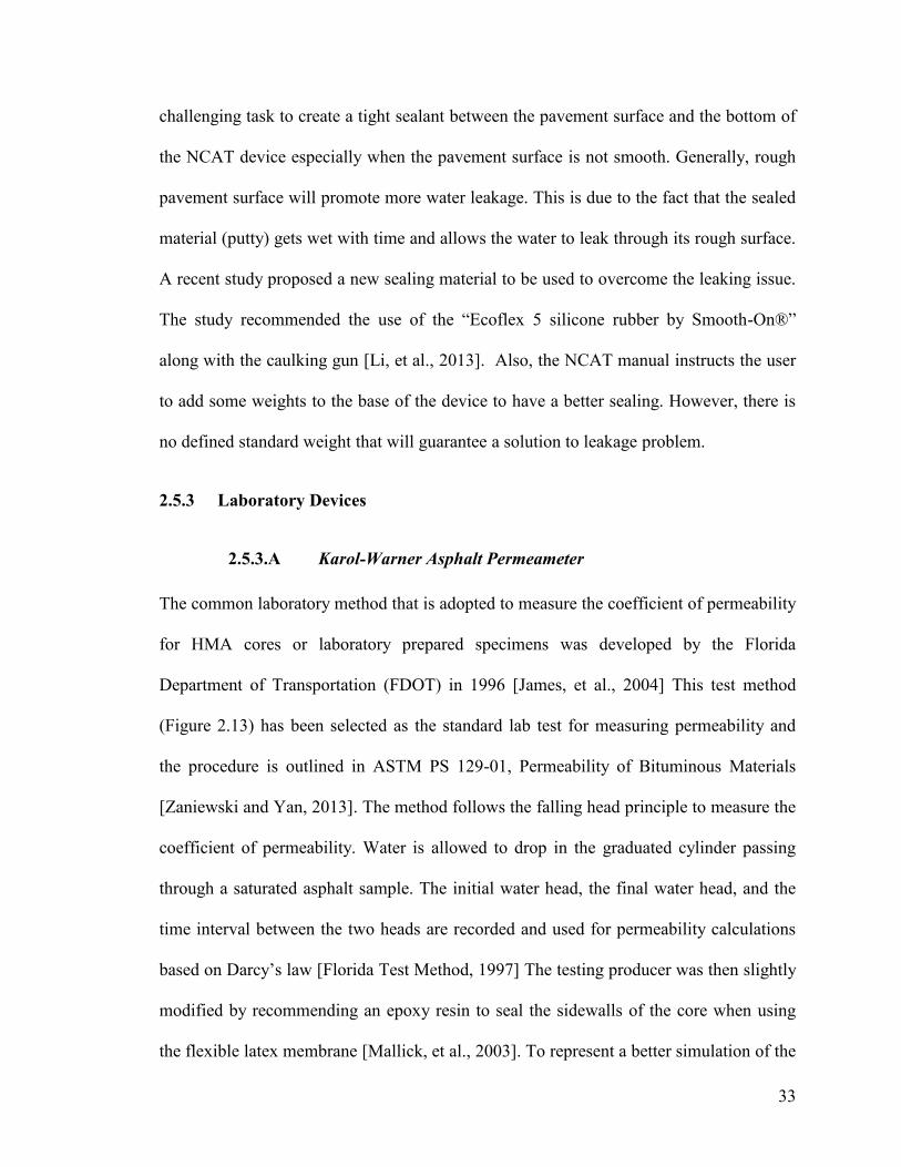
in-situ permeability, the ASTM subcommittee D.423 modified the testing apparatus by
adding a rising tail element that acts as an outlet pipe for the penetrated water through the
specimen.
Figure 2.13: The Laboratory Permeability Device
This test is applicable for both field cores along with laboratory prepared specimens
[Zaniewski and Yan, 2013]. The testing permeameter consists of a vertical standpipe, two
expandable sealing rings, a six inch aluminum containment cylinder, a latex membrane, a
water release valve, and a manual air pump with a pressure gauge. The testing specimen
is placed on the chamber. Then the latex membrane is pressurized to prevent water
passing through the sides of the sample. The specimen should reach a saturation
35
condition by allowing a 500 ml of water to pass through it twice. The difference in the
water flow rate should not be more than 4% to assure the saturation condition. The
standpipe is then filled with water and the valve is released. The time is then recorded for
the water level to move from the initial head value to the final head value [Florida Test
Method, 1997]. More details about his test will be presented later at Section 3.2.2.
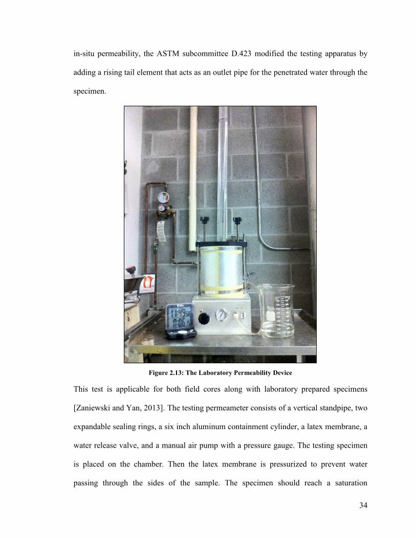
2.5.3.B Corelok Device
The coefficient of permeability for HMA specimens can be determined through
quantifying the percentage of porosity for a particular asphalt sample. The CoreLok
device (Figure 2.14) can be used to measure the porosity for HMA samples which can be
used to find the permeability value. One finding suggests that this method is better for
determining permeability because two samples with the same percent porosity will have
almost the same permeability value [Harris, 2007]. In general, for a coarse-graded
mixture, measuring the porosity is much more representative rather than the air voids. In
contrast, the air voids for dense-graded or fine mixtures is relatively sufficient to indicate
the sample condition for quality control and QA purposes. The porosity accounts for the
air voids content, size, and interconnectedness within a given sample [Vivar and
Haddocl, 2006]. Generally, it has been concluded that the permeability is a good indicator
of voids that are exposed to water, while porosity is good at indicating all voids whether
they are accessible by water or not [Çelik, 2005].
The procedures that are required to find the porosity value begin by placing the sample in
a vacuum-sealed bag to determine its density “ρ1”. Then, the sample should be covered
and placed under water, then the bag covering the sample should be opened while
maintaining the submerged condition; this is necessary to quantify its underwater density
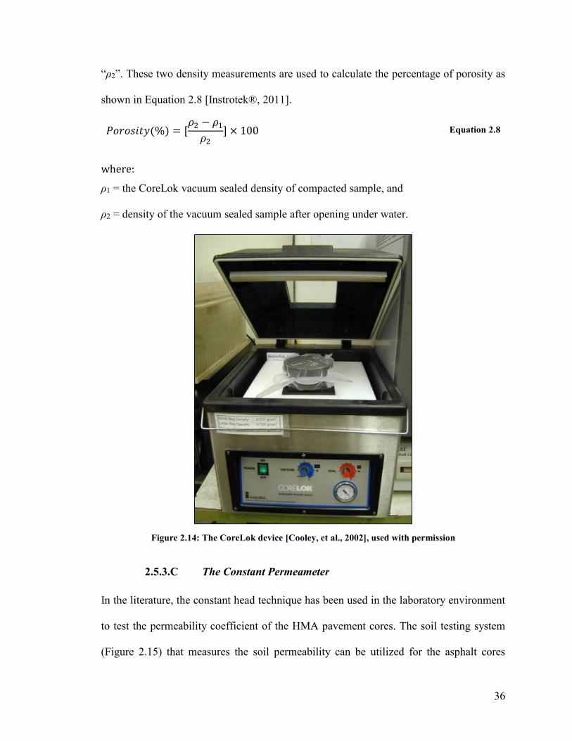
36
“ρ2”. These two density measurements are used to calculate the percentage of porosity as
shown in Equation 2.8 [Instrotek®, 2011].
𝑃𝑜𝑟𝑜𝑠𝑖𝑡𝑦(%) = [𝜌2 − 𝜌1
𝜌2] × 100 Equation 2.8
where:
ρ1 = the CoreLok vacuum sealed density of compacted sample, and
ρ2 = density of the vacuum sealed sample after opening under water.
Figure 2.14: The CoreLok device [Cooley, et al., 2002], used with permission
2.5.3.C The Constant Permeameter
In the literature, the constant head technique has been used in the laboratory environment
to test the permeability coefficient of the HMA pavement cores. The soil testing system
(Figure 2.15) that measures the soil permeability can be utilized for the asphalt cores
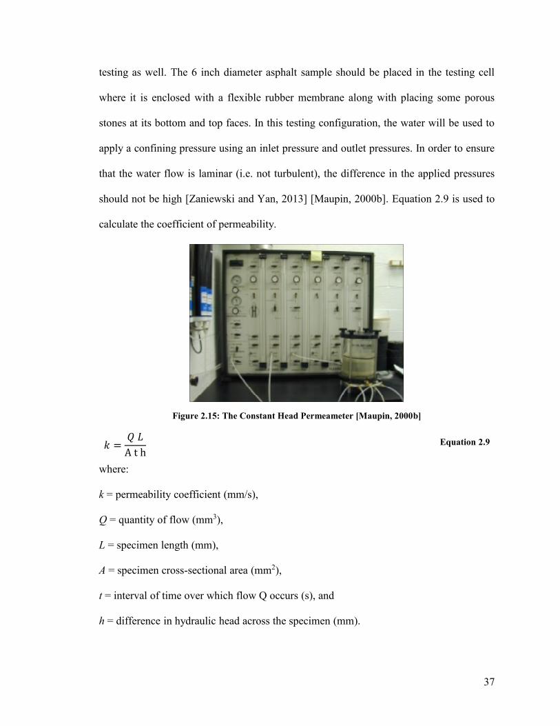
37
testing as well. The 6 inch diameter asphalt sample should be placed in the testing cell
where it is enclosed with a flexible rubber membrane along with placing some porous
stones at its bottom and top faces. In this testing configuration, the water will be used to
apply a confining pressure using an inlet pressure and outlet pressures. In order to ensure
that the water flow is laminar (i.e. not turbulent), the difference in the applied pressures
should not be high [Zaniewski and Yan, 2013] [Maupin, 2000b]. Equation 2.9 is used to
calculate the coefficient of permeability.
Figure 2.15: The Constant Head Permeameter [Maupin, 2000b]
𝑘 =𝑄 𝐿
A t h Equation 2.9
where:
k = permeability coefficient (mm/s),
Q = quantity of flow (mm3),
L = specimen length (mm),
A = specimen cross-sectional area (mm2),
t = interval of time over which flow Q occurs (s), and
h = difference in hydraulic head across the specimen (mm).
38
CHAPTER 3: EXPERIMENTAL PROGRAM
The planned and implemented experimental program in this study consisted of two major
phases. The first phase dealt with the measurements of in-situ permeability of newly
constructed asphalt pavement surfaces and in-service roads. The term “in-service” refers
to sites that were compacted and tested in a previous year. In addition, field cores were
recovered from each test location for performing a major portion of the second phase.
The second phase is mainly based on laboratory investigations including preparing
laboratory specimens using loose mixtures provided by the MTO along with performing
different laboratory tests. In particular, the laboratory experimental program involved
measuring the relative density, IDT, and laboratory permeability of the field-recovered
cores as well as laboratory prepared specimens. Figure 3.1 illustrates the major
components of the experimental investigation carried out in this research.
3.1 Data Collection
Several sites (highway projects and in-house field trials) in Ontario’s Eastern Region
were selected for inspection and sampling immediately after the paving and the
compaction stages are completed. The term “in-house” is used in this research to refer to
non-highway field projects performed at controlled locations/sections under the
supervision of the construction firm R.W.Tomlinson Limited. Other in-service highway
sections were also investigated to evaluate the effect of age and traffic on the
permeability of the road surface. The testing program included sites finished by two
different compaction methods including the advanced and the conventional compaction
techniques to examine the effect of compaction on the mechanical and physical properties
of asphalt pavement.
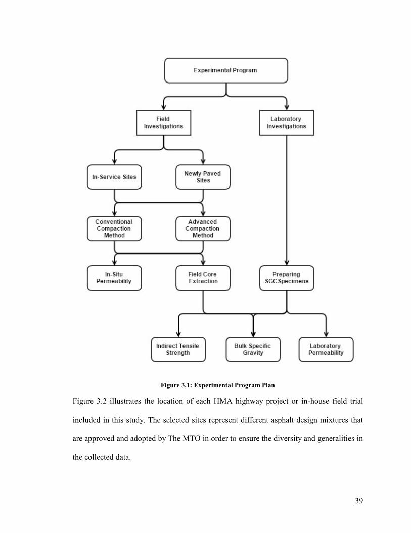
39
Figure 3.1: Experimental Program Plan
Figure 3.2 illustrates the location of each HMA highway project or in-house field trial
included in this study. The selected sites represent different asphalt design mixtures that
are approved and adopted by The MTO in order to ensure the diversity and generalities in
the collected data.
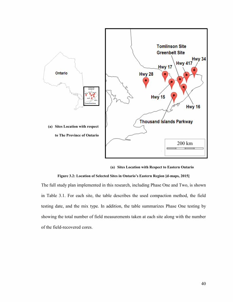
40
(a) Sites Location with respect
to The Province of Ontario
(a) Sites Location with Respect to Eastern Ontario
Figure 3.2: Location of Selected Sites in Ontario’s Eastern Region [d-maps, 2015]
The full study plan implemented in this research, including Phase One and Two, is shown
in Table 3.1. For each site, the table describes the used compaction method, the field
testing date, and the mix type. In addition, the table summarizes Phase One testing by
showing the total number of field measurements taken at each site along with the number
of the field-recovered cores.
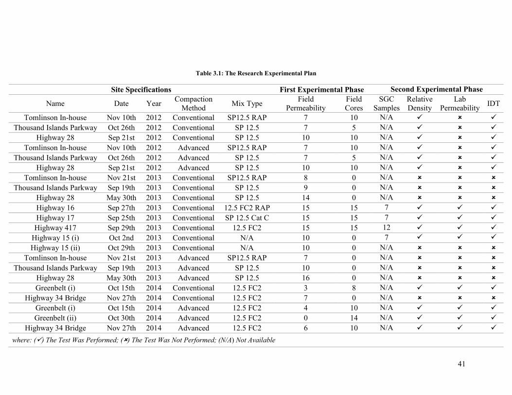
41
Table 3.1: The Research Experimental Plan
Site Specifications First Experimental Phase Second Experimental Phase
Name Date Year Compaction
Method Mix Type
Field
Permeability
Field
Cores
SGC
Samples
Relative
Density
Lab
Permeability IDT
Tomlinson In-house Nov 10th 2012 Conventional SP12.5 RAP 7 10 N/A
Thousand Islands Parkway Oct 26th 2012 Conventional SP 12.5 7 5 N/A
Highway 28 Sep 21st 2012 Conventional SP 12.5 10 10 N/A
Tomlinson In-house Nov 10th 2012 Advanced SP12.5 RAP 7 10 N/A
Thousand Islands Parkway Oct 26th 2012 Advanced SP 12.5 7 5 N/A
Highway 28 Sep 21st 2012 Advanced SP 12.5 10 10 N/A
Tomlinson In-house Nov 21st 2013 Conventional SP12.5 RAP 8 0 N/A
Thousand Islands Parkway Sep 19th 2013 Conventional SP 12.5 9 0 N/A
Highway 28 May 30th 2013 Conventional SP 12.5 14 0 N/A
Highway 16 Sep 27th 2013 Conventional 12.5 FC2 RAP 15 15 7
Highway 17 Sep 25th 2013 Conventional SP 12.5 Cat C 15 15 7
Highway 417 Sep 29th 2013 Conventional 12.5 FC2 15 15 12
Highway 15 (i) Oct 2nd 2013 Conventional N/A 10 0 7
Highway 15 (ii) Oct 29th 2013 Conventional N/A 10 0 N/A
Tomlinson In-house Nov 21st 2013 Advanced SP12.5 RAP 7 0 N/A
Thousand Islands Parkway Sep 19th 2013 Advanced SP 12.5 10 0 N/A
Highway 28 May 30th 2013 Advanced SP 12.5 16 0 N/A
Greenbelt (i) Oct 15th 2014 Conventional 12.5 FC2 3 8 N/A
Highway 34 Bridge Nov 27th 2014 Conventional 12.5 FC2 7 0 N/A
Greenbelt (i) Oct 15th 2014 Advanced 12.5 FC2 4 10 N/A
Greenbelt (ii) Oct 30th 2014 Advanced 12.5 FC2 0 14 N/A
Highway 34 Bridge Nov 27th 2014 Advanced 12.5 FC2 6 10 N/A
where: () The Test Was Performed; () The Test Was Not Performed; (N/A) Not Available
42
It can been seen that all included sites in this research have common nominal maximum
aggregate size (NMAS) of 12.5 mm. Table 3.1 summarizes also the second experimental
phase by showing the incorporated laboratory tests on the field-recovered cores as well as
the SGC specimens of each site. It is important to mention that in some cases the number
of the field-recovered cores might not be the same as the number of the field
measurements. The time limitations of the road closure provided by the traffic control
technicians, the time restriction/availability of the core drilling operator, or performing
the field test and field coring in different days were behind not having the same number
of field measurements and field-recovered cores. However, having shortage or surplus in
the number of field cores with respect to the field measurements does not violate the fact
that the field cores were extracted from the same in-situ tested location.
The field testing involved performing the in-situ permeability measurements at specific
locations along and across the road sections. In addition, asphalt cores were extracted
from the same locations where the in-situ measurements were taken. The testing program
used the same field testing device at all sites. In particular, the in-situ permeability testing
protocol was performed using the NCAT permeameter at each of the selected sites. As
explained earlier in Chapter 2, this was the method recommended in this research based
on the evaluation of available field permeability measurement techniques in the literature.
At each investigated site a total of three to five testing spots were selected along the
cross-section of a lane on each selected site to examine the variability in permeability
with the change of lateral location of the testing location. For each testing spot (diameter
= 150 mm), a pavement core was then recovered and transported to the Civil Engineering
43
Laboratory at Carleton University for further experimental investigations as explained
earlier.
Figure 3.3 illustrates the testing locations incorporated in this research and their
corresponding distances from the centerline of the paved lane. Relative to the centerline
of the selected site lane:
The first testing location was at 200 mm and termed “Inner Edge”,
The second was at 850 mm and termed “Inner Middle”,
The third was at 1900 mm and termed “Middle”,
The fourth was at 2750 mm and termed “Outer Middle” and
The fifth was at 3400 mm and termed “Outer”.
In certain sites and due to limitations of time and safety considerations of the research
team, the in-situ permeability measurements were limited to three testing locations; the
outer, middle and inner. In other sites where more testing time was allowed by the traffic
control workers, all five locations were covered. As stated previously, the main reason of
performing the permeability test at different locations was to ensure covering as wide
area of the paved lane as possible and to assess the possible variability in density,
permeability and strength values.
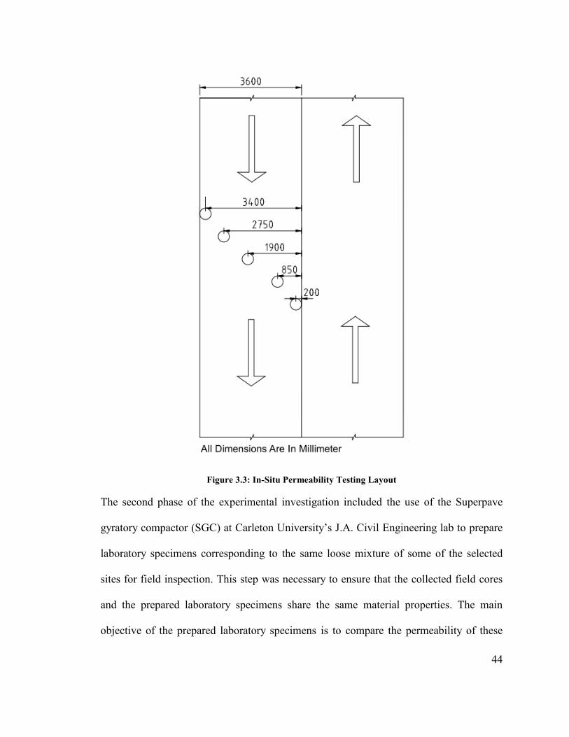
44
Figure 3.3: In-Situ Permeability Testing Layout
The second phase of the experimental investigation included the use of the Superpave
gyratory compactor (SGC) at Carleton University’s J.A. Civil Engineering lab to prepare
laboratory specimens corresponding to the same loose mixture of some of the selected
sites for field inspection. This step was necessary to ensure that the collected field cores
and the prepared laboratory specimens share the same material properties. The main
objective of the prepared laboratory specimens is to compare the permeability of these
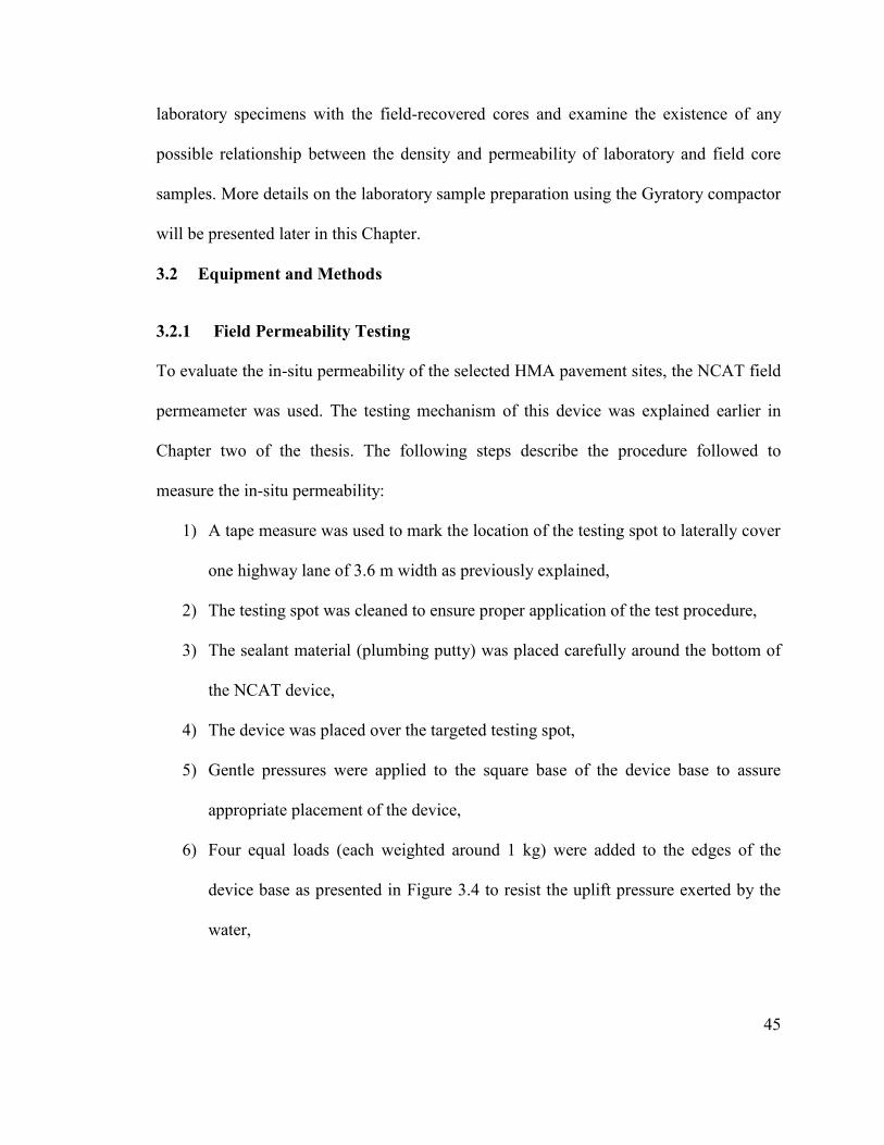
45
laboratory specimens with the field-recovered cores and examine the existence of any
possible relationship between the density and permeability of laboratory and field core
samples. More details on the laboratory sample preparation using the Gyratory compactor
will be presented later in this Chapter.
3.2 Equipment and Methods
3.2.1 Field Permeability Testing
To evaluate the in-situ permeability of the selected HMA pavement sites, the NCAT field
permeameter was used. The testing mechanism of this device was explained earlier in
Chapter two of the thesis. The following steps describe the procedure followed to
measure the in-situ permeability:
1) A tape measure was used to mark the location of the testing spot to laterally cover
one highway lane of 3.6 m width as previously explained,
2) The testing spot was cleaned to ensure proper application of the test procedure,
3) The sealant material (plumbing putty) was placed carefully around the bottom of
the NCAT device,
4) The device was placed over the targeted testing spot,
5) Gentle pressures were applied to the square base of the device base to assure
appropriate placement of the device,
6) Four equal loads (each weighted around 1 kg) were added to the edges of the
device base as presented in Figure 3.4 to resist the uplift pressure exerted by the
water,
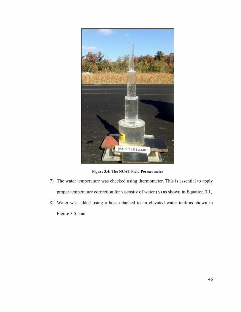
46
Figure 3.4: The NCAT Field Permeameter
7) The water temperature was checked using thermometer. This is essential to apply
proper temperature correction for viscosity of water (tc) as shown in Equation 3.1,
8) Water was added using a hose attached to an elevated water tank as shown in
Figure 3.5, and
47
Figure 3.5: In-situ Permeability Test at Highway 16 Project
9) The time required for the water to drop from the top graduation mark (660 mm) of
the tier with the smallest diameter to the bottom mark (520 mm) of the same tier
was recorded.
In some cases where testing locations experienced relatively excessive permeability,
causing water to drop fast in the first tier, the next tier was used. During the field
investigations, any testing location that exhibited any water leakage signs was discarded
and repeated elsewhere. Core extraction was performed on the exact location where the
field permeability test was conducted. The coefficient of permeability was calculated
using Equation 3.1. In all sites, the thickness of the asphalt layer (L) was estimated by
measuring the thickness of the field-recovered cores.

48
𝑘 =𝑎𝐿
Atln (
ℎ1
ℎ2)𝑡𝑐 Equation 3.1
where:
K = coefficient of permeability (mm/sec),
a = inside cross-section area of standpipe (mm2),
L = thickness of the asphalt layer (mm),
A = circular cross-sectional area of tested pavement (mm2),
h1 = initial head (mm),
h2 = final head (mm),
t = elapsed time between h1 and h2 (sec), and
tc = temperature correction for viscosity of water (20°C is used as the standard).
3.2.2 Laboratory Permeability Testing
The laboratory permeability (hydraulic conductivity) of the test specimen was estimated
using the Karol-Warner Asphalt permeameter that is shown in Figure 3.6. In this study,
the Florida Test Method (FM 5-565) was followed to determine the laboratory
permeability values [Florida Test Method, 2012]. Similar to the NCAT mechanism, the
testing is based on the falling head principle to estimate the water flow rate through the
pavement specimen. The required time for the water to drop from an initial level to a
final level in the graduated cylinder is recorded and used to determine the sample’s
hydraulic conductivity. The testing assumptions to determine the laboratory permeability
entail having a one dimensional flow of water while maintaining a laminar flow
condition, applying the test to homogenous saturated samples, using incompressible fluid,
and reaching a steady state flow condition [Cooley, 1999]. By assuming that Darcy’s law
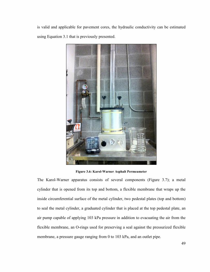
49
is valid and applicable for pavement cores, the hydraulic conductivity can be estimated
using Equation 3.1 that is previously presented.
Figure 3.6: Karol-Warner Asphalt Permeameter
The Karol-Warner apparatus consists of several components (Figure 3.7); a metal
cylinder that is opened from its top and bottom, a flexible membrane that wraps up the
inside circumferential surface of the metal cylinder, two pedestal plates (top and bottom)
to seal the metal cylinder, a graduated cylinder that is placed at the top pedestal plate, an
air pump capable of applying 103 kPa pressure in addition to evacuating the air from the
flexible membrane, an O-rings used for preserving a seal against the pressurized flexible
membrane, a pressure gauge ranging from 0 to 103 kPa, and an outlet pipe.
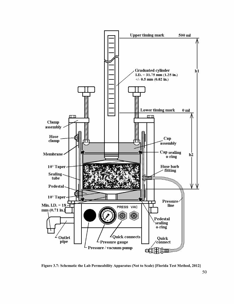
50
Figure 3.7: Schematic the Lab Permeability Apparatus (Not to Scale) [Florida Test Method, 2012]
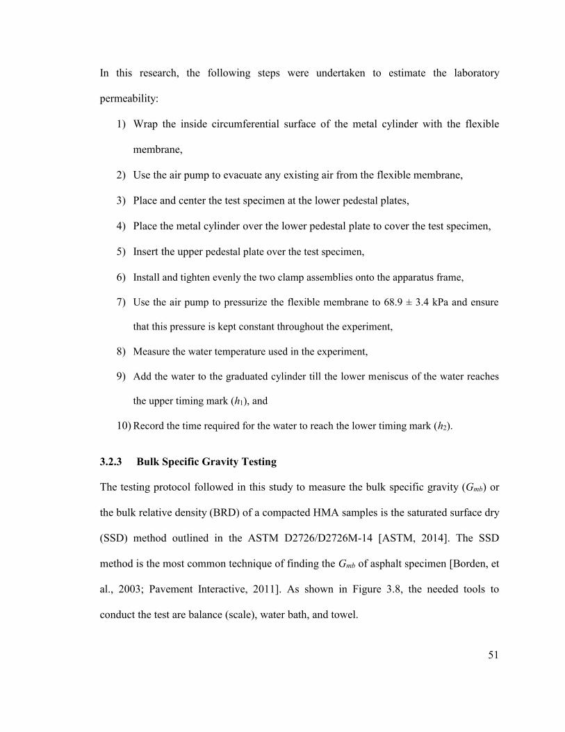
51
In this research, the following steps were undertaken to estimate the laboratory
permeability:
1) Wrap the inside circumferential surface of the metal cylinder with the flexible
membrane,
2) Use the air pump to evacuate any existing air from the flexible membrane,
3) Place and center the test specimen at the lower pedestal plates,
4) Place the metal cylinder over the lower pedestal plate to cover the test specimen,
5) Insert the upper pedestal plate over the test specimen,
6) Install and tighten evenly the two clamp assemblies onto the apparatus frame,
7) Use the air pump to pressurize the flexible membrane to 68.9 ± 3.4 kPa and ensure
that this pressure is kept constant throughout the experiment,
8) Measure the water temperature used in the experiment,
9) Add the water to the graduated cylinder till the lower meniscus of the water reaches
the upper timing mark (h1), and
10) Record the time required for the water to reach the lower timing mark (h2).
3.2.3 Bulk Specific Gravity Testing
The testing protocol followed in this study to measure the bulk specific gravity (Gmb) or
the bulk relative density (BRD) of a compacted HMA samples is the saturated surface dry
(SSD) method outlined in the ASTM D2726/D2726M-14 [ASTM, 2014]. The SSD
method is the most common technique of finding the Gmb of asphalt specimen [Borden, et
al., 2003; Pavement Interactive, 2011]. As shown in Figure 3.8, the needed tools to
conduct the test are balance (scale), water bath, and towel.
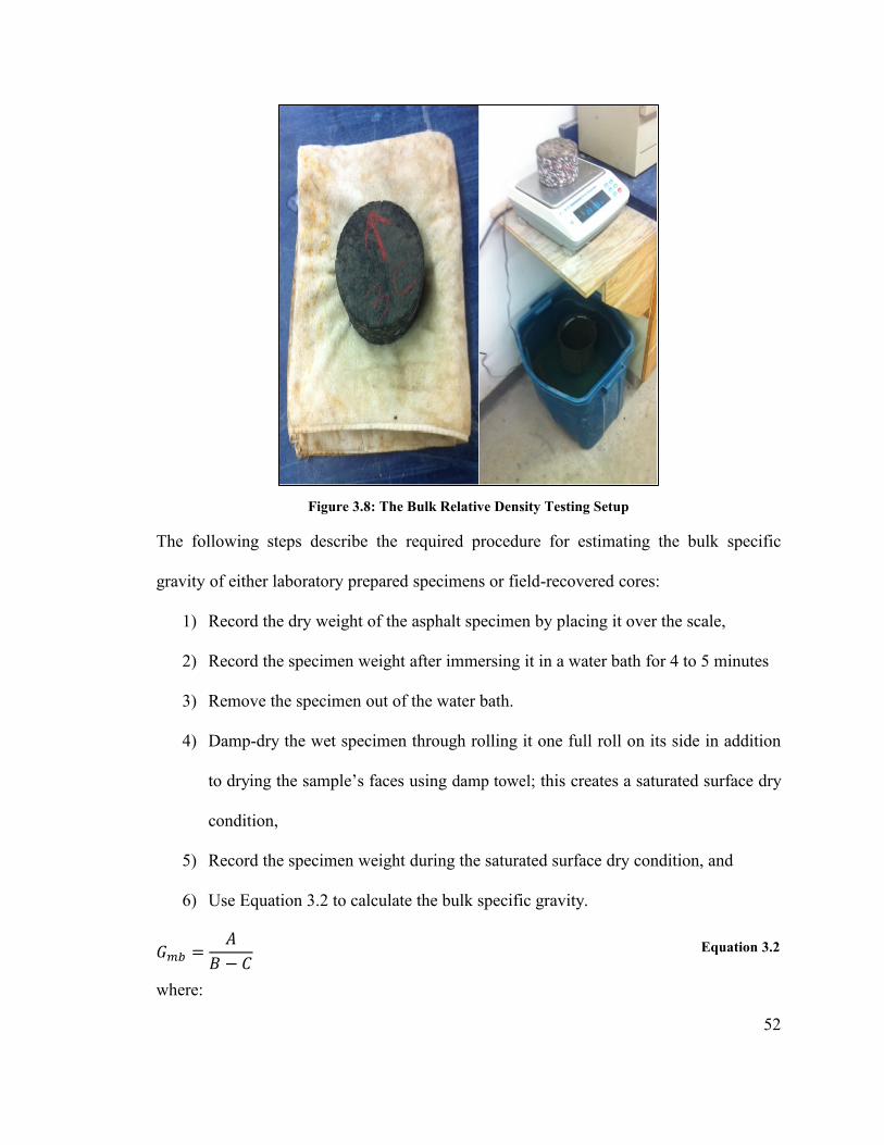
52
Figure 3.8: The Bulk Relative Density Testing Setup
The following steps describe the required procedure for estimating the bulk specific
gravity of either laboratory prepared specimens or field-recovered cores:
1) Record the dry weight of the asphalt specimen by placing it over the scale,
2) Record the specimen weight after immersing it in a water bath for 4 to 5 minutes
3) Remove the specimen out of the water bath.
4) Damp-dry the wet specimen through rolling it one full roll on its side in addition
to drying the sample’s faces using damp towel; this creates a saturated surface dry
condition,
5) Record the specimen weight during the saturated surface dry condition, and
6) Use Equation 3.2 to calculate the bulk specific gravity.
𝐺𝑚𝑏 =𝐴
𝐵 − 𝐶 Equation 3.2
where:
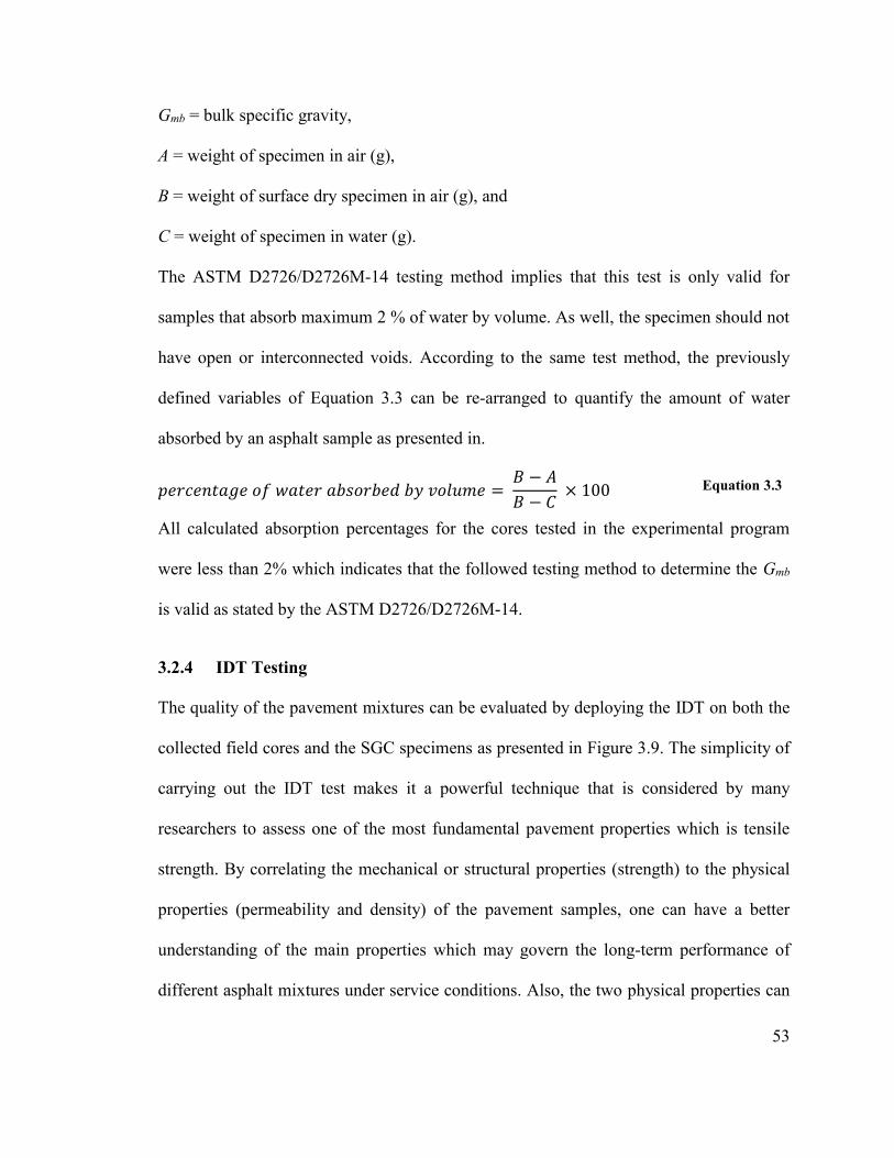
53
Gmb = bulk specific gravity,
A = weight of specimen in air (g),
B = weight of surface dry specimen in air (g), and
C = weight of specimen in water (g).
The ASTM D2726/D2726M-14 testing method implies that this test is only valid for
samples that absorb maximum 2 % of water by volume. As well, the specimen should not
have open or interconnected voids. According to the same test method, the previously
defined variables of Equation 3.3 can be re-arranged to quantify the amount of water
absorbed by an asphalt sample as presented in.
𝑝𝑒𝑟𝑐𝑒𝑛𝑡𝑎𝑔𝑒 𝑜𝑓 𝑤𝑎𝑡𝑒𝑟 𝑎𝑏𝑠𝑜𝑟𝑏𝑒𝑑 𝑏𝑦 𝑣𝑜𝑙𝑢𝑚𝑒 = 𝐵 − 𝐴
𝐵 − 𝐶 × 100 Equation 3.3
All calculated absorption percentages for the cores tested in the experimental program
were less than 2% which indicates that the followed testing method to determine the Gmb
is valid as stated by the ASTM D2726/D2726M-14.
3.2.4 IDT Testing
The quality of the pavement mixtures can be evaluated by deploying the IDT on both the
collected field cores and the SGC specimens as presented in Figure 3.9. The simplicity of
carrying out the IDT test makes it a powerful technique that is considered by many
researchers to assess one of the most fundamental pavement properties which is tensile
strength. By correlating the mechanical or structural properties (strength) to the physical
properties (permeability and density) of the pavement samples, one can have a better
understanding of the main properties which may govern the long-term performance of
different asphalt mixtures under service conditions. Also, the two physical properties can
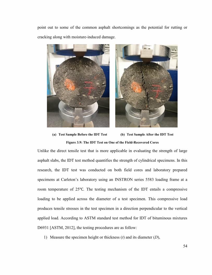
54
point out to some of the common asphalt shortcomings as the potential for rutting or
cracking along with moisture-induced damage.
(a) Test Sample Before the IDT Test (b) Test Sample After the IDT Test
Figure 3.9: The IDT Test on One of the Field-Recovered Cores
Unlike the direct tensile test that is more applicable in evaluating the strength of large
asphalt slabs, the IDT test method quantifies the strength of cylindrical specimens. In this
research, the IDT test was conducted on both field cores and laboratory prepared
specimens at Carleton’s laboratory using an INSTRON series 5583 loading frame at a
room temperature of 25℃. The testing mechanism of the IDT entails a compressive
loading to be applied across the diameter of a test specimen. This compressive load
produces tensile stresses in the test specimen in a direction perpendicular to the vertical
applied load. According to ASTM standard test method for IDT of bituminous mixtures
D6931 [ASTM, 2012], the testing procedures are as follow:
1) Measure the specimen height or thickness (t) and its diameter (D),

55
2) Place and center the specimen between the two steel strips,
3) Use the INSTRON to apply a compressive load at a rate of 50.8 mm/min,
4) Record the peak load (P) which produces a failure condition, and
5) Use Equation 3.4 to calculate the IDT of the test specimen.
𝑆𝑡 =2000 × 𝑃
𝜋 × 𝑡 × 𝐷 Equation 3.4
where:
St = IDT strength (kPa),
P = maximum load (N),
t = specimen height immediately before test (mm), and
D = specimen diameter (mm).
3.2.5 The Superpave Gyratory Compactor
The Gyratory compactor was utilized to compact the laboratory loose mix, provided by
the MTO, at different compaction levels to simulate different field densities. Before the
compaction stage using the SGC, four parameters were considered and calibrated
including the specimen height, consolidation pressure, RAM travel speed, and turntable
RPM. The calibration process was done according to the manual of operation and
instruction supplied with the SGC. Figure 3.10 shows the laboratory apparatus employed
in this research to prepare SGC specimens.
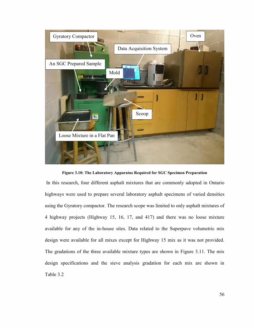
56
Figure 3.10: The Laboratory Apparatus Required for SGC Specimen Preparation
In this research, four different asphalt mixtures that are commonly adopted in Ontario
highways were used to prepare several laboratory asphalt specimens of varied densities
using the Gyratory compactor. The research scope was limited to only asphalt mixtures of
4 highway projects (Highway 15, 16, 17, and 417) and there was no loose mixture
available for any of the in-house sites. Data related to the Superpave volumetric mix
design were available for all mixes except for Highway 15 mix as it was not provided.
The gradations of the three available mixture types are shown in Figure 3.11. The mix
design specifications and the sieve analysis gradation for each mix are shown in
Table 3.2
Data Acquisition System
Gyratory Compactor
An SGC Prepared Sample
Mold
Oven
Loose Mixture in a Flat Pan
Scoop
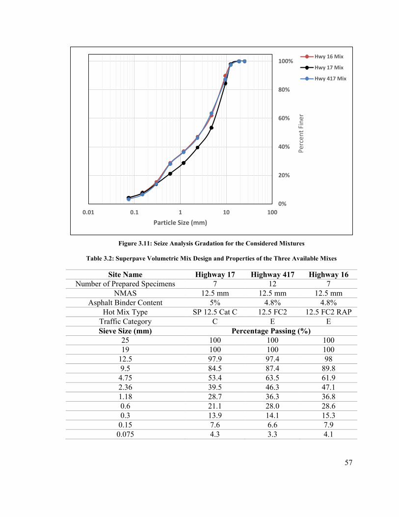
57
Figure 3.11: Seize Analysis Gradation for the Considered Mixtures
Table 3.2: Superpave Volumetric Mix Design and Properties of the Three Available Mixes
Site Name Highway 17 Highway 417 Highway 16
Number of Prepared Specimens 7 12 7
NMAS 12.5 mm 12.5 mm 12.5 mm
Asphalt Binder Content 5% 4.8% 4.8%
Hot Mix Type SP 12.5 Cat C 12.5 FC2 12.5 FC2 RAP
Traffic Category C E E
Sieve Size (mm) Percentage Passing (%)
25 100 100 100
19 100 100 100
12.5 97.9 97.4 98
9.5 84.5 87.4 89.8
4.75 53.4 63.5 61.9
2.36 39.5 46.3 47.1
1.18 28.7 36.3 36.8
0.6 21.1 28.0 28.6
0.3 13.9 14.1 15.3
0.15 7.6 6.6 7.9
0.075 4.3 3.3 4.1
0%
20%
40%
60%
80%
100%
0.01 0.1 1 10 100
Per
cen
t Fi
ner
Particle Size (mm)
Hwy 16 Mix
Hwy 17 Mix
Hwy 417 Mix
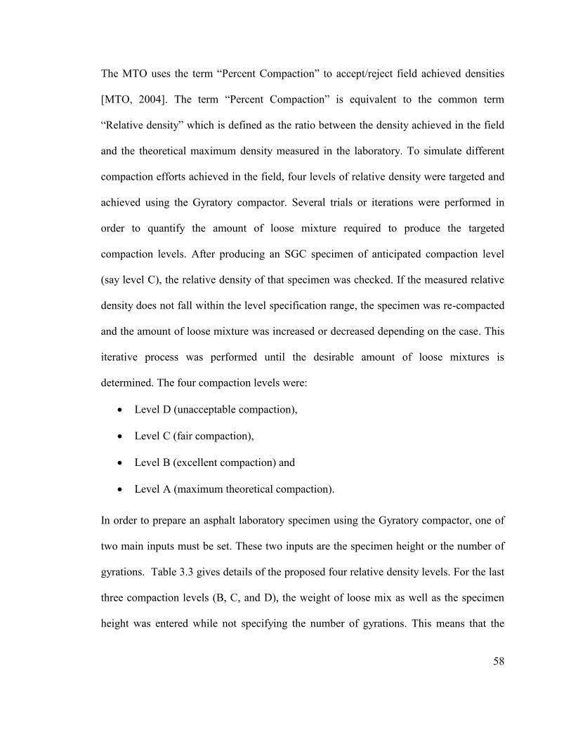
58
The MTO uses the term “Percent Compaction” to accept/reject field achieved densities
[MTO, 2004]. The term “Percent Compaction” is equivalent to the common term
“Relative density” which is defined as the ratio between the density achieved in the field
and the theoretical maximum density measured in the laboratory. To simulate different
compaction efforts achieved in the field, four levels of relative density were targeted and
achieved using the Gyratory compactor. Several trials or iterations were performed in
order to quantify the amount of loose mixture required to produce the targeted
compaction levels. After producing an SGC specimen of anticipated compaction level
(say level C), the relative density of that specimen was checked. If the measured relative
density does not fall within the level specification range, the specimen was re-compacted
and the amount of loose mixture was increased or decreased depending on the case. This
iterative process was performed until the desirable amount of loose mixtures is
determined. The four compaction levels were:
Level D (unacceptable compaction),
Level C (fair compaction),
Level B (excellent compaction) and
Level A (maximum theoretical compaction).
In order to prepare an asphalt laboratory specimen using the Gyratory compactor, one of
two main inputs must be set. These two inputs are the specimen height or the number of
gyrations. Table 3.3 gives details of the proposed four relative density levels. For the last
three compaction levels (B, C, and D), the weight of loose mix as well as the specimen
height was entered while not specifying the number of gyrations. This means that the
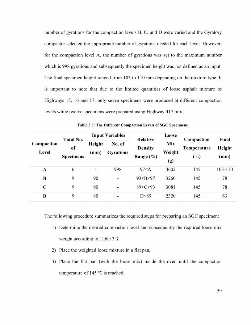
59
number of gyrations for the compaction levels B, C, and D were varied and the Gyratory
compactor selected the appropriate number of gyrations needed for each level. However,
for the compaction level A, the number of gyrations was set to the maximum number
which is 998 gyrations and subsequently the specimen height was not defined as an input.
The final specimen height ranged from 103 to 110 mm depending on the mixture type. It
is important to note that due to the limited quantities of loose asphalt mixture of
Highways 15, 16 and 17, only seven specimens were produced at different compaction
levels while twelve specimens were prepared using Highway 417 mix.
Table 3.3: The Different Compaction Levels of SGC Specimens.
Compaction
Level
Total No.
of
Specimens
Input Variables Relative
Density
Range (%)
Loose
Mix
Weight
(g)
Compaction
Temperature
(℃)
Final
Height
(mm)
Height
(mm)
No. of
Gyrations
A 6 - 998 97<A 4602 145 103-110
B 9 90 - 93<B<97 3260 145 78
C 9 90 - 89<C<93 3081 145 78
D 9 80 - D<89 2320 145 63
The following procedure summarizes the required steps for preparing an SGC specimen:
1) Determine the desired compaction level and subsequently the required loose mix
weight according to Table 3.3,
2) Place the weighted loose mixture in a flat pan,
3) Place the flat pan (with the loose mix) inside the oven until the compaction
temperature of 145 ℃ is reached,
60
4) Place the compaction mold, the bottom and top base plate inside the oven 30 to 45
minutes prior to the compaction process at temperature close to the compaction
temperature (150 ℃ was used in this research). This is necessary to prevent heat
loss due to the possible difference in temperatures between the mold and the
heated mix.
5) Carefully remove the pre-heated mold and plates from the oven,
6) Place bottom base plate and a paper disc at the mold’s bottom,
7) Use a scoop to carefully place the heated mixture into the mold,
8) Level the mixture evenly,
9) Add another paper disc and the top base plate on the leveled surface of the
mixture,
10) Place the mold inside the Gyratory compactor and center it under the loading ram,
11) Define the input parameter (the targeted height or the number of gyrations),
12) Input the consolidation pressure as 600 kPa, the angular velocity as 30
gyrations/min, and the gyratory angle as 1.25° into the connected data acquisition
system,
13) Start the compaction process, and
14) Remove the SGC sample from the Gyratory compactor and let it cool at the room
temperature (25°C).

61
For each prepared specimen of each mixture, the density, laboratory permeability, and
IDT were determined using the laboratory test methods discussed earlier. Firstly, the bulk
relative density test was performed for all prepared samples followed by the laboratory
measurement of their permeability, and finally the determination of the IDT.
3.3 Summary
In summary, this chapter presented the experimental program followed to accomplish the
research objectives. The testing program included field and laboratory investigations of
newly and in-service roads finished by two distinctly different compaction methods. The
next chapter will present the results of the field and laboratory carried investigations.
62
CHAPTER 4: RESULTS OF THE
EXPERIMENTAL PROGRAM
The previous chapter explained the testing program including explanations of the
conducted experiments in two different settings; the field and laboratory. This chapter
presents the results obtained from both the field and laboratory investigations. The
chapter consists of two main sections. The first section provides results of the measured
permeability values in the field, the second section deals with presenting the laboratory
investigations incorporating both the measurements and results of the SGC specimens as
well as the results of the laboratory testing on the collected field cores.
4.1 Field Investigations
This section of the chapter is devoted to display the field investigation test results of nine
inspected sites, which included seven highway projects and two in-house asphalt
pavement projects in Ontario. The in-situ field investigations were initiated during the
summer of 2012 and continued until the late fall of 2014.
Table 4.1 summarizes all sites examined in this study, the compaction method used at
each site, and the implemented type of investigation. In total, five (out of the total of
nine) sites are common projects where the two compaction techniques were used. The
field results obtained by the two different compaction techniques are present in this
section. Firstly, the field results of various sites paved and compacted by the conventional
vibratory steel drum and pneumatic train rollers are illustrated. Secondly, the results of
field investigations on sites compacted by the AMIR-II roller are presented for the
purpose of comparison.
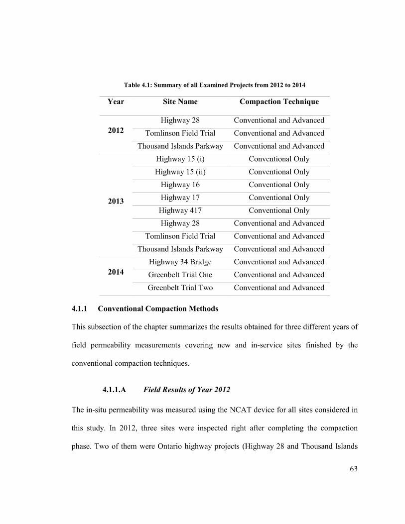
63
Table 4.1: Summary of all Examined Projects from 2012 to 2014
Year Site Name Compaction Technique
2012
Highway 28 Conventional and Advanced
Tomlinson Field Trial Conventional and Advanced
Thousand Islands Parkway Conventional and Advanced
2013
Highway 15 (i) Conventional Only
Highway 15 (ii) Conventional Only
Highway 16 Conventional Only
Highway 17 Conventional Only
Highway 417 Conventional Only
Highway 28 Conventional and Advanced
Tomlinson Field Trial Conventional and Advanced
Thousand Islands Parkway Conventional and Advanced
2014
Highway 34 Bridge Conventional and Advanced
Greenbelt Trial One Conventional and Advanced
Greenbelt Trial Two Conventional and Advanced
4.1.1 Conventional Compaction Methods
This subsection of the chapter summarizes the results obtained for three different years of
field permeability measurements covering new and in-service sites finished by the
conventional compaction techniques.
4.1.1.A Field Results of Year 2012
The in-situ permeability was measured using the NCAT device for all sites considered in
this study. In 2012, three sites were inspected right after completing the compaction
phase. Two of them were Ontario highway projects (Highway 28 and Thousand Islands
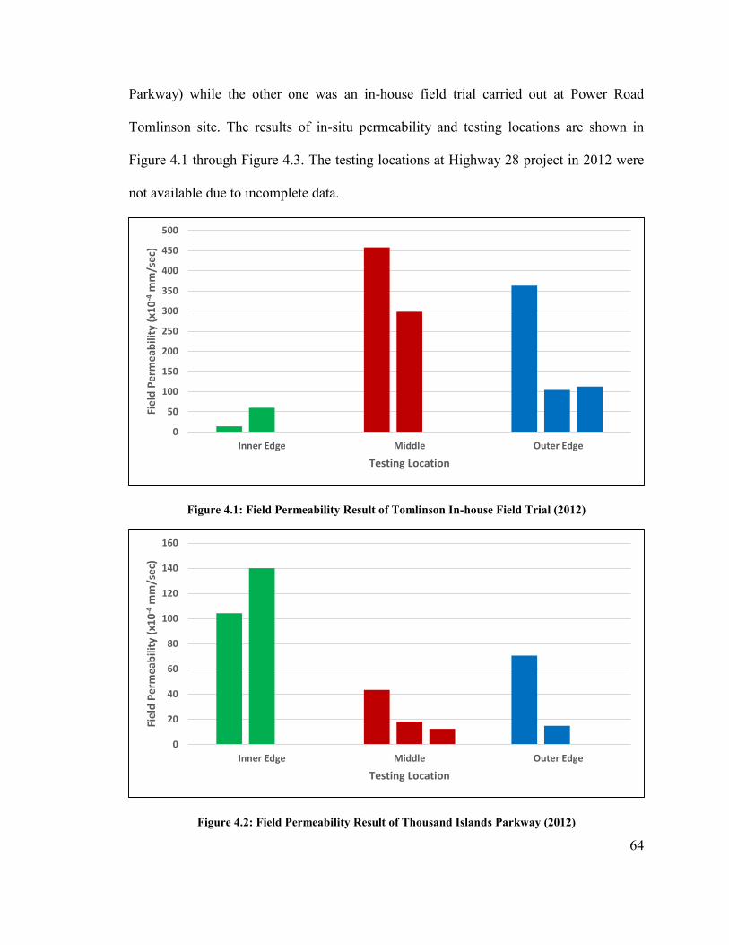
64
Parkway) while the other one was an in-house field trial carried out at Power Road
Tomlinson site. The results of in-situ permeability and testing locations are shown in
Figure 4.1 through Figure 4.3. The testing locations at Highway 28 project in 2012 were
not available due to incomplete data.
Figure 4.1: Field Permeability Result of Tomlinson In-house Field Trial (2012)
Figure 4.2: Field Permeability Result of Thousand Islands Parkway (2012)
0
50
100
150
200
250
300
350
400
450
500
Inner Edge Middle Outer Edge
Fie
ld P
erm
eab
ility
(x1
0-4
mm
/se
c)
Testing Location
0
20
40
60
80
100
120
140
160
Inner Edge Middle Outer Edge
Fie
ld P
erm
eab
ility
(x1
0-4
mm
/se
c)
Testing Location
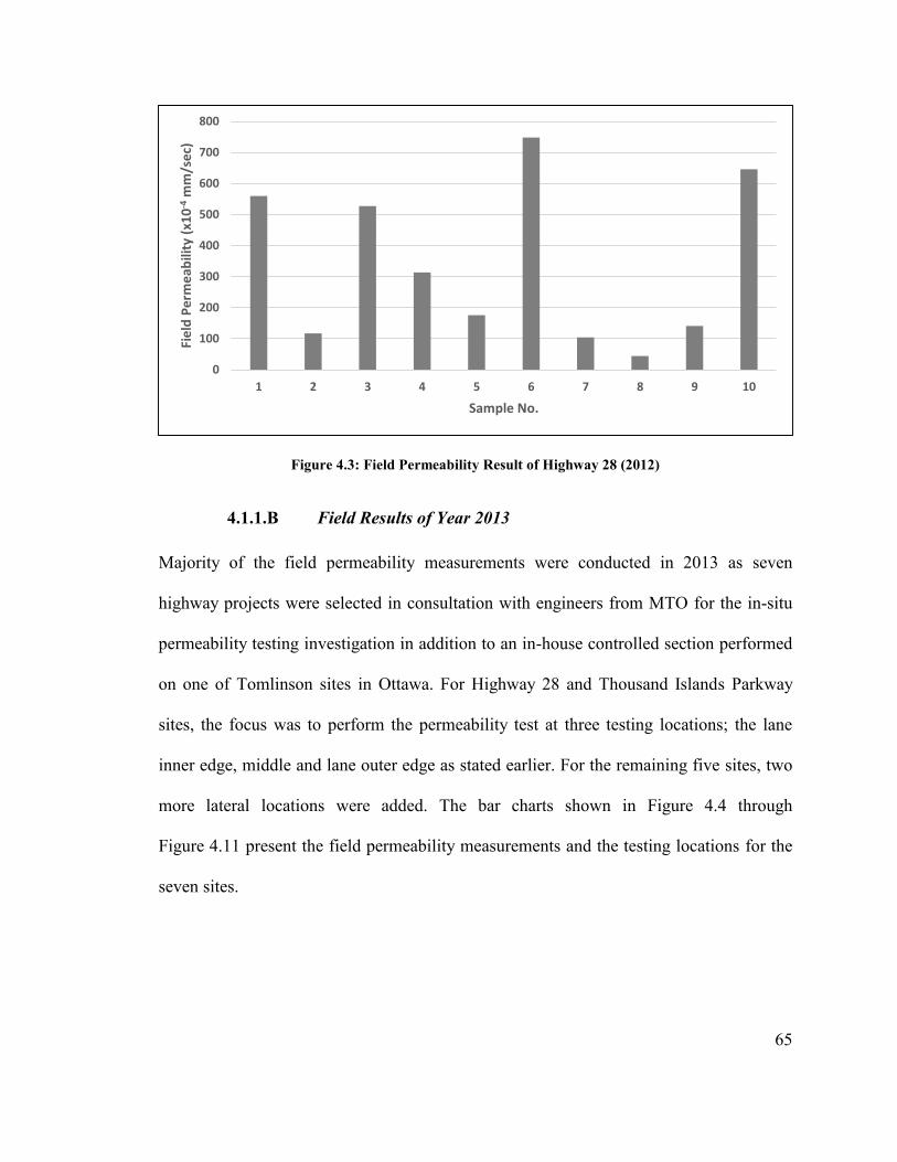
65
Figure 4.3: Field Permeability Result of Highway 28 (2012)
4.1.1.B Field Results of Year 2013
Majority of the field permeability measurements were conducted in 2013 as seven
highway projects were selected in consultation with engineers from MTO for the in-situ
permeability testing investigation in addition to an in-house controlled section performed
on one of Tomlinson sites in Ottawa. For Highway 28 and Thousand Islands Parkway
sites, the focus was to perform the permeability test at three testing locations; the lane
inner edge, middle and lane outer edge as stated earlier. For the remaining five sites, two
more lateral locations were added. The bar charts shown in Figure 4.4 through
Figure 4.11 present the field permeability measurements and the testing locations for the
seven sites.
0
100
200
300
400
500
600
700
800
1 2 3 4 5 6 7 8 9 10
Fie
ld P
erm
eab
ility
(x1
0-4
mm
/se
c)
Sample No.
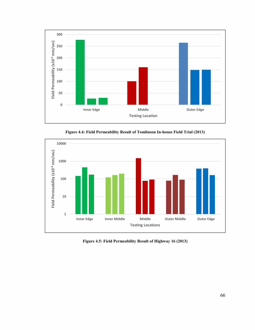
66
Figure 4.4: Field Permeability Result of Tomlinson In-house Field Trial (2013)
Figure 4.5: Field Permeability Result of Highway 16 (2013)
0
50
100
150
200
250
300
Inner Edge Middle Outer Edge
Fie
ld P
erm
eab
ility
(x1
0-4
mm
/se
c)
Testing Location
1
10
100
1000
10000
Inner Edge Inner Middle Middle Outer Middle Outer Edge
Fie
ld P
erm
eab
ility
(x1
0-4
mm
/se
c)
Testing Locations

67
Figure 4.6: Field Permeability Result of Highway 17 (2013)
Figure 4.7: Field Permeability Result of Highway 417 (2013)
0
100
200
300
400
500
600
Inner Edge Inner Middle Middle Outer Middle Outer Edge
Fie
ld P
erm
eab
ility
(x1
0-4
mm
/se
c)
Testing Locations
1
10
100
1000
10000
Inner Edge Inner Middle Middle Outer Middle Outer Edge
Fie
ld P
erm
eab
ility
(x1
0-4
mm
/se
c)
Testing Locations
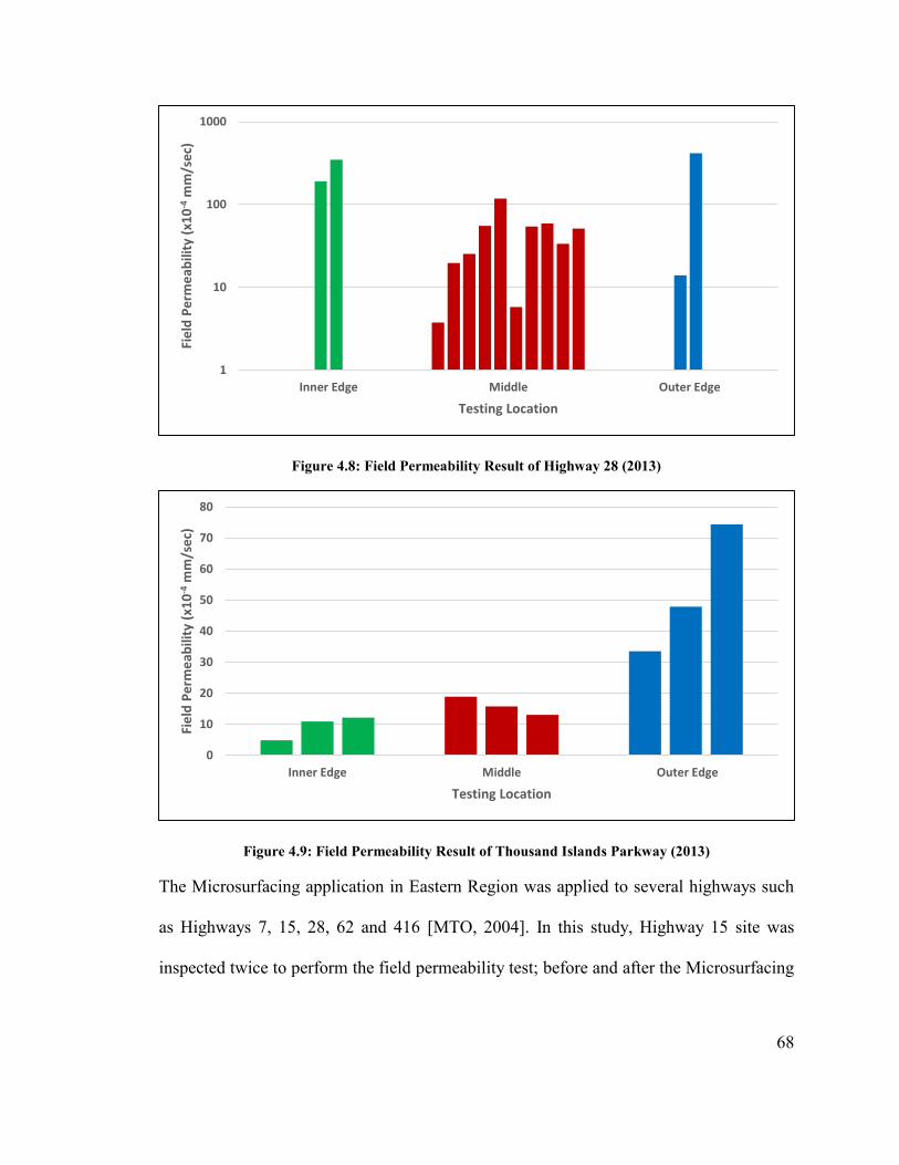
68
Figure 4.8: Field Permeability Result of Highway 28 (2013)
Figure 4.9: Field Permeability Result of Thousand Islands Parkway (2013)
The Microsurfacing application in Eastern Region was applied to several highways such
as Highways 7, 15, 28, 62 and 416 [MTO, 2004]. In this study, Highway 15 site was
inspected twice to perform the field permeability test; before and after the Microsurfacing
1
10
100
1000
Inner Edge Middle Outer Edge
Fie
ld P
erm
eab
ility
(x1
0-4
mm
/se
c)
Testing Location
0
10
20
30
40
50
60
70
80
Inner Edge Middle Outer Edge
Fie
ld P
erm
eab
ility
(x1
0-4
mm
/se
c)
Testing Location
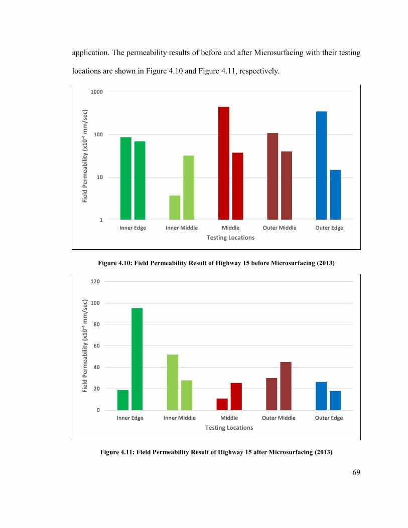
69
application. The permeability results of before and after Microsurfacing with their testing
locations are shown in Figure 4.10 and Figure 4.11, respectively.
Figure 4.10: Field Permeability Result of Highway 15 before Microsurfacing (2013)
Figure 4.11: Field Permeability Result of Highway 15 after Microsurfacing (2013)
1
10
100
1000
Inner Edge Inner Middle Middle Outer Middle Outer Edge
Fie
ld P
erm
eab
ility
(x1
0-4
mm
/se
c)
Testing Locations
0
20
40
60
80
100
120
Inner Edge Inner Middle Middle Outer Middle Outer Edge
Fie
ld P
erm
eab
ility
(x1
0-4
mm
/se
c)
Testing Locations
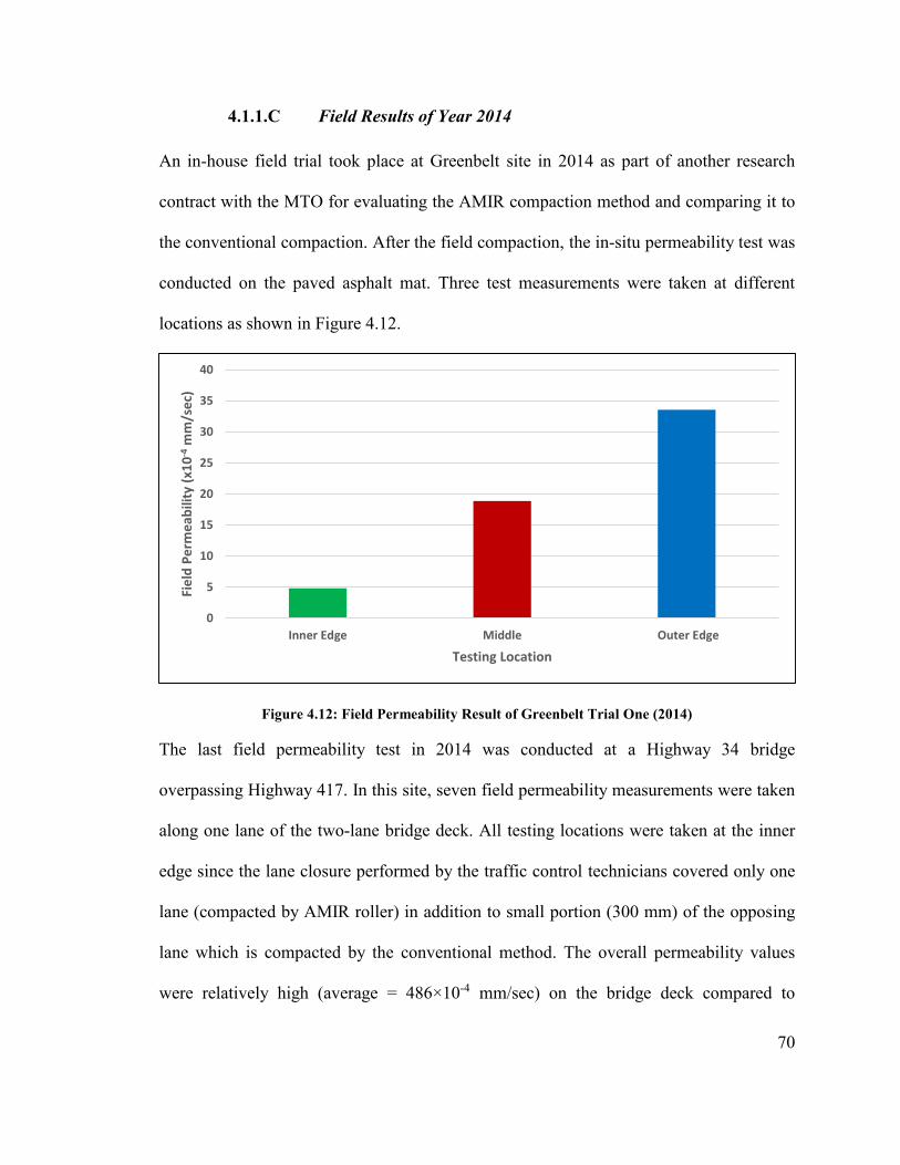
70
4.1.1.C Field Results of Year 2014
An in-house field trial took place at Greenbelt site in 2014 as part of another research
contract with the MTO for evaluating the AMIR compaction method and comparing it to
the conventional compaction. After the field compaction, the in-situ permeability test was
conducted on the paved asphalt mat. Three test measurements were taken at different
locations as shown in Figure 4.12.
Figure 4.12: Field Permeability Result of Greenbelt Trial One (2014)
The last field permeability test in 2014 was conducted at a Highway 34 bridge
overpassing Highway 417. In this site, seven field permeability measurements were taken
along one lane of the two-lane bridge deck. All testing locations were taken at the inner
edge since the lane closure performed by the traffic control technicians covered only one
lane (compacted by AMIR roller) in addition to small portion (300 mm) of the opposing
lane which is compacted by the conventional method. The overall permeability values
were relatively high (average = 486×10-4 mm/sec) on the bridge deck compared to
0
5
10
15
20
25
30
35
40
Inner Edge Middle Outer Edge
Fie
ld P
erm
eab
ility
(x1
0-4
mm
/se
c)
Testing Location
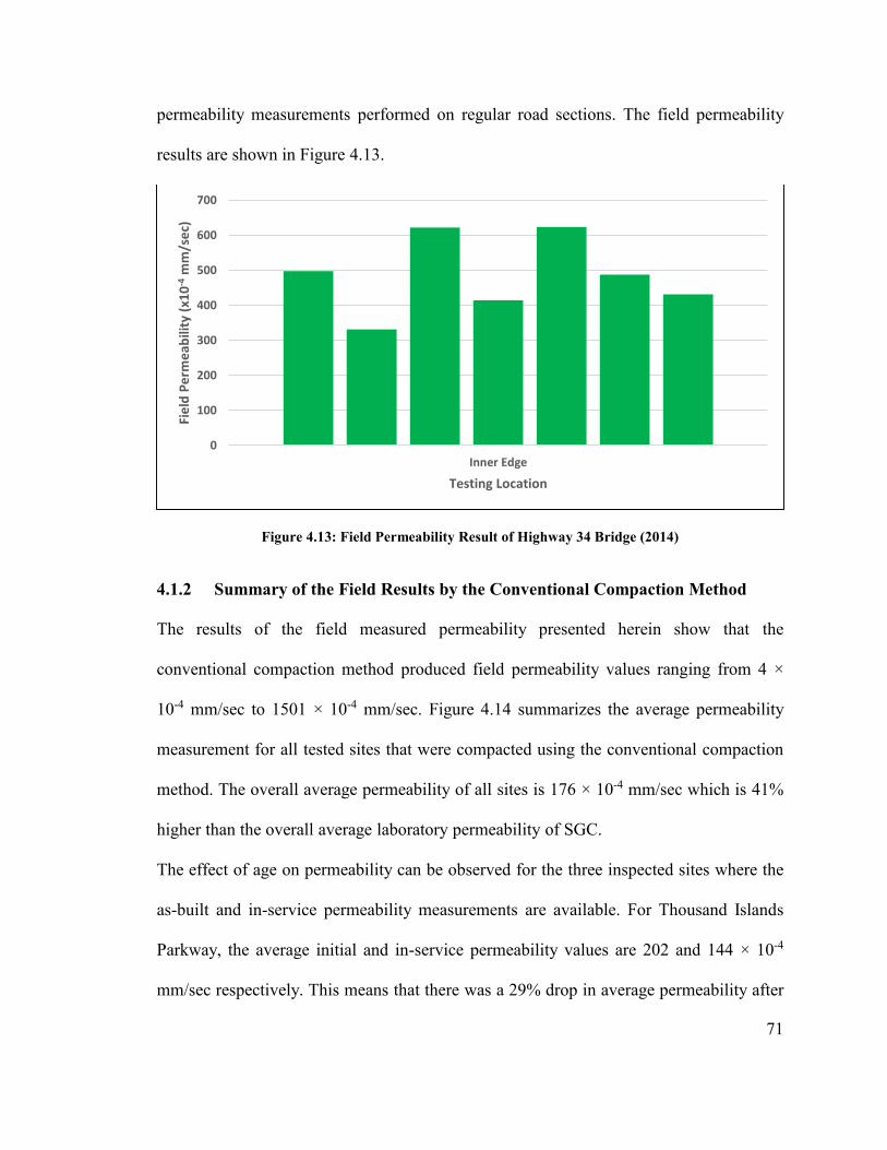
71
permeability measurements performed on regular road sections. The field permeability
results are shown in Figure 4.13.
Figure 4.13: Field Permeability Result of Highway 34 Bridge (2014)
4.1.2 Summary of the Field Results by the Conventional Compaction Method
The results of the field measured permeability presented herein show that the
conventional compaction method produced field permeability values ranging from 4 ×
10-4 mm/sec to 1501 × 10-4 mm/sec. Figure 4.14 summarizes the average permeability
measurement for all tested sites that were compacted using the conventional compaction
method. The overall average permeability of all sites is 176 × 10-4 mm/sec which is 41%
higher than the overall average laboratory permeability of SGC.
The effect of age on permeability can be observed for the three inspected sites where the
as-built and in-service permeability measurements are available. For Thousand Islands
Parkway, the average initial and in-service permeability values are 202 and 144 × 10-4
mm/sec respectively. This means that there was a 29% drop in average permeability after
0
100
200
300
400
500
600
700
Inner Edge
Fie
ld P
erm
eab
ility
(x1
0-4
mm
/se
c)
Testing Location
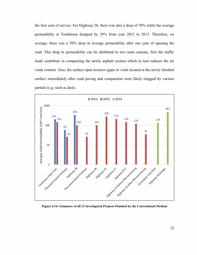
72
the first year of service. For Highway 28, there was also a drop of 70% while the average
permeability at Tomlinson dropped by 29% from year 2012 to 2013. Therefore, on
average, there was a 50% drop in average permeability after one year of opening the
road. This drop in permeability can be attributed to two main reasons, first the traffic
loads contribute in compacting the newly asphalt section which in turn reduces the air
voids content. Also, the surface open textures (gaps or voids located at the newly finished
surface immediately after road paving and compaction were likely clogged by various
partials (e.g. such as dust).
Figure 4.14: Summary of all 12 Investigated Projects Finished by the Conventional Method
202
58
338
145
26
100
26
100
280214
146120
35
134
487
1
10
100
1000
Ave
rgae
Fie
ld P
erm
eab
ility
(x1
0-4
mm
/se
c)
2012 2013 2014
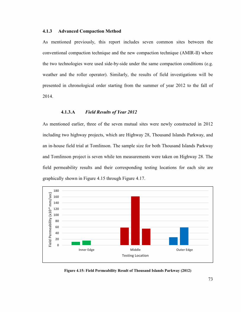
73
4.1.3 Advanced Compaction Method
As mentioned previously, this report includes seven common sites between the
conventional compaction technique and the new compaction technique (AMIR-II) where
the two technologies were used side-by-side under the same compaction conditions (e.g.
weather and the roller operator). Similarly, the results of field investigations will be
presented in chronological order starting from the summer of year 2012 to the fall of
2014.
4.1.3.A Field Results of Year 2012
As mentioned earlier, three of the seven mutual sites were newly constructed in 2012
including two highway projects, which are Highway 28, Thousand Islands Parkway, and
an in-house field trial at Tomlinson. The sample size for both Thousand Islands Parkway
and Tomlinson project is seven while ten measurements were taken on Highway 28. The
field permeability results and their corresponding testing locations for each site are
graphically shown in Figure 4.15 through Figure 4.17.
Figure 4.15: Field Permeability Result of Thousand Islands Parkway (2012)
0
20
40
60
80
100
120
140
160
180
Inner Edge Middle Outer Edge
Fie
ld P
erm
eab
ility
(x1
0-4
mm
/se
c)
Testing Location
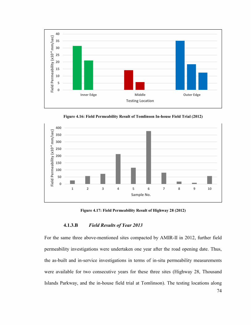
74
Figure 4.16: Field Permeability Result of Tomlinson In-house Field Trial (2012)
Figure 4.17: Field Permeability Result of Highway 28 (2012)
4.1.3.B Field Results of Year 2013
For the same three above-mentioned sites compacted by AMIR-II in 2012, further field
permeability investigations were undertaken one year after the road opening date. Thus,
the as-built and in-service investigations in terms of in-situ permeability measurements
were available for two consecutive years for these three sites (Highway 28, Thousand
Islands Parkway, and the in-house field trial at Tomlinson). The testing locations along
0
5
10
15
20
25
30
35
40
Inner Edge Middle Outer Edge
Fie
ld P
erm
eab
ility
(x1
0-4
mm
/se
c)
Testing Location
0
50
100
150
200
250
300
350
400
1 2 3 4 5 6 7 8 9 10
Fie
ld P
erm
eab
ility
(x1
0-4
mm
/se
c)
Sample No.
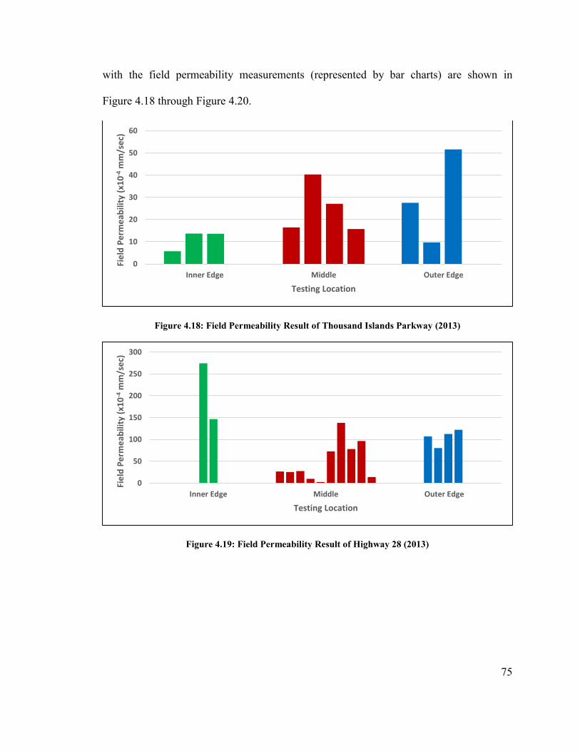
75
with the field permeability measurements (represented by bar charts) are shown in
Figure 4.18 through Figure 4.20.
Figure 4.18: Field Permeability Result of Thousand Islands Parkway (2013)
Figure 4.19: Field Permeability Result of Highway 28 (2013)
0
10
20
30
40
50
60
Inner Edge Middle Outer Edge
Fie
ld P
erm
eab
ility
(x1
0-4
mm
/se
c)
Testing Location
0
50
100
150
200
250
300
Inner Edge Middle Outer Edge
Fie
ld P
erm
eab
ility
(x1
0-4
mm
/se
c)
Testing Location
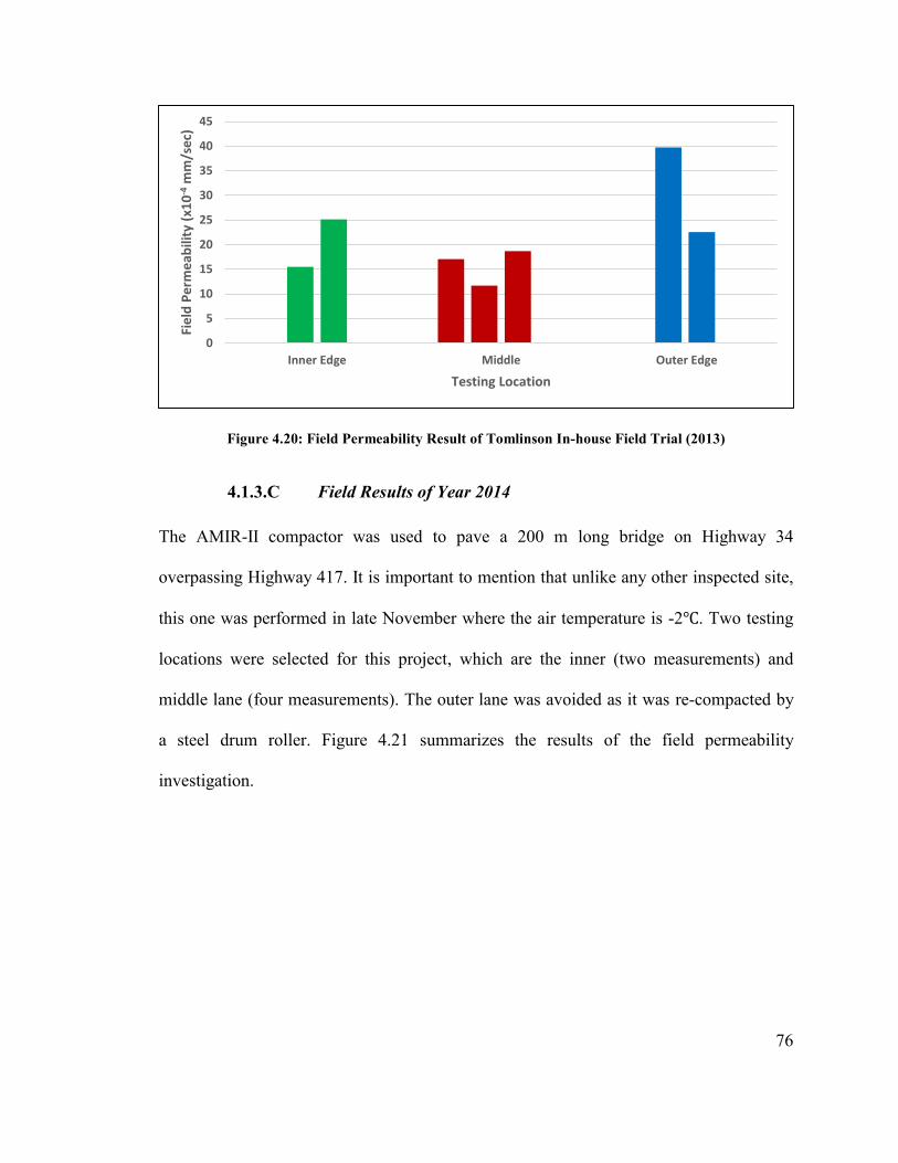
76
Figure 4.20: Field Permeability Result of Tomlinson In-house Field Trial (2013)
4.1.3.C Field Results of Year 2014
The AMIR-II compactor was used to pave a 200 m long bridge on Highway 34
overpassing Highway 417. It is important to mention that unlike any other inspected site,
this one was performed in late November where the air temperature is -2℃. Two testing
locations were selected for this project, which are the inner (two measurements) and
middle lane (four measurements). The outer lane was avoided as it was re-compacted by
a steel drum roller. Figure 4.21 summarizes the results of the field permeability
investigation.
0
5
10
15
20
25
30
35
40
45
Inner Edge Middle Outer Edge
Fie
ld P
erm
eab
ility
(x1
0-4
mm
/se
c)
Testing Location
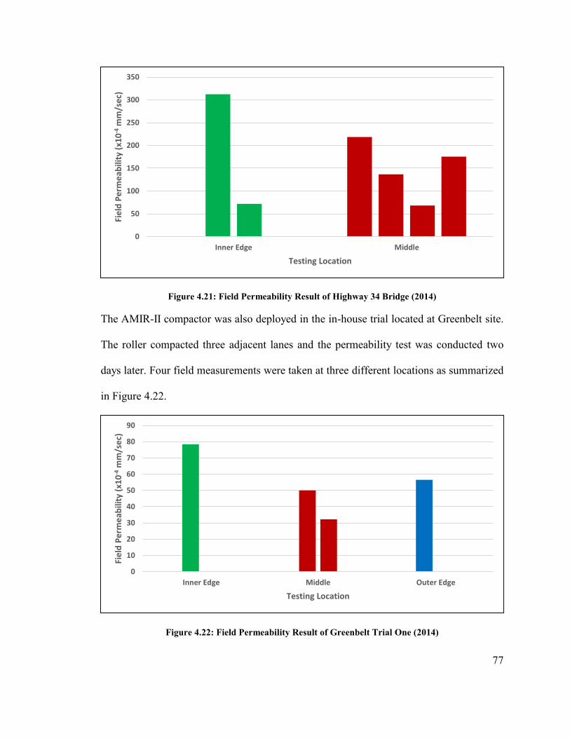
77
Figure 4.21: Field Permeability Result of Highway 34 Bridge (2014)
The AMIR-II compactor was also deployed in the in-house trial located at Greenbelt site.
The roller compacted three adjacent lanes and the permeability test was conducted two
days later. Four field measurements were taken at three different locations as summarized
in Figure 4.22.
Figure 4.22: Field Permeability Result of Greenbelt Trial One (2014)
0
50
100
150
200
250
300
350
Inner Edge Middle
Fie
ld P
erm
eab
ility
(x1
0-4
mm
/se
c)
Testing Location
0
10
20
30
40
50
60
70
80
90
Inner Edge Middle Outer Edge
Fie
ld P
erm
eab
ility
(x1
0-4
mm
/se
c)
Testing Location
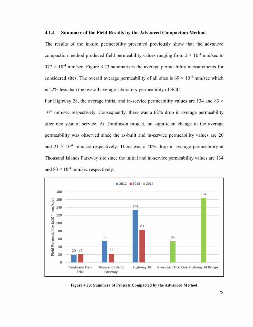
78
4.1.4 Summary of the Field Results by the Advanced Compaction Method
The results of the in-situ permeability presented previously show that the advanced
compaction method produced field permeability values ranging from 2 × 10⁻⁴ mm/sec to
377 × 10-4 mm/sec. Figure 4.23 summarizes the average permeability measurements for
considered sites. The overall average permeability of all sites is 69 × 10-4 mm/sec which
is 22% less than the overall average laboratory permeability of SGC.
For Highway 28, the average initial and in-service permeability values are 134 and 83 ×
10-4 mm/sec respectively. Consequently, there was a 62% drop in average permeability
after one year of service. At Tomlinson project, no significant change in the average
permeability was observed since the as-built and in-service permeability values are 20
and 21 × 10-4 mm/sec respectively. There was a 40% drop in average permeability at
Thousand Islands Parkway site since the initial and in-service permeability values are 134
and 83 × 10-4 mm/sec respectively.
Figure 4.23: Summary of Projects Compacted by the Advanced Method
20
55
134
21 22
83
54
164
0
20
40
60
80
100
120
140
160
180
Tomlinson FieldTrial
Thousand IslandParkway
Highway 28 Greenbelt Trial One Highway 34 Bridge
Fie
ld P
erm
eab
ility
(x1
0-4
mm
/se
c)
2012 2013 2014
79
4.2 Laboratory Investigations
The second section of this chapter presents the laboratory results of both the SGC
specimens and field cores. The laboratory phase incorporated cores recovered from eight
sites; six highway projects and two in-house field trials. The total number of common
sites between the two compaction methods is four. This section presents first the results
produced by the SGC specimens followed by the field-recovered cores.
4.2.1 Results of Superpave Gyratory Compactor Specimens
In total, the gyratory compactor was used to prepare 33 specimens of different
engineering properties. Table 4.2 presents the test results for each mix under the four
compaction levels introduced in the previous chapter. In order to illustrate the laboratory
results graphically, the average bulk specific gravity, IDT, and permeability of each
compaction level are plotted in Figure 4.24 through Figure 4.26. In general, the results
show that as the achieved relative density increases, the IDT increases while the
permeability. These results are observed for all four highway asphalt mixtures.
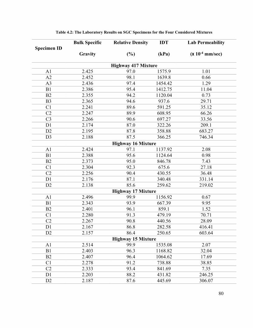
80
Table 4.2: The Laboratory Results on SGC Specimens for the Four Considered Mixtures
Specimen ID
Bulk Specific
Gravity
Relative Density
(%)
IDT
(kPa)
Lab Permeability
(x 10-4 mm/sec)
Highway 417 Mixture
A1 2.425 97.0 1575.9 1.01
A2 2.452 98.1 1639.8 0.66
A3 2.436 97.4 1454.42 1.29
B1 2.386 95.4 1412.75 11.04
B2 2.355 94.2 1120.04 0.73
B3 2.365 94.6 937.6 29.71
C1 2.241 89.6 591.25 35.12
C2 2.247 89.9 608.95 66.26
C3 2.266 90.6 697.27 33.56
D1 2.174 87.0 322.26 209.1
D2 2.195 87.8 358.88 683.27
D3 2.188 87.5 366.25 746.34
Highway 16 Mixture
A1 2.424 97.1 1137.92 2.08
B1 2.388 95.6 1124.64 0.98
B2 2.373 95.0 846.78 7.43
C1 2.304 92.3 675.6 27.18
C2 2.256 90.4 430.55 36.48
D1 2.176 87.1 340.48 331.14
D2 2.138 85.6 259.62 219.02
Highway 17 Mixture
A1 2.496 99.9 1156.92 0.67
B1 2.343 93.9 667.39 9.95
B2 2.401 96.1 859.1 1.52
C1 2.280 91.3 479.19 70.71
C2 2.267 90.8 440.56 28.09
D1 2.167 86.8 282.58 416.41
D2 2.157 86.4 250.65 603.64
Highway 15 Mixture
A1 2.514 99.9 1535.08 2.07
B1 2.403 96.3 1168.82 32.04
B2 2.407 96.4 1064.62 17.69
C1 2.278 91.2 738.88 38.85
C2 2.333 93.4 841.69 7.35
D1 2.203 88.2 431.82 246.25
D2 2.187 87.6 445.69 306.07
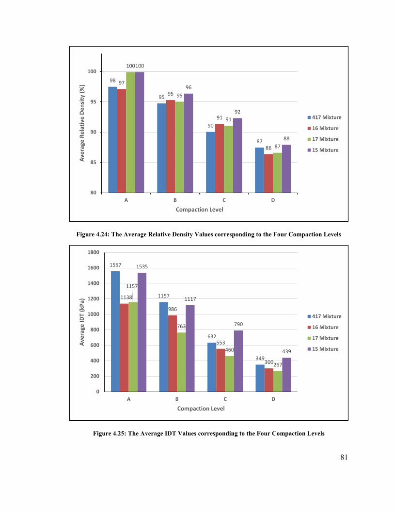
81
Figure 4.24: The Average Relative Density Values corresponding to the Four Compaction Levels
Figure 4.25: The Average IDT Values corresponding to the Four Compaction Levels
98
95
90
87
97
95
91
86
100
95
91
87
100
96
92
88
80
85
90
95
100
A B C D
Ave
rage
Re
lati
ve D
en
sity
(%
)
Compaction Level
417 Mixture
16 Mixture
17 Mixture
15 Mixture
1557
1157
632
349
1138
986
553
300
1157
763
460
267
1535
1117
790
439
0
200
400
600
800
1000
1200
1400
1600
1800
A B C D
Ave
rage
ID
T (k
Pa)
Compaction Level
417 Mixture
16 Mixture
17 Mixture
15 Mixture
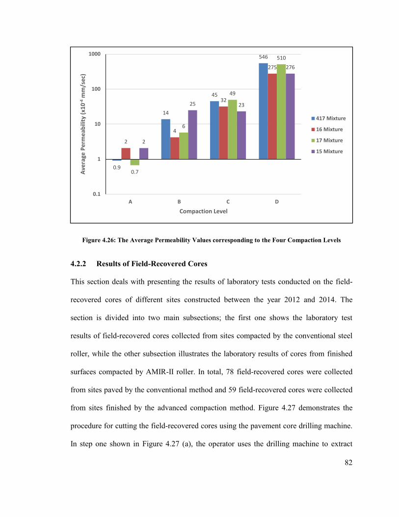
82
Figure 4.26: The Average Permeability Values corresponding to the Four Compaction Levels
4.2.2 Results of Field-Recovered Cores
This section deals with presenting the results of laboratory tests conducted on the field-
recovered cores of different sites constructed between the year 2012 and 2014. The
section is divided into two main subsections; the first one shows the laboratory test
results of field-recovered cores collected from sites compacted by the conventional steel
roller, while the other subsection illustrates the laboratory results of cores from finished
surfaces compacted by AMIR-II roller. In total, 78 field-recovered cores were collected
from sites paved by the conventional method and 59 field-recovered cores were collected
from sites finished by the advanced compaction method. Figure 4.27 demonstrates the
procedure for cutting the field-recovered cores using the pavement core drilling machine.
In step one shown in Figure 4.27 (a), the operator uses the drilling machine to extract
0.9
14
45
546
2
4
32
275
0.7
6
49
510
2
25 23
276
0.1
1
10
100
1000
A B C D
Ave
rage
Pe
rme
abili
ty (
x10
-4m
m/s
ec)
Compaction Level
417 Mixture
16 Mixture
17 Mixture
15 Mixture
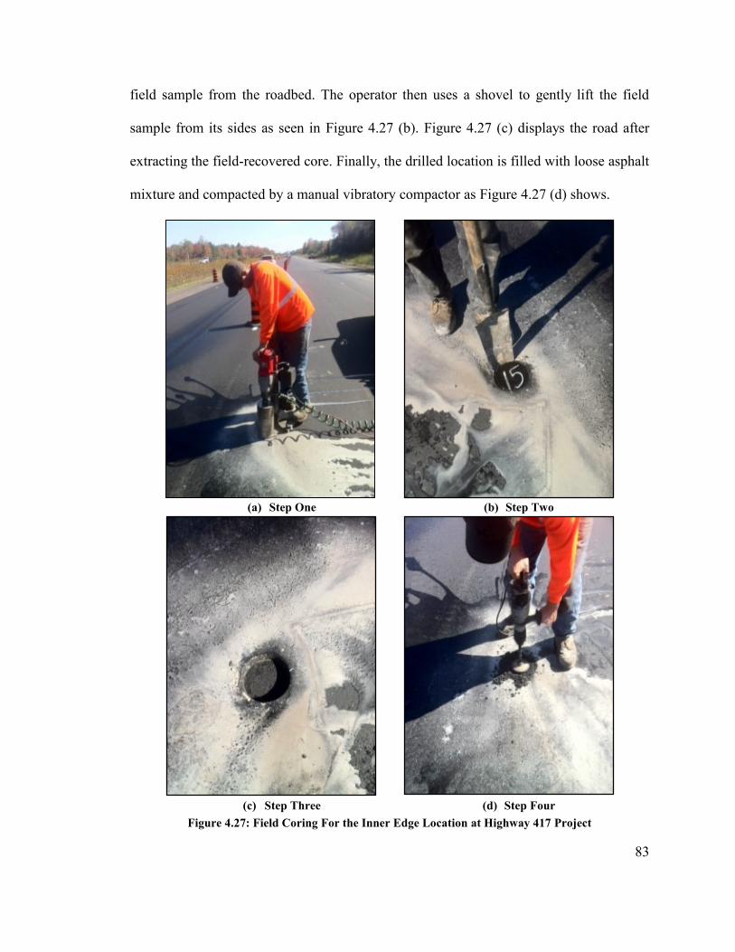
83
field sample from the roadbed. The operator then uses a shovel to gently lift the field
sample from its sides as seen in Figure 4.27 (b). Figure 4.27 (c) displays the road after
extracting the field-recovered core. Finally, the drilled location is filled with loose asphalt
mixture and compacted by a manual vibratory compactor as Figure 4.27 (d) shows.
(a) Step One (b) Step Two
(c) Step Three (d) Step Four
Figure 4.27: Field Coring For the Inner Edge Location at Highway 417 Project
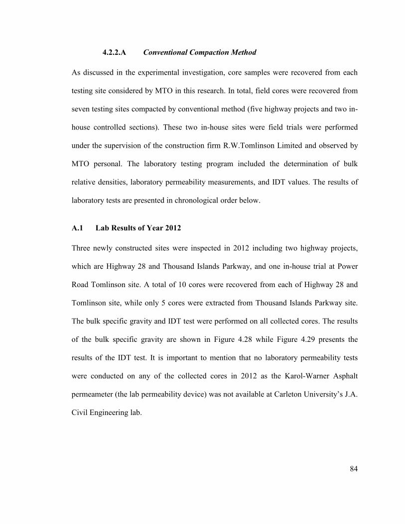
84
4.2.2.A Conventional Compaction Method
As discussed in the experimental investigation, core samples were recovered from each
testing site considered by MTO in this research. In total, field cores were recovered from
seven testing sites compacted by conventional method (five highway projects and two in-
house controlled sections). These two in-house sites were field trials were performed
under the supervision of the construction firm R.W.Tomlinson Limited and observed by
MTO personal. The laboratory testing program included the determination of bulk
relative densities, laboratory permeability measurements, and IDT values. The results of
laboratory tests are presented in chronological order below.
A.1 Lab Results of Year 2012
Three newly constructed sites were inspected in 2012 including two highway projects,
which are Highway 28 and Thousand Islands Parkway, and one in-house trial at Power
Road Tomlinson site. A total of 10 cores were recovered from each of Highway 28 and
Tomlinson site, while only 5 cores were extracted from Thousand Islands Parkway site.
The bulk specific gravity and IDT test were performed on all collected cores. The results
of the bulk specific gravity are shown in Figure 4.28 while Figure 4.29 presents the
results of the IDT test. It is important to mention that no laboratory permeability tests
were conducted on any of the collected cores in 2012 as the Karol-Warner Asphalt
permeameter (the lab permeability device) was not available at Carleton University’s J.A.
Civil Engineering lab.
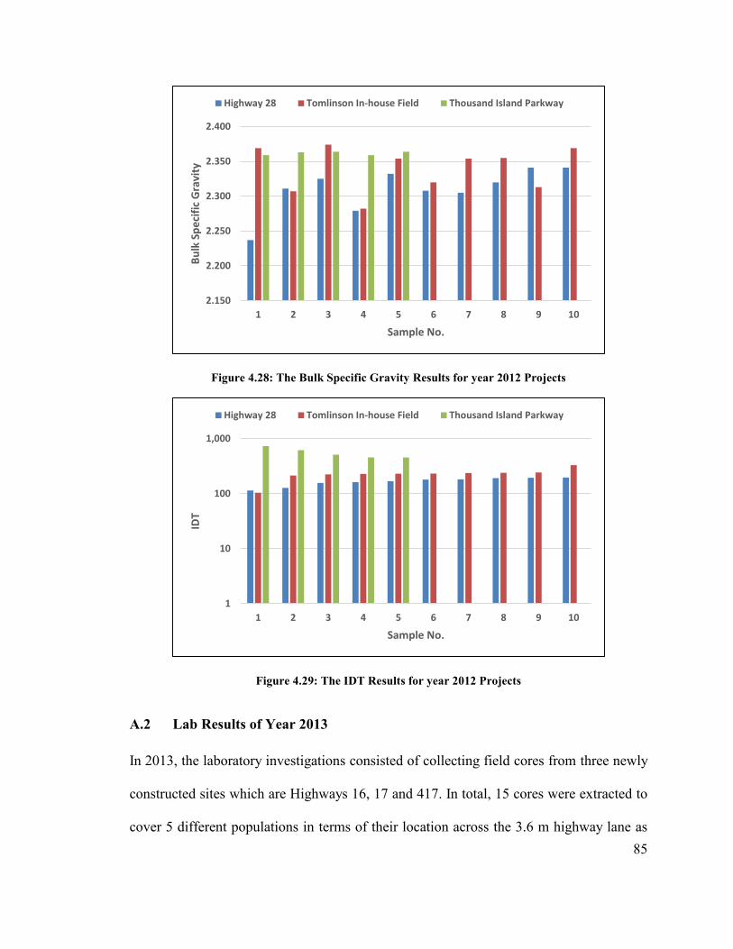
85
Figure 4.28: The Bulk Specific Gravity Results for year 2012 Projects
Figure 4.29: The IDT Results for year 2012 Projects
A.2 Lab Results of Year 2013
In 2013, the laboratory investigations consisted of collecting field cores from three newly
constructed sites which are Highways 16, 17 and 417. In total, 15 cores were extracted to
cover 5 different populations in terms of their location across the 3.6 m highway lane as
2.150
2.200
2.250
2.300
2.350
2.400
1 2 3 4 5 6 7 8 9 10
Bu
lk S
pe
cifi
c G
ravi
ty
Sample No.
Highway 28 Tomlinson In-house Field Thousand Island Parkway
1
10
100
1,000
1 2 3 4 5 6 7 8 9 10
IDT
Sample No.
Highway 28 Tomlinson In-house Field Thousand Island Parkway
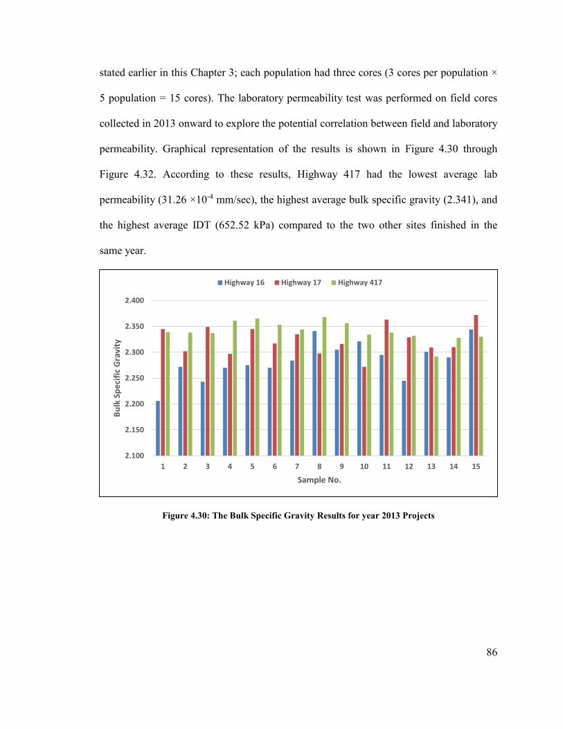
86
stated earlier in this Chapter 3; each population had three cores (3 cores per population ×
5 population = 15 cores). The laboratory permeability test was performed on field cores
collected in 2013 onward to explore the potential correlation between field and laboratory
permeability. Graphical representation of the results is shown in Figure 4.30 through
Figure 4.32. According to these results, Highway 417 had the lowest average lab
permeability (31.26 ×10⁻⁴ mm/sec), the highest average bulk specific gravity (2.341), and
the highest average IDT (652.52 kPa) compared to the two other sites finished in the
same year.
Figure 4.30: The Bulk Specific Gravity Results for year 2013 Projects
2.100
2.150
2.200
2.250
2.300
2.350
2.400
1 2 3 4 5 6 7 8 9 10 11 12 13 14 15
Bu
lk S
pe
cifi
c G
ravi
ty
Sample No.
Highway 16 Highway 17 Highway 417
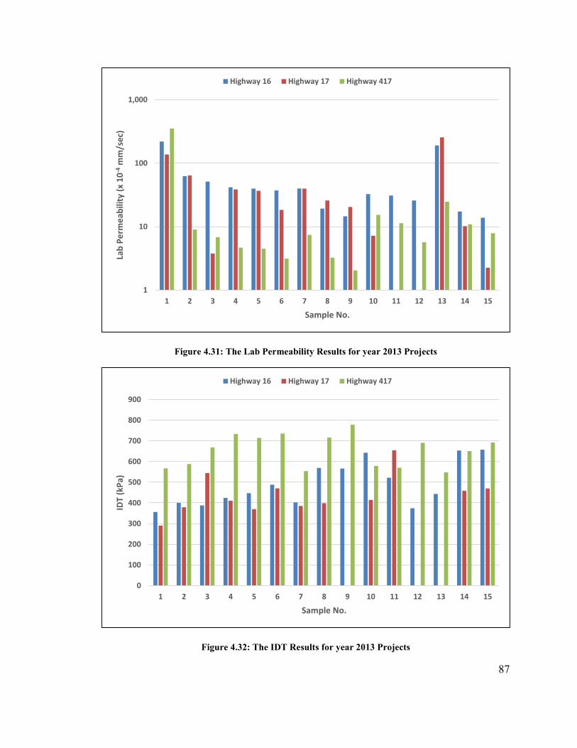
87
Figure 4.31: The Lab Permeability Results for year 2013 Projects
Figure 4.32: The IDT Results for year 2013 Projects
1
10
100
1,000
1 2 3 4 5 6 7 8 9 10 11 12 13 14 15
Lab
Pe
rme
abili
ty (
x 1
0-4
mm
/se
c)
Sample No.
Highway 16 Highway 17 Highway 417
0
100
200
300
400
500
600
700
800
900
1 2 3 4 5 6 7 8 9 10 11 12 13 14 15
IDT
(kP
a)
Sample No.
Highway 16 Highway 17 Highway 417
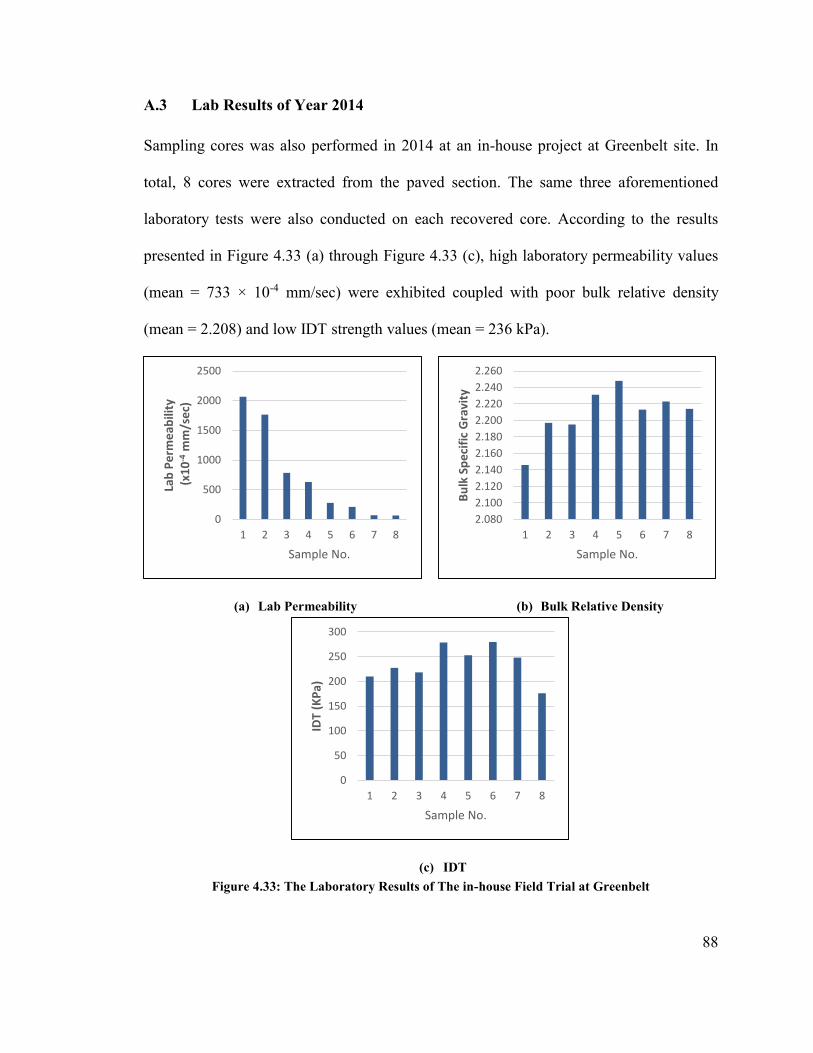
88
A.3 Lab Results of Year 2014
Sampling cores was also performed in 2014 at an in-house project at Greenbelt site. In
total, 8 cores were extracted from the paved section. The same three aforementioned
laboratory tests were also conducted on each recovered core. According to the results
presented in Figure 4.33 (a) through Figure 4.33 (c), high laboratory permeability values
(mean = 733 × 10-4 mm/sec) were exhibited coupled with poor bulk relative density
(mean = 2.208) and low IDT strength values (mean = 236 kPa).
(a) Lab Permeability (b) Bulk Relative Density
(c) IDT
Figure 4.33: The Laboratory Results of The in-house Field Trial at Greenbelt
0
500
1000
1500
2000
2500
1 2 3 4 5 6 7 8
Lab
Pe
rme
abili
ty(x
10
-4m
m/s
ec)
Sample No.
2.080
2.100
2.120
2.140
2.160
2.180
2.200
2.220
2.240
2.260
1 2 3 4 5 6 7 8
Bu
lk S
pe
cifi
c G
ravi
ty
Sample No.
0
50
100
150
200
250
300
1 2 3 4 5 6 7 8
IDT
(KP
a)
Sample No.
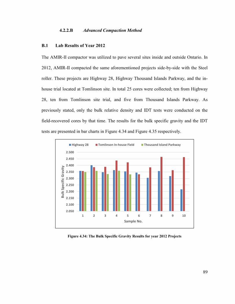
89
4.2.2.B Advanced Compaction Method
B.1 Lab Results of Year 2012
The AMIR-II compactor was utilized to pave several sites inside and outside Ontario. In
2012, AMIR-II compacted the same aforementioned projects side-by-side with the Steel
roller. These projects are Highway 28, Highway Thousand Islands Parkway, and the in-
house trial located at Tomlinson site. In total 25 cores were collected; ten from Highway
28, ten from Tomlinson site trial, and five from Thousand Islands Parkway. As
previously stated, only the bulk relative density and IDT tests were conducted on the
field-recovered cores by that time. The results for the bulk specific gravity and the IDT
tests are presented in bar charts in Figure 4.34 and Figure 4.35 respectively.
Figure 4.34: The Bulk Specific Gravity Results for year 2012 Projects
2.050
2.100
2.150
2.200
2.250
2.300
2.350
2.400
2.450
2.500
1 2 3 4 5 6 7 8 9 10
Bu
lk S
pe
cifi
c G
ravi
ty
Sample No.
Highway 28 Tomlinson In-house Field Thousand Island Parkway
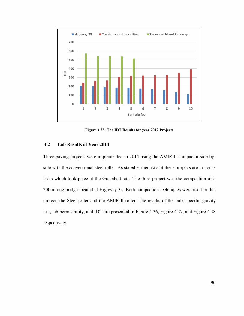
90
Figure 4.35: The IDT Results for year 2012 Projects
B.2 Lab Results of Year 2014
Three paving projects were implemented in 2014 using the AMIR-II compactor side-by-
side with the conventional steel roller. As stated earlier, two of these projects are in-house
trials which took place at the Greenbelt site. The third project was the compaction of a
200m long bridge located at Highway 34. Both compaction techniques were used in this
project, the Steel roller and the AMIR-II roller. The results of the bulk specific gravity
test, lab permeability, and IDT are presented in Figure 4.36, Figure 4.37, and Figure 4.38
respectively.
0
100
200
300
400
500
600
700
1 2 3 4 5 6 7 8 9 10
IDT
Sample No.
Highway 28 Tomlinson In-house Field Thousand Island Parkway

91
Figure 4.36: The Bulk Specific Gravity Results for year 2014 Projects
Figure 4.37: The Lab Permeability Results for year 2013 Projects
2.150
2.200
2.250
2.300
2.350
2.400
1 2 3 4 5 6 7 8 9 10 11 12 13 14
Bu
lk S
pe
cifi
c G
ravi
ty
Sample No.
Greenbelt Trial One Greenbelt Trial Two Highway 34 Bridge
1
10
100
1,000
1 2 3 4 5 6 7 8 9 10 11 12 13 14
Lab
Pe
rme
abili
ty (
x 1
0-4
mm
/se
c)
Sample No.
Greenbelt Trial One Greenbelt Trial Two Highway 34 Bridge
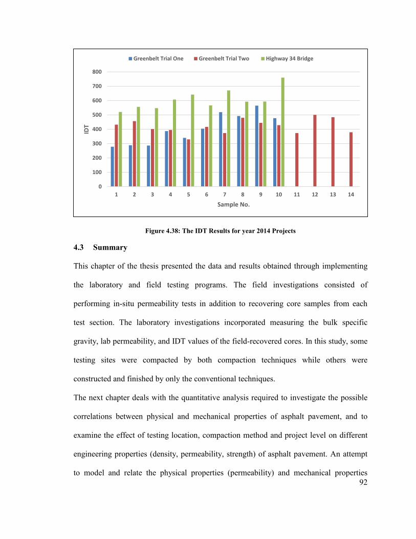
92
Figure 4.38: The IDT Results for year 2014 Projects
4.3 Summary
This chapter of the thesis presented the data and results obtained through implementing
the laboratory and field testing programs. The field investigations consisted of
performing in-situ permeability tests in addition to recovering core samples from each
test section. The laboratory investigations incorporated measuring the bulk specific
gravity, lab permeability, and IDT values of the field-recovered cores. In this study, some
testing sites were compacted by both compaction techniques while others were
constructed and finished by only the conventional techniques.
The next chapter deals with the quantitative analysis required to investigate the possible
correlations between physical and mechanical properties of asphalt pavement, and to
examine the effect of testing location, compaction method and project level on different
engineering properties (density, permeability, strength) of asphalt pavement. An attempt
to model and relate the physical properties (permeability) and mechanical properties
0
100
200
300
400
500
600
700
800
1 2 3 4 5 6 7 8 9 10 11 12 13 14
IDT
Sample No.
Greenbelt Trial One Greenbelt Trial Two Highway 34 Bridge

93
(strength) of field-recovered cores using the Gyratory compactor is carried out. Also, the
chapter studies, compares, and analyzes field and laboratory results obtained by two
different compaction methods.
94
CHAPTER 5: DATA ANALYSIS
This chapter presents the general trends and relationships of the different pavement
properties examined in this study as well as results of statistical analysis conducted on the
results obtained from both the field and laboratory investigations. The chapter consists of
five main sections. The first section illustrates and studies each asphalt pavement
property considered in this research. The second section examines the possible
correlations between the considered asphalt properties. The last three sections present the
relationship of each property to the other in two different settings; the field and
laboratory.
5.1 Physical and Mechanical Properties of Asphalt Pavement
This section is devoted to present the analysis of different physical and mechanical
properties as well as comparing the performance of the two compaction techniques in
terms of these properties. Particularly, the obtained field and laboratory results at the five
testing locations introduced earlier in Chapter 3 were used to construct the comparison. In
this research, the impact of three different independent factors including the testing
location, compaction method, and project level on each pavement property (response
variable) was examined. Subsequently, a three-way ANOVA test at 5% level of
significance was used in Section 5.1.1 through Section 5.1.4 to examine the possible
three-way and two-way interaction effects between the three considered factors. For
further investigation purposes, the three-way ANOVA was followed in some cases by
one-way ANOVA test at 5% level of significance to determine if the compaction method
has a statistically significant effect on the quality of the each pavement property. Before
conducting any of the statistical tests in this chapter, the test of homogeneity of variances
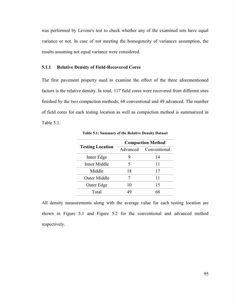
95
was performed by Levene's test to check whether any of the examined sets have equal
variance or not. In case of not meeting the homogeneity of variances assumption, the
results assuming not equal variance were considered.
5.1.1 Relative Density of Field-Recovered Cores
The first pavement property used to examine the effect of the three aforementioned
factors is the relative density. In total, 117 field cores were recovered from different sites
finished by the two compaction methods; 68 conventional and 49 advanced. The number
of field cores for each testing location as well as compaction method is summarized in
Table 5.1.
Table 5.1: Summary of the Relative Density Dataset
Testing Location Compaction Method
Advanced Conventional
Inner Edge 9 14
Inner Middle 5 11
Middle 18 17
Outer Middle 7 11
Outer Edge 10 15
Total 49 68
All density measurements along with the average value for each testing location are
shown in Figure 5.1 and Figure 5.2 for the conventional and advanced method
respectively.
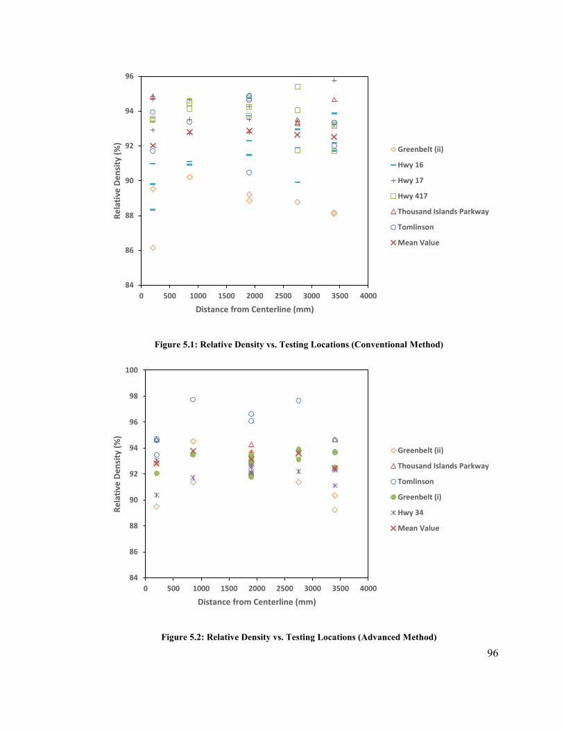
96
Figure 5.1: Relative Density vs. Testing Locations (Conventional Method)
Figure 5.2: Relative Density vs. Testing Locations (Advanced Method)
84
86
88
90
92
94
96
0 500 1000 1500 2000 2500 3000 3500 4000
Re
lati
ve D
en
sity
(%
)
Distance from Centerline (mm)
Greenbelt (ii)
Hwy 16
Hwy 17
Hwy 417
Thousand Islands Parkway
Tomlinson
Mean Value
84
86
88
90
92
94
96
98
100
0 500 1000 1500 2000 2500 3000 3500 4000
Re
lati
ve D
en
sity
(%
)
Distance from Centerline (mm)
Greenbelt (ii)
Thousand Islands Parkway
Tomlinson
Greenbelt (i)
Hwy 34
Mean Value
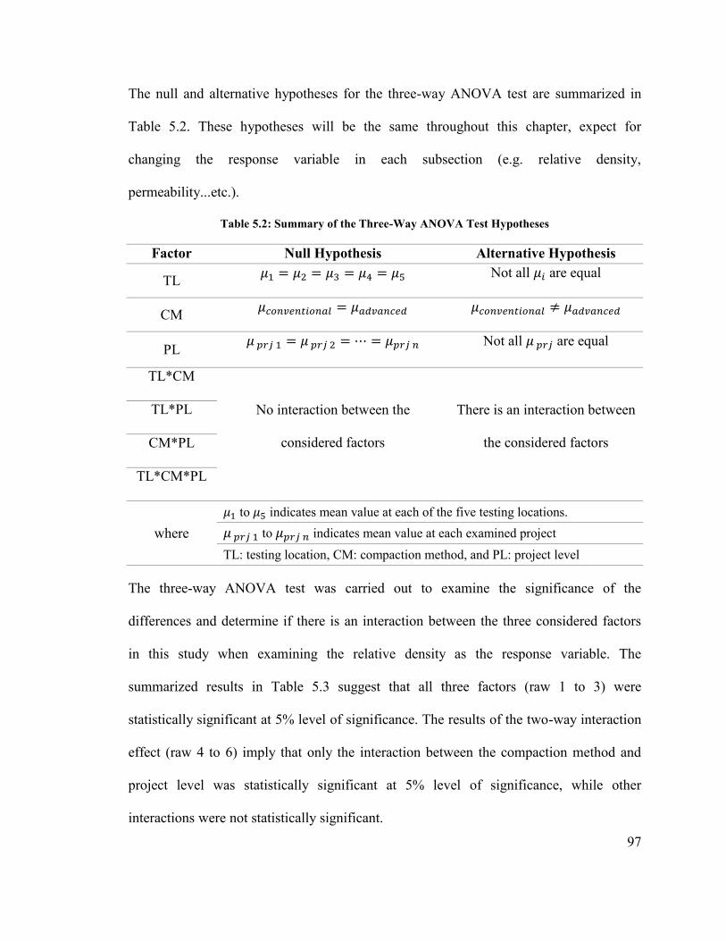
97
The null and alternative hypotheses for the three-way ANOVA test are summarized in
Table 5.2. These hypotheses will be the same throughout this chapter, expect for
changing the response variable in each subsection (e.g. relative density,
permeability...etc.).
Table 5.2: Summary of the Three-Way ANOVA Test Hypotheses
Factor Null Hypothesis Alternative Hypothesis
TL 𝜇1 = 𝜇2 = 𝜇3 = 𝜇4 = 𝜇5 Not all 𝜇𝑖 are equal
CM 𝜇𝑐𝑜𝑛𝑣𝑒𝑛𝑡𝑖𝑜𝑛𝑎𝑙 = 𝜇𝑎𝑑𝑣𝑎𝑛𝑐𝑒𝑑 𝜇𝑐𝑜𝑛𝑣𝑒𝑛𝑡𝑖𝑜𝑛𝑎𝑙 ≠ 𝜇𝑎𝑑𝑣𝑎𝑛𝑐𝑒𝑑
PL 𝜇 𝑝𝑟𝑗 1 = 𝜇 𝑝𝑟𝑗 2 = ⋯ = 𝜇𝑝𝑟𝑗 𝑛 Not all 𝜇 𝑝𝑟𝑗 are equal
TL*CM
No interaction between the
considered factors
There is an interaction between
the considered factors
TL*PL
CM*PL
TL*CM*PL
where
𝜇1 to 𝜇5 indicates mean value at each of the five testing locations.
𝜇 𝑝𝑟𝑗 1 to 𝜇𝑝𝑟𝑗 𝑛 indicates mean value at each examined project
TL: testing location, CM: compaction method, and PL: project level
The three-way ANOVA test was carried out to examine the significance of the
differences and determine if there is an interaction between the three considered factors
in this study when examining the relative density as the response variable. The
summarized results in Table 5.3 suggest that all three factors (raw 1 to 3) were
statistically significant at 5% level of significance. The results of the two-way interaction
effect (raw 4 to 6) imply that only the interaction between the compaction method and
project level was statistically significant at 5% level of significance, while other
interactions were not statistically significant.
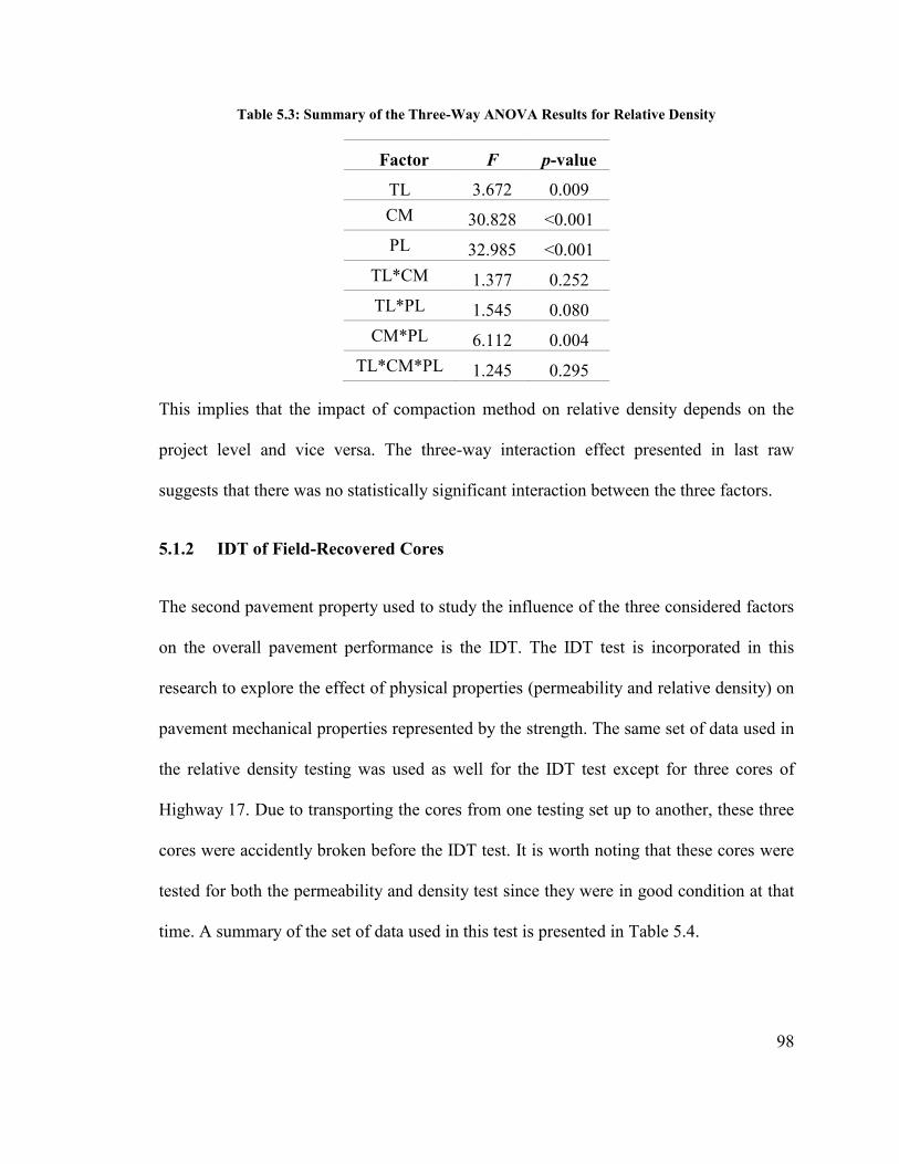
98
Table 5.3: Summary of the Three-Way ANOVA Results for Relative Density
Factor F p-value
TL 3.672 0.009
CM 30.828 <0.001
PL 32.985 <0.001
TL*CM 1.377 0.252
TL*PL 1.545 0.080
CM*PL 6.112 0.004
TL*CM*PL 1.245 0.295
This implies that the impact of compaction method on relative density depends on the
project level and vice versa. The three-way interaction effect presented in last raw
suggests that there was no statistically significant interaction between the three factors.
5.1.2 IDT of Field-Recovered Cores
The second pavement property used to study the influence of the three considered factors
on the overall pavement performance is the IDT. The IDT test is incorporated in this
research to explore the effect of physical properties (permeability and relative density) on
pavement mechanical properties represented by the strength. The same set of data used in
the relative density testing was used as well for the IDT test except for three cores of
Highway 17. Due to transporting the cores from one testing set up to another, these three
cores were accidently broken before the IDT test. It is worth noting that these cores were
tested for both the permeability and density test since they were in good condition at that
time. A summary of the set of data used in this test is presented in Table 5.4.
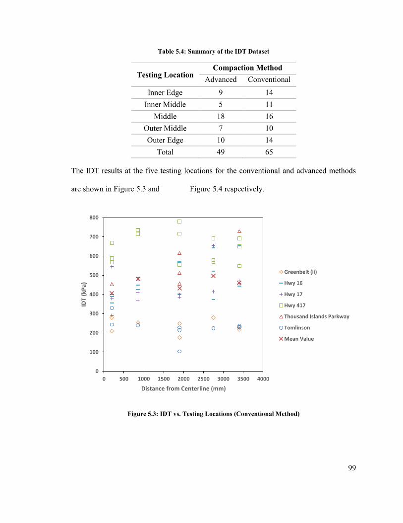
99
Table 5.4: Summary of the IDT Dataset
Testing Location Compaction Method
Advanced Conventional
Inner Edge 9 14
Inner Middle 5 11
Middle 18 16
Outer Middle 7 10
Outer Edge 10 14
Total 49 65
The IDT results at the five testing locations for the conventional and advanced methods
are shown in Figure 5.3 and Figure 5.4 respectively.
Figure 5.3: IDT vs. Testing Locations (Conventional Method)
0
100
200
300
400
500
600
700
800
0 500 1000 1500 2000 2500 3000 3500 4000
IDT
(kP
a)
Distance from Centerline (mm)
Greenbelt (ii)
Hwy 16
Hwy 17
Hwy 417
Thousand Islands Parkway
Tomlinson
Mean Value
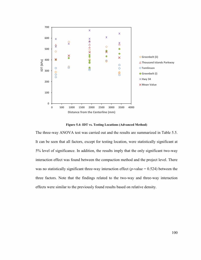
100
Figure 5.4: IDT vs. Testing Locations (Advanced Method)
The three-way ANOVA test was carried out and the results are summarized in Table 5.5.
It can be seen that all factors, except for testing location, were statistically significant at
5% level of significance. In addition, the results imply that the only significant two-way
interaction effect was found between the compaction method and the project level. There
was no statistically significant three-way interaction effect (p-value = 0.524) between the
three factors. Note that the findings related to the two-way and three-way interaction
effects were similar to the previously found results based on relative density.
0
100
200
300
400
500
600
700
0 500 1000 1500 2000 2500 3000 3500 4000
IDT
(kP
a)
Distance from the Centerline (mm)
Greenbelt (ii)
Thousand Islands Parkway
Tomlinson
Greenbelt (i)
Hwy 34
Mean Value
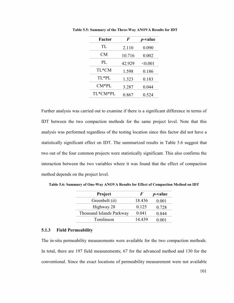
101
Table 5.5: Summary of the Three-Way ANOVA Results for IDT
Factor F p-value
TL 2.110 0.090
CM 10.716 0.002
PL 42.929 <0.001
TL*CM 1.598 0.186
TL*PL 1.323 0.183
CM*PL 3.287 0.044
TL*CM*PL 0.867 0.524
Further analysis was carried out to examine if there is a significant difference in terms of
IDT between the two compaction methods for the same project level. Note that this
analysis was performed regardless of the testing location since this factor did not have a
statistically significant effect on IDT. The summarized results in Table 5.6 suggest that
two out of the four common projects were statistically significant. This also confirms the
interaction between the two variables where it was found that the effect of compaction
method depends on the project level.
Table 5.6: Summary of One-Way ANOVA Results for Effect of Compaction Method on IDT
Project F p-value
Greenbelt (ii) 18.436 0.001
Highway 28 0.125 0.728
Thousand Islands Parkway 0.041 0.844
Tomlinson 14.439 0.001
5.1.3 Field Permeability
The in-situ permeability measurements were available for the two compaction methods.
In total, there are 197 field measurements; 67 for the advanced method and 130 for the
conventional. Since the exact locations of permeability measurement were not available
102
for one common site (Highway 28) for the two compaction method, 20 field
measurements were excluded in this analysis; 10 for each compaction method. This
results in having 57 field permeability measurements for the advanced method and 120
for the conventional. Table 5.7 summarizes the numbers of field permeability
measurements for each compaction technique and their corresponding testing locations.
Note that no field permeability measurements were taken at the inner middle or outer
inner locations for the advanced method.
Table 5.7: Summary of the Field Permeability Dataset
Testing Location Compaction Method
Advanced Conventional
Inner Edge 14 33
Inner Middle - 13
Middle 28 34
Outer Middle - 13
Outer Edge 15 27
Total 57 120
Figure 5.5 and Figure 5.6 show all permeability measurements at the five test locations
for the conventional and advanced method respectively. According to the presented
results, on average the inner edge location of the conventional method experiences
relatively higher permeability compared to the other testing locations of the same
compaction method. In general, the field permeability trend of the conventional method
showed that the middle locations, except for the outer middle location, have less
permeability compared to the three other locations. Note that the outer middle is higher
than the outer edge due to the influence of one single measurement. For the advanced
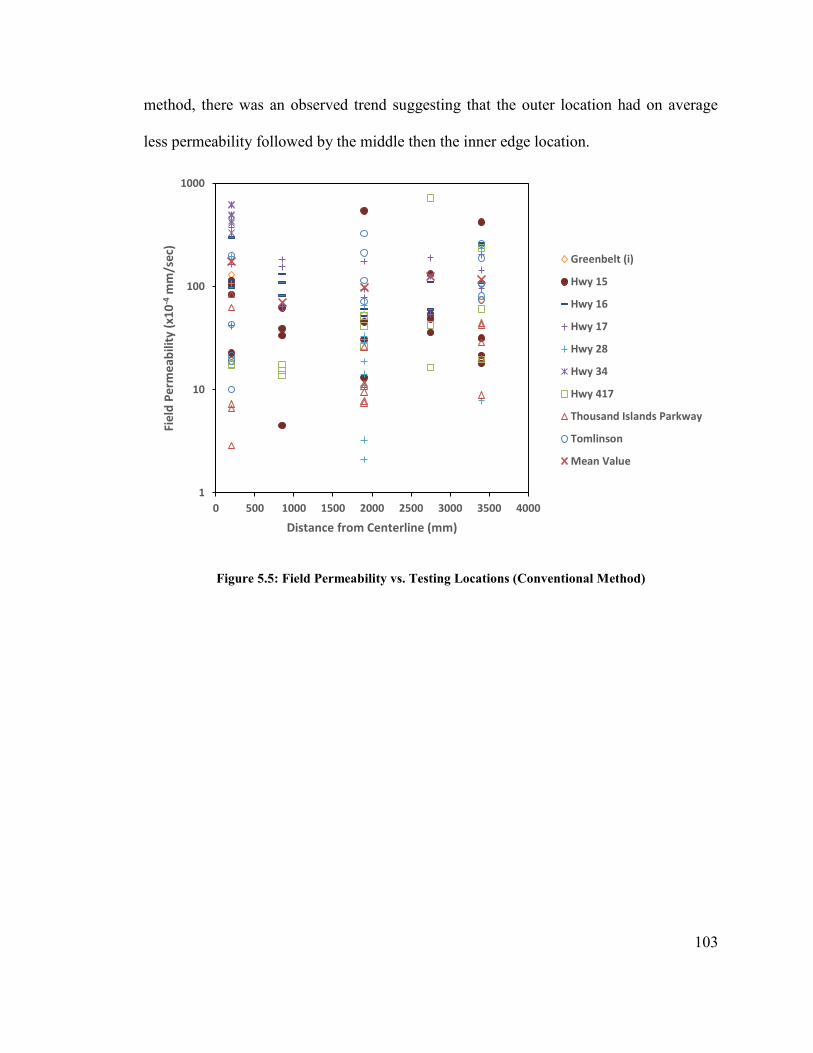
103
method, there was an observed trend suggesting that the outer location had on average
less permeability followed by the middle then the inner edge location.
Figure 5.5: Field Permeability vs. Testing Locations (Conventional Method)
1
10
100
1000
0 500 1000 1500 2000 2500 3000 3500 4000
Fie
ld P
erm
eab
ility
(x1
0-4
mm
/se
c)
Distance from Centerline (mm)
Greenbelt (i)
Hwy 15
Hwy 16
Hwy 17
Hwy 28
Hwy 34
Hwy 417
Thousand Islands Parkway
Tomlinson
Mean Value
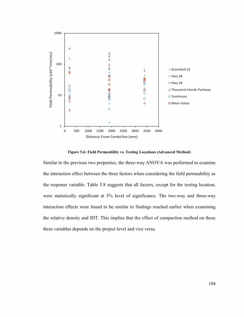
104
Figure 5.6: Field Permeability vs. Testing Locations (Advanced Method)
Similar to the previous two properties, the three-way ANOVA was performed to examine
the interaction effect between the three factors when considering the field permeability as
the response variable. Table 5.8 suggests that all factors, except for the testing location,
were statistically significant at 5% level of significance. The two-way and three-way
interaction effects were found to be similar to findings reached earlier when examining
the relative density and IDT. This implies that the effect of compaction method on these
three variables depends on the project level and vice versa.
1
10
100
1000
0 500 1000 1500 2000 2500 3000 3500 4000
Fie
ld P
erm
eab
ility
(x1
0-4
mm
/se
c)
Distance From Centerline (mm)
Greenbelt (i)
Hwy 28
Hwy 34
Thousand Islands Parkway
Tomlinson
Mean Value
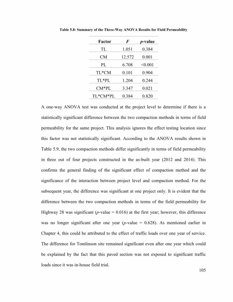
105
Table 5.8: Summary of the Three-Way ANOVA Results for Field Permeability
Factor F p-value
TL 1.051 0.384
CM 12.572 0.001
PL 6.708 <0.001
TL*CM 0.101 0.904
TL*PL 1.204 0.244
CM*PL 3.347 0.021
TL*CM*PL 0.384 0.820
A one-way ANOVA test was conducted at the project level to determine if there is a
statistically significant difference between the two compaction methods in terms of field
permeability for the same project. This analysis ignores the effect testing location since
this factor was not statistically significant. According to the ANOVA results shown in
Table 5.9, the two compaction methods differ significantly in terms of field permeability
in three out of four projects constructed in the as-built year (2012 and 2014). This
confirms the general finding of the significant effect of compaction method and the
significance of the interaction between project level and compaction method. For the
subsequent year, the difference was significant at one project only. It is evident that the
difference between the two compaction methods in terms of the field permeability for
Highway 28 was significant (p-value = 0.016) at the first year; however, this difference
was no longer significant after one year (p-value = 0.628). As mentioned earlier in
Chapter 4, this could be attributed to the effect of traffic loads over one year of service.
The difference for Tomlinson site remained significant even after one year which could
be explained by the fact that this paved section was not exposed to significant traffic
loads since it was in-house field trial.
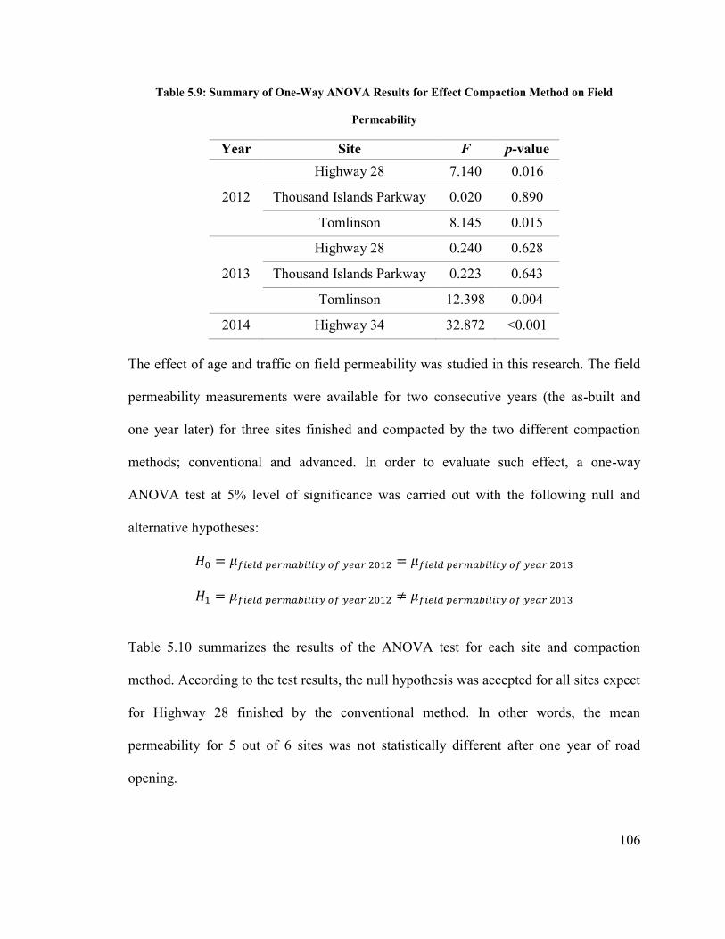
106
Table 5.9: Summary of One-Way ANOVA Results for Effect Compaction Method on Field
Permeability
Year Site F p-value
2012
Highway 28 7.140 0.016
Thousand Islands Parkway 0.020 0.890
Tomlinson 8.145 0.015
2013
Highway 28 0.240 0.628
Thousand Islands Parkway 0.223 0.643
Tomlinson 12.398 0.004
2014 Highway 34 32.872 <0.001
The effect of age and traffic on field permeability was studied in this research. The field
permeability measurements were available for two consecutive years (the as-built and
one year later) for three sites finished and compacted by the two different compaction
methods; conventional and advanced. In order to evaluate such effect, a one-way
ANOVA test at 5% level of significance was carried out with the following null and
alternative hypotheses:
𝐻0 = 𝜇𝑓𝑖𝑒𝑙𝑑 𝑝𝑒𝑟𝑚𝑎𝑏𝑖𝑙𝑖𝑡𝑦 𝑜𝑓 𝑦𝑒𝑎𝑟 2012 = 𝜇𝑓𝑖𝑒𝑙𝑑 𝑝𝑒𝑟𝑚𝑎𝑏𝑖𝑙𝑖𝑡𝑦 𝑜𝑓 𝑦𝑒𝑎𝑟 2013
𝐻1 = 𝜇𝑓𝑖𝑒𝑙𝑑 𝑝𝑒𝑟𝑚𝑎𝑏𝑖𝑙𝑖𝑡𝑦 𝑜𝑓 𝑦𝑒𝑎𝑟 2012 ≠ 𝜇𝑓𝑖𝑒𝑙𝑑 𝑝𝑒𝑟𝑚𝑎𝑏𝑖𝑙𝑖𝑡𝑦 𝑜𝑓 𝑦𝑒𝑎𝑟 2013
Table 5.10 summarizes the results of the ANOVA test for each site and compaction
method. According to the test results, the null hypothesis was accepted for all sites expect
for Highway 28 finished by the conventional method. In other words, the mean
permeability for 5 out of 6 sites was not statistically different after one year of road
opening.

107
Table 5.10: Summary of the t-test Results for Effect of Age and Traffic on Field Permeability
Site Name Conventional Advanced
F p-value F p-value
Highway 28 8.838 0.007 0.277 0.603
Thousand Islands Parkway 2.988 0.106 3.822 0.069
Tomlinson 0.667 0.429 0.103 0.753
5.1.4 Laboratory Permeability of Field-Recovered Cores
The results obtained by performing the laboratory tests on a total of 86 field-recovered
cores (34 advanced and 52 conventional) were used for the purpose of comparison
between the two compaction techniques. It is worth noting that out of the 117 cores tested
for relative density, 31 cores were not tested for lab permeability test since the testing
device was not available in Carleton lab by that time. Table 5.11 summarizes the numbers
of field cores per testing location for the two compaction methods.
Table 5.11: Summary of the Lab Permeability Dataset
Testing Location Compaction Method
Advanced Conventional
Inner Edge 5 11
Inner Middle 4 10
Middle 13 11
Outer Middle 6 9
Outer Edge 6 11
Total 34 52
All lab permeability measurements for the conventional and advanced methods at the five
testing locations are presented graphically in Figure 5.7 and Figure 5.8 respectively
According to the presented bar chart, there is an obvious decrease in mean permeability
values in the three middle locations compared to the lane edges. On the other hand, outer
and inner edges experienced relatively high permeability compared to the middle

108
locations. This observations holds true for the two compaction methods. In addition, the
presented results suggest that the field cores recovered from road sections finished by the
advanced method are, on average, less permeable in all considered locations compared to
the conventional method.
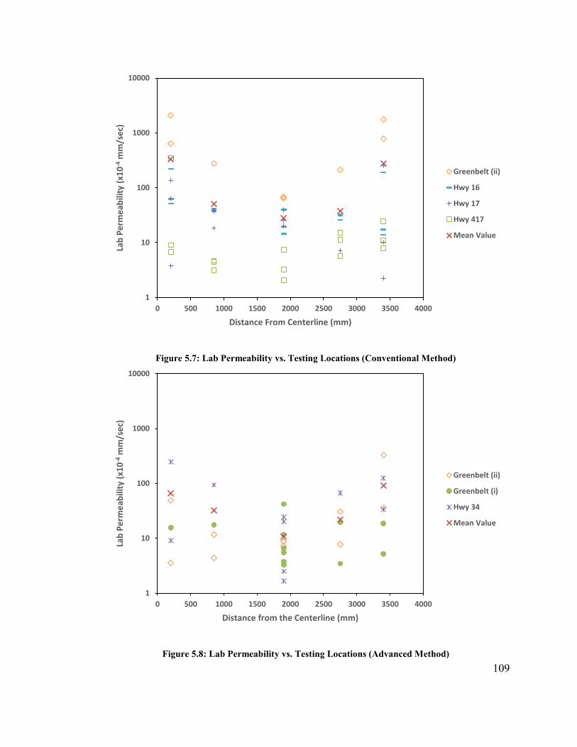
109
Figure 5.7: Lab Permeability vs. Testing Locations (Conventional Method)
Figure 5.8: Lab Permeability vs. Testing Locations (Advanced Method)
1
10
100
1000
10000
0 500 1000 1500 2000 2500 3000 3500 4000
Lab
Pe
rme
abili
ty (
x10
-4m
m/s
ec)
Distance From Centerline (mm)
Greenbelt (ii)
Hwy 16
Hwy 17
Hwy 417
Mean Value
1
10
100
1000
10000
0 500 1000 1500 2000 2500 3000 3500 4000
Lab
Pe
rme
abili
ty (
x10
-4m
m/s
ec)
Distance from the Centerline (mm)
Greenbelt (ii)
Greenbelt (i)
Hwy 34
Mean Value
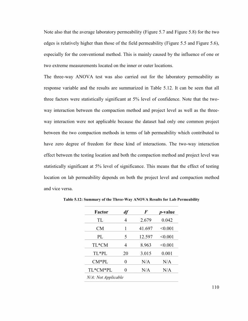
110
Note also that the average laboratory permeability (Figure 5.7 and Figure 5.8) for the two
edges is relatively higher than those of the field permeability (Figure 5.5 and Figure 5.6),
especially for the conventional method. This is mainly caused by the influence of one or
two extreme measurements located on the inner or outer locations.
The three-way ANOVA test was also carried out for the laboratory permeability as
response variable and the results are summarized in Table 5.12. It can be seen that all
three factors were statistically significant at 5% level of confidence. Note that the two-
way interaction between the compaction method and project level as well as the three-
way interaction were not applicable because the dataset had only one common project
between the two compaction methods in terms of lab permeability which contributed to
have zero degree of freedom for these kind of interactions. The two-way interaction
effect between the testing location and both the compaction method and project level was
statistically significant at 5% level of significance. This means that the effect of testing
location on lab permeability depends on both the project level and compaction method
and vice versa.
Table 5.12: Summary of the Three-Way ANOVA Results for Lab Permeability
Factor df F p-value
TL 4 2.679 0.042
CM 1 41.697 <0.001
PL 5 12.597 <0.001
TL*CM 4 8.963 <0.001
TL*PL 20 3.015 0.001
CM*PL 0 N/A N/A
TL*CM*PL 0 N/A N/A
N/A: Not Applicable
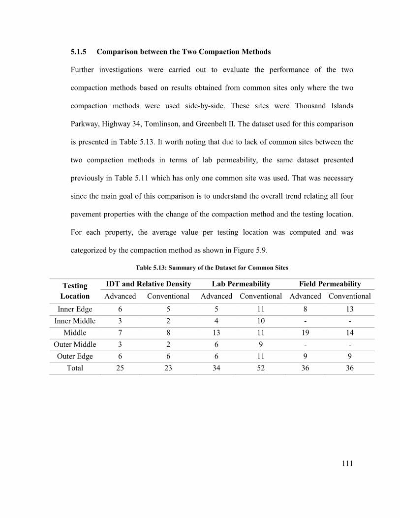
111
5.1.5 Comparison between the Two Compaction Methods
Further investigations were carried out to evaluate the performance of the two
compaction methods based on results obtained from common sites only where the two
compaction methods were used side-by-side. These sites were Thousand Islands
Parkway, Highway 34, Tomlinson, and Greenbelt II. The dataset used for this comparison
is presented in Table 5.13. It worth noting that due to lack of common sites between the
two compaction methods in terms of lab permeability, the same dataset presented
previously in Table 5.11 which has only one common site was used. That was necessary
since the main goal of this comparison is to understand the overall trend relating all four
pavement properties with the change of the compaction method and the testing location.
For each property, the average value per testing location was computed and was
categorized by the compaction method as shown in Figure 5.9.
Table 5.13: Summary of the Dataset for Common Sites
Testing
Location
IDT and Relative Density Lab Permeability Field Permeability
Advanced Conventional Advanced Conventional Advanced Conventional
Inner Edge 6 5 5 11 8 13
Inner Middle 3 2 4 10 - -
Middle 7 8 13 11 19 14
Outer Middle 3 2 6 9 - -
Outer Edge 6 6 6 11 9 9
Total 25 23 34 52 36 36
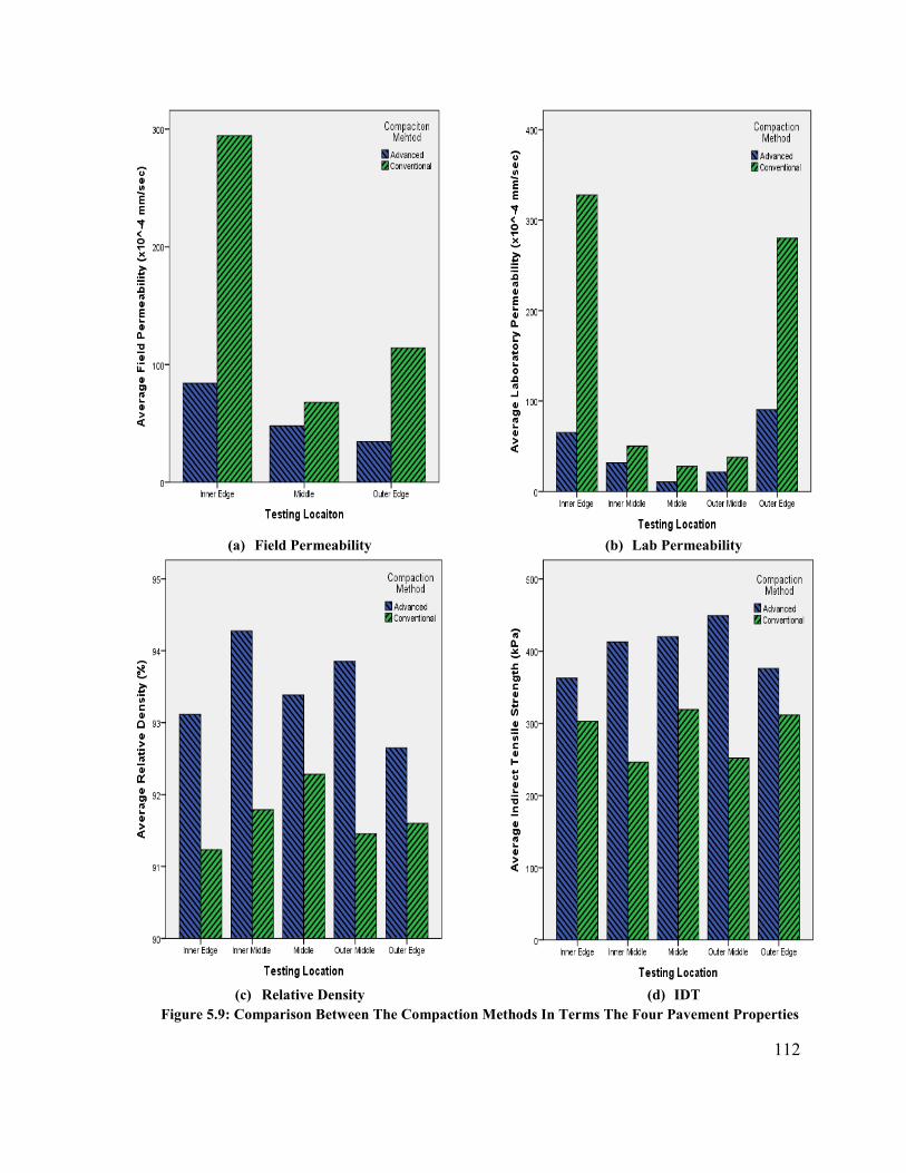
112
(a) Field Permeability (b) Lab Permeability
(c) Relative Density (d) IDT
Figure 5.9: Comparison Between The Compaction Methods In Terms The Four Pavement Properties
113
For the field permeability Figure 5.9 (a), the observed trend for the conventional method
suggests that the two edges had higher average permeability than the middle location.
The advanced method showed that there was a gradual reduction in average permeability
as moving from the inner edge to the outer. In all cases, it is quite evident that the field
permeability values for the conventional method were higher than those of the advanced
method. Figure 5.9 (b) suggests that there was an obvious decrease in average lab
permeability values where the outer and inner edges experienced relatively high
permeability compared to the middle locations. This observation holds true for the two
compaction methods. In addition, the presented results imply that the field-recovered
cores obtained from road sections finished by the advanced method are, on average, less
permeable in all considered locations compared to the conventional method. The bar
chart presented in Figure 5.9 (c) shows that the observed trend of the conventional
method indicates that the relative density was higher at the middle and it decreases
gradually at the two lane edges. For the advanced method, it was found that the inner
middle and outer middle have on average the highest relative density followed by the
middle location and the two edge locations. According to the IDT results shown in
Figure 5.9 (d), the conventional method showed less strength in the inner and outer
middle locations while the other three locations were almost equal. The advanced
technique exhibited a gradual trend where the IDT values are higher in the three middle
locations compared to the two edges.
114
A one-way ANOVA test was also conducted to investigate if there is a significant
difference between the mean values for each property of the two compaction methods.
The null and alternative hypotheses for each property are shown in Table 5.14.
Table 5.14: Summary of the Null and Alternative Hypotheses for Common Sites
Property Test Hypotheses
Null Alternative
Field Permeability
𝜇𝑐𝑜𝑛𝑣𝑒𝑛𝑡𝑖𝑜𝑛𝑎𝑙 = 𝜇𝑎𝑑𝑣𝑎𝑛𝑐𝑒𝑑 𝜇𝑐𝑜𝑛𝑣𝑒𝑛𝑡𝑖𝑜𝑛𝑎𝑙 ≠ 𝜇𝑎𝑑𝑣𝑎𝑛𝑐𝑒𝑑 Lab Permeability
Relative Density
IDT
According to the ANOVA results summarized in Table 5.15, it can be seen that all p-
values were less than 5% and the null hypothesis was rejected. This indicates that there
was a significant difference between the two compaction methods in terms of the four
considered properties in this study when examining the common sites between them only.
Table 5.15: Summary of the One-way ANOVA Results for the common sites
Response Factor F p-value
Field Permeability 17.752 <0.001
Lab Permeability 4.253 0.044
Relative Density 8.675 0.004
IDT 4.311 0.042
5.2 Correlations between the Physical and Mechanical Properties
The correlations between the four asphalt pavement properties considered in this research
were investigated using Pearson product-moment correlation or Pearson’s correlation,
denoted as “r”. In general, the Pearson's correlation coefficient ranges between -1 and 1
and it represents the association between two variables. The Pearson’s correlation
115
coefficient can also be tested for significance with the null and alternative hypothesis
formulated as follow:
𝐻0: 𝑟 = 0 ; the correlation between the two variables is not statistically significant
𝐻1: 𝑟 ≠ 0 ; the correlation between the two variables is statistically significant
The correlations between the different properties were examined for each compaction
method separately. First, the results produced by the Gyratory compactor was analyzed,
followed by the two field compaction methods, the conventional and advanced
compactor.
5.2.1 SGC Samples
The correlation matrix for the SGC specimens is presented in Table 5.16. The lab
permeability had strong negative correlation with both the IDT and relative density.
These two correlations were statistically significant at 5% level of significance. There
was also very strong positive correlation (r = 0.913) between the relative density and
IDT; this relationship was also statistically significant.
Table 5.16: Summary of the Correlation Coefficients and p-values for SGC Samples
Lab Permeability IDT Relative Density
Lab Permeability 1 -0.651(<0.001) -0.743(<0.001)
IDT -0.651(<0.001) 1 0.913(<0.001)
Relative Density -0.743(<0.001) 0.913(<0.001) 1
5.2.2 Field-Recovered Cores
Table 5.17 shows the correlation matrix for the field-recovered cores of the conventional
method. It can be seen that the field permeability had moderate positive correlation with
the lab permeability. In addition, the field permeability correlated negatively with both
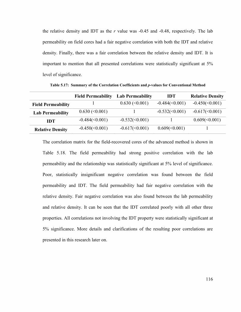
116
the relative density and IDT as the r value was -0.45 and -0.48, respectively. The lab
permeability on field cores had a fair negative correlation with both the IDT and relative
density. Finally, there was a fair correlation between the relative density and IDT. It is
important to mention that all presented correlations were statistically significant at 5%
level of significance.
Table 5.17: Summary of the Correlation Coefficients and p-values for Conventional Method
Field Permeability Lab Permeability IDT Relative Density
Field Permeability 1 0.630 (<0.001) -0.484(<0.001) -0.450(<0.001)
Lab Permeability 0.630 (<0.001) 1 -0.532(<0.001) -0.617(<0.001)
IDT -0.484(<0.001) -0.532(<0.001) 1 0.609(<0.001)
Relative Density -0.450(<0.001) -0.617(<0.001) 0.609(<0.001) 1
The correlation matrix for the field-recovered cores of the advanced method is shown in
Table 5.18. The field permeability had strong positive correlation with the lab
permeability and the relationship was statistically significant at 5% level of significance.
Poor, statistically insignificant negative correlation was found between the field
permeability and IDT. The field permeability had fair negative correlation with the
relative density. Fair negative correlation was also found between the lab permeability
and relative density. It can be seen that the IDT correlated poorly with all other three
properties. All correlations not involving the IDT property were statistically significant at
5% significance. More details and clarifications of the resulting poor correlations are
presented in this research later on.
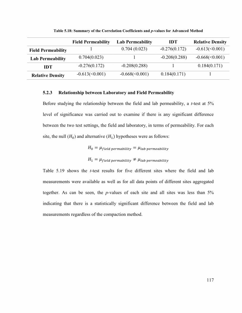
117
Table 5.18: Summary of the Correlation Coefficients and p-values for Advanced Method
Field Permeability Lab Permeability IDT Relative Density
Field Permeability 1 0.704 (0.023) -0.276(0.172) -0.613(<0.001)
Lab Permeability 0.704(0.023) 1 -0.208(0.288) -0.668(<0.001)
IDT -0.276(0.172) -0.208(0.288) 1 0.184(0.171)
Relative Density -0.613(<0.001) -0.668(<0.001) 0.184(0.171) 1
5.2.3 Relationship between Laboratory and Field Permeability
Before studying the relationship between the field and lab permeability, a t-test at 5%
level of significance was carried out to examine if there is any significant difference
between the two test settings, the field and laboratory, in terms of permeability. For each
site, the null (𝐻0) and alternative (𝐻1) hypotheses were as follows:
𝐻0 = 𝜇𝑓𝑖𝑒𝑙𝑑 𝑝𝑒𝑟𝑚𝑎𝑏𝑖𝑙𝑖𝑡𝑦 = 𝜇𝑙𝑎𝑏 𝑝𝑒𝑟𝑚𝑒𝑎𝑏𝑖𝑙𝑖𝑡𝑦
𝐻1 = 𝜇𝑓𝑖𝑒𝑙𝑑 𝑝𝑒𝑟𝑚𝑎𝑏𝑖𝑙𝑖𝑡𝑦 ≠ 𝜇𝑙𝑎𝑏 𝑝𝑒𝑟𝑚𝑒𝑎𝑏𝑖𝑙𝑖𝑡𝑦
Table 5.19 shows the t-test results for five different sites where the field and lab
measurements were available as well as for all data points of different sites aggregated
together. As can be seen, the p-values of each site and all sites was less than 5%
indicating that there is a statistically significant difference between the field and lab
measurements regardless of the compaction method.
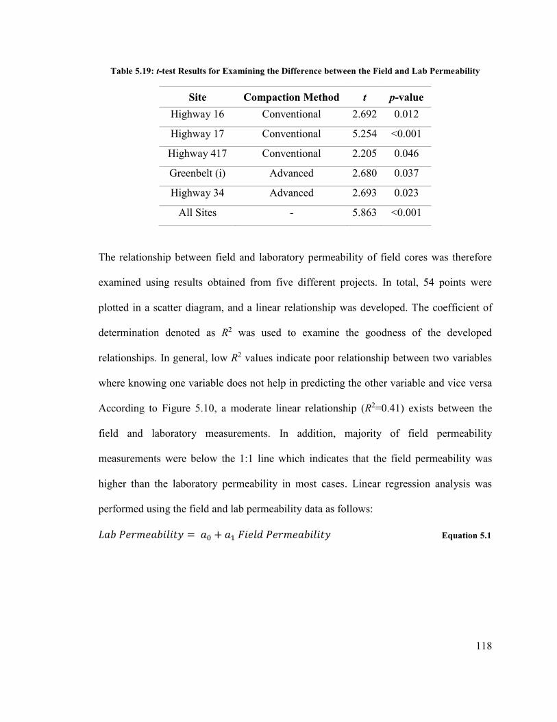
118
Table 5.19: t-test Results for Examining the Difference between the Field and Lab Permeability
Site Compaction Method t p-value
Highway 16 Conventional 2.692 0.012
Highway 17 Conventional 5.254 <0.001
Highway 417 Conventional 2.205 0.046
Greenbelt (i) Advanced 2.680 0.037
Highway 34 Advanced 2.693 0.023
All Sites - 5.863 <0.001
The relationship between field and laboratory permeability of field cores was therefore
examined using results obtained from five different projects. In total, 54 points were
plotted in a scatter diagram, and a linear relationship was developed. The coefficient of
determination denoted as R2 was used to examine the goodness of the developed
relationships. In general, low R2 values indicate poor relationship between two variables
where knowing one variable does not help in predicting the other variable and vice versa
According to Figure 5.10, a moderate linear relationship (R2=0.41) exists between the
field and laboratory measurements. In addition, majority of field permeability
measurements were below the 1:1 line which indicates that the field permeability was
higher than the laboratory permeability in most cases. Linear regression analysis was
performed using the field and lab permeability data as follows:
𝐿𝑎𝑏 𝑃𝑒𝑟𝑚𝑒𝑎𝑏𝑖𝑙𝑖𝑡𝑦 = 𝑎0 + 𝑎1 𝐹𝑖𝑒𝑙𝑑 𝑃𝑒𝑟𝑚𝑒𝑎𝑏𝑖𝑙𝑖𝑡𝑦 Equation 5.1
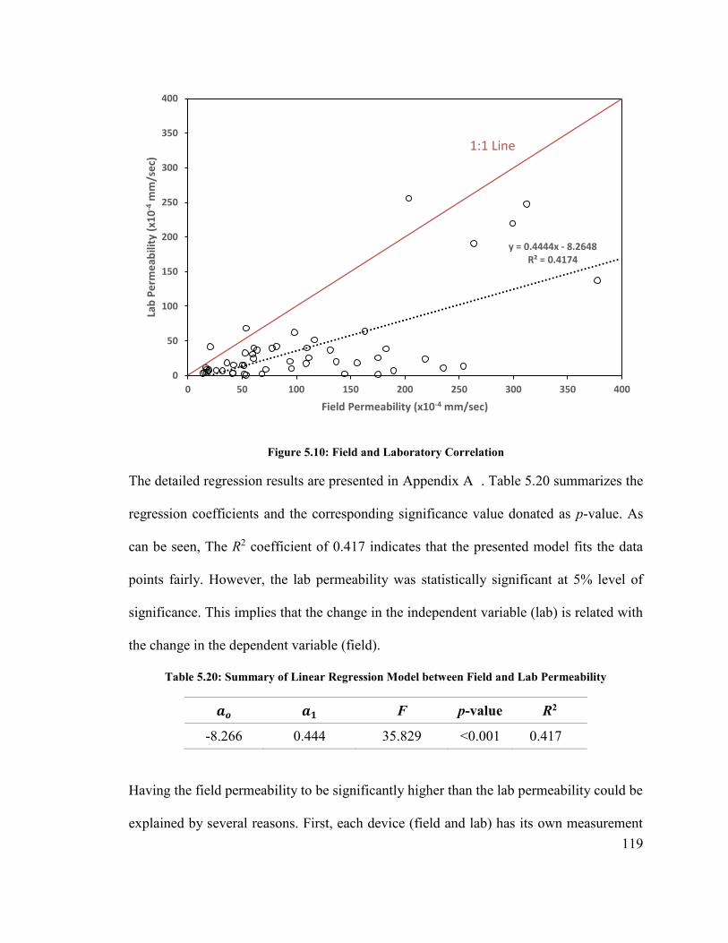
119
Figure 5.10: Field and Laboratory Correlation
The detailed regression results are presented in Appendix A . Table 5.20 summarizes the
regression coefficients and the corresponding significance value donated as p-value. As
can be seen, The R2 coefficient of 0.417 indicates that the presented model fits the data
points fairly. However, the lab permeability was statistically significant at 5% level of
significance. This implies that the change in the independent variable (lab) is related with
the change in the dependent variable (field).
Table 5.20: Summary of Linear Regression Model between Field and Lab Permeability
𝒂𝒐 𝒂𝟏 F p-value R2
-8.266 0.444 35.829 <0.001 0.417
Having the field permeability to be significantly higher than the lab permeability could be
explained by several reasons. First, each device (field and lab) has its own measurement
y = 0.4444x - 8.2648R² = 0.4174
0
50
100
150
200
250
300
350
400
0 50 100 150 200 250 300 350 400
Lab
Pe
rme
abili
ty (
x10
-4m
m/s
ec)
Field Permeability (x10-4 mm/sec)
1:1 Line

120
mechanism to estimate the permeability coefficient despite the fact that both of them are
based on the falling head principle. More specifically, in the NCAT field device the water
has the flexibility to diffuse in vertical and lateral directions within the pavement
structure. The water infiltration rate is associated with the drop in water pressure head
within the NCAT standpipes. However, the NCAT device assumes that the water will
flow in one dimension (vertically down) through the 150 mm diameter test area which
might not be a very accurate assumption. Giving those aforementioned dilemmas, to
some extent, the reading from the NCAT device might not be the best representation of
the true pavement permeability status. On the other hand, the measurement mechanism of
the Karol-Warner Asphalt permeameter forces the water to move only through the
pavement thickness by applying a confining pressure of 68.9 ± 3.4 kPa to the attached
rubber membrane. This setup is more consistent with the theoretical basis for calculating
the permeability coefficient according to Darcy’s law. In particular, the steady state flow
condition as well as the saturation can be easily met. In fact, one can control the specimen
saturation condition in the laboratory to reach a specific level in order not to violate
Darcy’s law; this is not possible during the field permeability test.
5.3 Relative Density-IDT Relationship
5.3.1 Gyratory Specimens
The relationship between the relative density and the IDT was explored for the 33 SGC
specimens prepared in the laboratory using the four asphalt mixtures mentioned in
Section 4.2.1. Figure 5.11 shows the relationship between the relative density and the
IDT values for the four mixes. A very strong relationship is observed in each of the four
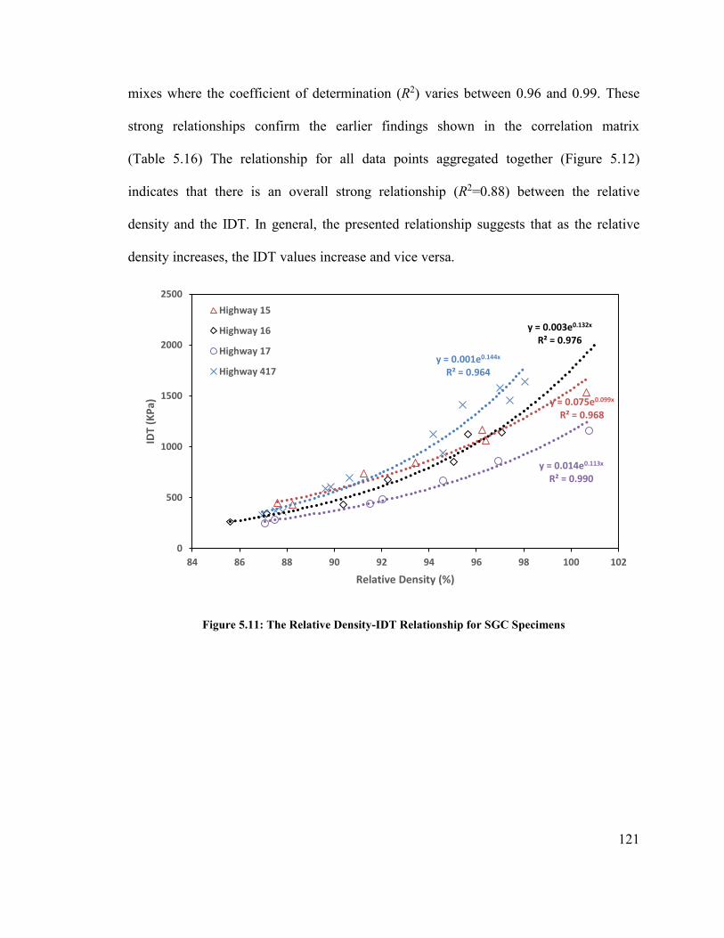
121
mixes where the coefficient of determination (R2) varies between 0.96 and 0.99. These
strong relationships confirm the earlier findings shown in the correlation matrix
(Table 5.16) The relationship for all data points aggregated together (Figure 5.12)
indicates that there is an overall strong relationship (R2=0.88) between the relative
density and the IDT. In general, the presented relationship suggests that as the relative
density increases, the IDT values increase and vice versa.
Figure 5.11: The Relative Density-IDT Relationship for SGC Specimens
y = 0.075e0.099x
R² = 0.968
y = 0.003e0.132x
R² = 0.976
y = 0.014e0.113x
R² = 0.990
y = 0.001e0.144x
R² = 0.964
0
500
1000
1500
2000
2500
84 86 88 90 92 94 96 98 100 102
IDT
(KP
a)
Relative Density (%)
Highway 15
Highway 16
Highway 17
Highway 417
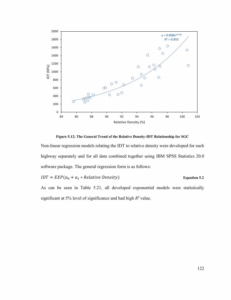
122
Figure 5.12: The General Trend of the Relative Density-IDT Relationship for SGC
Non-linear regression models relating the IDT to relative density were developed for each
highway separately and for all data combined together using IBM SPSS Statistics 20.0
software package. The general regression form is as follows:
𝐼𝐷𝑇 = 𝐸𝑋𝑃(𝑎0 + 𝑎1 ∗ 𝑅𝑒𝑙𝑎𝑡𝑖𝑣𝑒 𝐷𝑒𝑛𝑠𝑖𝑡𝑦) Equation 5.2
As can be seen in Table 5.21, all developed exponential models were statistically
significant at 5% level of significance and had high R2 value.
y = 0.008e0.123x
R² = 0.855
0
200
400
600
800
1000
1200
1400
1600
1800
2000
84 86 88 90 92 94 96 98 100 102
IDT
(KP
a)
Relative Density (%)
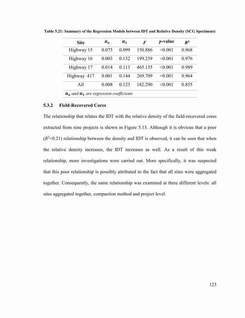
123
Table 5.21: Summary of the Regression Models between IDT and Relative Density (SCG Specimens)
Site 𝒂𝒐 𝒂𝟏 F p-value R2
Highway 15 0.075 0.099 150.886 <0.001 0.968
Highway 16 0.003 0.132 199.239 <0.001 0.976
Highway 17 0.014 0.113 465.135 <0.001 0.989
Highway 417 0.001 0.144 269.709 <0.001 0.964
All 0.008 0.123 182.290 <0.001 0.855
𝒂𝒐 and 𝒂𝟏 are regression coefficients
5.3.2 Field-Recovered Cores
The relationship that relates the IDT with the relative density of the field-recovered cores
extracted from nine projects is shown in Figure 5.13. Although it is obvious that a poor
(R2=0.21) relationship between the density and IDT is observed, it can be seen that when
the relative density increases, the IDT increases as well. As a result of this weak
relationship, more investigations were carried out. More specifically, it was suspected
that this poor relationship is possibly attributed to the fact that all sites were aggregated
together. Consequently, the same relationship was examined at three different levels: all
sites aggregated together, compaction method and project level.
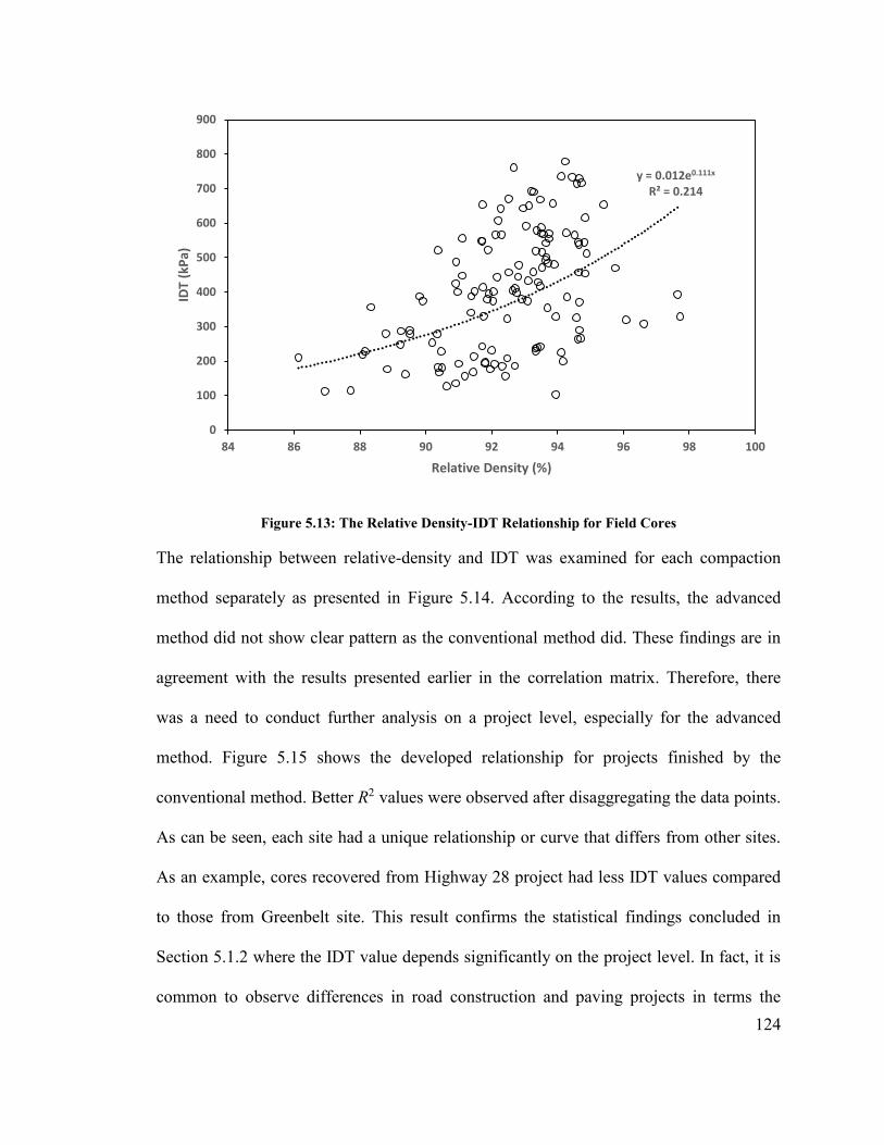
124
Figure 5.13: The Relative Density-IDT Relationship for Field Cores
The relationship between relative-density and IDT was examined for each compaction
method separately as presented in Figure 5.14. According to the results, the advanced
method did not show clear pattern as the conventional method did. These findings are in
agreement with the results presented earlier in the correlation matrix. Therefore, there
was a need to conduct further analysis on a project level, especially for the advanced
method. Figure 5.15 shows the developed relationship for projects finished by the
conventional method. Better R2 values were observed after disaggregating the data points.
As can be seen, each site had a unique relationship or curve that differs from other sites.
As an example, cores recovered from Highway 28 project had less IDT values compared
to those from Greenbelt site. This result confirms the statistical findings concluded in
Section 5.1.2 where the IDT value depends significantly on the project level. In fact, it is
common to observe differences in road construction and paving projects in terms the
y = 0.012e0.111x
R² = 0.214
0
100
200
300
400
500
600
700
800
900
84 86 88 90 92 94 96 98 100
IDT
(kP
a)
Relative Density (%)
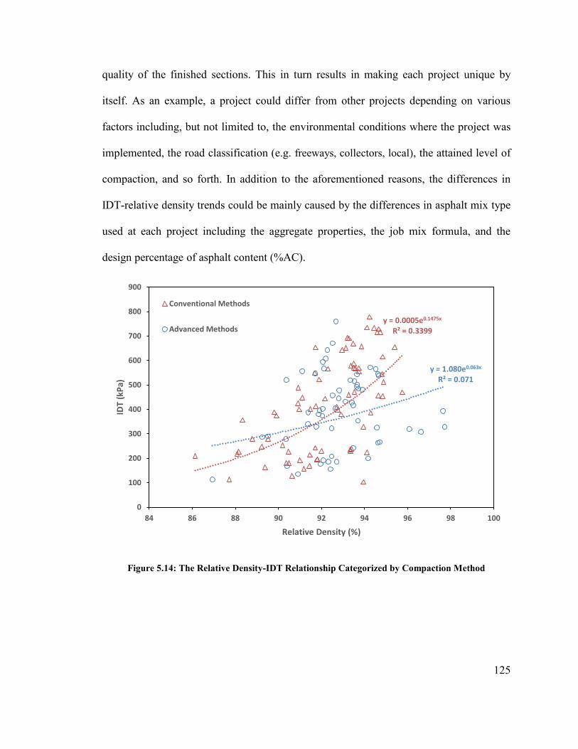
125
quality of the finished sections. This in turn results in making each project unique by
itself. As an example, a project could differ from other projects depending on various
factors including, but not limited to, the environmental conditions where the project was
implemented, the road classification (e.g. freeways, collectors, local), the attained level of
compaction, and so forth. In addition to the aforementioned reasons, the differences in
IDT-relative density trends could be mainly caused by the differences in asphalt mix type
used at each project including the aggregate properties, the job mix formula, and the
design percentage of asphalt content (%AC).
Figure 5.14: The Relative Density-IDT Relationship Categorized by Compaction Method
y = 0.0005e0.1475x
R² = 0.3399
y = 1.080e0.063x
R² = 0.071
0
100
200
300
400
500
600
700
800
900
84 86 88 90 92 94 96 98 100
IDT
(kP
a)
Relative Density (%)
Conventional Methods
Advanced Methods
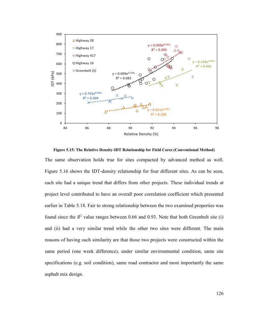
126
Figure 5.15: The Relative Density-IDT Relationship for Field Cores (Conventional Method)
The same observation holds true for sites compacted by advanced method as well.
Figure 5.16 shows the IDT-density relationship for four different sites. As can be seen,
each site had a unique trend that differs from other projects. These individual trends at
project level contributed to have an overall poor correlation coefficient which presented
earlier in Table 5.18. Fair to strong relationship between the two examined properties was
found since the R2 value ranges between 0.66 and 0.93. Note that both Greenbelt site (i)
and (ii) had a very similar trend while the other two sites were different. The main
reasons of having such similarity are that those two projects were constructed within the
same period (one week difference), under similar environmental condition, same site
specifications (e.g. soil condition), same road contractor and most importantly the same
asphalt mix design.
y = 0.011e0.106x
R² = 0.528
y = 0.126e0.087x
R² = 0.442
y = 0.050e0.101x
R² = 0.395
y = 0.009e0.119x
R² = 0.683
y = 0.755e0.065x
R² = 0.569
0
100
200
300
400
500
600
700
800
900
84 86 88 90 92 94 96 98
IDT
(kP
a)
Relative Density (%)
Highway 28
Highway 17
Highway 417
Highway 16
Greenbelt (ii)
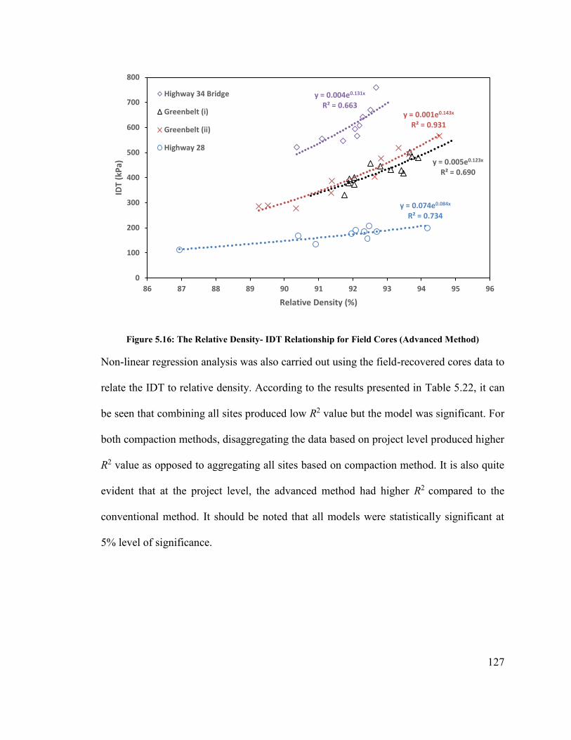
127
Figure 5.16: The Relative Density- IDT Relationship for Field Cores (Advanced Method)
Non-linear regression analysis was also carried out using the field-recovered cores data to
relate the IDT to relative density. According to the results presented in Table 5.22, it can
be seen that combining all sites produced low R2 value but the model was significant. For
both compaction methods, disaggregating the data based on project level produced higher
R2 value as opposed to aggregating all sites based on compaction method. It is also quite
evident that at the project level, the advanced method had higher R2 compared to the
conventional method. It should be noted that all models were statistically significant at
5% level of significance.
y = 0.004e0.131x
R² = 0.663
y = 0.005e0.123x
R² = 0.690
y = 0.001e0.143x
R² = 0.931
y = 0.074e0.084x
R² = 0.734
0
100
200
300
400
500
600
700
800
86 87 88 89 90 91 92 93 94 95 96
IDT
(kP
a)
Relative Density (%)
Highway 34 Bridge
Greenbelt (i)
Greenbelt (ii)
Highway 28
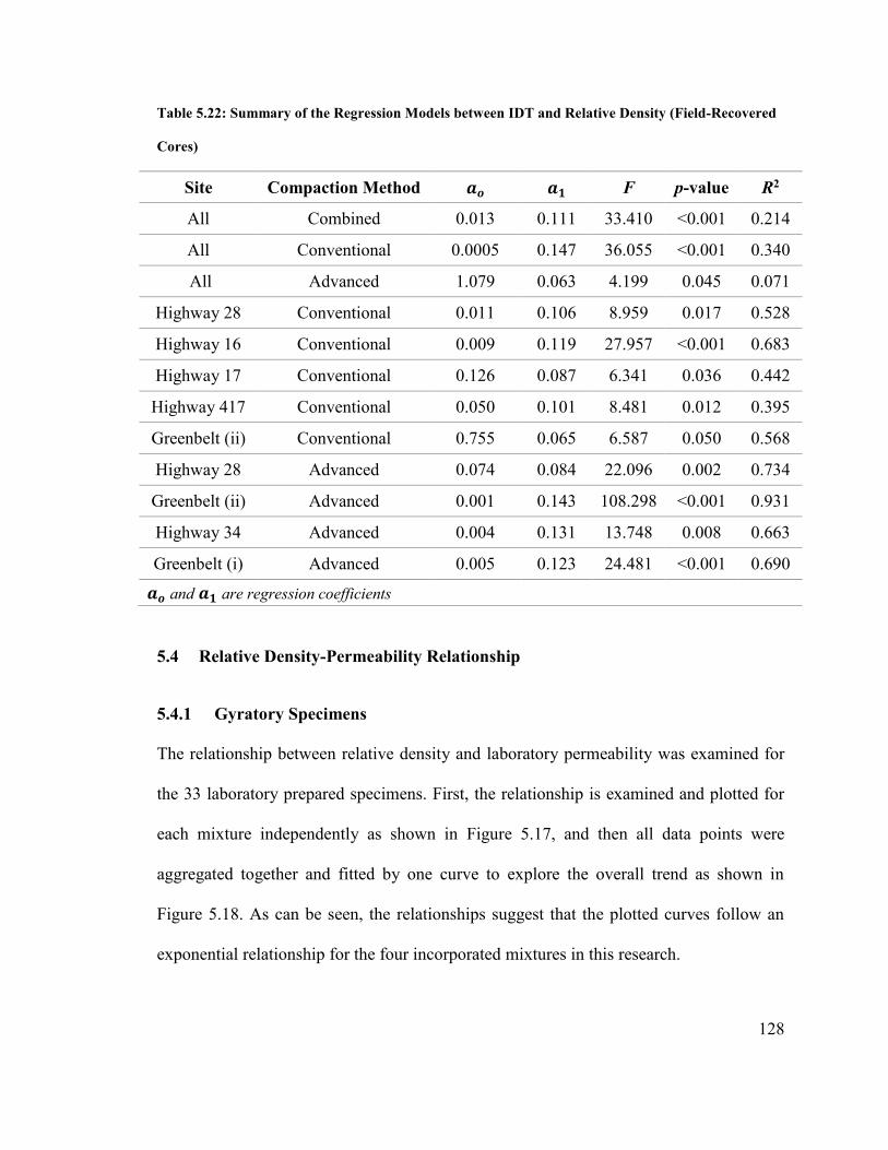
128
Table 5.22: Summary of the Regression Models between IDT and Relative Density (Field-Recovered
Cores)
Site Compaction Method 𝒂𝒐 𝒂𝟏 F p-value R2
All Combined 0.013 0.111 33.410 <0.001 0.214
All Conventional 0.0005 0.147 36.055 <0.001 0.340
All Advanced 1.079 0.063 4.199 0.045 0.071
Highway 28 Conventional 0.011 0.106 8.959 0.017 0.528
Highway 16 Conventional 0.009 0.119 27.957 <0.001 0.683
Highway 17 Conventional 0.126 0.087 6.341 0.036 0.442
Highway 417 Conventional 0.050 0.101 8.481 0.012 0.395
Greenbelt (ii) Conventional 0.755 0.065 6.587 0.050 0.568
Highway 28 Advanced 0.074 0.084 22.096 0.002 0.734
Greenbelt (ii) Advanced 0.001 0.143 108.298 <0.001 0.931
Highway 34 Advanced 0.004 0.131 13.748 0.008 0.663
Greenbelt (i) Advanced 0.005 0.123 24.481 <0.001 0.690
𝒂𝒐 and 𝒂𝟏 are regression coefficients
5.4 Relative Density-Permeability Relationship
5.4.1 Gyratory Specimens
The relationship between relative density and laboratory permeability was examined for
the 33 laboratory prepared specimens. First, the relationship is examined and plotted for
each mixture independently as shown in Figure 5.17, and then all data points were
aggregated together and fitted by one curve to explore the overall trend as shown in
Figure 5.18. As can be seen, the relationships suggest that the plotted curves follow an
exponential relationship for the four incorporated mixtures in this research.
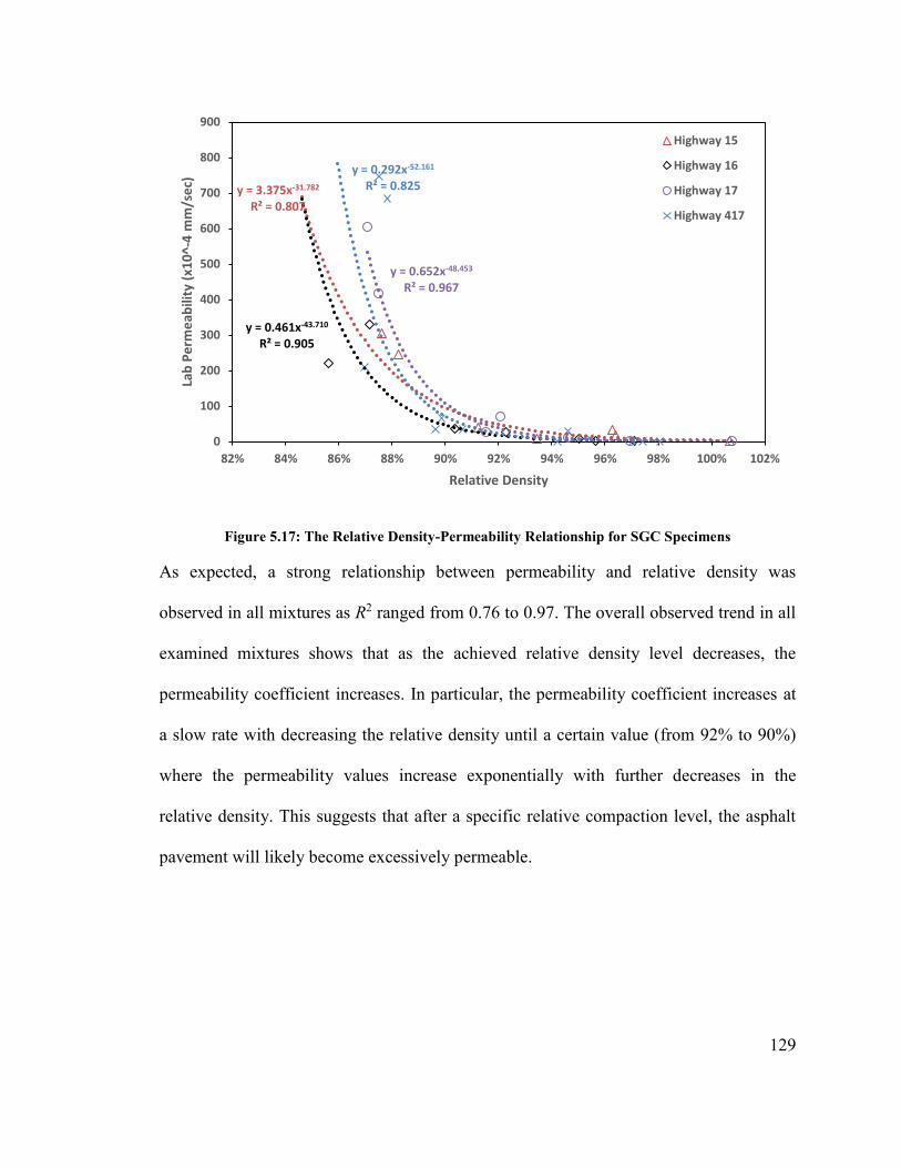
129
Figure 5.17: The Relative Density-Permeability Relationship for SGC Specimens
As expected, a strong relationship between permeability and relative density was
observed in all mixtures as R2 ranged from 0.76 to 0.97. The overall observed trend in all
examined mixtures shows that as the achieved relative density level decreases, the
permeability coefficient increases. In particular, the permeability coefficient increases at
a slow rate with decreasing the relative density until a certain value (from 92% to 90%)
where the permeability values increase exponentially with further decreases in the
relative density. This suggests that after a specific relative compaction level, the asphalt
pavement will likely become excessively permeable.
y = 3.375x-31.782
R² = 0.807
y = 0.461x-43.710
R² = 0.905
y = 0.652x-48.453
R² = 0.967
y = 0.292x-52.161
R² = 0.825
0
100
200
300
400
500
600
700
800
900
82% 84% 86% 88% 90% 92% 94% 96% 98% 100% 102%
Lab
Pe
rme
abili
ty (
x10
^-4
mm
/se
c)
Relative Density
Highway 15
Highway 16
Highway 17
Highway 417
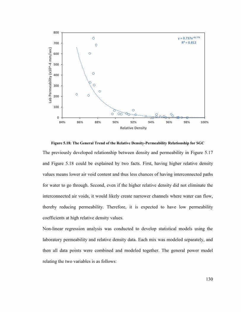
130
Figure 5.18: The General Trend of the Relative Density-Permeability Relationship for SGC
The previously developed relationship between density and permeability in Figure 5.17
and Figure 5.18 could be explained by two facts. First, having higher relative density
values means lower air void content and thus less chances of having interconnected paths
for water to go through. Second, even if the higher relative density did not eliminate the
interconnected air voids, it would likely create narrower channels where water can flow,
thereby reducing permeability. Therefore, it is expected to have low permeability
coefficients at high relative density values.
Non-linear regression analysis was conducted to develop statistical models using the
laboratory permeability and relative density data. Each mix was modeled separately, and
then all data points were combined and modeled together. The general power model
relating the two variables is as follows:
y = 0.737x-43.774
R² = 0.812
0
100
200
300
400
500
600
700
800
84% 86% 88% 90% 92% 94% 96% 98% 100%
Lab
Pe
rme
abili
ty (
x10
^-4
mm
/se
c)
Relative Density

131
𝐿𝑎𝑏 𝑃𝑒𝑟𝑚𝑒𝑎𝑏𝑖𝑙𝑖𝑡𝑦 = 𝑎0 ∗ (𝑅𝑒𝑙𝑎𝑡𝑖𝑣𝑒 𝐷𝑒𝑛𝑠𝑖𝑡𝑦) 𝑎1 Equation 5.3
As can be seen in Table 5.23 , all developed power models were statistically significant
at 5% level of significance and had high R2 value.
Table 5.23: Summary of the Regression Models between Lab Permeability and Relative Density
(SCG Specimens)
Site 𝒂𝟎 𝒂𝟏 F p-value R2
Highway 15 3.371 -31.798 20.945 0.006 0.807
Highway 16 0.461 -43.710 47.489 0.001 0.905
Highway 17 0.651 -48.479 145.175 <0.001 0.967
Highway 417 0.292 -52.163 47.156 <0.001 0.825
All 0.737 -43.781 133.607 <0.001 0.812
𝒂𝒐 and 𝒂𝟏 are regression coefficients
5.4.2 Field-Recovered Cores
The relationship between laboratory permeability and relative density is explored and
presented in Figure 5.19. The results revealed that there is an exponential fair relationship
with (R2 = 0.50) between the laboratory permeability of the field-recovered cores and
relative density. This finding confirms the earlier results developed for the SGC
specimens.
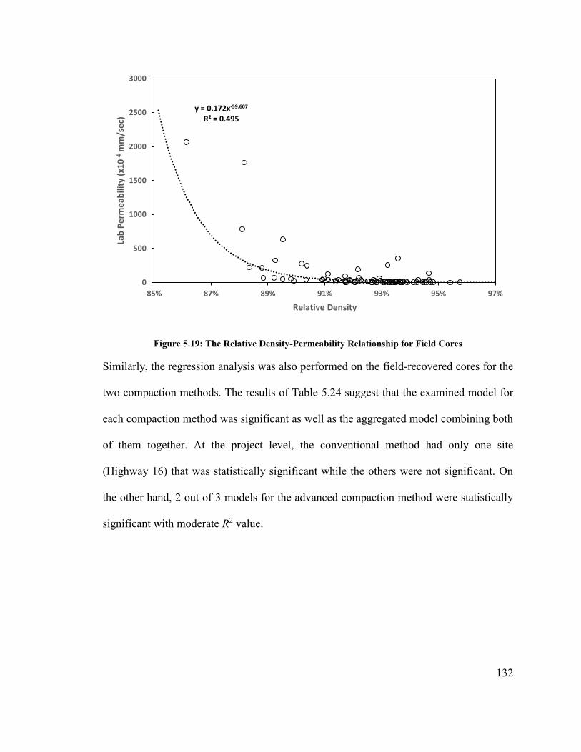
132
Figure 5.19: The Relative Density-Permeability Relationship for Field Cores
Similarly, the regression analysis was also performed on the field-recovered cores for the
two compaction methods. The results of Table 5.24 suggest that the examined model for
each compaction method was significant as well as the aggregated model combining both
of them together. At the project level, the conventional method had only one site
(Highway 16) that was statistically significant while the others were not significant. On
the other hand, 2 out of 3 models for the advanced compaction method were statistically
significant with moderate R2 value.
y = 0.172x-59.607
R² = 0.495
0
500
1000
1500
2000
2500
3000
85% 87% 89% 91% 93% 95% 97%
Lab
Pe
rme
abili
ty (
x10
-4m
m/s
ec)
Relative Density
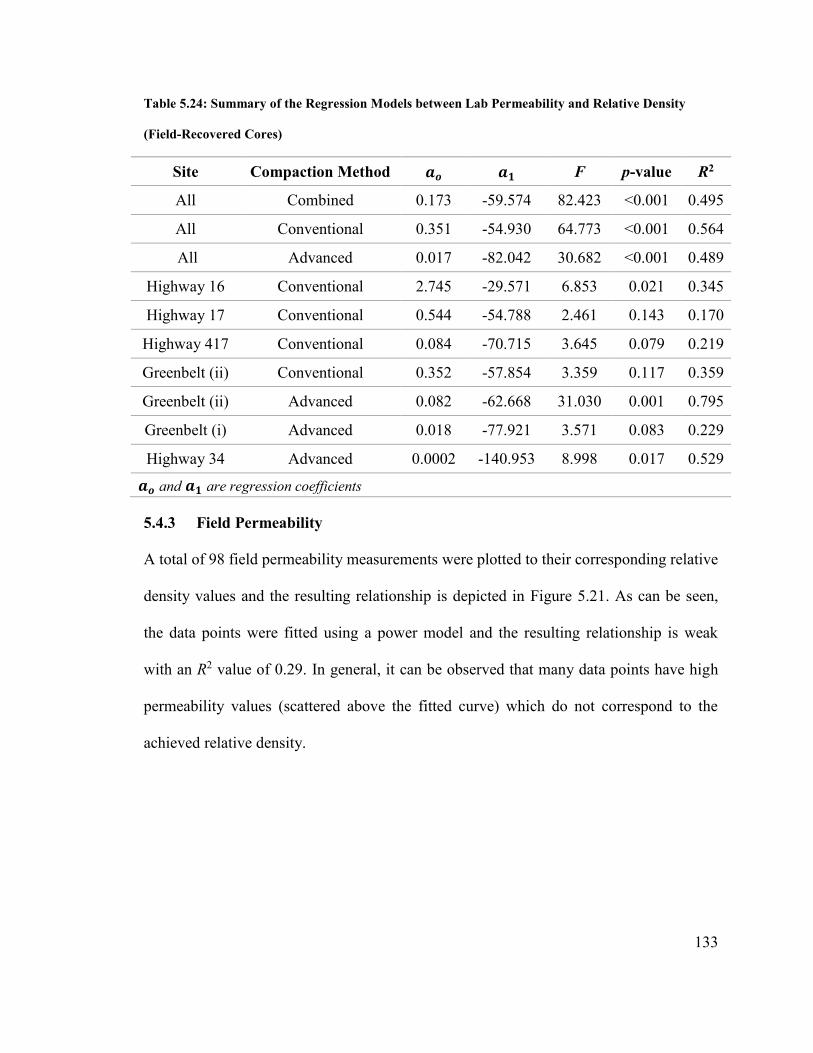
133
Table 5.24: Summary of the Regression Models between Lab Permeability and Relative Density
(Field-Recovered Cores)
Site Compaction Method 𝒂𝒐 𝒂𝟏 F p-value R2
All Combined 0.173 -59.574 82.423 <0.001 0.495
All Conventional 0.351 -54.930 64.773 <0.001 0.564
All Advanced 0.017 -82.042 30.682 <0.001 0.489
Highway 16 Conventional 2.745 -29.571 6.853 0.021 0.345
Highway 17 Conventional 0.544 -54.788 2.461 0.143 0.170
Highway 417 Conventional 0.084 -70.715 3.645 0.079 0.219
Greenbelt (ii) Conventional 0.352 -57.854 3.359 0.117 0.359
Greenbelt (ii) Advanced 0.082 -62.668 31.030 0.001 0.795
Greenbelt (i) Advanced 0.018 -77.921 3.571 0.083 0.229
Highway 34 Advanced 0.0002 -140.953 8.998 0.017 0.529
𝒂𝒐 and 𝒂𝟏 are regression coefficients
5.4.3 Field Permeability
A total of 98 field permeability measurements were plotted to their corresponding relative
density values and the resulting relationship is depicted in Figure 5.21. As can be seen,
the data points were fitted using a power model and the resulting relationship is weak
with an R2 value of 0.29. In general, it can be observed that many data points have high
permeability values (scattered above the fitted curve) which do not correspond to the
achieved relative density.
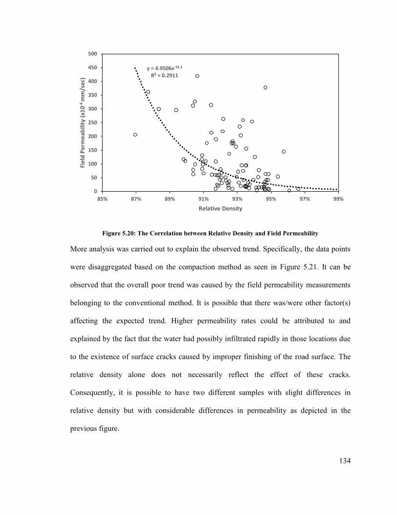
134
Figure 5.20: The Correlation between Relative Density and Field Permeability
More analysis was carried out to explain the observed trend. Specifically, the data points
were disaggregated based on the compaction method as seen in Figure 5.21. It can be
observed that the overall poor trend was caused by the field permeability measurements
belonging to the conventional method. It is possible that there was/were other factor(s)
affecting the expected trend. Higher permeability rates could be attributed to and
explained by the fact that the water had possibly infiltrated rapidly in those locations due
to the existence of surface cracks caused by improper finishing of the road surface. The
relative density alone does not necessarily reflect the effect of these cracks.
Consequently, it is possible to have two different samples with slight differences in
relative density but with considerable differences in permeability as depicted in the
previous figure.
y = 4.9506x-32.2
R² = 0.2911
0
50
100
150
200
250
300
350
400
450
500
85% 87% 89% 91% 93% 95% 97% 99%
Fie
ld P
erm
eab
ility
(x1
0-4
mm
/se
c)
Relative Density
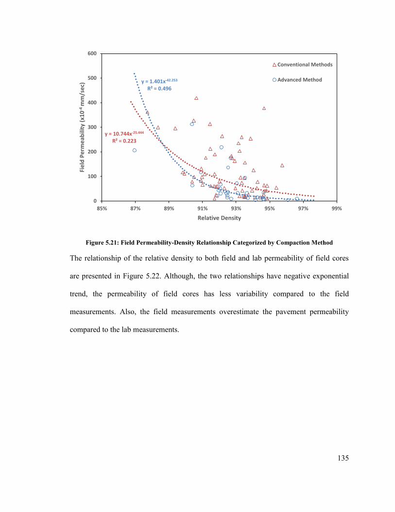
135
Figure 5.21: Field Permeability-Density Relationship Categorized by Compaction Method
The relationship of the relative density to both field and lab permeability of field cores
are presented in Figure 5.22. Although, the two relationships have negative exponential
trend, the permeability of field cores has less variability compared to the field
measurements. Also, the field measurements overestimate the pavement permeability
compared to the lab measurements.
y = 10.744x-25.444
R² = 0.223
y = 1.401x-42.253
R² = 0.496
0
100
200
300
400
500
600
85% 87% 89% 91% 93% 95% 97% 99%
Fie
ld P
erm
eab
ility
(x1
0-4
mm
/se
c)
Relative Density
Conventional Methods
Advanced Method

136
Figure 5.22: The Relative Density-Permeability Trend for Field Cores and Field Measurements
The relative density was used as independent variable while the field permeability was
used as the dependent variable in the regression analysis. The following equation
describes the general form of the power model:
𝐹𝑖𝑒𝑙𝑑 𝑃𝑒𝑟𝑚𝑒𝑎𝑏𝑖𝑙𝑖𝑡𝑦 = 𝑎0 ∗ (𝑅𝑒𝑙𝑎𝑡𝑖𝑣𝑒 𝐷𝑒𝑛𝑠𝑖𝑡𝑦) 𝑎1 Equation 5.4
The models summarized in Table 5.25 suggest that aggregating the data points based on
compaction method as well as combining the two compaction methods produced
significant models. In general, building individual models at the project level was not
statistically significant for the two compaction methods.
y = 4.951x-32.196
R² = 0.291
y = 0.172x-59.607
R² = 0.495
0
100
200
300
400
500
600
700
800
900
1000
84% 86% 88% 90% 92% 94% 96% 98% 100%
Pe
rme
abili
ty (
x10
-4m
m/s
ec)
Relative Density
Field Permeability
Lab Permeability on Field Cores
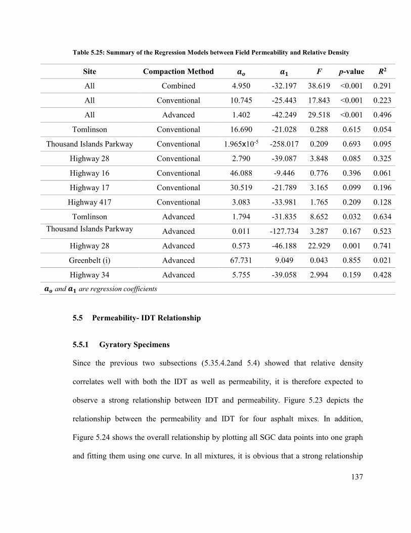
137
Table 5.25: Summary of the Regression Models between Field Permeability and Relative Density
Site Compaction Method 𝒂𝒐 𝒂𝟏 F p-value R2
All Combined 4.950 -32.197 38.619 <0.001 0.291
All Conventional 10.745 -25.443 17.843 <0.001 0.223
All Advanced 1.402 -42.249 29.518 <0.001 0.496
Tomlinson Conventional 16.690 -21.028 0.288 0.615 0.054
Thousand Islands Parkway Conventional 1.965x10⁻⁵ -258.017 0.209 0.693 0.095
Highway 28 Conventional 2.790 -39.087 3.848 0.085 0.325
Highway 16 Conventional 46.088 -9.446 0.776 0.396 0.061
Highway 17 Conventional 30.519 -21.789 3.165 0.099 0.196
Highway 417 Conventional 3.083 -33.981 1.765 0.209 0.128
Tomlinson Advanced 1.794 -31.835 8.652 0.032 0.634
Thousand Islands Parkway
Advanced 0.011 -127.734 3.287 0.167 0.523
Highway 28 Advanced 0.573 -46.188 22.929 0.001 0.741
Greenbelt (i) Advanced 67.731 9.049 0.043 0.855 0.021
Highway 34 Advanced 5.755 -39.058 2.994 0.159 0.428
𝒂𝒐 and 𝒂𝟏 are regression coefficients
5.5 Permeability- IDT Relationship
5.5.1 Gyratory Specimens
Since the previous two subsections (5.35.4.2and 5.4) showed that relative density
correlates well with both the IDT as well as permeability, it is therefore expected to
observe a strong relationship between IDT and permeability. Figure 5.23 depicts the
relationship between the permeability and IDT for four asphalt mixes. In addition,
Figure 5.24 shows the overall relationship by plotting all SGC data points into one graph
and fitting them using one curve. In all mixtures, it is obvious that a strong relationship
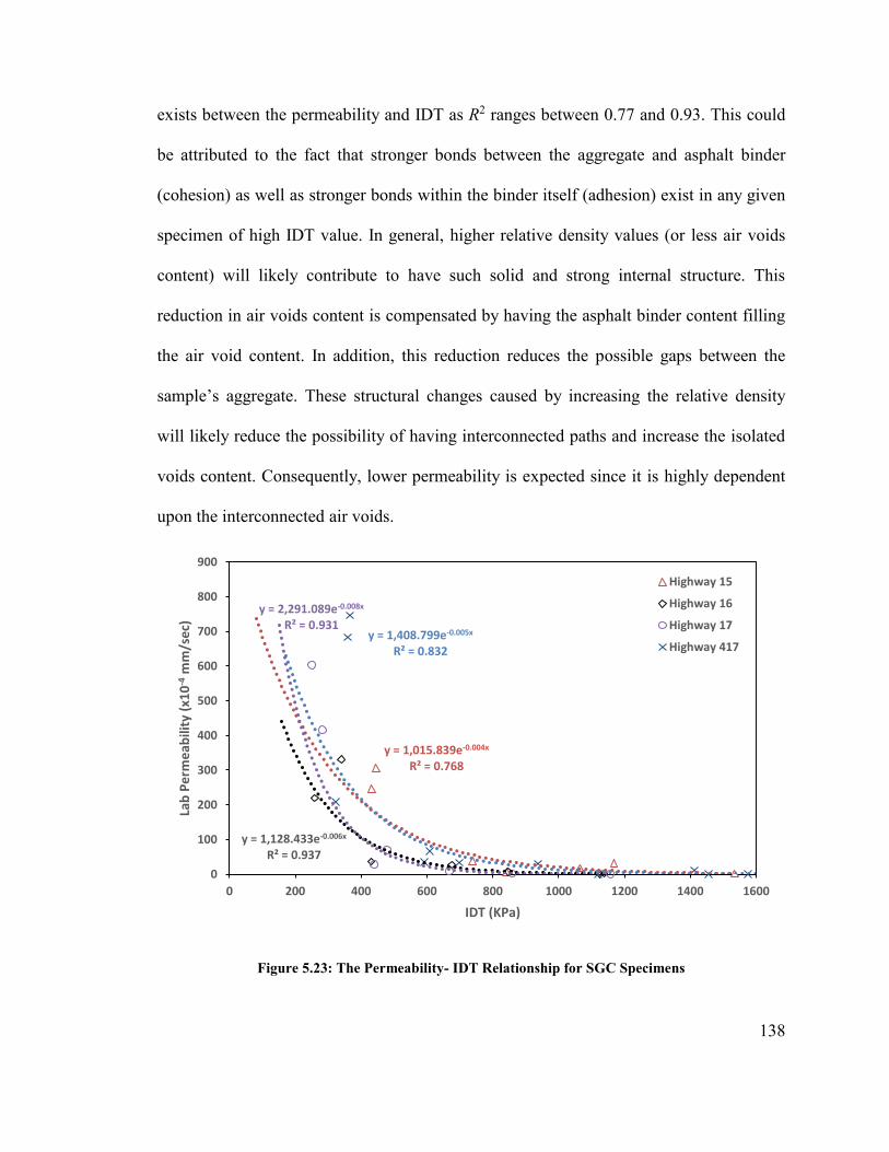
138
exists between the permeability and IDT as R2 ranges between 0.77 and 0.93. This could
be attributed to the fact that stronger bonds between the aggregate and asphalt binder
(cohesion) as well as stronger bonds within the binder itself (adhesion) exist in any given
specimen of high IDT value. In general, higher relative density values (or less air voids
content) will likely contribute to have such solid and strong internal structure. This
reduction in air voids content is compensated by having the asphalt binder content filling
the air void content. In addition, this reduction reduces the possible gaps between the
sample’s aggregate. These structural changes caused by increasing the relative density
will likely reduce the possibility of having interconnected paths and increase the isolated
voids content. Consequently, lower permeability is expected since it is highly dependent
upon the interconnected air voids.
Figure 5.23: The Permeability- IDT Relationship for SGC Specimens
y = 1,015.839e-0.004x
R² = 0.768
y = 1,128.433e-0.006x
R² = 0.937
y = 2,291.089e-0.008x
R² = 0.931y = 1,408.799e-0.005x
R² = 0.832
0
100
200
300
400
500
600
700
800
900
0 200 400 600 800 1000 1200 1400 1600
Lab
Pe
rme
abili
ty (
x10
-4m
m/s
ec)
IDT (KPa)
Highway 15
Highway 16
Highway 17
Highway 417
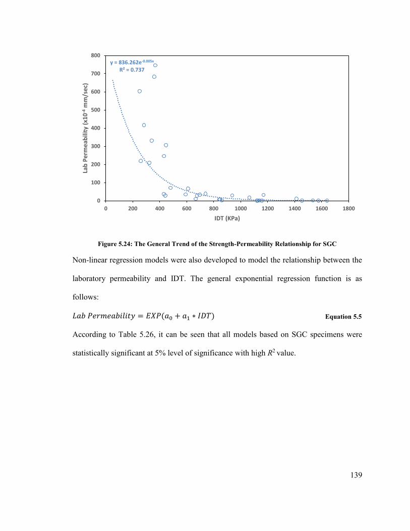
139
Figure 5.24: The General Trend of the Strength-Permeability Relationship for SGC
Non-linear regression models were also developed to model the relationship between the
laboratory permeability and IDT. The general exponential regression function is as
follows:
𝐿𝑎𝑏 𝑃𝑒𝑟𝑚𝑒𝑎𝑏𝑖𝑙𝑖𝑡𝑦 = 𝐸𝑋𝑃(𝑎0 + 𝑎1 ∗ 𝐼𝐷𝑇) Equation 5.5
According to Table 5.26, it can be seen that all models based on SGC specimens were
statistically significant at 5% level of significance with high R2 value.
y = 836.262e-0.005x
R² = 0.737
0
100
200
300
400
500
600
700
800
0 200 400 600 800 1000 1200 1400 1600 1800
Lab
Pe
rme
abili
ty (
x10
-4m
m/s
ec)
IDT (KPa)

140
Table 5.26: Summary of the Regression Models between Lab Permeability and IDT (SCG
Specimens)
Site 𝒂𝒐 𝒂𝟏 F p-value R2
Highway 15 1015.851 -0.004 16.558 0.010 0.768
Highway 16 1128.440 -0.006 74.724 <0.001 0.937
Highway 17 2291.183 -0.008 67.582 <0.001 0.931
Highway 417 1408.806 -0.005 49.537 <0.001 0.832
All 836.270 -0.005 86.679 <0.001 0.737
𝒂𝒐 and 𝒂𝟏 are regression coefficients
5.5.2 Field-Recovered Cores
Similar to Section 5.3.2, the relationship between IDT and lab permeability was
investigated at the same three different levels introduced earlier. Figure 5.25 shows the
overall trend when aggregating all data points. A moderate relationship (R2 = 0.43) was
observed at this level of classification. The next level of analysis categorized by
compaction method was then performed and the results are presented in Figure 5.26. A
fair relationship was observed for results obtained and finished by the conventional
method while the advanced method showed variability in the data with low coefficient of
determination.
The relationship between permeability and IDT was also inspected site-by-site which is
the third level of analysis. Figure 5.27 presents the results of conventional compaction
method. A logarithmic scale was used to represent the lab permeability due to the
existence of some high permeability values. In general, fair to strong relationship (0.33 <
R2 < 0.83) exists between the IDT and laboratory permeability and it is best fitted by an
exponential curve. This confirms the finding obtained by the SGC specimens when
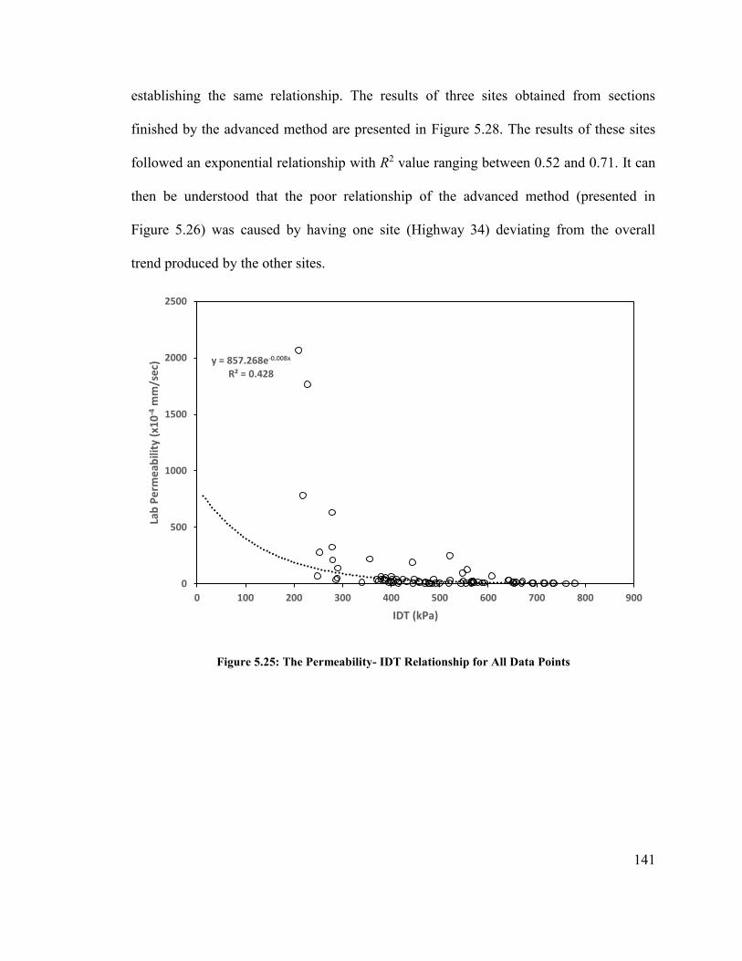
141
establishing the same relationship. The results of three sites obtained from sections
finished by the advanced method are presented in Figure 5.28. The results of these sites
followed an exponential relationship with R2 value ranging between 0.52 and 0.71. It can
then be understood that the poor relationship of the advanced method (presented in
Figure 5.26) was caused by having one site (Highway 34) deviating from the overall
trend produced by the other sites.
Figure 5.25: The Permeability- IDT Relationship for All Data Points
y = 857.268e-0.008x
R² = 0.428
0
500
1000
1500
2000
2500
0 100 200 300 400 500 600 700 800 900
Lab
Pe
rme
abili
ty (
x10
-4m
m/s
ec)
IDT (kPa)
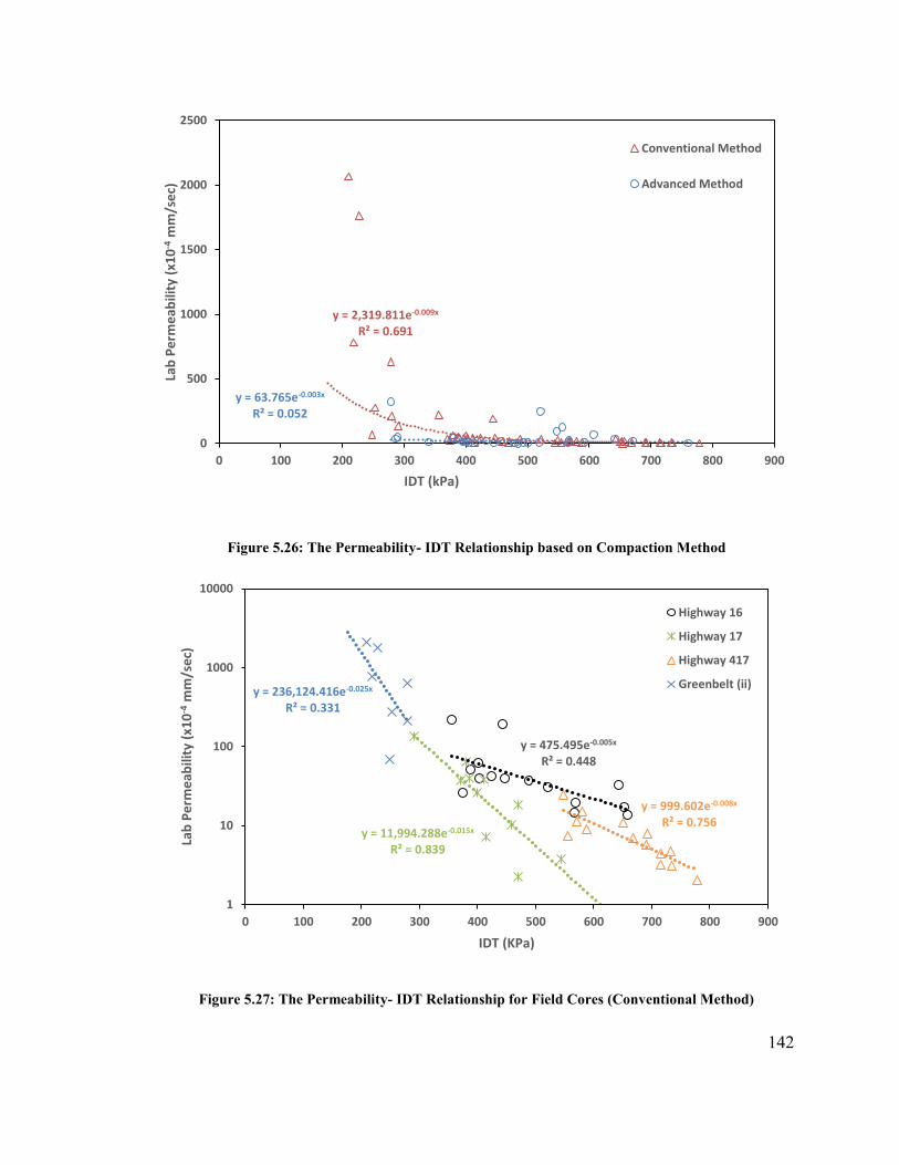
142
Figure 5.26: The Permeability- IDT Relationship based on Compaction Method
Figure 5.27: The Permeability- IDT Relationship for Field Cores (Conventional Method)
y = 2,319.811e-0.009x
R² = 0.691
y = 63.765e-0.003x
R² = 0.052
0
500
1000
1500
2000
2500
0 100 200 300 400 500 600 700 800 900
Lab
Pe
rme
abili
ty (
x10
-4m
m/s
ec)
IDT (kPa)
Conventional Method
Advanced Method
y = 475.495e-0.005x
R² = 0.448
y = 11,994.288e-0.015x
R² = 0.839
y = 999.602e-0.008x
R² = 0.756
y = 236,124.416e-0.025x
R² = 0.331
1
10
100
1000
10000
0 100 200 300 400 500 600 700 800 900
Lab
Pe
rme
abili
ty (
x10
-4m
m/s
ec)
IDT (KPa)
Highway 16
Highway 17
Highway 417
Greenbelt (ii)

143
Figure 5.28: The Permeability- IDT Relationship for Field Cores (Advanced Method)
It was concluded in the literature review (Chapter 2) of this thesis that the permeability of
HMA is highly affected by the NMAS when examining the permeability-density
relationship. In other words, the permeability-density trend of road sections having 12.5
mm NMAS is different from roads with 19mm NMAS. It is important to mention that all
incorporated sites in this study have a NMAS of 12.5mm. The previously developed
relationships (Figure 5.15, Figure 5.16, Figure 5.27 and Figure 5.28) suggest that, unlike
the permeability-density relationship, unique strength-density or strength-permeability
relationships could exist for the same NMAS. This is possibly attributed to the
differences in asphalt mixtures used in each project.
The regression analysis presented in Table 5.27 implies that the developed model for the
conventional method was statistically significant while the advanced was not. It is
important to mention that there are slight differences in the regression coefficients
y = 192,596.508e-0.023x
R² = 0.496
y = 1,254.955e-0.011x
R² = 0.674
y = 1,142,825.447e-0.017x
R² = 0.714
1
10
100
1000
0 100 200 300 400 500 600 700 800
Lab
Pe
rme
abili
ty (
x10
-4m
m/s
ec)
IDT (KPa)
Greenbelt (i)
Greenbelt (ii)
Highway 34 Bridge
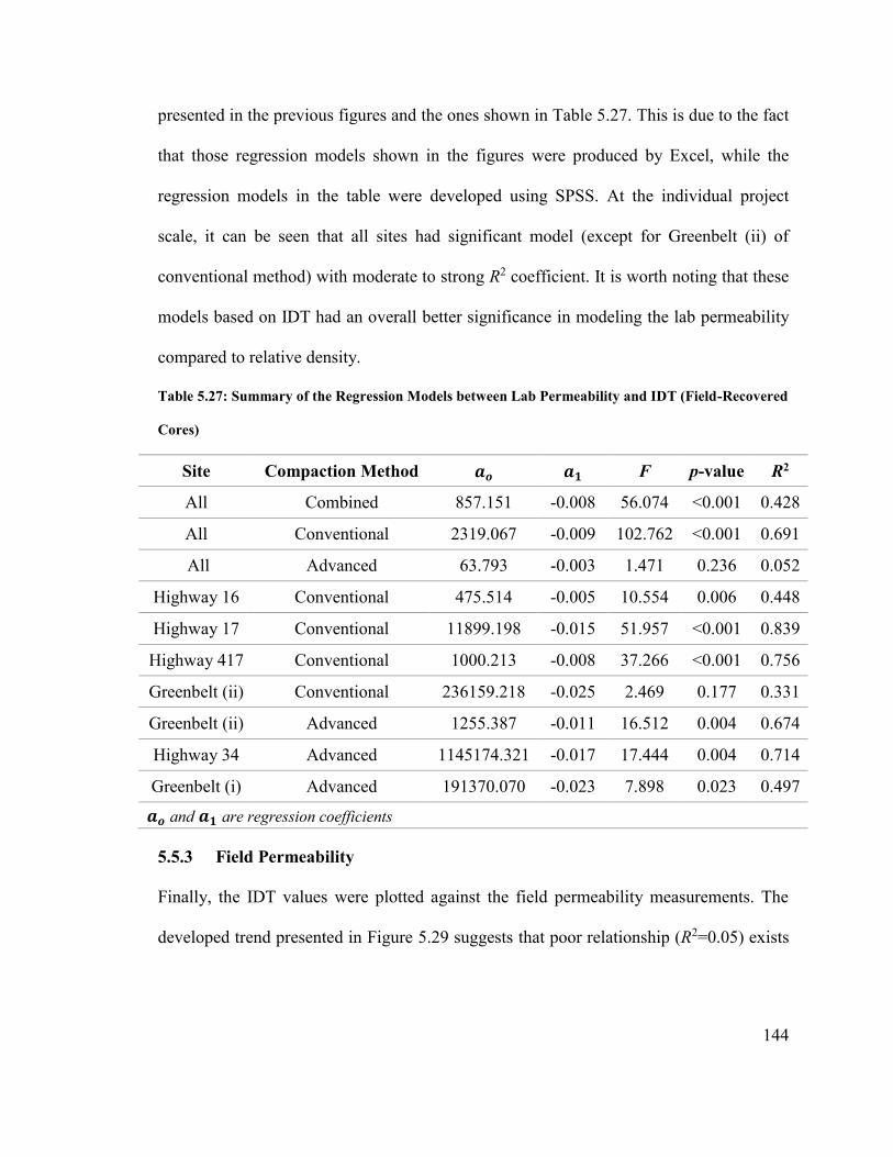
144
presented in the previous figures and the ones shown in Table 5.27. This is due to the fact
that those regression models shown in the figures were produced by Excel, while the
regression models in the table were developed using SPSS. At the individual project
scale, it can be seen that all sites had significant model (except for Greenbelt (ii) of
conventional method) with moderate to strong R2 coefficient. It is worth noting that these
models based on IDT had an overall better significance in modeling the lab permeability
compared to relative density.
Table 5.27: Summary of the Regression Models between Lab Permeability and IDT (Field-Recovered
Cores)
Site Compaction Method 𝒂𝒐 𝒂𝟏 F p-value R2
All Combined 857.151 -0.008 56.074 <0.001 0.428
All Conventional 2319.067 -0.009 102.762 <0.001 0.691
All Advanced 63.793 -0.003 1.471 0.236 0.052
Highway 16 Conventional 475.514 -0.005 10.554 0.006 0.448
Highway 17 Conventional 11899.198 -0.015 51.957 <0.001 0.839
Highway 417 Conventional 1000.213 -0.008 37.266 <0.001 0.756
Greenbelt (ii) Conventional 236159.218 -0.025 2.469 0.177 0.331
Greenbelt (ii) Advanced 1255.387 -0.011 16.512 0.004 0.674
Highway 34 Advanced 1145174.321 -0.017 17.444 0.004 0.714
Greenbelt (i) Advanced 191370.070 -0.023 7.898 0.023 0.497
𝒂𝒐 and 𝒂𝟏 are regression coefficients
5.5.3 Field Permeability
Finally, the IDT values were plotted against the field permeability measurements. The
developed trend presented in Figure 5.29 suggests that poor relationship (R2=0.05) exists
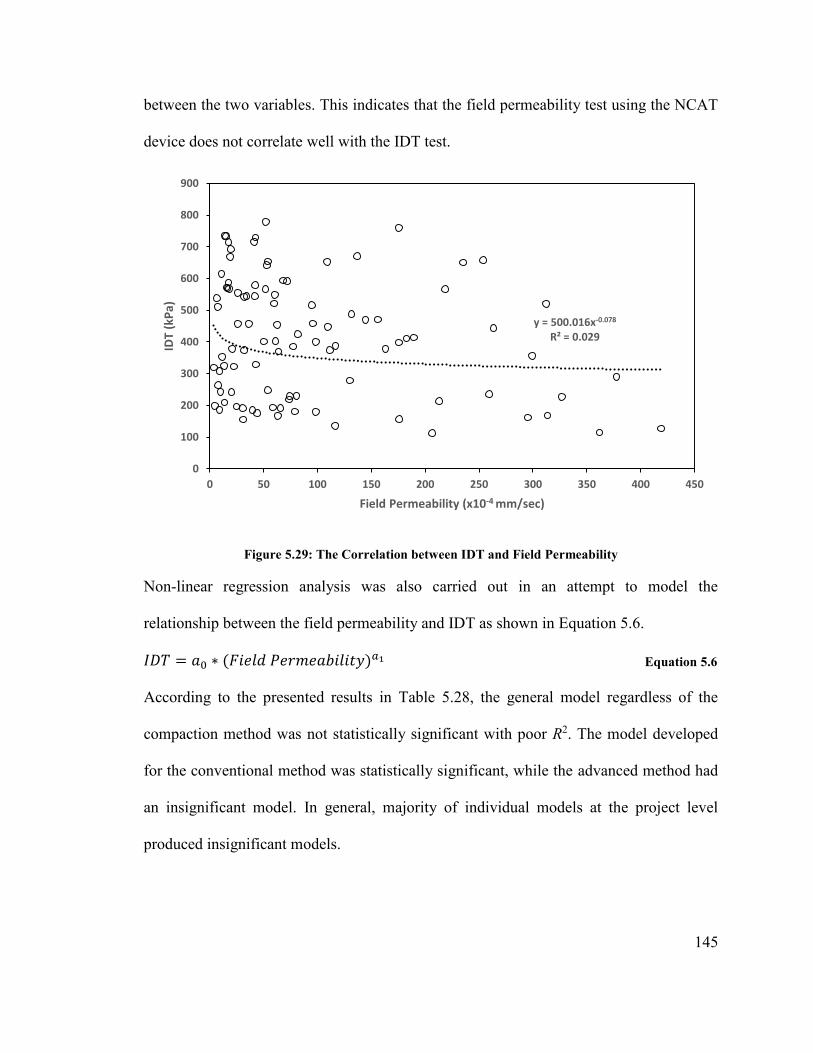
145
between the two variables. This indicates that the field permeability test using the NCAT
device does not correlate well with the IDT test.
Figure 5.29: The Correlation between IDT and Field Permeability
Non-linear regression analysis was also carried out in an attempt to model the
relationship between the field permeability and IDT as shown in Equation 5.6.
𝐼𝐷𝑇 = 𝑎0 ∗ (𝐹𝑖𝑒𝑙𝑑 𝑃𝑒𝑟𝑚𝑒𝑎𝑏𝑖𝑙𝑖𝑡𝑦)𝑎1 Equation 5.6
According to the presented results in Table 5.28, the general model regardless of the
compaction method was not statistically significant with poor R2. The model developed
for the conventional method was statistically significant, while the advanced method had
an insignificant model. In general, majority of individual models at the project level
produced insignificant models.
y = 500.016x-0.078
R² = 0.029
0
100
200
300
400
500
600
700
800
900
0 50 100 150 200 250 300 350 400 450
IDT
(kP
a)
Field Permeability (x10-4 mm/sec)
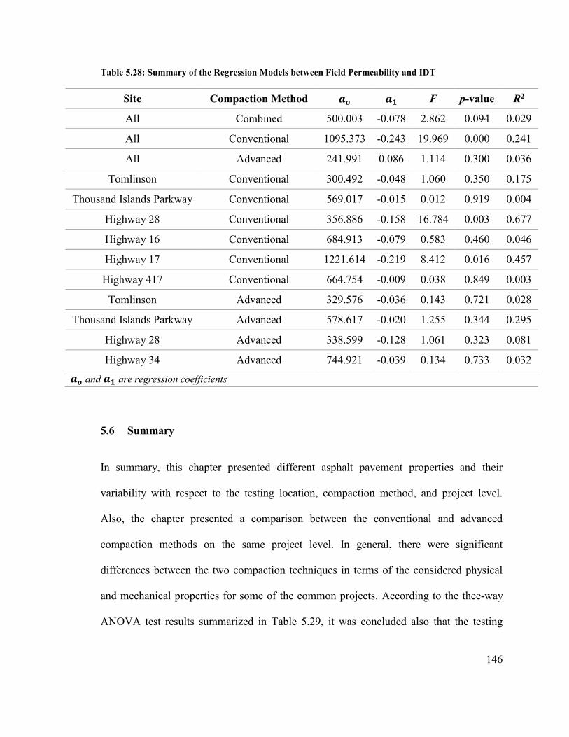
146
Table 5.28: Summary of the Regression Models between Field Permeability and IDT
Site Compaction Method 𝒂𝒐 𝒂𝟏 F p-value R2
All Combined 500.003 -0.078 2.862 0.094 0.029
All Conventional 1095.373 -0.243 19.969 0.000 0.241
All Advanced 241.991 0.086 1.114 0.300 0.036
Tomlinson Conventional 300.492 -0.048 1.060 0.350 0.175
Thousand Islands Parkway Conventional 569.017 -0.015 0.012 0.919 0.004
Highway 28 Conventional 356.886 -0.158 16.784 0.003 0.677
Highway 16 Conventional 684.913 -0.079 0.583 0.460 0.046
Highway 17 Conventional 1221.614 -0.219 8.412 0.016 0.457
Highway 417 Conventional 664.754 -0.009 0.038 0.849 0.003
Tomlinson Advanced 329.576 -0.036 0.143 0.721 0.028
Thousand Islands Parkway Advanced 578.617 -0.020 1.255 0.344 0.295
Highway 28 Advanced 338.599 -0.128 1.061 0.323 0.081
Highway 34 Advanced 744.921 -0.039 0.134 0.733 0.032
𝒂𝒐 and 𝒂𝟏 are regression coefficients
5.6 Summary
In summary, this chapter presented different asphalt pavement properties and their
variability with respect to the testing location, compaction method, and project level.
Also, the chapter presented a comparison between the conventional and advanced
compaction methods on the same project level. In general, there were significant
differences between the two compaction techniques in terms of the considered physical
and mechanical properties for some of the common projects. According to the thee-way
ANOVA test results summarized in Table 5.29, it was concluded also that the testing
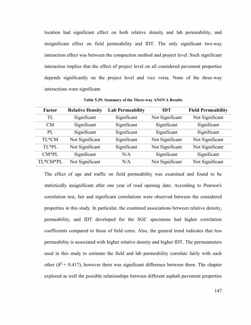
147
location had significant effect on both relative density and lab permeability, and
insignificant effect on field permeability and IDT. The only significant two-way
interaction effect was between the compaction method and project level. Such significant
interaction implies that the effect of project level on all considered pavement properties
depends significantly on the project level and vice versa. None of the three-way
interactions were significant.
Table 5.29: Summary of the Three-way ANOVA Results
Factor Relative Density Lab Permeability IDT Field Permeability
TL Significant Significant Not Significant Not Significant
CM Significant Significant Significant Significant
PL Significant Significant Significant Significant
TL*CM Not Significant Significant Not Significant Not Significant
TL*PL Not Significant Significant Not Significant Not Significant
CM*PL Significant N/A Significant Significant
TL*CM*PL Not Significant N/A Not Significant Not Significant
The effect of age and traffic on field permeability was examined and found to be
statistically insignificant after one year of road opening date. According to Pearson's
correlation test, fair and significant correlations were observed between the considered
properties in this study. In particular, the examined associations between relative density,
permeability, and IDT developed for the SGC specimens had higher correlation
coefficients compared to those of field cores. Also, the general trend indicates that less
permeability is associated with higher relative density and higher IDT. The permeameters
used in this study to estimate the field and lab permeability correlate fairly with each
other (R2 = 0.417), however there was significant difference between them. The chapter
explored as well the possible relationships between different asphalt pavement properties
148
in two different settings; the field and lab. The relationships between field permeability
and any of the three laboratory tests (permeability, density, and IDT) were generally
moderate to poor. The chapter also presented the results of non-linear regression analysis
between the different dependent and independent variables. In general, all models based
on SGC specimens were statistically significant with high R2 coefficient. For the field-
recovered cores, it was found that modeling the lab permeability based on IDT is better
than modeling it using the relative density at project level. Neither the relative density nor
the IDT were able to show significance in modeling the field permeability at the project
level. In most cases, aggregating the data points based on the compaction method showed
significant model, but poor R2 coefficient.
149
CHAPTER 6: CONCLUSIONS AND
RECOMMENDATIONS
6.1 Summary
Ensuring the highest possible qualities of the finished asphalt roads is essential to
minimize various types of damage in the short and long terms of the service life of the
pavement. This research was designed and carried out to examine a more reliable
pavement characteristic or test method based on permeability to evaluate the as-built
quality of the newly HMA road pavements. This is because permeability is closely
related to moisture-induced damages more than relative density, the currently adopted
pavement characteristic by road authorities.
The first step towards achieving the research objectives was to carry out a comprehensive
review of the state of the art concerning the methods and techniques used to estimate both
the in-situ and laboratory permeability. Based on this review, the NCAT and the Karol-
Warner permeameters were selected for performing the field and laboratory permeability
test respectively.
The research scope was limited to particular sites in Eastern Ontario, most of which were
selected in consultation with engineers from MTO whilst other sections were built as in-
house field trials intended to evaluate asphalt mixtures compacted using the AMIR-II
compactor. In addition, different asphalt mixture types corresponding to the same
mixtures studied in the field were provided by the MTO for the purpose of performing
the required laboratory experiments. The field and laboratory investigations were
performed on newly constructed sites as well as other one year in-service sections. The
150
field experimental program entailed performing the in-situ permeability testing in
addition to recovering field cores from the exact testing location where the field
permeability was conducted. The laboratory testing program consisted of various
laboratory tests including relative density, lab permeability, and IDT. The
aforementioned laboratory tests were carried out on both the field-recovered cores as well
as the laboratory prepared specimens by the SGC.
The variability of the mechanical and physical properties was examined against three
different factors. Those variability were described in terms of the relative density, IDT,
field and lab permeability. The first factor was the testing location which was determined
by performing the field permeability as well as core sampling at five different locations in
the asphalt mat. The effect of the compaction technique on HMA properties was
addressed and included in this research as the second factor. Particularly, the current
compaction method including the conventional vibratory steel drum and pneumatic train
rollers were compared to the advanced method. The last factor was termed as the project
level in which the effect of project type on the HMA properties was examined. The three-
way ANOVA test was select to examine the possible effects of all these three factors on
each pavement property separately.
In addition to examining the permeability characteristic of HMA for the purpose of
utilizing it as reliable test method, a comprehensive analysis was performed on the data
and results to understand the interactions between the physical and mechanical properties
of HMA asphalt pavements. More specifically, the relationship between the permeability
of HMA and other important asphalt pavement properties (relative density and IDT) was
151
studied in this research to examine the validity of proposing the permeability in addition
to the density to improve the reliability of the current QA/QC techniques adopted by road
authorities. Several conclusions, findings, and recommendations were drawn on the basis
of the carried analysis.
6.2 Conclusions
According to the conducted research, the following can be concluded:
1) The current quality criteria which depend only on the measurement of the relative
densities of finished pavements in the field may not be sufficient to decide on the
quality of the finished pavement. The results of this research provided evidence
based on laboratory and field measurements pointing to the fact that
measurements of lab permeability along with the relative density must be
considered and added to the mix design specifications.
2) Based on the results of measuring the IDT of field-recovered cores and SGC
specimens, it is quite evident that considering both the permeability and relative
density of the designed mix provide a better indication of the actual physical
condition of newly constructed HMA road pavements which in turn reflects the
expected long-term performance. This result is further validated and supported
through several field and laboratory observations of the selected test roads.
3) Laboratory investigations based on SGC specimens showed that there is a strong
exponential relationship between the laboratory permeability and the relative
density. This finding was further supported and confirmed when the relationship
between lab permeability and IDT was constructed. In general, the relationship
152
suggests that higher permeability is highly related to both less relative density and
less IDT.
4) The relationship between lab permeability and relative density based on the field-
recovered cores had fair relationship. When relating the lab permeability to IDT,
strong relationship was also found.
5) The field permeability exhibited poor relationship to both the relative density.
This finding was confirmed when the relationship between the field permeability
and IDT was examined since the resulting trend was poor as well. Therefore, it
was concluded that other factor(s) might have affected the trend as the variability
in field permeability could not be explained by neither the relative density nor the
IDT. Since majority of the used data were collected from newly constructed
roads, it means that effect of ageing or traffic did not contribute to this poor trend
and these factors could be eliminated. The reason might be attributed to the
construction method used to build these new road pavements, the existence of
construction induced-cracks (hairline cracks perpendicular to the rolling direction
of field compactors), the non-uniform or heterogeneous distribution of air voids in
the field, the anisotropic nature of water flow in field, or combination of any of
these factors. Having some field measurements incorporating these shortages can
significantly contribute to produce inconsistency in the overall trend.
6) The field permeability estimated using the NCAT field permeameter exhibited
generally fair relationship to the lab permeability using Karol-Warner
permeameter. It was concluded also that the field permeability has higher
inconsistency and overestimates pavement permeability. This was attributed
153
mainly to the multiple flow directions of water in the field, compared to the one
dimensional flow of water in the lab.
7) The regression models relating permeability to both relative density and IDT
based on SGC specimens were statistically significant with strong R2 coefficient.
For the field-recovered cores, it was found that majority of the regression models
developed to model the lab permeability based on the IDT values were
statistically significant compared to models based on relative density. The
regression analysis revealed that it is not possible to model the field permeability
based laboratory measurements represented by the relative density and IDT.
8) According to the three-way ANOVA test results, it was concluded that in all
pavement properties (except for lab permeability due to inapplicability and dataset
limitations) there was insignificant three-way interaction effect between the three
considered factors. The only statistically significant two-way interaction was
between the compaction method and project level. This implies that the effect of
the compaction method on field permeability, relative density, or IDT depends
significantly on the project level and vice versa. The effect of testing location was
significant for the relative density and lab permeability only, while it was
insignificant when examining the IDT and the field permeability.
9) There was a significant difference between the two compaction techniques when
studying and comparing some of the selected sites where the two compactors
were used side-by-side under the same conditions. In terms of both field and lab
permeability values, the advanced method provided less permeable sections of
HMA asphalt pavement. Also, the advanced method showed higher IDT and
154
relative density values as opposed to the current compaction method. All these
differences in terms of the four considered pavement properties in this study were
statistically significant.
6.3 Recommendations for Future Studies
The research scope had several constrains including the type of asphalt mixture as 12.5
mm, pavement mix type as dense-graded HMA, age of the selected site to be as-built and
one year old sections, and the incorporated laboratory experiments. It is recommended
that further laboratory and field investigations to be planned and performed in order to
verify and validate the main findings of this research especially on highway pavements of
different design and/or asphalt mixtures. There is a need also to monitor the performance
of the selected sites of this study over time. This would provide much more
understanding of the effect of age and traffic loads on pavement properties. Subsequently,
the main variables contributing to affect the pavement performance negatively can be
identified and addressed for further investigations. This research also considered only
estimating the permeability using the falling-head test in both field and laboratory. Using
different techniques to measure the asphalt permeability (e.g. based on constant-head
test) and examining the effect of testing method on the overall mechanical and physical
properties can be added to expand the research scope.
Since the permeability of the field-recovered cores had closer trend to the SGC compared
to the field permeability measurements, it is therefore suggested that the road authorities
could use the SGC specimens to establish the permeability criteria and add them to the
mix design specifications, while relaying on the field-recovered cores to test the quality

155
of the newly constructed roads against those established criteria. In reality, the
accumulated water on HMA surfaces caused by rainfalls will likely flow in one direction.
Thereby, the HMA permeability based on laboratory measurements will likely reflect and
simulate the actual field condition as opposed to the field permeability measurements
using the NCAT.
156
List of References
Abd El Halim, Abd El Halim O., Said Dalia and, Mostafa Abdelzaher. "A Protection of
the Environment Through the Prevention of Surface Cracking", The Open Civil
Engineering Journal, Vol. 3, 2009, pp. 7-15.
Abd El Halim, Abd El Halim O. and Mostafa Abdelzaher. "Asphalt Multi-Integrated
Rollers and Steel Drum Compactors: Evaluating Effect of Compaction on Permeability of
Asphalt Pavements”, Transportation Research Record: Journal of the Transportation
Research Board, Vol. 1967, 2006, pp. 173-180.
Abd El Halim, Abd El Halim O. and G. E. Bauer. "Premature Failure of Asphalt
Overlays at Time of Construction", Road Transportation Association of Canada Annual
Conference Proceedings, Ottawa, Ontario, 1985, pp. 221-262.
Abd El Halim, Abd El Halim O., Kassim Aly, Hassan Yasser, Goodman Steve, and Lee
Warren. "Cold In-Place Recycled Mix: Field and Laboratory Monitoring", Canadian
Technical Asphalt Association Conference, Quebec City, November 2012.
Abd El Halim, Abd El Halim O., Pinder F., Chelliah A. Abdelalim O. "Reducing
Maintenance and Rehabilitation Costs through the Use of AMIR Compaction", Horizon
Research, Vol. 1, No. 3, 2013, pp. 51-60.
Abd El Halim, Abd El Halim O., Haas R. and Svec O. J. "Improved Asphalt Pavement
Performance through a New Method of Compaction", ARRB Conference Part 3,
Melbourne: Australian Road Research Board, 1994, pp. 175–191.
Abd El-Halim, Abd El-Halim O. and Herman Scott C. "Influence of Relative Rigidity on
the Problem on Reflection Cracking", Transportation Research Record, Vol. 1007, 1985,
pp. 53-58.
Allen, David L., Schultz David B., and Fleckenstein L. John. “Development and
Proposed Implementation of a Field Permeability Test for Asphalt Concrete. Kentucky”,
Kentucky Transportation Center, 2003.
ASTM. ASTM D2726 / D2726M-14. “Standard Test Method for Bulk Specific Gravity
and Density of Non-Absorptive Compacted Bituminous Mixtures”, West Conshohocken,
PA: ASTM International, 2014, www.astm.org.
ASTM D6931-12 (2012). “Standard Test Method for Indirect Tensile (IDT) Strength of
Bituminous Mixtures”, American Society for Testing and Materials Standards, West
Conshohocken, Pennsylvania, USA, 2012.
Bhasin, Amit, Masad Eyad, Lytton Robert, and Little Dallas. “Development of a
Database for Surface Energy of Aggregates and Asphalt Binders”, Texas Transportation
Institute, Austin, Texas: Texas Department of Transportation, 2009.
157
BOMAG Fayat Group. “Basic Principles of Asphalt Compaction: Compaction Methods
Compaction Equipment Rolling Technique”, Germany: BOMAG GmbH, Hellerwald, D-
56154 Boppard, 2009, http://www.bomag.com/world/media/pdf/PRE109016_0901.pdf
Brandon, James M., Jared David M., Wu Peter Y., and Geary Georgene M. "Field and
Laboratory Investigation of Permeable Asphalt Mixes on Georgia Highways",
Transportation Research Record: Journal of the Transportation Research Board, Vol.
1891, 2004, pp. 32-39.
Brown, Ray, Hainin M., Cooley Allen, Hurley Garham. “Relationship of Air Voids, Lift
Thickness, and Permeability in Hot Mix Asphalt Pavements”, Washington, DC:
Transportation Research Board, 2004.
Crouch, L. K., Badoe Daniel A., Cates Mark, Borden T. Adam, Copeland Audrey R., C.
Todd walker, Dunn Tim, Maxwell Richard A., Goodwin W. A. "Bulk Specific Gravity of
Compacted Bituminous Mixtures: Finding A More Widely Applicable Method",
Tennessee Technological University, 2003.
Caro, Silvia, Masad Eyad, Bhasin Amit, and Little Dallas. "Coupled Micromechanical
Model of Moisture-Induced Damage in Asphalt Mixtures", Journal of Materials in Civil
Engineering, Vol. 22, No. 4, 2010, pp. 380-388.
Çelik, ON. "Air Permeability of Asphalt Concrete Made with Shredded-Tire Rubber-
Modified Binders and its Relationship with Porosity", Journal of Testing and Evaluation
Vol. 33, No. 4, 2005 pp. 217-221.
Chen, Can, Williams R. C., Ahmed Taha, and Schram Scott. "Quality control/quality
assurance testing for longitudinal joint density and segregation of asphalt mixtures",
Construction and Building Materials, Vol. 47, 2013, pp. 80-85.
Chen, Jian-Shiuh, Lin Kuei-Yi and Young Sian-Yun. "Effects of Crack Width and
Permeability on Moisture-Induced Damage of Pavements", Journal of Materials in Civil
Engineering, Vol. 16, No. 3, 2004, pp. 276-282.
Choubane, Bouzid, Page Gale and Musselman James. "Investigation of Water
Permeability of Coarse Graded Superpave Pavements", Journal of the Association of
Asphalt Paving Technologists, Vol. 67, 1998, pp. 254-276.
Christison, T. J. “The Response of Asphalt Concrete Pavements to Low Temperature”,
PhD Dissertation, University of Alberta, Edmonton, Canada, 1972.
Cooley, Allen and Brown Ray. "Selection and Evaluation of Field Permeability Device
for Asphalt", Transportation Research Record: Journal of the Transportation Research
Board, Vol. 1723, 2007, pp. 73-82.
Cooley, Allen. “Permeability of Superpave Mixtures: Evaluation of Field Permeameters”,
Auburn University, Alabama: National Center for Asphalt Technology, 1999.
158
Cooley, Allen, Prowell Brian and Brown Ray. "Issues Pertaining to the Permeability
Characteristics of Coarse-Graded Superpave Mixes", Report No. 02-06, National Center
for Asphalt Technology (NCAT), 2002.
Cooley, Allen, Prowell Brian, Hainin Mohd and Buchanan M. "Bulk Specific Gravity
Round-Robin Using the Corelok Vacuum Sealing Device", Report No. 02-11, National
Center for Asphalt Technology (NCAT), 2002.
Cooley, Allen, Brown Ray and Saeed Maghsoodloo. "Developing Critical Field
Permeability and Pavement Density Values for Coarse-Graded Superpave Pavements",
Transportation Research Record, Vol. 1761, No. 1, 2001, pp. 41-49.
Cross, Stephen A. and Bhusal Sushanta. “Longitudinal Joint Density and Permeability in
Asphalt Concrete”, Oklahoma State University, Oklahoma City, 2009.
Darcy, Henry. “Les Fontaines Publiques De La Ville De Dijon”, Paris: Ghent University,
1856.
Florida Department of Transportation. "Bulk Specific Gravity of Compacted Hot Mix
Asphalt (HMA) Specimens", 2014.
Florida Test Method. “Florida Method of Test for Measurement of Water Permeability of
Compacted Asphalt Paving Mixtures", Tallahassee: Florida Department of
Transportation, 1997.
Garber, Nicholas J. and Hoel Lester A. “Traffic and Highway Engineering”, Fifth
Edition, Stamford: Cengage Learning, 2014.
Geller, Myron. “Compaction equipment for asphalt mixtures: Placement and Compaction
of Asphalt Mixtures”, Edited by F. T. Wagner, ASTM STP, 1984, pp. 28-47.
Government of Canada. “Road Transportation: Overview of Road Transportation”, 2012,
retrieved on March, 15th 2015, http://www.tc.gc.ca/eng/policy/anre-menu-3021.htm
Hall, Kevin. "Comparison of Falling-Head and Constant-Head Techniques: Estimating
Field Permeability of Hot-Mix Asphalt Pavements", Transportation Research Record:
Journal of the Transportation Research Board, Vol. 1891, No. 1, 2004, pp. 23-31.
Hammoud, Adnan M. "Top-Down Cracking of Asphalt Pavements: Causes, Mechanisms,
and Remedies", M.A.Sc. Thesis, Carleton University. Ottawa, March, 2010a.
Hammoud, Adnan M. and Abd El Halim, Abd El Halim O. "Influence of top-down
cracks of asphalt layer on environmental performance of roads", ISAP Conference,
Japan, 2010b.
Harris, Christopher. “Hot Mix Asphalt Permeability: Tester Size Effects and
Anisotropy”, M.A.Sc. Virginia Polytechnic Institute and State University, Blacksburg,
Virginia, 2007.
159
Huerne, Hendrikus Lodewikus ter. “Compaction of asphalt road pavements: using finite
elements and critical state theory”, PhD Thesis, University of Twente, Enschede,
Netherlands, 2004.
Instrotek®. “Inc. CoreLok®Operator’s Guid”, Raleigh, North Carolina, 2011.
Kentucky Method 64-449-05. "Determining the Permeability of In-Place Hot-Mix
Asphalt (HMA)", 2004.
Kim, Yong-Rak, Little Dallas and Lytton Robert. "Effect of Moisture Damage on
Material Properties and Fatigue Resistance of Asphalt Mixtures", Transportation
Research Record: Journal of the Transportation Research Board, Vol. 1891, 2004, pp. 48-
54.
Lancellotta, Renato. “Geotechnical Engineering”, Second Edition, CRC Press, 2008.
Li, Hui, Kayhanian Masoud and Harvey John. "Comparative field permeability
measurement of permeable pavements using ASTM C1701 and NCAT permeameter
methods", Journal of Environmental Management, Vol. 118, 2013, pp. 144-152.
Mallick, Rajib B., Cooley Allen L., Teto Matthew R., Bradbury Richard L., and Peabody
Dale. “An Evaluation of Factors Affecting Permeability of Superpave Designed
Pavements”, Report No. Report 03-02, Auburn: National Center for Asphalt Technology
(NCAT), 2003.
Maupin, G. W. "Asphalt Permeability Testing in Virginia", Transportation Research
Record: Journal of the Transportation Research Board, Vol. 1723, No. 1, 2000a, pp. 83-
91.
Maupin, G. W. “Investigation of Test Methods, Pavements, and Laboratory Design
Related To Asphalt Permeability”, Charlottesville, Virginia: Virginia Transportation
Research Council, 2000b.
McLaughlin, J. F., and Goetz H. W. "Permeability, Void Content, and Durability of
Bituminous Concrete”, Highway Research Board Proceedings, 1955, pp. 274-286.
Mogawer, Walaa S., Mallick Rajib B., Teto Matthew R., and Crockford W. C.
"Evaluation of Permeability of Superpave Mixes", The New England Transportation
Consortium, 2002.
Mohammad, Louay, Ananda Herath and Huang Baoshan. "Evaluation of Permeability of
Superpave® Asphalt Mixtures", Transportation Research Record: Journal of the
Transportation Research Board, Vol. 1832, 2003, pp. 50-58.
Mostafa, Abdelzaher. “The Stripping Susceptibility of Airfield Asphalt Mixes: The
Development of Guidelines for a Laboratory Test Method”, PhD. Thesis, Carleton
University, Ottawa, February, 2005.
160
MTO. “Ontario Provincial Standards for Roads and Public Works”, 2002, Ministry of
Transportation Ontario, retrieved on October, 13th 2014.
MTO. "Ontario’s Transportation Technology Transfer Digest - Road Talk", 2004,
retrieved on January, 15th 2015, http://www.mto.gov.on.ca/english/transtek/roadtalk/rt10-
3/rt10-3.pdf
Neal, Brett. “13 Pavement Defects and Failures You Should Know!”, 2014, retrieved on
October, 9th 2014.
http://www.pavemanpro.com/article/identifying_asphalt_pavement_defects
OHMPA Asphalt Fact Sheet. “Why asphalt is the better way to pave”, Mississauga,
Ontario, Hot Mix Producers Association, 2012, retrieved on March, 17th 2015,
http://www.ohmpa.org/files/Publications/OHMPA%20Asphalt%20Fact%20Sheet.pdf
Owusu-Ababio, Sam and Robert Schmitt. "A Framework for Performance-Based
Permeability and Density Acceptance Criteria for HMA Pavements in Wisconsin", Mid-
Continent Transportation Research Symposium, 2009.
Pang, Chuan Qin. "Research on the Moisture Damage Occurred on the Asphalt
Pavement", Applied Mechanics and Materials, Vols. 178-181, 2012, pp. 1117-1124.
Pavement Interactive. “HMA Mix Design Fundamentals”, 2009, retrieved on October,
10th 2014, http://www.pavementinteractive.org/article/hma-mix-design-fundamentals
Pavement Interactive. “HMA Mix Types”, 2010, retrieved on March, 17th 2015,
http://www.pavementinteractive.org/article/pavement-typesmix-types
Pavement Interactive. “Bulk Specific Gravity”, 2011, retrieved on October, 12th 2014,
http://www.pavementinteractive.org/article/bulk-specific-gravity
Retzer, Neal. "Permeability Research with the ROMUS Air Permeameter", Report No.
CDOT-2008-5, Colorado Department of Transportation, 2008.
Roberts, Freddy L., Kandhal Prithvi S., Brown Ray E., Lee Dah-Yinn, and Kennedy
Thomas W. “Hot Mix Asphalt Materials, Mixture Design, and Construction”, Second
Edition, Lanham: NAPA Educational Foundation, 1996.
Rollings, Raymoud, and Rollings Marian. “Pavement Failures: Oversights, Omissions
and Wishful Thinking”, Journal of Performance of Constructed Facilities, Vol. 5 No. 4,
1991Russell, Jeffrey, Bahia Hussain and Kanitpong Kunnawee. "Effect of Pavement
Thickness on Superpave Mix Permeability and Density”, Report No. WHRP 05-05,
University of Wisconsin-Platteville, 2005.
161
Tarefder, Rafiqul and Ahmad Mohiuddin. "Evaluating the Relationship between
Permeability and Moisture Damage of Asphalt Concrete Pavements”, Journal of
Materials in Civil Engineering, Vol. 27 No. 5, 2014.
Umiliaco, Andrea and Benedetto Andrea. "Aggregate Size Distribution and Hydraulic
Permeability of HMA: A Full Simulation Study", Airfield and Highway Pavement
Sustainable and Efficient Pavements © ASCE, 2013, pp. 1134-1144.
Vardanega, P. J. "State of the Art: Permeability of Asphalt Concrete", Journal of
Materials in Civil Engineering, Vol. 26 No. 1, 2014, pp. 54–64.
Vivar, Eliana del Pilar and Haddock John. “HMA Pavement Performance and
Durability”, Report No. FHWA/IN/JTRP-2005/14, Indiana Department of Transportation
and the Federal Highway Administration, 2006.
Williams, R. “Early Permeability Test for Asphalt Acceptance”, Report No.: OR09-017,
Missouri Department of Transportation, 2009.
Williams, Stacy G. A. “Comprehensive Study of Field Permeability Using the Vacuum
Permeameter”, University of Arkansas, Fayetteville, 2006.
Woodbury, George. “Introduction to Statistics”, First Edition, Cengage Learning, 2001.
Zaniewski, John and Yu Yan. “Hot Mix Asphalt Concrete Density, Bulk Specific
Gravity, and Permeability”, Morgantown, West Virginia: Department of Civil and
Environmental Engineering, 2013.
Zube, Ernest. "Compaction Studies of Asphalt Concrete Pavement as Related to the
Water Permeability Test", 41st Annual Meeting of the Highway Research Board.
Washington, DC, 1962, pp. 12-37.

162
Appendices
Appendix A : ANOVA and t-test Results
A.1 Relative Density
Tests of Between-Subjects Effects [ Three-Way ANOVA ]
Dependent Variable: Relative Density
Source Type III Sum of Squares
df Mean Square F Sig.
Corrected Model 370.598a 50 7.412 6.676 .000 Intercept 743780.116 1 743780.116 669926.310 .000 Loc_L 16.305 4 4.076 3.672 .009 Roller 34.227 1 34.227 30.828 .000 Prj 256.348 7 36.621 32.985 .000 Loc_L * Roller 6.115 4 1.529 1.377 .252 Loc_L * Prj 44.606 26 1.716 1.545 .080 Roller * Prj 13.572 2 6.786 6.112 .004 Loc_L * Roller * Prj 8.296 6 1.383 1.245 .295
Error 73.276 66 1.110 Total 1007593.041 117 Corrected Total 443.874 116 a. R Squared = .835 (Adjusted R Squared = .710)
A.2 IDT
Tests of Between-Subjects Effects [ Three-Way ANOVA ]
Dependent Variable: Strength
Source Type III Sum of Squares
df Mean Square F Sig.
Corrected Model 2341120.912a 50 46822.418 8.582 .000 Intercept 18060752.913 1 18060752.913 3310.299 .000 Loc_L 46040.320 4 11510.080 2.110 .090 Roller 58468.195 1 58468.195 10.716 .002 Prj 1639539.641 7 234219.949 42.929 .000 Loc_L * Roller 34879.006 4 8719.752 1.598 .186 Loc_L * Prj 187681.492 26 7218.519 1.323 .183 Roller * Prj 35866.084 2 17933.042 3.287 .044 Loc_L * Roller * Prj 28372.220 6 4728.703 .867 .524
Error 343723.412 63 5455.927 Total 25615052.678 114 Corrected Total 2684844.324 113 a. R Squared = .872 (Adjusted R Squared = .770)
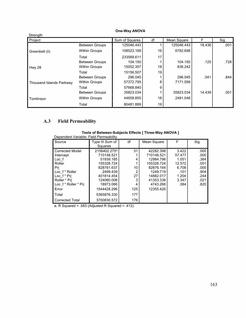
163
One-Way ANOVA
Strength
Project Sum of Squares df Mean Square F Sig.
Greenbelt (ii)
Between Groups 125046.443 1 125046.443 18.436 .001
Within Groups 108523.169 16 6782.698
Total 233569.611 17
Hwy 28
Between Groups 104.150 1 104.150 .125 .728
Within Groups 15052.357 18 836.242 Total 15156.507 19
Thousand Islands Parkway
Between Groups 296.045 1 296.045 .041 .844
Within Groups 57372.795 8 7171.599 Total 57668.840 9
Tomlinson
Between Groups 35823.034 1 35823.034 14.439 .001
Within Groups 44658.855 18 2481.048
Total 80481.889 19
A.3 Field Permeability
Tests of Between-Subjects Effects [ Three-Way ANOVA ]
Dependent Variable: Field Permeability
Source Type III Sum of Squares
df Mean Square F Sig.
Corrected Model 2156402.275a 51 42282.398 3.422 .000 Intercept 710148.521 1 710148.521 57.477 .000 Loc_f 51939.185 4 12984.796 1.051 .384 Roller 155328.724 1 155328.724 12.572 .001 Prj 828761.637 10 82876.164 6.708 .000 Loc_f * Roller 2499.439 2 1249.719 .101 .904 Loc_f * Prj 401814.454 27 14882.017 1.204 .244 Roller * Prj 124060.008 3 41353.336 3.347 .021 Loc_f * Roller * Prj 18973.066 4 4743.266 .384 .820
Error 1544428.296 125 12355.426 Total 5365876.330 177 Corrected Total 3700830.572 176 a. R Squared = .583 (Adjusted R Squared = .412)
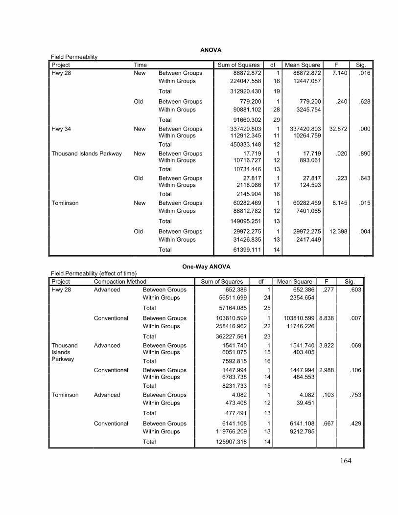
164
ANOVA
Field Permeability
Project Time Sum of Squares df Mean Square F Sig.
Hwy 28 New Between Groups 88872.872 1 88872.872 7.140 .016
Within Groups 224047.558 18 12447.087 Total 312920.430 19
Old Between Groups 779.200 1 779.200 .240 .628
Within Groups 90881.102 28 3245.754 Total 91660.302 29
Hwy 34 New Between Groups 337420.803 1 337420.803 32.872 .000 Within Groups 112912.345 11 10264.759 Total 450333.148 12
Thousand Islands Parkway New Between Groups 17.719 1 17.719 .020 .890 Within Groups 10716.727 12 893.061 Total 10734.446 13
Old Between Groups 27.817 1 27.817 .223 .643 Within Groups 2118.086 17 124.593 Total 2145.904 18
Tomlinson New Between Groups 60282.469 1 60282.469 8.145 .015
Within Groups 88812.782 12 7401.065 Total 149095.251 13
Old Between Groups 29972.275 1 29972.275 12.398 .004
Within Groups 31426.835 13 2417.449 Total 61399.111 14
One-Way ANOVA
Field Permeability (effect of time)
Project Compaction Method Sum of Squares df Mean Square F Sig.
Hwy 28 Advanced Between Groups 652.386 1 652.386 .277 .603
Within Groups 56511.699 24 2354.654 Total 57164.085 25
Conventional Between Groups 103810.599 1 103810.599 8.838 .007
Within Groups 258416.962 22 11746.226 Total 362227.561 23
Thousand Islands Parkway
Advanced Between Groups 1541.740 1 1541.740 3.822 .069 Within Groups 6051.075 15 403.405 Total 7592.815 16
Conventional Between Groups 1447.994 1 1447.994 2.988 .106 Within Groups 6783.738 14 484.553 Total 8231.733 15
Tomlinson Advanced Between Groups 4.082 1 4.082 .103 .753
Within Groups 473.408 12 39.451 Total 477.491 13
Conventional Between Groups 6141.108 1 6141.108 .667 .429
Within Groups 119766.209 13 9212.785 Total 125907.318 14
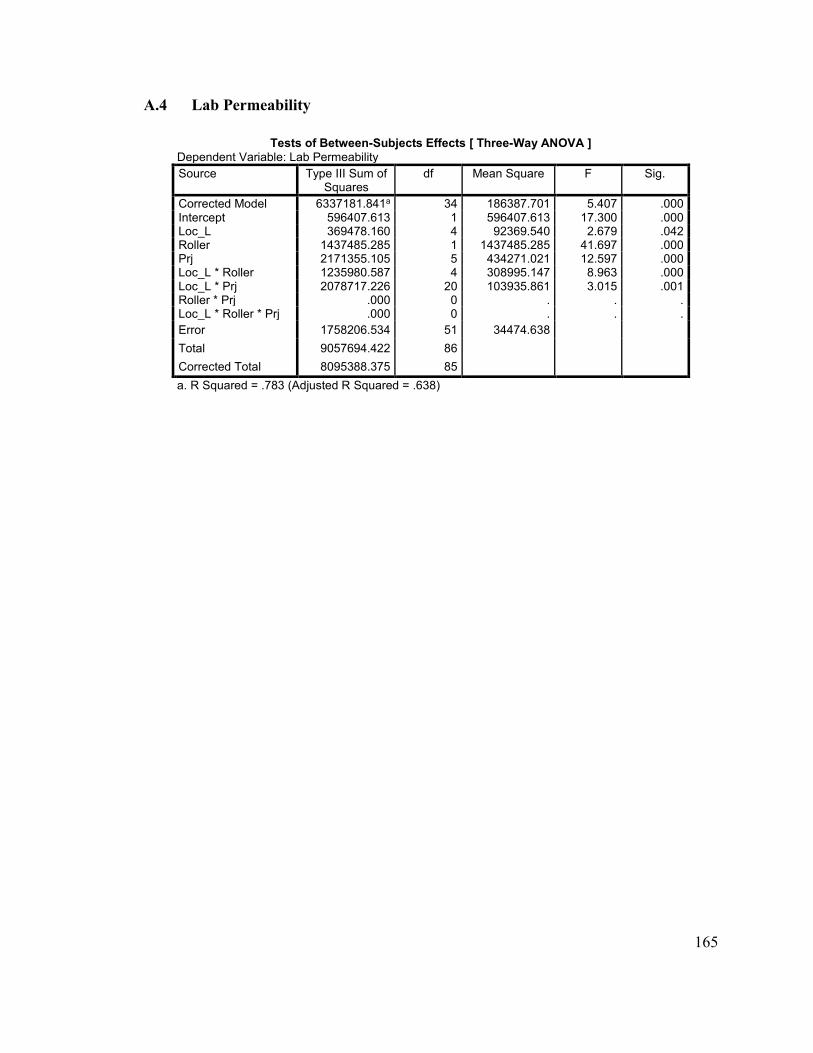
165
A.4 Lab Permeability
Tests of Between-Subjects Effects [ Three-Way ANOVA ]
Dependent Variable: Lab Permeability
Source Type III Sum of Squares
df Mean Square F Sig.
Corrected Model 6337181.841a 34 186387.701 5.407 .000 Intercept 596407.613 1 596407.613 17.300 .000 Loc_L 369478.160 4 92369.540 2.679 .042 Roller 1437485.285 1 1437485.285 41.697 .000 Prj 2171355.105 5 434271.021 12.597 .000 Loc_L * Roller 1235980.587 4 308995.147 8.963 .000 Loc_L * Prj 2078717.226 20 103935.861 3.015 .001 Roller * Prj .000 0 . . . Loc_L * Roller * Prj .000 0 . . .
Error 1758206.534 51 34474.638 Total 9057694.422 86 Corrected Total 8095388.375 85 a. R Squared = .783 (Adjusted R Squared = .638)

166
A.5 Lab vs. Field Permeability
Independent Samples Test
All Sites Levene's Test for Equality of Variances
t-test for Equality of Means
F Sig. t df Sig. (2-tailed) Mean Difference
Std. Error Difference
95% Confidence Interval of the Difference
Lower Upper
Equal variances assumed 19.766 .000 5.781 105 .000 71.31651 12.33626 46.85599 95.77703
Equal variances not assumed 5.863 87.276 .000 71.31651 12.16279 47.14272 95.49030
Independent Samples Test
Highway 16 Levene's Test for Equality of Variances
t-test for Equality of Means
F Sig. t df Sig. (2-tailed) Mean Difference
Std. Error Difference
95% Confidence Interval of the Difference
Lower Upper
K Equal variances assumed 1.379 .251 2.692 27 .012 72.76738 27.02829 17.30991 128.22485
Equal variances not assumed 2.666 24.190 .013 72.76738 27.29251 16.46178 129.07298
Independent Samples Test
Highway 17 Levene's Test for Equality of Variances
t-test for Equality of Means
F Sig. t df Sig. (2-tailed) Mean Difference
Std. Error Difference
95% Confidence Interval of the Difference
Lower Upper
Equal variances assumed 5.457 .028 5.254 25 .000 95.02615 18.08803 57.77315 132.27915
Equal variances not assumed 5.329 22.927 .000 95.02615 17.83028 58.13491 131.91740
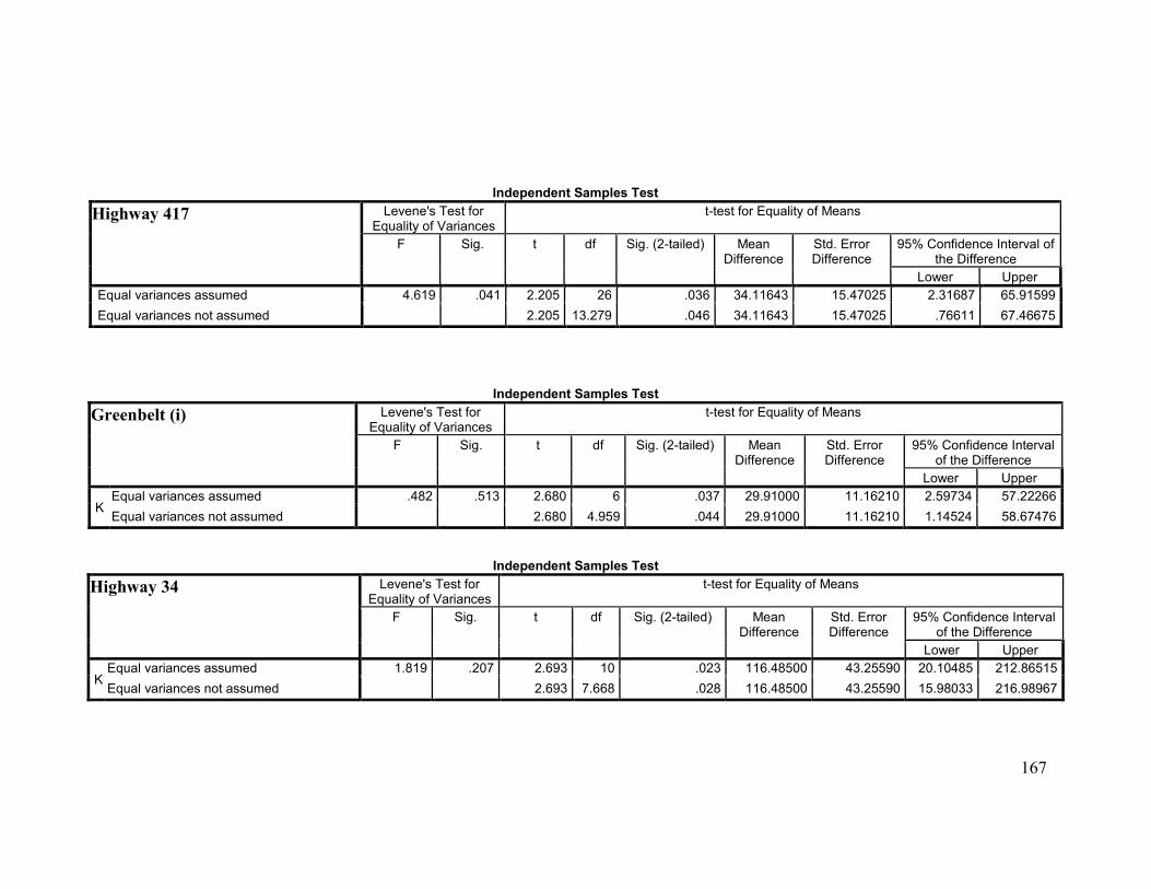
167
Independent Samples Test
Highway 417 Levene's Test for Equality of Variances
t-test for Equality of Means
F Sig. t df Sig. (2-tailed) Mean Difference
Std. Error Difference
95% Confidence Interval of the Difference
Lower Upper
Equal variances assumed 4.619 .041 2.205 26 .036 34.11643 15.47025 2.31687 65.91599
Equal variances not assumed 2.205 13.279 .046 34.11643 15.47025 .76611 67.46675
Independent Samples Test
Greenbelt (i) Levene's Test for Equality of Variances
t-test for Equality of Means
F Sig. t df Sig. (2-tailed) Mean Difference
Std. Error Difference
95% Confidence Interval of the Difference
Lower Upper
K Equal variances assumed .482 .513 2.680 6 .037 29.91000 11.16210 2.59734 57.22266
Equal variances not assumed 2.680 4.959 .044 29.91000 11.16210 1.14524 58.67476
Independent Samples Test
Highway 34 Levene's Test for Equality of Variances
t-test for Equality of Means
F Sig. t df Sig. (2-tailed) Mean Difference
Std. Error Difference
95% Confidence Interval of the Difference
Lower Upper
K Equal variances assumed 1.819 .207 2.693 10 .023 116.48500 43.25590 20.10485 212.86515
Equal variances not assumed 2.693 7.668 .028 116.48500 43.25590 15.98033 216.98967
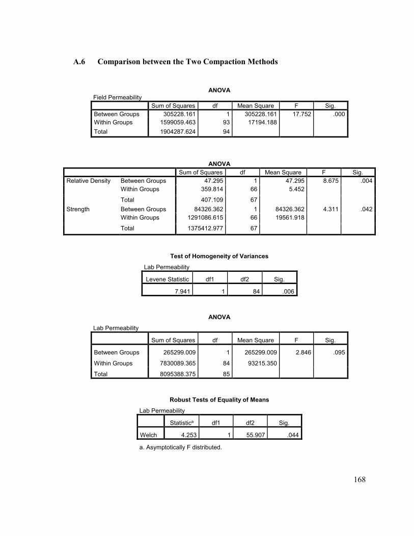
168
A.6 Comparison between the Two Compaction Methods
ANOVA
Field Permeability
Sum of Squares df Mean Square F Sig.
Between Groups 305228.161 1 305228.161 17.752 .000
Within Groups 1599059.463 93 17194.188 Total 1904287.624 94
ANOVA
Sum of Squares df Mean Square F Sig.
Relative Density Between Groups 47.295 1 47.295 8.675 .004
Within Groups 359.814 66 5.452 Total 407.109 67
Strength Between Groups 84326.362 1 84326.362 4.311 .042
Within Groups 1291086.615 66 19561.918 Total 1375412.977 67
Test of Homogeneity of Variances
Lab Permeability
Levene Statistic df1 df2 Sig.
7.941 1 84 .006
ANOVA
Lab Permeability
Sum of Squares df Mean Square F Sig.
Between Groups 265299.009 1 265299.009 2.846 .095
Within Groups 7830089.365 84 93215.350
Total 8095388.375 85
Robust Tests of Equality of Means
Lab Permeability
Statistica df1 df2 Sig.
Welch 4.253 1 55.907 .044
a. Asymptotically F distributed.
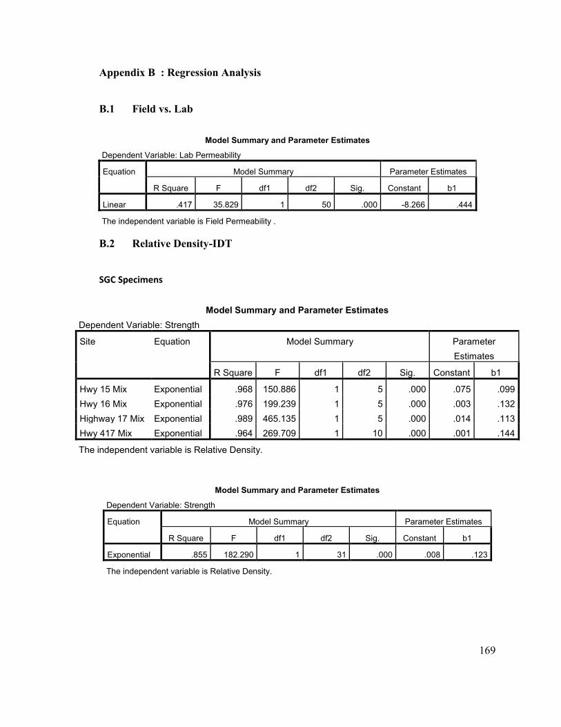
169
Appendix B : Regression Analysis
B.1 Field vs. Lab
Model Summary and Parameter Estimates
Dependent Variable: Lab Permeability
Equation Model Summary Parameter Estimates
R Square F df1 df2 Sig. Constant b1
Linear .417 35.829 1 50 .000 -8.266 .444
The independent variable is Field Permeability .
B.2 Relative Density-IDT
SGC Specimens
Model Summary and Parameter Estimates
Dependent Variable: Strength
Site Equation Model Summary Parameter
Estimates
R Square F df1 df2 Sig. Constant b1
Hwy 15 Mix Exponential .968 150.886 1 5 .000 .075 .099
Hwy 16 Mix Exponential .976 199.239 1 5 .000 .003 .132
Highway 17 Mix Exponential .989 465.135 1 5 .000 .014 .113
Hwy 417 Mix Exponential .964 269.709 1 10 .000 .001 .144
The independent variable is Relative Density.
Model Summary and Parameter Estimates
Dependent Variable: Strength
Equation Model Summary Parameter Estimates
R Square F df1 df2 Sig. Constant b1
Exponential .855 182.290 1 31 .000 .008 .123
The independent variable is Relative Density.
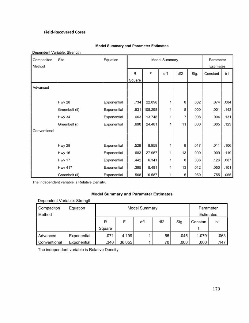
170
Field-Recovered Cores
Model Summary and Parameter Estimates
Dependent Variable: Strength
Compaciton
Method
Site Equation Model Summary Parameter
Estimates
R
Square
F df1 df2 Sig. Constant b1
Advanced
Hwy 28 Exponential .734 22.096 1 8 .002 .074 .084
Greenbelt (ii) Exponential .931 108.298 1 8 .000 .001 .143
Hwy 34 Exponential .663 13.748 1 7 .008 .004 .131
Greenbelt (i) Exponential .690 24.481 1 11 .000 .005 .123
Conventional
Hwy 28 Exponential .528 8.959 1 8 .017 .011 .106
Hwy 16 Exponential .683 27.957 1 13 .000 .009 .119
Hwy 17 Exponential .442 6.341 1 8 .036 .126 .087
Hwy 417 Exponential .395 8.481 1 13 .012 .050 .101
Greenbelt (ii) Exponential .568 6.587 1 5 .050 .755 .065
The independent variable is Relative Density.
Model Summary and Parameter Estimates
Dependent Variable: Strength
Compaciton
Method
Equation Model Summary Parameter
Estimates
R
Square
F df1 df2 Sig. Constan
t
b1
Advanced Exponential .071 4.199 1 55 .045 1.079 .063
Conventional Exponential .340 36.055 1 70 .000 .000 .147
The independent variable is Relative Density.
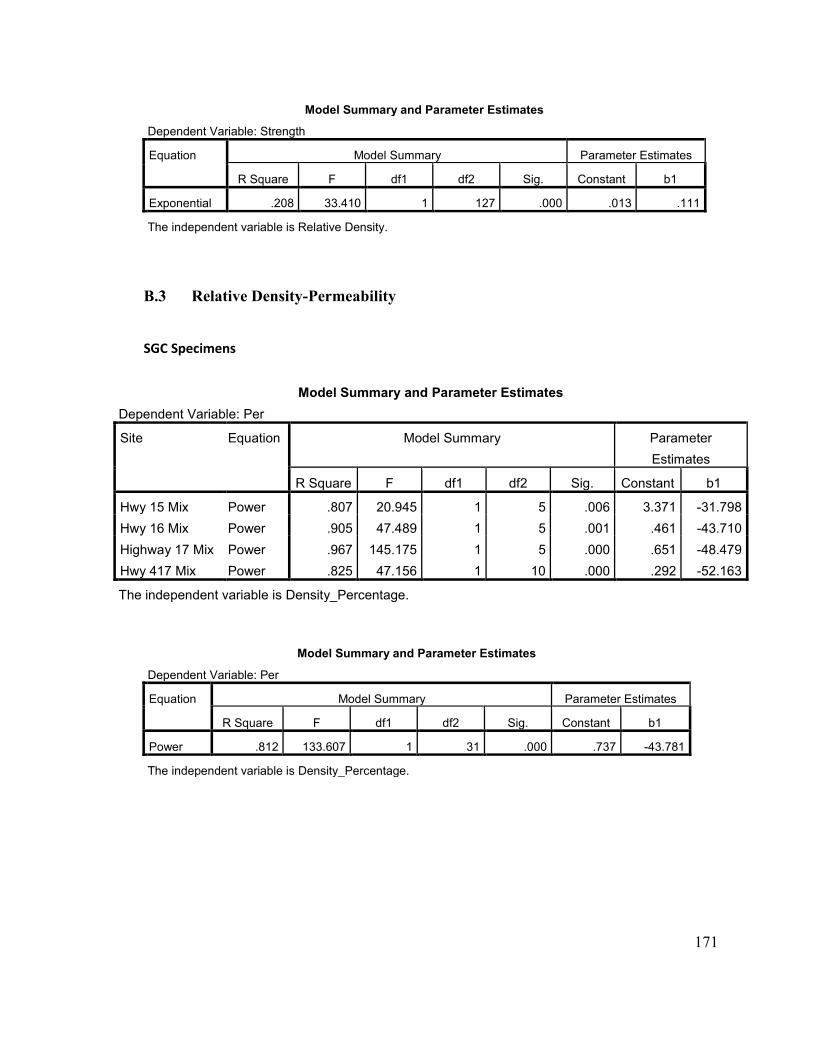
171
Model Summary and Parameter Estimates
Dependent Variable: Strength
Equation Model Summary Parameter Estimates
R Square F df1 df2 Sig. Constant b1
Exponential .208 33.410 1 127 .000 .013 .111
The independent variable is Relative Density.
B.3 Relative Density-Permeability
SGC Specimens
Model Summary and Parameter Estimates
Dependent Variable: Per
Site Equation Model Summary Parameter
Estimates
R Square F df1 df2 Sig. Constant b1
Hwy 15 Mix Power .807 20.945 1 5 .006 3.371 -31.798
Hwy 16 Mix Power .905 47.489 1 5 .001 .461 -43.710
Highway 17 Mix Power .967 145.175 1 5 .000 .651 -48.479
Hwy 417 Mix Power .825 47.156 1 10 .000 .292 -52.163
The independent variable is Density_Percentage.
Model Summary and Parameter Estimates
Dependent Variable: Per
Equation Model Summary Parameter Estimates
R Square F df1 df2 Sig. Constant b1
Power .812 133.607 1 31 .000 .737 -43.781
The independent variable is Density_Percentage.
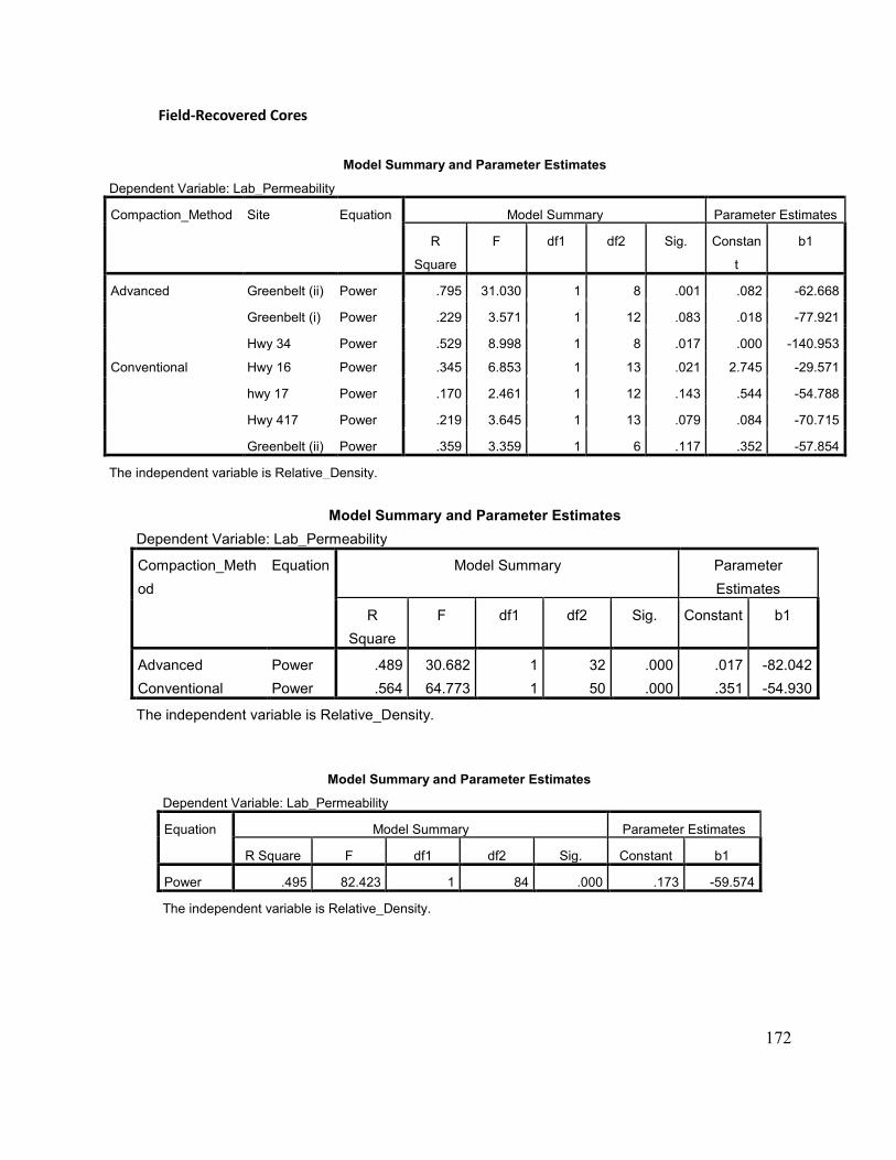
172
Field-Recovered Cores
Model Summary and Parameter Estimates
Dependent Variable: Lab_Permeability
Compaction_Method Site Equation Model Summary Parameter Estimates
R
Square
F df1 df2 Sig. Constan
t
b1
Advanced Greenbelt (ii) Power .795 31.030 1 8 .001 .082 -62.668
Greenbelt (i) Power .229 3.571 1 12 .083 .018 -77.921
Hwy 34 Power .529 8.998 1 8 .017 .000 -140.953
Conventional Hwy 16 Power .345 6.853 1 13 .021 2.745 -29.571
hwy 17 Power .170 2.461 1 12 .143 .544 -54.788
Hwy 417 Power .219 3.645 1 13 .079 .084 -70.715
Greenbelt (ii) Power .359 3.359 1 6 .117 .352 -57.854
The independent variable is Relative_Density.
Model Summary and Parameter Estimates
Dependent Variable: Lab_Permeability
Compaction_Meth
od
Equation Model Summary Parameter
Estimates
R
Square
F df1 df2 Sig. Constant b1
Advanced Power .489 30.682 1 32 .000 .017 -82.042
Conventional Power .564 64.773 1 50 .000 .351 -54.930
The independent variable is Relative_Density.
Model Summary and Parameter Estimates
Dependent Variable: Lab_Permeability
Equation Model Summary Parameter Estimates
R Square F df1 df2 Sig. Constant b1
Power .495 82.423 1 84 .000 .173 -59.574
The independent variable is Relative_Density.
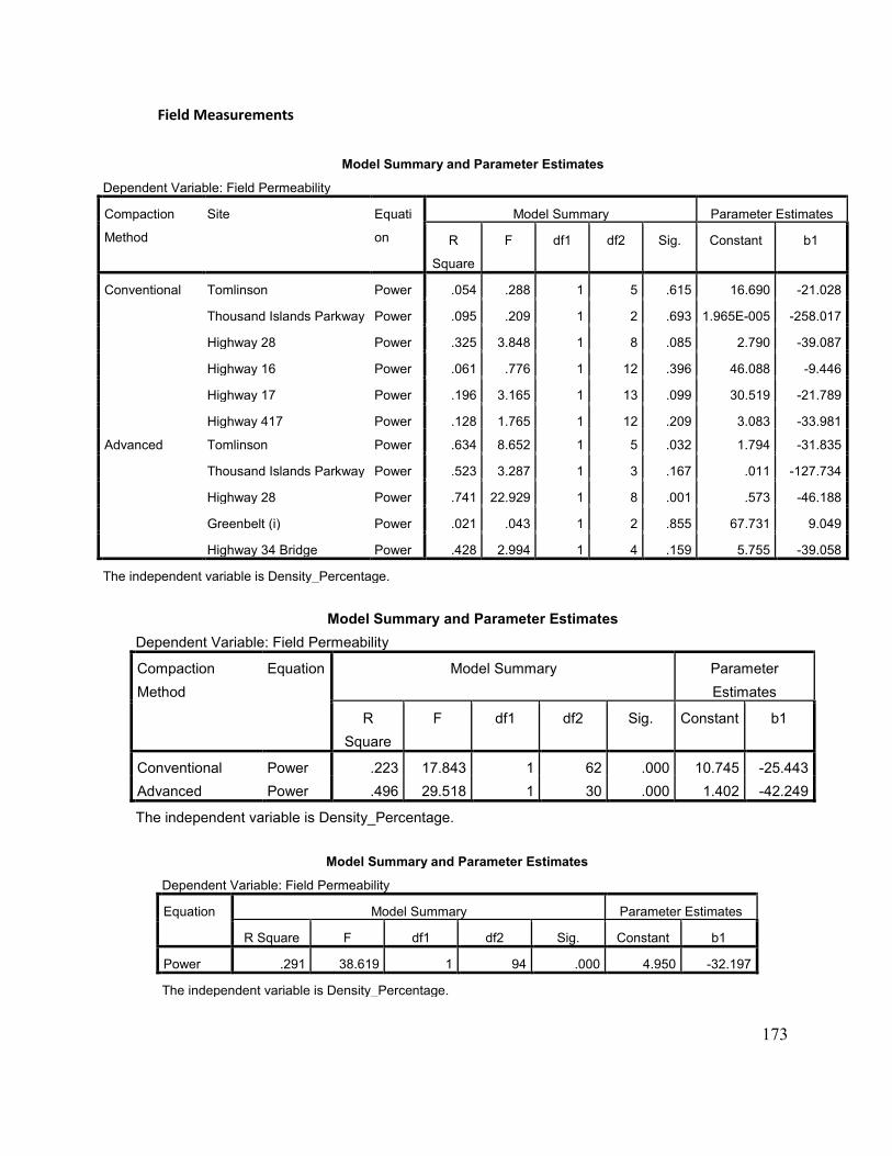
173
Field Measurements
Model Summary and Parameter Estimates
Dependent Variable: Field Permeability
Compaction
Method
Site Equati
on
Model Summary Parameter Estimates
R
Square
F df1 df2 Sig. Constant b1
Conventional Tomlinson Power .054 .288 1 5 .615 16.690 -21.028
Thousand Islands Parkway Power .095 .209 1 2 .693 1.965E-005 -258.017
Highway 28 Power .325 3.848 1 8 .085 2.790 -39.087
Highway 16 Power .061 .776 1 12 .396 46.088 -9.446
Highway 17 Power .196 3.165 1 13 .099 30.519 -21.789
Highway 417 Power .128 1.765 1 12 .209 3.083 -33.981
Advanced Tomlinson Power .634 8.652 1 5 .032 1.794 -31.835
Thousand Islands Parkway Power .523 3.287 1 3 .167 .011 -127.734
Highway 28 Power .741 22.929 1 8 .001 .573 -46.188
Greenbelt (i) Power .021 .043 1 2 .855 67.731 9.049
Highway 34 Bridge Power .428 2.994 1 4 .159 5.755 -39.058
The independent variable is Density_Percentage.
Model Summary and Parameter Estimates
Dependent Variable: Field Permeability
Compaction
Method
Equation Model Summary Parameter
Estimates
R
Square
F df1 df2 Sig. Constant b1
Conventional Power .223 17.843 1 62 .000 10.745 -25.443
Advanced Power .496 29.518 1 30 .000 1.402 -42.249
The independent variable is Density_Percentage.
Model Summary and Parameter Estimates
Dependent Variable: Field Permeability
Equation Model Summary Parameter Estimates
R Square F df1 df2 Sig. Constant b1
Power .291 38.619 1 94 .000 4.950 -32.197
The independent variable is Density_Percentage.
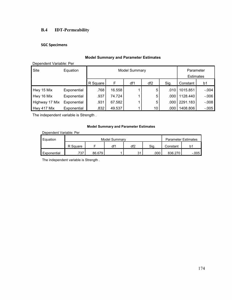
174
B.4 IDT-Permeability
SGC Specimens
Model Summary and Parameter Estimates
Dependent Variable: Per
Site Equation Model Summary Parameter
Estimates
R Square F df1 df2 Sig. Constant b1
Hwy 15 Mix Exponential .768 16.558 1 5 .010 1015.851 -.004
Hwy 16 Mix Exponential .937 74.724 1 5 .000 1128.440 -.006
Highway 17 Mix Exponential .931 67.582 1 5 .000 2291.183 -.008
Hwy 417 Mix Exponential .832 49.537 1 10 .000 1408.806 -.005
The independent variable is Strength .
Model Summary and Parameter Estimates
Dependent Variable: Per
Equation Model Summary Parameter Estimates
R Square F df1 df2 Sig. Constant b1
Exponential .737 86.679 1 31 .000 836.270 -.005
The independent variable is Strength .
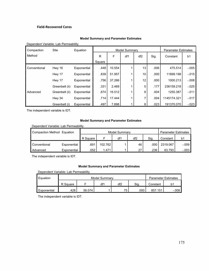
175
Field-Recovered Cores
Model Summary and Parameter Estimates
Dependent Variable: Lab Permeability
Compaction
Method
Site Equation Model Summary Parameter Estimates
R
Square
F df1 df2 Sig. Constant b1
Conventional Hwy 16 Exponential .448 10.554 1 13 .006 475.514 -.005
Hwy 17 Exponential .839 51.957 1 10 .000 11899.198 -.015
Hwy 17 Exponential .756 37.266 1 12 .000 1000.213 -.008
Greenbelt (ii) Exponential .331 2.469 1 5 .177 236159.218 -.025
Advanced Greenbelt (ii) Exponential .674 16.512 1 8 .004 1255.387 -.011
Hwy 34 Exponential .714 17.444 1 7 .004 1145174.321 -.017
Greenbelt (i) Exponential .497 7.898 1 8 .023 191370.070 -.023
The independent variable is IDT.
Model Summary and Parameter Estimates
Dependent Variable: Lab Permeability
Compaction Method Equation Model Summary Parameter Estimates
R Square F df1 df2 Sig. Constant b1
Conventional Exponential .691 102.762 1 46 .000 2319.067 -.009
Advanced Exponential .052 1.471 1 27 .236 63.793 -.003
The independent variable is IDT.
Model Summary and Parameter Estimates
Dependent Variable: Lab Permeability
Equation Model Summary Parameter Estimates
R Square F df1 df2 Sig. Constant b1
Exponential .428 56.074 1 75 .000 857.151 -.008
The independent variable is IDT.
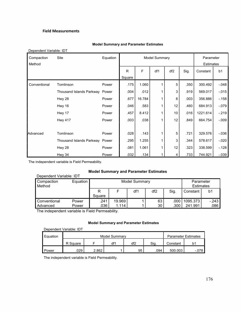
176
Field Measurements
Model Summary and Parameter Estimates
Dependent Variable: IDT
Compaction
Method
Site Equation Model Summary Parameter
Estimates
R
Square
F df1 df2 Sig. Constant b1
Conventional Tomlinson Power .175 1.060 1 5 .350 300.492 -.048
Thousand Islands Parkway Power .004 .012 1 3 .919 569.017 -.015
Hwy 28 Power .677 16.784 1 8 .003 356.886 -.158
Hwy 16 Power .046 .583 1 12 .460 684.913 -.079
Hwy 17 Power .457 8.412 1 10 .016 1221.614 -.219
Hwy 417 Power .003 .038 1 12 .849 664.754 -.009
Advanced Tomlinson Power .028 .143 1 5 .721 329.576 -.036
Thousand Islands Parkway Power .295 1.255 1 3 .344 578.617 -.020
Hwy 28 Power .081 1.061 1 12 .323 338.599 -.128
Hwy 34 Power .032 .134 1 4 .733 744.921 -.039
The independent variable is Field Permeability.
Model Summary and Parameter Estimates
Dependent Variable: IDT
Compaction Method
Equation Model Summary Parameter Estimates
R Square
F df1 df2 Sig. Constant b1
Conventional Power .241 19.969 1 63 .000 1095.373 -.243 Advanced Power .036 1.114 1 30 .300 241.991 .086
The independent variable is Field Permeability.
Model Summary and Parameter Estimates
Dependent Variable: IDT
Equation Model Summary Parameter Estimates
R Square F df1 df2 Sig. Constant b1
Power .029 2.862 1 95 .094 500.003 -.078
The independent variable is Field Permeability.

177