Field Demonstration and Validation of a New Device for ... · Field Demonstration and Validation of a New Device for ... SOP Standard operating procedure ... OF THE METER KD IS GREATER

Environmental Security Technology Certification Program

(ESTCP)

Final Report

Field Demonstration and Validation of a New Device for Measuring Water and Solute Fluxes at CFB Borden

November 2006

University of Florida

Distribution Statement A: Approved for Public Release, Distribution is Unlimited

Table of Contents

LIST OF ACRONYMS ..............................................................................................................III

LIST OF FIGURES ..................................................................................................................... V

LIST OF TABLES .................................................................................................................... VII

EXECUTIVE SUMMARY ......................................................................................................... X

1.0. INTRODUCTION.................................................................................................................. 1 1.1. BACKGROUND....................................................................................................................... 1 1.2. OBJECTIVES OF THE DEMONSTRATION .................................................................................. 1 1.3. DOD DIRECTIVES.................................................................................................................. 2 1.4. STAKEHOLDER/END-USER ISSUES ........................................................................................ 2

2.0. TECHNOLOGY DESCRIPTION........................................................................................ 3 2.1. TECHNOLOGY DEVELOPMENT AND APPLICATION ................................................................. 3 2.2. PREVIOUS TESTING OF THE TECHNOLOGY........................................................................... 18 2.3. FACTORS AFFECTING COST AND PERFORMANCE ................................................................ 18 2.4. ADVANTAGES AND LIMITATIONS OF THE TECHNOLOGY ..................................................... 18

3.0. DEMONSTRATION DESIGN........................................................................................... 19 3.1. PERFORMANCE OBJECTIVES................................................................................................ 19 3.2. SELECTING TEST SITE ......................................................................................................... 20 3.3. TEST SITE HISTORY/CHARACTERISTICS .............................................................................. 20 3.4. PRESENT OPERATIONS ........................................................................................................ 21 3.5. PRE-DEMONSTRATION TESTING AND ANALYSIS ................................................................. 21 3.6. TESTING AND EVALUATION PLAN ....................................................................................... 21 3.7. SELECTION OF ANALYTICAL/TESTING METHODS................................................................ 26 3.8. SELECTION OF ANALYTICAL/TESTING LABORATORY.......................................................... 26 3.9. MANAGEMENT AND STAFFING ............................................................................................ 26 3.10. DEMONSTRATION SCHEDULE ............................................................................................ 26

4.0. PERFORMANCE ASSESSMENT..................................................................................... 27

4.1. PERFORMANCE CRITERIA.................................................................................................... 27 4.2 PERFORMANCE CONFIRMATION METHODS .......................................................................... 27 4.3. DATA ANALYSIS, INTERPRETATION AND EVALUATION....................................................... 30

5.0. COST ASSESSMENT ......................................................................................................... 63

5.1 COST REPORTING ................................................................................................................. 63 5.2. COST ANALYSIS .................................................................................................................. 63 5.3 COST COMPARISON .............................................................................................................. 67

i

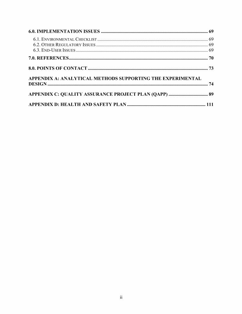
6.0. IMPLEMENTATION ISSUES .......................................................................................... 69 6.1. ENVIRONMENTAL CHECKLIST ............................................................................................. 69 6.2. OTHER REGULATORY ISSUES .............................................................................................. 69 6.3. END-USER ISSUES ............................................................................................................... 69

7.0. REFERENCES..................................................................................................................... 70

8.0. POINTS OF CONTACT ..................................................................................................... 73

APPENDIX A: ANALYTICAL METHODS SUPPORTING THE EXPERIMENTAL DESIGN ....................................................................................................................................... 74

APPENDIX C: QUALITY ASSURANCE PROJECT PLAN (QAPP) ................................. 89

APPENDIX D: HEALTH AND SAFETY PLAN .................................................................. 111

ii

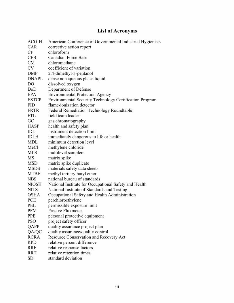
List of Acronyms

ACGIH American Conference of Governmental Industrial Hygienists CAR corrective action report CF chloroform CFB Canadian Force Base CM chloromethane CV coefficient of variation DMP 2,4-dimethyl-3-pentanol DNAPL dense nonaqueous phase liquid DO dissolved oxygen DoD Department of Defense EPA Environmental Protection Agency ESTCP Environmental Security Technology Certification Program FID flame-ionization detector FRTR Federal Remediation Technology Roundtable FTL field team leader GC gas chromatography HASP health and safety plan IDL instrument detection limit IDLH immediately dangerous to life or health MDL minimum detection level MeCl methylene chloride MLS multilevel samplers MS matrix spike MSD matrix spike duplicate MSDS materials safety data sheets MTBE methyl tertiary butyl ether NBS national bureau of standards NIOSH National Institute for Occupational Safety and Health NITS National Institute of Standards and Testing OSHA Occupational Safety and Health Administration PCE perchloroethylene PEL permissible exposure limit PFM Passive Fluxmeter PPE personal protective equipment PSO project safety officer QAPP quality assurance project plan QA/QC quality assurance/quality control RCRA Resource Conservation and Recovery Act RPD relative percent difference RRF relative response factors RRT relative retention times SD standard deviation

iii

SOP Standard operating procedure SRM Standard Reference Materials SSO site safety officer TCE trichloroethylene TLV threshold limit value TWA time weighted averages VOA volatile organic acid

iv

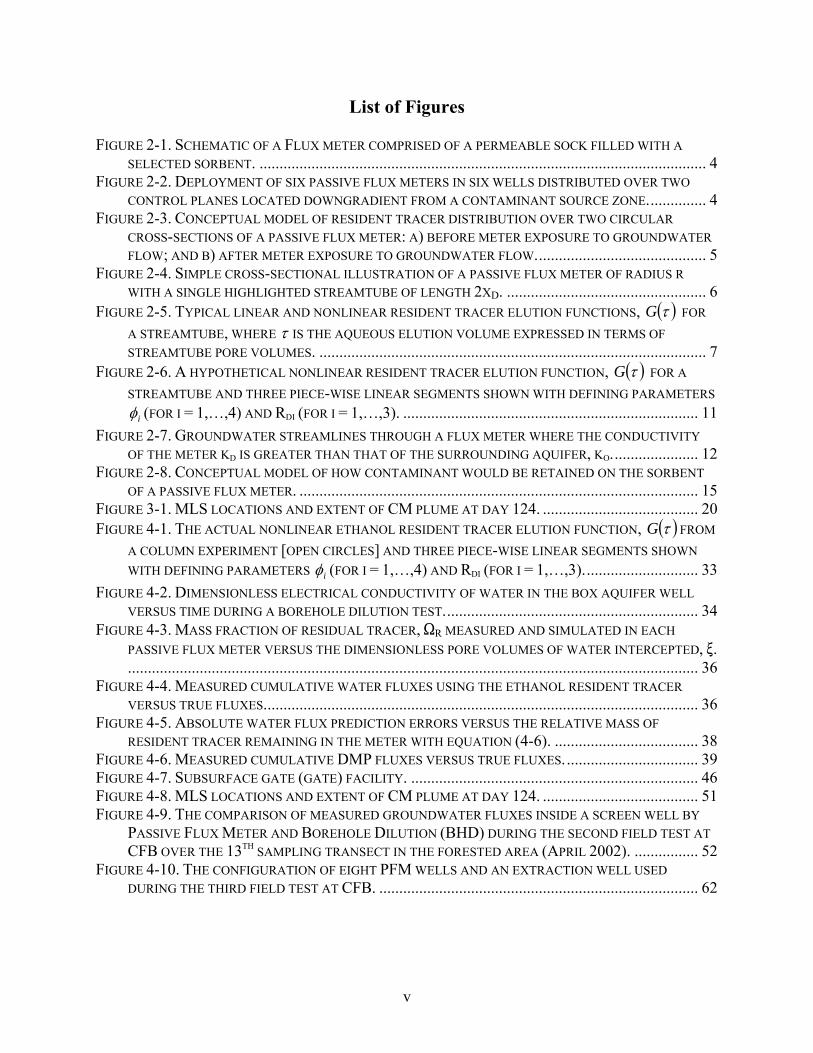
List of Figures FIGURE 2-1. SCHEMATIC OF A FLUX METER COMPRISED OF A PERMEABLE SOCK FILLED WITH A

SELECTED SORBENT. ................................................................................................................ 4 FIGURE 2-2. DEPLOYMENT OF SIX PASSIVE FLUX METERS IN SIX WELLS DISTRIBUTED OVER TWO

CONTROL PLANES LOCATED DOWNGRADIENT FROM A CONTAMINANT SOURCE ZONE............... 4 FIGURE 2-3. CONCEPTUAL MODEL OF RESIDENT TRACER DISTRIBUTION OVER TWO CIRCULAR

CROSS-SECTIONS OF A PASSIVE FLUX METER: A) BEFORE METER EXPOSURE TO GROUNDWATER FLOW; AND B) AFTER METER EXPOSURE TO GROUNDWATER FLOW........................................... 5

FIGURE 2-4. SIMPLE CROSS-SECTIONAL ILLUSTRATION OF A PASSIVE FLUX METER OF RADIUS R WITH A SINGLE HIGHLIGHTED STREAMTUBE OF LENGTH 2XD. .................................................. 6

FIGURE 2-5. TYPICAL LINEAR AND NONLINEAR RESIDENT TRACER ELUTION FUNCTIONS, ( )τG FOR

A STREAMTUBE, WHERE τ IS THE AQUEOUS ELUTION VOLUME EXPRESSED IN TERMS OF STREAMTUBE PORE VOLUMES. ................................................................................................. 7

FIGURE 2-6. A HYPOTHETICAL NONLINEAR RESIDENT TRACER ELUTION FUNCTION, ( )τG FOR A

STREAMTUBE AND THREE PIECE-WISE LINEAR SEGMENTS SHOWN WITH DEFINING PARAMETERS

iφ (FOR I = 1,…,4) AND RDI (FOR I = 1,…,3). .......................................................................... 11 FIGURE 2-7. GROUNDWATER STREAMLINES THROUGH A FLUX METER WHERE THE CONDUCTIVITY

OF THE METER KD IS GREATER THAN THAT OF THE SURROUNDING AQUIFER, KO...................... 12 FIGURE 2-8. CONCEPTUAL MODEL OF HOW CONTAMINANT WOULD BE RETAINED ON THE SORBENT

OF A PASSIVE FLUX METER. .................................................................................................... 15 FIGURE 3-1. MLS LOCATIONS AND EXTENT OF CM PLUME AT DAY 124. ....................................... 20 FIGURE 4-1. THE ACTUAL NONLINEAR ETHANOL RESIDENT TRACER ELUTION FUNCTION, ( )τG FROM

A COLUMN EXPERIMENT [OPEN CIRCLES] AND THREE PIECE-WISE LINEAR SEGMENTS SHOWN WITH DEFINING PARAMETERS iφ (FOR I = 1,…,4) AND RDI (FOR I = 1,…,3)............................. 33

FIGURE 4-2. DIMENSIONLESS ELECTRICAL CONDUCTIVITY OF WATER IN THE BOX AQUIFER WELL VERSUS TIME DURING A BOREHOLE DILUTION TEST................................................................ 34

FIGURE 4-3. MASS FRACTION OF RESIDUAL TRACER, SR MEASURED AND SIMULATED IN EACH PASSIVE FLUX METER VERSUS THE DIMENSIONLESS PORE VOLUMES OF WATER INTERCEPTED, >................................................................................................................................................ 36

FIGURE 4-4. MEASURED CUMULATIVE WATER FLUXES USING THE ETHANOL RESIDENT TRACER VERSUS TRUE FLUXES............................................................................................................. 36

FIGURE 4-5. ABSOLUTE WATER FLUX PREDICTION ERRORS VERSUS THE RELATIVE MASS OF RESIDENT TRACER REMAINING IN THE METER WITH EQUATION (4-6). .................................... 38

FIGURE 4-6. MEASURED CUMULATIVE DMP FLUXES VERSUS TRUE FLUXES.................................. 39 FIGURE 4-7. SUBSURFACE GATE (GATE) FACILITY. ........................................................................ 46 FIGURE 4-8. MLS LOCATIONS AND EXTENT OF CM PLUME AT DAY 124. ....................................... 51 FIGURE 4-9. THE COMPARISON OF MEASURED GROUNDWATER FLUXES INSIDE A SCREEN WELL BY

PASSIVE FLUX METER AND BOREHOLE DILUTION (BHD) DURING THE SECOND FIELD TEST AT CFB OVER THE 13TH SAMPLING TRANSECT IN THE FORESTED AREA (APRIL 2002). ................ 52

FIGURE 4-10. THE CONFIGURATION OF EIGHT PFM WELLS AND AN EXTRACTION WELL USED DURING THE THIRD FIELD TEST AT CFB. ................................................................................ 62

v

FIGURE 5-1. COST OF MEASURING WATER AND CONTAMINANT FLUXES BY PFMS AND THE BHD/MLS METHOD AS A FUNCTION OF THE NUMBER OF WELLS MONITORED........................ 68

vi

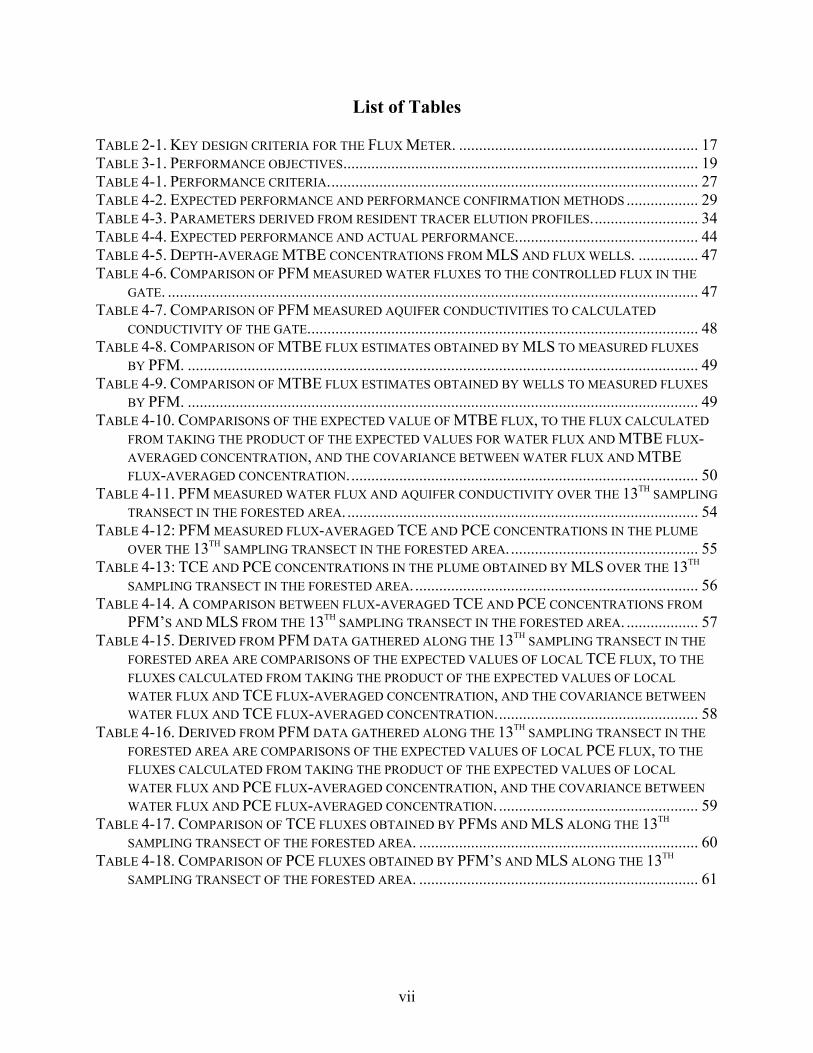
List of Tables TABLE 2-1. KEY DESIGN CRITERIA FOR THE FLUX METER. ............................................................ 17 TABLE 3-1. PERFORMANCE OBJECTIVES......................................................................................... 19 TABLE 4-1. PERFORMANCE CRITERIA............................................................................................. 27 TABLE 4-2. EXPECTED PERFORMANCE AND PERFORMANCE CONFIRMATION METHODS .................. 29 TABLE 4-3. PARAMETERS DERIVED FROM RESIDENT TRACER ELUTION PROFILES........................... 34 TABLE 4-4. EXPECTED PERFORMANCE AND ACTUAL PERFORMANCE.............................................. 44 TABLE 4-5. DEPTH-AVERAGE MTBE CONCENTRATIONS FROM MLS AND FLUX WELLS. ............... 47 TABLE 4-6. COMPARISON OF PFM MEASURED WATER FLUXES TO THE CONTROLLED FLUX IN THE

GATE. ..................................................................................................................................... 47 TABLE 4-7. COMPARISON OF PFM MEASURED AQUIFER CONDUCTIVITIES TO CALCULATED

CONDUCTIVITY OF THE GATE.................................................................................................. 48 TABLE 4-8. COMPARISON OF MTBE FLUX ESTIMATES OBTAINED BY MLS TO MEASURED FLUXES

BY PFM. ................................................................................................................................ 49 TABLE 4-9. COMPARISON OF MTBE FLUX ESTIMATES OBTAINED BY WELLS TO MEASURED FLUXES

BY PFM. ................................................................................................................................ 49 TABLE 4-10. COMPARISONS OF THE EXPECTED VALUE OF MTBE FLUX, TO THE FLUX CALCULATED

FROM TAKING THE PRODUCT OF THE EXPECTED VALUES FOR WATER FLUX AND MTBE FLUX-AVERAGED CONCENTRATION, AND THE COVARIANCE BETWEEN WATER FLUX AND MTBE FLUX-AVERAGED CONCENTRATION........................................................................................ 50

TABLE 4-11. PFM MEASURED WATER FLUX AND AQUIFER CONDUCTIVITY OVER THE 13TH SAMPLING TRANSECT IN THE FORESTED AREA......................................................................................... 54

TABLE 4-12: PFM MEASURED FLUX-AVERAGED TCE AND PCE CONCENTRATIONS IN THE PLUME OVER THE 13TH SAMPLING TRANSECT IN THE FORESTED AREA................................................ 55

TABLE 4-13: TCE AND PCE CONCENTRATIONS IN THE PLUME OBTAINED BY MLS OVER THE 13 SAMPLING TRANSECT IN THE FORESTED AREA.

TH

....................................................................... 56TABLE 4-14. A COMPARISON BETWEEN FLUX-AVERAGED TCE AND PCE CONCENTRATIONS FROM

PFM’S AND MLS FROM THE 13TH SAMPLING TRANSECT IN THE FORESTED AREA. .................. 57 TABLE 4-15. DERIVED FROM PFM DATA GATHERED ALONG THE 13TH SAMPLING TRANSECT IN THE

FORESTED AREA ARE COMPARISONS OF THE EXPECTED VALUES OF LOCAL TCE FLUX, TO THE FLUXES CALCULATED FROM TAKING THE PRODUCT OF THE EXPECTED VALUES OF LOCAL WATER FLUX AND TCE FLUX-AVERAGED CONCENTRATION, AND THE COVARIANCE BETWEEN WATER FLUX AND TCE FLUX-AVERAGED CONCENTRATION................................................... 58

TABLE 4-16. DERIVED FROM PFM DATA GATHERED ALONG THE 13TH SAMPLING TRANSECT IN THE FORESTED AREA ARE COMPARISONS OF THE EXPECTED VALUES OF LOCAL PCE FLUX, TO THE FLUXES CALCULATED FROM TAKING THE PRODUCT OF THE EXPECTED VALUES OF LOCAL WATER FLUX AND PCE FLUX-AVERAGED CONCENTRATION, AND THE COVARIANCE BETWEEN WATER FLUX AND PCE FLUX-AVERAGED CONCENTRATION. .................................................. 59

TABLE 4-17. COMPARISON OF TCE FLUXES OBTAINED BY PFMS AND MLS ALONG THE 13TH SAMPLING TRANSECT OF THE FORESTED AREA. ...................................................................... 60

TABLE 4-18. COMPARISON OF PCE FLUXES OBTAINED BY PFM’S AND MLS ALONG THE 13TH SAMPLING TRANSECT OF THE FORESTED AREA. ...................................................................... 61

vii

TABLE 4-19. COMPARISONS OF MEASURED WATER FLUX AND CONTAMINANT MASS FLOWS AT AN EXTRACTION WELL TO SPATIALLY INTEGRATED PFM MEASUREMENTS. ................................ 62

TABLE 5-1. COST TRACKING FOR PFM DEPLOYMENT. THE COSTS CONSIDERED HERE ARE FOR SITE CHARACTERIZATION ASSUMING 10 WELLS ARE SAMPLED WITH 10 FEET OF SCREEN IN EACH WELL...................................................................................................................................... 64

TABLE 5-2. COST TRACKING FOR BHD/MLS DEPLOYMENT. THE COSTS CONSIDERED HERE ARE FOR SITE CHARACTERIZATION ASSUMING 10 MLS WITH ONE FOOT VERTICAL SAMPLING INTERVAL............................................................................................................................... 66

viii

ACKNOWLEDGEMENTS We would like to express our gratitude to Drs John Cherry and Elizabeth Parker of University of Waterloo for the field support provided at the Canadian Forces Base Borden.

ix

Executive Summary The use of contaminant flux and contaminant mass discharge as robust metrics for assessment of risks at contaminated sites, and for evaluating the performance of site remediation efforts has gained increasing acceptance within the scientific, regulatory and user communities. Such gradual increase in acceptance and use of innovative technologies is slower in the environmental community, requiring a sound theoretical basis accepted widely in the technical circles and field-scale demonstration at diverse sites. In 2001 ESTCP funded a project (CU-0114) to demonstrate and validate a new monitoring technology known as the passive flux meter (PFM). This device provides direct in situ measurements of both subsurface water and contaminant fluxes. The focus of this project was to demonstrate and validate the PFM for measuring simultaneously the groundwater and contaminant fluxes in contaminated aquifers. This report presents results of PFM demonstration/validation from a series of controlled field experiments conducted at the CFB Borden Demonstration Site in Ontario, Canada. The specific project objectives were to: 1) demonstrate and validate the flux meter as an innovative technology for direct in situ

measurement of cumulative water and contaminant fluxes in groundwater, 2) demonstrate and validate a methodology for interpreting source strength from point-wise

measurements of cumulative contaminant and water fluxes, and, 3) gather field data in support of an effort to transition of the technology from the innovative

testing phase to a point where it will receive regulatory and end user acceptance and stimulate commercialization

The scope of the demonstration/validation effort at CFB included working with the University of Waterloo to conduct two field tests where perchloroethylene (PCE) and trichloroethylene (TCE) were the primary groundwater contaminants and a third test where MTBE was the contaminant of interest. The location of the demonstration was the forested research site at CFB located 150 km north of Toronto, Ontario. Site geology was composed of a surficial sand layer that is approximately 3.5 m thick which overlies a clayey aquitard. The first of the three demonstration/validation tests used an on-site test gate for subsurface flow in which groundwater flow could be controlled, MTBE concentrations could be monitored using multilevel samplers (MLS), and both water and MTBE fluxes could be measured using PFM’s installed in wells of different construction. The test gate was 25-m long and 2 m wide and opened on one end. The saturated thickness of the aquifer in the gate was about 1.77 m (this includes 35 cm of capillary fringe). Steady flow was established from four pumping wells located in the closed end. The purpose of the first test was used to assess the efficacy of the PFM for measuring a known ground water flow rate. Two types of well construction were tested: fully screened 2 inch wells and fully screened 2 inch wells with a sand pack. In addition, because groundwater in the gate contained MTBE from a previous study, concentrations measured by MLS provided an

x

opportunity to calculate MTBE mass fluxes under known flow conditions. These calculated fluxes were then compared to measured MTBE fluxes from PFMs. Finally, the PFM water flux measurements under a known flow and hydraulic gradient provided a unique opportunity to test the PFM as a tool for measuring aquifer permeability. The second demonstration/validation field test took place in a controlled release plume where University of Waterloo released a DNAPL mixture consisting of 45% PCE, 45% TCE, and 10% Chloroform by weight. This mixture was released in April 9, 1999 from a single release point located 1.8 m below ground surface and 0.9 m below the water table. In the area of release, the aquifer was approximately 3 m thick consisting of fine to medium grained sand. The DNAPL release generated a dissolved plume approximately 80 m long that at one time was discharging into a small stream. University of Waterloo deployed a dense network of multilevel samplers to characterize this plume. The multi-level samplers (MLS) network consisted of approximately 20 transects of up to 20 MLS wells. Each transect completely span the width of the plume at various longitudinal distances from the point of DNAPL release. For the second test, PFM’s were used to measure water, TCE, and PCE fluxes in a fence-row wells located 1 meter down gradient from the13th MLS transect. Local TCE and PCE flux-averaged concentrations were obtained by taking the ratio of PFM measured water and contaminant fluxes. These calculated flux-averaged concentrations were then compared to TCE and PCE resident concentrations measured over the 13th MLS transect. Constituent concentrations gathered from MLS are generally assumed to represent flux-averaged concentrations wherever they are used in flux calculations. The second field test provides an opportunity to validate this assumption by comparing MLS concentrations to flux-averaged concentrations measured by PFM’s. Following the aforementioned analysis of water quality data, PFM measurements of water flux were compared to measured and calculated fluxes obtained from other widely accepted methods. Initially a comparison was made of water flux measures acquired by PFM and those obtained by borehole dilution. Because both methods provide direct measures flow through screened wells, results generated should be similar. Water fluxes measured by PFM were also compared to specific discharge estimates calculated using measured hydraulic gradients and aquifer conductivities obtained by independent sources. Finally, a simple comparison was made of aquifer conductivities measured by PFM’s to those gathered by other methods. The third and final test involved in situ measurements of water and contaminant fluxes within the capture zone of an interception well designed to capture the above described PCE/TCE plume. In this test, a ring of eight 1.25-inch fully screened monitoring wells were installed at a radial distance of 35 cm from a single extraction well. PFM’s installed in the wells enabled direct measures of both groundwater flow and TCE/PCE contaminant fluxes. The spatially integrated measures of specific discharge and PCE and TCE mass fluxes were compared to well-head measures of PCE and TCE mass flows and the discharge rate of the extraction well.

xi

Because this report constitutes the first of four reports on demonstration/validation studies performed at four different sites, this report also presents much underlying flux meter theory in Chapter 2, and in Chapter 4 results of several lab-scale studies that validate this theory. These results have since been published in peer-reviewed journals (Hatfield et al. 2004). Results from some of the Borden field demonstration have also been published (Annable et al 2005). With regards to the field demonstration/validation, it was expected that that the PFM would measure water fluxes within 15% of the induced flow rate in the gate. Actual performance was considerably better. Maximum absolute differences between the measured fluxes at any given well and the induced flux in the gate (8.23±0.66 cm/d) were less than -11.2 %. The maximum coefficient of variation for measured water fluxes was 0.6 in wells constructed with a filter pack and less than 1.3 for simple screened wells. The integrated water fluxes obtained from averaging results of three PFM installed in the same type of well were even closer to the induced flow rate: -2.3 % for screened wells and 0.7 percent for wells constructed with filter packs. Recently acquired evidence showed that the PFM can be used to measure aquifer conductivity. Measured aquifer conductivities were within 2% of the integrated values determined for the gate system (5.23 m/d) using the measured hydraulic gradient (0.016±0.002), the induce flow rate (203 ±3 ml/min), and the measured cross-sectional area of flow (3.55± 0.28 m2). To evaluate the PFM as a device for measuring contaminant fluxes, it was proposed that PFM measured MTBE fluxes would be compared to fluxes calculated from the induced specific discharge (8.23 cm/d) in the gate and an average MTBE concentration generated from measurements taken from wells and MLS in the gate. It was expected PFMs would measure contaminant fluxes within 25% of calculated fluxes from MLS data and well concentrations. The actual performance of the PFM is shown in Tables 4-8 and 4-9. Total MTBE fluxes, obtained from spatially integrating PFM measurements from FA wells (those without sand packs) compared within 16.63% of integrated calculations from MLS’s. For the FB wells containing sand packs, total MTBE fluxes were within 1.18 % of integrated calculations using depth-average MTBE concentrations from six flux wells and three MLS wells determined. For individual wells, the smallest absolute difference between PFM measured and calculated fluxes was 4.06% for a sand-packed well; while the largest was 93.16 % for a simple screened well. The coefficient of variation (CV) for PFM measured MTBE fluxes ranged from 0.31 to 2.53 depending again on whether a sand pack was used in well construction. The PFM measures water flux directly and the contaminant mass intercepted and retained on the device can be used to calculate local flux-averaged contaminant concentrations. It is shown for the gate experiments water flux and MTBE concentrations are strongly correlated; consequently, the expected flux cannot be approximated as simply the product of the mean water flux and the mean flux-averaged concentration derived from PFM measurements. For the field test involving the PCE/TCE plume, a successful comparison was assumed if groundwater and contaminant fluxes were estimated within 20 and 35% respectively. In this test water flux measurement obtained by PFM are compared to same generated by borehole dilution.

xii

Results indicate that the average absolute relative difference in measurements is 9.4%. These results are well within the performance criterion of less than 20% difference specified in the demonstration plan. Groundwater flux in the Forested area was reported to ranges between 5 to 8 cm/d. The average flux measured over the 13th transect was 6.62 cm/d with an estimated coefficient of variation of 0.33. The PFM estimated aquifer conductivities were comparable to estimates generated from the gate facility which is located immediately adjacent to the forested area. A higher level of uncertainty associated with contaminant flux measurements was expected in the demonstration plan to due to the nature of the MLS based estimates. Field data revealed that MLS contaminant concentrations were comparable to the flux-averaged TCE and PCE concentrations derived from PFM measurements in the plume. Coefficients of variation for MLS and PFM’s concentration data were both greater than 1.0 which would indicate significant variability. Averaged over the 13th sampling transect, differences between MLS and PFM concentrations data were 13.2% for TCE and 13% for PCE, which is well within the performance criterion of 35% indicated in the demonstration plan. However, concentration differences exceeding this criterion were recorded between individual wells. Results of PFM measurements of Water, TCE, and PCE fluxes along 13th sampling transect suggest water-flux-contaminant covariance is significant at certain wells. However, at the transect scale these covariances are 7 % of the total TCE flux and less than 12% for PCE. Hence, the expected flux can be approximated as the product of the mean water flux and the mean flux-averaged concentration. In addition this suggests that concentration data from MLS and an accurate estimate of the average water flux can be used to estimated the average contaminant flux at the transect scale. TCE and PCE fluxes calculated from MLS data were compared to PFM results. Clearly, large difference exist between individual PFM’s and MLS; however, much smaller differences exist between PFM and MLS estimates integrated over the transect (less than 25 % for TCE and 10% for PCE). For the third field test, acceptable comparisons with the flux meter results were taken to exist at 15 and 25% for groundwater and contaminant flux respectively. Water fluxes were estimated within 2% of the extraction flow rate, while TCE and PCE were respectively measured within 9 and 32% of the contaminant mass flow rate at the well head. Costs are calculated for the passive flux meter method (PFM) and the borehole dilution/ multilevel sample method (BHD/MLS) for contaminant flux characterization. Cost estimates indicate that the PFM method results in a lower unit cost per foot depending on cost variability; Site-specific conditions can lead to changes in the cost estimates for the alternate technology; however, a proper suite of resident tracers with a designed range in retardation factors and optimal deployment period permit a PFM to interrogate a wide range in groundwater fluxes at no additional costs. The principal cost drivers are mobilization/demobilization, labor, and sampling/analysis costs. Labor costs and analytical costs can easily vary by up to 50% and lead

xiii

to total unit costs (per linear foot) varying by about 20-33%. Costs for both the PFM and the BHD/MLS appear to be similar in terms of mobilization, materials, and analytical costs. The PFM generates cumulative measures of water and contaminant flux, while BHD/MLS method produces short-term evaluations that reflect current conditions and not long-term trends. Therefore, in the absence of continuous monitoring, it may be more cost effective and in the best interests of stakeholders to deploy systems designed to gather cumulative measures of water flow and contaminant mass flow. Cumulative monitoring devices like the PFM generate the same information derived from integrating continuous data. These systems should produce robust flux estimates that reflect long-term transport conditions and are less sensitive to day-to-day fluctuation in flow and contaminant concentration. Finally on a per-well basis, the time required to execute field operations are less for the PFM, than typically required to collect MLS samples or to conduct borehole dilutions on site.

xiv

1.0. Introduction

1.1. Background The Department of Defense (DoD) has a critical need for technologies that provided for cost-effective long-term monitoring of volatile organic chemicals, petroleum and related compounds, trace metals, and explosives. Active remediation systems such as “pump and treat”, passive remediation systems such as natural attenuation, and RCRA closure sites often require elaborate and expensive monitoring. This project demonstrates and validates the Passive Fluxmeter (PFM) which is a new technology that provides for direct in situ measurement of both cumulative subsurface water and contaminant fluxes. The flux meter is a technology that directly addresses the DoD need for cost-effective long-term monitoring, because flux measurements can be used for process control, for remedial action performance assessments, and for compliance purposes (Basu et al. 2006 and Newman et al. 2005 and 2006). The PFM is a self-contained permeable unit that is inserted into a well or boring such that it intercepts groundwater flow but does not retain it. The interior composition of the meter is a matrix of hydrophobic and hydrophilic permeable sorbents that retain dissolved organic and inorganic contaminants present in fluid intercepted by the unit. The sorbent matrix is also impregnated with known amounts of one or more fluid soluble ‘resident tracers’. These tracers are leached from the sorbent at rates proportional to the fluid flux. The meter is inserted into a well or boring and exposed to groundwater flow for a period ranging from days to months. Next, the meter is removed and the sorbent carefully extracted to quantify the mass of all contaminants intercepted and the residual masses of all resident tracers. The contaminants masses are used to calculate time-averaged contaminant mass fluxes, while residual resident tracer masses are used to calculate cumulative fluid flux. Existing, monitoring technologies cannot provide cumulative water and contaminant fluxes without continuous and therefore expensive sampling. 1.2. Objectives of the Demonstration The specific objectives of this demonstration project were to: 4) demonstrate and validate the flux meter as an innovative technology for direct in situ measurement of cumulative water and contaminant fluxes in groundwater, 5) demonstrate and validate a methodology for interpreting source strength from point-wise measurements of cumulative contaminant and water fluxes, and 3) gather field data in support of an effort to transition of the technology from the innovative testing phase to a point where it will receive regulatory and end user acceptance and stimulate commercialization. The location of the demonstration was the forested research site at Canadian Forces Base Borden located 150 km north of Toronto, Ontario. Site geology was composed of a surficial sand layer

1

that is approximately 3.5 m thick and overlies a clayey aquitard. Field tests with the flux meter were performed in the sandy surficial Borden aquifer where groundwater, perchloroethylene (PCE), trichloroethylene (TCE) and methyl tertiary butyl ether (MTBE) fluxes were measured. The scope of the demonstration project included working with the University of Waterloo to conduct three different field tests where PCE, TCE, and MTBE were the primary contaminants of interest. The first test used an on-site subsurface flow channel where groundwater flow could be controlled and MTBE fluxes could be calculated from monitored concentrations for comparison PFM measurements. The next field test involved a fence-row of flux meters deployed down gradient from a controlled release source zone where PFM measured groundwater, TCE and PCE fluxes. These fluxes were compared to independent estimates generated from taking the product of the estimated ambient groundwater flux and contaminant concentrations obtained by a fencerow of multilevel samplers located immediately up-gradient from the PFMs. For the third and final test, water and PCE and TCE fluxes were measured within the capture zone of a well designed to intercept an existing PCE/TCE plume. Spatial integration of the in situ PCE and TCE fluxes were compared to measured constituent masses flows at the extracted well. The two primary advantages of the PFM are first that it is the only instrument known to provide direct measurements of subsurface solute flux and second it provides simultaneous measures of both cumulative groundwater and contaminant fluxes. This demonstration project examines both of these advantages. Results obtained with the flux meter are compared to estimates obtained using the standard approach of calculating contaminant fluxes from monitored contaminant concentrations and measured or estimated groundwater fluxes. Standard methods typically require extensive aquifer characterization and costly water quality monitoring, and, as part of this project cost comparisons are performed. Finally, as part of this demonstration, statistics are developed and comparisons are drawn between solute and water fluxes derived from the PFM and flux estimates generated through alternative methods. 1.3. DoD Directives The Department of Defense (DoD) has a critical need for technologies that provided for cost-effective long-term monitoring of volatile organic chemicals, petroleum and related compounds, trace metals, and explosives. Active remediation systems such as “pump and treat” of groundwater and passive remediation systems such as natural attenuation as well as RCRA closure sites often require elaborate and expensive monitoring. This project demonstrates and validates PFM’s as a new technology for direct in situ measurement of both cumulative subsurface water and contaminant fluxes. Measurements of this nature can be used for process control and for both long- and short-term assessments of remedial action performance and compliance. 1.4. Stakeholder/End-User Issues There are three primary issues of concern to stakeholders/end-users: Issue 1: Will the flux meter yield correct results? Issue 2: Can the flux meter yield reliable results from long-term monitoring?

2

Issue 3: Are monitoring costs of the flux meter lower than the costs of traditional technologies? The demonstration addressed each issue of concern. With regards to the first issue, in situ flux measurements were compared to contaminant fluxes estimated from capture wells and from multilevel samplers. With regards to Issue 2, flux devices were installed for both short-term and long-term experiments. The duration of long-term experiments was be six weeks. Sorbents were selected to retain target contaminants and minimize the total depletion of tracers. Results of long-term monitoring were compared to contaminant fluxes derived from equivalent-term studies involving capture wells and multilevel samplers. The third and final issue was addressed through an analysis of costs incurred if traditional monitoring technologies were used to obtain comparable information on water and contaminant fluxes.

2.0. Technology Description

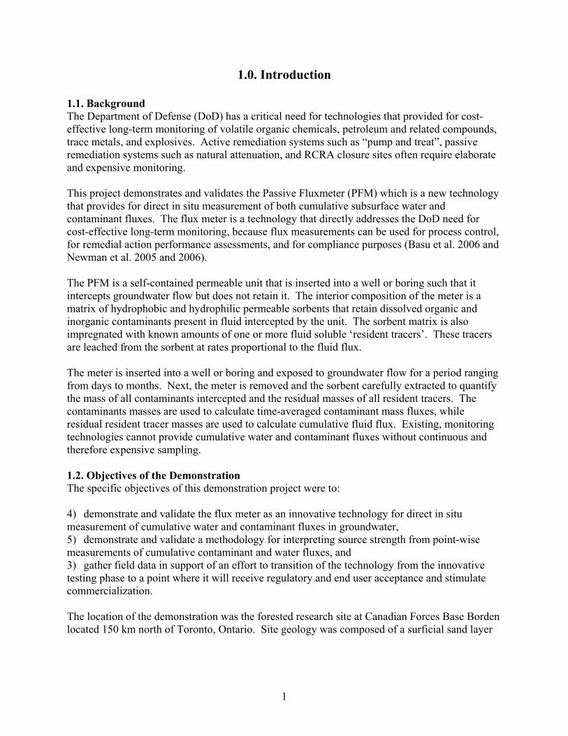
2.1. Technology Development and Application This demonstration report describes the proposed strategy for testing and validating the PFM technology for direct in situ measurement of both cumulative water and contaminant fluxes in groundwater. The PFM is a self-contained permeable unit that is inserted into a well or boring such that it intercepts groundwater flow but does not retain it (See Figure 1-1). The interior composition of the flux meter is a matrix of hydrophobic and hydrophilic permeable sorbents that retain dissolved organic and/or inorganic contaminants present in fluid intercepted by the unit. The sorbent matrix is also impregnated with known amounts of one or more fluid soluble ‘resident tracers’. These tracers are leached from the sorbent at rates proportional to fluid flux. After a specified period of exposure to groundwater flow, the flux meter is removed from the well or boring. Next, the sorbent is carefully extracted to quantify the mass of all contaminants intercepted by the flux meter and the residual masses of all resident tracers. The contaminants masses are used to calculate cumulative and time-averaged contaminant mass fluxes, while residual resident tracer masses are used to calculate cumulative or time- average fluid flux. Depth variations of both water and contaminant fluxes can be measured in an aquifer from a single flux meter by vertically segmenting the exposed sorbent packing, and analyzing for resident tracers and contaminants. Thus, at any specific well depth, an extraction from the locally exposed sorbent yields the mass of resident tracer remaining and the mass of contaminant intercepted. Note that multiple tracers with a range of partitioning coefficients are used to determine variability in groundwater flow with depth that could range over orders of magnitude. This data is used to estimate local cumulative water and contaminant fluxes.

3

The Flux Meter: A Permeable Sock Packed with Sorbent

Pipe Attached to Sock Used to Extract The Flux Meter from a Well

Rod Attached to End of Permeable Sock Used to Insert the Flux Meter into a Well

Figure 2-1. Schematic of a Flux meter comprised of a permeable sock filled with a selected sorbent.

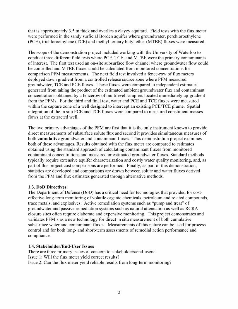
2.1.1. Theory (Measuring Water Flux) Figure 2-2 illustrates the deployment of six PFMs in six wells distributed over two transects located downgradient from a contaminant source but upgradient from a sentinel well. Depth variations of both water and contaminant fluxes can be measured in an aquifer from a single PFM by vertically segmenting the exposed sorbent packing; thus, at any specific well depth, an extraction from the locally exposed sorbent yields the mass of resident tracer remaining and the mass of contaminant intercepted.

Figure 2-2. Deployment of six passive flux meters in six wells distributed over two control planes located downgradient from a contaminant source zone.

4

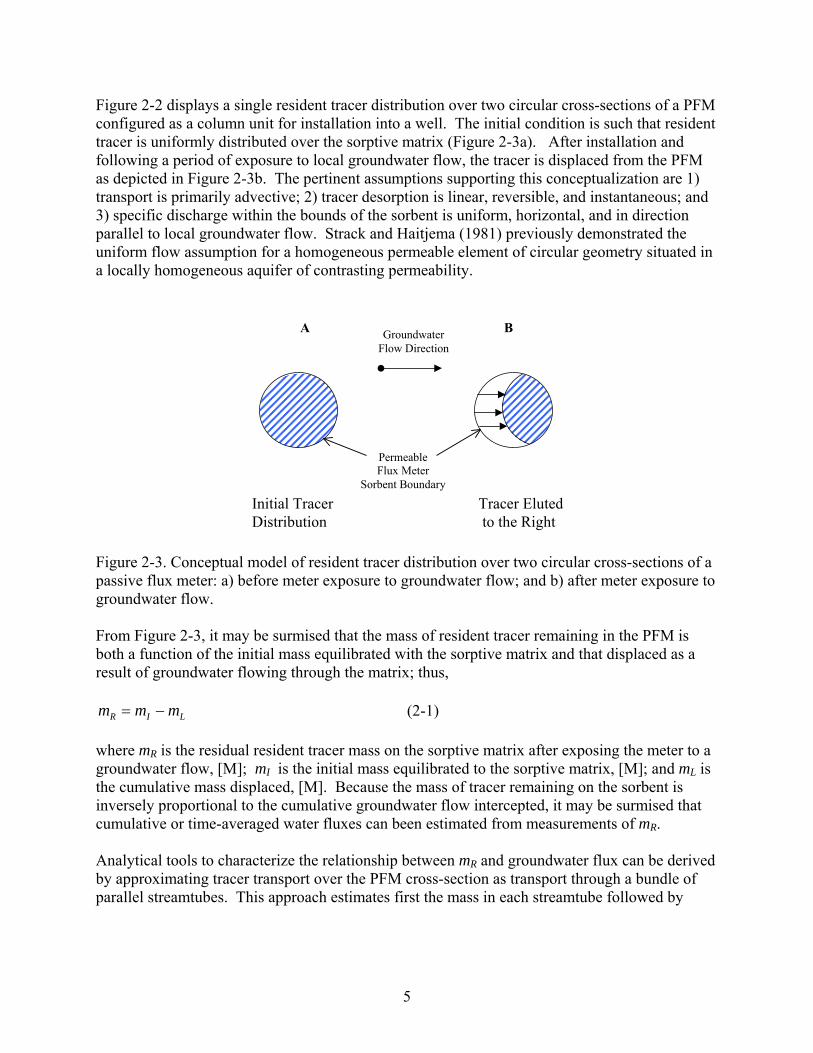
Figure 2-2 displays a single resident tracer distribution over two circular cross-sections of a PFM configured as a column unit for installation into a well. The initial condition is such that resident tracer is uniformly distributed over the sorptive matrix (Figure 2-3a). After installation and following a period of exposure to local groundwater flow, the tracer is displaced from the PFM as depicted in Figure 2-3b. The pertinent assumptions supporting this conceptualization are 1) transport is primarily advective; 2) tracer desorption is linear, reversible, and instantaneous; and 3) specific discharge within the bounds of the sorbent is uniform, horizontal, and in direction parallel to local groundwater flow. Strack and Haitjema (1981) previously demonstrated the uniform flow assumption for a homogeneous permeable element of circular geometry situated in a locally homogeneous aquifer of contrasting permeability.

B

Initial Tracer Distribution

Tracer Eluted to the Right

Groundwater Flow Direction

Permeable Flux Meter

Sorbent Boundary

A

Figure 2-3. Conceptual model of resident tracer distribution over two circular cross-sections of a passive flux meter: a) before meter exposure to groundwater flow; and b) after meter exposure to groundwater flow. From Figure 2-3, it may be surmised that the mass of resident tracer remaining in the PFM is both a function of the initial mass equilibrated with the sorptive matrix and that displaced as a result of groundwater flowing through the matrix; thus,

LIR mmm −= (2-1) where mR is the residual resident tracer mass on the sorptive matrix after exposing the meter to a groundwater flow, [M]; mI is the initial mass equilibrated to the sorptive matrix, [M]; and mL is the cumulative mass displaced, [M]. Because the mass of tracer remaining on the sorbent is inversely proportional to the cumulative groundwater flow intercepted, it may be surmised that cumulative or time-averaged water fluxes can been estimated from measurements of mR. Analytical tools to characterize the relationship between mR and groundwater flux can be derived by approximating tracer transport over the PFM cross-section as transport through a bundle of parallel streamtubes. This approach estimates first the mass in each streamtube followed by

5

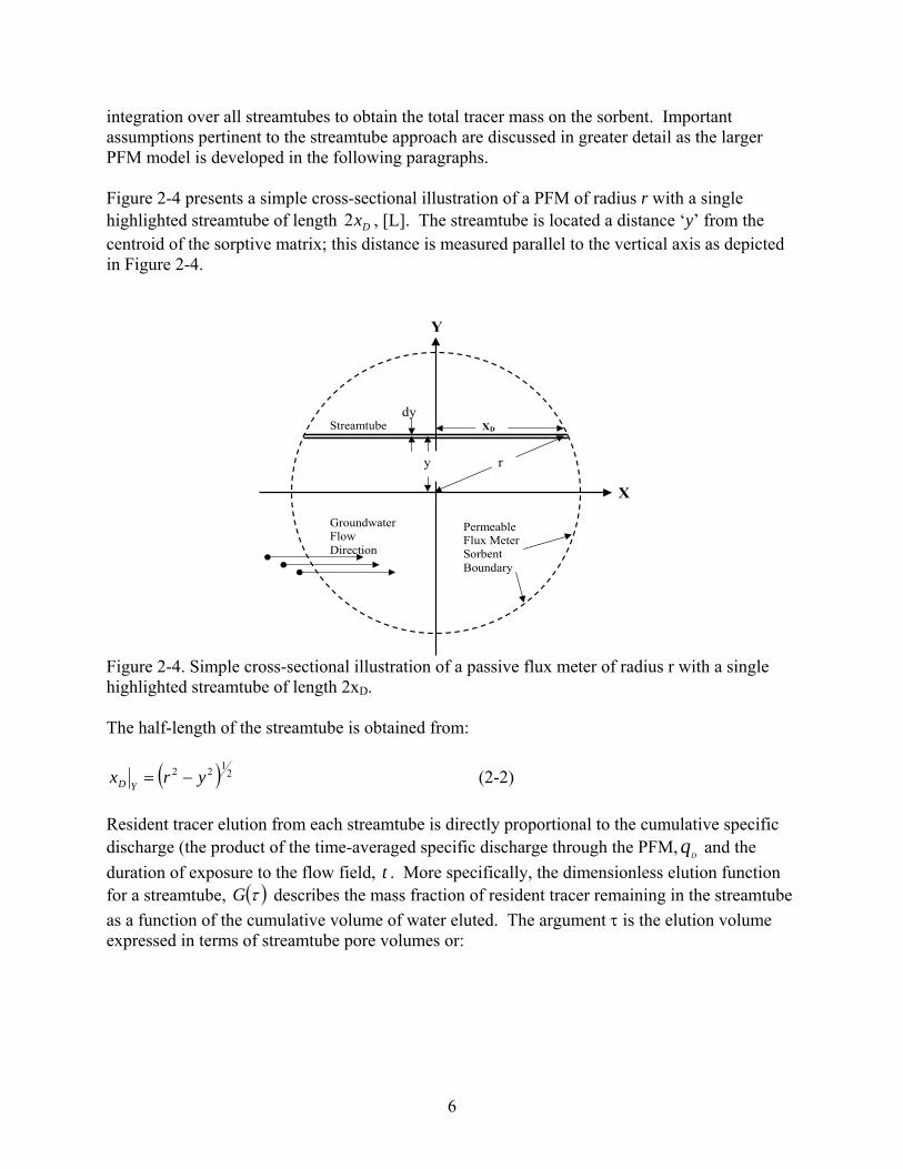
integration over all streamtubes to obtain the total tracer mass on the sorbent. Important assumptions pertinent to the streamtube approach are discussed in greater detail as the larger PFM model is developed in the following paragraphs. Figure 2-4 presents a simple cross-sectional illustration of a PFM of radius r with a single highlighted streamtube of length , [L]. The streamtube is located a distance ‘y’ from the centroid of the sorptive matrix; this distance is measured parallel to the vertical axis as depicted in Figure 2-4.

Dx2

Y

X

Permeable Flux Meter Sorbent Boundary

XD Streamtube

r y

dy

GroundwaterFlow Direction

Figure 2-4. Simple cross-sectional illustration of a passive flux meter of radius r with a single highlighted streamtube of length 2xD. The half-length of the streamtube is obtained from:

( ) 2122 yrx

YD −= (2-2) Resident tracer elution from each streamtube is directly proportional to the cumulative specific discharge (the product of the time-averaged specific discharge through the PFM, and the duration of exposure to the flow field, t . More specifically, the dimensionless elution function for a streamtube,

Dq

( )τG describes the mass fraction of resident tracer remaining in the streamtube as a function of the cumulative volume of water eluted. The argument τ is the elution volume expressed in terms of streamtube pore volumes or:

6

θτ

D

D

xtq

2= (2-3)

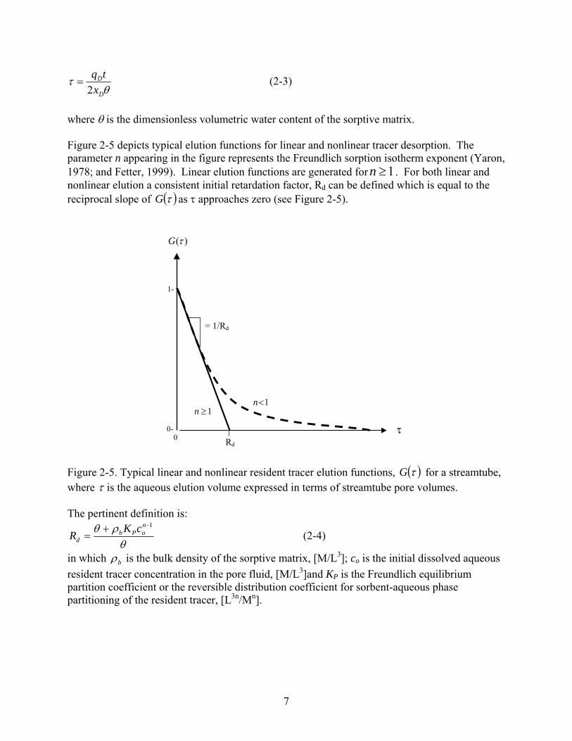
where θ is the dimensionless volumetric water content of the sorptive matrix. Figure 2-5 depicts typical elution functions for linear and nonlinear tracer desorption. The parameter n appearing in the figure represents the Freundlich sorption isotherm exponent (Yaron, 1978; and Fetter, 1999). Linear elution functions are generated for . For both linear and nonlinear elution a consistent initial retardation factor, R

1≥nd can be defined which is equal to the

reciprocal slope of ( )τG as τ approaches zero (see Figure 2-5).

0

1≥n

0-

1-

)(τG

1<n

τ

= 1/Rd

Rd Figure 2-5. Typical linear and nonlinear resident tracer elution functions, ( )τG for a streamtube, where τ is the aqueous elution volume expressed in terms of streamtube pore volumes. The pertinent definition is:

θρθ 1−+

=noPb

dcKR (2-4)

in which bρ is the bulk density of the sorptive matrix, [M/L3]; co is the initial dissolved aqueous resident tracer concentration in the pore fluid, [M/L3]and KP is the Freundlich equilibrium partition coefficient or the reversible distribution coefficient for sorbent-aqueous phase partitioning of the resident tracer, [L3n/Mn].

7

The product ( )τG and streamtube length quantify the mass fraction of tracer remaining in a streamtube; while the integration of this product over all streamtubes quantifies the mass fraction of resident tracer remaining in the PFM. This integration is made from the centroid of the sorptive matrix to a radial distance

Dx2

rr ≤max . Thus,

( )[ ]bdyxGbrm

mD

r

I

R

R22 max

0

2 ∫==Ω τπ

(2-5)

where represents the mass fraction of initial tracer remaining on the sorptive matrix after exposing the PFM to groundwater flow for period t; b is the thickness of the sorptive matrix or axial length of PFM column, [L]; and dy is the elemental width of the streamtube, [L]. The coefficient 2 appears outside the integral as it reflects the symmetry of integration taken over half the sorptive cross-section from y =0 to the upper limit . The value of is usually taken to equal

RΩ

maxr maxrr , the radius of the PFM when ( )τG is a continuous function for all values of 0≥τ .

Equation (2-5) serves to map residual resident tracer mass RΩ and cumulative specific discharge (or ) irrespective of desorption nonlinearities; it is only critical that tq

D Dq ( )τG be

continuous and known. Assuming ( )τG is linear (i.e., reflects linear elution because and desorption is instantaneous), an analytical formulation for

1≥n( )τG and equation (2-5) can be derived even

though the elution function is not continuous for all values of 0≥τ . This analytical expression is most convenient as it expresses explicitly time-averaged water flux ( or ) in terms of measured residual tracer mass m

Dq tq

D

R, parameters of PFM geometry (e.g., circular), and sorptive matrix properties (e.g., tracer partition coefficients). To develop this formulation, the streamtube concept is revisited with consideration given first to defining the initial tracer mass in the streamtube:

bdycRxdm odDI θ2= (2-6) where dmI is the initial elemental tracer mass contained in the streamtube, [M]. Because ( )τG is linear, the mass of tracer displaced from the streamtube is given by the following equation:

bdytcqdmODL

= (2-7) where dmL is the elemental tracer mass displaced, [M]. From equation (2-1), it is clear that equations (2-6) and (2-7) combine to obtain , the elemental mass of residual resident tracer in the streamtube, [M].

Rdm

8

bdytcqbdycRxdm oDodDR −= θ2 (2-8)

Finally, dividing equation (2-6) into (2-8) produces the following linear elution function ( )τG for a streamtube:

( )

⎪⎪⎩

⎪⎪⎨

⎧

>

≤−

==1

20

122

1

dD

D

dD

D

dD

D

I

R

Rxtqfor

Rxtqfor

Rxtq

dmdmG

θ

θθτ (2-9)

Because the linear elution function is discontinuous at ( ) 12 =

dDDRxtq θ and is zero for

( ) 12 >dDD

Rxtq θ , the upper integration limit, is chosen such that equation (2-9) may be substituted into equation (2-5). The concept of , as implemented herein, evolves from the realization that resident tracer is completely eluted from streamtubes less-than-or-equal to a length

maxr

maxr

χ :

d

DrI R

tqXθ

χ ==max

2 (2-10)

Thus, in equation (2-10) defines the transverse radial distance from the origin beyond which all resident tracer has been displaced from the cross section of the PFM. Hence,

maxr

for ; dmmaxry < R > 0 otherwise, for ; dmmaxry ≥ R = 0. Substituting equation (2-10) into (2-2) yields the pertinent definition of for linear elution: maxr

21

22

222

max 4 ⎟⎟⎠

⎞⎜⎜⎝

⎛−=

d

D

Rtqrr

θ (2-11)

Given relationships ( )τG and , equations (2-2), (2-5), (2-9) and (2-11) may be combined and the resulting expression integrated to yield the following dimensionless equation for the mass fraction of residual tracer on the PFM.

maxr

9

( )[ 221 11sin2 ξξξπ

−−−=Ω −

R] (2-12)

where

od

RR cRbr

mθπ 2=Ω (2-13)

and

d

D

Rrtq

θξ

2= (2-14)

The variable ξ represents the dimensionless cumulative pore volume of fluid intercepted by the device over the time period t divided by the retardation factor Rd. For the most part, an evaluation of equation (2-12) will show resident tracer being displaced at a rate linearly proportional to ξ ; as a result, it is feasible to use in lieu of (2-12), equation (2-15) below for values of 6.0≤ξ or : 32.0≥Ω

R

0.12.1 +−=Ω ξR (2-15)

Finally, from equations (2-14) and (2-15) a convenient formula is produced for estimating the time-averaged specific discharge, through the PFM. Dq

( )t

Rrq dRD

θΩ−=

167.1 (2-16)

Equations (2-12), (2-15), and (2-16) are strictly applicable to tracers producing linear elution functions ( ); however, for resident tracers producing concave elution functions (from

), the above developments are still useful if the nonlinear elution process can be described through a superposition of p independent linear elution functions. Under this approach, p linear elution functions

1≥n1<n

( )iG τ [i = 1,2,…p] are superimposed in τ to generate an approximate nonlinear

elution function comprised of p piecewise linear segments. Further analysis with ( )τG ( )τG produces a new equation for suitable for both linear and nonlinear tracer elution. RΩ

( ) ( )[ 221

11 11sin2

iii

p

iiiR ξξξφφ

π−−−−=Ω −

=+∑ ] (2-17)

and

10

di

Di Rr

tqθ

ξ2

= (2-18)

where index i (i = 1,2,…p), identifies each linear segment of the approximate elution function and each elution term of interest; the difference (φ i - φ i+1) quantifies the mass fraction of tracer eluted in accordance to function ( )iG τ under retardation factor Rd i, for (i = 1,2,…p). Equation (2-17) is simply a linear combination of terms, where each term possesses the same form as equation (2-12). The parameters of equation (2-17) can be extracted directly from a plot of , the piecewise linear approximation of the elution function

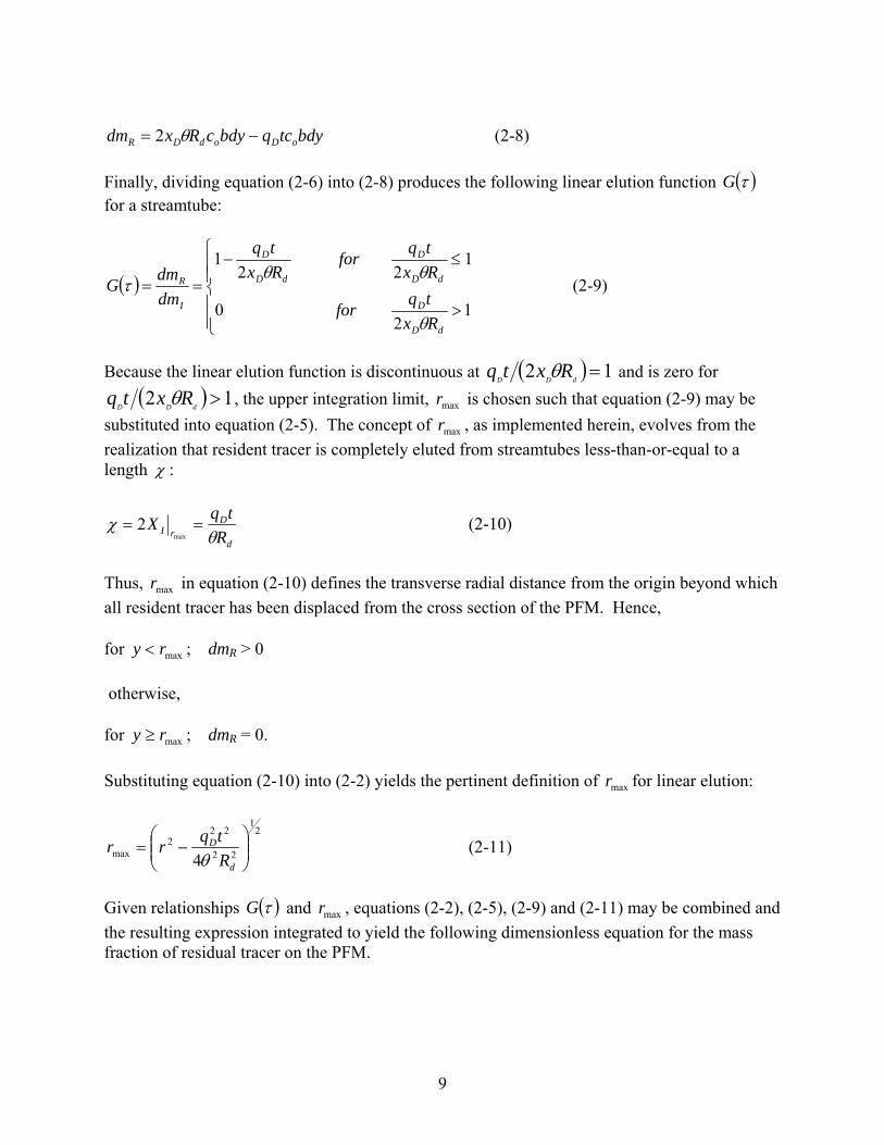
( )τG( )τG . In Figure 2-6, a hypothetical nonlinear elution

curve is illustrated along with an approximate function created with p=3 linear segments. The value of Rdi (for i = 1,2,and 3) is obtained from the terminating abscissa of segment i; whereas the value of φi , is the intercept of segment i extended to the vertical axis. Values of 1φ and

1+pφ are always 1 and 0 respectively; consequently, equation (2-17) reduces to the equation (2-14) for p =1.

3

2

1

2φ

0 4φ

1φ

0-

1-

)(τG

Rd1 Rd2 Rd3

3φ

τ

Figure 2-6. A hypothetical nonlinear resident tracer elution function, ( )τG for a streamtube and three piece-wise linear segments shown with defining parameters iφ (for i = 1,…,4) and Rdi (for i = 1,…,3). For purposes of obtaining convenient estimations of , applications of equations (2-15) and (2-16) can be extended to nonlinear eluting tracers. This is achieved by equating the value of R

Dq

d to

11

the reciprocal slope of ( )τG as 0→τ ; otherwise, the retardation factor appearing in (2-16) and (2-14) must be redefined as follows:

∑=

+−= p

i di

iid

R

R

1

1

1φφ

(2-19)

In the above discussion it is assumed here that can be measured with the PFM; although, the ultimate goal is to obtain the time-averaged specific discharge of the local groundwater, , [L/T]. Strack and Haitjema, (1981) and Klammler et al., (2006a) show that is linearly proportional to :

Dq

Oq

Dq

oq

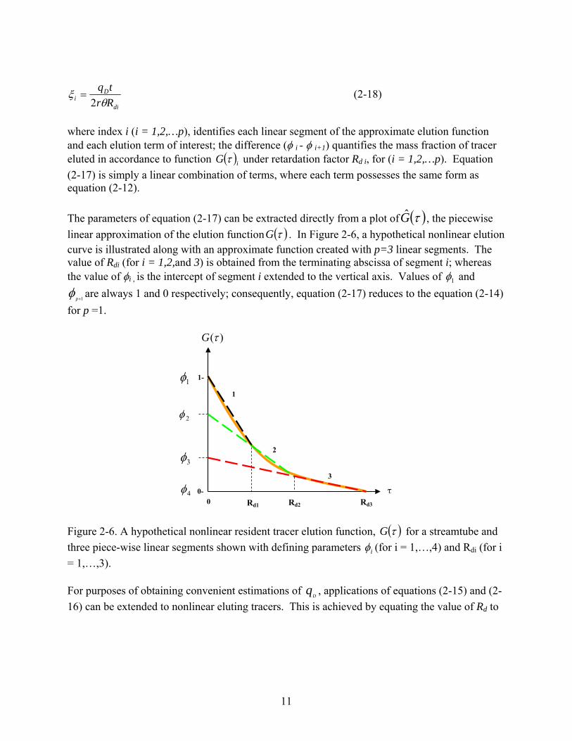
OD qq α= (2-20) where α characterizes the convergence or divergence of groundwater flow in the vicinity of the PFM. Figure 2-7 illustrates converging groundwater flow on the upgradient side of a meter, parallel streamlines or uniform flow inside the device, and diverging flow as water exits the meter; this depiction is consistent with the hydraulic conductivity of the sorptive matrix, being greater than that of the surrounding aquifer, and with a PFM installed in an open borehole (i.e., in the absence of a well screen).

Dk

Ok

kO

kd

Converging Streamlines

Permeable Flux Meter

Borehole Edge

Figure 2-7. Groundwater streamlines through a flux meter where the conductivity of the meter kd is greater than that of the surrounding aquifer, ko.

12

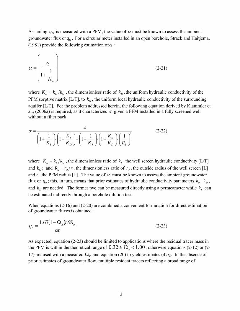
Assuming is measured with a PFM, the value of Dq α must be known to assess the ambient groundwater flux or .Oq For a circular meter installed in an open borehole, Strack and Haitjema, (1981) provide the following estimation ofα :

⎟⎟⎟⎟

⎠

⎞

⎜⎜⎜⎜

⎝

⎛

+=

DK11

2α (2-21)

where ODD kkK = , the dimensionless ratio of ,Dk the uniform hydraulic conductivity of the PFM sorptive matrix [L/T], to , the uniform local hydraulic conductivity of the surrounding aquifer [L/T]. For the problem addressed herein, the following equation derived by Klammler et al., (2006a) is required, as it characterizes

Ok

α given a PFM installed in a fully screened well without a filter pack.

21111111

4

⎟⎟⎠

⎞⎜⎜⎝

⎛⋅⎟⎟⎠

⎞⎜⎜⎝

⎛−⋅⎟⎟

⎠

⎞⎜⎜⎝

⎛−+⎟⎟

⎠

⎞⎜⎜⎝

⎛+⋅⎟⎟

⎠

⎞⎜⎜⎝

⎛+

=

SD

S

SD

S

S RKK

KKK

K

α (2-22)

where OSS kkK = , the dimensionless ratio of ,Sk the well screen hydraulic conductivity [L/T] and ; and Ok rrR OS = , the dimensionless ratio of , the outside radius of the well screen [L] and r , the PFM radius [L]. The value of

Orα must be known to assess the ambient groundwater

flux or ; this, in turn, means that prior estimates of hydraulic conductivity parameters , , and are needed. The former two can be measured directly using a permeameter while can be estimated indirectly through a borehole dilution test.

oq ok Dk

Sk Sk

When equations (2-16) and (2-20) are combined a convenient formulation for direct estimation of groundwater fluxes is obtained.

( )t

Rrq DR

O αθΩ−

=167.1

(2-23)

As expected, equation (2-23) should be limited to applications where the residual tracer mass in the PFM is within the theoretical range of 00.132.0 <Ω≤

R; otherwise equations (2-12) or (2-

17) are used with a measured and equation (20) to yield estimates of qRΩ O. In the absence of prior estimates of groundwater flow, multiple resident tracers reflecting a broad range of

13

retardation factors can be used to interpret a range of potential groundwater discharges. Taking this approach, one or more tracers are likely to remain in the PFM and within the preferable range of for the application of equation (2-23). RΩ The above analysis does not explicitly address competitive sorption/desorption, which can occur among multiple tracers co-eluted from a PFM. Competitive tracer interactions are generally embedded in all elution functions. More importantly, these interactions can produce elution profiles that vary with tracer combinations and initial concentrations. Assuming competitive resident tracer sorption/desorption occurs, the above analysis is applicable as long as the elution functions used are generated from co-elution experiments matching PFM conditions. For example, elution profiles are derived from experiments where tracers are eluted as a suite and with initial concentrations matching those used in PFMs. Finally, sorption nonequilibrium among tracers is not explicitly addressed in the above modeling. However, like competitive tracer sorption/desorption, rate-limited sorption is almost always present to some degree and as such is always embedded in measured elution profiles. Significant nonequilibrium tracer sorption produces an extended elution tail. Conditions giving rise to rate-limited sorption are widely discussed in the literature and are characterized in terms of dimensionless Damkohler numbers (Bahr and Rubin 1987). Assuming rate-limited sorption exists, the above elution-based analysis is still applicable as long as the elution functions reflect Damkohler numbers comparable with those of PFM applications. Further discussion of sorption nonequilibrium is given later in this report and in the context of experimental results.

2.1.2. Theory (Measuring Contaminant Flux) The previous sections describe how groundwater fluxes are interpreted from the elution of resident tracers initially equilibrated to a sorptive matrix. In this section, an assumption is made that the same sorptive matrix will retain specific dissolved contaminants in the groundwater intercepted by the PFM. The retained contaminant mass is then used to calculate the local cumulative advective mass flux or the flux-average contaminant concentration over sampling duration, t. Essentially, the mass flux of any dissolved organic or inorganic contaminant can be measured as long as 1) the PFM sorbent intercepts and retains the contaminant from groundwater flowing through the meter, 2) the contaminant can be extracted from the sorbent or analyzed in the sorbed state for purposes of quantifying the mass captured, and 3) the contaminant does not undergo degradation inside the PFM. Figure 2-8 provides a cross-sectional illustration of how the contaminant would be retained on the sorbent of a PFM.

14

Jc = qocF

Br2 ARC

r

PermeableFlux MeterBoundary

Crescent of Sorbed Contaminant

Br2(1-ARC)

Contaminant Flux Direction

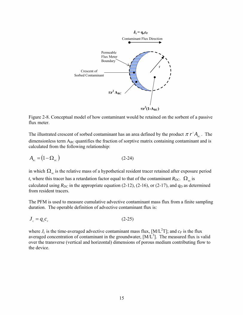
Figure 2-8. Conceptual model of how contaminant would be retained on the sorbent of a passive flux meter. The illustrated crescent of sorbed contaminant has an area defined by the product

RCAr 2π . The

dimensionless term ARC quantifies the fraction of sorptive matrix containing contaminant and is calculated from the following relationship:

(RCRC

A Ω−= 1 ) (2-24) in which is the relative mass of a hypothetical resident tracer retained after exposure period t, where this tracer has a retardation factor equal to that of the contaminant R

RCΩ

DC. is calculated using R

RCΩ

DC in the appropriate equation (2-12), (2-16), or (2-17), and qD as determined from resident tracers. The PFM is used to measure cumulative advective contaminant mass flux from a finite sampling duration. The operable definition of advective contaminant flux is:

FOCcqJ = (2-25)

where Jc is the time-averaged advective contaminant mass flux, [M/L2T]; and cF is the flux averaged concentration of contaminant in the groundwater, [M/L3]. The measured flux is valid over the transverse (vertical and horizontal) dimensions of porous medium contributing flow to the device.

15

Assuming the contaminant mass retained by the PFM, mc, is confined to a bulk volume of sorbent equaling bAr

RC

2π , the flux-average concentration of contaminant in the groundwater intercepted is:

DCRC

C

F RbArmcθπ 2

= (2-26)

Thus, combining equations (2-20), (2-25) equation (2-26) yields the following relationship for the time-averaged advective contaminant mass flux:

DCRC

CD

C RbArmqJθαπ 2

= (2-27)

where mc is the mass of contaminant sorbed, [M]; b is the length of sorptive matrix sampled or the vertical thickness of aquifer interval interrogated, [L]; and RDC as indicated previously is the retardation factor of contaminant for the sorbent. If it can be assumed that RDC is sufficiently large and that the hypothetical value of

RCΩ permits the application of equation (2-16), then it

may be assumed that and that equations (2-16), (2-25), and (2-27) may be combined to yield the following reduced equation for estimating time-averaged contaminant flux.

68.00 ≤<RC

A

rbtmJ C

C απ67.1

= (2-28)

Nonequilibrium contaminant sorption is not explicitly addressed in the above analysis nor is the occurrence of competitive sorption between contaminants and resident tracers. Competitive and rate-limited sorption undermine the efficiency of contaminant interception and retention on PFM sorbents. Hence, when either is significant, PFM measurements can underestimate true contaminant fluxes. Nonequilibrium contaminant sorption is most likely to occur when high groundwater velocities and/or small PFM diameters produce small Damkohler numbers (Bahr and Rubin 1987). A listing of key criteria used to design a flux meter is provided in Table 2.1. Primary consideration must be given to the desired sampling period (short- or long-term monitoring), the contaminant of interest, the nature of the sorbent to be used and the availability of non-toxic resident tracers with sufficiently large retardation factors. Assuming suitable sorbent and resident tracers exist, a flux meter can be designed using estimated permeabilities for the aquifer, the well screen and the sorbent (Klammler, et al. 2006a). Development of the flux meter and pertinent design criteria evolved from theoretical work initially submitted as part of a patent application made in October 1999 (Hatfield et al. 2002a).

16

Since that time, multiple laboratory experiments have been performed to validate theory and design prototypes of devices that could be demonstrated in the field. Some of the initial investigations were bench scales studies of flux meters using hexadecane as a sorbent; this work was extended by Hatfield et al. (2002b) to obtain consistent measurements of both water and contaminant fluxes in the laboratory. Several potential applications exist for the flux meter. Simultaneous measurements of water and contaminant flux have utility in long-term monitoring, aquifer restoration, natural attenuation, and contaminant source remediation. For example, in situ measurements of contaminant flux are needed to evaluate the strength of contaminant sources and to optimize the design and assess the performance groundwater remediation systems. Contaminant fluxes, when integrated over a source area, produce estimates of source strength and contaminant mass loads to groundwater and surface water.

]/[ TMLoaddydzJC =∫∫ (2-29)

Also, the flux average concentration [M/LfC 3] can be determine D

Cf q

JC = . Furthermore,

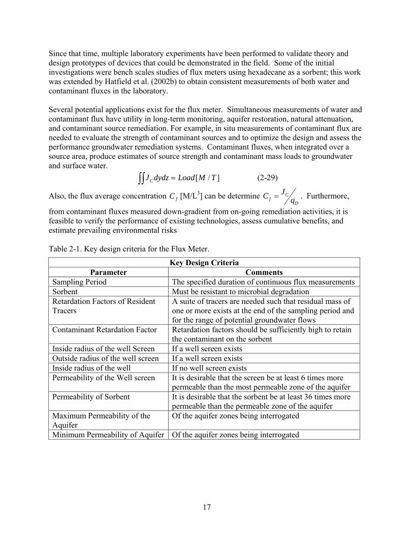
from contaminant fluxes measured down-gradient from on-going remediation activities, it is feasible to verify the performance of existing technologies, assess cumulative benefits, and estimate prevailing environmental risks Table 2-1. Key design criteria for the Flux Meter.

Key Design Criteria Parameter Comments

Sampling Period The specified duration of continuous flux measurements Sorbent Must be resistant to microbial degradation Retardation Factors of Resident Tracers

A suite of tracers are needed such that residual mass of one or more exists at the end of the sampling period and for the range of potential groundwater flows

Contaminant Retardation Factor Retardation factors should be sufficiently high to retain the contaminant on the sorbent

Inside radius of the well Screen If a well screen exists Outside radius of the well screen If a well screen exists Inside radius of the well If no well screen exists Permeability of the Well screen It is desirable that the screen be at least 6 times more

permeable than the most permeable zone of the aquifer Permeability of Sorbent It is desirable that the sorbent be at least 36 times more

permeable than the permeable zone of the aquifer Maximum Permeability of the Aquifer

Of the aquifer zones being interrogated

Minimum Permeability of Aquifer Of the aquifer zones being interrogated

17

2.2. Previous Testing of the Technology Significant prior testing of the technology has been limited to laboratory tests (Hatfield et al. 2002b and 2004). 2.3. Factors Affecting Cost and Performance The types of expenses typically associated with groundwater sampling are anticipated to exist with the flux measurements; these would include both direct and indirect environmental activity costs associated with sampling and analysis, labor, and training. For example, it is anticipated that comparable analytical costs will be incurred for each tracer or contaminant analyzed per sample. One cost that is unique to this technology is the cost associated with the flux meter sorbent (i.e., activated carbon or ion-exchange resin). Another important factor that could affect costs is the frequency of sampling. A flux meter provides time-integrated information in a single sample. The same type of information can be obtained through multiple water samples. It is expected that the long-term flux measurements will require less frequent sampling and fewer site visits. The final cost of concern is the number of analytes evaluated. With resident tracers the number of constituents analyzed will be greater than typical groundwater sampling. As indicated above the design and therefore the performance of the flux meter will depend on several factors. For example, knowing the permeability of the meter and having a good estimate of the aquifer permeability is essential. However, we show here that the PFM can be used to estimate aquifer permeability if local hydraulic gradients are measured while flux measurements are being taken. It is also important that the contaminant and some resident tracers have an affinity for the flux meter sorbent that is considered high but reversible; thus, the sorptive characteristics of the contaminant and resident tracers must be known. 2.4. Advantages and Limitations of the Technology The flux meter is the only technology available that provides simultaneous measurements of both water and contaminant fluxes. The prominent alternative technology is to quantify groundwater contaminant concentrations through multilevel samplers and then calculate contaminant fluxes using groundwater fluxes estimated from borehole dilution tests. The flux meter possess the advantage of providing a long-term monitoring solution that generates time integrated estimates of both groundwater and contaminant flux. Hence, transient fluctuations in contaminant concentrations and groundwater flows are not an issue of concern, as they are with traditional monitoring methods, because such variations are directly integrated in flux estimates. Field measurements do not require training beyond that currently needed in collecting groundwater samples. However, unlike typical groundwater sampling protocols wells used for flux measurements are not purged; thus, disposal of contaminated purge water is not an issue. Note that the duration of flux monitoring must be long enough that measurements are not significantly influence by hydraulic perturbation resulting from installation. Finally, the flux meter offer an additional advantage of not requiring power; thus, it can be used in remote

18

locations. Clearly, all other continuous monitoring technologies require power (such a down-hole flow meter). The primary limitation of the technology is that it could encourage the gathering of more samples at any single well, because it is quite easy to acquire multiple samples with depth (such as over the vertical extent of the well). Proper design of the flux meter should include aligning the vertical length of the sorbent material to cover the screen length of the well, so that samples acquired are representative of the depth intervals within the screen. A second limitation is that the method quantifies water fluxes by releasing resident tracer into the environment. Obtaining regulatory approval for the release of resident tracers could be time consuming. Selection of non-toxic, benign tracers could minimize permitting issues.

3.0. Demonstration Design

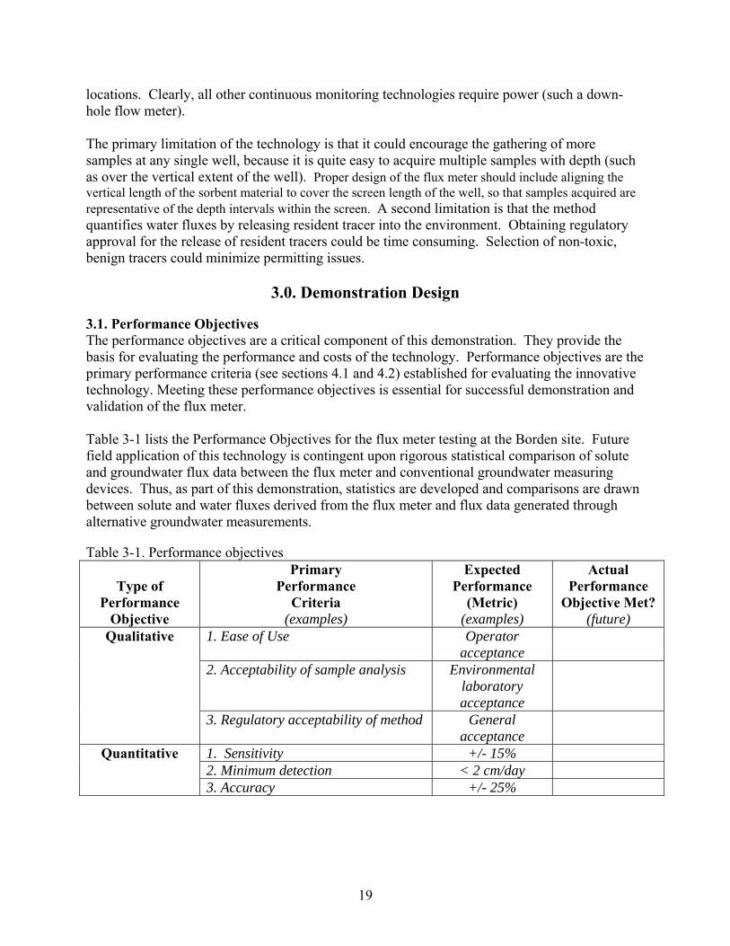
3.1. Performance Objectives The performance objectives are a critical component of this demonstration. They provide the basis for evaluating the performance and costs of the technology. Performance objectives are the primary performance criteria (see sections 4.1 and 4.2) established for evaluating the innovative technology. Meeting these performance objectives is essential for successful demonstration and validation of the flux meter. Table 3-1 lists the Performance Objectives for the flux meter testing at the Borden site. Future field application of this technology is contingent upon rigorous statistical comparison of solute and groundwater flux data between the flux meter and conventional groundwater measuring devices. Thus, as part of this demonstration, statistics are developed and comparisons are drawn between solute and water fluxes derived from the flux meter and flux data generated through alternative groundwater measurements.

Table 3-1. Performance objectives

Type of Performance

Objective

Primary Performance

Criteria (examples)

Expected Performance

(Metric) (examples)

Actual Performance

Objective Met? (future)

1. Ease of Use Operator acceptance

2. Acceptability of sample analysis Environmental laboratory acceptance

Qualitative

3. Regulatory acceptability of method General acceptance

1. Sensitivity +/- 15% 2. Minimum detection < 2 cm/day

Quantitative

3. Accuracy +/- 25%

19

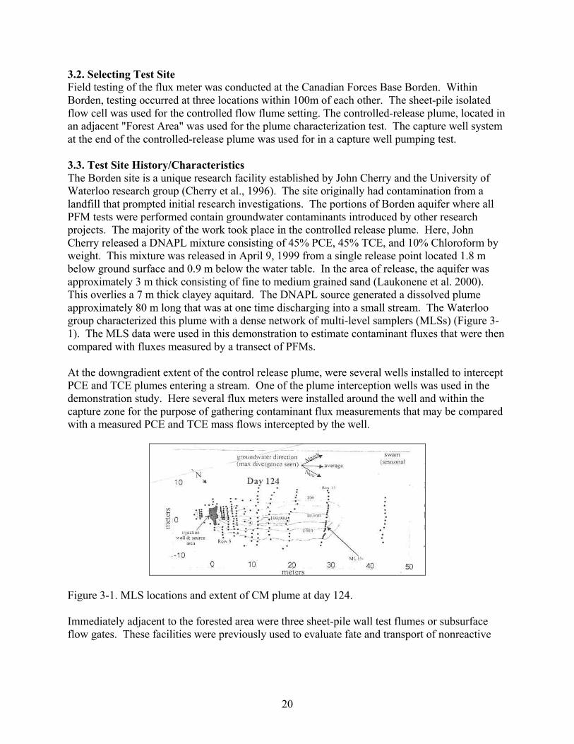
3.2. Selecting Test Site Field testing of the flux meter was conducted at the Canadian Forces Base Borden. Within Borden, testing occurred at three locations within 100m of each other. The sheet-pile isolated flow cell was used for the controlled flow flume setting. The controlled-release plume, located in an adjacent "Forest Area" was used for the plume characterization test. The capture well system at the end of the controlled-release plume was used for in a capture well pumping test. 3.3. Test Site History/Characteristics The Borden site is a unique research facility established by John Cherry and the University of Waterloo research group (Cherry et al., 1996). The site originally had contamination from a landfill that prompted initial research investigations. The portions of Borden aquifer where all PFM tests were performed contain groundwater contaminants introduced by other research projects. The majority of the work took place in the controlled release plume. Here, John Cherry released a DNAPL mixture consisting of 45% PCE, 45% TCE, and 10% Chloroform by weight. This mixture was released in April 9, 1999 from a single release point located 1.8 m below ground surface and 0.9 m below the water table. In the area of release, the aquifer was approximately 3 m thick consisting of fine to medium grained sand (Laukonene et al. 2000). This overlies a 7 m thick clayey aquitard. The DNAPL source generated a dissolved plume approximately 80 m long that was at one time discharging into a small stream. The Waterloo group characterized this plume with a dense network of multi-level samplers (MLSs) (Figure 3-1). The MLS data were used in this demonstration to estimate contaminant fluxes that were then compared with fluxes measured by a transect of PFMs. At the downgradient extent of the control release plume, were several wells installed to intercept PCE and TCE plumes entering a stream. One of the plume interception wells was used in the demonstration study. Here several flux meters were installed around the well and within the capture zone for the purpose of gathering contaminant flux measurements that may be compared with a measured PCE and TCE mass flows intercepted by the well.

Figure 3-1. MLS locations and extent of CM plume at day 124. Immediately adjacent to the forested area were three sheet-pile wall test flumes or subsurface flow gates. These facilities were previously used to evaluate fate and transport of nonreactive

20

tracers, MTBE, and chlorinated solvents. For this demonstration gate 2 was used to evaluate PFM performance under known ground water flow rates. Both groundwater and MTBE fluxes were measured and results compared with known groundwater flows and MTBE flux estimates given by available MLS. 3.4. Present Operations Currently the only active operations of interest are the pump and treat capture system at the end of the controlled release plume and the ongoing MLS monitoring of the plume. This plume interception system has been operational approximately since 2000 and was instituted to stop a contaminant discharge to a small stream. This system consists of three capture wells that are pumped continuously in order to capture the entire width of the plume. 3.5. Pre-Demonstration Testing and Analysis All the sites were characterized by the Waterloo research group. Research personnel needed only to install the flux meters for the given test and then retrieved them after a specified period of exposure to the groundwater flow field. 3.6. Testing and Evaluation Plan

3.6.1. Demonstration Set-Up and Start-Up Prior to any field experiments, several laboratory batch experiments were conducted to select sorbents and tracers. In addition, flow-through-box aquifer experiments were executed under known flow conditions to characterize the performance of the flux meter under controlled water and contaminant flux conditions. Solid-aqueous phase batch partitioning tests were performed as a preliminary evaluation of potential PFM sorbents for intercepting contaminants (PCE and TCE) and releasing tracers. Activated carbon was the primary sorbent under consideration, because it was inexpensive, and it could be recycled. Batch tests followed well-established methods for determining sorption and desorption isotherms between solid and aqueous phases. Measured isotherms were used to assess the applicability of each sorbent as a packing media for the flux meter. Whether the sorption/desorption isotherm was linear or nonlinear appropriate partitioning coefficients were determined for flux meter. Hysteretic and non-equilibrium partitioning behavior were also considered in the sorbent and tracer selection process. Flow-through-box aquifer experiments conducted under known flow conditions were used to characterize the performance of PFMs in screened wells. A water-tight container (stainless steel) with dimensions of ~27 cm by ~20 cm and ~18 cm deep was used to create the aquifer model. The two ends of the container were packed with course gravel to serve as permeable sections for flow injection and extraction. This was done to provide a constant head across the width of the box, and a uniform gradient along the length of the box. The main section of the box was packed under water with sand to a height of 13.1 cm. The sand used was from the test site at CFB Borden. Placed inside the box was a 5.1 cm (2 inch) well screen as the sand was packed. The water used in packing the sand and later used to produce flow through the box aquifer contained

21

one surrogate contaminants (2,4-dimethyl-3-pentanol). The water table in the box was set to a height of 13.1 cm. Because silver impregnated activated carbon was determined to be the most suitable PFM sorbent, the meters were constructed as simply activated carbon packed in permeable nylon or cotton socks. The carbon was pre-equilibrated with several resident tracers. To conduct a flux measurement, the flux meters were inserted into the well screen where they were then exposed to the porous flow in the box. Following a specified duration of exposure, the meters were pulled from the well screen and the activated carbon extracted to measure the masses of surrogate contaminants intercepted and the masses of resident tracers loss. To conduct flux monitoring in the field, 3.2 or 5.1 cm fully screened PVC monitoring wells were used. For example, when flux monitoring of the controlled release plume was conducted, a single transect of flux wells was installed immediately downgradient from MLS transect 13. Seventeen 3.2 or 5.1 cm shallow fully-screened monitoring wells were installed in which flux meters were later inserted. The wells were installed using standard techniques supported by the Waterloo group and without sand packs which allowed the formation to collapse around the well screens. For the field test involving the plume interception well, eight 3.2 cm fully-screened monitoring wells were installed to encompass the capture zone of the interception well. Again, these shallow wells were installed using standard techniques, and again PFM’s were inserted into these wells when fluxes were being measured. In the controlled flow system, two transects of three 5.2 cm fully-screened wells were installed. In one transect screens were installed with 2.54 cm sand packs. The idea here was draw comparisons between water and contaminant fluxes measured in wells with and without sand packs. Before any well was used for flux measurements, it was developed (usually immediately after installation) and then left for approximately one week to equilibrate with the flow field before a PFM was inserted. All materials needed for constructing PFM’s and for subsequent sampling were transported to Borden prior to the field activities. Required materials included resident tracers, sorbent, sock material, threaded rod and pipe. Additional equipment needs included, a balance, graduated cylinders, mixing containers, sample vials and extraction solvents. Each PFM was constructed on-site and then immediately inserted in a selected well. Tracers used were in some cases volatile and therefore the time between construction and insertion was kept to a minimum. The construction of each flux device involved packing the carbon sorbent (with tracers) with multiple impermeable dividers in a sock. Each PFM of 1.5m length required about 30 minutes to construct and install. As many as 25 PFMs were installed in 17 wells to characterize fluxes over a single transect of the controlled-release plume. One day was required to complete the installation. Prior to each flux monitoring event, University of Waterloo would gather water samples from MLS wells located immediately upgradient from where the flux meters were installed. The PFMs remained in the field from 3 days to 6 weeks depending on the experiment. In most cases personnel left the site only to return at a later date for PFM retrieval. During retrieval, the

22

PFM was removed from the well and segmented vertically for sorbent sub-sampling. Each 20-25 cm interval of sorbent was homogenized and sub-sampled for analysis. The process of extraction and subsampling required about 20 minutes per meter. Approximately 8 hours were required to sample all 25 PFMs deployed to characterize the plume near MLS transect 13.

3.6.2. Period of Operation The work at the Borden site was carried out over a period of 18 months and then when weather permitted. Experiments involving the extraction well were conducted in May and November 2001. The controlled flume experiment was executed in August of 2002. Finally, PFM testing in the control release plume was performed twice, once in April and then again in late August of 2002.

3.6.3. Amount /Treatment Rate of Material to be Treated Not applicable.

3.6.4. Residuals Handling Flux meters generate a minimal amount of waste. The largest test involved 25 flux meters that were 3.2 cm in diameter and 1.5 m long. This experiment produced approximately 30 liters (8 gallons) of residual sorbent containing tracers and contaminants. This waste was stored on-site in drums for later disposal by the Waterloo research group.

3.6.5. Operating Parameters for the Technology Operationally the flux meter is very simple. This is one of the advantages of the technique. A single individual can perform the method; however, two is likely the best operationally. The device can be installed in a number of wells (10 to 20) in a single day. The extraction is quite simple and again could be conducted by a single individual. PFMs require no electrical utilities and can be performed in remote locations. An electronic balance is used before and after sampling; however, these measurements can be made in the laboratory.

3.6.6. Experimental Design The focus of this research effort was to demonstrate/validate the PFM using three field experiments as described earlier. Each experiment was designed to provide independent estimates of both groundwater and contaminant fluxes which could be compared to fluxes measured by PFMs. The first set of field experiments were conducted at Borden using an existing sheet-pile enclosed flume for flow gate. The flume was 15-m long and 2 m wide and opened on one end. The saturated thickness of the aquifer is about 1.5 m. Flow was established from one pumping well located in the closed end of the flume. Steady one-dimensional flow was maintained throughout the period of the field experiment. Flow rates and contaminant concentrations were monitored at intervals that provide accurate estimates of flow and average contaminant concentrations. Two sets of three PFMs were installed in 5.1 cm fully-screen wells for a period of approximately one week. Three PFMs were installed wells constructed with sand packs and three without. PFM measured water fluxes were compared with the flux calculated from the measured flow rate of

23

the extraction well. PFM measured MTBE fluxes were compared to fluxes estimated from MTBE concentrations measured in the six flux wells and from an existing network of MLS. The second field experiment involved monitoring fluxes in a TCE/PCE plume generated from a previous controlled-release experiment. Here, a dense network of multilevel samplers was installed to characterize the plume as it developed. Approximately 20 sampling transects were installed to completely characterize the width of the plume at various distances from the source. The focus of the field experiment was to monitor fluxes immediately down gradient from the 13th

MLS transect. Seventeen fully screen 3.2 cm monitoring wells were installed one meter down gradient from the 13th MLS transect. As many as 25 PFMs were inserted in these wells for monitoring durations ranging from 4 to 6 weeks. As water, PCE, and TCE fluxes were monitored, water table measurements were taken from other wells and water samples were collected from MLS from the 13th transect. The gathered MLS data and water table elevations were used to estimate both the hydraulic gradient and the flow of groundwater and the TCE/PCE fluxes in the plume. These estimated fluxes were compared to the values measured by the flux meters. In the last experiment, PFM were used to measure water, PCE, and TCE fluxes within the capture zone of a plume interception well. A ring of eight 3.2 cm fully screened monitoring wells were placed within the capture zone of a well originally design to intercept the TCE/PCE plumes generated from the controlled release experiment conducted in the Forested Area of the Borden test facility. The eight monitoring wells were evenly apart at a radial distance of 35 cm from the active interception well. Groundwater flow and contaminant fluxes measured by PFMs were compared to measured water flows and calculated contaminant mass flows. Contaminant concentrations and flows measured at the well head were used to calculate contaminant mass flows over the 3-day test.

3.6.7. Sampling Plan The PFM demonstration/validation experiments focused on a sampling density that was adequate to provide a reasonable comparison to the fluxes measured or estimated by other means. For characterizing the controlled release plume, horizontal spacing of PFMs and vertical sampling of PFM sorbent corresponded with the MLS network density. PFMs were space horizontally at 1 m intervals; whereas, the vertical resolution of sorbent sampling was 20 to 25 cm. Sampling within the controlled flow flume will use 0.5 m spacing and 10 cm vertical resolution over the entire saturated zone. Two rows of wells were deployed. Extraction well flow rates were measured twice a day and water samples were be collected once a day during the flux meter installation. For the experiment comparing PFM measured fluxes with those derived from the plume interception well, a vertical sampling resolution of 10 cm was used over the entire saturated zone. Twice daily the interception well flow rate was measured and water samples were gathered for subsequent TCE/PCE analyses.

24

Sample Collection. Two types of samples were collected during this study, groundwater samples from MLSs or extraction wells, and sorbent samples from flux meters. Water samples were collected in EPA VOA vials with zero headspace. Samples will be drawn by syringe from the MLSs and collected at outflow lines from the extraction wells. Sampling protocol at the Borden site will follow recommend methods from the University of Waterloo research group to be consistent with prior data collection (Broholm, Feenstra, and Cherry, 1999). These samples were immediately placed in coolers and maintained cold during overnight shipping to Florida. These samples were held for less than two weeks prior to analysis. Samples were analyzed for MTBE, PCE, TCE and CF. Sorbent samples were collected from the extracted flux meters. 10 cm or 20 to 25 cm vertical intervals of PFM sorbent were segmented and transferred to containers for homogenization. Samples were stirred and subsampled into 40-ml VOA vials containing an extraction fluid isobutyl alcohol (IBA). Approximately 10 grams of sorbent were be extracted with 40 ml of IBA. These samples will be cooled for shipping to Florida and will be analyzed within two weeks. Sample Analysis. All samples were analyzed at laboratories at the University of Florida or Purdue University. Volatile organics, including alcohol tracers, were analyzed by direct liquid injection on Gas Chromatographs. Details of analytical methods wew provided in Appendix A. Detection limits were approximately 1 mg/L. Headspace analysis was used in the event that low concentrations were encountered. Detection limits for headspace analysis was approximately 50 ug/L Experimental Controls. The University of Waterloo group monitored the controlled release plume using the available MLS network. The monitoring data were used to calculate contaminant fluxes for subsequent comparisons to results derived from flux meters. Data Quality Parameters. Data quality will be maintained and checked throughout the project. Details on approaches for maintaining data quality are provided in the QA/QC plan in appendix C. Calibration Procedures, Quality Control Checks, and Corrective Action. Initial and continuing calibration procedures for analytical instrumentation, quality control checks, and corrective actions were conducted to maintain reproducible experiments. These procedures were fully described in the QA/QC plan in appendix C. Data Quality Indicators. Simple regression analysis was used to assess the quality of data collected at any single well. However, more sophisticated techniques of spatial analysis were performed with data collected to assess the spatial mean and variance of contaminant and water fluxes evaluated over transects or within a plume.

25

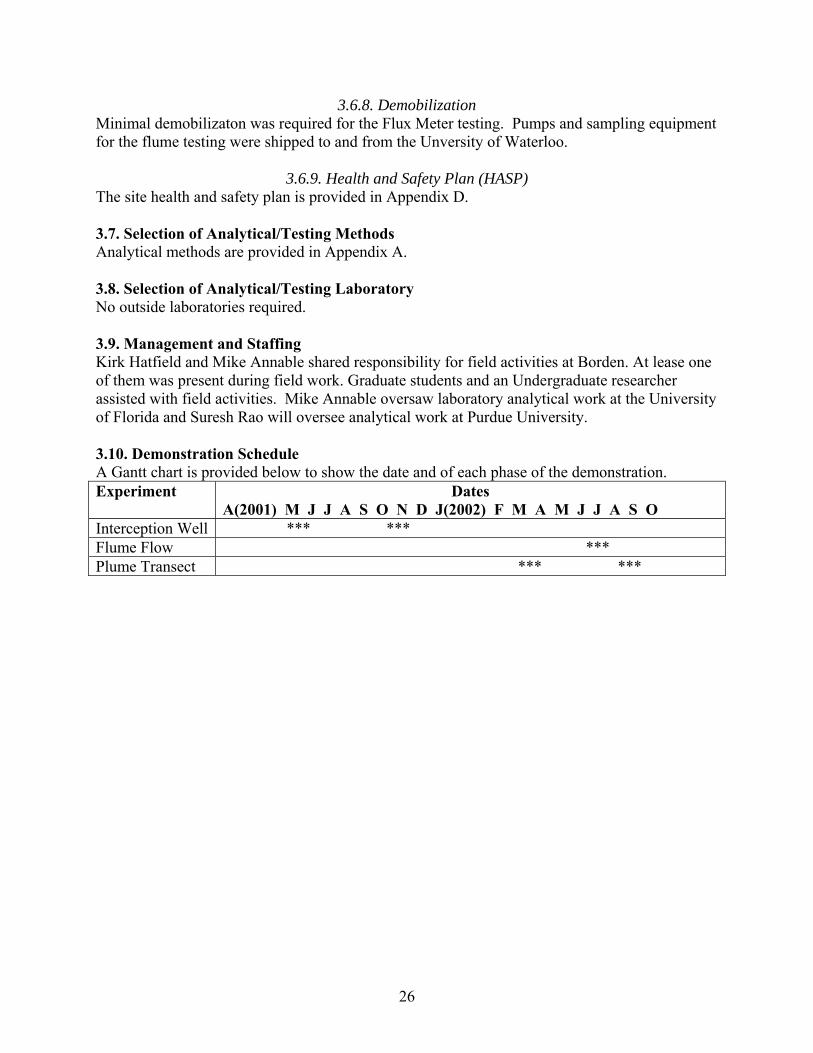
3.6.8. Demobilization Minimal demobilizaton was required for the Flux Meter testing. Pumps and sampling equipment for the flume testing were shipped to and from the Unversity of Waterloo.

3.6.9. Health and Safety Plan (HASP) The site health and safety plan is provided in Appendix D. 3.7. Selection of Analytical/Testing Methods Analytical methods are provided in Appendix A. 3.8. Selection of Analytical/Testing Laboratory No outside laboratories required. 3.9. Management and Staffing Kirk Hatfield and Mike Annable shared responsibility for field activities at Borden. At lease one of them was present during field work. Graduate students and an Undergraduate researcher assisted with field activities. Mike Annable oversaw laboratory analytical work at the University of Florida and Suresh Rao will oversee analytical work at Purdue University. 3.10. Demonstration Schedule A Gantt chart is provided below to show the date and of each phase of the demonstration. Experiment Dates

A(2001) M J J A S O N D J(2002) F M A M J J A S O Interception Well *** *** Flume Flow *** Plume Transect *** ***

26

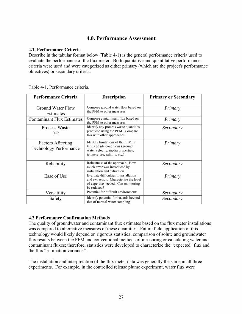
4.0. Performance Assessment

4.1. Performance Criteria Describe in the tabular format below (Table 4-1) is the general performance criteria used to evaluate the performance of the flux meter. Both qualitative and quantitative performance criteria were used and were categorized as either primary (which are the project's performance objectives) or secondary criteria.

Table 4-1. Performance criteria.

Performance Criteria Description Primary or Secondary

Ground Water Flow Estimates

Compare ground water flow based on the PFM to other measures.

Primary

Contaminant Flux Estimates Compare contaminant flux based on the PFM to other measures.

Primary

Process Waste (all)

Identify any process waste quantities produced using the PFM. Compare this with other approaches

Secondary

Factors Affecting Technology Performance

Identify limitations of the PFM in terms of site conditions (ground water velocity, media properties, temperature, salinity, etc.)

Primary

Reliability

Robustness of the approach. How much error was introduced by installation and extraction.

Secondary

Ease of Use

Evaluate difficulties in installation and extraction. Characterize the level of expertise needed. Can monitoring be reduced?

Primary

Versatility Potential for difficult environments. Secondary Safety Identify potential for hazards beyond

that of normal water sampling Secondary

4.2 Performance Confirmation Methods The quality of groundwater and contaminant flux estimates based on the flux meter installations was compared to alternative measures of these quantities. Future field application of this technology would likely depend on rigorous statistical comparison of solute and groundwater flux results between the PFM and conventional methods of measuring or calculating water and contaminant fluxes; therefore, statistics were developed to characterize the “expected” flux and the flux “estimation variance”. The installation and interpretation of the flux meter data was generally the same in all three experiments. For example, in the controlled release plume experiment, water flux were

27

compared with estimates based on recent borehole dilution tests performed immediately prior to or immediately following flux meter measurements. Contaminant flux, however, were compared with estimates based on multilevel sampler data collected during the flux meter placement period. Use of multilevel sampler data alone could only provide an estimate of TCE and PCE fluxes since assumptions had to be made regarding the hydraulic conductivity field across the section of interest and the hydraulic gradient. Table 4-2 lists for each performance criterion an expected or a desired value and the method that would be used to confirm performance such that the performance of the flux meter could be assessed as acceptable or not. Qualitative metrics were selected for several performance criteria including: ease of use (a primary criterion), reliability, safety, and versatility. Ease of use was an important performance criterion and it was expected that the results of the demonstration would document the level of training required to install/extract and interpret information from the flux meter. Reliability was assessed from records of total device installations verses total numbers of device failures. The performance metrics for the versatility criterion werel a demonstration that the flux meter was successfully applied to generate both short- and long-term assessments, and that it could be applied (in theory) to other sorbing (or ion exchanging) contaminants (e.g., metals, radionuclides). As indicated in table 4.2, several quantitative performance metrics were identified to assess the performance of the new technology. Because the typical range for contaminant fluxes in the field could be 5 orders of magnitude (for water fluxes the range was 2 orders of magnitude), it is believed that achieving the performance metrics identified would greatly reduce the uncertainty of contaminant flux assessments. Clearly, a significant uncertainty reduction would be valuable to regulators and site managers. For the plume experiments discussed above, a successful comparison would results if the groundwater and contaminant fluxes were estimated within 20 and 35% respectively. The higher uncertainty associated with contaminant flux measurements was allowed due to the nature of the MLS based estimates. In the flume and the extraction well experiments, water and contaminant flux were known with more certainty. Acceptable comparisons with the flux meter results were set at 15 and 25% for groundwater and contaminant flux respectively.

28

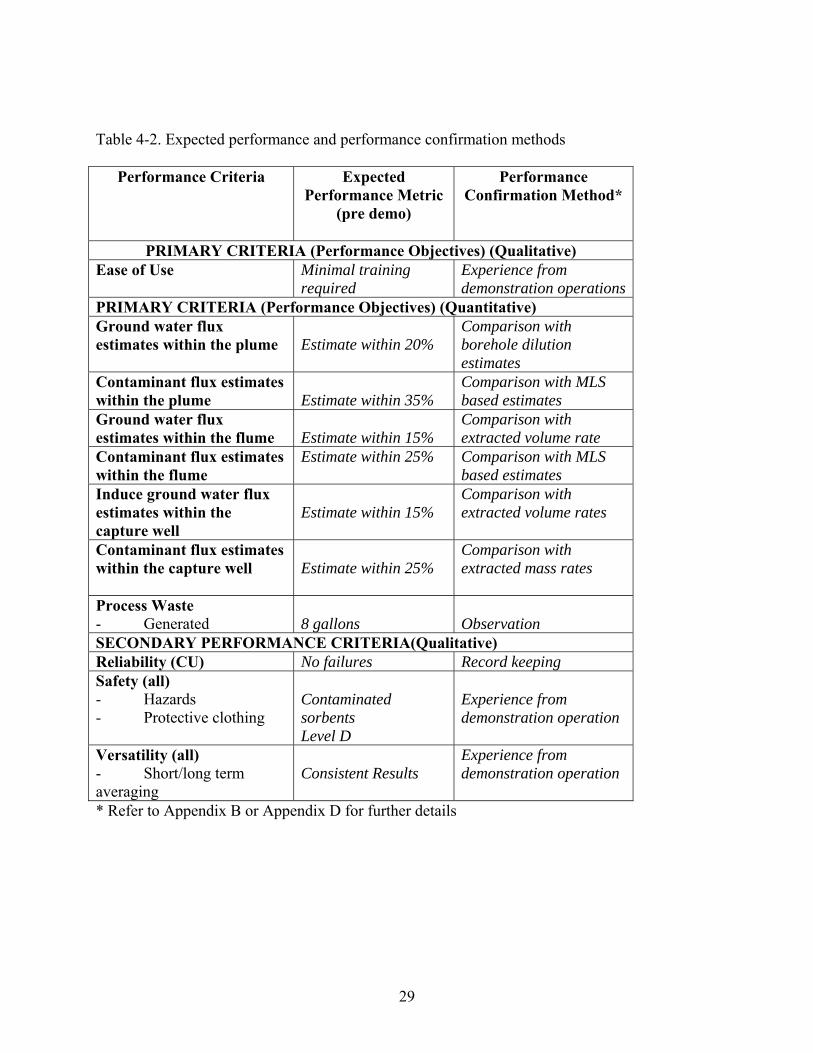
Table 4-2. Expected performance and performance confirmation methods

Performance Criteria

Expected Performance Metric

(pre demo)

Performance Confirmation Method*

PRIMARY CRITERIA (Performance Objectives) (Qualitative) Ease of Use Minimal training

required Experience from demonstration operations

PRIMARY CRITERIA (Performance Objectives) (Quantitative) Ground water flux estimates within the plume

Estimate within 20%

Comparison with borehole dilution estimates

Contaminant flux estimates within the plume

Estimate within 35%

Comparison with MLS based estimates

Ground water flux estimates within the flume

Estimate within 15%

Comparison with extracted volume rate

Contaminant flux estimates within the flume

Estimate within 25% Comparison with MLS based estimates

Induce ground water flux estimates within the capture well

Estimate within 15%

Comparison with extracted volume rates

Contaminant flux estimates within the capture well

Estimate within 25%

Comparison with extracted mass rates

Process Waste - Generated

8 gallons

Observation

SECONDARY PERFORMANCE CRITERIA(Qualitative) Reliability (CU) No failures Record keeping Safety (all) - Hazards - Protective clothing

Contaminated sorbents Level D

Experience from demonstration operation

Versatility (all) - Short/long term averaging

Consistent Results


* Refer to Appendix B or Appendix D for further details

29

4.3. Data Analysis, Interpretation and Evaluation Section 4.3.1 begins with a presentation of results from several bench-scale aquifer experiments. These experiments permit an evaluation of the PFM performance under known conditions. Next, in section 4.3.2 results from three field demonstrations this are presented and discussed.

4.3.1. Laboratory Experiments Experimental Design Laboratory box aquifer experiments were conducted to evaluate the PFM. Experiments involved placement of meters in a box aquifer such that measurements of cumulative water and contaminant fluxes could be made. Granular activated carbon (Fisher Scientific, 6-12 mesh) was the sorbent used in the meters. The carbon had a mean grain size of 2 mm and a hydraulic conductivity of 0.59 cm/s. The packed carbon porosity and dry bulk density were respectively 0.62 and 0.552 g/cm3. Ethanol, methanol, isopropyl alcohol, and n-hexanol served as resident tracers pre-equilibrated on the activated carbon. A branched alcohol, 2,4-dimethyl-3-pentanol (DMP) functioned as a surrogate aquifer contaminant. A stainless steel container (Cole-Parmer, 27 x 20 x 18 cm deep) was used to create the box aquifer. A 16 cm section of well screen (5.24 cm I.D. and 5.87 cm O.D.) was positioned upright and in the center of box. The box was packed with sand (under standing water) to a height of 13.1 cm and then overlaid with 2-3 cm of saturated bentonite. The sand was commercial grade medium grain size having a hydraulic conductivity of 0.01 cm/s. The two ends of the container were used for flow injection and extraction and were packed with coarse gravel (8 mm mean gain diameter). This was done to provide a constant head across the width of the box, and a uniform gradient across the length of the box. The phreatic surface was set to a height of 13.1 cm and the applied flow rate ranged from 0.78 to 4.7 ml/min giving a Darcy flux from 0.20 to 1.19 cm/hr. The total depth of water in the well, , was maintained at 12.6 cm, and it extended 0.5 cm from bottom of the box to an elevation of 13.1 cm. Within the water saturated interval the slotted screen length, , equaled 12.1 cm.

Wl

Sl

PFMs were pre-equilibrated, wet, activated carbon packed into crinoline socks. Pre-equilibration constituted 24 hours of gently mixing 320 g of dry activated carbon in a 2 L aqueous solution containing 1.18 g ethanol, 1.19 g methanol, 2.36 g isopropyl alcohol, and 2.44 g n-hexanol. The cotton crinoline socks were 16 cm long and 5.24 cm in diameter and were pre-washed in water. Each sock was packed to contain approximately 150 g of activated carbon (dry mass); this produced a PFM with a length that typically ranged from 13.3 to 13.5 cm. During the construction of each PFM, the activated carbon was sampled to establish initial concentrations of the sorbed resident tracers. These concentrations were used in subsequent calculations to ascertain ΩR, the relative mass of each tracer remaining in the PFM following a period of exposure to flow in the box aquifer.

30

Preceding each box experiment, DMP influent/effluent concentrations were measured to verify that initial contaminant conditions were quasi-steady-state. Among the several experiments conducted, influent DMP concentrations ranged from 72.0 to 83.0 mg/l and produced quasi-steady-state box aquifer effluent concentrations ranging from 72.0 to 77.5 mg/L. During each experiment, a meter was inserted into the well screen and influent/effluent concentrations of DMP were monitored. Because the PFM was designed to intercept and retain DMP, box-aquifer effluent concentrations inevitably decreased to new quasi-steady-state levels, which again among the several experiments ranged from 44.0 to 49.5 mg/L. After a desired period of exposure, the meter was pulled and the carbon sampled for subsequent resident tracer and contaminant analyses. Between experiments, constant flow through the box aquifer was maintained to re-establish DMP effluent concentrations representing quasi-steady-state initial conditions. Sampling of the PFM involved extracting the activated carbon with isobutyl alcohol. From the extract all resident tracers and DMP were analyzed using a Perkin-Elmer Gas Chromatograph (GC) equipped with automated liquid injection and a Flame Ionization detector (FID). n-hexanol has an aqueous/activated-carbon retardation factor in excess of 8000; thus, it functionally behaves as a non-desorbing resident tracer as compared to methanol, isopropyl alcohol, and ethanol. n-hexanol was used as an internal standard whereby changes in RΩ for methanol, isopropyl alcohol, and ethanol were assessed from measured changes in tracer mass ratios with respect to n-hexanol. Measured values of RΩ were used in equations (2-17) and (2-23) to determine local water fluxes and compared to known experimental water fluxes. Mass measurements of DMP intercepted and retained on activated carbon, m

oqC , were used in equation

(2-28) to obtain measured cumulative contaminant fluxes, these were subsequently compared to experimental fluxes imposed on the system. In support of the box aquifer experiments, ancillary experiments were conducted to ascertain the resident tracer elution functions ( )τG and to quantify the well screen permeability. Resident tracer elution functions were derived from a column elution experiment. Glass columns 5 cm long and 2.4 cm inside diameter were packed with 11.8 grams (expressed as dry weight) of activated carbon that had been prequilibrated as described above with ethanol, methanol, isopropyl alcohol, and n-hexanol. The column was then eluted with water at a flow rate of 0.5 (ml/min). Frequent volumetric measurements were taken to develop plots of cumulative elution volume versus time. Whenever the eluent volume was measured, a sample was collected analyzed to assess transient changes in dissolved concentrations of resident tracers and DMP. The dissolved constituent concentrations were determined by direct injection of the eluent sample on a Perkin-Elmer GC with FID. To estimate the well screen hydraulic conductivity, it was necessary to conduct a borehole dilution test (Drost et al., 1968) in the box aquifer well where flow was known; however, this approach should not be construed as a method for determining screen permeabilities in the field. The test required a few drops of concentrated NaCl solution and use of an electrical conductivity meter (Orion Model 115Aplus). Initially, the ambient electrical conductivity of water in the box

31

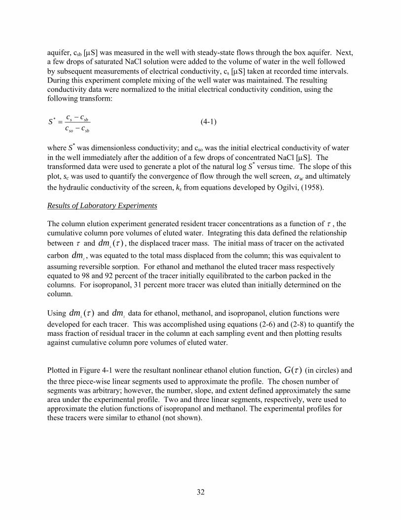
aquifer, csb [µS] was measured in the well with steady-state flows through the box aquifer. Next, a few drops of saturated NaCl solution were added to the volume of water in the well followed by subsequent measurements of electrical conductivity, cs [µS] taken at recorded time intervals. During this experiment complete mixing of the well water was maintained. The resulting conductivity data were normalized to the initial electrical conductivity condition, using the following transform:

sbso

sbs

ccccS

−−

=* (4-1)

where S* was dimensionless conductivity; and cso was the initial electrical conductivity of water in the well immediately after the addition of a few drops of concentrated NaCl [µS]. The transformed data were used to generate a plot of the natural log S* versus time. The slope of this plot, sc was used to quantify the convergence of flow through the well screen, Wα and ultimately the hydraulic conductivity of the screen, ks from equations developed by Ogilvi, (1958). Results of Laboratory Experiments The column elution experiment generated resident tracer concentrations as a function of τ , the cumulative column pore volumes of eluted water. Integrating this data defined the relationship between τ and )(τ

Ldm , the displaced tracer mass. The initial mass of tracer on the activated

carbon , was equated to the total mass displaced from the column; this was equivalent to assuming reversible sorption. For ethanol and methanol the eluted tracer mass respectively equated to 98 and 92 percent of the tracer initially equilibrated to the carbon packed in the columns. For isopropanol, 31 percent more tracer was eluted than initially determined on the column.

Idm

Using )(τ

Ldm and data for ethanol, methanol, and isopropanol, elution functions were

developed for each tracer. This was accomplished using equations (2-6) and (2-8) to quantify the mass fraction of residual tracer in the column at each sampling event and then plotting results against cumulative column pore volumes of eluted water.

Idm

Plotted in Figure 4-1 were the resultant nonlinear ethanol elution function, )(τG (in circles) and the three piece-wise linear segments used to approximate the profile. The chosen number of segments was arbitrary; however, the number, slope, and extent defined approximately the same area under the experimental profile. Two and three linear segments, respectively, were used to approximate the elution functions of isopropanol and methanol. The experimental profiles for these tracers were similar to ethanol (not shown).

32

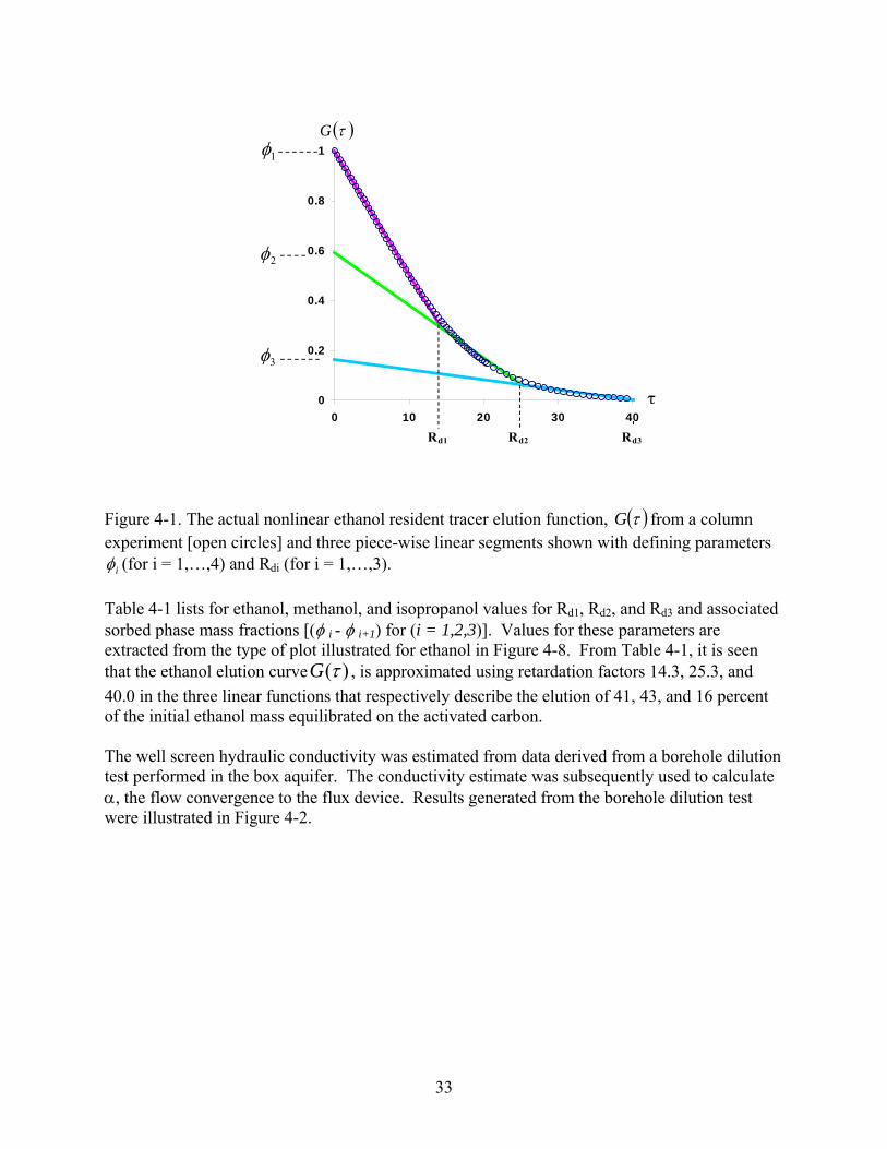
0

0.2

0.4

0.6

0.8

1

0 10 20 30 40

τ

( )τG

Rd1 Rd2 Rd3

1φ

2φ

3φ

Figure 4-1. The actual nonlinear ethanol resident tracer elution function, ( )τG from a column experiment [open circles] and three piece-wise linear segments shown with defining parameters

iφ (for i = 1,…,4) and Rdi (for i = 1,…,3). Table 4-1 lists for ethanol, methanol, and isopropanol values for Rd1, Rd2, and Rd3 and associated sorbed phase mass fractions [(φ i - φ i+1) for (i = 1,2,3)]. Values for these parameters are extracted from the type of plot illustrated for ethanol in Figure 4-8. From Table 4-1, it is seen that the ethanol elution curve )(τG , is approximated using retardation factors 14.3, 25.3, and 40.0 in the three linear functions that respectively describe the elution of 41, 43, and 16 percent of the initial ethanol mass equilibrated on the activated carbon. The well screen hydraulic conductivity was estimated from data derived from a borehole dilution test performed in the box aquifer. The conductivity estimate was subsequently used to calculate α, the flow convergence to the flux device. Results generated from the borehole dilution test were illustrated in Figure 4-2.

33

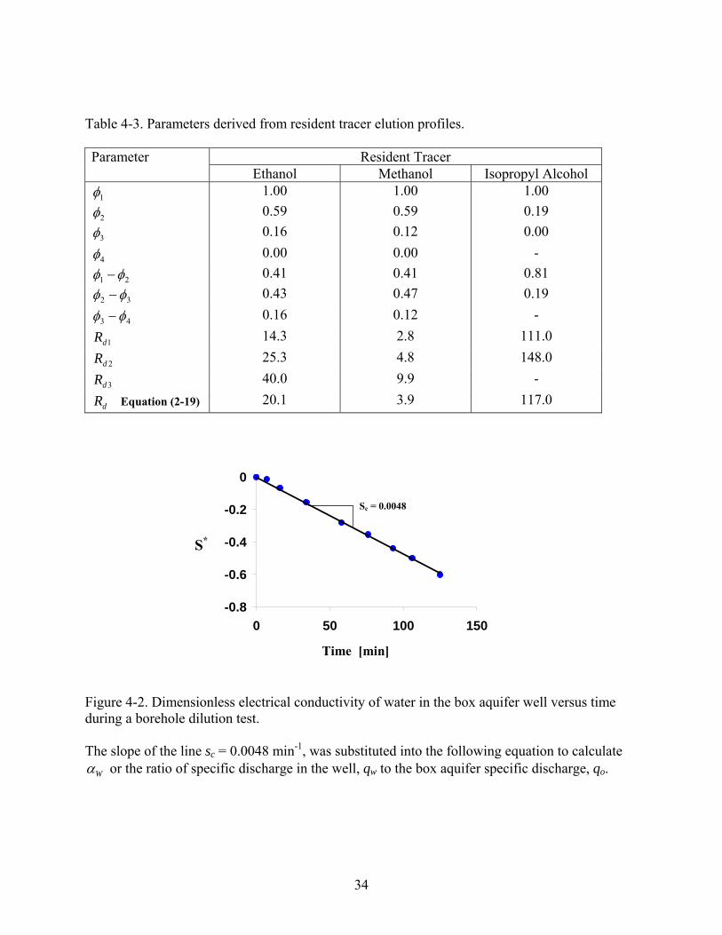
Table 4-3. Parameters derived from resident tracer elution profiles.

Resident Tracer Parameter Ethanol Methanol Isopropyl Alcohol

1φ 1.00 1.00 1.00

2φ 0.59 0.59 0.19

3φ 0.16 0.12 0.00

4φ 0.00 0.00 -

21 φφ − 0.41 0.41 0.81

32 φφ − 0.43 0.47 0.19

43 φφ − 0.16 0.12 -

1dR 14.3 2.8 111.0

2dR 25.3 4.8 148.0

3dR 40.0 9.9 -

dR Equation (2-19) 20.1 3.9 117.0

-0.8

-0.6

-0.4

-0.2

0

0 50 100 150

S*

Time [min]

Sc = 0.0048

Figure 4-2. Dimensionless electrical conductivity of water in the box aquifer well versus time during a borehole dilution test. The slope of the line sc = 0.0048 min-1, was substituted into the following equation to calculate

Wα or the ratio of specific discharge in the well, qw to the box aquifer specific discharge, qo.

34

( )ow

pwc

o

WW qrl

rlsqq

2

2 ∀−==

πα (4-2)

where represented the volume of the electrical conductivity probe, [Lp∀ 3]. Equation (4-2) was derived from Drost et al., (1968). During the experiment, the imposed flow was 0.011 cm/min. Parameters r and lw were respectively 2.62 and 12.6 cm. The displacement volume of the conductivity probe, measured 41 cmp∀ 3. Using the aforementioned parameter values in equation (4-2) yielded a value of 1.55 for Wα . From Wα , a well screen hydraulic conductivity of 0.0027 cm/s was calculated using equation (31), which was derived from Ogilvi, (1958) and Drost et al., (1968).

Sk

( )

( )WWS

SWO

S RRkk

ααα

−−−

=4

12

2

(4-3)

For this calculation, the assumed aquifer hydraulic conductivity, was 0.01 cm/s; while 1.12 and 1.55 were the respective dimensionless values of R

okS and Wα .

With the well screen hydraulic conductivity known, a direct determination was made of α. Using equation (2-22) a value of 1.53 was calculated for the flow convergence parameter. This value of α essentially predicted that resident tracers would be displaced and that contaminant mass would be intercepted at rates consistent with contaminant fluxes and specific discharges that were 53% greater inside the PFM than in the surrounding porous media. Tracer results from multiple PFM experiments are shown in Figure 4-3. The plot illustrates the mass fraction of residual tracer measured in each PFM versusξ . Equations (2-15) and (2-17) are also plotted for comparison; although values from equation (2-17) reflect parameter values for ethanol alone (see Table 4-3). An evaluation of equation (2-17) using parameter values for isopropanol is not necessary, because cumulative fluxes are sufficiently small that calculated ξ ’s are less than 0.15 and therefore within the applicable range of equation (2-15). For the most part, resident tracers are displaced at rates linearly related to the cumulative volume of water intercepted. Figure 4-3 illustrates the claim that equation (2-15) can be used for all tracers and in lieu of (2-17) whenever the relative mass retained is within the range of

. However, as demonstrated for the ethanol tracer, equation (2-17) describes the relationship between residual tracer mass and cumulative groundwater flux when measured groundwater flows result in

00.132.0 ≤Ω≤R

ξ values greater than 0.56 or reduce resident tracer masses to relative values less than 0.32.

35

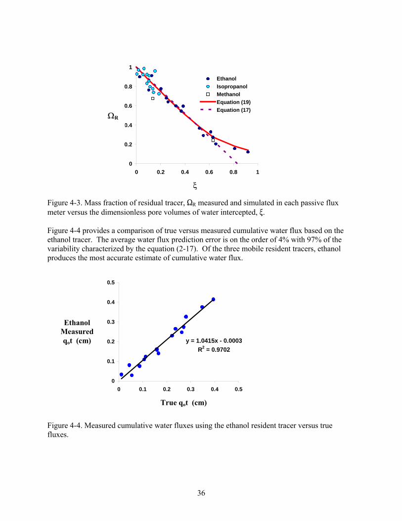
0

0.2

0.4

0.6

0.8

1

0 0.2 0.4 0.6 0.8 1

EthanolIsopropanolMethanolEquation (19)Equation (17)

ξ

ΩR

Figure 4-3. Mass fraction of residual tracer, SR measured and simulated in each passive flux meter versus the dimensionless pore volumes of water intercepted, >. Figure 4-4 provides a comparison of true versus measured cumulative water flux based on the ethanol tracer. The average water flux prediction error is on the order of 4% with 97% of the variability characterized by the equation (2-17). Of the three mobile resident tracers, ethanol produces the most accurate estimate of cumulative water flux.

y = 1.0415x - 0.0003R2 = 0.9702

0

0.1

0.2

0.3

0.4

0.5

0 0.1 0.2 0.3 0.4 0.5

True qot (cm)

Ethanol Measured qot (cm)

Figure 4-4. Measured cumulative water fluxes using the ethanol resident tracer versus true fluxes.

36

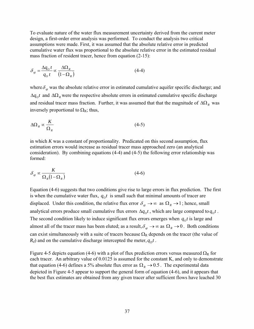
To evaluate nature of the water flux measurement uncertainty derived from the current meter design, a first-order error analysis was performed. To conduct the analysis two critical assumptions were made. First, it was assumed that the absolute relative error in predicted cumulative water flux was proportional to the absolute relative error in the estimated residual mass fraction of resident tracer, hence from equation (2-15):

( )R

R

O

Oqt tq

tqΩ−

∆Ω∝

∆=

1δ (4-4)

where qtδ was the absolute relative error in estimated cumulative aquifer specific discharge; and

and were the respective absolute errors in estimated cumulative specific discharge and residual tracer mass fraction. Further, it was assumed that that the magnitude of was inversely proportional to Ω

tqO∆ R∆Ω

R∆ΩR; thus,

RR

KΩ

∝∆Ω (4-5)

in which K was a constant of proportionality. Predicated on this second assumption, flux estimation errors would increase as residual tracer mass approached zero (an analytical consideration). By combining equations (4-4) and (4-5) the following error relationship was formed:

( )RRqt

KΩ−Ω

∝1

δ (4-6)

Equation (4-6) suggests that two conditions give rise to large errors in flux prediction. The first is when the cumulative water flux, is small such that minimal amounts of tracer are displaced. Under this condition, the relative flux error

tqO

∞→qtδ as 1→ΩR ; hence, small analytical errors produce small cumulative flux errors tqO∆ , which are large compared to . The second condition likely to induce significant flux errors emerges when is large and almost all of the tracer mass has been eluted; as a result,

tqO

tqO

∞→qtδ as 0→ΩR . Both conditions can exist simultaneously with a suite of tracers because ΩR depends on the tracer (the value of Rd) and on the cumulative discharge intercepted the meter, . tqD

Figure 4-5 depicts equation (4-6) with a plot of flux prediction errors versus measured ΩR for each tracer. An arbitrary value of 0.0125 is assumed for the constant K, and only to demonstrate that equation (4-6) defines a 5% absolute flux error as 5.0→ΩR . The experimental data depicted in Figure 4-5 appear to support the general form of equation (4-6), and it appears that the best flux estimates are obtained from any given tracer after sufficient flows have leached 30

37

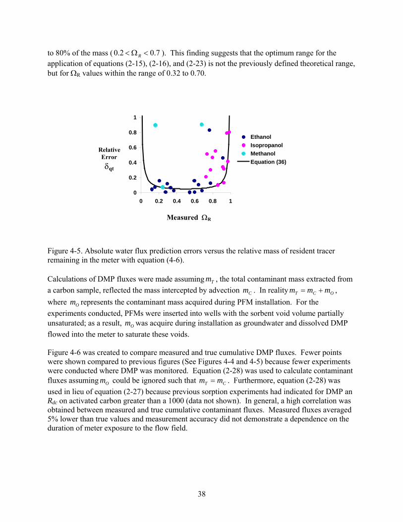
to 80% of the mass ( ). This finding suggests that the optimum range for the application of equations (2-15), (2-16), and (2-23) is not the previously defined theoretical range, but for Ω

7.02.0 <Ω< R

R values within the range of 0.32 to 0.70.

0

0.2

0.4

0.6

0.8

1

0 0.2 0.4 0.6 0.8 1

EthanolIsopropanolMethanolEquation (36)

Relative Error δqt

Measured ΩR

Figure 4-5. Absolute water flux prediction errors versus the relative mass of resident tracer remaining in the meter with equation (4-6). Calculations of DMP fluxes were made assuming , the total contaminant mass extracted from a carbon sample, reflected the mass intercepted by advection . In reality , where represents the contaminant mass acquired during PFM installation. For the experiments conducted, PFMs were inserted into wells with the sorbent void volume partially unsaturated; as a result, was acquire during installation as groundwater and dissolved DMP flowed into the meter to saturate these voids.

Tm

Cm OCT mmm +=

Om

Om

Figure 4-6 was created to compare measured and true cumulative DMP fluxes. Fewer points were shown compared to previous figures (See Figures 4-4 and 4-5) because fewer experiments were conducted where DMP was monitored. Equation (2-28) was used to calculate contaminant fluxes assuming could be ignored such that Om CT mm = . Furthermore, equation (2-28) was used in lieu of equation (2-27) because previous sorption experiments had indicated for DMP an Rdc on activated carbon greater than a 1000 (data not shown). In general, a high correlation was obtained between measured and true cumulative contaminant fluxes. Measured fluxes averaged 5% lower than true values and measurement accuracy did not demonstrate a dependence on the duration of meter exposure to the flow field.

38

y = 0.9485x + 0.0057R2 = 0.9673

0

1

2

3

4

0 1 2 3 4

True Jct (mg/cm2)

Measured Jct

(mg/cm2)

Figure 4-6. Measured cumulative DMP fluxes versus true fluxes. To evaluate the significance of ignoring , consideration must be given to volume of water intercepted by the meter under natural gradient conditions versus the volume taken up during meter installation. For example, if the cumulative volume of water intercepted is small, such that

Om

ξ is on the order of dcR1 , then equating and can lead to erroneous flux estimates because much of sorbed contaminant reflects and not . In general, with an increase in the volume of water intercepted, will increase and flux estimation errors will decrease to a value proportional to and the analytical limitations of the methods used for contaminant extraction/analysis. These observations are summarized in the following contaminant flux error equation (4-7).

Cm Tm

Om Cm

Cm

Cm

( ) ( )

FO

FFO

C

OC

OT

T

C

CJt trbcq

cbrtrbcqm

mmmm

mtJtJ

22 2 θπδ +∆

=+∆

=−

∆=

∆= (4-7)

where Jtδ is the absolute relative error in estimated cumulative contaminant flux; is the absolute error in the cumulative contaminant flux, [M]; and

tJT

∆Tm∆ is the absolute error in the total

contaminant mass extracted from a carbon sample, [M]. Equation (4-7) states that large relative errors in measured contaminant fluxes can be expected when small volumes of water are intercepted under low flow conditions or from brief sampling periods resulting in an ; however, from long-term monitoring giving rise to values of , it can be seen that

OT mm →

OT mm >>

CCJt mm∆→δ . This later finding assumes the application of equation (2-28) and all appurtenant restrictions coupled to that equation.

39

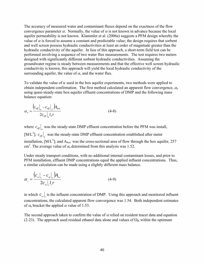
The accuracy of measured water and contaminant fluxes depend on the exactness of the flow convergence parameter α. Normally, the value of α is not known in advance because the local aquifer permeability is not known. Klammler et al. (2006a) suggests a PFM design whereby the value of α is forced to assume a constant and predictable value; the design requires that sorbent and well screen possess hydraulic conductivities at least an order of magnitude greater than the hydraulic conductivity of the aquifer. In lieu of this approach, a short-term field test can be performed involving a sequence of two water flux measurements. The test requires two meters designed with significantly different sorbent hydraulic conductivities. Assuming the groundwater regime is steady between measurements and that the effective well screen hydraulic conductivity is known, this approach will yield the local hydraulic conductivity of the surrounding aquifer, the value of α, and the water flux. To validate the value of α used in the box aquifer experiments, two methods were applied to obtain independent confirmation. The first method calculated an apparent flow convergence, αe using quasi-steady-state box-aquifer effluent concentrations of DMP and the following mass balance equation:

( )rlc

Acc

Soeff

boxfeffoeff

e 2

−=α (4-8)

where

oeffc was the steady-state DMP effluent concentration before the PFM was install,

[M/L3]; feffc was the steady-state DMP effluent concentration established after meter

installation, [M/L3]; and Abox was the cross-sectional area of flow through the box aquifer, 257 cm2. The average value of αe determined from this analysis was 1.52. Under steady transport conditions, with no additional internal contaminant losses, and prior to PFM installation, effluent DMP concentrations equal the applied influent concentrations. Thus, a similar calculation can be made using a slightly different mass balance.

( )rlc

Acc

So

boxfeffo

e

inf

inf

2−

=α (4-9)

in which

oc

infis the influent concentration of DMP. Using this approach and monitored influent

concentrations, the calculated apparent flow convergence was 1.54. Both independent estimates of αe bracket the applied α value of 1.53. The second approach taken to confirm the value of α relied on resident tracer data and equation (2-23). The approach used residual ethanol data alone and values of ΩR within the optimum

40

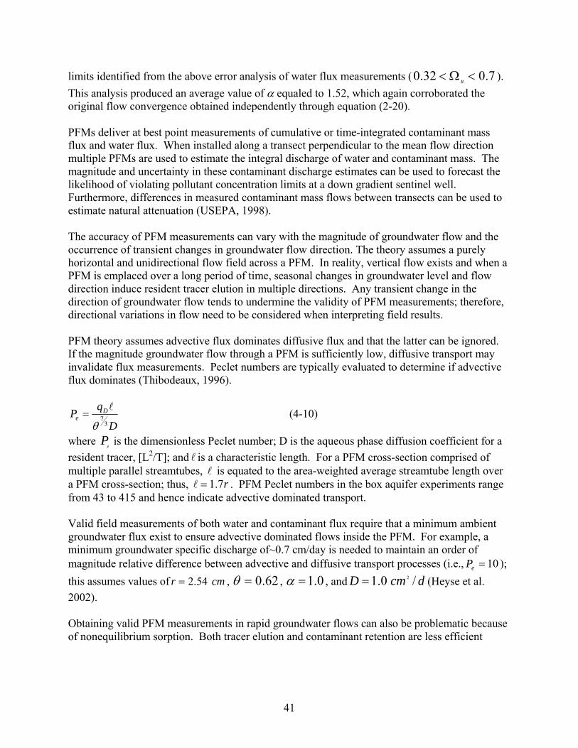
limits identified from the above error analysis of water flux measurements ( 7.032.0 <Ω<R

). This analysis produced an average value of α equaled to 1.52, which again corroborated the original flow convergence obtained independently through equation (2-20). PFMs deliver at best point measurements of cumulative or time-integrated contaminant mass flux and water flux. When installed along a transect perpendicular to the mean flow direction multiple PFMs are used to estimate the integral discharge of water and contaminant mass. The magnitude and uncertainty in these contaminant discharge estimates can be used to forecast the likelihood of violating pollutant concentration limits at a down gradient sentinel well. Furthermore, differences in measured contaminant mass flows between transects can be used to estimate natural attenuation (USEPA, 1998). The accuracy of PFM measurements can vary with the magnitude of groundwater flow and the occurrence of transient changes in groundwater flow direction. The theory assumes a purely horizontal and unidirectional flow field across a PFM. In reality, vertical flow exists and when a PFM is emplaced over a long period of time, seasonal changes in groundwater level and flow direction induce resident tracer elution in multiple directions. Any transient change in the direction of groundwater flow tends to undermine the validity of PFM measurements; therefore, directional variations in flow need to be considered when interpreting field results. PFM theory assumes advective flux dominates diffusive flux and that the latter can be ignored. If the magnitude groundwater flow through a PFM is sufficiently low, diffusive transport may invalidate flux measurements. Peclet numbers are typically evaluated to determine if advective flux dominates (Thibodeaux, 1996).

D

qP De

37

θ

l= (4-10)

where is the dimensionless Peclet number; D is the aqueous phase diffusion coefficient for a resident tracer, [L

eP

2/T]; and is a characteristic length. For a PFM cross-section comprised of multiple parallel streamtubes, is equated to the area-weighted average streamtube length over a PFM cross-section; thus, . PFM Peclet numbers in the box aquifer experiments range from 43 to 415 and hence indicate advective dominated transport.

ll

r7.1=l

Valid field measurements of both water and contaminant flux require that a minimum ambient groundwater flux exist to ensure advective dominated flows inside the PFM. For example, a minimum groundwater specific discharge of~0.7 cm/day is needed to maintain an order of magnitude relative difference between advective and diffusive transport processes (i.e., 10=eP ); this assumes values of , cmr 54.2= 62.0=θ , 0.1=α , and dcmD /0.1 2= (Heyse et al. 2002). Obtaining valid PFM measurements in rapid groundwater flows can also be problematic because of nonequilibrium sorption. Both tracer elution and contaminant retention are less efficient

41

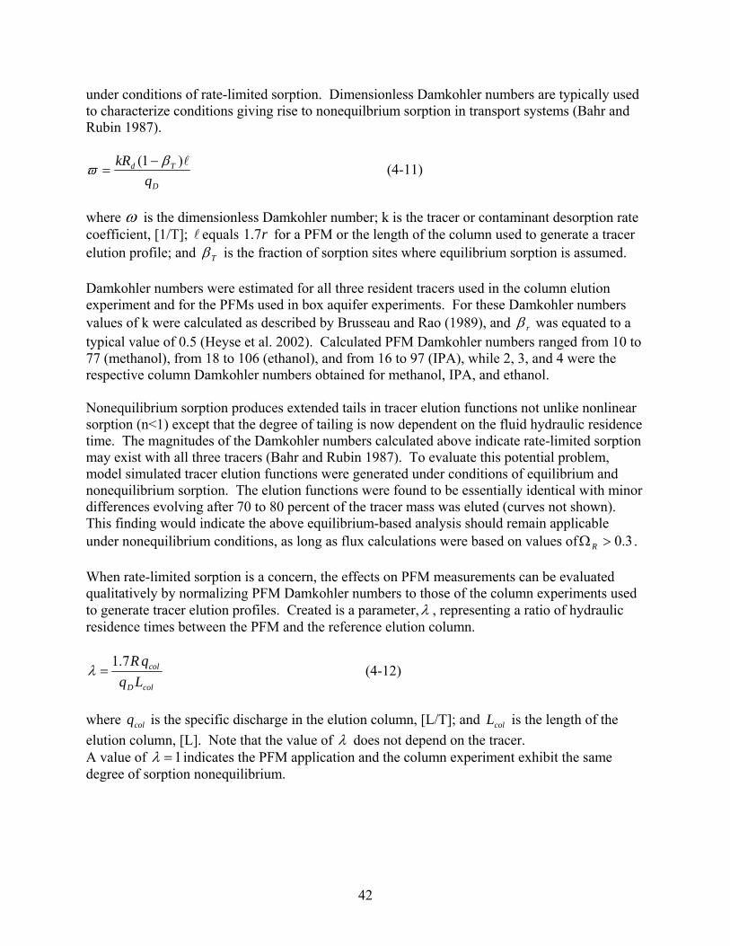
under conditions of rate-limited sorption. Dimensionless Damkohler numbers are typically used to characterize conditions giving rise to nonequilbrium sorption in transport systems (Bahr and Rubin 1987).

D

Td

qkR l)1( βϖ −

= (4-11)

where ω is the dimensionless Damkohler number; k is the tracer or contaminant desorption rate coefficient, [1/T]; equals for a PFM or the length of the column used to generate a tracer elution profile; and

l r7.1Tβ is the fraction of sorption sites where equilibrium sorption is assumed.

Damkohler numbers were estimated for all three resident tracers used in the column elution experiment and for the PFMs used in box aquifer experiments. For these Damkohler numbers values of k were calculated as described by Brusseau and Rao (1989), and rβ was equated to a typical value of 0.5 (Heyse et al. 2002). Calculated PFM Damkohler numbers ranged from 10 to 77 (methanol), from 18 to 106 (ethanol), and from 16 to 97 (IPA), while 2, 3, and 4 were the respective column Damkohler numbers obtained for methanol, IPA, and ethanol. Nonequilibrium sorption produces extended tails in tracer elution functions not unlike nonlinear sorption (n<1) except that the degree of tailing is now dependent on the fluid hydraulic residence time. The magnitudes of the Damkohler numbers calculated above indicate rate-limited sorption may exist with all three tracers (Bahr and Rubin 1987). To evaluate this potential problem, model simulated tracer elution functions were generated under conditions of equilibrium and nonequilibrium sorption. The elution functions were found to be essentially identical with minor differences evolving after 70 to 80 percent of the tracer mass was eluted (curves not shown). This finding would indicate the above equilibrium-based analysis should remain applicable under nonequilibrium conditions, as long as flux calculations were based on values of . 3.0>ΩR

When rate-limited sorption is a concern, the effects on PFM measurements can be evaluated qualitatively by normalizing PFM Damkohler numbers to those of the column experiments used to generate tracer elution profiles. Created is a parameter,λ , representing a ratio of hydraulic residence times between the PFM and the reference elution column.

colD

col

LqqR7.1

=λ (4-12)

where is the specific discharge in the elution column, [L/T]; and is the length of the elution column, [L]. Note that the value of

colq colLλ does not depend on the tracer.

A value of 1=λ indicates the PFM application and the column experiment exhibit the same degree of sorption nonequilibrium.

42

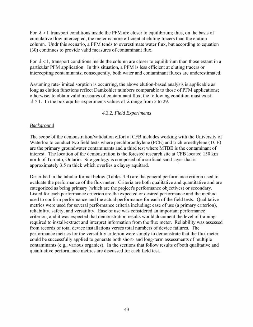
43

1>For λ transport conditions inside the PFM are closer to equilibrium; thus, on the basis of cumulative flow intercepted, the meter is more efficient at eluting tracers than the elution column. Undr this scenario, a PFM tends to overestimate water flux, but according to equation (30) continues to provide valid measures of contaminant flux. For 1<λ , transport conditions inside the column are closer to equilibrium than those extant in a particular PFM application. In this situation, a PFM is less efficient at eluting tracers or intercepting contaminants; consequently, both water and contaminant fluxes are underestimated. Assuming rate-limited sorption is occurring, the above elution-based analysis is applicable as long as elution functions reflect Damkohler numbers comparable to those of PFM applications; otherwise, to obtain valid measures of contaminant flux, the following condition must exist:

1≥λ . In the box aquifer experiments values of λ range from 5 to 29.

4.3.2. Field Experiments Background The scope of the demonstration/validation effort at CFB includes working with the University of Waterloo to conduct two field tests where perchloroethylene (PCE) and trichloroethylene (TCE) are the primary groundwater contaminants and a third test where MTBE is the contaminant of interest. The location of the demonstration is the forested research site at CFB located 150 km north of Toronto, Ontario. Site geology is composed of a surficial sand layer that is approximately 3.5 m thick which overlies a clayey aquitard. Described in the tabular format below (Tables 4-4) are the general performance criteria used to evaluate the performance of the flux meter. Criteria are both qualitative and quantitative and are categorized as being primary (which are the project's performance objectives) or secondary. Listed for each performance criterion are the expected or desired performance and the method used to confirm performance and the actual performance for each of the field tests. Qualitative metrics were used for several performance criteria including: ease of use (a primary criterion), reliability, safety, and versatility. Ease of use was considered an important performance criterion, and it was expected that demonstration results would document the level of training required to install/extract and interpret information from the flux meter. Reliability was assessed from records of total device installations verses total numbers of device failures. The performance metrics for the versatility criterion were simply to demonstrate that the flux meter could be successfully applied to generate both short- and long-term assessments of multiple contaminants (e.g., various organics). In the sections that follow results of both qualitative and quantitative performance metrics are discussed for each field test.

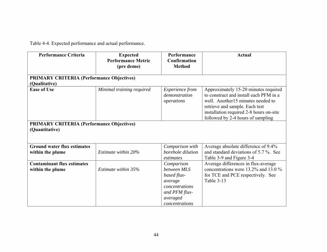
Table 4-4. Expected performance and actual performance.

Performance Criteria

Expected Performance Metric

(pre demo)

Performance Confirmation

Method

Actual

PRIMARY CRITERIA (Performance Objectives) (Qualitative) Ease of Use Minimal training required Experience from

demonstration operations

Approximately 15-20 minutes required to construct and install each PFM in a well. Another15 minutes needed to retrieve and sample. Each test installation required 2-8 hours on-site followed by 2-4 hours of sampling

PRIMARY CRITERIA (Performance Objectives) (Quantitative)

Ground water flux estimates within the plume

Estimate within 20%

Comparison with borehole dilution estimates

Average absolute difference of 9.4% and standard deviations of 5.7 %. See Table 3-9 and Figure 3-4

Contaminant flux estimates within the plume

Estimate within 35%

Comparison between MLS based flux-average concentrations and PFM flux-averaged concentrations

Average differences in flux-average concentrations were 13.2% and 13.0 % for TCE and PCE respectively. See Table 3-13

44

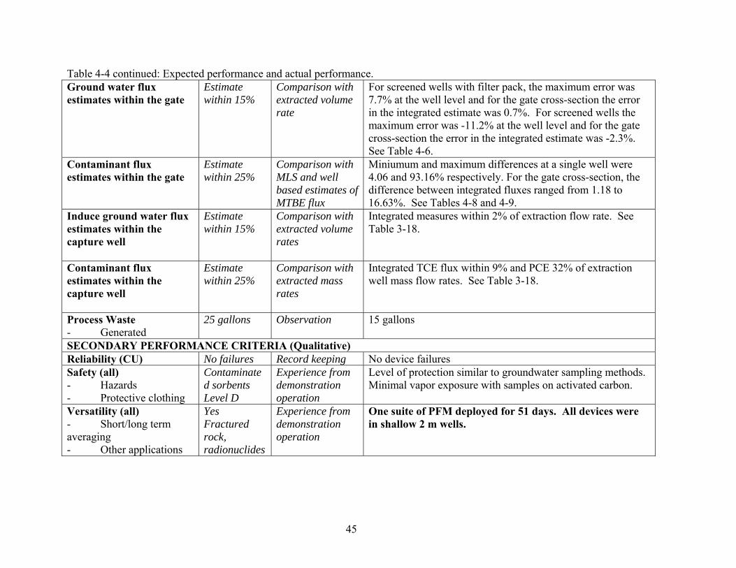
Table 4-4 continued: Expected performance and actual performance. Ground water flux estimates within the gate

Estimate within 15%

Comparison with extracted volume rate

For screened wells with filter pack, the maximum error was 7.7% at the well level and for the gate cross-section the error in the integrated estimate was 0.7%. For screened wells the maximum error was -11.2% at the well level and for the gate cross-section the error in the integrated estimate was -2.3%. See Table 4-6.

Contaminant flux estimates within the gate

Estimate within 25%

Comparison with MLS and well based estimates of MTBE flux

Miniumum and maximum differences at a single well were 4.06 and 93.16% respectively. For the gate cross-section, the difference between integrated fluxes ranged from 1.18 to 16.63%. See Tables 4-8 and 4-9.

Induce ground water flux estimates within the capture well

Estimate within 15%

Comparison with extracted volume rates

Integrated measures within 2% of extraction flow rate. See Table 3-18.

Contaminant flux estimates within the capture well

Estimate within 25%

Comparison with extracted mass rates

Integrated TCE flux within 9% and PCE 32% of extraction well mass flow rates. See Table 3-18.

Process Waste - Generated

25 gallons Observation 15 gallons

SECONDARY PERFORMANCE CRITERIA (Qualitative) Reliability (CU) No failures Record keeping No device failures Safety (all) - Hazards - Protective clothing

Contaminated sorbents Level D


Level of protection similar to groundwater sampling methods. Minimal vapor exposure with samples on activated carbon.

Versatility (all) - Short/long term averaging - Other applications

Yes Fractured rock, radionuclides


One suite of PFM deployed for 51 days. All devices were in shallow 2 m wells.

45

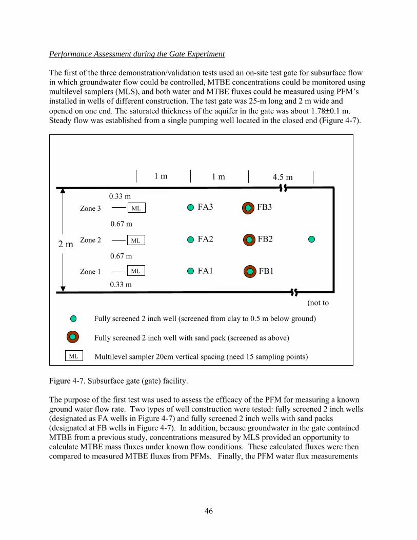
Performance Assessment during the Gate Experiment The first of the three demonstration/validation tests used an on-site test gate for subsurface flow in which groundwater flow could be controlled, MTBE concentrations could be monitored using multilevel samplers (MLS), and both water and MTBE fluxes could be measured using PFM’s installed in wells of different construction. The test gate was 25-m long and 2 m wide and opened on one end. The saturated thickness of the aquifer in the gate was about 1.78±0.1 m. Steady flow was established from a single pumping well located in the closed end (Figure 4-7).

ML

Fully screened 2 inch well (screened from clay to 0.5 m below ground)

Fully screened 2 inch well with sand pack (screened as above)

ML

ML

ML Multilevel sampler 20cm vertical spacing (need 15 sampling points)

2 m

0.67 m

0.33 m

0.33 m

0.67 m

1 m 1 m 4.5 m

(not to

FA1

FB3

FA2

FA3

FB2

FB1Zone 1

Zone 2

Zone 3

Figure 4-7. Subsurface gate (gate) facility. The purpose of the first test was used to assess the efficacy of the PFM for measuring a known ground water flow rate. Two types of well construction were tested: fully screened 2 inch wells (designated as FA wells in Figure 4-7) and fully screened 2 inch wells with sand packs (designated at FB wells in Figure 4-7). In addition, because groundwater in the gate contained MTBE from a previous study, concentrations measured by MLS provided an opportunity to calculate MTBE mass fluxes under known flow conditions. These calculated fluxes were then compared to measured MTBE fluxes from PFMs. Finally, the PFM water flux measurements

46

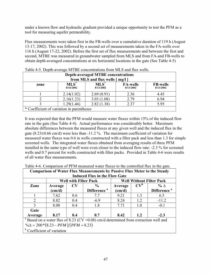
under a known flow and hydraulic gradient provided a unique opportunity to test the PFM as a tool for measuring aquifer permeability. Flux measurements were taken first in the FB-wells over a cumulative duration of 119 h (August 13-17, 2002). This was followed by a second set of measurements taken in the FA-wells over 116 h (August 17-22, 2002). Before the first set of flux measurements and between the first and second, MTBE was measured in groundwater sampled from MLS and from FA-and FB-wells to obtain depth-averaged concentrations at six horizontal locations in the gate (See Table 4-5)

Table 4-5. Depth-average MTBE concentrations from MLS and flux wells. Depth-averaged MTBE concentrations

from MLS and flux wells [ mg/l ] zone MLS*

8/16/2002MLS*

8/13/2002FA-wells

8/13/2002FB-wells

8/13/2002

1 2.14(1.02) 2.69 (0.91) 2.36 4.45 2 2.16(1.23) 3.03 (1.08) 2.79 6.94 3 1.29(1.46) 2.82 (1.38) 2.37 5.95

* Coefficient of variation in parentheses It was expected that that the PFM would measure water fluxes within 15% of the induced flow rate in the gate (See Table 4-4). Actual performance was considerably better. Maximum absolute differences between the measured fluxes at any given well and the induced flux in the gate (8.23±0.66 cm/d) were less than -11.2 %. The maximum coefficient of variation for measured water fluxes was 0.6 in wells constructed with a filter pack and less than 1.3 for simple screened wells. The integrated water fluxes obtained from averaging results of three PFM installed in the same type of well were even closer to the induced flow rate: -2.3 % for screened wells and 0.7 percent for wells constructed with filter packs. Provided in Table 4-6 were results of all water flux measurements.

Table 4-6. Comparison of PFM measured water fluxes to the controlled flux in the gate. Comparison of Water Flux Measurements by Passive Flux Meter to the Steady

Induced Flux in the Flow Gate Well with Filter Pack Well Without Filter Pack

Zone Average (cm/d)

CV

% Difference a

Average (cm/d)

CVb

% ∆

Difference a

1 7.62 0.6 7.7 9.21 1.3 6.5 2 8.82 0.4 -6.9 8.24 1.2 -11.2 3 8.08 0.4 1.8 7.71 1.0 -0.1

Gate Average 8.17 0.4 0.7 8.42 1.2 -2.3

a Based on a water flux of 8.23 (CV =0.08) cm/d determined from extraction well and ( ) ( )23.823.8*200% +−=∆ PFMPFM

b Coefficient of variation

47

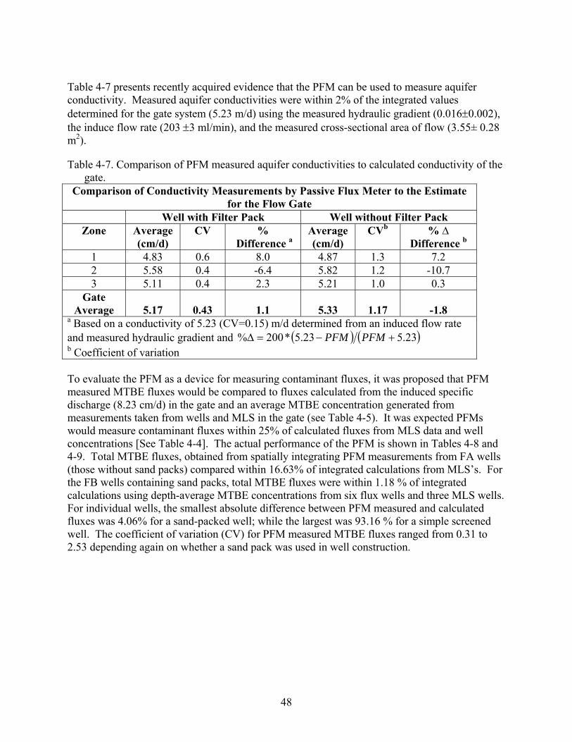
Table 4-7 presents recently acquired evidence that the PFM can be used to measure aquifer conductivity. Measured aquifer conductivities were within 2% of the integrated values determined for the gate system (5.23 m/d) using the measured hydraulic gradient (0.016±0.002), the induce flow rate (203 ±3 ml/min), and the measured cross-sectional area of flow (3.55± 0.28 m2).

Table 4-7. Comparison of PFM measured aquifer conductivities to calculated conductivity of the gate.

Comparison of Conductivity Measurements by Passive Flux Meter to the Estimate for the Flow Gate

Well with Filter Pack Well without Filter Pack Zone Average

(cm/d) CV

%

Difference aAverage (cm/d)

CVb

% ∆

Difference b

1 4.83 0.6 8.0 4.87 1.3 7.2 2 5.58 0.4 -6.4 5.82 1.2 -10.7 3 5.11 0.4 2.3 5.21 1.0 0.3

Gate Average 5.17 0.43 1.1 5.33 1.17 -1.8

a Based on a conductivity of 5.23 (CV=0.15) m/d determined from an induced flow rate and measured hydraulic gradient and ( ) ( )23.523.5*200% +−=∆ PFMPFM b Coefficient of variation To evaluate the PFM as a device for measuring contaminant fluxes, it was proposed that PFM measured MTBE fluxes would be compared to fluxes calculated from the induced specific discharge (8.23 cm/d) in the gate and an average MTBE concentration generated from measurements taken from wells and MLS in the gate (see Table 4-5). It was expected PFMs would measure contaminant fluxes within 25% of calculated fluxes from MLS data and well concentrations [See Table 4-4]. The actual performance of the PFM is shown in Tables 4-8 and 4-9. Total MTBE fluxes, obtained from spatially integrating PFM measurements from FA wells (those without sand packs) compared within 16.63% of integrated calculations from MLS’s. For the FB wells containing sand packs, total MTBE fluxes were within 1.18 % of integrated calculations using depth-average MTBE concentrations from six flux wells and three MLS wells. For individual wells, the smallest absolute difference between PFM measured and calculated fluxes was 4.06% for a sand-packed well; while the largest was 93.16 % for a simple screened well. The coefficient of variation (CV) for PFM measured MTBE fluxes ranged from 0.31 to 2.53 depending again on whether a sand pack was used in well construction.

48

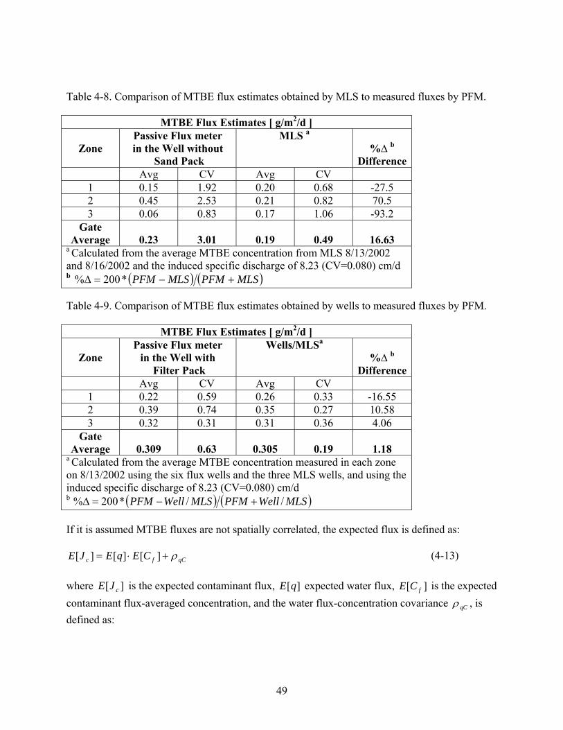
Table 4-8. Comparison of MTBE flux estimates obtained by MLS to measured fluxes by PFM.

MTBE Flux Estimates [ g/m2/d ]

Zone Passive Flux meter in the Well without

Sand Pack

MLS a %∆ b

Difference Avg CV Avg CV 1 0.15 1.92 0.20 0.68 -27.5 2 0.45 2.53 0.21 0.82 70.5 3 0.06 0.83 0.17 1.06 -93.2

Gate Average 0.23 3.01 0.19 0.49 16.63

a Calculated from the average MTBE concentration from MLS 8/13/2002 and 8/16/2002 and the induced specific discharge of 8.23 (CV=0.080) cm/d b ( ) ( )MLSPFMMLSPFM +−=∆ *200%

Table 4-9. Comparison of MTBE flux estimates obtained by wells to measured fluxes by PFM.

MTBE Flux Estimates [ g/m2/d ]

Zone Passive Flux meter

in the Well with Filter Pack

Wells/MLSa %∆ b

Difference Avg CV Avg CV 1 0.22 0.59 0.26 0.33 -16.55 2 0.39 0.74 0.35 0.27 10.58 3 0.32 0.31 0.31 0.36 4.06

Gate Average 0.309 0.63 0.305 0.19 1.18

a Calculated from the average MTBE concentration measured in each zone on 8/13/2002 using the six flux wells and the three MLS wells, and using the induced specific discharge of 8.23 (CV=0.080) cm/d b ( ) ( )MLSWellPFMMLSWellPFM //*200% +−=∆ If it is assumed MTBE fluxes are not spatially correlated, the expected flux is defined as:

qCfc CEqEJE ρ+⋅= ][][][ (4-13) where is the expected contaminant flux, expected water flux, is the expected contaminant flux-averaged concentration, and the water flux-concentration covariance

][ cJE ][qE ][ fCE

qCρ , is defined as:

49

])][(])[[( ffqC CECqEqE −⋅−=ρ (4-14)

The PFM measures water flux directly and the contaminant mass intercepted and retained on the device can be used to calculate local flux-averaged contaminant concentrations. From Table 4-10, the covariance is shown to be relatively large (~19-48%) with respect to the expected mass flux. Thus, for the gate experiments, water flux and MTBE concentrations are strongly correlated; consequently, the expected flux cannot be approximated as simply the product of the mean water flux and the mean flux-averaged concentration derived from PFM measurements.

][][][ fc CEqEJE ⋅≅ (4-15)

Table 4-10. Comparisons of the expected value of MTBE flux, to the flux calculated from taking the product of the expected values for water flux and MTBE flux-averaged concentration, and the covariance between water flux and MTBE flux-averaged concentration.

PFM Derived Expected MTBE Flux and Covariance ][JE qCρ Between Water Flux and Flux-averaged Concentration

Calculated Fluxa,d

g/m2/d

Water-Contaminant Covarianceb

g/m2/d

Expected Fluxc

g/m2/d

Relative weight of the

covariance

Well Type

][][ fCEqE ∗ qCρ ][JE 100* ][/ JEqCρ

Simple Screen 0.12 (0.67)

0.11

0.23

48.0

Screen with Filter pack

0.37 (-0.53)

-0.06

0.31

19.0

a from the product of the expected water flux and MTBE flux-averaged ][qE concentration ][ fCEb covariance between water flux and flux-averaged concentration c from averaging PFM measurements over gate cross-section d correlation between and in parentheses q fC

50

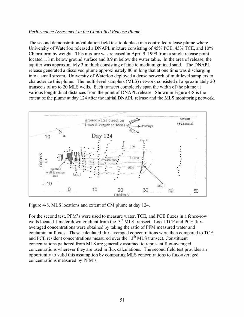
Performance Assessment in the Controlled Release Plume The second demonstration/validation field test took place in a controlled release plume where University of Waterloo released a DNAPL mixture consisting of 45% PCE, 45% TCE, and 10% Chloroform by weight. This mixture was released in April 9, 1999 from a single release point located 1.8 m below ground surface and 0.9 m below the water table. In the area of release, the aquifer was approximately 3 m thick consisting of fine to medium grained sand. The DNAPL release generated a dissolved plume approximately 80 m long that at one time was discharging into a small stream. University of Waterloo deployed a dense network of multilevel samplers to characterize this plume. The multi-level samplers (MLS) network consisted of approximately 20 transects of up to 20 MLS wells. Each transect completely span the width of the plume at various longitudinal distances from the point of DNAPL release. Shown in Figure 4-8 is the extent of the plume at day 124 after the initial DNAPL release and the MLS monitoring network.

Figure 4-8. MLS locations and extent of CM plume at day 124. For the second test, PFM’s were used to measure water, TCE, and PCE fluxes in a fence-row wells located 1 meter down gradient from the13th MLS transect. Local TCE and PCE flux-averaged concentrations were obtained by taking the ratio of PFM measured water and contaminant fluxes. These calculated flux-averaged concentrations were then compared to TCE and PCE resident concentrations measured over the 13th MLS transect. Constituent concentrations gathered from MLS are generally assumed to represent flux-averaged concentrations wherever they are used in flux calculations. The second field test provides an opportunity to valid this assumption by comparing MLS concentrations to flux-averaged concentrations measured by PFM’s.

51

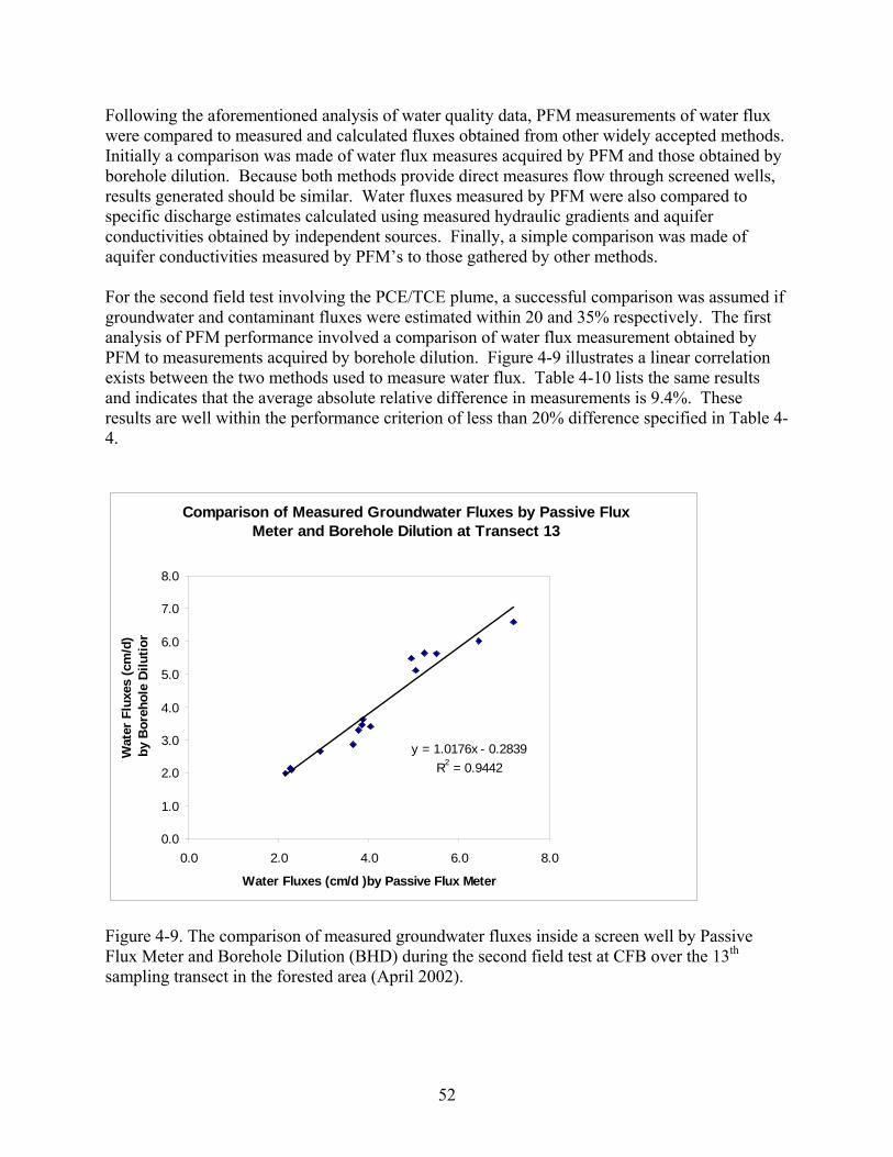
Following the aforementioned analysis of water quality data, PFM measurements of water flux were compared to measured and calculated fluxes obtained from other widely accepted methods. Initially a comparison was made of water flux measures acquired by PFM and those obtained by borehole dilution. Because both methods provide direct measures flow through screened wells, results generated should be similar. Water fluxes measured by PFM were also compared to specific discharge estimates calculated using measured hydraulic gradients and aquifer conductivities obtained by independent sources. Finally, a simple comparison was made of aquifer conductivities measured by PFM’s to those gathered by other methods. For the second field test involving the PCE/TCE plume, a successful comparison was assumed if groundwater and contaminant fluxes were estimated within 20 and 35% respectively. The first analysis of PFM performance involved a comparison of water flux measurement obtained by PFM to measurements acquired by borehole dilution. Figure 4-9 illustrates a linear correlation exists between the two methods used to measure water flux. Table 4-10 lists the same results and indicates that the average absolute relative difference in measurements is 9.4%. These results are well within the performance criterion of less than 20% difference specified in Table 4-4.

Comparison of Measured Groundwater Fluxes by Passive Flux Meter and Borehole Dilution at Transect 13

y = 1.0176x - 0.2839R2 = 0.9442

0.0

1.0

2.0

3.0

4.0

5.0

6.0

7.0

8.0

0.0 2.0 4.0 6.0 8.0

Water Fluxes (cm/d )by Passive Flux Meter

Wat

er F

luxe

s (c

m/d

) b

y B

oreh

ole

Dilu

tion

Figure 4-9. The comparison of measured groundwater fluxes inside a screen well by Passive Flux Meter and Borehole Dilution (BHD) during the second field test at CFB over the 13th sampling transect in the forested area (April 2002).

52

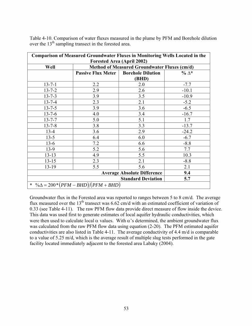
Table 4-10. Comparison of water fluxes measured in the plume by PFM and Borehole dilution over the 13th sampling transect in the forested area. Comparison of Measured Groundwater Fluxes in Monitoring Wells Located in the

Forested Area (April 2002) Well Method of Measured Groundwater Fluxes (cm/d)

Passive Flux Meter Borehole Dilution (BHD)

% ∆*

13-7-1 2.2 2.0 -7.7 13-7-2 2.9 2.6 -10.1 13-7-3 3.9 3.5 -10.9 13-7-4 2.3 2.1 -5.2 13-7-5 3.9 3.6 -6.5 13-7-6 4.0 3.4 -16.7 13-7-7 5.0 5.1 1.7 13-7-8 3.8 3.3 -13.7 13-4 3.6 2.9 -24.2 13-5 6.4 6.0 -6.7 13-6 7.2 6.6 -8.8 13-9 5.2 5.6 7.7 13-13 4.9 5.5 10.3 13-15 2.3 2.1 -8.8 13-19 5.5 5.6 2.1

Average Absolute Difference 9.4 Standard Deviation 5.7

* ( ) ( )BHDPFMBHDPFM +−=∆ *200% Groundwater flux in the Forested area was reported to ranges between 5 to 8 cm/d. The average flux measured over the 13th transect was 6.62 cm/d with an estimated coefficient of variation of 0.33 (see Table 4-11). The raw PFM flow data provide direct measure of flow inside the device. This data was used first to generate estimates of local aquifer hydraulic conductivities, which were then used to calculate local α values. With α’s determined, the ambient groundwater flux was calculated from the raw PFM flow data using equation (2-20). The PFM estimated aquifer conductivities are also listed in Table 4-11. The average conductivity of 4.4 m/d is comparable to a value of 5.25 m/d, which is the average result of multiple slug tests performed in the gate facility located immediately adjacent to the forested area Labaky (2004).

53

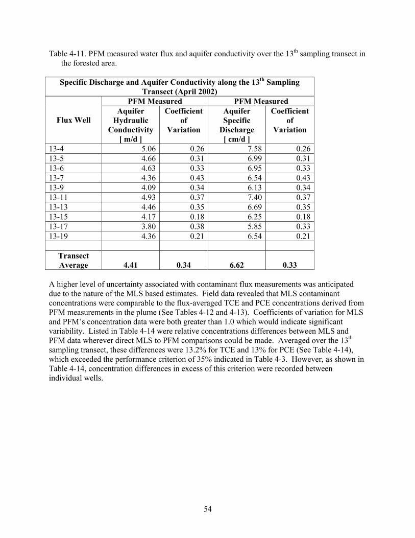
Table 4-11. PFM measured water flux and aquifer conductivity over the 13th sampling transect in the forested area.

Specific Discharge and Aquifer Conductivity along the 13th Sampling

Transect (April 2002) PFM Measured PFM Measured

Flux Well

Aquifer Hydraulic

Conductivity [ m/d ]

Coefficient of

Variation

Aquifer Specific

Discharge [ cm/d ]

Coefficient of

Variation

13-4 5.06 0.26 7.58 0.26 13-5 4.66 0.31 6.99 0.31 13-6 4.63 0.33 6.95 0.33 13-7 4.36 0.43 6.54 0.43 13-9 4.09 0.34 6.13 0.34 13-11 4.93 0.37 7.40 0.37 13-13 4.46 0.35 6.69 0.35 13-15 4.17 0.18 6.25 0.18 13-17 3.80 0.38 5.85 0.33 13-19 4.36 0.21 6.54 0.21

Transect Average

4.41

0.34

6.62

0.33

A higher level of uncertainty associated with contaminant flux measurements was anticipated due to the nature of the MLS based estimates. Field data revealed that MLS contaminant concentrations were comparable to the flux-averaged TCE and PCE concentrations derived from PFM measurements in the plume (See Tables 4-12 and 4-13). Coefficients of variation for MLS and PFM’s concentration data were both greater than 1.0 which would indicate significant variability. Listed in Table 4-14 were relative concentrations differences between MLS and PFM data wherever direct MLS to PFM comparisons could be made. Averaged over the 13th sampling transect, these differences were 13.2% for TCE and 13% for PCE (See Table 4-14), which exceeded the performance criterion of 35% indicated in Table 4-3. However, as shown in Table 4-14, concentration differences in excess of this criterion were recorded between individual wells.

54

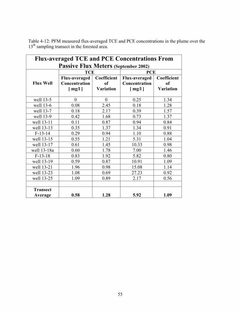
Table 4-12: PFM measured flux-averaged TCE and PCE concentrations in the plume over the 13th sampling transect in the forested area.

Flux-averaged TCE and PCE Concentrations From Passive Flux Meters (September 2002)

TCE PCE

Flux Well Flux-averaged Concentration

[ mg/l ]

Coefficient of

Variation

Flux-averagedConcentration

[ mg/l ]

Coefficient of

Variation

well 13-5 0 0 0.25 1.34 well 13-6 0.08 2.45 0.18 1.28 well 13-7 0.18 2.17 0.39 1.57 well 13-9 0.42 1.68 0.73 1.37 well 13-11 0.11 0.87 0.94 0.84 well 13-13 0.35 1.37 1.34 0.91

F-13-14 0.29 0.94 1.10 0.88 well 13-15 0.55 1.21 5.31 1.04 well 13-17 0.61 1.45 10.33 0.98 well 13-18a 0.60 1.78 7.00 1.46

F-13-18 0.83 1.92 5.82 0.80 well 13-19 0.59 0.87 10.91 1.09 well 13-21 1.96 0.98 15.08 1.14 well 13-23 1.08 0.69 27.23 0.92 well 13-25 1.09 0.89 2.17 0.56

Transect Average 0.58 1.28 5.92 1.09

55

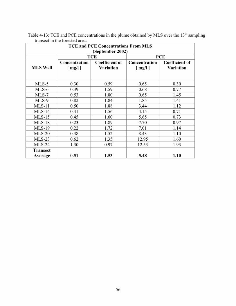
Table 4-13: TCE and PCE concentrations in the plume obtained by MLS over the 13th sampling transect in the forested area.

TCE and PCE Concentrations From MLS (September 2002)

TCE PCE

MLS Well Concentration

[ mg/l ] Coefficient of

Variation Concentration

[ mg/l ] Coefficient of

Variation

MLS-5 0.30 0.59 0.65 0.30 MLS-6 0.39 1.59 0.68 0.77 MLS-7 0.53 1.80 0.65 1.45 MLS-9 0.82 1.84 1.85 1.41 MLS-11 0.50 1.88 3.44 1.12 MLS-14 0.41 1.56 4.15 0.71 MLS-15 0.45 1.60 5.65 0.73 MLS-18 0.23 1.89 7.70 0.97 MLS-19 0.22 1.72 7.01 1.14 MLS-20 0.38 1.52 8.43 1.10 MLS-23 0.62 1.35 12.95 1.60 MLS-24 1.30 0.97 12.53 1.93 Transect Average 0.51 1.53 5.48 1.10

56

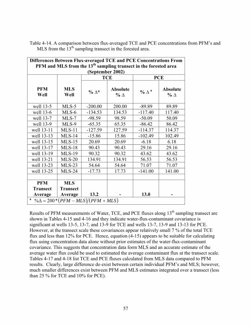
Table 4-14. A comparison between flux-averaged TCE and PCE concentrations from PFM’s and MLS from the 13th sampling transect in the forested area.

Differences Between Flux-averaged TCE and PCE Concentrations From

PFM and MLS from the 13th sampling transect in the forested area (September 2002)

TCE PCE

PFM Well

MLS Well % ∆* Absolute

% ∆ % ∆ a Absolute % ∆

well 13-5 MLS-5 -200.00 200.00 -89.89 89.89 well 13-6 MLS-6 -134.53 134.53 -117.40 117.40 well 13-7 MLS-7 -98.59 98.59 -50.09 50.09 well 13-9 MLS-9 -65.35 65.35 -86.42 86.42 well 13-11 MLS-11 -127.59 127.59 -114.37 114.37 well 13-13 MLS-14 -15.86 15.86 -102.49 102.49 well 13-15 MLS-15 20.69 20.69 -6.18 6.18 well 13-17 MLS-18 90.43 90.43 29.16 29.16 well 13-19 MLS-19 90.32 90.32 43.62 43.62 well 13-21 MLS-20 134.91 134.91 56.53 56.53 well 13-23 MLS-23 54.64 54.64 71.07 71.07 well 13-25 MLS-24 -17.73 17.73 -141.00 141.00

PFM

Transect Average

MLS Transect Average 13.2 - 13.0 -

a ( ) ( )MLSPFMMLSPFM +−=∆ *200% Results of PFM measurements of Water, TCE, and PCE fluxes along 13th sampling transect are shown in Tables 4-15 and 4-16 and they indicate water-flux-contaminant covariance is significant at wells 13-5, 13-7, and 13-9 for TCE and wells 13-7, 13-9 and 13-13 for PCE. However, at the transect scale these covariances appear relatively small 7 % of the total TCE flux and less than 12% for PCE. Hence, equation (4-15) appears to be suitable for calculating flux using concentration data alone without prior estimates of the water-flux-contaminant covariance. This suggests that concentration data form MLS and an accurate estimate of the average water flux could be used to estimated the average contaminant flux at the transect scale. Tables 4-17 and 4-18 list TCE and PCE fluxes calculated from MLS data compared to PFM results. Clearly, large difference do exist between certain individual PFM’s and MLS; however, much smaller differences exist between PFM and MLS estimates integrated over a transect (less than 25 % for TCE and 10% for PCE).

57

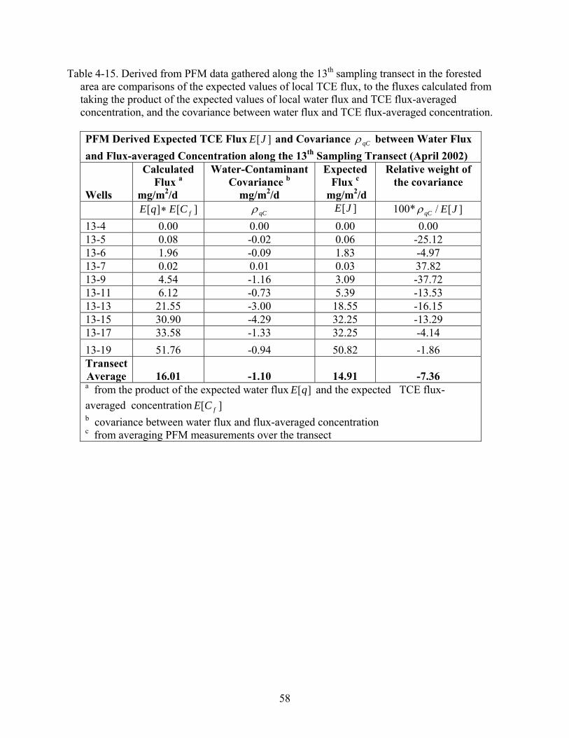
Table 4-15. Derived from PFM data gathered along the 13th sampling transect in the forested area are comparisons of the expected values of local TCE flux, to the fluxes calculated from taking the product of the expected values of local water flux and TCE flux-averaged concentration, and the covariance between water flux and TCE flux-averaged concentration.

PFM Derived Expected TCE Flux and Covariance ][JE qCρ between Water Flux and Flux-averaged Concentration along the 13th Sampling Transect (April 2002) Wells

Calculated Flux a

mg/m2/d

Water-Contaminant Covariance b

mg/m2/d

Expected Flux c

mg/m2/d

Relative weight of the covariance

][][ fCEqE ∗ qCρ ][JE 100* ][/ JEqCρ 13-4 0.00 0.00 0.00 0.00 13-5 0.08 -0.02 0.06 -25.12 13-6 1.96 -0.09 1.83 -4.97 13-7 0.02 0.01 0.03 37.82 13-9 4.54 -1.16 3.09 -37.72 13-11 6.12 -0.73 5.39 -13.53 13-13 21.55 -3.00 18.55 -16.15 13-15 30.90 -4.29 32.25 -13.29 13-17 33.58 -1.33 32.25 -4.14 13-19 51.76 -0.94 50.82 -1.86 Transect Average 16.01 -1.10 14.91 -7.36 a from the product of the expected water flux and the expected TCE flux-averaged concentration

][qE][ fCE

b covariance between water flux and flux-averaged concentration c from averaging PFM measurements over the transect

58

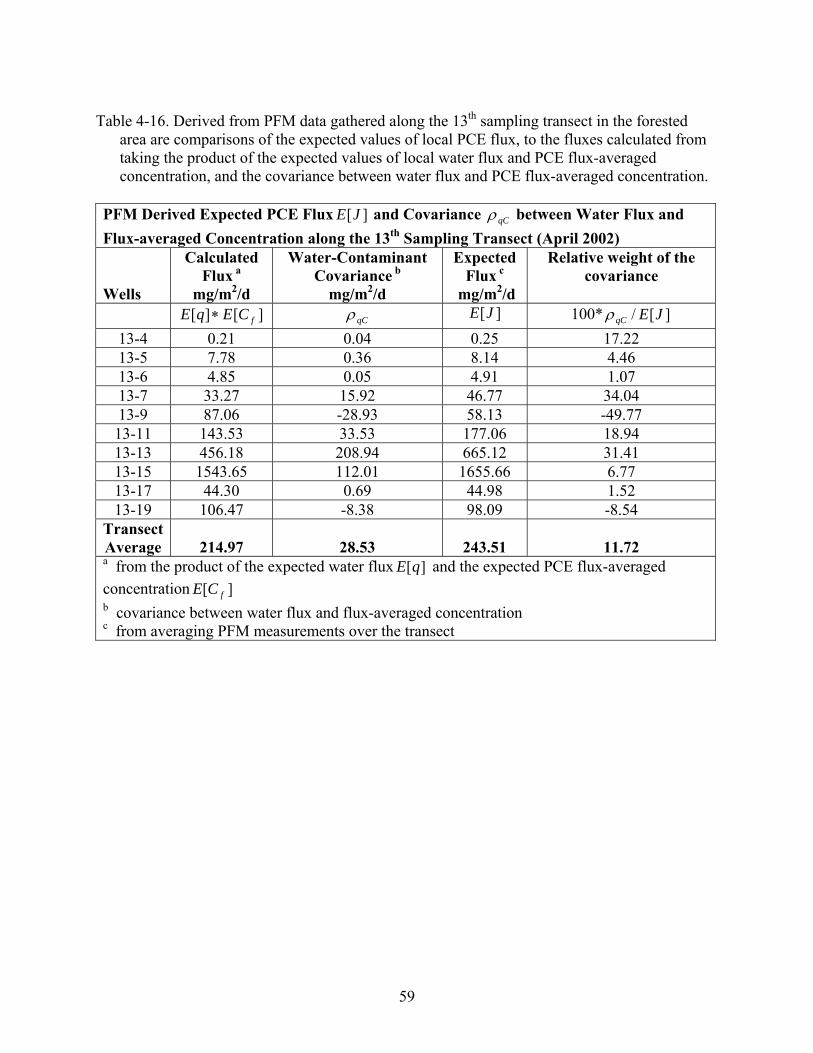
Table 4-16. Derived from PFM data gathered along the 13th sampling transect in the forested area are comparisons of the expected values of local PCE flux, to the fluxes calculated from taking the product of the expected values of local water flux and PCE flux-averaged concentration, and the covariance between water flux and PCE flux-averaged concentration.

PFM Derived Expected PCE Flux and Covariance ][JE qCρ between Water Flux and Flux-averaged Concentration along the 13th Sampling Transect (April 2002) Wells

Calculated Flux a

mg/m2/d

Water-Contaminant Covariance b

mg/m2/d

Expected Flux c

mg/m2/d

Relative weight of the covariance

][][ fCEqE ∗ qCρ ][JE 100* ][/ JEqCρ 13-4 0.21 0.04 0.25 17.22 13-5 7.78 0.36 8.14 4.46 13-6 4.85 0.05 4.91 1.07 13-7 33.27 15.92 46.77 34.04 13-9 87.06 -28.93 58.13 -49.77 13-11 143.53 33.53 177.06 18.94 13-13 456.18 208.94 665.12 31.41 13-15 1543.65 112.01 1655.66 6.77 13-17 44.30 0.69 44.98 1.52 13-19 106.47 -8.38 98.09 -8.54

Transect Average 214.97 28.53 243.51 11.72 a from the product of the expected water flux and the expected PCE flux-averaged concentration

][qE][ fCE

b covariance between water flux and flux-averaged concentration c from averaging PFM measurements over the transect

59

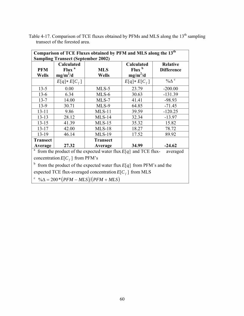
Table 4-17. Comparison of TCE fluxes obtained by PFMs and MLS along the 13th sampling transect of the forested area.

Comparison of TCE Fluxes obtained by PFM and MLS along the 13th Sampling Transect (September 2002)

PFM Wells

Calculated Flux a

mg/m2/d

MLS Wells

Calculated Flux b

mg/m2/d

Relative Difference

][][ fCEqE ∗ ][][ fCEqE ∗ %∆ c

13-5 0.00 MLS-5 23.79 -200.00 13-6 6.34 MLS-6 30.63 -131.39 13-7 14.00 MLS-7 41.41 -98.93 13-9 30.71 MLS-9 64.85 -71.45 13-11 9.86 MLS-11 39.59 -120.25 13-13 28.12 MLS-14 32.34 -13.97 13-15 41.39 MLS-15 35.32 15.82 13-17 42.00 MLS-18 18.27 78.72 13-19 46.14 MLS-19 17.52 89.92

Transect Average 27.32

Transect Average 34.99 -24.62

a from the product of the expected water flux and TCE flux- averaged concentration from PFM’s

][qE

)

][ fCEb from the product of the expected water flux from PFM’s and the expected TCE flux-averaged concentration from MLS

][qE][ fCE

c ( ) ( MLSPFMMLSPFM +−=∆ *200%

60

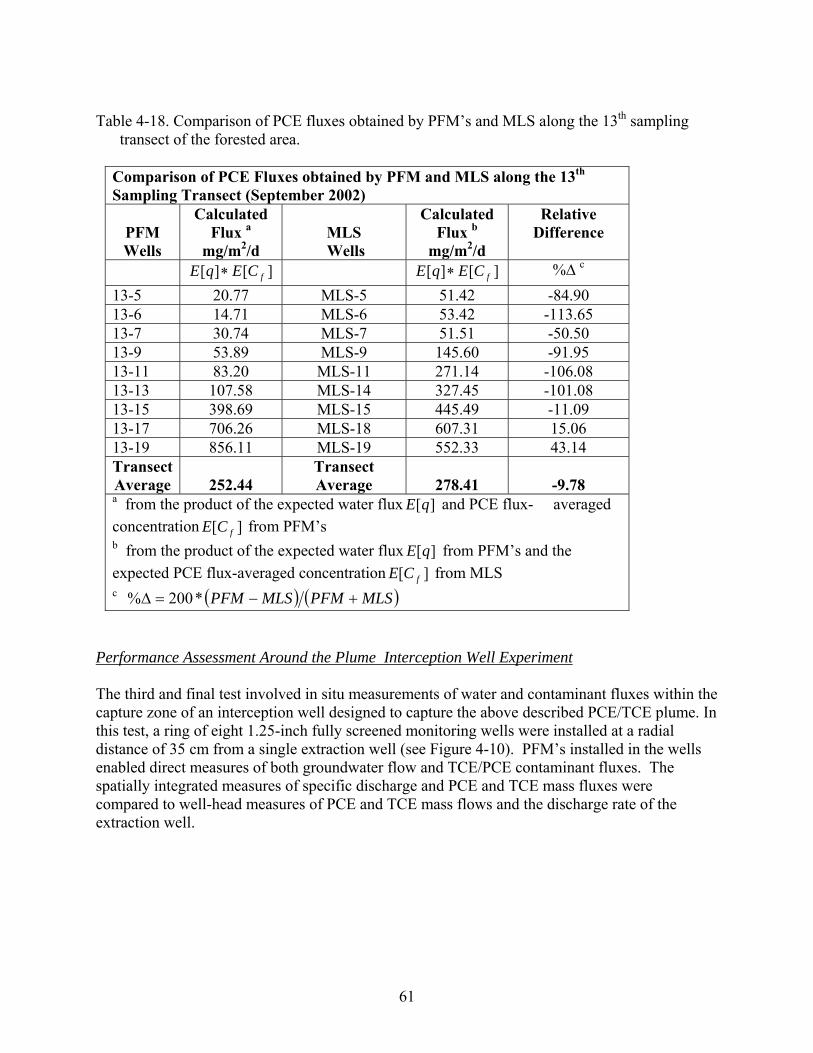
Table 4-18. Comparison of PCE fluxes obtained by PFM’s and MLS along the 13th sampling transect of the forested area.

Comparison of PCE Fluxes obtained by PFM and MLS along the 13th Sampling Transect (September 2002)

PFM Wells

Calculated Flux a

mg/m2/d

MLS Wells

Calculated Flux b

mg/m2/d

Relative Difference

][][ fCEqE ∗ ][][ fCEqE ∗ %∆ c

13-5 20.77 MLS-5 51.42 -84.90 13-6 14.71 MLS-6 53.42 -113.65 13-7 30.74 MLS-7 51.51 -50.50 13-9 53.89 MLS-9 145.60 -91.95 13-11 83.20 MLS-11 271.14 -106.08 13-13 107.58 MLS-14 327.45 -101.08 13-15 398.69 MLS-15 445.49 -11.09 13-17 706.26 MLS-18 607.31 15.06 13-19 856.11 MLS-19 552.33 43.14 Transect Average 252.44

Transect Average 278.41 -9.78

a from the product of the expected water flux and PCE flux- averaged concentration from PFM’s

][qE

)

][ fCEb from the product of the expected water flux from PFM’s and the expected PCE flux-averaged concentration from MLS

][qE][ fCE

c ( ) ( MLSPFMMLSPFM +−=∆ *200% Performance Assessment Around the Plume Interception Well Experiment The third and final test involved in situ measurements of water and contaminant fluxes within the capture zone of an interception well designed to capture the above described PCE/TCE plume. In this test, a ring of eight 1.25-inch fully screened monitoring wells were installed at a radial distance of 35 cm from a single extraction well (see Figure 4-10). PFM’s installed in the wells enabled direct measures of both groundwater flow and TCE/PCE contaminant fluxes. The spatially integrated measures of specific discharge and PCE and TCE mass fluxes were compared to well-head measures of PCE and TCE mass flows and the discharge rate of the extraction well.

61

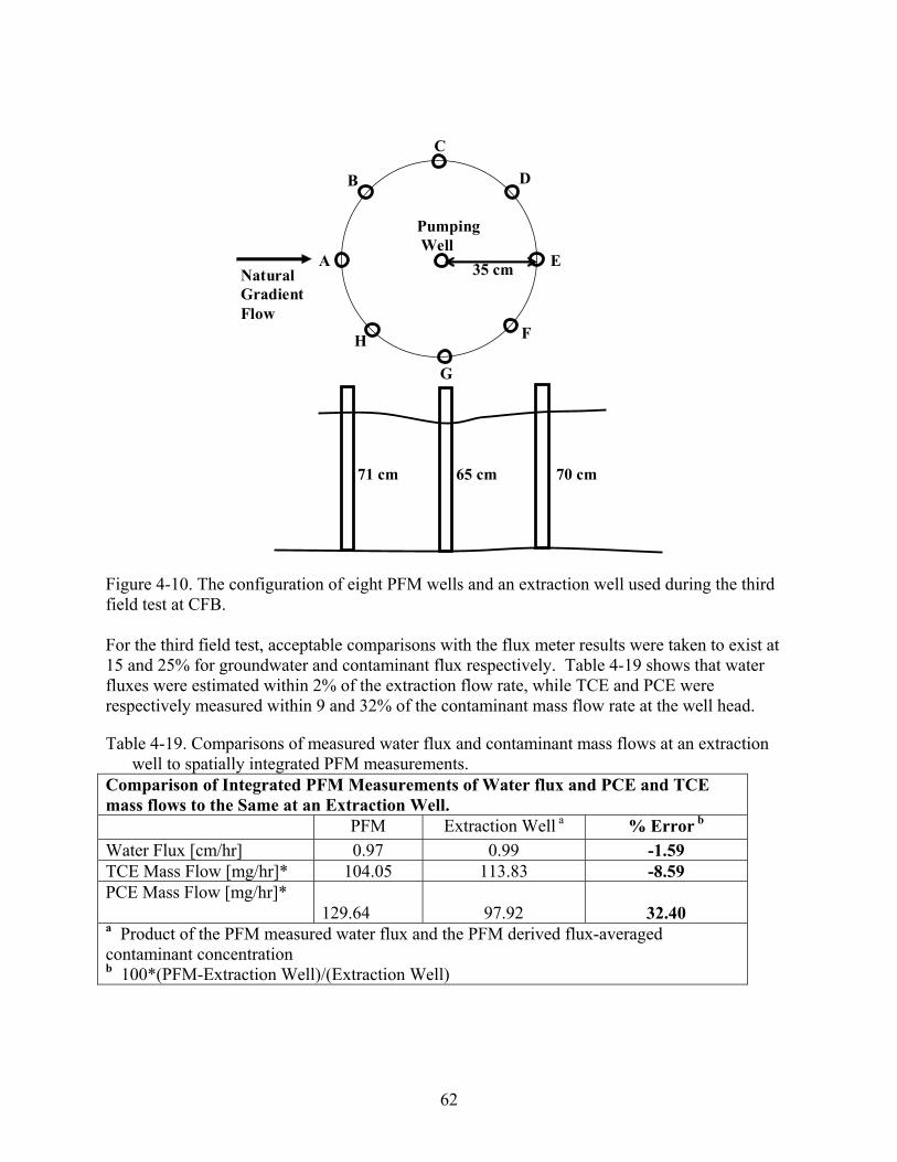
A

B D

C

H

G

F

E

Pumping Well

Natural Gradient Flow

35 cm

71 cm 70 cm65 cm

Figure 4-10. The configuration of eight PFM wells and an extraction well used during the third field test at CFB. For the third field test, acceptable comparisons with the flux meter results were taken to exist at 15 and 25% for groundwater and contaminant flux respectively. Table 4-19 shows that water fluxes were estimated within 2% of the extraction flow rate, while TCE and PCE were respectively measured within 9 and 32% of the contaminant mass flow rate at the well head.

Table 4-19. Comparisons of measured water flux and contaminant mass flows at an extraction well to spatially integrated PFM measurements.

Comparison of Integrated PFM Measurements of Water flux and PCE and TCE mass flows to the Same at an Extraction Well. PFM Extraction Well a % Error b

Water Flux [cm/hr] 0.97 0.99 -1.59 TCE Mass Flow [mg/hr]* 104.05 113.83 -8.59 PCE Mass Flow [mg/hr]*

129.64 97.92 32.40 a Product of the PFM measured water flux and the PFM derived flux-averaged contaminant concentration b 100*(PFM-Extraction Well)/(Extraction Well)

62

5.0. Cost Assessment 5.1 Cost Reporting

The passive flux meter is the only technology that provides simultaneous measurements of both water and contaminant fluxes. The most prominent alternative technology is to measure groundwater contaminant concentrations through multilevel samplers (MLS) and then calculate contaminant fluxes using groundwater fluxes estimated from borehole dilution (BHD) tests. This combined BHD/MLS method is the only alternative that provides depth varying estimates water and contaminant fluxes that can be compared to direct measurements provided by PFMs.

To evaluate costs of using PFMs and BHD/MLS method for site characterization, we follow the guidelines of the EPA document “Innovation in Site Characterization: Interim Guide to Preparing Case Studies” (EPA-542-B-98-009). We report costs associated with the passive flux meter and the alternative BHD/MLS method. Reported fixed costs include general categories of capital costs needed for PFM deployment in regards to planning and preparation. In addition, we report operational and variable costs including costs associated with per diem, labor, consumables, training,mobilization/demobilization, residual waste handling, sampling, and analysis. Finally, costs are expressed in totals, per linear foot, and where appropriate per sample. Many of the costs associated with the alternative technology are the same as those identified for the passive flux meter and are included in cost comparisons. The BHD/MLS method has some capital and training expenses associated with purchasing and using equipment to perform borehole dilution tests and with acquiring equipment to collect multilevel samples. Both PFMs and the BHD/MLS method require fully screened wells, and therefore the cost of installation for these is the same and not considered in this analysis. Also, the additional cost of installing multilevel samplers is not considered. 5.2. Cost Analysis

The major categories of costs that have been tracked are provided in Tables 5-1 and 5-2 for the two technologies of characterizing subsurface water and contaminant fluxes. To create these tables, we assume PFMs are deployed in 10 wells each having a screen interval of 10 feet. This represents 100 linear feet of well screen. PFMs are constructed in five-foot long units; therefore, 20 PFMs are deployed. The vertical sampling interval for the PFMs is assumed to be one foot; thus, a total of 100 data points of both Darcy and contaminant flux results are generated. Table 5-2 provides cost estimates for the alternative technology, BHD/MLS. Here again we assume a network of 10 wells in which multiple BHD tests are performed to measure Darcy fluxes at 10 depths over each well screen. In addition, at each well location MLSs are used to gather groundwater water samples at the same 10 depths for subsequent water quality analyses. Thus, from 10 wells the BHD/MLS method produces a total of 100 flux measurements by BHD and 100 aqueous contaminant concentrations from MLSs.

63

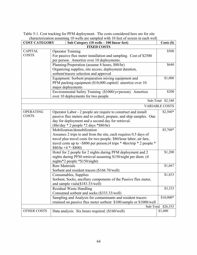
Table 5-1. Cost tracking for PFM deployment. The costs considered here are for site characterization assuming 10 wells are sampled with 10 feet of screen in each well.

COST CATEGORY Sub Category (10 wells – 100 linear feet) Costs ($) FIXED COSTS

Operator Training For passive flux meter installation and sampling. Cost of $2500 per person. Amortize over 10 deployments.

$500

Planning/Preperation (assume 8 hours, $80/hr) Organizing supplies, site access, deployment duration, sorbent/tracers selection and approval

$640

Equipment: Sorbent preparation mixing equipment and PFM packing equipment ($10,000 capitol) amortize over 10 major deployments

$1,000

CAPITAL COSTS

Environmental Safety Training ($1000/yr/person). Amortize over 10 deployments for two people

$200

Sub-Total $2,340VARIABLE COSTS

Operator Labor - 2 people are require to construct and install passive flux meters and to collect, prepare, and ship samples. One day for deployment and a second day for retrieval. (8hr/day * 2 people *2 days *$80/hr)

$2,560*

Mobilization/demobilization Assumes 2 trips to and from the site, each requires 0.5 days of travel plus travel costs for two people. $80/hour labor, air fare, travel costs up to ~$800 per person.(4 trips * 4hrs/trip * 2 people * $80/hr +4 *~$800)

$5,760*

Hotel for 2 people for 2 nights during PFM deployment and 2 nights during PFM retrieval assuming $150/night per diem. (4 nights*2 people *$150/night)

$1,200

Raw Materials Sorbent and resident tracers ($166.70/well)

$1,667

Consumables, Supplies Sorbent, Socks, ancillary components of the Passive flux meter, and sample vials($183.33/well)

$1,833

Residual Waste Handling Consumed sorbent and socks ($333.33/well)

$3,333

OPERATING COSTS

Sampling and Analysis for contaminants and resident tracers retained on passive flux meter sorbent $100/sample or $1000/well

$10,000*

Sub-Total $26,353OTHER COSTS Data analysis. Six hours required. ($160/well) $1,600

64

Sub-Total $30,293TOTAL TECHNOLOGY COST $30,293 Unit Cost per linear foot (ft) $303/ft * Mobilization/demobilization, labor and analytical costs can vary up to 50% as principal cost drivers

65

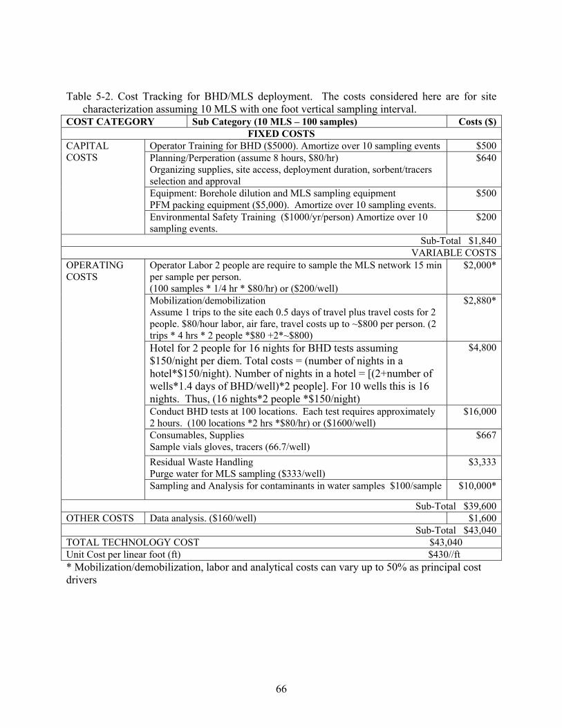
Table 5-2. Cost Tracking for BHD/MLS deployment. The costs considered here are for site characterization assuming 10 MLS with one foot vertical sampling interval.

COST CATEGORY Sub Category (10 MLS – 100 samples) Costs ($) FIXED COSTS

Operator Training for BHD ($5000). Amortize over 10 sampling events $500Planning/Perperation (assume 8 hours, $80/hr) Organizing supplies, site access, deployment duration, sorbent/tracers selection and approval

$640

Equipment: Borehole dilution and MLS sampling equipment PFM packing equipment ($5,000). Amortize over 10 sampling events.

$500

CAPITAL COSTS

Environmental Safety Training ($1000/yr/person) Amortize over 10 sampling events.

$200

Sub-Total $1,840VARIABLE COSTS

Operator Labor 2 people are require to sample the MLS network 15 min per sample per person. (100 samples * 1/4 hr * $80/hr) or ($200/well)

$2,000*

Mobilization/demobilization Assume 1 trips to the site each 0.5 days of travel plus travel costs for 2 people. $80/hour labor, air fare, travel costs up to ~$800 per person. (2 trips * 4 hrs * 2 people *$80 +2*~$800)

$2,880*

Hotel for 2 people for 16 nights for BHD tests assuming $150/night per diem. Total costs = (number of nights in a hotel*$150/night). Number of nights in a hotel = [(2+number of wells*1.4 days of BHD/well)*2 people]. For 10 wells this is 16 nights. Thus, (16 nights*2 people *$150/night)

$4,800

Conduct BHD tests at 100 locations. Each test requires approximately 2 hours. (100 locations *2 hrs *$80/hr) or ($1600/well)

$16,000

Consumables, Supplies Sample vials gloves, tracers (66.7/well)

$667

Residual Waste Handling Purge water for MLS sampling ($333/well)

$3,333

OPERATING COSTS

Sampling and Analysis for contaminants in water samples $100/sample $10,000*

Sub-Total $39,600OTHER COSTS Data analysis. ($160/well) $1,600

Sub-Total $43,040TOTAL TECHNOLOGY COST $43,040 Unit Cost per linear foot (ft) $430//ft * Mobilization/demobilization, labor and analytical costs can vary up to 50% as principal cost drivers

66

By varying the principal cost drivers of tables 5.1 and 5.2 which include mobilization - demobilization, labor, and analytical costs, the cost impacts can be determined. A 50% percent increase or decrease in each of these estimated drivers would alter the PFM total costs by ~33%. Similarly, a 50% increase or decrease in each of these estimated drivers for the MLS/BDH costs would alter the total cost by ~20%. Therefore, the unit cost per linear foot for the PFM method could range from $202 to $404; the unit cost per linear foot for the MLS/BDH method could range from $344 to $516. Because both PFMs and the BHD/MLS method involve short-term (less than 1 year) field operations, costs have not been discounted. 5.3 Cost Comparison Cost estimates per linear foot for PFM deployments and BHD/MLS measurements indicate that the PFM method results in lower unit costs depending on cost variability and the number of wells monitored. Both approaches exhibit similar costs in terms of materials and analytical costs and these costs are scalable to larger and smaller deployments. Figure 5.1 shows costs per linear foot for PFMs and the BHD/MLS method as a function of number of wells monitored. For sites involving 5 or more wells, PFMs are less expensive. When monitoring involves as few as 3 to 4 wells, costs are comparable; however, contaminant flux values derived from the BHD/MLS method represent short-term evaluations that reflect current conditions and not long-term trends. Therefore, in the absence of continuous monitoring, it may be more cost effective and in the best interests of stakeholders to deploy systems designed to gather cumulative measures of water flow and contaminant mass flow. Cumulative monitoring devices generate the same information derived from integrating continuous data. These systems should produce robust flux estimates that reflect long-term transport conditions and are less sensitive to day-to-day fluctuation in flow and contaminant concentration. Another major advantage over the BHD/MLS method results from the lengthy time required to collect samples from MLS and to conduct borehole dilutions on site. Some cost savings may be realized by automating the borehole dilution method such that one operator can conduct multiple tests simultaneously. Also, the estimation of 2 hours per BHD test may be appropriate for sites with average or high groundwater velocities, but may be too small for lower velocity sites. Obviously, site specific conditions can lead to changes in the cost estimates. In general, conducting BHD tests demands considerably more time on-site than PFMs, and they may be impractical to conduct when more than 7-10 wells are involved.

67

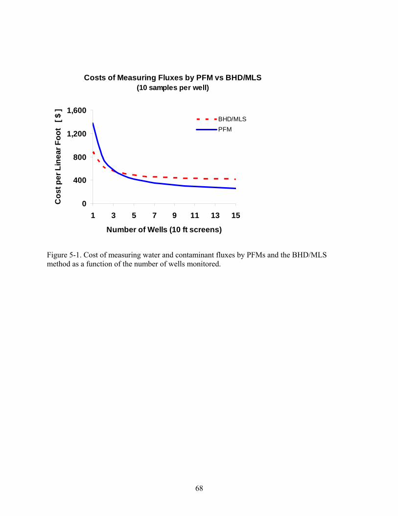
Costs of Measuring Fluxes by PFM vs BHD/MLS(10 samples per well)

0

400

800

1,200

1,600

1 3 5 7 9 11 13 15

Number of Wells (10 ft screens)

Cos

t per

Lin

ear F

oot

[ $

]

BHD/MLSPFM

Figure 5-1. Cost of measuring water and contaminant fluxes by PFMs and the BHD/MLS method as a function of the number of wells monitored.

68

6.0. Implementation Issues 6.1. Environmental Checklist Permission to introduce small quantities of tracers was obtained through the University of Waterloo, from on-Base managers of the research site. The University of Florida is currently working on the development of a flux meter with a sorbent annulus to retain all tracer mass within meter. Furthermore, Campbell et al. (2006) and Klammler et al. (2006b) present new flux meter designs that retain resident tracers. 6.2. Other Regulatory Issues Contact with appropriate on-Base managers was initiated by University of Waterloo. Contact with Base personnel and users of the technology continued throughout the project in order to avoid any problems in regulation.. 6.3. End-User Issues The technology was very simple to construct and implement. We have experienced only minimal issues for transfer to end-users. Installations used in the demonstration were similar to the anticipated final product. As we continue technology deployments, refinements will be made and applied to future installations of the flux meter. These refinements may be site specific.

69

7.0. References

Annable, M.D., Hatfield, K., Cho, J., Klammler, H., Parker, B., Cherry, J., and. Rao. P.S.C., 2005. “Field-scale evaluation of the passive flux meter for simultaneous measurment of groundwater and contaminant fluxes.” Environ. Sci. and Technol. Environ. Sci. Technol., 39 (18), 7194 -7201. Bahr, J.M., and Rubin, J., 1987. Direct comparison of kinetic and local equilibrium formulation for solute transport affected by surface reactions, Water Resour. Res., 23(3), 438-452. Basu, N., P.S.C. Rao, I.C. Poyer, M.D. Annable, and K. Hatfield. 2006. Flux based assessment at a site contaminated with trichloroethylene, Journ. Contam. Hydrol., 86 (1-2), 105-12. Bockelmann, A., Ptak, T., Teutsch, G., 2001. An analytical quantification of mass fluxes and natural attenuation rate constants at a former gasworks site. J. Contam. Hydrol., 53, 429-453. Broholm, K., Feenstra, S., and Cherry, J.A. (1999). Solvent release into a sandy aquifer. 1. Overview of source distribution and dissolution behaviour. Environmental Science & Technology, 33:5 pp. 681-690. Brusseau, M.L., and Rao, P.S.C., 1989. The influence of sorbate-organic matter interactions on sorption nonequilibrium. Chemosphere, 18(9/10):1691-1706. Campbell, T. J., K. Hatfield, H. Klammler, M. D. Annable, and P.S.C. Rao. 2006. Magnitude and directional measures of water and Cr(VI) fluxes by passive flux meter. Environmental Science and Technology, 40, 6392-6397. Cherry, J.A., Barker, J.F., Feenstra, S., Gillham, R.W., Mackay, D.M., Smyth, D.J.A. (1996). Borden site for groundwater contamination experiments: 1978-1995. In: Kobus, H., Barczewsdi, D., Koschitzky, H.-P. (eds) Groundwater and Subsurface Remediation- Research Strategies for In-Situ Remediation, Springer-Verlos, Berlin, pp 101-127. Drost, W., Klotz, D., Koch, A., Moser, H., Neumaier, F., and Rauert, W., 1968. Point dilution methods of investigating ground water flow by means of radioisotopes. Water Resour. Res. 4 (1), 125-146. Feenstra, S., Cherry, J.A., and Parker, B.L., 1996. Conceptual models for the behavior of nonaqueous phase liquids (DNAPLs) in the subsurface. In: J.F. Pankow and J.A. Cherry (Eds.), Dense Chlorinated Solvents and Other DNAPLs in Groundwater. Waterloo Press, Portland OR, pp. 53-88. Fetter, C.W., 1999. Contaminant Hydrology, Second Edition, Prentice Hall, Upper Saddle River, NJ, pp.125-127.

70

Hatfield, K., Annable, M., Cho, J., Rao, P.S.C., and Klammler. H. 2004. “A direct passive method for measuring water and contaminant fluxes in porous media,” Journal of Contaminant Hydrology, Vol 75 (3-4), 2004, 155-181. Hatfield, K., Rao, P.S.C., Annable M.D., and Campbell T., 2002a. Device and method for measuring fluid and solute fluxes in flow systems, Patent US 6,402,547 B1. Hatfield , K., Annable, M.D., Kuhn, S., Rao, P.S.C, and Campbell, T.J. 2002b. A new method for quantifying contaminant flux at hazardous waste sites, In: Thorton, S. and Oswald S. (eds) Groundwater Quality 2001, Third International Conference on Groundwater Quality, University of Sheffield, United Kingdom. Heyse, E., Augustijn, D., Rao, P.S.C., and Delfino, J.J., 2002. Nonaqueous phase liquid dissolution and soil organic matter sorption in porous media: Review of system simlarities. Critical Reviews in Environmental Science and Technology, 32(4), 337-397. Klammler, H K. Hatfield, M. Annable, E. Agyei, B. Parker, J. Cherry, and P.S.C. Rao. 2006a. General analytical treatment of the flow field relevant for passive fluxmeter interpretation. Water Resour. Res. (In Press). Klammler, H., K. Hatfield, and M. Annable. 2006b. Concepts for measuring horizontal groundwater flow directions using the passive flux meters. Advances in Water Resources (In Press). Labaky, W. 2004. Theory and testing of a device for measuring point-scale groundwater velocities. Ph.D. Thesis, Department of Earth Sciences, University of Waterloo, Waterloo, Ontario, Canada. Laukonen, K.A., Parker, B.L., Cherry, J.A. 2000. Internal characteristics of a bromide tracer zone during natural flow in the Borden aquifer, Ontario, Canada. Tracers and Modeling in Hydrogeology, Proceedings of the TraM'2000 Conference, Liege, Belgium, May 2000, IAHS Publ. No. 262, pp 227-233. Newman, M., K. Hatfield, J. Hayworth, P.S.C. Rao, and T. Stauffer. 2005. A hybrid method for inverse characterization of subsurface contaminant flux. Journal of Contaminant Hydrology, 81(1-4), 34-62. Newman, M., K. Hatfield, J. Hayworth, P.S.C. Rao, and T. Stauffer. 2006. Inverse characterization of NAPL source zones. Environmental Science and Technology, 40(19), 6044-6050. Ogilvi, N.A., 1958. An electrolytical method for determining the filtration velocity of underground waters. Bull. Sci.-Tech. Inf., 4 (16), Gosgeoltekhizdat, Moscow.

71

Strack, O.D.L. and Haitjema, H.M., 1981. Modeling double aquifer flow using a comprehensive potential and distribution singularities: 2. Solution for inhomogeneous permeabilities. Water Resour. Res. 17(5), 1551-1560. Thibodeaux, L.J., 1996. Environmental Chemodyanmics; Movement of Chemicals in Air, Water, and Soil. 2nd Edition, John Wiley & Sons, Inc. New York, pp 278. USEPA, 1998. Technical Protocol for Evaluating Natural Attenuation of Chlorinated Solvents in Ground Water, EPA/600/R-98/128, September. Yaron, B., 1978. Some aspects of surface interactions of clays with organophosphorous pesticides. Soil Science. 125, 210-16.

72

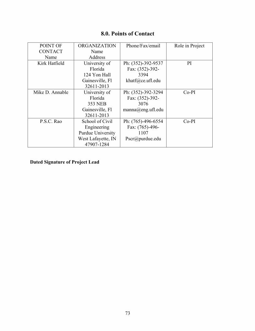
8.0. Points of Contact

POINT OF CONTACT

Name

ORGANIZATION Name

Address

Phone/Fax/email Role in Project

Kirk Hatfield University of Florida

124 Yon Hall Gainesville, Fl

32611-2013

Ph: (352)-392-9537 Fax: (352)-392-

3394 [email protected]

PI

Mike D. Annable University of Florida

353 NEB Gainesville, Fl

32611-2013

Ph: (352)-392-3294 Fax: (352)-392-


Co-PI

P.S.C. Rao School of Civil Engineering

Purdue University West Lafayette, IN

47907-1284

Ph: (765)-496-6554 Fax: (765)-496-


Co-PI

Dated Signature of Project Lead

73

Appendix A: Analytical Methods Supporting the Experimental Design STANDARD OPERATING PROCEDURE FOR ANALYSIS OF ALCOHOL TRACERS (November 15, 1995) SCOPE AND APPLICATION 1. This SOP describes the analytical procedures utilized by the Soil and Water Science Department, University of Florida, IFAS, for analysis of alcohols used as partitioning tracers in both lab and field studies in order to quantify the amount and distribution of residual non-aqueous phase liquids (NAPLs) present in the saturated zone. 2. This SOP was written by R.D. Rhue, Soil and Water Science Department, University of Florida, Gainesville, Fl. It is a modification of SOP-UF-Hill-95-07-0010-v.2, prepared by D.P. Dai, H.K. Kim, and P.S.C. Rao, Soil and Water Science Department, University of Florida. The SOP of Dai, Kim, and Rao was modified from a protocol provided to them by Professor Gary Pope at the University of Texas-Austin. 3. The alcohol tracers used in the UF lab and field studies are ethanol, n-butanol, n-pentanol, n-hexanol, n-heptanol, 2,2-dimethyl-3-pentanol, and 6-methyl-2-heptanol. 4. The method involves gas chromatography (GC) analysis for alcohol concentrations in aqueous samples. A flame-ionization detector (FID) is used to quantify the analyte concentrations in the sample. The method has been found to provide reliable and reproducible quantitation of alcohols for concentrations > 1 ug/mL. This value may be considered the minimum detection level (MDL). The standard calibration curve for FID response has been found to be linear up to 3,000 ug/mL for ethanol. 5. Samples selected for GC-FID analysis may be chosen on the basis of preliminary screening which will provide approximate concentration ranges and appropriate sample injection volumes, standard concentrations, etc. PURPOSE The purpose of this SOP is to insure reliable and reproducible analytical results for alcohols in aqueous samples for laboratory-based or on-site (field-based) GC-FID analyses, and to permit tracing sources of error in analytical results. PROCEDURES 1. Sample Containers, Collection, Transportation and Storage

74

Sample Containers: Field samples will be collected in 5-mL glass sample vials (Fisher Catalog # 06-406-19F) with teflon-faced septa caps. Glass vials and caps are not reused. Sample Collection: Each field sample vial will be completely filled with liquid, such that no gas headspace exists, and capped. The vials will not be opened until the time for analysis. Transportation and Storage: Field samples will be stored in coolers containing "blue ice", and later stored in refrigerators in a trailer located on the site. Samples may be subjected to on-site GC analysis, and/or shipped back to UF labs; samples will be packed in coolers and shipped via overnight air express (e.g., FedEx). The samples will be stored in the cold storage room or refrigerator at 4C, until GC analysis. After sub-sampling, the samples are returned to cold storage. For lab studies, samples will be collected directly in 2 mL GC vials whenever possible and stored in a refrigerator if analysis is expected to take more than a day. 2. Sub-sampling and Dilution Field samples will be sub-sampled into 2-ml vials for automated GC analysis. Disposable, Pasture glass pipets (Fisher Catalog # 13-678-20B) will be used to transfer samples from 5-mL sample vials to the 2-mL GC vials. For samples needing dilution prior to GC analysis, a dilution of 1:10 should be sufficient. Dilutions will be made using double-distilled, deionized water. 3. Apparatus and Materials Glassware: Disposable micro-pipets (100 uL; Fisher Catalog # 21-175B; 21-175F) and Class A volumetric pipets (1 or 2 mL) are required for sample dilution. Disposable Pasteur glass pipets (Fisher Catalog # 13-678-20B) are required for sub-sampling. GC vials (2-mL) with Teflon-faced caps (Fisher Catalog # 03-375-16A) are required for GC analysis. Volumetric class A pipets and volumetric class A flasks are required for preparations of the calibration standards. Gas Chromatograph System: An analytical GC system with a temperature-programmable oven, auto-injector capable of on-column injection, and either an integrator or a PC-based data acquisition/analysis software system are required. Also required are other accessories, including analytical columns and the gases required for GC-FID operation.

75

A Perkin Elmer Autosystem with an FID and an integrated autosampler will be used for analysis of field and laboratory samples. The Perkin Elmer system will be linked to an IBM-compatible PC loaded with Turbochrom (version 4.01) software. A J&W Scientific DB-624 capillary column (30m X 0.53mm, 3m film thickness) will be used. Zero-grade air and ultra-high purity hydrogen will be used for the FID. Ultra-high purity nitrogen or helium will be used for carrier gas. 4. Reagents Deionized, Double-Distilled Water: Deionized, double distilled water is prepared by double distillation of deionized water in a quartz still. This water will be referred to as reagent water. Alcohols: Certified ACS grade alcohols will be purchased from Fisher Scientific and used as received. 5. Standard Solutions Stock Standard Solution: Analytical standards will be prepared from reagent chemicals by the laboratory. Stock standards each contain a single alcohol dissolved in reagent water and stored in 20 mL glass vials (Fisher Catalog # 03-393-D) with teflon-lined caps. These stock solutions will be kept in a refrigerator at 4 C. Fresh stock standards will be prepared every six months. The procedure for making stock standard solutions is essentially that given in the Federal Register, Rules and Regulations, Thursday, November 29, 1979, Part III, Appendix C, Section 5.10, "Standard Stock Solutions". The only modification of the procedure for the current study is that reagent water is used as the solvent in place of methanol. Calibration Standards: Calibration standards will be prepared by diluting the stock standards in reagent water. Each calibration standard will contain each of the alcohols listed above. Five concentrations will be prepared that cover the approximate concentration range utilized in the partitioning tracer experiments. 6. QC blank Spike/Matrix Spike

76

Two 1 mL aliquots of the sample to be spiked will be transferred to clean vials. To one vial, 1 mL of reagent water will be added. To the second vial, 1 mL of a calibration standard will be added. The spike recovery will be calculated using the difference between the two measured concentrations and the known spike concentration. 7. Quality Control GC injector septa will be changed every 80 to 100 injections, or sooner if any related problems occur. Injector liner will be cleaned or changed every 80 to 100 injections or sooner if any related problems occur. A method blank will be included in every 50 samples A complete set of calibration standards (5) will be run at the beginning of each day and after every fiftieth sample. One standard and a blank will be included in every 25 samples. A sample spike and a blank spike will be included in every 50 samples. 8. Instrumental Procedures Gas Chromatography: For J&W DB-624 Column: Injection port temperature 200C FID detector temperature 225C Temp Program: Isothermal at 60C for 0 min; Ramp to 120C at 5 C/min. 9. Sample Preparation Sub-sampling: Field samples will be transferred from the 5 mL sample vials to the 2 mL GC vials and capped with open-top, teflon-lined septa caps. Dilution: Samples will be diluted if chromatographic peak areas for any of the alcohols exceed those of the highest calibration standard. One mL of sample will be added to an appropriate amount of reagent water to make the dilution. 10. Sample Analysis Analysis: The samples will be allowed to reach ambient temperature prior to GC analysis.

77

Sample vials (2 mL) will be loaded onto the Perking Elmer GC auto-injector. A one uL injection volume will be used for both samples and standards. Analyte Identification: Analyte identification will be based on absolute retention times. The analytes of interest should elute at their characteristic retention times within 0.1 minute for the automated GC system. Analyte Quantitation: When an analyte has been identified, the concentration will be based on the peak area, which is converted to concentration using a standard calibration curve. 11. Interferences Contamination by carry-over can occur whenever high-level and low-level samples are sequentially analyzed. To reduce carry over, the injector syringe should rinsed with reagent water between samples. Potential carry-over will be checked by running a highly concentrated sample, but one still within the standard concentration range, followed by a blank. A negligible reading for the blank will insure that carry-over has been minimized. 12. Safety The main safety issue concerning the use of the GC at a field site relates to the compressed gases. The FID gases (hydrogen and air) form explosive mixtures. It is important to keep this in mind at all times, and be aware of the hazard potential in the event of an undetected hydrogen leak. All gas connections will be properly leak tested at installation. High-pressure compressed-gas cylinders will be secured to a firm mounting point, whether they are located internally or externally. Gas cylinders should preferably be located outside the trailer on a flat, level base, and the gas lines run inside through a duct or window opening. If the gases are located outside, then some form of weatherproofing for the gauges will be necessary. As a temporary measure, heavy-duty polyethylene bags, secured with tie-wraps, have been used successfully; this may not be very elegant but it is very effective for short-term use of the GC. A more permanent protective housing must be built if the GC is located at the trailer for an extended time period. The main operating drawback to locating the gas cylinders externally is that it is not easy to monitor the cylinder contents from inside. The gas which could be used up most quickly is air for the FID, particularly if two instruments are hooked up to the same supply and they are running continuously. A reserve cylinder of air should be available at all times to prevent down time. If it is not possible to arrange external citing easily, the gas cylinders should be secured to a wall inside the trailer.

78

It is a good laboratory operating practice to make sure the flame is attended at all times. When it is necessary to change the injection liner on the GC, the detector gases should be shut off. The column must be connected to the detector before igniting the flame. The trailer should be kept well ventilated when using the GC. Reference to the Materials Safety Data Sheets (MSDS) will be made for information on toxicity, flammability, and other hazard data.

79

STANDARD OPERATING PROCEDURE FOR ANALYSIS OF TARGET ANALYTES IN GROUNDWATER SAMPLES (February 20, 1996) SCOPE AND APPLICATION 1. This SOP describes the analytical procedures utilized by the Department of Environmental Engineering Sciences, University of Florida, for analysis of target analytes in groundwater samples from both lab and field studies. This analysis provides characterization of existing site and lab column aqueous contamination both before and following flushing technology applications. 2. This SOP was written by M.D. Annable, Department of Environmental Engineering Sciences, University of Florida, Gainesville, FL. It is a modification of SOP-UF-Hill-95-07-0012-v.2, prepared by D.P. Dai and P.S.C. Rao, Soil and Water Science Department, University of Florida. 3. The selected constituents are benzene, toluene, o-xylene, 1,1,1-trichloroethane, 1,3,5,-trimethylbenzene, 1,2-dichlorobenzene, decane, and naphthalene. 4. The method involves gas chromatography (GC) analysis for target analyte concentrations in aqueous samples. Headspace analysis with a flame-ionization detector (FID) is used to quantify the analyte concentrations in the sample. The method has been found to provide reliable and reproducible quantitation of the above constituents for concentrations > 5 ug/L. This value may be considered the method detection level (MDL). 5. Samples selected for GC-FID analysis may be chosen on the basis of preliminary screening which will provide approximate concentration ranges and appropriate sample injection times, and standard concentrations, etc. PURPOSE The purpose of this SOP is to insure reliable and reproducible analytical results for soluble NAPL constituents in aqueous samples for laboratory-based GC-FID analyses, and to permit tracing sources of error in analytical results. PROCEDURES 1. Sample Containers, Collection, Transportation and Storage Sample Containers: Field samples will be collected in 20-mL glass sample vials (Fisher Catalog # 03-340-121) with teflon-faced rubber backed caps. Glass vials and caps are not reused. Sample Collection: Each field sample vial will be completely filled with liquid, such that no gas headspace exists, and capped. The vials will not be opened until the time for analysis.

80

Transportation and Storage: Field samples will be stored in coolers containing "blue ice", and later stored in refrigerators in a trailer located on the site. Samples will be sent to UF labs packed in coolers and shipped via overnight air express (e.g., FedEx). The samples will be stored in the cold storage room or refrigerator at 4C, until GC analysis. After sub-sampling, the samples are returned to cold storage. For lab studies, samples will be collected directly in 20 mL Headspace vials whenever possible and stored in a refrigerator if analysis is expected to take more than a day. 2. Sub-sampling and Dilution Field samples will be sub-sampled placing 10-ml into 20-ml headspace vials containing 2 g of sodium chloride for automated GC analysis. Pipets will be used to transfer samples from 20-mL sample vials to the 20-mL GC headspace vials. 3. Apparatus and Materials Glassware: Glass pipets are required for sub-sampling. GC headspace vials (20-mL) with Teflon-faced caps are required for GC analysis. Volumetric class A pipets and volumetric class A flasks are required for preparations of the calibration standards. Gas Chromatograph System: An analytical GC system with a temperature-programmable oven, headspace sample injection system, and either an integrator or a PC-based data acquisition/analysis software system are required. Also required are other accessories, including analytical columns and the gases required for GC-FID operation. A Perkin Elmer Autosystems with an HS40 Auto-headspace sampler and a FID will be used for analysis of field and laboratory samples. The Perkin Elmer system will be linked to an IBM-compatible PC loaded with Turbochrom (version 4.01) software. A J&W Scientific DB-624 capillary column (50m X 0.53mm, 3m film thickness) will be used. Zero-grade air and high purity hydrogen will be used for the FID. Ultra-high purity nitrogen or helium will be used for carrier gas. 4. Reagents Deionized, Double-Distilled Water: Deionized, double distilled water is prepared by double distillation of deionized water in a quartz still. This water will be referred to as reagent water.

81

5. Standard Solutions Stock Standard Solution: Analytical standards will be prepared from reagent chemicals by the laboratory. Stock standards will each contain a single analyte dissolved in methanol and stored in 20 mL glass vials (Fisher Catalog # 03-393-D) with teflon-lined caps. These stock solutions will be kept in a refrigerator at 4 C. Fresh stock standards will be prepared every six months. The procedure for making stock standard solutions is essentially that given in the Federal Register, Rules and Regulations, Thursday, November 29, 1979, Part III, Appendix C, Section 5.10, "Standard Stock Solutions". Calibration Standards: Calibration standards will be prepared by diluting the stock standards in water. Each calibration standard will contain each of the eight analytes listed above. Five concentrations will be prepared that cover the approximate concentration range from 0 to 20 mg/L. 6. QC blank Spike/Matrix Spike Two 1 mL aliquots of the sample to be spiked will be transferred to clean vials. To one vial, 1 mL of reagent water will be added. To the second vial, 1 mL of a calibration standard will be added. The spike recovery will be calculated using the difference between the two measured concentrations and the known spike concentration. 7. Quality Control A method blank will be included in every 50 samples A complete set of calibration standards (5) will be run at the beginning of each day and after every fiftieth sample. One standard and a blank will be included in every 25 samples. A sample spike and a blank spike will be included in every 50 samples. 8. Instrumental Procedures Gas Chromatography: For J&W DB-624 Column: Headspace sample temperature 90C Injection needle temperature 100C Transfer line Temperature 110C FID detector temperature 225C Carrier gas pressure 8psi Temp Program: Isothermal at 50C for 0 min; Ramp to 200C at 5 C/min; hold for 10 min.

82

9. Sample Preparation Sub-sampling: Field samples will be transferred from the 20 mL sample vials to the 20 mL GC headspace vials and capped with open-top, teflon-lined septa caps. Dilution: Samples will be diluted if chromatographic peak areas for any of the analytes exceed those of the highest calibration standard. One mL of sample will be added to an appropriate amount of reagent water to make the dilution. 10. Sample Analysis Analysis: Sample headspace vials (20 mL) will be loaded onto the Perking Elmer HS40 auto-sampler. Samples will be pressurized for 1 min followed by a 0.1 minute injection time and a withdrawal time of 0.5 minute. Analyte Identification: Analyte identification will be based on absolute retention times. The analytes of interest should elute at their characteristic retention times within ±0.1 minute for the automated GC system. Analyte Quantitation: When an analyte has been identified, the concentration will be based on the peak area, which is converted to concentration using a standard calibration curve. 11. Interferences Contamination by carry-over can occur whenever high-level and low-level samples are sequentially analyzed. To reduce carry over, the injector needle should purged with carrier gas between samples. Potential carry-over will be checked by running a highly concentrated sample, but one still within the standard concentration range, followed by a blank. A negligible reading for the blank will insure that carry-over has been minimized. 12. Safety The main safety issue concerning the use of the GC relates to the compressed gases. The FID gases (hydrogen and air) form explosive mixtures. It is important to keep this in mind at all times, and be aware of the hazard potential in the event of an undetected hydrogen leak. All gas connections will be properly leak tested at installation. High-pressure compressed-gas cylinders will be secured to a firm mounting point, whether they are located internally or externally.

83

When it is necessary to change the injection liner on the GC, the detector gases should be shut off. The column must be connected to the detector before igniting the flame. Reference to the Materials Safety Data Sheets (MSDS) will be made for information on toxicity, flammability, and other hazard data.

84

STANDARD OPERATING PROCEDURE FOR EXTRACTION OF ANALYTES FROM FLUX DEVICE SORBENTS (October 10, 2001) SCOPE AND APPLICATION 1. This SOP describes the procedures used by the Department of Environmental Engineering Sciences, University of Florida, for extraction of target analytes (including tracers) from sorbents used in flux devices inserted in monitoring wells. 2. This SOP was written by M.D. Annable, Department of Environmental Engineering Sciences, University of Florida, Gainesville, FL. 3. The selected constituents are TCE, PCE, and alcohol tracers: Methanol Ethanol 2-propanol (IPA) 2-methyl-1-propanol (IBA) 2-methyl-2-propanol (TBA) n-propanol n-butanol n-pentanol n-hexanol n-heptanol 3-heptanol n-octanol 2-octanol 2,4-dimethyl-3-pentanol 2-ethyl-1-hexanol 3,5,5-trimethyl-1-hexanol 6-methyl-2-heptanol 2,6-dimethyl-2-heptanol n-decane Potential Sorbents include: Liquid (mixed in a sand matrix at a pore volume saturation of 10%) Tetradecane Heptadecane Hexadecane Solid Activated Carbon

85

Surfactant modified zeolytes 4. The method involves liquid extraction in 20 or 40 ml VOA vials using organic solvents. PURPOSE The purpose of this SOP is to insure reliable and reproducible analytical results. Extracted constituents will be quantified suing analytical methods described in other SOPs. PROCEDURES 1. Sample Containers, Collection, Transportation and Storage Sample Containers: Field samples will be collected in 20-mL or 40-ml glass sample vials (Fisher Catalog # 03-340-121) with teflon-faced rubber backed caps. Sample Collection: Each field sample vial will be partially filled with the extraction solvent (alcohol IPA, IBA, etc. or Methylenechloride) using a pipet or repeating volume dispenser. Typically 10 or 20-ml of solvent will be used. Transportation and Storage: Field samples will be stored in coolers containing "blue ice", and later stored in refrigerators in a trailer located on the site. Samples will be sent to UF labs packed in coolers and shipped via overnight air express (e.g., FedEx). The samples will be stored in the cold storage room or refrigerator at 4C, until GC analysis. After sub-sampling, the samples are returned to cold storage. For lab studies, samples will be collected directly in 20 mL Headspace vials whenever possible and stored in a refrigerator if analysis is expected to take more than a day. 2. In the laboratory, samples will be rotated for a minimum of 8 hours on a rotator (Glas-Col model RD 4512). 3. Sub-sampling and Dilution Field samples will be sub-sampled into 2 ml GC vials. Pipets will be used to transfer samples from 20-mL sample vials to the 2-mL GC vials. 3. Apparatus and Materials Glassware: Glass pipets are required for sub-sampling. Safety

86

Gloves and eye protection will be worn during all extraction activities. Reference to the Materials Safety Data Sheets (MSDS) will be made for information on toxicity, flammability, and other hazard data.

87

Appendix E: Quality Assurance Project Plan (QAPP)

88

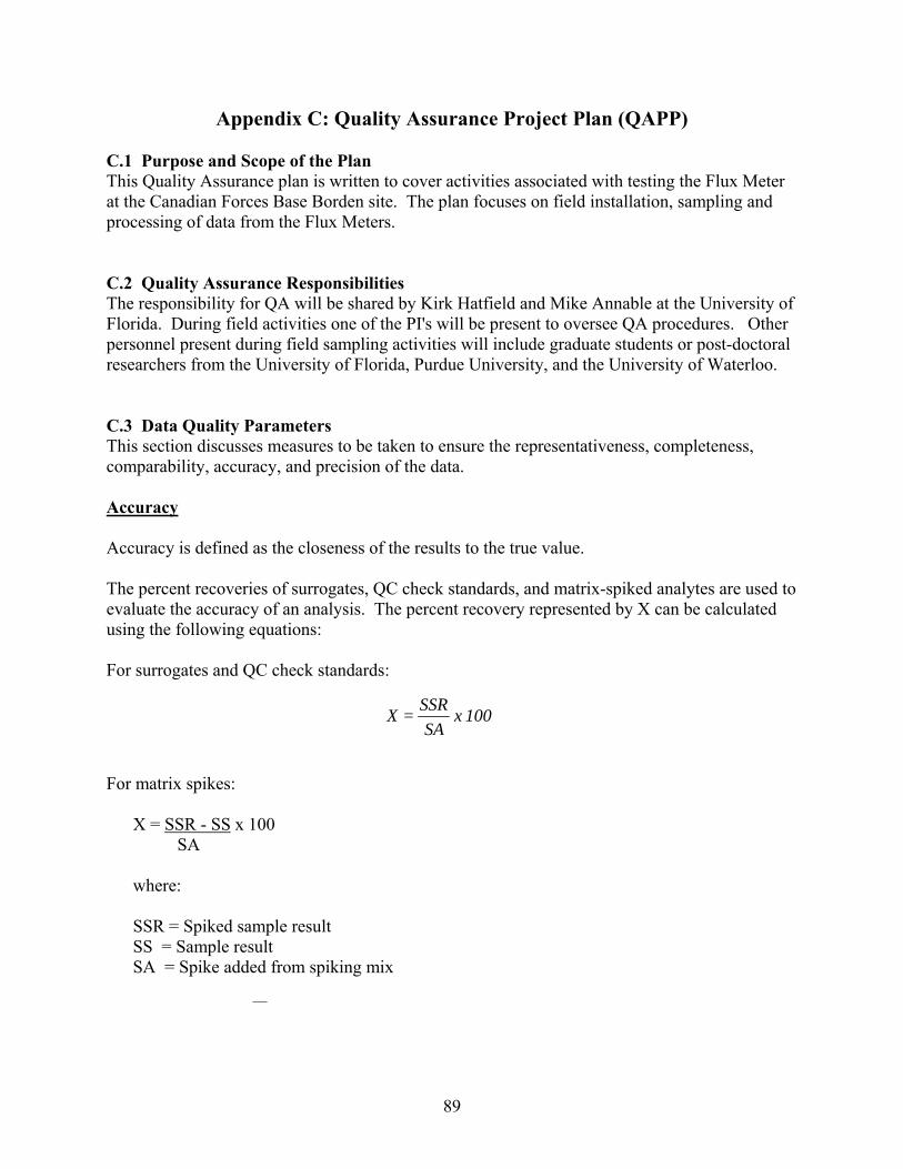
Appendix C: Quality Assurance Project Plan (QAPP) C.1 Purpose and Scope of the Plan This Quality Assurance plan is written to cover activities associated with testing the Flux Meter at the Canadian Forces Base Borden site. The plan focuses on field installation, sampling and processing of data from the Flux Meters. C.2 Quality Assurance Responsibilities The responsibility for QA will be shared by Kirk Hatfield and Mike Annable at the University of Florida. During field activities one of the PI's will be present to oversee QA procedures. Other personnel present during field sampling activities will include graduate students or post-doctoral researchers from the University of Florida, Purdue University, and the University of Waterloo. C.3 Data Quality Parameters This section discusses measures to be taken to ensure the representativeness, completeness, comparability, accuracy, and precision of the data. Accuracy Accuracy is defined as the closeness of the results to the true value. The percent recoveries of surrogates, QC check standards, and matrix-spiked analytes are used to evaluate the accuracy of an analysis. The percent recovery represented by X can be calculated using the following equations: For surrogates and QC check standards:

100 x SA

SSR = X

For matrix spikes: X = SSR - SS x 100 SA where: SSR = Spiked sample result SS = Sample result SA = Spike added from spiking mix

89

The mean percent recovery (X) is defined by:

N

X = X iN

1=i∑

where: Xi = The percent recovery value of a spike replicate N = Number of spikes Precision Precision is a measure of the mutual agreement among individual measurements of the same parameters under prescribed similar conditions. The analytical precision is determined using results from duplicate or replicate analyses of samples and from matrix spike results for a given matrix. The Relative Percent Difference (RPD) is used to evaluate the precision of duplicate analyses. Relative Percent Difference is defined in the following equation:

100 x x

X2) - 2(X1 = %RPD

X1 = First duplicate value X2 = Second duplicate value When replicate analyses are performed, precision is measured in terms of the Standard Deviation (SD) which is defined in the following equation:

⎥⎦

⎤⎢⎣

⎡∑

1-N)X - X( = S

2i

‰

N1=i

where: Xi = The recovery value of a spike replicate X = Arithmetic average of the replicate values N = Number of spikes

90

Completeness Completeness is defined as the percent of parameters falling within acceptance criteria and the results subsequently reported. A goal of 95 percent completeness has been set for all samples. The general requirement of this quality assurance program is to analyze a sufficient number of standards, replicates, blanks, and spike samples to evaluate results adequately against numerical QA objectives. C.4 Calibration Procedures, Quality Control Checks, and Corrective Action The focus of the following section is to describe initial and continuing calibration procedures for analytical instrumentation, duplicate and control testing and data reduction, validation, and reporting. Supplies and Quality Control Materials All supplies (i.e., glassware, chemicals, reagents) used will be of the best possible quality to ensure proper instrument calibration and avoid contamination. All reagents used are prepared from Analytical Reagent Grade (AR) chemicals or higher purity grades, unless such purity is not available. The preparation of all reagents will be documented, including source, mass, and dilutions. Each reagent will be clearly labeled with the composition, concentration, date prepared, initials of preparer, expiration date, and special storage requirements, if any. Reagents Reagent solutions are stored in appropriate glass, plastic, or metal containers. Reagents are stored under conditions designed to maintain their integrity (refrigerated, dark, etc.). Shelf life is listed on the label and the reagent is discarded after it has expired. Dry reagents such as sodium sulfate, silica gel, alumina, and glass wool are either muffled at 400°C or extracted with solvent before use for organic chemical analyses. Water used in the laboratory is glass distilled or deionized, and periodically checked for purity. In addition, water used in the organics area is carbon-filtered or purchased as HPLC grade. All organic solvents used are either glass-distilled or pesticide grade. Solvents and reagent solutions are checked for contamination by employing reagent blanks, before use in any analysis. Quality Control Reference Materials All Quality Control Reference Materials are acquired only from authorized vendors or sources commonly used by U.S. EPA Regional Laboratories. Standards Traceability

91

When standard reference materials arrive at the laboratory, they are registered in a bound log book, "Standards Notebook for Neat Materials and Primary Solutions." An example of a logging sequence is used to illustrate this process. (1-S-XXX-12-4) (label and log sequence) Where: 1 = Notebook log number S = Standard Notebook--"Neat and Primary Standards" XXX = Receiving analyst's initials 12 = Notebook page 4 = Entry number on notebook page All working standards prepared at the site lab are logged in the "Standards Notebook for Intermediate and Working Standards." A similar labeling convention has been adopted for classifying these working standard materials. An example is given below. 1-W-XXX-6-5 (label and log) Where: 1 = Number of notebook W = Standards notebook - "Intermediate and Working" Standard XXX = Analyst's initial 6 = Page Number 5 = Page entry number in sequence Instrument Calibration Every instrument used to analyze samples must pass the calibration criteria established in the appropriate SOP. Initial calibration criteria for instrument linearity, sensitivity, resolution, and deactivation must be met before samples can be analyzed. Sustained performance is monitored periodically during sample analyses by the use of continuing calibration check standards. GC Section Initial Calibration The linear calibration range of the instrument must be determined before the analysis of any samples. Gas chromatographic conditions used for sample analyses are used during calibration. The calibration is performed in accordance with the SOP derived from the methods used. For most GC analyses, a 5-level calibration is run. The concentrations of the standards must bracket

92

the linear range of the instrument. Calibration using fewer than 5-levels is done only when specifically allowed by the method. Relative Retention Times and Relative Response Factors Instrument calibration and sample analysis must be performed using appropriate internal standards to establish relative retention times (RRT) and relative response factors (RRF) where required. Internal standards appearing in a chromatogram will establish primary search windows for those target compounds nearby in the chromatogram. RRT are calculated using this equation:

RT

RT = RRTis

target

The RRF may be calculated as follows: Absolute Response Factor = RF = Area Amount Note: Amount in this equation refers to the mass (e.g. ug) of compound mixed into the solution injected. Each calibration standard is analyzed and the RRF is calculated for each analyte according to the following equation:

C x AC x A = RRF

sis

iss

As = Area of analyte Ais = Area of internal standard Cis = Concentration of internal standard Cs = Concentration of analyte Note: Certain data processors may calculate the RRF differently. The standard deviation (SD) and the % coefficient of variation (CV) of RRFs for the compounds are calculated using the following equations:

93

⎥⎦

⎤⎢⎣

⎡∑

1-N)RRF - RRF( = S mi

2 ‰

N1=i

Where: RRFi = Individual RRF RRFm = Mean RRF N = Number of RRFs and

RRF

100 x S = %CVm

Coefficient of Variation The %CV of each compound must be less than 30 percent. This criterion must be achieved for the calibration to be valid. If the %CV is less than 20 percent, the RRF of the compound can be assumed to be invariant, and the average RRF can be used for calculations. If the %CV is between 20 percent and 30 percent, calculations must be made from the calibration curve. Both the slope and the intercept of the curve must be used to perform calculations. Initial Calibration Verification The calibration curve must be validated further by analyzing a QC check sample. The QC check sample must be obtained from EPA, another vendor, or it must be from another lot number. The QC check sample verifies the validity of the concentrations of the standards used to obtain the initial calibration. All analytes in the QC check standard must be recovered within 80 to 100 percent. If any analyte exceeds this criterion, then a new calibration curve must be established. All sample results for a target analyte can be reported only from valid initial calibrations. Continuing Calibration The working calibration curve or RRF for each analyte must be verified daily by the analysis of a continuing calibration standard. The ongoing daily continuing calibration must be compared to the initial calibration curve to verify that the operation of the measurement system is in control.

94

The continuing calibration check must be performed during each day of analysis to verify the continuing calibration of the instrument. A day is defined as 24 hours from the start run time of the last valid continuing calibration. Generally, a continuing calibration check sample is injected every 10 samples. Verification of continuing calibration is performed by the analysis of a midpoint standard containing all of the analytes of interest. Verification of continuing calibration of the measurement system is done by calculating the percent difference (%D) of the continuing calibration RRF from the mean RRF from the initial calibration curve using the following equation:

RRF

100 x RRF) - RRF( = %Dm

m

Where: RRFm = The mean relative response factor from the initial calibration curve RRF = The relative response factor from the continuing calibration standard The %D must meet the acceptance criteria established in the appropriate SOP. If these criteria are exceeded, a new calibration curve must be established. Other Calibrations Weekly calibrations are performed for equipment such as balances, thermometers, ovens, incubators, and dissolved oxygen (D.O.) meters that are required in analytical methods, but which are not recorded in a dedicated QA instrument log. Balances Balances are checked with Class S weights on a daily basis. Before a weighing session, the analyst is required to perform at least one calibration check in the range of the material to be weighed. This value is also recorded on the specific balance control chart and must be within the control limit. The criteria for calibration checks are given in Table E.1.

95

Table C.1 CRITERIA FOR BALANCE CALIBRATION CHECKS Analytical Balances Class S Weight Warning Level Control Level (grams) (grams) (grams) 0.0100 0.0098-0.0102 0.0097-0.0103 0.1000 0.098-0.102 0.097-0.103 1.000 0.995-1.005 0.990-1.010 10.000 9.995-10.005 9.990-10.010 50.00 49.98-50.02 49.95-50.05 Top Loading Balances 1.00 0.95-1.05 0.90-1.10 10.0 9.9-10.1 9.8-10.2 50.0 49.7-50.3 49.5-50.5 Incubators, ovens, and waterbaths Temperatures are checked daily with an NBS grade thermometer and necessary adjustments made as required. All temperature readings are recorded and posted on the appropriate equipment. DO meters DO meter is calculated daily using a modified Winkler technique. The Winkler solution is titrated against 0.025N sodium thiosulfate. Conductivity bridges Conductivity meter is standardized daily against a solution of KCl to obtain a new cell constant. pH meters The pH meter is standardized daily using buffers at pH of 4, 7, and 10. Refrigerators Refrigerators are maintained at 4°C, with control levels ranging from 1°C to 10°C. A temperature reading is taken each workday morning immediately after unlocking the refrigerator. The temperature reading is recorded and entered on the control chart posted on the door of the

96

refrigerator. If a trend is apparent or if the temperature is outside the acceptable range, the Lab Manager is notified so that corrective action can be initiated if required. Freezers Freezers are maintained at -10°C, with control levels ranging from 0°C to -35°C. A temperature reading is taken each workday morning immediately after unlocking the freezer. The temperature reading is recorded and entered on the control chart posted on the door of the freezer. If a trend is apparent, or if the temperature is outside the acceptable range, the Lab Manager is notified so that corrective action can be initiated if required. Calibration Standards All calibration standards, including internal standards used in LMG, are obtained from chemical suppliers with certificates of high purity and concentration. Traceability All standards are traceable to the National Institue of Standards and Testing (NITS) Standard Reference Materials (SRM) or to the U.S. EPA Reference Standards. Working Standards The commercial standards are used as stock standards. Working standards are made from the stock standards at appropriate concentrations to cover the linear range of the calibration curve. The working standards are used for initial calibration curves, continuing calibration checks, and preparation of analyte spiking solutions as appropriate for a particular analysis. All stock and working solutions are uniquely identified, dated, labeled, and initialed. Standards Logbook All stock solutions are given a unique code number and are entered into a bound "Primary Standards" logbook. The name of the compound and other pertinent information, including concentration, date of receipt, and analyst's name, are also entered. Working standards are given a unique code number that allows them to be traced to a specific stock solution. The working standard is entered in a "Working Standards" logbook with analyst's name, date and method of preparation, and other pertinent information. CORRECTIVE ACTIONS Laboratory Imposed

97

Corrective actions will be initiated if the quality control criteria indicate an analysis is out of control. • Check calculations for accuracy • Check instrumentation to ensure it is operating properly. Recalibrate if necessary. • Remake standards and reagents and reanalyze samples. • Re-prep and re-analyze samples. The analyst is responsible for initiating corrective actions for analytical problems encountered during analysis of samples. Most problems which occur and are corrected during the analytical run will be explained in the run log or analytical bench sheet for that run. A corrective action report (CAR) may be necessary for some problems encountered, such as complete system failure, chronic calibration failure, or severe matrix interferences. During data review, the reviewer may initiate corrective actions based on problems or questions arising from the review. A CAR will be initiated. The Laboratory Manager may initiate corrective actions if a problem is noticed during a QC review of data, a system audit, or a performance audit. A CAR will be initiated. CARs are signed and dated by Project Manager, and by the Laboratory Manager. CARs will be filed in appropriate department files and in the Lab Manger's files. Agency Imposed Any actions deemed necessary by regulatory agencies, such as EPA, will be taken. These actions are most likely to arise from a systems or performance audit, or from data review conducted by the agency. Corrective Action Reports The field laboratory will have a Corrective Action System that ensures the proper documentation and dispositions of conditions requiring corrective action. The system will also ensure that the proper corrective action is implemented to prevent recurrence of the condition. Figure 13.1 shows a corrective action report form. Situations Requiring Corrective Action Reports The Corrective Action System applies to all situations that affect data quality. These situations include, but are not limited to, quality control criteria being exceeded, statistically out-of-control events, deviations from normally expected results, suspect data, deviations from the standard operating procedure, and special sample handling requirements. Corrective actions may also be initiated as a result of other QA activities, such as performance audits, systems audits,

98

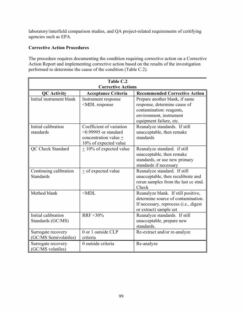
laboratory/interfield comparison studies, and QA project-related requirements of certifying agencies such as EPA. Corrective Action Procedures The procedure requires documenting the condition requiring corrective action on a Corrective Action Report and implementing corrective action based on the results of the investigation performed to determine the cause of the condition (Table C.2).

Table C.2 Corrective Actions

QC Activity Acceptance Criteria Recommended Corrective ActionInitial instrument blank Instrument response

<MDL response Prepare another blank, if same response, determine cause of contamination: reagents, environment, instrument equipment failure, etc.

Initial calibration standards

Coefficient of variation >0.99995 or standard concentration value + 10% of expected value

Reanalyze standards. If still unacceptable, then remake standards

QC Check Standard + 10% of expected value Reanalyze standard. if still unacceptable, then remake standards, or use new primary standards if necessary

Continuing calibration Standards

+ of expected value Reanalyze standard. If still unacceptable, then recalibrate and rerun samples from the last cc stnd. Check

Method blank <MDL Reanalyze blank. If still positive, determine source of contamination. If necessary, reprocess (i.e., digest or extract) sample set

Initial calibration Standards (GC/MS)

RRF <30% Reanalyze standards. If still unacceptable, prepare new standards.

Surrogate recovery (GC/MS Semivolatiles)

0 or 1 outside CLP criteria

Re-extract and/or re-analyze

Surrogate recovery (GC/MS volatiles)

0 outside criteria Re-analyze

99

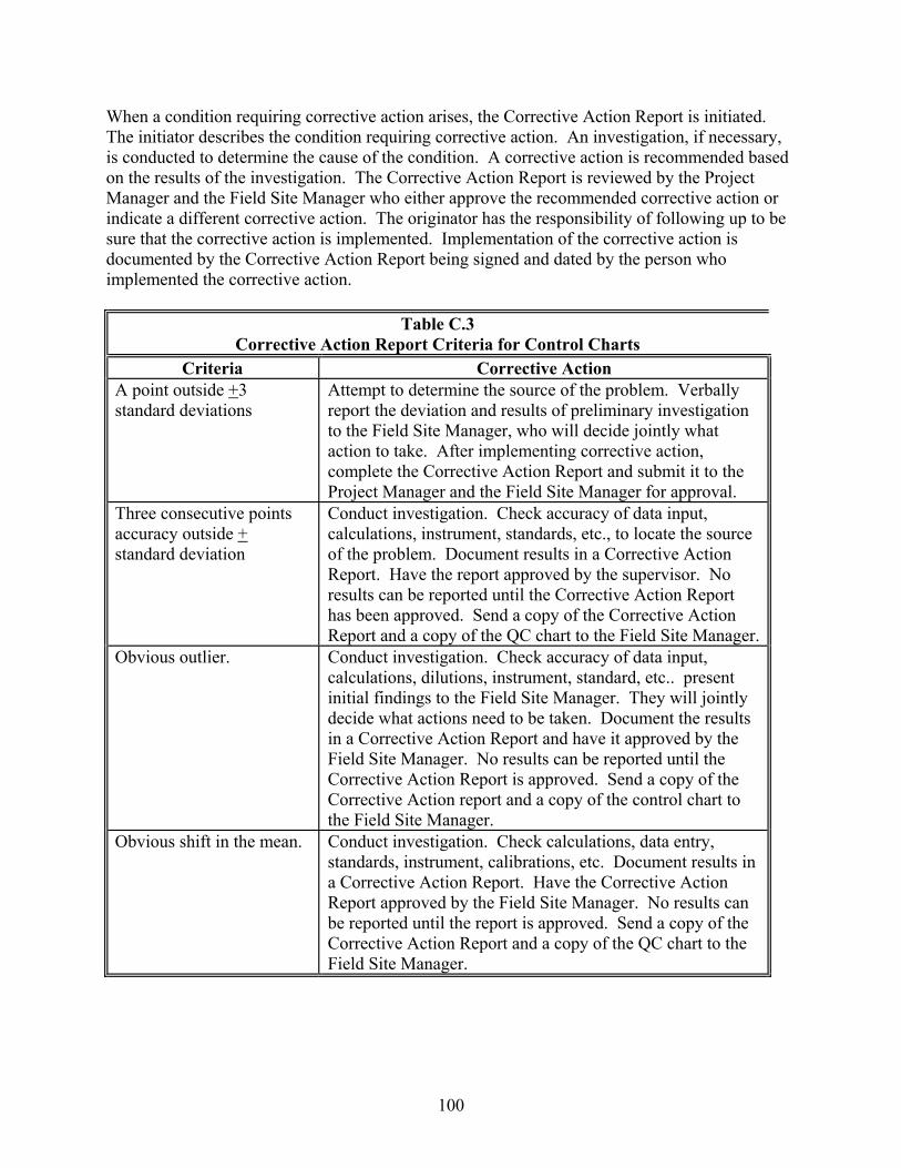
When a condition requiring corrective action arises, the Corrective Action Report is initiated. The initiator describes the condition requiring corrective action. An investigation, if necessary, is conducted to determine the cause of the condition. A corrective action is recommended based on the results of the investigation. The Corrective Action Report is reviewed by the Project Manager and the Field Site Manager who either approve the recommended corrective action or indicate a different corrective action. The originator has the responsibility of following up to be sure that the corrective action is implemented. Implementation of the corrective action is documented by the Corrective Action Report being signed and dated by the person who implemented the corrective action.

Table C.3 Corrective Action Report Criteria for Control Charts

Criteria Corrective Action A point outside +3 standard deviations

Attempt to determine the source of the problem. Verbally report the deviation and results of preliminary investigation to the Field Site Manager, who will decide jointly what action to take. After implementing corrective action, complete the Corrective Action Report and submit it to the Project Manager and the Field Site Manager for approval.

Three consecutive points accuracy outside + standard deviation

Conduct investigation. Check accuracy of data input, calculations, instrument, standards, etc., to locate the source of the problem. Document results in a Corrective Action Report. Have the report approved by the supervisor. No results can be reported until the Corrective Action Report has been approved. Send a copy of the Corrective Action Report and a copy of the QC chart to the Field Site Manager.

Obvious outlier. Conduct investigation. Check accuracy of data input, calculations, dilutions, instrument, standard, etc.. present initial findings to the Field Site Manager. They will jointly decide what actions need to be taken. Document the results in a Corrective Action Report and have it approved by the Field Site Manager. No results can be reported until the Corrective Action Report is approved. Send a copy of the Corrective Action report and a copy of the control chart to the Field Site Manager.

Obvious shift in the mean. Conduct investigation. Check calculations, data entry, standards, instrument, calibrations, etc. Document results in a Corrective Action Report. Have the Corrective Action Report approved by the Field Site Manager. No results can be reported until the report is approved. Send a copy of the Corrective Action Report and a copy of the QC chart to the Field Site Manager.

100

C.5 Demonstration Procedures Initiating the flux meter experiments will involve limited field effort. All of the components of the device can be prepared prior to field activities. In the field, the primary activity will be assembly of the flux meters which can be completed with two people in a mater of minutes. Extraction and sub-sampling also required fairly minimal time and personnel. Only the controlled flow flume experiments will require establishing steady flow from one end of the flume using peristaltic pumps. These pumps will be calibrated in the field using simple time and volume measurements. Periodic flow measurements will be made to determine total average flow. Samples collected at the Borden site will be sent to the University of Florida for analysis. In the laboratory, instrument maintenance will include the following. Maintenance Schedule Preventive maintenance, such as lubrication, source cleaning, and detector cleaning, is performed according to the procedures delineated in the manufacturer's instrument manuals. The frequency of preventive maintenance varies with different instruments. Routine maintenance performed includes cleaning and/or replacement of various instrument components. In general, the frequency recommended by the manufacturer is followed. In addition to the regular schedule, maintenance is performed as needed. Precision and accuracy data are examined for trends and excursions beyond control limits to determine evidence of instrument malfunction. Maintenance is performed when an instrument begins to degrade as evidenced by the degradation of peak resolution, shift in calibration curves, decreased ion sensitivity, or failure to meet one or another of the quality control criteria. Table E.4 lists routine equipment maintenance procedures and frequency. Instrument maintenance logbooks are maintained in the laboratory at all times. The logbook contains a complete history of past maintenance, both routine and nonroutine. The nature of work performed, the date, and the signature of the person who performed the work are recorded in the logbook. Preventive maintenance is scheduled according to each manufacturer's recommendation. Instrument downtime is minimized by keeping adequate supplies of all expendable items on hand. Expendable items are those with an expected lifetime of less than one year. Routine instrument preventive maintenance is handled by the instrument operator. Repair maintenance is performed by a full-time electronics technician, or by the manufacturer's service personnel.

101

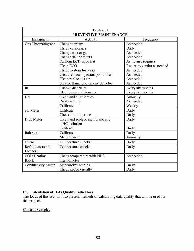
Table C.4

PREVENTIVE MAINTENANCE Instrument Activity Frequency

Gas Chromatograph Change septum Check carrier gas Change carrier gas Change in-line filters Perform ECD wipe test Clean ECO Check system for leaks Clean/replace injection point liner Clean/replace jet tip Service flame photomeric detector

As needed Daily As needed As needed As license requires Return to vendor as needed As needed As needed As needed As needed

IR Change desiccant Electronics maintenance

Every six months Every six months

UV Clean and align optics Replace lamp Calibrate

Annually As needed Weekly

pH Meter Calibrate Check fluid in probe

Daily Daily

D.O. Meter Clean and replace membrane and HCl solution Calibrate

Daily Daily

Balance Calibrate Maintenance

Daily Annually

Ovens Temperature checks Daily Refrigerators and Freezers

Temperature checks Daily

COD Heating Block

Check temperature with NBS thermometer

As needed

Conductivity Meter Standardize with KCl Check probe visually

Daily Daily

C.6 Calculation of Data Quality Indicators The focus of this section is to present methods of calculating data quality that will be used for this project. Control Samples

102

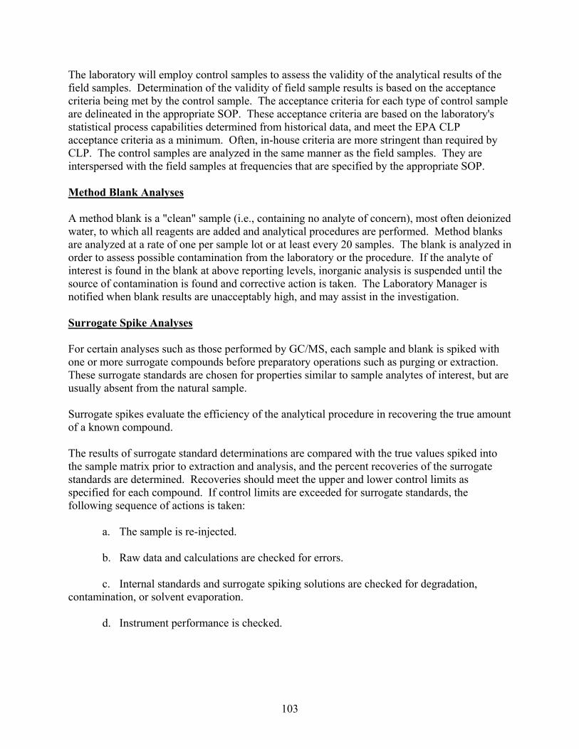
The laboratory will employ control samples to assess the validity of the analytical results of the field samples. Determination of the validity of field sample results is based on the acceptance criteria being met by the control sample. The acceptance criteria for each type of control sample are delineated in the appropriate SOP. These acceptance criteria are based on the laboratory's statistical process capabilities determined from historical data, and meet the EPA CLP acceptance criteria as a minimum. Often, in-house criteria are more stringent than required by CLP. The control samples are analyzed in the same manner as the field samples. They are interspersed with the field samples at frequencies that are specified by the appropriate SOP. Method Blank Analyses A method blank is a "clean" sample (i.e., containing no analyte of concern), most often deionized water, to which all reagents are added and analytical procedures are performed. Method blanks are analyzed at a rate of one per sample lot or at least every 20 samples. The blank is analyzed in order to assess possible contamination from the laboratory or the procedure. If the analyte of interest is found in the blank at above reporting levels, inorganic analysis is suspended until the source of contamination is found and corrective action is taken. The Laboratory Manager is notified when blank results are unacceptably high, and may assist in the investigation. Surrogate Spike Analyses For certain analyses such as those performed by GC/MS, each sample and blank is spiked with one or more surrogate compounds before preparatory operations such as purging or extraction. These surrogate standards are chosen for properties similar to sample analytes of interest, but are usually absent from the natural sample. Surrogate spikes evaluate the efficiency of the analytical procedure in recovering the true amount of a known compound. The results of surrogate standard determinations are compared with the true values spiked into the sample matrix prior to extraction and analysis, and the percent recoveries of the surrogate standards are determined. Recoveries should meet the upper and lower control limits as specified for each compound. If control limits are exceeded for surrogate standards, the following sequence of actions is taken: a. The sample is re-injected. b. Raw data and calculations are checked for errors. c. Internal standards and surrogate spiking solutions are checked for degradation, contamination, or solvent evaporation. d. Instrument performance is checked.

103

e. If a, b, and c fail to reveal the cause of the noncompliance surrogate recoveries, the sample is re-purged or re-extracted. f. If all the measures listed above fail to correct the problem for laboratory blank surrogate analyses, the analytical system is considered out of control, and the instrument must be recalibrated and examined for mechanical faults. g. If all the measures listed above fail to correct the problem for field sample surrogate analyses, the deficiency probably is due to sample interferences, and not due to any procedural or mechanical problems in the laboratory. The surrogate spike recovery data and the sample data from both extractions are reported and are flagged. The Laboratory Manager is notified with an exceptions report and the corrective actions taken. Matrix Spike/Matrix Spike Duplicate Analyses To evaluate the effect of the sample matrix on the analytical methodology, two separate aliquot samples may be spiked with a standard mix of compounds appropriate to a given analysis. The matrix spike and the matrix spike duplicate (MS/MSD) are analyzed at a frequency of one per lot or one per 20 samples, whichever is more frequent. The percent recovery for each of the spiking compounds is calculated. The relative percent difference (RPD) between the MS/MSD is also calculated. The observed percent recoveries (%R) and relative percent differences (RPD) between the MS/MSD are used to determine the accuracy and the precision of the analytical method for the sample matrix. If the percent recovery and RPD results exceed the control limits as specified for each spiking compound, the sample is not reanalyzed. Poor recovery in matrix spiked samples does not necessarily represent an analytical system out of control. It is possible that unavoidable interferences and matrix effects from the sample itself preclude efficient recoveries. The poor recovery is documented for the Project Manager. Internal Standards Analysis Once an instrument has been calibrated, it is necessary to confirm periodically that the analytical system remains in calibration. The continuing calibration and precision of the organics analytical system are checked for each sample analysis by monitoring the instrument response to internal standards. When internal standard addition is not appropriate to a particular method, other means of accuracy checks, such as standard addition, are used. Results from internal standard analyses are compared to the mean calibrated value. Deviation from this mean beyond a predetermined magnitude, depending on the type of analysis, defines an out-of-control condition. The system must then be brought back into control by: • Checking the quality of the internal standards and reanalyzing the sample

104

• Recalibrating the system • Correcting the malfunctions causing the instrument to fall out of calibration Duplicate Sample Analyses Duplicate analyses are performed for cations analyses and upon special request for selected other parameters to evaluate the reproducibility of the method. Results of the duplicate analyses are used to determine the RPD between replicate samples. For each parameter analyzed, at least one duplicate sample is run per group of 20 samples. The precision value, RPD, is reviewed by the section supervisor and the division manager. If the precision value exceeds the control limit or the established protocol criteria for the given parameter, the sample set is reanalyzed for the parameter in question unless it is determined that heterogeneity of the sample has caused the high RPD. QC Check Standard Analyses Analysis of QC check standards is used to verify the preparation process or the standard curve, and is performed with each group of samples. Results of these data are summarized, evaluated, and presented to the section supervisor and the division manager for review. The results of the QC check standard analysis are compared with the true values, and the percent recovery of the check standard is calculated. If correction of a procedure or instrument repair is done, the check standard is reanalyzed to demonstrate that the corrective action has been successful. At least twice a year, a QC check standard for each parameter group is analyzed as a double-blind sample. Samples are prepared, submitted, and evaluated by the Laboratory Manager. Other Quality Control Samples Under some sampling analysis, additional quality control samples may be required. These may include: a. Blank/Spike--Analyte of interest or surrogate is spiked into blank water rather than into a sample. The blank/spike goes through the entire analytical procedure, and percent recovery is calculated with no likelihood of matrix effect. For many contracts, an externally provided LCS sample (EPA) serves as a blank/spike sample. b. Trip Blank--A sample bottle filled with laboratory blank water travels with the sample kit to the sampling site, and is sent back to the laboratory packed in the same container as

105

any volatile samples collected. Trip blank analyses check for possible volatile contamination during shipping or sampling. c. Field Blank--A field blank can be a sample container filled with laboratory blank water and sent to the sampling site, or it may be filled at the site with purchased distilled water or decontamination water. The field blank analysis checks for possible contamination by the sampling team. d. Equipment Rinsates--After equipment has been cleaned in the field, many contracts require that the equipment be rinsed and the rinsate analyzed for the same parameters requested on the samples. The rinsate analysis proves the equipment has been cleaned properly and will not contaminate the next samples taken. Control Charts The laboratory will use control charts to monitor for out-of-control conditions. Control Charting Process The control chart program uses a series of Lotus (or equivalent) macros to perform data processing and control charting. These macros also perform statistical decisions on the acceptability of the data. The control chart used is a variation of the Shewart control chart of averages. The chart plots individual quantitative results against the order of time measurement. The plotted values are compared with control limits determined by the variability about the mean of the standard "in control" process. The control chart estimates the process mean and the variability from a moving window of 50 to 200 samples, depending upon the analytical parameters involved. The mean is estimated from the arithmetic average of the samples in the current window. The variability is estimated as the sample SD of the sample values in the current window. The program calculates the 2 SD and the 3 SD limits and displays them on the chart. The t-statistic is used to estimate the 99.7 percent tolerance limits for the degrees of freedom in the current window. Values outside the t-statistic limits are unconditionally rejected from inclusion in the sample window and automatically documented in a Corrective Action Report (CAR). The CAR prompts the analyst to initiate investigation and corrective action. When the maximum number of samples has accumulated in the current window, the summary statistics of the mean and SD are written to the long-term data base. The last 20 samples in the old window are then transferred to a new window for continued use in the charting process. The long-term data base charts the mean 1 SD error bars.

106

Instrument Detection Limits, Method Detection Limits, and Reporting Limits Instrument Detection Limits (IDL) Instrument Detection Limit (IDL) studies are performed for inorganic parameters when an instrument is installed, when major maintenance or repair work has been done, and routinely once per calendar quarter. To determine IDL, seven consecutive measurements per day are made on a prepared standard solution (in reagent water) of an analyte at a concentration 3 to 5 times the instrument manufacturer's suggested IDL. Each measurement is performed as though it were a separate analytical sample. This procedure is repeated on three nonconsecutive days. The standard deviation is calculated for each set of seven replicates and the average of the standard deviations is obtained. This average is multiplied by 3 to give the instrument detection limit (IDL). Method Detection Limits (MDL) The Method Detection Limit (MDL) is the minimum concentration of a substance that can be measured and reported with 99 percent confidence that the value is above zero. The sample must be carried through the entire method under ideal conditions. MDL is determined according to the method outlined in 40 CFR 136, Appendix B. MDLs are determined at least annually for all parameters. MDL studies are also conducted for new methods introduced in the lab, after major maintenance or modification to an instrument, and as part of the training of new analysts. To determine MDL, seven replicate analyses are made of analytes spiked into blank water at 1 to 5 times the estimated method detection limit. The spiked samples must be carried through the entire analytical procedure, including any extraction, digestion, or distillation process, for MDL calculation. The SD of these replicates is calculated. Where: t = The student t value for a 99% confidence interval

Sx t = MDL

S = Standard deviation of the replicate analyses Reporting Limits In most cases, final report forms list reporting limits rather than either IDL or MDL. Reporting limits are taken from EPA SW846 published limits or from historical data. Matrixes or analyte concentrations which require dilution will change the detection limits for that sample. C.7 Performance and System Audits In this section information is provided on performance audits and onsite system audits.

107

Performance Evaluation Samples Performance evaluation samples are analyzed throughout the project for all parameters, as a constant check on accuracy and precision for all analyses. Audits Internal audits of the laboratory are conducted in two phases. The first phase is conducted by the Laboratory Quality Assurance Coordinator during the fourth quarter of the year. This is usually a 2-day systems audit which covers all sections of the laboratory. An audit report is issued within 2 weeks of completion. The Field Site Manager has the responsibility for coordinating all responses to the audit finding and for following up on the required corrective action. A followup audit is made when deemed necessary by the by the Field Site Manager or the Laboratory Manager. A quality assurance review questionnaire is provided in the Appendix. The second phase consists of quarterly audits performed by the Field Site Manager. These are half-day or day-long audits, and are concentrated on specific areas that are deemed problem areas by the Field Site Manager. An audit report is issued at the completion of the audit. Responses and followup corrective action to the audit findings are required, and are monitored by the Field Site Manager. All audit reports are issued to management and circulated to all staff. Copies are filed with the Field Site Manager and the Laboratory Manager. C.8 Quality Assurance Reports The performance of the field laboratory as assessed by the quality monitoring systems in place is reported by the Field Site Manager to management quarterly and as needed. Copies of all quality reports are maintained in the Field Site Manager and Laboratory Manager files. Quality assurance reports to management include, but are not limited to, the following: • Results of performance and systems audits • Status of corrective actions • Periodic assessment of data accuracy, precision, and completeness • Significant QA problems and recommended solutions In addition to the quarterly reports, a final report summarizing items covered in the quarterly reports is provided by the Field Site Manager to the Project Manager. C.9 Data Format

108

Introduction In order to provide analytical data which is technically sound and defensible, a system of data management will be implemented in the laboratory. All activities which pertain to a sample are documented. All data generated during the demonstration, except those that are generated by automated data collection systems, will be recorded directly, promptly, and legibly in ink. All data entries will be dated on the day of entry and signed or initialed by the person entering the data. Any change in entries will not obscure the original entry, will indicate the reason for such change, and will be dated and signed or identified at the time of the change. In automated data collection systems, the individual responsible for direct data input will be identified at the time of data input. Any change in automated data entries will not obscure the original entry. Updated entries will indicate the reason for the change, the date, and the person responsible for making the change. Data Tracking in the Laboratory The Field Site Manager is responsible for developing a system for tracking and maintaining sample identity between the collection point, analysis and reporting. This process will be periodically reviewed by the Project Manager. Analyses and Data Reduction The Field Site Manager is responsible for the reduction of raw data when such steps are required to produce the correct data format for reporting. Data reduction may be done manually or through one of a number of computer programs used in the laboratory. Chromatogram Identification In the GC section computer software is used to identify chromatograms. A system-supplied file name (a hexadecimal date-time) and a user-supplied file name (related to an entry in the injection log) identify each acquisition. Data Reduction Formulas Linear regression formulas are used in a computer software system to calculate samples values for many general inorganic parameters and metals analyses. These programs use the general formula for linear regression:

bx +a = Y ′

109

where: Y' = The predicted value of y for a selected value of x a = The value of y when x = 0 b = The slope of the straight line x = Any value of x selected Sample values for GC/MS parameters are calculated by systems software using the general formula:

Factor Response x Area

Amount x AreaIS

IS

Target

GC data is calculated using either an internal or an external standard. For internal standards:

( ) ⎟⎠

⎞⎜⎝

⎛⎟⎠⎞

⎜⎝⎛⎟

⎠

⎞⎜⎝

⎛⎟⎠

⎞⎜⎝

⎛Amtamt

TP amt

AA

AA = ionConcentrat

standardIS

SampleISstandard

xsampleIS

standardIS

standardx

samplex

where: P = 1/fraction of extract to which IS is added For calculations using an external standard:

( ) ⎟⎠⎞

⎜⎝⎛⎟

⎠

⎞⎜⎝

⎛TV C

AA = ionConcentrat standard

xstandardx

samplex

where: C = concentration of x in standard V = volume of final extract T = total sample extracted C.10 Data Storage and Archiving Procedures Data from GC's will be saved and archived in P&E Turbochrom format. All data will be backed-up on ZIP disks. This data will be batch processed into an Excel .csv file that can be easily converted to an Excel Worksheet. These files will be backed-up and transferred to individuals responsible for calculating flux results. All data related to the project will be organized for rapid retrieval and transfer to other interested parties.

110

Appendix D: Health and Safety Plan

111

Field Evaluation of the Florida Flux Meter at Canadian Forces Base Borden, Ontario

Health and Safety Plan

May 15, 2007

University of Florida, Gainesville, FL

TABLE OF CONTENTS

SECTION PAGE Introduction 1 1.0 Site Description, Investigation Activities, and Hazard Summaries 1 1.1 Site Background 1 1.2 Field Activities 1 1.3 Site Hazard Evaluation 1 1.4 Activity Hazard Analysis 4 2.0 Assignment of Responsibilities 5 2.1 Project Manager 5 2.2 Project Safety Officer 5 2.3 Field Team Leader/Site Safety Officer 6 2.4 Field Staff 6 3.0 Personnel Training 8 4.0 Personal Protective Equipment 11 4.1 Level D Personal Protective Equipment 11 4.2 Level C Personal Protective Equipment 11 4.3 Respirator Selection and Fit Test 11 5.0 Hazard Assessment 12 5.1 Site Area Survey 12 5.2 Air Monitoring 12 5.3 Cold Stress Monitoring 12 6.0 Site Control 13 6.1 Regulated Areas 13 6.2 Work Zones 13 7.0 Decontamination Procedures 14 7.1 Decontamination of Personnel 14 7.2 Equipment Decontamination and Disposal of 15 Contaminated Materials 8.0 General Site Safety Requirements 15 9.0 Emergency Procedures 16 9.1 Accident Prevention and Hazard Analysis 16 9.2 Emergency Medical Assistance and First Aid Equipment 18 9.3 Emergency Protocol 18 9.4 Decontamination During Medical Emergencies 19 10.0 Chemical Hazards and Control 22 10.1 Flammable Materials Storage and Handling 22 10.2 Fire Protection Plan 24

i

LIST OF TABLES

TABLE PAGE 1 Site Hazard Summary 3 2 Safety and Emergency Equipment 17 3 Emergency Assistance Information 20

LIST OF FIGURES

FIGURE PAGE 1 Site Safety Responsibility Chart 7 2 Personal Acknowledgment 9 3 Site Safety Meeting Form 10 4 Hospital Route Map 21

ii

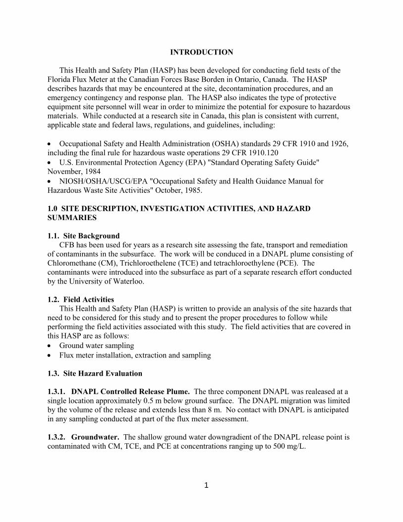
INTRODUCTION This Health and Safety Plan (HASP) has been developed for conducting field tests of the Florida Flux Meter at the Canadian Forces Base Borden in Ontario, Canada. The HASP describes hazards that may be encountered at the site, decontamination procedures, and an emergency contingency and response plan. The HASP also indicates the type of protective equipment site personnel will wear in order to minimize the potential for exposure to hazardous materials. While conducted at a research site in Canada, this plan is consistent with current, applicable state and federal laws, regulations, and guidelines, including: • Occupational Safety and Health Administration (OSHA) standards 29 CFR 1910 and 1926, including the final rule for hazardous waste operations 29 CFR 1910.120 • U.S. Environmental Protection Agency (EPA) "Standard Operating Safety Guide" November, 1984 • NIOSH/OSHA/USCG/EPA "Occupational Safety and Health Guidance Manual for Hazardous Waste Site Activities" October, 1985. 1.0 SITE DESCRIPTION, INVESTIGATION ACTIVITIES, AND HAZARD SUMMARIES 1.1. Site Background CFB has been used for years as a research site assessing the fate, transport and remediation of contaminants in the subsurface. The work will be conduced in a DNAPL plume consisting of Chloromethane (CM), Trichloroethelene (TCE) and tetrachloroethylene (PCE). The contaminants were introduced into the subsurface as part of a separate research effort conducted by the University of Waterloo. 1.2. Field Activities This Health and Safety Plan (HASP) is written to provide an analysis of the site hazards that need to be considered for this study and to present the proper procedures to follow while performing the field activities associated with this study. The field activities that are covered in this HASP are as follows: • Ground water sampling • Flux meter installation, extraction and sampling 1.3. Site Hazard Evaluation 1.3.1. DNAPL Controlled Release Plume. The three component DNAPL was realeased at a single location approximately 0.5 m below ground surface. The DNAPL migration was limited by the volume of the release and extends less than 8 m. No contact with DNAPL is anticipated in any sampling conducted at part of the flux meter assessment. 1.3.2. Groundwater. The shallow ground water downgradient of the DNAPL release point is contaminated with CM, TCE, and PCE at concentrations ranging up to 500 mg/L.

1

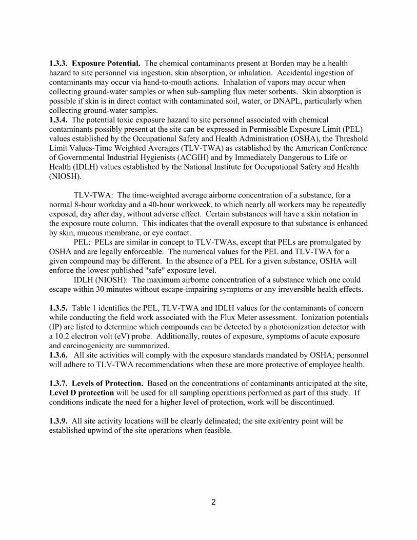
1.3.3. Exposure Potential. The chemical contaminants present at Borden may be a health hazard to site personnel via ingestion, skin absorption, or inhalation. Accidental ingestion of contaminants may occur via hand-to-mouth actions. Inhalation of vapors may occur when collecting ground-water samples or when sub-sampling flux meter sorbents. Skin absorption is possible if skin is in direct contact with contaminated soil, water, or DNAPL, particularly when collecting ground-water samples. 1.3.4. The potential toxic exposure hazard to site personnel associated with chemical contaminants possibly present at the site can be expressed in Permissible Exposure Limit (PEL) values established by the Occupational Safety and Health Administration (OSHA), the Threshold Limit Values-Time Weighted Averages (TLV-TWA) as established by the American Conference of Governmental Industrial Hygienists (ACGIH) and by Immediately Dangerous to Life or Health (IDLH) values established by the National Institute for Occupational Safety and Health (NIOSH). TLV-TWA: The time-weighted average airborne concentration of a substance, for a normal 8-hour workday and a 40-hour workweek, to which nearly all workers may be repeatedly exposed, day after day, without adverse effect. Certain substances will have a skin notation in the exposure route column. This indicates that the overall exposure to that substance is enhanced by skin, mucous membrane, or eye contact. PEL: PELs are similar in concept to TLV-TWAs, except that PELs are promulgated by OSHA and are legally enforceable. The numerical values for the PEL and TLV-TWA for a given compound may be different. In the absence of a PEL for a given substance, OSHA will enforce the lowest published "safe" exposure level. IDLH (NIOSH): The maximum airborne concentration of a substance which one could escape within 30 minutes without escape-impairing symptoms or any irreversible health effects. 1.3.5. Table 1 identifies the PEL, TLV-TWA and IDLH values for the contaminants of concern while conducting the field work associated with the Flux Meter assessment. Ionization potentials (IP) are listed to determine which compounds can be detected by a photoionization detector with a 10.2 electron volt (eV) probe. Additionally, routes of exposure, symptoms of acute exposure and carcinogenicity are summarized. 1.3.6. All site activities will comply with the exposure standards mandated by OSHA; personnel will adhere to TLV-TWA recommendations when these are more protective of employee health. 1.3.7. Levels of Protection. Based on the concentrations of contaminants anticipated at the site, Level D protection will be used for all sampling operations performed as part of this study. If conditions indicate the need for a higher level of protection, work will be discontinued. 1.3.9. All site activity locations will be clearly delineated; the site exit/entry point will be established upwind of the site operations when feasible.

2

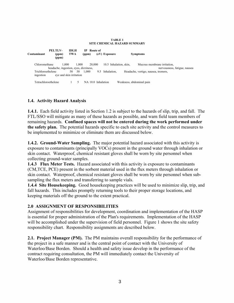
TABLE 1 SITE CHEMICAL HAZARD SUMMARY PEL TLV- IDLH IP Route of Contaminant (ppm) TWA (ppm) (eV) Exposure Symptoms (ppm) Chloromethane 1,000 1,000 20,000 10.5 Inhalation, skin, Mucous membrane irritation, headache, ingestion, eyes, dizziness, nervousness, fatigue, nausea Trichloroethelene 50 50 1,000 9.5 Inhalation, Headache, vertigo, nausea, tremors, ingestion eye and skin irritation Tetrachloroethelene 1 5 NA 10.0 Inhalation Weakness, abdominal pain 1.4. Activity Hazard Analysis 1.4.1. Each field activity listed in Section 1.2 is subject to the hazards of slip, trip, and fall. The FTL/SSO will mitigate as many of these hazards as possible, and warn field team members of remaining hazards. Confined spaces will not be entered during the work performed under the safety plan. The potential hazards specific to each site activity and the control measures to be implemented to minimize or eliminate them are discussed below. 1.4.2. Ground-Water Sampling. The major potential hazard associated with this activity is exposure to contaminants (principally VOCs) present in the ground water through inhalation or skin contact. Waterproof, chemical resistant gloves shall be worn by site personnel when collecting ground-water samples. 1.4.3 Flux Meter Tests. Hazard associated with this activity is exposure to contaminants (CM,TCE, PCE) present in the sorbent material used in the flux meters through inhalation or skin contact. Waterproof, chemical resistant gloves shall be worn by site personnel when sub-sampling the flux meters and transferring to sample vials. 1.4.4 Site Housekeeping. Good housekeeping practices will be used to minimize slip, trip, and fall hazards. This includes promptly returning tools to their proper storage locations, and keeping materials off the ground to the extent practical. 2.0 ASSIGNMENT OF RESPONSIBILITIES Assignment of responsibilities for development, coordination and implementation of the HASP is essential for proper administration of the Plan's requirements. Implementation of the HASP will be accomplished under the supervision of field personnel. Figure 1 shows the site safety responsibility chart. Responsibility assignments are described below. 2.1. Project Manager (PM). The PM maintains overall responsibility for the performance of the project in a safe manner and is the central point of contact with the University of Waterloo/Base Borden. Should a health and safety issue develop in the performance of the contract requiring consultation, the PM will immediately contact the University of Waterloo/Base Borden representative.

3

2.2. Project Safety Officer (PSO). The PSO is responsible for the preparation of the site-specific HASP. The PSO will ensure that the safety plan complies with all federal, state and local health and safety requirements. If necessary, the PSO can modify the site-specific HASP to adjust for on site changes that affect safety. The Field Team Leader/Site Safety Officer cannot modify the HASP without the approval of the PSO in order to avoid conflicts between meeting program deadlines and safety issues. The PSO will prepare the materials to be used in the training program and insure that the Site Safety Officer is knowledgeable of all components of the HASP. 2.3. Field Team Leader/Site Safety Officer (FTL/SSO). The FTL/SSO is responsible for the implementation of the HASP and has the responsibility and authority to halt or modify any working condition, or remove personnel from the site if he considers conditions to be unsafe. The FTL/SSO will be the main contact in any on-site emergency situation, and will direct all field activities involved with safety. The FTL/SSO is responsible for assuring that all on-site personnel understand and comply with all safety requirements. Except in an emergency, the FTL/SSO can modify the HASP requirements only after consultation with and agreement of the PSO. The FTL/SSO will conduct an initial safety meeting with all on site personnel prior to beginning the field experiments. Additional safety meetings will be conducted when new personnel arrive and when site health and safety conditions change. In the meetings, the potential hazards that the workers may encounter while performing the field work will be discussed. 2.4. Field Staff. All field staff, including subcontractor personnel, are responsible for understanding and complying with all requirements of the HASP. Field staff will be instructed to bring all perceived unsafe site conditions to the attention of the FTL/SSO.

4

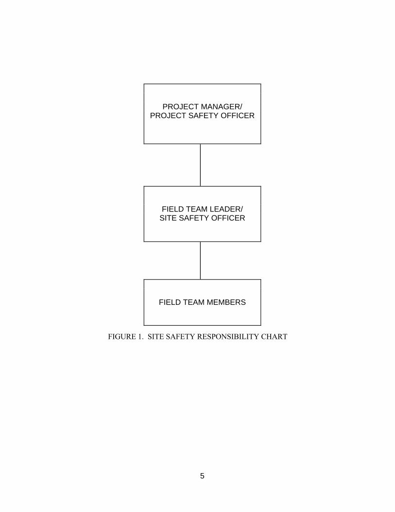
PROJECT MANAGER/

PROJECT SAFETY OFFICER

FIELD TEAM LEADER/ SITE SAFETY OFFICER

FIELD TEAM MEMBERS

FIGURE 1. SITE SAFETY RESPONSIBILITY CHART

5

3.0 PERSONNEL TRAINING 3.0.1. The FTL/SSO shall ensure that all personnel have received the required training for those tasks they are assigned to perform, prior to working on-site. 3.0.2. The FTL/SSO shall maintain a file of completed personal acknowledgments (Figure 2). Each site worker must sign and date this document acknowledging that he or she has read, understood, and intends to comply with the HASP. Copies of completed personal acknowledgments will be submitted to the client or the authorized representative on request. 3.0.3. As discussed in section 2.3, the FTL/SSO must conduct a site safety meeting before the experiment begins, whenever new personnel arrive at the site, and as site conditions change. A brief daily safety meeting will be conducted to address such issues as the types of accidents most likely to occur and areas where improvements need to be made with respect to health and safety. Potential topics of discussion at all sessions include: • Protective Clothing/Equipment • Chemical Hazards • Physical Hazards • Emergency Procedures • Hospital/Ambulance Route • Standard Operating Procedures • Other safety topics which are relevant to the site A site safety meeting form will be completed and signed at the end of the kickoff safety meeting. A sample site safety meeting form is presented in Figure 3.

6

As a component of the Health and Safety Plan (HASP) designed to provide personnel safety during the Field Evaluation of Cosolvent Enhanced Remediation field activities at Hill AFB Operable Unit 1 site in Layton, Utah, you are required to read and understand the HASP. When you have fulfilled this requirement, please sign and date this personal acknowledgment. Signature Date Name (Printed) FIGURE 2. PERSONAL ACKNOWLEDGMENT

7

Date: Time: Client: University of Waterloo Site Location: CFB Borden, Ontario, Canada Scope of Work:

SAFETY TOPICS PRESENTED Protective Clothing/Equipment: Chemical Hazards: Physical Hazards: Special Equipment: Other: Emergency Procedures: Hospital: Phone: Ambulance Phone: Hospital Address and Route:

ATTENDEES NAME PRINTEDSIGNATURE

Meeting Conducted By: Project Manager/Project Safety Officer:

FIGURE 3. SITE SAFETY MEETING FORM

3.0.4. Part of personnel training is to know standard and emergency procedures. These procedures are specified in Sections 9 and 10. A hospital route map is shown in Figure 4. All personnel should be familiar with the route to the hospital.

8

4.0 PERSONAL PROTECTIVE EQUIPMENT 4.0.1. Personal protective equipment (PPE) will be required during the course of the field work at Borden. PPE selection will be based primarily on hazard assessment data and work task requirements. 4.0.2. Based on the known contaminant release, the level of protection for all field activities is Level D. The personal protective equipment associated with Level D is described below. 4.1. Level D Personal Protective Equipment 4.1.1. Personnel working in an exclusion zone, which is defined in Section 8.1, shall wear as a minimum: • Work uniform - during ground-water sampling, if there is limited potential for contaminated ground water to splash onto site personnel. • Gloves, chemical-resistant (nitrile) - Chemical resistant gloves required for ground-water sampling. • Safety glasses - Eye protection required if there is a potential for injection fluids or contaminated ground water to splash onto site personnel. 5.0 HAZARD ASSESSMENT 5.0.1. Hazard assessment is essential for determination of hazard control measures that must be implemented during site activities; it involves characterization of the chemical, physical and other safety hazards at the site. Hazard assessment is an on-going process. 5.1. Site Area Survey 5.1.1. The FTL/SSO shall conduct a site survey at each work area to locate hazards and to determine appropriate control measures prior to initiation of work activities. Hazards may include obstacles to ground traffic and slip/trip and fall hazards. 5.2. Cold Stress Monitoring 5.2.1. Because the field work will probably be conducted in summer and fall, there is a potential for either frostbite or hypothermia to occur. The following paragraphs describe these phenomena and measures that should be taken to prevent them from occurring. 5.2.2. Hypothermia. Hypothermia is defined as a decrease of the body core temperature below 96F. Symptoms of hypothermia include shivering, apathy, listlessness, sleepiness, and unconsciousness. Hypothermia can occur at temperatures as high as 40oF, especially if it is raining.

9

5.2.3. Frostbite. Frostbite refers to areas of local cold injury. Symptoms of frostbite include whitening of the skin, skin that has a waxy or white appearance and is firm to the touch, and tissues that are cold, pale, and solid. Unlike hypothermia, frostbite rarely occurs unless the temperature is below freezing, and normally temperatures must be less than 20oF. 5.2.4. Prevention of Cold Related Illnesses. When there is a significant potential for cold stress, the following measures should be taken: • Educate workers to recognize the symptoms of frostbite and hypothermia. • Ensure that workers wear clothing that will keep them warm and dry. • Take breaks in a heated area as necessary to allow workers to warm up. Hot liquids should be available in this area. 6.0 SITE CONTROL 6.0.1. Site control requires the establishment of a regulated area, designated work zones, an evacuation protocol, and site security. 6.1. Regulated Area(s) 6.1.1. To minimize the potential transfer of and exposure to potentially hazardous substances, contamination control procedures are necessary. Two general methods will be used: establishing site work zones (Exclusion, Contamination Reduction, Support) and personnel/equipment decontamination. The site must be controlled to reduce the possibility of: 1) exposure to any contaminants present, and 2) their transport by personnel or equipment from the site. The possibility of exposure or translocation of substances will be reduced or eliminated in a number of ways, including: Setting up physical barriers to exclude unnecessary personnel from the work areas Minimizing the number of personnel on site consistent with efficient operations Establishing work zones around the ground-water sampling area and storage tank area Establishing control points to regulate access to work zones Implementing appropriate decontamination procedures. 6.1.2. Safety procedures for preventing or reducing the migration of contamination require the delineation of zones in the work areas on the site where prescribed operations occur. Movement of personnel and equipment between zones and onto the site itself will be limited by access control points. The site will be outlined with survey tape or other appropriate means to define the work areas and to identify the entry and exit points. 6.1.3. Personnel on site will use the "buddy system" and will maintain communication or visual contact between team members at all times in the designated work zones where ground-water sampling and storage tank operations occur. 6.2. Work Zones

10

6.2.1. All work areas requiring PPE will have the following zones established: Zone 1: Exclusion Zone (work zone in which prescribed PPE will be maintained) Zone 2: Contamination Reduction Zone/Corridor Zone 3: Support Zone (no PPE required) 6.2.2. Zone 1: Exclusion Zone (work zone). The exclusion zone, the innermost of the three designated areas, will be the area where activities require personnel protective equipment (PPE). All personnel entering the exclusion zone must wear the prescribed PPE. An entry and exit check point must be established at the periphery of the exclusion zone to regulate the flow of personnel and equipment into and out of the zone. The outer boundary of the exclusion zone, the "hotline", will be established by visually surveying the site and determining the area where significant amounts of organic vapors and/or a potential for explosive vapor conditions might exist. Physical hazards associated with the work task will be identified in the exclusion zones. Once the "hotline" has been determined, it will be defined by the use of stakes, cones, or surveyor tape. During subsequent site operations, the boundary may be modified and adjusted by the FTL/SSO as more information becomes available. Potential exclusion zones at the Borden site have been identified as the ground water sampling sites. 6.2.3. Personnel will be decontaminated as they move through the contamination reduction corridor. Detailed decontamination procedures are provided in Section 7. 6.2.4. Zone 3: Support Zone. The support zone, the outermost part of the site, will be considered a noncontaminated or clean area. Support equipment (command post/trailer, safety vehicle, etc.) is located in this area. 6.2.6. The location of the command post and other support facilities in the support zone at each site depends on a number of factors, including: • Accessibility: topography; open space available; locations of roads; or other limitations • Wind direction: preferably the support facilities should be located upwind of the exclusion zone. Shifts in wind direction and other conditions may be such that an ideal location based on wind direction alone does not exist • Resources: water, electrical power. 6.2.7. Access to the contamination reduction corridor from the support zone is through a controlled access point. Personnel entering the contamination reduction corridor to assist in decontamination must wear the prescribed personal protective equipment. Reentry into the support zone requires removal of any protective equipment worn in the contamination reduction corridor. 7.0 DECONTAMINATION PROCEDURES 7.0.1. Establishment of decontamination procedures for personnel and equipment are necessary to control contamination and to protect field personnel.

11

7.1. Decontamination of Personnel 7.1.1. Personnel will be decontaminated upon leaving the exclusion zone to the appropriate extent as directed by the FTL/SSO based upon organic vapors generated or gross visual contamination of protective clothing. When complete decontamination is required, it will consist of the following: • At the "hotline" of the contamination reduction corridor, personnel will deposit equipment used on site, such as tools, sampling devices and containers, monitoring instruments, and clipboards. • If being worn, chemical resistant gloves and coveralls or apron will be disposed of at the “hotline”. • Ground-water sampling equipment will be cleaned in a solution of detergent and water, followed by multiple rinsings with water. • PPE will be removed in the following order: disposable coveralls or apron, respirator, and gloves. 7.1.2. Personnel shall be instructed in the proper decontamination technique, which entails removal of protective clothing in an "inside-out" manner. Removal of contaminants from clothing or equipment by blowing, shaking or any other means that may disperse material into the air is prohibited. 7.1.3. All disposable personal protective clothing that has been removed will be containerized at the decontamination station pending disposal. At the conclusion of work in a site exclusion zone, all protective equipment must be placed in plastic bags prior to disposal or transfer off-site. Non-disposable equipment will be decontaminated and properly stored outside the exclusion zone when not in use. 7.1.4. All employees will wash their hands and face with soap and water or disinfectant moist towelettes before eating, drinking, smoking, or applying cosmetics. These activities will be restricted to the designated rest area(s) in the support zone. This restriction also applies to work activities that do not require an exclusion zone, such as ground-water sampling. 7.2. Equipment Decontamination and Disposal of Contaminated Materials 7.2.1. Equipment that may require decontamination includes water sampling devices and certain protective equipment. 7.2.2. All materials and equipment used for decontamination must be disposed of properly. Disposable clothing, tools, buckets, brushes, and all other equipment that is contaminated will be secured in appropriate Department of Transportation (DOT) specification 55-gallon drums or other containers and marked. Clothing that will be reused, but which is not completely decontaminated on site, will be secured in plastic bags before being removed from the site. Contaminated wash water solutions shall be transferred to the effluent storage tank, pending transfer to a specified location for subsequent treatment. 8.0 GENERAL SITE SAFETY REQUIREMENTS

12

8.0.1. The following practices are expressly forbidden during on-site investigations: • Smoking, eating, drinking, or chewing gum or tobacco while in the work zone or any potentially contaminated area. • Ignition of flammable materials in the work zone; equipment shall be bonded and grounded, spark-proof and explosion resistant, as appropriate. • Contact with potentially contaminated substances. Walking through puddles or pools of liquid, kneeling on the ground or leaning, sitting or placing equipment on contaminated soil should be avoided. • Performance of tasks in the exclusion zone individually, except for those tasks explicitly permitted by the HASP. 8.0.2. Equipment to be maintained on site is listed in Table 2. Posted at the site will be the hospital route map (Figure 4). Personnel should keep the following rules in mind when conducting an on-site investigation: • Hazard assessment is a continual process; personnel must be aware of their surroundings and constantly be aware of the chemical/physical hazards that are present. • Personnel in the exclusion zone shall be the minimum number necessary to perform work tasks in a safe and efficient manner. • Team members will be familiar with the physical characteristics of each investigation site, including wind direction, site access, location of communication devices, and safety equipment. 9.0 EMERGENCY PROCEDURES 9.1. Accident Prevention and Hazard Analysis 9.1.1. The prevention of injuries and the minimization of risks are the responsibility of all site workers. Specific procedures to both prevent accidents and to handle them should they occur are presented in this section.

13

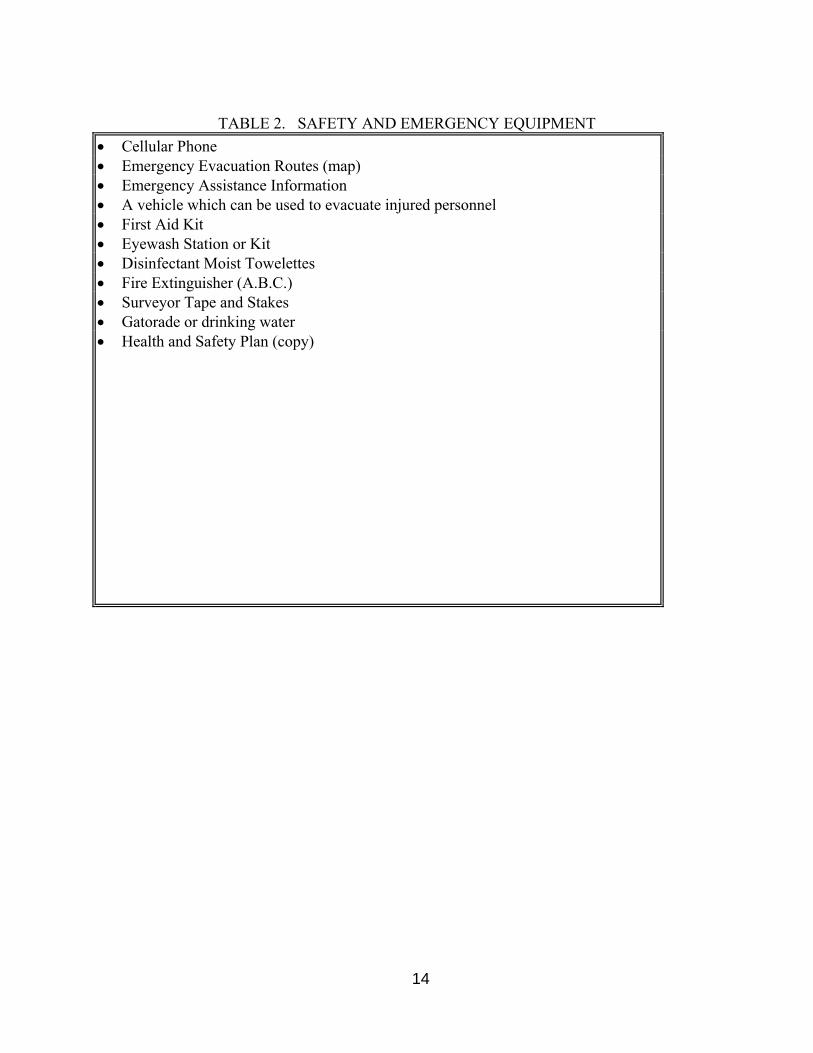
TABLE 2. SAFETY AND EMERGENCY EQUIPMENT

• Cellular Phone • Emergency Evacuation Routes (map) • Emergency Assistance Information • A vehicle which can be used to evacuate injured personnel • First Aid Kit • Eyewash Station or Kit • Disinfectant Moist Towelettes • Fire Extinguisher (A.B.C.) • Surveyor Tape and Stakes • Gatorade or drinking water • Health and Safety Plan (copy)

14

9.1.2. The Field Team Leader/Site Safety Officer will be responsible for implementation of this accident prevention plan and all on-site personnel will be accountable for reading, understanding and following the guidelines contained herein. • An initial indoctrination of all site personnel, and site-specific safety training, will be accomplished during the training session described in Section 3. • The Field Team Leader/Site Safety Officer will be responsible for maintaining a clean job site, free from hazards, and providing safe access and egress from the site. Cones and high visibility surveyor tape will be utilized for traffic control, and limiting access to hazardous and restricted areas. • Emergency phone numbers will be posted for the Fire Department and the nearest emergency medical clinic/hospital. The fastest route to the clinic/hospital, along with emergency telephone numbers, are found in Table 3. The FTL/SSO will be the lead person in all emergency situations. • A site safety meeting will be conducted to discuss pertinent site safety topics at the beginning of the study, whenever new personnel arrive at the job site and as site conditions change. These meetings shall be conducted by the FTL/SSO and, after each meeting, a completed Site Safety Meeting Form shall be posted at the job site. A sample Site Safety Meeting Form is found in Figure 3. 9.2. Emergency Medical Assistance and First Aid Equipment 9.2.1. Emergency phone numbers are given in Table 3. Included in this plan is a map and directions to Royal Victoria Hospital or Stevenson Memorial Hospital (Figure 4). A vehicle shall be available on site during all work activities to transport injured personnel to the identified emergency medical facilities. 9.2.2. Two first-aid kits will be available at the site for use by trained personnel. An adequate supply of fresh water is available in the support zone. Portable emergency eye wash stations will be available at each work site. 9.3. Emergency Protocol 9.3.1. It is the objective of this HASP to minimize chemical/physical hazards and operational mishaps. The following items will assist personnel in responding to emergency situations in a calm, reasonable manner. • An evacuation route from the site will be established by the FTL/SSO and communicated to all personnel during the site safety meeting prior to work start-up in any area. • The FTL/SSO is responsible to assure the availability of communication devices at each investigation site for general and emergency use.

15

9.3.2. In the event of an emergency, the first step will be to survey the scene. If there are unconscious or otherwise immobile personnel, move them only if their life or serious injury would be threatened by not moving them. Then summon assistance, administer first aid, and make sure that all personnel are accounted for. Then secure the area and transport injured people to the hospital. If the injured person’s condition needs to be stabilized before moving, transportation to the hospital should be by ambulance; otherwise, uninjured personnel or an ambulance can provide transportation. 9.3.3. Team members will be familiar with emergency hand signals: Hand gripping throat: Respiratory problems, can't breathe Grip team member's wrists or place both hands around waist: Leave site immediately, no debate! Thumbs up: OK. I'm all right, I understand Thumbs down: No, negative 9.4. Decontamination During Medical Emergencies 9.4.1. If prompt life-saving first aid and/or medical treatment is required, decontamination procedures should be omitted. 9.4.2. Life-saving care shall be instituted immediately without considering decontamination. The outer garments can be removed if they do not cause delays, interfere with treatment or aggravate the problem. Respiratory equipment must always be removed. Chemical-resistant clothing can be cut away. If the outer contaminated garments cannot be safely removed, the individual shall be wrapped in plastic, rubber or blankets to help prevent contaminating the inside of ambulances and/or medical personnel. Outer garments are then removed at the medical facility. No attempt will be made to wash or rinse the victim, unless it is known that the individual has been contaminated with an extremely toxic or corrosive material which could also cause severe injury or loss of life. For minor medical problems or injuries, the normal decontamination procedure will be followed. 9.4.3. Exposure to chemicals can be divided into two categories: • Injuries from direct contact, such as acid burns or inhalation of toxic chemicals. • Potential injury due to gross contamination on clothing or equipment. 9.4.4. For inhalation exposure cases, treatment can only be performed by a qualified physician. If the contaminant is on the skin or the eyes, immediate measures can be taken on site to counteract the substance's effect. First aid treatment consists of flooding the affected area with copious amounts of water. The FTL/SSO must assure that an adequate supply of running water or a potable emergency eyewash is available on site. 9.4.5. When protective clothing is grossly contaminated, contaminants can possibly be transferred to treatment personnel and cause an exposure. Unless severe medical problems have occurred simultaneously with personnel contamination, the protective clothing should be carefully removed.

16

TABLE 3. EMERGENCY ASSISTANCE INFORMATION

Kirk Hatfield/Mike Annable Phone numbers to be established (Project Manager/ when site work begins Project Safety Officer) Borden Emergency Service Police/Sheriff 911 Fire 911 Ambulance 911 Hospital Facilities (Off-Base) Stevenson Memorial Hospital 705-435-6281 Royal Victoria Hospital 705-728-9802 Recommended Route: (See map, Figure 4) In an emergency go to either Range Control (corner of Falaise andRiver Roads) or the Fire Station (Falaise and Ortona Roads), if it is an emergency the paramedics will take you to the Base hospital at the north end of Ortona Rd. If it is not an emergency the paramedics will send you onto either Barrie or Allistion Hospitals. The Alliston Hospital is 10 minutes closer than the Barrrie Hospital, however the Barrie Hospital is considered to be MUCH better.

17

10.0 CHEMICAL HAZARDS AND CONTROLS 10.1. Tracers. Small quantities of alcohol and inorganic tracers will be used in the Flux meters. The health hazard data associated with these two substances are minimal. 10.2. Fire Protection Plan 10.2.1. Fire or Explosion Response Action. The actions listed below are in a general chronological sequence. Conditions and common sense may dictate changes in the sequence of actions and the addition, elimination, or modification of specific steps. 10.2.2. Immediate Action. Upon detecting a fire/explosion, employees will notify the fire department and determine whether or not the fire is small enough to readily extinguish with immediately available portable extinguishers or water, or if other fire-fighting methods are necessary. Non-essential personnel will be directed away from the area of the fire. If it is judged that a fire is small enough to fight with available extinguishing media, employees will attempt to extinguish the fire provided that: • They are able to approach the fire from the upwind side, or opposite to the direction of • the fire’s progress. • The correct extinguisher is readily available. Type ABC fire extinguishers will be • provided in work areas. • No known complicating factors are present, such as likelihood of rapid spread, • imminent risk of explosion, or gross contamination. Personnel leaving a fire/explosion area will notify the fire department and will account for all employees in that work area as soon as possible. The Site Safety Officer or designee will perform a head count for that work area. 10.2.3. Notification. The Site Safety Officer will be notified as soon as possible of the location, size, and nature of the fire/explosion. As conditions dictate, the Site Safety Officer will declare an emergency, initiate the remedial procedures, request assistance from the fire department, and make the necessary on-site and off-site notifications. If assistance from the fire department is required, an escort appointed by the Site Safety Officer will direct responder’s vehicles over clean roads to the extent possible to limit contamination. Note: National Fire Protection Association (NFPA) guidelines call for notifying the fire department, even for small fires to ensure proper extinguishment. 10.2.4. Rescue. If employees are unable to evacuate themselves from a fire/explosion area for any reason, their rescue will be the first priority of responders. The Project Manager and/or Site Safety Officer will determine whether on-site resources are sufficient to proceed, or if rescue must be delayed until outside responders arrive. 10.2.5. Fire-Fighting Procedures. Planned fire-fighting procedures are described below. These apply to small fires that the project team members are able to control.

18

10.2.6. Fire During Working Hours. In the event a fire occurs during working hours, the following measures will be taken to put out the fire. These measures are sequential, that is, if the first measure does not succeed in containing the fire, the next measure will be initiated. • Utilize fire extinguishers. • Confirm that request for assistance from the fire department has been made. • Utilize earth moving equipment, foam unit, and water resources as appropriate. Brush fires will be extinguished with water. 10.2.7. Fire During Non-Working Hours. In the event of a fire during non-working hours, existing alarms, site security (if applicable), or whomever from the project team is notified, will notify the Site Safety Officer. Additional actions will be consistent with procedures established for a fire during working hours. 10.2.8. Response Coordination. Upon arrival of outside responders from the fire department, the Site Safety Officer will coordinate with the leader of the outside responders to direct fire-fighting activities. Once a municipal fire department responds to the scene, the control of the scene is under the leader of the responding fire department. 10.2.9. Protection of Personnel. The primary methods of protecting personnel from fire conditions will be by distance and remaining upwind. Based on the conditions, the Site Safety Officer will determine appropriate distances and the selection of personal protective equipment. For approach in close proximity to fire areas, Level B or greater protective equipment suitable for fire fighting will work. Field team members will not participate in activities requiring Level B protection. 10.2.10. Decontamination. At the conclusion of fire fighting activities, the Site Safety Officer will: • Determine to the extent practicable the nature of the contaminants encountered during the incident. • Arrange for all outside responders’ fire response equipment, and on-site equipment as necessary, to be processed through the site decontamination zone, using methods appropriate for the contaminants involved. • Equipment not easily decontaminated shall be labeled and isolated for further action, such as determining specific contaminants by wipe sampling or awaiting the delivery of specific decontamination media and supplies. 10.2.11. Fire Extinguisher Information. The four classes of fire, along with their constituents, are as follows: Class A - Wood, cloth, paper, rubber, many plastics, ordinary combustible materials Class B - Flammable liquids, gases and greases Class C - Energized electrical equipment Class D - Combustible metals such as magnesium, titanium, sodium, potassium.

19

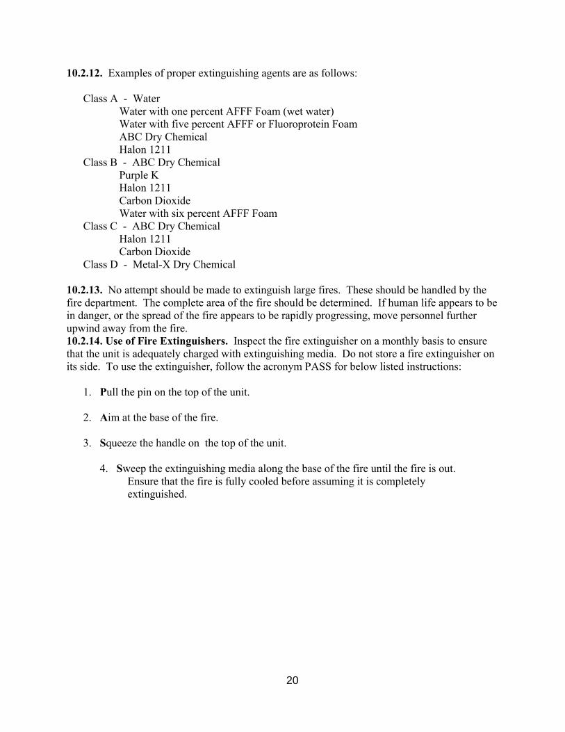
10.2.12. Examples of proper extinguishing agents are as follows: Class A - Water Water with one percent AFFF Foam (wet water) Water with five percent AFFF or Fluoroprotein Foam ABC Dry Chemical Halon 1211 Class B - ABC Dry Chemical Purple K Halon 1211 Carbon Dioxide Water with six percent AFFF Foam Class C - ABC Dry Chemical Halon 1211 Carbon Dioxide Class D - Metal-X Dry Chemical 10.2.13. No attempt should be made to extinguish large fires. These should be handled by the fire department. The complete area of the fire should be determined. If human life appears to be in danger, or the spread of the fire appears to be rapidly progressing, move personnel further upwind away from the fire. 10.2.14. Use of Fire Extinguishers. Inspect the fire extinguisher on a monthly basis to ensure that the unit is adequately charged with extinguishing media. Do not store a fire extinguisher on its side. To use the extinguisher, follow the acronym PASS for below listed instructions: 1. Pull the pin on the top of the unit. 2. Aim at the base of the fire. 3. Squeeze the handle on the top of the unit. 4. Sweep the extinguishing media along the base of the fire until the fire is out. Ensure that the fire is fully cooled before assuming it is completely extinguished.

20

HOSPITALS: FIGURE 4 Barrie: Royal Victoria Hospital 705-728-9802 201 Georgian Dr Barrie, ON L4M 6M2

Directions: Head north out of the base through Angus on Hwy 90 which turns into Dunlop St West once you're in Barrie, exit onto 400 North, take the Georgian St Exit

21

Alliston: Stevenson Memorial Hospital 705-435-6281 200 Fletcher Cres Alliston, ON L9R 1M1

Directions: Take Road 15 out of the Base (heading South), once in Alliston (Road 15 turns into King St) turn left onto Fletcher Cresent, the hospital will be on your left.

22

CFB Borden Road Map

RangeCont r ol

Fi r eHal l

Hospi tal

Canex

McD

Rat ions & Quar ter Suppor t

Bleacher s

To All i ston

Sou th Barrier

North Barrier To Angus

Dieppe Rd

Dieppe Rd

Dieppe R

d

River RdFalaise RdFalaise R

d

Ortona RdOrtona Rd

To UWField Sites

Waterloo R

d

Ram

i lli es Rd

In an emergency go to either Range Control (corner of Falaise and River Roads) or the FireStation (Falaise and Ortona Roads), if it is an emergency the will take you to theBase hospital at the north end of Ortona Rd. If it is not an emergency the will sendyou onto either the Barrie or Alliston Hospitals. The Alliston Hospital is 10 minutes closer thanthe Barrie Hospital, however the Barrie Hospital is considered to be MUCH better.

paramedicsparamedics

23

Documents

Field Demonstration and Validation of a New Device for ... · Field Demonstration and Validation of a New Device for ... SOP Standard operating procedure ... OF THE METER KD IS GREATER