1

The Future of Gas Turbine Technology

7th

International Conference

14-15 October 2014, Brussels, Belgium

Paper ID Number (11)

FIELD MEASUREMENT RECONCILIATION FOR COMBINED CYCLE HEAT

RECOVERY STEAM GENERATOR MONITORING

Alessio Martini Alessandro Sorce Alberto Traverso

alessio.martini@unige.it alessandro.sorce@unige.it alberto.traverso@unige.it

Thermochemical Power Group (TPG), DIME, University of Genoa

Via Montallegro 1, Genoa, Italy

phone:(+39)010353-2463 fax:(+39)010353-2566

ABSTRACT

Long term monitoring and diagnostic of power plants is a

permanent challenge for the energy companies. In particular

with the increase of flexible exercise (e.g. daily start-up and

shut-down cycles, part load operations) the definition of proper

diagnostic indicators becomes mandatory. Different monitoring

strategies were developed, implemented and tested for the main

machineries of combined cycle power plants (e.g. Gas Turbine,

Heat Recovery Steam Generator, Steam Turbine, Pumps) to

prevent fault or failure or to plan/evaluate the maintenance

activities.

This work focuses on the first principles health assessment

of the Heat Recovery Steam Generator (HRSG). At first a brief

analysis about the relationship between the global HRSG

efficiency and the GT net power is presented. From an initial

global study the attention has been addressed to a single

component analysis focusing on the section that involves the

first three heat exchangers in the HRSG gas path (named SH2,

RH and SH1 respectively). This choice has been done for two

main reasons: firstly these heat exchangers are the most

important in terms of quality of energy recovered (higher

temperatures means higher exergies), secondly this section has

the highest number of measurement points which allows

redundancy in energy balances. This second point is the key for

the implementation of an effective validation phase based

on Data Reconciliation and Gross Error Detection in order to

improve the accuracy of the results and show the effectiveness

of such techniques in the power plant monitoring. Several input

set of data have been preprocessed identifying steady-state

conditions and then analyzed and compared to find the

optimal subset of measurements giving the best accuracy of the

results.

INTRODUCTION

Combined Cycle Power Plant (CCPP) performance

analysis is an important topic for the large diffusion of this kind

of systems worldwide. CCPPs, in fact, have the highest

efficiency between the large size power generation systems.

Nowadays the effect of electricity market in Europe leads to a

flexible operation, in which CCPP components are stressed by

high frequency of start up and shut down (even more than one

per day). Additionally fast load ramps are often requested to

support the grid stability. Such operating method has an impact

on the components performance and structural integrity.

The correct evaluation of the efficiency and thus

performance degradation of the whole system and its subsystem

is a valuable method to drive action of condition based

maintenance and in general to optimize the plant operation.

Several analyses can be conducted to monitor the HRSG

functionality:

- performance analysis,

- structural / chemical analysis.

Procedure for the HRSG performance assessment was

presented by Cafaro et al. [1,2] focusing on the evaluation of

diagnostic indicators for real applications; the effect of the GT

degradation on HRSG and cycle performance was discussed by

Zwebek and Pilidis [3].

On the other hand, evaluation of material stresses during

transient are mandatory in the new market scenario. Today’s

analytical techniques to assess transient behavior and the

associated stresses and creep or fatigue damage can be used in a

combination with off-line analysis and on-line monitoring to

better quantify the consequences of this flexible operation,

Bauver and Decoussemaker [4] presented assessment

techniques, inspection methodologies and monitoring tools

focused on HRSG; chemical monitoring of the HRSG and the

main corrosion mechanisms are presented by Dooley [5].

Long term monitoring is a mandatory issue for companies

working in the energy production market, also manufacturers

exploit their deep knowledge of power plant system to create

2

their own monitoring system basing on process data acquired

from all the production units and stored in centralized dedicated

servers.

Supervision strategy for HRSG transient stresses are

already implemented on the DCS Power plants, with the Boiler

Stress Evaluator, moreover operating procedure to reduce

stresses during start-up and shut-down were put in place to face

market requirements minimizing the company assets depletion.

Then the main focus of this work is the performance

monitoring over time. In particular, the effect of Data

Reconciliation on raw data is going to be investigated as an

improvement for results accuracy.

Data Reconciliation exploits the available knowledge about

the process in the form of a model, with the aim of:

- filter data by outlier elimination

- make data consistent

- reduce the measurement uncertainties

The measurements errors are classified typically as:

- Random Error, zero-mean, normally distributed which are

the results of simultaneous effect of several causes. The

combination of this kind of errors during calculation

brings the results to be normally distributed, then subject

to an uncertainty.

- Non-Random Error, usually caused by large, short-term,

non-random events. They can subdivide into:

o measurement-related errors, sensors

malfunctioning

o process-related errors, such as process leak.

Gross Error, are part of the Non-Random Errors and occurs

when measurement device provide consistently erroneous

values, either high or low.

Data Reconciliation deals with random error; its aim is to

align the measurement to their real value, fulfilling the first

principle process equation, such as mass and energy balances as

presented by Romagnoli et al. [6]. The presence of gross errors

invalidates the statistical basis of data reconciliation

procedures. The technique of DR crucially depends on the

assumption that only random errors are present, To verify this

hypothesis, reconciled data are compared to the raw one to

verify with a statistical test that measurement adjustment are

affected by just random error.

NOMENCLATURE

ATT Attemperator

CCPP Combined Cycle Power Plant

DR Data Reconciliation

FHW Feedwater

GED Gross Error Detection

GT Gas Turbine

HP High Pressure

HRSG Heat Recovery Steam Generator

IP Intermediate Pressure

LP Low Pressure

OTC Outlet Temperature Corrected

RH Reheater

SH Superheater

SQP Sequential Quadratic Programming

MONITORING OF THE HRSG PERFORMANCE The heat recover capacity is function of the inlet conditions

(GT exhaust mass flow rate and temperature). The ambient

temperature and the GT load have the major impact on cycle

performance. With the increase of flexible exercise, it is more

common for combined cycle power plants to operate at part

load. Thus, long term monitoring procedures must be able to

consider also significant part-load operating points.

The actual turbine outlet temperature (green triangles)

increases with the reduction of GT load, in order to maintain an

optimized off-design efficiency and low emissions, as shown in

Fig.1. The red and blue lines, which represent the expected

values for the new and clean machine, respectively for exhaust

mass flow rate and temperature, were extracted from the

manufacturer curves. The green triangles and the blue squares

represent the measured or calculated values for steady state and

ISO condition (ambient temperature 15°C, pressure 1.013 bar,

humidity 60%), respectively for exhaust mass flow rate and

temperature.

400

500

600

700

800

100 150 200 250 300

GT

exh

aust

mas

s fl

ow

an

d

tem

ep

ratu

re

GT Load [MW]

GT exhaust mass flow rate actual [kg/s]GT exhaust mass flow rate expected [kg/s]GT exhaust temperature actual [°C]GT exhaust temperature [°C]

Fig.1: Expected and actual exhaust mass flow rate and

temperature vs. GT load

The actual mass flow rate is calculated basing on the GT

first principle balance, taking into account ambient conditions,

fuel mass flow rate, air and gas compositions and discharge

temperature. The outlet temperature is set by the OTC Control,

so the GT degradation affects only the mass flow rate.

A lower GT efficiency results in an increase of heat

released with the exhaust (Fig. 2). A higher heat load to HRSG

is detrimental for its efficiency, which can be overall modeled

as a counter flow heat exchanger as shown by Cafaro [1].

3

250

300

350

400

450

100 150 200 250 300GT

exh

au

st e

ne

rgy

[M

W]

GT Load [MW]

GT exhaust energy actual [MW]

GT exhaust energy expected [MW]

Fig. 2: Expected and actual exhaust energy vs. GT load

To monitor the energetic performance of the overall HRSG

a first principle approach indicator can be defined by eq. (1) as

the ratio of the steam produced by the HRSG and the energy at

the GT outlet

hHRSG =QHRSGs

Q1

e (1)

The GT exhaust energy is obtained through the energy balance

around the GT as shown in eq. (2), taking into account the

combustion chamber efficiency and the GT losses due to

mechanical and electrical efficiency of the bearings and of the

generator respectively. The use of the fuel Low Heating Value

is justified by the discharge temperature, which does not allow

condensation of the flue gas steams.

(1)

The HRSG steam production is evaluated as the sum of the

heats of each pressure level, reheat and feedwater (Fig. 4)

QHRSGs =QHP

s +QIPs +QLP

s +QRHs +QFHW

w (2)

75

77.5

80

82.5

85

87.5

90

100 150 200 250 300

HR

SG e

ffic

ien

cy [

%]

GT Load [MW]

HRSG efficiency actual % HRSG efficiency expected %

Fig. 3: Expected and actual HRSG efficiency for vs. GT load

Fig. 3 shows the HRSG efficiency behavior with respect to

GT load. The expected values (red line) are derived from the

CCPP heat balances solved for different ambient temperatures.

The expected trend can be explained on the basis of the counter

heat exchanger example: with higher ambient temperature the

mass flow rate and thus the total energy entering the HRSG is

reduced. This causes an increase of the specific exchange

surface per unit of mass flow rate. Moreover higher ambient

temperature leads to higher GT exhaust temperature and, since

steam temperatures are controlled through constant values, the

increase of the temperature difference increases the heat

exchanged. The actual HRSG efficiency values (blue squares)

follow the expected trend but are lower because of GT

degradation, which causes the increase in the heat entering the

boiler, with respect to the base line.

Fig. 4: HRSG scheme and mass flow measurements locations

Q1

e =m fuel ×LHV ×hCC +mair ×h0

a -PGT -Plosses

4

DR CONCEPT AND FORMULATION

Globally, DR is a constrained optimization problem

and various resolution methods exist in literature such as

Lagrange Multipliers, successive linear DR, Sequential

Quadratic Programming (SQP) and so on as presented by

Romagnoli et al. [6] and Narasimhan et al. [7]. In this

work a novel resolution technique based on least squares

approach has been applied, having been previously

validated as presented by Coco et al. [8]: it leads to a faster

resolution of the minimization problem (saving about 90%

of computational time compared to the other state of the

art algorithm) and allows the use of the DR tool in larger

set of data or with an higher number of component.

Moreover the methodology can be used for a

combinatorial approach in the Gross Error Identification

phase (serial elimination), where resolution time of the DR

loop is critical.

The general nonlinear Data Reconciliation problem

can be formulated as a least squares minimization problem

as follows:

Minx,u

y- x( )T

S-1 y- x( ) (3)

subject to

f (x,u) = 0 (4)

g(x,u) £ 0 (5)

where

f : m x 1 vector of equality constraints (usually mass and

energy balances);

g : q x 1 vector of inequality constraints (usually variables

bounds);

Σ : n x n variance-covariance matrix;

u : p x 1 vector of unmeasured variables;

x : n x 1 vector of measured variables;

y : n x 1 vector of measured values of measurements of

variables x.

INPUT DATA

The data inputs for the study have been selected at

steady state; averaged value where redundant

instrumentation is employed (e.g. GT outlet temperature,

stack of the HRSG) was selected. The criteria used for

collecting data were: stability of gas turbine and of steam

pressures (controlled parameter). Five minutes time

average was employed to reduce the real scattering of the

field, as reported in the first three figures.

Tab. 1 lists all the variables considered in this study,

specifying the tag, unit, if it is measured of not and the

instrument uncertainty in case of measured variable. The

uncertainties of measured variables are derived from

instrument characteristics; for the gas exhaust temperatures

through the heat exchangers considered in this case study

(T1, T3, T5 and T6), an higher uncertainty has been

considered because they are evaluated through a single

instrument over a great heat exchange area (about 200

squared meters). Besides the radiant heat losses of the heat

exchangers have been considered as measured variables

(their values have been taken as the design values) in order

to improve the redundancy of the DR problem. For this

reason high uncertainties have been assumed, about 10 %.

Variables Unit Measured =

Unmeasured = Uncertainty

Z1 m1 kg/s 1 [%]

Z2 T1 °C 5 [°C]

Z3 m2 kg/s -

Z4 T2 °C -

Z5 m7 t/h -

Z6 T7 °C -

Z7 p7 barg -

Z8 m8 t/h 1 [%]

Z9 T8 °C 2.5 [°C]

Z10 p8 barg 1 [%]

Z11 m3 kg/s -

Z12 T3 K 5 [°C]

Z13 m4 kg/s -

Z14 T4 °C -

Z15 m9 t/h -

Z16 T9 °C 2.5 [°C]

Z17 p9 barg 1 [%]

Z18 m10 t/h -

Z19 T10 °C 2.5 [°C]

Z20 p10 barg 1 [%]

Z21 m5 kg/s -

Z22 T5 °C 5 [°C]

Z23 m6 kg/s -

Z24 T6 °C 5 [°C]

Z25 m11 t/h -

Z26 T11 °C -

Z27 p11 barg 1 [%]

Z28 m12 t/h -

Z29 T12 °C -

Z30 p12 barg -

Z31 m13 t/h 1 [%]

Z32 T13 °C 2.5 [°C]

Z33 p13 barg 1 [%]

Z34 m14 t/h -

Z35 T14 °C -

Z36 p14 barg -

Z37 m15 t/h -

Z38 T15 °C -

Z39 p15 barg -

Z40 QradSH2 kW 10 [%]

Z41 QradRH kW 10 [%]

Z42 QradSH1 kW 10 [%]

Tab. 1: Variables considered in the DR problem

5

DR PROBLEM APPLIED TO A SPECIFIC HRSG

SECTION

After a global analysis on HRSG efficiency behavior

vs. GT load, we focused on the first three heat exchangers

(SH2, RH, SH1) of the HRSG. These heat exchangers are

the most important in terms of quality of energy recovered

(higher temperatures means higher exergies). For this

reason, this section has several measurement points which

allows redundancy in energy balances. So DR has been

applied to the first three heat exchangers (SH2, RH, SH1)

of the HRSG. The simplified layout is shown in Fig. 5.

In this DR problem there are 42 variables, 19

measured and 23 unmeasured, as shown in Tab. 1.

Fig. 5: Layout of the first three HRSG heat exchangers

A steady state DR based on mass and energy balances

was developed. Moreover, the pressure drop equation has

been considered for each heat exchanger. The saturation

temperature equation in function of saturation pressure has

also been considered for the steam at the first superheater

(SH1_HP) inlet. Finally, all the equations related to the

connection nodes have been considered (in this case study

there are 4 nodes).

The total number of process equations is 26; they are

listed for each component in the followings.

SH2_HP (High Pressure Superheater 2)

m1 -m2 = 0 (6)

m7 -m8 = 0 (7)

m1 ×h1 -m2 ×h2 +m7 ×h7 -m8 ×h8 -QradSH 2HP = 0 (8)

p7 - p8 -Dp m7,T7,T8( ) = 0

(9)

RH_IP (Intermediate Pressure Reheater)

m3 -m4 = 0 (10)

m9 -m10 = 0 (11)

m3 ×h3 -m4 ×h4 +m9 ×h9 -m10 ×h10 -QradRHIP = 0 (12)

p9 - p10 -Dp m9,T9,T10( ) = 0

(13)

SH1_HP (High Pressure Superheater 1)

m5 -m6 = 0 (14)

m11 -m12 = 0 (15)

m5 ×h5 -m6 ×h6 +m11 ×h11 -m12 ×h12 -QradSH1HP = 0 (16)

p11 - p12 -Dp m11,T11,T12( ) = 0

(17)

T11 -Tsat (p11) = 0

(18)

ATT_SH (Superheater attemperator)

m14 +m13 -m15 = 0 (19)

m14 ×h14 +m13 ×h13 -m15 ×h15 = 0 (20)

p14 - p15 = 0

(21)

Node 2-3

m2 -m3 = 0 (22)

T2 -T3 = 0 (23)

Node 4-5

m4 -m5 = 0 (24)

T4 -T5 = 0 (25)

Node 15-7

m15 -m7 = 0 (26)

T15 -T7 = 0 (27)

p15 - p7 = 0

(28)

Node 12-14

m12 -m14 = 0 (29)

T12 -T14 = 0 (30)

p12 - p14 = 0

(31)

As aforementioned in the previous section, the radiant heat

losses of the heat exchangers have been considered as measured variables. This allows the degrees of freedom in

the DR problem to be greater than zero, in particular equal

to 3 being the difference between the number of equations

26 and the number of observable unmeasured variables 23.

6

STATISTICAL GED

The statistical component of a GED strategy simply

attempts to answer the question of whether gross errors are

present in the data or not. It does not provide any insight

on either the number of gross errors, their types, or their

locations. All detection methods, either directly or

indirectly, utilize the fact that gross errors in measurements

cause them to violate the model constraints. If

measurements do not contain any random errors, then a

violation of any of the model constraints by the measured

values can be immediately interpreted as due to the

presence of gross errors. This is a purely deterministic

method.

The most commonly used statistical techniques for

detecting gross errors are based on hypothesis testing. In a

GED case, the null hypothesis H0 is that no gross error is

present, and the alternative hypothesis H1 is that one or

more gross errors are present in the system. All statistical

techniques for choosing between these two hypotheses

make use of a test statistic, which is a function of the

measurements and constraint model. The test statistic is

compared with a pre-specified threshold value and the null

hypothesis is rejected or accepted, respectively, depending

on whether the statistic exceeds the threshold or not. The

threshold value is also known as the test criterion or the

critical value of the test. The outcome of hypothesis testing

is not perfect. A statistical test may declare the presence of

gross errors, when in fact there is no gross error (H0 is

true). In this case, the test commits a Type I error or gives

rise to a false alarm. On the other hand, the test may

declare the measurements to be free of error, when in fact

one or more gross errors exists (Type II error). The power

of a statistical test, which is the probability of correct

detection, is equal to 1-Type II error probability. The

power and Type I error probability of any statistical test

are intimately related. By allowing a larger Type I error

probability, the power of a statistical test can be increased.

Therefore, in designing a statistical test, the power of the

test must be balanced against the probability of false

detection. If the probability distribution of the test statistic

can be obtained under the assumption of the null

hypothesis, then the test criterion can be selected so that

the probability of Type I error is less than or equal to a

specified value . The parameter is also referred to as

the level of significance for the statistical test.

The global test, which was the first test proposed

[9,10,11], uses the test statistic given by the following

equation

g = rT ×V -1 × r (11)

where r is the vector of balance residuals given by

r = Jx × y- x( ) (12)

where Jx is the jacobian matrix with respect measured

variables, y is the vector of measurements and x is the

vector of reconciled values.

In the absence of gross errors, the vector r follows a

multivariate normal distribution with zero mean value and

variance-covariance matrix V given by

V = cov(V ) = Jx × S× JxT

(13)

In the presence of gross errors, the elements of

residual vector r reflect the degree of violation of process

constraints (material and energy conservation laws). On

the other hand, matrix V contains information of the

process structure (matrix Jx) and the measurement

variance-covariance matrix, Σ. The two quantities, r and V,

can be used to construct statistical tests which can detect

the existence of gross errors. Under the null hypothesis H0,

the above statistic follows a 2

(chi-square) distribution

with degrees of freedom. If the test criterion is chosen as 2

,1 , where

2

,1 is the critical value of

2

distribution at the chosen level of significance, then H0

is rejected and a gross error is detected, if

g ³ c1-a,n

2 (14)

This choice of the test criterion ensures that the

probability of Type I error for this test is less than or equal

to . The global test combines all the constraint residuals

in obtaining the test statistic, and therefore gives rise to a

multivariate or collective test that embodies the process

knowledge.

This statistical approach is used to filter out data that

are not consistent with the equations (for this work a

degree of 95% of significance was chosen).

RESULTS

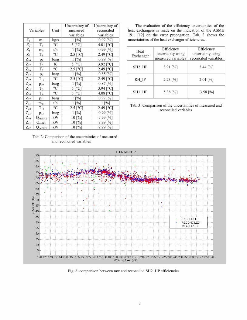
Fig. 6, 7 and 8 show a comparison between the raw

(red) and reconciled values (blue) of the heat exchangers

efficiencies SH2_HP, RH_IP and SH1_HP, respectively.

The green values are related to the efficiencies discarded

after the reconciliation process, because of the high value

of the test statistic γ. This indicator gives a suggestion of

the correction that have to be added to the measured data

set to fulfill the energy balance equation. When γ exceeds

the statistical threshold chi-square, a gross error is detected

and the measured data set is discarded as not reconcilable.

It can be noticed that the data DR reduces the efficiency

scattering as well as the final uncertainties.

Tab. 2 presents a comparison of the uncertainties of

measured and reconciled variables.

7

Variables Unit

Uncertainty of

measured

variables

Uncertainty of

reconciled

variables

Z1 m1 kg/s 1 [%] 0.97 [%]

Z2 T1 °C 5 [°C] 4.01 [°C]

Z8 m8 t/h 1 [%] 0.99 [%]

Z9 T8 °C 2.5 [°C] 2.49 [°C]

Z10 p8 barg 1 [%] 0.99 [%]

Z12 T3 K 5 [°C] 3.92 [°C]

Z16 T9 °C 2.5 [°C] 2.49 [°C]

Z17 p9 barg 1 [%] 0.85 [%]

Z19 T10 °C 2.5 [°C] 2.49 [°C]

Z20 p10 barg 1 [%] 0.87 [%]

Z22 T5 °C 5 [°C] 3.94 [°C]

Z24 T6 °C 5 [°C] 4.08 [°C]

Z27 p11 barg 1 [%] 0.97 [%]

Z31 m13 t/h 1 [%] 1 [%]

Z32 T13 °C 2.5 [°C] 2.49 [°C]

Z33 p13 barg 1 [%] 0.99 [%]

Z40 QradSH2 kW 10 [%] 9.99 [%]

Z41 QradRH kW 10 [%] 9.99 [%]

Z42 QradSH1 kW 10 [%] 9.99 [%]

Tab. 2: Comparison of the uncertainties of measured

and reconciled variables

The evaluation of the efficiency uncertainties of the

heat exchangers is made on the indication of the ASME

19.1 [12] on the error propagation. Tab. 3 shows the

uncertainties of the heat exchanger efficiencies.

Heat

Exchanger

Efficiency

uncertainty using

measured variables

Efficiency

uncertainty using

reconciled variables

SH2_HP 3.91 [%] 3.44 [%]

RH_IP 2.23 [%] 2.01 [%]

SH1_HP 5.38 [%] 3.58 [%]

Tab. 3: Comparison of the uncertainties of measured and

reconciled variables

Fig. 6: comparison between raw and reconciled SH2_HP efficiencies

8

Fig. 7: comparison between raw and reconciled RH_IP efficiencies

Fig. 8: comparison between raw and reconciled SH1_HP efficiencies

9

CONCLUSIONS

In this work the effect of data reconciliation on long

term monitoring data was presented and tested. First of

all, the relation between GT load and HRSG efficiency

was highlighted. A Data Reconciliation problem was set

implementing energy balance equation around each one

of the first three heat exchangers of HRSG.

It was proven that DR is an effective instrument to:

filter data by outlier elimination

make data consistent

reduce the measurement uncertainties

The effects of these enhancements were shown on the

target indicators: the heat exchanger efficiencies

SH2_HP, RH_IP and SH1_HP respectively.

These efficiencies are characterized by the same

decreasing trend of the global HRSG efficiency indicator

with respect to GT load.

ACKNOWLEDGMENTS

This work has been carried out in the framework of

research activities on energy systems diagnostics, which

are partially founded by Ansaldo Energia SpA, which is

greatly acknowledged.

REFERENCES

[1] Cafaro S., Traverso A., Massardo A., 2009, Heat

recovery steam generator performance and

degradation in a 400MWcombined cycle, Proc.

IMechE Vol. 223 Part A: J. Power and Energy, pag.

369-378.

[2] Cafaro S., Veer T., 2009 "Diagnostics of Combined

Cycle Power Plants: Real Applications to Condition

Based Maintenance", 9th International Conference

on Heat Engines and Environmental Protection.

[3] Zwebek A. I., Pilidis P., 2001, “Degradation Effects

on Combined cycle Power Plant Performance, Part

2: Steam Turbine Cycle Component Degradation

Effects”. ASME Paper 2001-GT-389.

[4] Decoussemaeker P., Bauver W., “Asset management

and condition monitoring for HRSG that are

confronted with increasing cycling”, IGTC2012-6,

6th International Conference 17-18 October 2012,

Brussels, Belgium.

[5] Dooley B., Anderson B., “HRSG assessments

identify trends in cycle chemistry, thermal transient

performance”, Combined Cycle Journal, I-2009,

115-130.

[6] Romagnoli, J.A., Sanchez, M.C., "Data Processing

and Reconciliation for Chemical Process

Operations", Academic Press, London (2000).

[7] Narasimhan S., Jordache C., “Data Reconciliation

and Gross Error Detection: an intelligent use of

process data”. Gulf Publishing Company, Houston,

Texas, 2000.

[8] Coco D., Martini A., Sorce A., Traverso A.,

Levorato P., 2013 "Data reconciliation: an

engineeristic approach based on least squares

optimization", 5th International Conference of

Applied Energy (ICAE), Pretoria, South Africa.

[9] Ripps, D. L. "Adjustment of Experimental Data."

Chem. Eng. Progress Symp. Series 61 (1965): 8-13.

[10] Almasy G. A., Sztano T., (1975), "Checking and

Correction of Measurements on the Basis of Linear

System Model." Problems of Control and

Information Theory 4: 57-69.

[11] Madron, F. "A New Approach to the Identification

of Gross Errors in Chemical Engineering

Measurements." Chem. Eng. Sci. 40 (1985): 1855-

1860.

[12] ASME 19.1, 1985, Measurement Uncertainty

(Instruments and Apparatus).