Embed Size (px)
Citation preview
OCS Study BOEM 2018-029
Field Observations During Wind Turbine Foundation Installation at the Block Island Wind Farm, Rhode Island
Appendix F: Turbine Scour Monitoring Report
US Department of the Interior Bureau of Ocean Energy Management Office of Renewable Energy Programs

OCS Study BOEM 2018-029
Field Observations During Wind Turbine Foundation Installation at the Block Island Wind Farm, Rhode Island Appendix F: Turbine Scour Monitoring Report
May 2018 Authors (in alphabetical order): Jennifer L. Amaral, Robin Beard, R.J. Barham, A.G. Collett, James Elliot, Adam S. Frankel, Dennis Gallien, Carl Hager, Anwar A. Khan, Ying-Tsong Lin, Timothy Mason, James H. Miller, Arthur E. Newhall, Gopu R. Potty, Kevin Smith, and Kathleen J. Vigness-Raposa Prepared under BOEM Award Contract No. M15PC00002, Task Order No. M16PD00031 By HDR 9781 S Meridian Boulevard, Suite 400 Englewood, CO 80112
U.S. Department of the Interior Bureau of Ocean Energy Management Office of Renewable Energy Programs

OCS Study
BOEM 2018
Scour Monitoring at the Block Island Wind Farm, Rhode Island
US Department of the Interior Bureau of Ocean Energy Management Office of Renewable Energy Programs

OCS Study BOEM 2018
Scour Monitoring at the Block Island Wind Farm, Rhode Island
March 2018
Authors:
Fugro GB Marine Limited
Coastal Oceanography Department
Trafalgar Wharf (Unit 16)
Hamilton Road
Portchester PO6 4PX
United Kingdom
Prepared under BOEM Award
Contract No. M15PC00002
Task Order No. M15PD00029 By HDR 9781 S Meridian Blvd, Suite 400 Englewood, CO 80112
US Department of the Interior Bureau of Ocean Energy Management Office of Renewable Energy Programs

DISCLAIMER
This report was prepared under contract between the Bureau of Ocean Energy Management (BOEM)
and HDR EOC. This report has been technically reviewed by BOEM and has been approved for
publication. Approval does not signify that the contents necessarily reflect the views and policies of
BOEM, nor does mention of trade names or commercial products constitute endorsement or
recommendations for use. It is, however, exempt from review and in compliance with BOEM editorial
standards.
REPORT AVAILABILITY
The report may be downloaded from the boem.gov website through the Environmental Studies
Program Information System (ESPIS). You will be able to obtain this report from BOEM or the
National Technical Information Service by writing to the following addresses.
U.S. Department of the Interior U.S. Department of Commerce
Bureau of Ocean Energy Management National Technical Information Service
Office of Renewable Energy Programs 5285 Port Royal Road
45600 Woodland Road Springfield, Virginia 22161
Sterling, Virginia 20166 Phone: (703) 605-6040
Fax: (703) 605-6900
Email: [email protected]
CITATION
HDR. 2018. Scour Monitoring at the Block Island Wind Farm, Rhode Island. Final Report to the U.S.
Department of the Interior, Bureau of Ocean Energy Management, Office of Renewable Energy
Programs. OCS Study BOEM 2018.
ABOUT THE COVER
Cover photo: BIWF scour monitors. Photo by HDR RODEO Team.

i
Contents
List of Figures ............................................................................................................................................. ii
List of Tables .............................................................................................................................................. iii
List of Abbreviations and Acronyms ....................................................................................................... iv
1 Introduction ......................................................................................................................................... 5
1.1 Deployment Position and Dates ................................................................................................... 5
1.2 Project Aims and Results .............................................................................................................. 7
2 AWAC Configuration Information ..................................................................................................... 8
3 Scour Configuration Information ...................................................................................................... 9
4 Data Collection .................................................................................................................................. 10
4.1 Data Return ................................................................................................................................. 10
4.2 Oceanographic Data Summary .................................................................................................. 10
4.2.1 Water Levels ........................................................................................................................ 10
4.2.2 Currents ................................................................................................................................ 10
4.2.3 Waves................................................................................................................................... 12
4.3 Seabed Data Summary .............................................................................................................. 14
4.3.1 Long Term Trends ................................................................................................................ 14
4.3.2 Short Term Trends ............................................................................................................... 20

ii
List of Figures
Figure 1. Location of Deployed Equipment ................................................................................................ 5
Figure 2. Winter Water Level Data - Height to Lowest Astronomic Tide and Residuals .......................... 11
Figure 3. January 2017 Current Data – Observed and Non-tidal Components ....................................... 11
Figure 4. All current data – progressive vector plot .................................................................................. 12
Figure 5. All Wave Data – Significant Wave Height Versus Coming Direction Hodogram (rose
plot) ........................................................................................................................................... 13
Figure 6. March 2017 Wave Data ............................................................................................................ 13
Figure 7. SE Beam 1 Scour Depth ........................................................................................................... 15
Figure 8. Figure 4.7: SE Beam 2 Scour Depth ......................................................................................... 15
Figure 9. SE Beam 3 Scour Depth ........................................................................................................... 16
Figure 10. SE Beam 4 Scour Depth ........................................................................................................... 16
Figure 11. NE Beam 1 Scour Depth ........................................................................................................... 17
Figure 12. NE Beam 2 Scour Depth ........................................................................................................... 17
Figure 13. NE Beam 3 Scour Depth ........................................................................................................... 18
Figure 14. NE Beam 4 Scour Depth ........................................................................................................... 18
Figure 15. Significant Wave Height ............................................................................................................ 19
Figure 16. Depth Average Velocity ............................................................................................................. 19
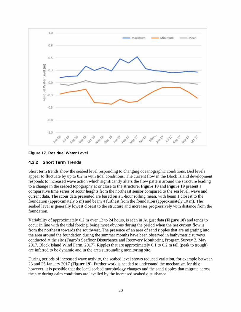
Figure 17. Residual Water Level ................................................................................................................ 20
Figure 18. Comparative time series for August 2016 ................................................................................. 21
Figure 19. Comparative time series for January 2017 ............................................................................... 21

iii
List of Tables
Table 1. Equipment Positions – Deployment ............................................................................................ 6
Table 2. Equipment Positions – Service 1 ................................................................................................ 6
Table 3. Equipment Positions – Service 2 ................................................................................................ 6
Table 4. Equipment Positions – Service 3 ................................................................................................ 6
Table 5. Equipment Positions – Recovery ................................................................................................ 6
Table 6. AWAC Summary Information ...................................................................................................... 8
Table 7. Scour Monitor Summary ............................................................................................................. 9
Table 8. Data Return Summary .............................................................................................................. 10
Table 9. Monthly Significant Wave Height Statistics ............................................................................... 14

iv
List of Abbreviations and Acronyms
AWAC Acoustic Wave and Current Profiler
CTD Salinity, Temperature and Depth
MLW Mean Low Water
UTC Coordinated Universal Time
WGS84 World Geodetic System, 1984
WTG Wind Turbine Generator

5
1 Introduction
As part of the assessment of the Block Island Wind Farm Installation, Fugro was contracted by HDR
Environmental, Operations and Construction Inc. (HDR) to study scour around a turbine. The survey
involved the installation of two scour monitors on opposite legs of Platform 3 (WTG3) (Figure 1 and
Tables 1 to 5). The scour monitors measure changes in seabed elevation around the base of the jacket
legs.
An acoustic wave and current (AWAC) profiler was also deployed in a seabed frame approximately 500
m southeast of the turbine (Figure 1 and Tables 1 to 5). The wave, water level and current data collected
by the AWAC have been used to inform an assessment of the factors affecting seabed level changes as
measured by the scour monitors.
AWAC and scour monitor configurations are presented in Tables 6 and 7, respectively. Both units were
originally intended to be installed for a period of at least nine months, with maintenance scheduled at
approximately three-month intervals. The contract was then extended for a further three months.
1.1 Deployment Position and Dates
Figure 1. Location of Deployed Equipment

6
Table 1. Equipment Positions – Deployment
Location Name
Latitude (WGS84)
Longitude (WGS84)
UTM Coordinates (NAD83 Zone 19 N)
Deployment Date
Seabed Frame 41° 06’ 34.5” N 071° 31’ 00.5” W 288674.5 m E, 4553973.8 m N 15 June 2016
Anchor Weight 41° 06 ’36.2” N 071° 31’ 01.1” W 288662.0 m E, 4554026.6 m N 15 June 2016
Scour Monitors (WTG3)
41° 06’ 54.0” N 071° 31’ 15.6” W 288339.6 m E, 4554585.4 m N 28 July 2016
Table 2. Equipment Positions – Service 1
Location Name Latitude (WGS84)
Longitude (WGS84)
UTM Coordinates (NAD83 Zone 19 N)
Deployment Date
Seabed Frame 41° 06’ 34.1” N 071° 30’ 59.2” W 288703.2 m E, 4553962.3 m N 10 November 2016
Anchor Weight 41° 06’ 35.9” N 071° 31’ 00.7” W 288670.4 m E, 4554016.9 m N 10 November 2016
Scour Monitors (WTG3)
41° 06’ 54.0” N 071° 31’ 15.6” W 288339.6 m E, 4554585.4 m N 08 November 2016
Table 3. Equipment Positions – Service 2
Location Name Latitude (WGS84)
Longitude (WGS84)
UTM Coordinates (NAD83 Zone 19 N)
Deployment Date
Seabed Frame 41° 06’ 35.9” N 071° 31’ 00.7” W 288671.0 m E, 4554018.1 m N 06 March 2017
Anchor Weight 41° 06’ 34.1” N 071° 31’ 00.7” W 288669.4 m E, 4553962.6 m N 06 March 2017
Scour Monitors (WTG3)
41° 06’ 54.0” N 071° 31’ 15.6” W 288339.6 m E, 4554585.4 m N 21 March 2017
Table 4. Equipment Positions – Service 3
Location Name
Latitude (WGS84)
Longitude (WGS84)
UTM Coordinates (NAD83 Zone 19 N)
Deployment Date
Seabed Frame 41° 06’ 34.1” N 071° 30’ 59.3” W 288703.2 m E, 4553962.3 m N 15 June 2017
Anchor Weight 41° 06’ 36.2” N 071° 31’ 00.8” W 288668.1 m E, 4554028.6 m N 15 June 2017
Scour Monitors (WTG3)
41° 06’ 54.0” N 071° 31’ 15.6” W 288339.6 m E, 4554585.4 m N 14 June 2017
Table 5. Equipment Positions – Recovery
Location Name Latitude (WGS84)
Longitude (WGS84)
UTM Coordinates (NAD83 Zone 19 N)
Recovery Date
Seabed Frame 41° 06’ 34.6” N 071° 30’ 59.6” W 288695.5 m E, 4553976.3 m N 21 October 2017
Anchor Weight 41° 06’ 36.6” N 071° 31’ 01.0” W 288664.7 m E, 4554038.9 m N 21 October 2017
Scour Monitors (WTG3)
41° 06’ 54.0” N 071° 31’ 15.6” W 288339.6 m E, 4554585.4 m N 17 October 2017

7
1.2 Project Aims and Results
The key aims of the project can be summarized as follows:
To generate a 12-month data set of seabed elevation and oceanographic data;
To test the concept of monitoring scour with fixed acoustic instrumentation;
To inform on the possible use of the systems in future developments.
The general outcomes of the study were as follows:
The scour monitoring equipment was installed on WTG3 for a period in excess of 14 months and
provided a near continuous data set for the duration of the deployment;
A seabed mounted wave, current, temperature and water level monitoring station returned a data
set of over 16 months covering the entire period of observations by the scour monitors;
The scour monitors returned the following data:
Continuous acoustic return data along four beams per instrument;
Seabed elevations at distance up to 10 m from foundation;
Changes in the seabed elevation were seen to occur at a variety of periodicities:
Less than one day, consistent with the periodicity of the local tidal forcing;
Over the course of a week to a month, appearing to coincide with perturbations to
the tidal current flow resulting from increased wave energy;
A seasonal signal consistent with increased wave activity in the winter months,
and calmer conditions in the summer months.
The orientation of the acoustic beams allowed observation of the variation in seabed level
with distance from the foundation, and response of the seabed to physical ocean
oceanographic forcing.
Issues encountered with the scour data:
Orientation of the scour monitor on the southeast leg meant the data were collected closer
to the foundation than planned;
Corruption of one scour monitor beam on the southeast leg occurred during the final three
months, probably due interference from the structure.
Lessons learnt:
Early interaction with construction team is vital to allow bracketing to be mounted and
orientated correctly;
At sites with a strong seasonal thermocline it is essential for long term variation in the
seabed levels to be calculated using a speed of sound derived from a model of (or average
of) the conditions between the scour monitor and the seabed. In this case the presence of
a strong summer thermocline caused errors in the initial range calculations. Vertical CTD
profiles taken in the summer months showed that the thermocline depth was
approximately midway between the scour monitor and the seabed. Thus, the average
speed of sound between the scour monitor and the seabed AWAC was calculated and
used to correct the acoustic ranges.
Future opportunities:
The scour monitors provide a long-term time series of seabed elevations at specific points
close to the foundation (in this case up to 10 m) that can be used to enhance the
understanding of the variation in seabed levels;
The scour monitors allow measurement of the seabed response in conditions where
bathymetric surveys are not feasible;
For future sites the scour monitors could be used at a limited selection of foundations in
order to support the assumptions about seabed mobility made during design, or if scour
occurs under specific circumstances then appropriate preventative intervention can be
designed and actioned to maximize the life of the structures.

8
2 AWAC Configuration Information
Table 6. AWAC Summary Information
Block Island AWAC
Serial numbers AWAC: WAV 6058 / WPR 1457 WAV 6133 / WPR 1444 LRT: 216060-002 SMB: EMU 1188 Lantern: EMU 1361 Buoy tracker: 744906 958629
AWAC configuration
Instrument frequency: 600 kHz
Current profile interval: 600 s Cells: 38 Cell size: 1 m Waves samples: 1024 at 1 Hz Wave sample interval: 3600 s Currents averaging period: 60 s Blanking distance: 1 m Coordinate system: Beam Power level: High Assumed duration: 90 days Estimated depth: 38 m Battery: Estimated utilization 78 %
Memory required: 58.1 MB of > 300 MB
Mooring The seabed frame was attached to a 75 m 12.7 mm greased galvanized steel ground line using two 4 tonne rated stainless steel shackles and a 2 tonne rated stainless steel shackle. The ground line was attached to a 500 kg scrap chain anchor using 3.25 tonne Crosby safety shackles. The anchor was connected to a 50 m 12.7 mm greased galvanized steel riser wire using a 3.25 tonne Crosby safety shackle. The riser was attached to a 2 m 16 mm galvanized steel chain with a 3.25 tonne Crosby safety shackle to the surface marker buoy.
Surface marker buoy
Mobilis 1200 yellow buoy 1.2 m diameter and 1.5 m in height. Top mounted solar charging navigational light was configured with the following flash pattern: 5 (y) in 20 (s)
Seabed frame and AWAC Surface marker buoy

9
3 Scour Configuration Information
Table 7. Scour Monitor Summary
Block Island Scour Monitors
Location WTG3
Serial numbers North East: AQD 12905; North East: AQD 13444
South East: AQD 12892; South East: AQD 13429
Scour monitor configuration Instrument frequency: 1 MHz
Cells: 96
Cell size: 0.35 M
Blanking distance: 0.36 M
Coordinate system: Beam
Power level: Low
Assumed duration: 90 days
Depth of site (to MLW): 26.23 m
Depth of instrument (to (MLW): 8.73 m
Installation details Each instrument was secured into its housing by means of stainless steel jubilee clips. The housing comprises of a stainless-steel tube for protecting the instrument and an external locating plate designed to fit onto a mounting bracket. The mounting brackets are permanently installed on the turbine. During the installation the locating plate was attached to the mounting bracket and secured by divers. An anode was also attached to each housing prior to installation.
Scour monitor in bracketing

10
4 Data Collection
4.1 Data Return
Due to weather and other delays, an increased total quantity of data was collected by both the scour
monitors and AWAC, as shown in Table 8. Data have been examined and only those records that pass all
quality control tests are included in the data summary below.
Table 8. Data Return Summary
Deployment Data Collected – AWAC Data Collected – Scour Monitors
1 4 months and 24 days 3 months and 3 days
2 3 months and 26 days 4 months and 10 days
3 3 months and 9 days 3 months and 3 days
4 4 months and 6 days 4 months and 3 days
Overall 16 months and 3 days 14 months and 19 days
4.2 Oceanographic Data Summary
4.2.1 Water Levels
The Block Island tidal environment is dominated by the open ocean tidal signal, and is therefore
characterized by a semidiurnal microtidal (less than 2 m range) signal. The mean spring range is 1.07 m
and the mean high water to mean low water interval difference is 6.13 hours, thus the tide curve is near
symmetrical. The autumn and winter months show multiple periods of non-tidal (residual) sea level
variations. Figure 2 presents an extract of the sea level observations and the calculated non-tidal values
from a 60-point harmonic analysis of the 16 months of data. The residual values vary by up to ±0.5 m and
are thus approximately the same range as the astronomically forced tide. The form of these appear to
indicate two potential forcing processes:
Short to medium term suppression or enhancement of the sea level resulting from atmospheric
forcing, either variations in atmospheric pressure or wind enhancement;
24- to 48-hour oscillations in the residuals that are indicative of a coastally-trapped (or Kelvin)
wave, however additional data and analysis would be needed to correctly define these.
4.2.2 Currents
The current data recorded at the study location were orientated along a northeast – southwest axis. The
maximum expected depth average tidal current is predicted to be less than 0.4 m/s, based on the results of
a 60-point harmonics analysis. The non-tidal component of the flow exceeds the tidal component. Figure
3 presents the depth average observed current and the non-tidal component, which is of the same
magnitude as the observations on multiple occasions. This indicates that atmospheric forcing of the
current is dominant in the study area.
In order to understand the general flow pattern in the study area the data are presented as a progressive
vector plot in Figure 4. The data are shown as total water movement past the measurement point, with a
label added at 28-day intervals. The summer months show a progressive movement of the water mass to
the southwest, which changes to a general motion to the east during the winter months.

11
Figure 2. Winter Water Level Data - Height to Lowest Astronomic Tide and Residuals
Figure 3. January 2017 Current Data – Observed and Non-tidal Components

12
Figure 4. All current data – progressive vector plot
4.2.3 Waves
The Block Island Offshore Wind Farm is sheltered by Block Island and the mainland to the north and
west, thus the wave climate is dominated by waves coming from the south and east. Figure 5 presents a
hodogram (rose plot) of the significant wave height against the direction for all observations. Figure 6
presents an example time series of the wave heights, periods and coming directions for March 2017. The
wave climate during the measurement campaign was seasonal with wave heights not exceeding 3 m for
the months of June, July and August, increasing through autumn to spring; the largest wave recorded was
observed in March.

13
Figure 5. All Wave Data – Significant Wave Height Versus Coming Direction Hodogram (rose plot)
Figure 6. March 2017 Wave Data
HDR Environmental, Operations and Construction, Inc. Wav e Data Hodogram (Rose Diagram)Block Island Wind Farm: Fugro Scour Monitors, WTG 3, Deployment 1-4
Current Meter / AWAC Storm DataLatitude: 41°06'N Longitude: 071°31'W Approximate Site depth below LAT: 26.8m Instrument height off seabed: 0.6m
Serial No.: 1444/1457/1444/1457Deployed: 15/06/2016 15:09 Recovered: 21/10/2017 13:35
Fugro GB Marine Limited Coastal Oceanography Job No: 160215
Coming Direction (°T)
True North
South
West East
Significant Wave Height (m)
0.5 1.0 1.5 2.0 2.5 3.0 3.5 4.0 4.5 5.0 5.5 6.0 6.5 7.0 (m)
Percentage Occurrence
0 5% 10% 15% 20%

14
Table 9 presents a summary of the significant wave heights for each month and the number of storm
events observed (a storm event was defined as any period were significant wave height exceeded 3 m for
this report). The seasonality of the reported events is clear with the highest number recorded in January
and through the winter months; however, there is a second smaller peak in September, coincident with the
period of anticipated hurricane activity. The duration of storm events observed in September appear to be
of longer duration than those in the winter months. However, the duration of the data is insufficient to
confirm the statistical significance of this observation.
Table 9. Monthly Significant Wave Height Statistics
Month Maximum
(m) Mean (m)
Minimum (m)
Average number of events with significant wave height > 3m, and approximate total duration
January 4.74 1.507 0.38 4 events 40 hours
February 5.24 1.228 0.32 2 events 24 hours
March 6.04 1.407 0.32 3 events 60 hours
April 3.63 1.307 0.32 2 events 23 hours
May 3.06 1.189 0.36 1 event 1 hour
June 2.3 0.999 0.36 0 events (in 2 months)
July 2.14 0.886 0.38 0 events (in 2 months)
August 2.89 0.913 0.37 0 events (in 2 months)
September 3.5 1.396 0.4 2 events 40 hours (in 2 months)
October 3.28 1.254 0.31 1 event 3 hours (in 2 months)
November 2.94 1.209 0.39 0 events
December 3.44 1.385 0.32 2 events 24 hours
4.3 Seabed Data Summary
4.3.1 Long Term Trends
Figure 7 to Figure 10 and Figure 11 to Figure 14 present a temporal summary of seabed level data from
beam 1 to 4 for SE and NE scour monitors, respectively. Beam 1 is orientated at an angle of 5° and
therefore represents measurements taken closest to the turbine. In contrast beam 4 is orientated at an angle
of 20° and represents measurements taken furthest from the turbine. Scour data from the SE leg contained
higher levels of interference, which resulted in a loss of the seabed return signal for the 5° beam during
the fourth deployment. Thus, summary statistics from the SE leg are unreliable during July, September
and October 2017. The NE leg showed relatively little interference and data were thus available for all
month on all beams.
Figure 15 to Figure 17 present a temporal summary of oceanographic data from the AWAC.
Measurements from both SE and NE units show a slow reduction in the monthly mean seabed level by
around 0.2 m over 14 months. The range of seabed levels (monthly maximum and minimum) exhibit a
variation of up to 0.6 m over the month. There appears some correlation between the greatest levels of
scour and the highest significant wave heights as measured by the AWAC. It is possible that increased
wave action during the winter and early spring lead to reductions in seabed level. Some recovery of the
seabed level is seen, particularly on the SE leg. This may be due to increased deposition of sediments
following winter conditions close to the foundation. The NE unit shows a small recovery of the mean
seabed level (<0.1 m) during the summer months, July to September, but does not recover to the levels
observed at the start of the study.

15
Figure 7. SE Beam 1 Scour Depth
Figure 8. Figure 4.1: SE Beam 2 Scour Depth

16
Figure 9. SE Beam 3 Scour Depth
Figure 10. SE Beam 4 Scour Depth

17
Figure 11. NE Beam 1 Scour Depth
Figure 12. NE Beam 2 Scour Depth

18
Figure 13. NE Beam 3 Scour Depth
Figure 14. NE Beam 4 Scour Depth

19
Figure 15. Significant Wave Height
Figure 16. Depth Average Velocity
20
Figure 17. Residual Water Level
4.3.2 Short Term Trends
Short term trends show the seabed level responding to changing oceanographic conditions. Bed levels
appear to fluctuate by up to 0.2 m with tidal conditions. The current flow in the Block Island development
responds to increased wave action which significantly alters the flow pattern around the structure leading
to a change in the seabed topography at or close to the structure. Figure 18 and Figure 19 present a
comparative time series of scour heights from the northeast sensor compared to the sea level, wave and
current data. The scour data presented are based on a 3-hour rolling mean, with beam 1 closest to the
foundation (approximately 5 m) and beam 4 furthest from the foundation (approximately 10 m). The
seabed level is generally lowest closest to the structure and increases progressively with distance from the
foundation.
Variability of approximately 0.2 m over 12 to 24 hours, is seen in August data (Figure 18) and tends to
occur in line with the tidal forcing, being most obvious during the period when the net current flow is
from the northeast towards the southwest. The presence of an area of sand ripples that are migrating into
the area around the foundation during the summer months have been observed in bathymetric surveys
conducted at the site (Fugro’s Seafloor Disturbance and Recovery Monitoring Program Survey 3, May
2017, Block Island Wind Farm, 2017). Ripples that are approximately 0.1 to 0.2 m tall (peak to trough)
are inferred to be dynamic and in the area surrounding monitoring site.
During periods of increased wave activity, the seabed level shows reduced variation, for example between
23 and 25 January 2017 (Figure 19). Further work is needed to understand the mechanism for this;
however, it is possible that the local seabed morphology changes and the sand ripples that migrate across
the site during calm conditions are levelled by the increased seabed disturbance.

21
Figure 18. Comparative time series for August 2016
Figure 19. Comparative time series for January 2017

The Department of the Interior Mission
As the Nation's principal conservation agency, the Department of the Interior has
responsibility for most of our nationally owned public lands and natural
resources. This includes fostering sound use of our land and water resources;
protecting our fish, wildlife, and biological diversity; preserving the
environmental and cultural values of our national parks and historical places; and
providing for the enjoyment of life through outdoor recreation. The Department
assesses our energy and mineral resources and works to ensure that their
development is in the best interests of all our people by encouraging stewardship
and citizen participation in their care. The Department also has a major
responsibility for American Indian reservation communities and for people who
live in island territories under US administration.
The Bureau of Ocean Energy Management
As a bureau of the Department of the Interior, the Bureau of Ocean Energy
(BOEM) primary responsibilities are to manage the mineral resources on the
Nation's Outer Continental Shelf (OCS) in an environmentally sound and safe
manner.
The BOEM Environmental Studies Program
The mission of the Environmental Studies Program (ESP) is to provide the
information needed to predict, assess, and manage impacts from offshore energy
and marine mineral exploration, development, and production activities on
human, marine, and coastal environments.