39

3© Sarah hoyt, CI

Field Sampling of Soil Carbon Pools in Coastal Ecosystems

LEad authorS

James Fourqurean, Beverly Johnson, J. Boone Kauffman, Hilary Kennedy, Catherine Lovelock

Co-authorS

Daniel M. Alongi, Miguel Cifuentes, Margareth Copertino, Steve Crooks, Carlos Duarte, Miguel Fortes, Jennifer Howard, Andreas Hutahaean, James Kairo, Catherine Lovelock, Núria Marbà, James Morris, Daniel Murdiyarso, Emily Pidgeon, Peter Ralph, Neil Saintilan, Oscar Serrano

40

3general ConsIderatIonsOnce the details of the project and sampling requirements have been determined, field sampling of the ecosystem carbon pools can begin. Field techniques for measuring the aboveground and belowground living biomass in different ecosystems vary between mangroves, tidal salt marshes, and seagrass meadows and are described in the ecosystem specific sections of Chapter 4. however, the techniques for sampling carbon contained in the soils, discussed in this chapter, are generally applicable to all three ecosystems. It is important to note that belowground carbon is sometimes referred to as sediment carbon or as soil carbon. For the purposes of this document, we use these terms interchangeably.

belowground carbon pools usually termed soil carbon—dominated largely by the living and decomposing roots, rhizomes, and leaf litter—are usually the largest pool in vegetated coastal ecosystems and their measurement is critical for determining long-term changes in carbon stocks associated with disturbance, climate change, and land management changes. belowground Soil carbon pools usually constitute 50% to over 90% of the total ecosystem carbon stock of mangroves (donato et al. 2011; Kauffman et al. 2011) (Fig. 3.1). the proportional contribution of soil carbon is often higher (> 98%) for tidal salt marshes (Johnson et al., in prep) and seagrasses (Fourqurean et al. 2012a). despite the importance of belowground soil carbon pools, they are the least studied. this is likely due to the novelty and recent recognition of the significance of belowground soil carbon in these systems as an important source of carbon globally (Smith 1981; Chmura et al. 2003; laffoley & grimsditch 2009; donato et al. 2011; Fourqurean et al. 2012a). It is important to note that soil carbon takes a long time to accumulate and recently established or restored blue carbon ecosystems may not have a significant soil carbon pool for several years.

All soils contain both organic and mineral components; the percentage of each is what classifies a soil type as either an organic or mineral soil. For the purposes of this work, organic soils are defined as those comprised of more than 20% organic matter, whereas mineral soils are those comprised of less than 20% organic matter (USdA 1999). however, the criteria soil scientists use to define organic and mineral soils are much more specific than those presented here and are not defined consistently across the globe. Organic rich soils develop

0 300 600 900 1,200 1,500

MgC

Boral Forest

Tropical Forest

Mangroves

Tidal Salt Marsh

SeagrassMeadows

Soil Organic Carbon

Living Biomass

Figure 3.1 Mean carbon storage in the above- and belowground biomass in coastal vegetative ecosystems vs. terrestrial forest (Pan et al. 2011; Fourqurean et al. 2012a; Pendleton et al. 2012)

41

3where there are high rates of organic matter burial and preservation and low rates of mineral/soil deposition. Mineral rich soils develop when there is a large flux of sediment derived from terrestrial sources (e.g., from river input), estuarine sources (e.g., tidal movement of sediment), or from calcium carbonate produced by calcifying organisms (e.g., shell material). In general, organic soils appear dark and have a high concentration of decomposing plant fragments. Mineral soils are sandier and contain more shell fragments (Fig. 3.2).

Soil carbon accumulation in upland forest usually does not exceed 30 cm and corresponds to the depth of common anthropogenic activities that may affect the soil pool (e.g., tilling). hence, many carbon assessments of upland forests have limited their field sampling of soils to 30 cm depth. Mangroves, tidal salt marshes, and seagrass meadows often have organic-rich soils that range from 10 cm to over 3 m in depth and the disturbance of the organic-rich soils due to land-use and climate change in coastal ecosystems will likely affect deeper layers through drainage, oxidation, collapse, sea level rise, etc. (hoojoer et al. 2006; Pendleton et al. 2012). therefore, it is important to sample to greater depths in coastal ecosystems than in their terrestrial counterparts (a minimum depth of 1 m is standard but depths 3–5 m are common).

to accurately quantify the soil carbon pool, soil cores must be collected, subsampled, and analyzed for a specific depth (usually 1 m). three parameters must be quantified for each field plot, sub-plot, and/or coring site to estimate the soil carbon pool:

1) Soil depth;

2) dry bulk density; and

3) Soil organic carbon content (%Corg)

Soil depth is determined with a soil depth probe or during the coring and sampling process. the dry bulk density and %Corg of soil are used to calculate carbon density. because soil bulk density and %Corg vary with depth and location, there is not always a consistent pattern of carbon density with depth. Consequently, it is essential that an adequate number of soil cores (1 per plot, at least 3 plots per stratum) are collected and studied for a three-dimensional assessment of the carbon stock in each stratum.

Figure 3.2 Examples of organic and mineral soil. (A) Organic soil; terraba Sierpe National Park, Costa rica (© Sarah hoyt, CI), (b) Sand & clay (mineral) soils; Patos lagoon, southern brazil (bruno lainetti gianasi, © Margareth Copertino, FUrg)

A B

42

3Table 3.1 Equipment typically needed for field collections of soil carbon (Fig. 3.3 images of equipment).

tool PurPose

Soil depth probe (optional) For measuring soil depth

Measuring tape For measuring thickness of soil sampled and depth along the soil core

Sharp knife or 25 ml syringe to subsample core

Soil coring device to sample the soil core; (can also be used to determine soil depth)

gPS To record the coring position

Plastic sample bags to store samples

Waterproof writing utensils and tape to label samples

Camera to archive sample appearance and sample number

A

B

C

E

D

Figure 3.3 Equipment typically needed for field collections of soil carbon. (A) Measuring tape for measuring depth along the soil core (© Sarah hoyt, CI), (b) Syringe used to subsample core (© Sarah hoyt, CI), (C) Knife used for subsampling (© boone Kauffman, OSU), (d) Core & sample bag (© Margareth Copertino, FUrg), and (E) gPS to mark coring position (© boone Kauffman, OSU)

43

3soIl dePththe ability to measure the depth of soil depends on two factors: 1) the nature of the soil (mineral vs. organic soil) and 2) the depth of soil relative to the equipment being used. Measuring the depth of soil is most difficult in deep (> 5 m) mineral rich soils and the easiest in shallow (< 5 m) organic rich soils (Fig. 3.4). In organic soils, the soil depth is usually defined as the depth to parent materials such as bedrock, or some other hard substrate (coral/minerogenic sands). It is sometimes feasible to accurately measure organic soil depth with a soil depth probe such as a bamboo pole or avalanche probe. When possible, extensions for the poles should be available to ensure complete penetration. In many cases “depth to refusal” (e.g., the depth at which the pole can no longer be inserted) is considered a reasonable estimate of organic soil thickness. “depth to refusal” assumes that the organic soil is generally easier to penetrate with a rod than underlying sands and/or bedrock. because the “depth to refusal” depends on the diameter of the pole and strength of those who are using it, as well as changes in the underlying soils, it is important to validate that “depth of refusal” represents organic soil thickness, at least initially, by also taking soil cores. If “depth to refusal” corresponds to the lower limit of the soil as seen in a soil core, then the pole method is sound. It is important to note that the presence of roots and fibers may stop penetration of the soil depth probe; thus, it is mandatory to measure soil depth in different random locations.

Top meter of soil

Deeper soil

Difficulty driving the probe increases with depth

Bedrock

Figure 3.4 Measuring soil depth with a soil depth probe

44

3In some instances (such as the organic-rich seagrass soils) the soil depth can only be accurately determined through the use of sophisticated sampling equipment or geophysical techniques, due to the presence of fibrous material and the large depth over which the organic soil has accumulated. Sampling can be achieved using a coring device, but even this may be very difficult for very deep soils as it requires heavy coring equipment. In addition, the depth of soil may be harder to define unless there is a clear change in soil type or there is an impenetrable boundary. All of these issues are compounded in mineral rich soils as they are often deep and harder to penetrate. In cases where the probe cannot be pushed or even hammered to the depths that the actual soil layer reaches, the only way to accurately establish organic layer depth is to take deep cores and use inspections of core samples to identify organic layers.

soIl CorIngObtaining soil samples for bulk density measurements and carbon content analysis requires soil-sampling equipment that allows for extraction of a relatively undisturbed soil sample that has undergone minimal compaction (Table 3.2 summary of common soil coring devices). Specialized gouge augers for organic or peat soils are recommended such as the russian peat corer, or Eijkelkamp gouge auger. both are long (up to ~ 2m) semi-cylindrical chambers that are pushed into the soil, twisted, and then pulled out. the samples recovered should have undergone minimal compaction and extensions can be added so that long cores (3–5m) can be recovered. the russian peat corer has a fin that closes prior to extraction thereby preventing soils from sloughing back out of the bottom of the corer. the Eijkelkamp auger has an open bottom, and soils can be lost out the bottom if they are wet or lack cohesiveness, such as unconsolidated sands.

In some mangrove, tidal salt marsh, and seagrass locations, simple piston coring devices are often effective. Such a device uses the suction created by a fixed piston at the top of the soil surface to pull the core sample into the core barrel as the core barrel is pressed/hammered into the soil.

In areas of high sand content where piston corers and gouge augers cannot easily penetrate the ground, the only options left are to either manually hammer a tube into the ground or use a vibracorer. A vibracorer entails attaching a heavy vibrating power head to an aluminum or plastic pipe and vibrating it into the underlying soils.

because bulk density measurements may be altered by any coring technique (particularly hammering) if the soil is compressible, experimentation with different soil sampling equipment in representative sites is recommended to ensure the sampling of relatively undisturbed cores. the type of coring gear needed will vary according to the vegetation and soil type. For example gouge augers may be sufficient for organic rich marsh soils, but vibracores may be the best option for mangroves and seagrass rooted in sandy/muddy soils.

the presence of coarse plant fibers embedded in the soil may either prevent core penetration (“core refusal”) or cause a “nail effect” (penetration of the corer without soil entering the tube). to sample cores in fiber-rich soils, it is desirable to ensure a sharp cutting edge on the bottom of the core tube. In practice this can be accomplished by sharpening and serrating the end of the core tube or by attaching a removable coring head. this coring method combines manual and mechanical percussion with rotation to cut through the fibers (Serrano et al. 2012).

45

3Table 3.2 Soil coring devices.

CorIng deVICes

Russian Peat Corer Eijkelkamp Gouge Auger

Semicylindrical chamber with rotating fin designed to fill chamber from side; extensions available up to several meters.

Semicylindrical chamber with an open end; extensions available up to several meters.

Advantages Advantages

Extensions allow coring up to 5m deep; undisturbed, uncompacted, soils; minimal sloughing out the bottom.

Extensions allow coring up to several meters; undisturbed, uncompacted soils recovered; simple construction, portable.

Disadvantages Disadvantages

Depth recovered depends on strength of people coring. Fin may get jammed during the coring process.

Depth recovered depends on strength of people coring. Soils can slough out the bottom if they are wet or sloppy.

Piston Corer Bucket Soil Auger Vibracorer

Semicylindrical chamber with an open end; extensions available up to several meters.

Cylinder or barrel to hold the soil, which is forced into the barrel by cutting lips.

large pipe is vibrated in the soil using a motor to force the core into the bottom.

Advantages Advantages Advantages

Can be used in saturated soils. No hassle with casings and coring tubes.

Universal approach to looking at soils in diverse settings.

long cores recovered in one simple step.

Disadvantages Disadvantages Disadvantages

Rinse before and after use to avoid wear of piston, small diameter.

Provides a semi-undisturbed soil sample.

Compaction possible. tripod or lifting equipment needed to extract cores. Not particularly portable.

steps for taking a soil Core (mangroves and tidal salt marshes)

1) At the sampling location, the organic litter and living leaves, if present, should be removed from the surface before inserting the corer.

2) Steadily insert the coring device vertically into the soil until the top of the corer is level with the soil surface. the descent rate of the core has to be kept low (e.g., gentle hammering) to minimize core compaction. If the coring device will not penetrate to full depth, do not force it, there may be a large root or coral fragment in the way; instead try another location or use a coring system that is capable of cutting fibers (Fig. 3.7).

3) Once at depth, twist the coring device to cut through any remaining fine roots, and seal the top end (the vacuum will prevent the loss of the sample). gently pull the coring device out of the soil while continuing to twist as it is being extracted. this twisting assists in retrieving a complete soil sample (Fig. 3.7).

46

3

steps for taking a soil Core (seagrass meadows)

Steps for taking soil samples in seagrass systems are a bit unique because the soils are saturated with water, do not hold their shape as well, and are more susceptible to compaction. Further they can be underwater, requiring the operator to either hold their breath or use SCUbA. For fine-grained soils, thin-walled PVC pipe can be used as a core tube, and a piston can be constructed from a rubber bung, an eye bolt, washers and nuts (Fig. 3.6). For coarse-grained soils, which are harder to core, a thick-walled PVC pipe fitted with a piston is recommended.

the PVC pipe or core tube or barrel can then be driven using a sledgehammer or a post-pounder (Fig. 3.7). After the core barrel is driven to the desired depth cap the top with a stopper or duct tape and remove the core. the core barrel may be very difficult to remove and the use of a chain (or other non-stretching line) along with a hand-held winch is recommended. A portable tripod can be constructed from iron pipe (or a ladder) and a chain-block is used to keep the core barrel straight as it is being removed (Fig. 3.8). Another option is to excavate the core barrel out of the surrounding soil.

Once the corer is removed, cap the bottom with duct tape and keep upright while it is being transferred to the lab for subsampling. Note that it is very important to keep soils upright during transportation so that the core layers do not mix within the tube. If it is logistically difficult to transport the entire core vertically to the lab, subsamples should be taken at the site (see below).

Figure 3.6 Seagrass coring devices. PVC tubes, rubber stopper, and syringe (© CI/Sarah hoyt)

Figure 3.5 Sampling a soil core using a soil auger (© boone Kauffman, OSU)

STEP 2STEP 1 STEP 3

47

3

Figure 3.7 A demonstration of method used to drive corer into soil in seagrass meadows. (A) Shallow water with a sledgehammer (© Sarah hoyt, CI), (b) shallow water with a post-pounder (© Sarah hoyt, CI), (C and d) deep water with a sledgehammer (© James Fourqurean, FIU)

A

C

B

D

A B

Figure 3.8 Set up for core sampling in seagrass ecosystems. Instruments for seagrass soil coring: (A) ladder with crank for removing coring device from soft soil in shallow water (© Sarah hoyt, CI), (b) sturdy tripod with weighted pulley system for removing coring device from soft soil in either shallow or deep water (© Oscar Serrano, ECU)

48

3Core Compression

Compression of sediment layers (also known as core compaction or core shortening) comes from three sources; 1) weight from the sediments layers as they build over time, 2) decomposition of organic matter with aging, and 3) shifting of sediments during the coring process. Sediment layers settle one on top of another with the top layers creating pressure on the lower layers. As a result, sediment layers are tightly pressed together, and the top organic-rich and low-density layers may become denser with aging. these forms of compaction occur naturally and are difficult to determine, and therefore, are not considered. however, driving the coring tube into sediments will often compress the sediment, causing depth-variable changes in the bulk density of the sample (this is particularly true for seagrass soils) and this may skew the estimate of carbon stocks (Fig. 3.9). Cores that are much shorter than the depth to which the core tube was inserted in the soil may also result from the above-described “nail effect,” (page 44) in which the core tube becomes plugged and consequently penetrates the soil as a solid rod or nail. Ideally, compressed samples would not be used in the soil carbon analysis, but it is sometimes unavoidable. Efforts should be made to limit compression as much as possible and record each sample where it occurs to allow corrections.

Non-compacted Core Compacted Core Nail Effect

Figure 3.9 diagram of soil core compaction that can occur while sampling. the top of a non-compacted core will be level with the surrounding ground (left). Cores can be compacted due to the force applied to the corer as it is driving into the soil (middle). the nail effect occurs when something (roots, rocks, shells, etc.) gets caught in the corer and compacts the soil underneath it (right).

49

3If significant compaction has occurred, take another core nearby. repeat until there is minimal compaction. however, even the most efficient practices for minimizing core compression (e.g., specially designed augers, coring at a low descent rate, and use of rotation and cutting head), can result in core shortening of up to 30% (Morton & White 1997). In these cases, a compression correction factor should be used to compensate for the “artificial” compression in the core sample recovered.

the compaction correction factor is calculated by dividing the length of sample recovery by the length of core penetration. during sample processing the corrected sample length is determined by multiplying the desired depth interval by the compaction correction factor.

FOR ExAMPlE

● A sample is recovered that is 150 cm long

● but the depth reached by the corer was 175 cm

● this will give you soil compaction of 25 cm, a compaction correction factor can be found by dividing the length of the sample by the corer depth (150 cm / 175 cm = 0.86).

● If we then wanted to obtain a sample that represents the top 10 cm of the soil we would need to multiply the depth interval (10 cm) by the compaction correction factor (10 x 0.86) giving a new sample recovery measurement of 8.57 cm.

For simplicity, a uniform compaction correction factor may be used for the entire length of the core. however, this technique assumes that all parts of the core are compacted equally, which may not be the case since bulk density and compactibility are likely to vary over the depth of the core. thus, a more complex, but more accurate, method is to determine the degree of compression several times at different intervals during the coring process.

dense soils

If using an open-faced auger (e.g., russian peat auger) the soil sample will be readily accessible and ready for archiving and subsampling. If using a close-faced auger coring system (e.g., piston auger), the core liner must first be cut open. to do this, remove the core liner and soil sample from the coring apparatus and cut the plastic or metal core line. lengthwise along opposite sides with a hacksaw, electric rotary tool, knife, or vibrating saw. It’s important to control the cut depth to cut through the liner wall without cutting significantly into the soil and to avoid getting chips of plastic/liner into the sample. Once the liner wall is cut through along

Figure 3.10 Soil core liner that has been cut lengthwise to expose the soil for archiving and subsampling. this core is in the process of being split. A clean face is exposed in the lower part of the image. (© boone Kauffman, OSU)

50

3opposite sides, use a knife to cut the soil core lengthwise into two half-cylinders (also known as splits) using vertical cuts in discrete steps. between each vertical cut, clean the blade properly, and slowly open the core. take care to remove any plastic/metal chips resulting from cutting the liner using a brush and forceps. Clean up the face of one of the splits with a knife by gently scraping off a very thin layer from the surface of the split (upper 1 mm) by dragging the knife across the core barrel (Fig. 3.10). this will provide a fresh exposure of the soil for photographic archiving and description.

loose soils

For looser soils, there is a risk of mixing the soil layers if the core is laid on its side (for transport or subsampling, Fig. 3.11). A syringe can be used as a mini-corer to accurately subsample loose/saturated soils (Fig. 3.12). In these cases, soil cores are collected using a corer with predrilled sampling ports. For example, Fourqurean et al. (2012b) use a 5.2 cm diameter, diver-operated piston corer that is driven into the soils until refusal using a sledgehammer to when taking cores in seagrass meadows (Fourqurean et al. 2012b). the core tube is pre-drilled with 2.5 cm diameter sampling ports at 3 cm intervals. before inserting the pre-drilled corer into the soil, the sampling ports are covered with duct tape. After the corer is extracted from the soil, it is kept upright to ensure no mixing occurs and returned to shore for sub-sampling. the tape is then slowly peeled downward, starting from the upper port and finishing at the lowest port, then a piston sub-corer made of a 25 ml cut-off polyethylene syringe (2.0 cm diameter) is inserted into each port, starting at the top, to extract a soil sample of known volume. It is important to always collect the same volume of soil in the syringe or note the volume sampled each time.

Figure 3.11 Examples of cores from water saturated/loose soil types. (A) Cores should be kept upright to prevent soil layers from mixing and allow for a consistent subsample. (b) Soft, unconsolidated soils when placed on their side allow for mixing of the layers, making the subsample inaccurate.

Homogenous sample consisting of a single layer of the sediment

Heterogeneous sample consisting of a several layers of sediment

A

B

51

3

archiving the Core Prior to sampling

A photographic archive of the appearance of the soil core is useful for planning the subsample technique and laboratory analyses. For example, if the soils are dark and have many plant fragments, they will be rich in carbon and less material will be needed for organic carbon analysis. If the soils are dominated by light colored sand, then more material will need to be analyzed to determine the organic carbon content.

to archive the core, take a gPS recording of your coring site and assign the site a unique label then photograph the entire core from top to bottom and record changes that occur with depth. For mangroves and many tidal salt marsh samples, photos can be taken in the field once the core has been recovered and one of the splits has been cleaned. Extend a tape measure along the core starting at the top end and document the split from top to bottom (surface to depth) using detailed photographs of core sections in overlapping frames so that the images can be lined up for a complete core image. be sure to include the tape measure in these images of the core. Place a label with the core Id so that is appears in all photographs and identifies which direction is the top and bottom of the core and use a polarizing filter to limit the light reflected off the wet surface of the core.

Seagrass soils are more difficult because they must be kept upright. In this case, record a general description of the core subsamples as they change with depth observing zones of different color, texture, presence of plant debris and shells, sediment type (mud, sand, gravel), etc. take photographs to complement the written descriptions, again making sure to have an Id visible in all photographs.

samPlIng a soIl CoreIdeally, once the core is removed it is transported in its entirety to the laboratory for analysis. however, this is often not possible, and samples must be taken from the core in the field. the depths at which samples are taken from a soil core are an important decision. Preferably, it is best to sample the entire depth of the soil core, although this may not always be possible or practical. When soils are several meters deep the standard practice is to sample the top meter extensively and fewer samples of the deeper material (Fig. 3.13).

● Mangroves: Kauffman et al. (2011) and donato et al. (2011) use a highly depth-aggregated sampling technique with samples taken from mangrove soils at depth ranges of 0–15 cm, 15–30 cm, 30–50 cm, 50–100 cm, and > 100 cm. At depths > 100 cm, soil samples are recommended to be collected at a maximum of 2 m intervals. these sampling intervals are

Figure 3.12 Cores are collected using a corer with predrilled sampling ports and sub-cores removed using cut-off polyethylene syringes (© Sarah hoyt, CI).

52

3deemed adequate for mangroves because carbon content generally changes slowly with depth (Donato et al. 2011; Kauffman et al. 2011).

● Tidal salt marshes and seagrass meadows: Variations in carbon content are most significant in the upper 20 to 50 cm of soil (Choi et al. 2001; Connor et al. 2001; Choi & Wang 2004; Johnson et al. 2007; Fourqurean et al. 2012b); therefore, we recommend taking more detailed depth profiles. For example, 5 cm-thick samples can be collected continuously throughout the soil (or upper 50 cm). As organic content of these soil cores changes more slowly with depth below 50 cm, it may be practical to take fewer subsamples separated by larger intervals.

It is imperative that the samples be collected in such a way that its original volume can be determined. For example, if whole core sections are removed, the volume can be calculated using the depth interval of the section and the diameter of the core barrel. If using a syringe, the volume can be determined directly where 1 cc is equal to 1 cm3.

suBsamPlIng a soIl Corethe most accurate, and sometimes most practical, technique for subsampling is to determine the bulk density for each depth interval and then homogenize the subsample and determine the organic carbon content. Alternatively, subsamples can be taken directly from each depth

Figure 3.13 Alternative core sampling strategies

Highly aggregated sampling scheme Detailed depth profiling sampling scheme

Sample A: 0–15 cm

Sample B: 15–30 cm

Sample C: 30–50 cm

Sample D: 50–100 cm

Sample E: 100 cm–2 m

Sample F: 2 m–4 m Sample L: 100 cm–2 m

Sample K: 50–100 cm

Sample J: 45–50 cm

Sample I: 40–45 cm

Sample H: 30–40 cm

Sample G: 30–35 cm

Sample F: 20–30 cm

Sample E: 20–25 cm

Sample D: 15–20 cm

Sample C: 10–15 cm

Sample B: 5–10 cm

Sample A: 0–5 cm

53

3interval. to do this use a ruler or tape measure to determine the depths from which the subsamples will be collected. Subsample sizes are usually about 5 cm deep and will contain between 5 and 50 g of sample, depending on core barrel size and sediment composition. If not sampling the entire core, samples should be collected at the approximate mid-point of each desired depth range. For example, if sampling the 0–15 cm depth interval, the sample would ideally come from the 5–10 cm depth; for the 50–75 cm depth the sample would be collected at the 60–65 cm depth, and so on (Fig. 3.14). For dense soils, a knife can be used to remove subsamples (Fig. 3.15). the blade of the knife should be cleaned between each subsample. Upon collection, samples are each placed in individual, numbered plastic containers/bags with the site, plot number, core identification, soil depth, date, coring device used, diameter of core barrel for calculating volume, and any other relevant information (Fig. 3.16).

Sub-sample A0–15 cm

Sub-sample B15–30 cm

Sub-sample C30–50 cm

Sub-sample D50–100 cm

Sub-sample E100–300 cm

Figure 3.14 Core sub-sampling strategy

A

C

B

D

Figure 3.15 Collection of soil samples from open-face auger. (A) Cutting soil away from auger face, (b) Measuring and marking the depth intervals, (C) Cutting a sample, (d) removal of sample from auger in numbered container (© boone Kauffman, OSU)

54

3

arChIVIng samPlesthe proper labelling of the cores and samples in the field is essential to avoid confusion and common mistakes in sample identification. Each sample/subsample should be labelled with a core Id, sample depth, and depth interval. A general recommendation is to print several copies of template labels on waterproof paper to bring with you in the field. Write on the label using a permanent marker, and attach the labels using duct tape or another water-resistant tape.

to minimize decomposition of organic matter and microbial growth, samples should be kept cold (4 ºC) and if possible, either frozen or dried (see section on sample preparation) within 24 hours of collection. Prior to analysis, frozen samples should be thawed and dried. Once dried, samples can be stored for years with minimal decomposition. Quarantine treatment (e.g., irradiation) does not affect the organic carbon concentration of dried samples.

laBoratory analysIsto accurately determine the soil carbon density, two parameters must be quantified: soil dry bulk density and organic carbon content (Corg). Once dry bulk density (mass of dried soil/original volume) is determined, it can be used with Corg to determine the carbon density of the soil at specific depth intervals. the procedures for this analysis are as follows.

determining soil dry Bulk density

dry bulk density (dbd) is determined from the mass of a fully dried sample and its original volume.

● dry bulk density (g/cm3) = Mass of dry soil (g) / Original volume sampled (cm3)

determInIng orIgInal Volume samPled

to determine the original volume you will need to know the type and internal diameter of the coring device used (e.g., closed tube coring device or syringe) and the thickness of the sample (if cut from a larger core) or the length of the sample (if taken with a syringe). the volume of the soil can be calculated using the mathematical formula for determining the volume of a cylinder, as follows:

Figure 3.16 Samples are each placed in individual, numbered containers. the number corresponds with sample identification information recorded in the field notes. (© boone Kauffman, OSU)

55

3● If the sample came from an intact core, use the following equation:

Original pre-dried volume of soil sample = [π * (radius of core barrel)2] * (depth of the sample, h)

● If the sample came from a core split, the same equation can be used to determine the volume from an intact core, but volume calculated must be halved.

● If the sample was taken using a syringe, volume can be measured directly from the syringe where 1 cc = 1 cm3.

determInIng the dry mass

dispense the soil sample onto a pre-weighed container, such as a petri-dish or a beaker and place in a 60 ºC oven to dry. the sample can be spread or carefully broken up into smaller pieces to improve the speed at which the soil will dry (Fig. 3.17).

the soil sample should be dried until it reaches a constant weight. to determine when your soil has reached a constant weight, dry it at 60 ºC for at least 24 hours, and then cool it to room temperature in a desiccator for at least 1 hour before weighing (Fig. 3.18).

Weigh your sample in the petri dish before returning to the oven, dry it for another 24 hours, and re-weigh. this cycle is repeated until successive weight differences are less than 4% (always use the same balance). typically, this process requires at least 48–72 hours.

A B

C D

Figure 3.17 removal of sample from syringe and preparing it for oven drying. (A) Sample in syringe, (b) depositing sample on pre-weighed petri dish, (C) Sample when first removed from the syringe, and (d) Spreading the sample with a spatula. (© hilary Kennedy, UWb)

56

3While we recommend drying the samples at 60°C, other protocols recommend drying at 105 ºC for bulk density determination. this higher temperature is not advised because, some part of the soil organic matter may begin to be lost (oxidized) at temperatures greater than 60 ºC. thus, the weight loss recorded at 105 ºC would potentially represent both water loss and loss of organic matter, resulting in an underestimation of organic carbon.

Once the sample has reached a stable weight, the mass of the sample, along with the volume calculated above, is used to determine dbd. Note that the inorganic carbon (e.g., carbonate shells) should NOt be removed prior to bulk density analysis. Some representative distributions of bulk density at various depths in blue carbon soils are shown in Fig. 3.19.

determining organic Carbon Content (% Corg)

the organic carbon content of a soil sample can be measured using a variety of methods; the method chosen will depend largely on accessibility to necessary equipment. Options for

Dept

h (c

m)

Bulk Density (g/cm3) Bulk Density (g/cm3) Bulk Density (g/cm3)

Sprague Webhannet Moody

Figure 3.19 bulk density of cores from Sprague Marsh, Phippsburg, Maine (N 44º 44’ 21.64” / W 69º 49’48.90”), Webhannet Marsh, Wells, Maine (N 43º 18’ 14.82” / W 70º 34’ 16.61”), and Moody Marsh, Wells, Maine (N 43° 16’ 26.19” / W 70º 35’ 12.21”). the lowest core depth represents the depth to refusal at each site (Johnson et al. in prep).

Figure 3.18 Soil sample cooling to room temperature in desiccator (© hilary Kennedy, UWb)

57

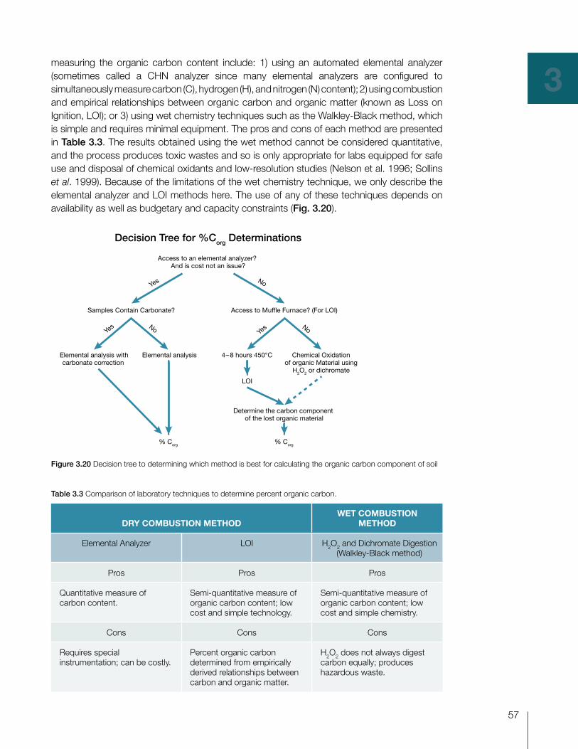
3measuring the organic carbon content include: 1) using an automated elemental analyzer (sometimes called a ChN analyzer since many elemental analyzers are configured to simultaneously measure carbon (C), hydrogen (h), and nitrogen (N) content); 2) using combustion and empirical relationships between organic carbon and organic matter (known as loss on Ignition, lOI); or 3) using wet chemistry techniques such as the Walkley-black method, which is simple and requires minimal equipment. the pros and cons of each method are presented in Table 3.3. the results obtained using the wet method cannot be considered quantitative, and the process produces toxic wastes and so is only appropriate for labs equipped for safe use and disposal of chemical oxidants and low-resolution studies (Nelson et al. 1996; Sollins et al. 1999). because of the limitations of the wet chemistry technique, we only describe the elemental analyzer and lOI methods here. the use of any of these techniques depends on availability as well as budgetary and capacity constraints (Fig. 3.20).

Table 3.3 Comparison of laboratory techniques to determine percent organic carbon.

dry ComBustIon methodWet ComBustIon

method

Elemental Analyzer lOI H2O2 and dichromate digestion (Walkley-black method)

Pros Pros Pros

Quantitative measure of carbon content.

Semi-quantitative measure of organic carbon content; low cost and simple technology.

Semi-quantitative measure of organic carbon content; low cost and simple chemistry.

Cons Cons Cons

requires special instrumentation; can be costly.

Percent organic carbon determined from empirically derived relationships between carbon and organic matter.

H2O2 does not always digest carbon equally; produces hazardous waste.

Decision Tree for %Corg Determinations

Access to an elemental analyzer? And is cost not an issue?

Samples Contain Carbonate? Access to Muffle Furnace? (For LOI)

Elemental analysis withcarbonate correction

% Corg

Determine the carbon component of the lost organic material

Chemical Oxidationof organic Material using

H2O2 or dichromate

4–8 hours 450°C

LOI

Elemental analysis

% Corg

Yes No

YesNo Yes

No

Figure 3.20 decision tree to determining which method is best for calculating the organic carbon component of soil

58

3homogenIzatIon

before the carbon content can be determined, each individual sample/subsample should be homogenized. dried samples are assessed, and any large items, such as stones and twigs are removed, and large clumps are broken up with a spatula. homogenization can be done by manually grinding the dried soils to a powder of consistent particle size using a mortar and pestle or it can be done automatically using a pulverizer or mill (Fig. 3.21). Whichever method is used, it is important to clean the grinding device (e.g., with ethanol) between each soil sample to ensure minimal cross-contamination. the homogenized samples (hereafter called raw soil sample) can then be used for determining the organic and inorganic carbon content.

estImatIng % organIC CarBon usIng an elemental analyzer

For this method dry combustion is used to determine the total carbon (organic and inorganic) for each sample. It is the most suitable method for routine analysis of total carbon, and we recommend use of an elemental analyzer if possible (Sollins et al. 1999). An elemental analyzer is a laboratory instrument used to determine the elemental composition of a sample. the analyzer uses a high temperature induction furnace and either infrared spectroscopy or gas chromatographic separation of gases and thermal conductivity detection to measure the carbon, hydrogen, and nitrogen (as well as other elements) content of the sample.

When using an elemental analyzer, samples are automatically dropped onto the top of a quartz tube maintained at around 1,000 ºC, packed with oxidation reagents and catalysts, and there is a constant flow of helium through the column. When the sample drops onto the top of the column, the helium stream is temporarily enriched with pure oxygen. Flash combustion takes place, producing carbon dioxide, water, and nitrogen. the water is removed using a desiccant, and the CO2 is separated from N2 by gas chromatography. the output of this process is a graph where the amount of carbon is proportional to the area under the CO2 peak (Fig. 3.22), and is reported in units of percent carbon (% C). the instrument is calibrated

A B

C

Figure 3.21 grinding and homogenization of a soil sample. (A) Mortar and pestle, (b) Agate pot in commercially available mill, (C) Agate pot with beads to help pulverize and homogenize the soil sample. (© hilary Kennedy, UWb)

59

3

using an organic compound as a standard, such as acetanilide. the precision of the analysis must be determined using international standards and monitored using an internal standard with a composition close to that of the sample.

If an elemental analyzer is not available, samples can be sent to a commercial laboratory where costs for elemental analysis typically range between $10 and $20 USd per sample. Provided the proper tools are available (microbalance and tin boats), it is possible to save money by weighing out samples and shipping them to a qualified laboratory. In this case, add samples into pre-weighed tin capsule using a spatula, then close and compress using forceps. Weigh the tin capsule with the sample inside, and subtract the weight of the empty tin capsule to determine sample weight. Create a record of where each sample is in the tray, including weights, and ship to the laboratory. the laboratory will need the weight of each sample to calculate the % C in your soil. While awaiting analysis, samples can be stored in a tray inside a desiccator (Fig. 3.23). Ask the laboratory facilities in which you will run the organic carbon analysis for advice before starting to encapsulate the samples (amount of organic carbon needed for robust analyses in their facilities, size of tin capsules needed, etc.). A good option is to run the organic carbon analysis in a few representative samples first and make adjustments as needed before running all of your samples.

Elemental analyzers determine the total carbon content of a sample, including the organic and inorganic carbon. to correct for this, the inorganic carbon content must be determined.

Correcting for Inorganic Carbon Content

Inorganic carbon in the form of carbonates (i.e., calcium carbonate, CaCO3) can be found in coastal soils in the form of shells and/or pieces of coral and is most often associated with seagrass beds. Calcium carbonate may also be present in some mineral-rich soils found beneath layers of peat. (Carbon-neutral sands, silts, and clays will also likely be present in the sediment in varying proportions, but their presence will not affect the analysis of organic carbon.) Calcium carbonate (hereafter referred to as carbonate) contains carbon, but is not included when determining blue carbon stocks, but it will be converted to CO2 in an elemental analyzer, biasing the results.

Nitrogen peak

Carbon peak

Time (sec)

Peak

hei

ght (

mv)

0 50 100 150 200 250 300 350 400 450 500 550 600

Figure 3.22 Chromatogram results from an elemental analyser, showing nitrogen and carbon peaks from combusted sample (© hilary Kennedy, UWb)

60

3

there are two basic methods that correct for the carbonate content of soils.

1) Acidification: this approach is easy, cheap, and requires less sophisticated laboratory equipment. Inorganic carbon is volatilized to CO2 by treating the soil subsample with a strong acid. Inorganic carbon content is estimated from the difference in weight of the subsample before and after treatment. there is a risk that some organic carbon will also be removed using this method leading to a possible under-estimation of organic carbon. reactions with more dilute acids over longer times periods minimizes the loss of organic carbon due to decomposition.

2) Elemental Analyzer: A soil subsample is heated to 500 ºC. At this temperature organic carbon is removed leaving the inorganic carbon in the ash. the inorganic carbon remaining in the ashed subsample is determined using an elemental analyzer.

In both techniques the inorganic carbon content is subtracted from the total carbon (see previous section), what remains it the estimate of organic carbon content.

aCIdIFICatIon

Some protocols for removal of carbonate (e.g., decalcification) use a relatively concentrated acid for short periods of time (Mortlock & Froelich 1989), and others use a more gentle method (Weliky et al. 1983; Pilskaln & Paduan 1992). We recommend the slower and gentler approach to decalcification described here. First, test to see if the sample contains significant quantities of carbonate by taking a subsample (corresponding to the samples used for total carbon analysis), placing it on a glass surface, and adding a few drops of 1N hydrochloric acid (hCl). If carbonate is present, bubbles of CO2 will be generated and the sample will effervesce (Fig. 3.24).

If carbonate is present, weigh out ~ 1 g of your original homogenized soil sample into a 125 ml beaker or a 50 ml glass conical centrifuge tube (the latter is preferred if samples need to be centrifuged to separate solution from soil; see below). dilute hCl to 1N and add enough to the beaker to cover your sample and agitate for 15 minutes by manually

Figure 3.23 Preparing a dried sample for ChN analysis. (A) Extracting a tin capsule to be weighed, (b) After weighing, tin capsule can be placed in clean receptacle, (C) the sample added using a spatula, (d) Forceps are used to close, (E) Compress the tin capsule, and (F) Place the sample in a 96-well plate and store prior to analysis. (© hilary Kennedy, UWb)

A B C

D E F

61

3shaking the sample or by using an ultrasonic bath or probe. both techniques help break up any clumps of soil so that the acid can remove all the inorganic carbon present. the acid is gentle enough to leave the organic matter intact. Allow any effervescence to die down and let samples sit overnight (18–24 hours). Add additional hCl, agitate or sonicate for 15 minutes and check for further effervescence.

If CO2 is no longer being produced (no new outgassing is observed), the carbonate has been removed. Once the soil has settled to the bottom of the beaker/tube the overlying acid can be decanted. If there is a lot of fine-grained soil suspended in solution, centrifuge the samples to separate the solution from the soil and then decant or remove the liquid with a pipette. After the acid has been removed, add distilled water to the sample, swirl, allow the material to settle (or centrifuge), and decant off the water. repeat this washing step two more times. dry at 60 ºC overnight, and weigh the sample.

the mass difference of the sample pre and post acidification is an estimate of calcium carbonate in the sample. however, only 12% of the weight difference can be attributed to carbon (carbon makes up 12% of the molecular weight of calcium carbonate (CaCO3)). thus in order to estimate the amount of inorganic carbon present, the mass of calcium carbonate is multiplied by 0.12. Finally, subtract the inorganic carbon content from the total carbon content of the subsample (from the elemental analysis described in the previous section) to get the organic carbon content of the sample (Table 3.4).

Table 3.4 determining % Inorganic carbon by acidification method

samPle Id

total CarBon Content

(elemental analyzer)

dry mass BeFore aCId

(mg)

dry mass aFter aCId

(mg)

mass oF CarBonate

(mg) InorganIC

CarBon (mg)

InorganIC Content oF

samPle

organIC CarBon

Content oF samPle

A b C d = b – C E = C*0.12 F = (E/b)*100

g = A – F

Example 25% 100 90 10 1.2 1.20% 23.8%

elemental analyzer

take a separate subsample (corresponding to the samples used for organic carbon analysis, ~ 0.5 g) of the dried raw soil, weigh it to the nearest milligram, and place it in a temperature- proof vessel (i.e., ceramic crucible). these samples are then put into a furnace heated to 500 ºC for a minimum of three hours (until a constant weight is reached) to volatilize the organic

Figure 3.24 testing for carbonate. (A) Subsample in a watch glass prior to acidification, (b) pipetting a few drops of weak hCl, (C) subsample effervescing. (© hilary Kennedy, UWb)

A B C

62

3compounds. the weight of the ash remaining is then determined to the nearest milligram. An elemental analyzer is used, following the procedures outlined above, to determine the carbon content of the ash which is assumed to be all inorganic carbon.

Scale the elemental analyzer results by the ratio of ash weight to sample dry weight to get the inorganic carbon content of the original dry sample. then, subtract the inorganic carbon content from the total carbon content of the subsample to get the organic carbon content of the sample (Table 3.5).

Table 3.5 determining % Inorganic carbon by elemental analysis

samPle Id

total CarBon Content

(elemental analyzer)

dry mass BeFore

ashIng (mg)

dry mass aFter

ashIng (mg)

InorganIC CarBon Content oF ashed

samPle (mg)

InorganIC Content oF

samPle

organIC CarBon

Content oF samPle

A b C D E = d*(C/b) F = A – E

Example 25% 500 250 10% 5% 20%

measurIng % CarBon VIa loI analyzer

If the cost of using an elemental analyzer is prohibitive, we recommend using the percent loss on ignition technique (often referred to as % lOI). the initial cost of the equipment needed for % lOI analysis (including a muffle furnace and ceramic crucibles) ranges between $5,000 USd and $10,000 USd. this relatively simple set-up is very durable and can be used for many years, significantly decreasing cost per sample analysis over the long-term.

lOI is a measure of the mass of sample lost (e.g., oxidised and lost as gas, or volatilised) when heated to high temperatures. typically the sample is heated to combustion at 450 ºC for 4–8 hours (heiri et al. 2001). this temperature is used to ensure that only organic (not inorganic) carbon is oxidized.

the % lOI is calculated as follows:

● % loss on Ignition = [(dry mass before combustion (mg) – dry mass after combustion (mg)) / dry mass before combustion (mg)] * 100

Table 3.6 determining % lOI

samPle Id

InItIal mass BeFore

ComBustIon (mg)

FInal mass aFter

ComBustIon (mg)

dIFFerenCe Pre- and

Post- ComBustIon

% loss on IgnItIon

Example 50 40 10 (10/50)*100 = 20

It is important to note that lOI represents the loss of organic matter, which is composed of carbon, hydrogen, nitrogen, oxygen, sulfur, etc. and not solely the loss of organic carbon. thus, a relationship needs to be determined to relate % lOI to % Corg.

Relationship between organic matter and organic carbon: An equation must be constructed that relates organic matter content (% lOI) to the organic carbon content (% Corg) of the same sample. this can be achieved by sending a limited number of samples for organic

63

3carbon analysis using an elemental analyser (see above) and comparing the organic carbon content resulting from that technique to the % lOI results.

If this is not possible, use a value from the literature for a study location/type that most closely resembles your own. the following table (Table 3.7) summarizes examples of the relationships between % lOI and % Corg in mangrove, tidal salt marsh, and seagrass soils. Additional information on the relationships between % lOI and organic carbon in mangrove, tidal salt marsh, and seagrasses can be found in Appendix E. however, there is a large range in the ratios of carbon content (% Corg) to organic matter (% lOI) reported in the scientific literature, making standard ratio values possible sources of error in estimating organic carbon content. therefore, it is good practice to determine the ratio for your particular soils by sending a few samples to a laboratory for elemental analysis. Sending a small number of samples should not be too cost prohibitive and will greatly increase the accuracy of your results.

Table 3.7 relationship between % lOI and % Corg for the different ecosystems. Variability within ecosystems may be due to slight differences in methods used and/or characteristics of the soils.

eCosystem

relatIonshIP

strength (r2)

relatIonshIP BetWeen

% loI and % Corg loCatIon (sourCe)

Mangroves 0.59 % Corg = 0.415 * % lOI + 2.89 Palau (Kaufmann et al. 2011)

Tidal Salt Marshes

0.98 % Corg = 0.47 * % lOI + 0.0008 (% lOI)2 Maine (Johnson et al. in prep)

Tidal Salt Marsh

0.99 % Corg = 0.40 * % lOI + 0.0025 (% lOI)2 North Carolina (Craft et al. 1991)

Seagrasses (% lOI > 0.2)

0.87 % Corg = 0.40 * % lOI – 0.21 global data set (Fourqurean et al. 2012a)

Seagrasses (% lOI > 0.2)

0.96 % Corg = 0.43 * % lOI – 0.33 global data set (Fourqurean et al. 2012a)

While % lOI can be an adequate indicator of organic matter content in many sample types (often defined operationally as % organic matter), it is important to understand the possible limitations of this technique. lOI has been reported to lead to overestimation of organic carbon content in two ways:

1) If a sample containing carbonate (e.g., those underlying seagrass meadows with shoots covered by abundant epiphytes or soils in the region of coral reefs) is heated above 500 ºC, loss of water and CO2 derived from CaCO3 may also be driven off (hirota & Szyper 1975; leong & tanner 1999).

2) In soils containing > 11% clay minerals, a significant amount of structural water (that is not lost by heating at 60 ºC) may be driven off during heating at this higher temperature (barillé-boyer et al. 2003).

In both cases, the organic carbon content could be overestimated due to the fact that the % lOI could reflect a loss of organic matter, inorganic carbon, and structural water contained within the sample. A reduction in the error arising from % lOI may be achieved by determining and correcting for the inorganic content (see section below on correcting for inorganic carbon).

64

3CalCulatIng total soIl CarBon stoCKthe total soil carbon stock within a project area is determined by the amount of carbon within a defined area and soil depth. to calculate the total soil carbon for your project area you will need the following information:

● Soil depth,

● Subsample depth and interval,

● dry bulk density, and

● % Organic carbon.

the total carbon stock in a project area can be determined as follows:

Step 1: For each interval of the core sampled/analyzed, calculate the soil organic carbon density as follows:

Soil carbon density (g/cm3) = dry bulk density (g/cm3) * (% Corg/100).

Step 2: Calculate the amount of carbon in the various sections of core sampled by multiplying each soil carbon density value obtained in step 1 by the thickness of the sample interval (cm):

Amount carbon in core section (g/cm3) = Soil carbon density (g/cm3) * thickness interval (cm).

Step 3: Sum the amount of carbon in core sections over the recommended total sampling depth (1 m at a minimum). It is critical that the total sampling depth be included in your report.

Core #1 summed = Amount carbon in core section A (g/cm3) + Amount carbon in core section b (g/cm3) + Amount carbon in core section C (g/cm3) + …. all the samples from a single core.

*the entire core needs to be included in this calculation. If subsamples were taken along the core (Fig 3.11), sum the amount of carbon in each of the sections and then sum over the total depth sampled to get the total carbon stock.

Step 4: Convert the total core carbon from step 3 into the units commonly used in carbon stock assessment (MgC/hectare-cm) using the following unit conversion factors (there are 1,000,000 g per Mg (megagram), and 100,000,000 cm2 per hectare):

total core carbon (MgC/hectare-cm) = Summed core carbon (g/cm3) * (1 Mg/1,000,000 g) * (100,000,000 cm2/1 hectare).

the unit here is Mg C/hectare (for the top 1 m soil), and is a typical unit used in carbon stock assessment.

REPEAT FOR EACH CORE

Step 5: determine the average amount of carbon in a stratum for given depth and calculate the associated standard deviation to determine variability/error.

Average carbon in a core = Carbon content for core #1 (determined in step 4) + Carbon content for core #2 + Carbon content for core #3+…. n) / n.

65

3Standard deviation (σ) determines how closely the data are clustered about the mean, and is calculated as follows:

Core Standard Deviation (σ) = [ (X1 − X) 2 + (X2 − X) 2 + … (Xn − X) 2 ] 1/2

(N−1)● X = average carbon in a core● X1 = individual result for core #1, in MgC/hectare; X2 = individual result for core

#2, in MgC/hectare, etc.,● N = total number of results.

Step 6: to obtain the total amount of carbon in the ecosystem, multiply the average carbon value (MgC/hectare) for each core obtained in step 5 above by the area of each stratum (in hectares) to determine MgC for each stratum, and then sum the MgC values for each stratum to determine the total soil carbon stock.

Again, it is critical to note the total depth of the soil cores. thus, the final unit for soil carbon stock in each project strata will be MgC over a specific depth interval (usually, but not always 1m).

total organic carbon in a project area (MgC) = (average core carbon from Statum A (MgC/hectare) * area Statum A (hectares)) + (average core carbon from Statum b (MgC/hectare) * area Statum b (hectares) + …

Step 7: to report a value for the variability/error associated with these measurements, calculate the total uncertainty in the data. First, calculate the standard deviation of the average Mg C for each stratum. [Multiply the standard deviation carbon value (MgC/hectare) for each core determined in step 5 (above) by the area of each stratum (in hectares).] then propagate the uncertainty through the calculations by combining the standard deviations of the average MgC for each stratum as follows:

σΤ = σA2+ σb2+...σN2

● Where σΤ = the total variability associated with the measurements,● σA = standard deviation of the core average MgC for stratum A * area of stratum,● σb = standard deviation of the core average MgC for stratum b * area of

stratum, and● σN = standard deviation of the core average MgC for remaining stratum * area of

each individual stratum.

this approach can be used when adding average values, as is done when combining the data from the individual strata.

Step 8: the final soil carbon stock will be presented in an average value ± the total uncertainty. Alternatively, a minimum and maximum carbon stock can be presented by multiplying by the project area by the minimum and maximum carbon densities.

total organic carbon in a project area (calculated in Step 6) ± the standard deviation (calculated in Step 7)

Equations and examples are provided in Appendices b and C.

66

3QuICK guIde

Step 1: Determine Soil Depth

• Measure depth to parent materials, bedrock, or coral sands.

Step 2: Soil Coring

• Choose soil coring device based on type of soil and degree to which the soil is saturated with water.• Steadily insert the coring device until the top of the sampler is level with the soil surface.• Once at depth, twist the coring device to cut through any remaining fine roots, measure the length

of pipe outside the sediments and the length of empty pipe, and seal the top end (the vacuum will prevent the loss of the sample).

• gently pull the coring device out of the soil while continuing to twist as it is being extracted. this twisting assists in retrieving a complete soil sample.

• In the case of seagrasses, the coring device must often be removed from the soil using a winch.• It is imperative to note the total depth and any compression.

Step 3a: Sampling an Entire Soil Core (if this is not feasible subsampling can be done, next section)

• It is best to sample the entire depth of the soil core; however, this may not always be possible or practical.

• It is imperative to record subsample depth, depth interval and volume.

Step 3b: Subsampling a Soil Core

• Samples should be collected from homogenized sample intervals or from the approximate mid-point of each desired depth range.

Step 4: Archiving samples

• the proper labelling of the cores and samples in the field is essential to avoid confusion and common mistakes in sample identification.

• Each sample/subsample should be labelled with at least a core Id, sample depth, and depth interval.

Step 5: Storing samples

• to minimize decomposition of organic matter, samples should be kept cold (at 4 °C) and, if possible, frozen within 24 hours of collection.

Step 6: Determining Dry Bulk Density (g/cm3)

• Calculate the volume of soil sampled using the equation (cm3)• determine the dry weight.• Calculate dry bulk density by dividing the mass of dried soil by the volume of soil sampled (g/cm3).

Step 7: Determine Organic Carbon Content

• decide which techniques to use based on desired result, capacity, and budgetary constraints.• determine inorganic carbon content.• determine organic carbon content.

Step 8: Calculate Total Soil Carbon Stock

• If you subsampled the core, you will need to determine the amount of carbon per cm3 of the core and then multiply that by the length of the sample interval, then add all the intervals together to determine the total carbon /area represented in the core.

• You must include the variability associated with the measurements and the total soil depth assessed when reporting results.