Field-Scale Measurement of Groundwater Profiles in a ...inside.mines.edu/~psanti/paper_pdfs/Cook Field GW profiles.pdf · Field-Scale Measurement of Groundwater Profiles in a

Field-Scale Measurement of Groundwater Profiles in a

Drained Slope

DIANA I. COOK

PAUL M. SANTI

JERRY D. HIGGINS

Department of Geology and Geological Engineering, Colorado School of Mines,1516 Illinois Street, Golden, CO 80401

RICHARD D. SHORT

Blackhawk Geologic Hazard Abatement District, 4125 Blackhawk Plaza Circle,Danville, CA 94506

Key Terms: Groundwater, Slope-Stability, Horizon-tal, Drains, Field-Measurement

ABSTRACT

In 2003, Crenshaw and Santi developed a method forcalculating average piezometric heads between horizon-tal drains in a slope. The method relies on drain flowrates, slope geometry, and soil hydraulic conductivity.The corrugated shape of groundwater profiles betweendrains and the departure of the groundwater surfacefrom the drain near its uphill end were verified usinglaboratory-scale physical and computer modeling. In2007, a study was conducted seeking to confirm thesefindings using field-scale modeling. The test site con-sists of a 2H:1V (2 horizontal : 1 vertical), 30 3 12 ft(9.1 3 3.7 m) concrete slope representing low-perme-ability bedrock. Five perforated pipes embedded in theconcrete are used to simulate base-flow recharge. Theconcrete was covered with a lean clay, and two wickdrains were installed at a spacing of 8 ft (2.4 m). Fiftystandpipe piezometers were installed to measure ground-water profiles between and along drains. Measurementswere taken during recharge and drawdown events. Thetest was repeated with a clayey sand. Test resultsgenerally confirm the findings of Crenshaw and Santi,with some localized variations in groundwater profiles.The variations are most likely due to factors such asheterogeneous soil properties, the development ofpreferential pathways, boundary effects, etc. Field-testing also yielded additional information about thebehavior of drained slopes that may be useful for futureslope-stability projects. As a result of this research,recommendations for using Crenshaw and Santi’smethod to estimate piezometric heads between short,high-angle sub-horizontal drains in shallow landslides foruse in slope-stability analyses are provided.

INTRODUCTION

Landslides, debris flows, and mudflows are com-mon geologic hazards throughout the world. One ofthe most common preventative and remedial tech-niques used to reduce the likelihood and magnitude ofthe occurrence of these hazards is groundwaterdrainage. However, design and installation of hori-zontal drains is still based very much on experience,observation, and local practice and not on standard-ized engineering techniques (Cook et al., in press).

This article specifically addresses a commonassumption in slope-stability modeling, namely, thatthe groundwater profile stays fairly level across theslope; that is, perpendicular to the slope angle.Laboratory-scale physical modeling and computermodeling have shown that this is not the case whenhorizontal drains have been installed. The ground-water is lowest at the drain location and rises betweendrains (Figure 1). Accounting for the remedialdrainage effect on a three-dimensional (3-D) ground-water profile in a slope-stability model can make adifference in the safety factor by as much as 10percent (Santi et al., 2003). A potential method existsfor estimating the drainage effect on piezometricheads within remedially-engineered slopes for use instability analyses (Crenshaw, 2003; Crenshaw andSanti, 2004), but was not previously verified withfield-scale testing.

In an effort to verify this potential method forestimating groundwater levels in drained slopes, twosoil slopes were constructed at the BlackhawkGeologic Hazard Abatement District (GHAD) testsite near Danville, California, during the summermonths of May, June, and July in 2007. The twoslopes, a sandy clay (CL) slope and a clayey sand (SC)slope, built consecutively, were each outfitted with

Environmental & Engineering Geoscience, Vol. XIV, No. 3, August 2008, pp. 167–182 167

two horizontal wick drains and 50 piezometers andwere built above perforated water pipes used tosimulate recharge. The materials and geometry usedin the construction of the slopes were estimated to berepresentative of shallow landslides common to theGHAD and to other hill-slope areas in California,which are characterized by homogenous to semi-homogeneous soils or weak-rock slope materials thatare largely unaffected by the presence of rock joints.The constructed slopes were used to observe theeffects of recharge and drainage on groundwaterprofiles within shallow soil slopes to improve thedesign and installation of slope-drainage projects.The purpose of this article is to document the testingprogram and provide a comparison of field-measuredgroundwater levels and profile shapes with thosepredicted using Crenshaw and Santi’s method. Inaddition, the article provides recommendations forusing the method to estimate piezometric headsbetween short, high-angle (20–25 degree inclinationsfrom the horizontal) sub-horizontal drains in shallowlandslides for use in slope-stability analyses.

BACKGROUND

In general, Crenshaw and Santi’s (Crenshaw, 2003;Crenshaw and Santi, 2004) work showed the ground-water surface in a drained slope to be corrugated inshape, with lows along the drains and highs betweenthem (Figure 1). In the upper part of the slope, alongthe back half of the drains, the groundwater surfacediverges from the drains, rising above them (Fig-ure 2). Crenshaw and Santi’s work also established amethod for averaging a 3-D groundwater surface to

create a representative two-dimensional (2-D)groundwater profile for use in slope-stability pro-grams that require a 2-D cross section of a slope.Because the field tests and water-level predictionscovered in this article were based on these methods, asummary of the physical testing program employedby Crenshaw and Santi is included below.

Crenshaw and Santi (Crenshaw, 2003; Crenshawand Santi, 2004) used three laboratory-scale physicaltests and computer modeling to analyze variousrecharge scenarios that could be expected to occur inthe field based on the hydraulic conductivity of the soilcomposing a slide mass. The tests showed that thegroundwater profile varied primarily according toaverage hydraulic conductivity. The profiles (Figure 2)were grouped based on whether the groundwaterprofile diverged upward from the drain at its end(L100), or at some location along the drain correspond-ing to a percentage of its total length (Lc). Although Lcis important in Crenshaw and Santi’s calculations todevelop correction factors, these correction factors arenot applicable for the conditions tested in this project,so Lc is not used except as reference to the location ofgroundwater divergences from the drains.

Crenshaw and Santi’s three laboratory-scale testsvaried the source of the recharge and the recharge rate.The first test simulated a rainfall event by allowingrecharge from above and behind the drain system. Thesurface of the soil was pre-saturated, and steady statewas established, denoted by constant heads in the testpiezometers. Initial water-profile measurements wererecorded, after which the water source was turned off.Measurements of the piezometric heads and flow rateswere then recorded during drawdown. Drawdown was

Figure 1. Shape of groundwater surface within a drain field. Note troughs corresponding to drain locations and ridges located betweendrains (Crenshaw and Santi, 2004).

Cook, Santi, Higgins, and Short

168 Environmental & Engineering Geoscience, Vol. XIV, No. 3, August 2008, pp. 167–182

sustained for about 1 hour for sand soils and360 hours for clays and silts. The second test simulateda variable groundwater recharge source by allowingrecharge only from behind the drain system. This wasaccomplished by the addition of a reservoir near thewater-entry source in the test container. After steadystate was established, in the same manner as the firsttest, the water source was turned off and measurementsof the piezometric heads were recorded duringdrawdown to compare the changing groundwaterprofiles with the short-term changes in recharge rate.Drawdown was sustained for about 1 hour for sandsoils and 96 hours for clays and silts. This simulationrepresented periodic high-precipitation events, springsnow thaws, or recharge due to agricultural irrigation.The third test simulated recharge from a constantgroundwater source by allowing water to enterthrough a constant-head reservoir behind the drainsystem. To keep the recharge rate from varying, thetest was performed in a sand soil so that the hydraulicconductivity would be high enough to keep the waterfrom ponding in the test container. Once steady statewas established, denoted by a constant volumetric flowfrom the drain, piezometric heads and the dischargeflow rates from the drains were recorded. Because thisthird test was specifically for groundwater profilesunder constant recharge, no drawdown measurementswere recorded. Similar tests were repeated in the field,as described in the next section, in an effort to confirmthe findings of the original work at a larger and morerealistic scale.

METHODS

Description of Test Site

The test site consists of a 30 3 12 ft (9.1 3 3.7 m)concrete slab, which roughly approximates the

bedrock surface typical of Quaternary-aged residualslopes in the area, constructed on a hill side at a2H:1V (2 horizontal : 1 vertical) slope. In order tosimulate the effects of excess infiltrated precipitationand groundwater seepage, the concrete slab wasoutfitted with both surficial and sub-surface infiltra-tion systems. Five parallel, 1-in. (25.4-mm) diameter,perforated polyvinyl chloride (PVC) pipes were laidinto troughs mechanically chipped into the concrete.Non-perforated PVC was used to extend the pipes tothe top of the slope, where a junction box was used toaccommodate a separate valve for each pipe. A maininfiltration line providing water to the pipes wasoutfitted with a water meter to provide flow dataduring testing (Collins, 2006). The main infiltrationline was also outfitted with a connection for a hose toprovide surface soaking and infiltration. Soil com-pacted on top of the slab simulates residual soildeveloped on top of the bedrock.

Test Slope Design

The constructed soil slopes enabled water-levelmeasurements to be taken both between and alongdrains in a hillside. Thus, in addition to two sub-horizontal wick drains, rolled and tied with electricalties to simulate drain pipes and spaced 8 ft (2.4 m)apart, the slopes included 50 piezometers (Figure 3).Three rows of 12 piezometers, spaced laterally at 1 ft(0.3 m) intervals, were located 5 ft (1.5 m), 10 ft(3.0 m), and 20 ft (6.1 m) from the top of the slopesto measure groundwater profiles between drains atdifferent intervals in the slopes. Additional piezom-eters were placed at 2 ft (0.6 m) intervals along thedrains; four between the second and third lateral rowsand three after the third lateral row. These additionalpiezometers enabled monitoring of the groundwaterzone paralleling each side of each drain, where the

Figure 2. Groundwater profile classifications for horizontal drains, showing the location of drain contact, Lc (modified from Crenshaw,2003).

Groundwater Profiles


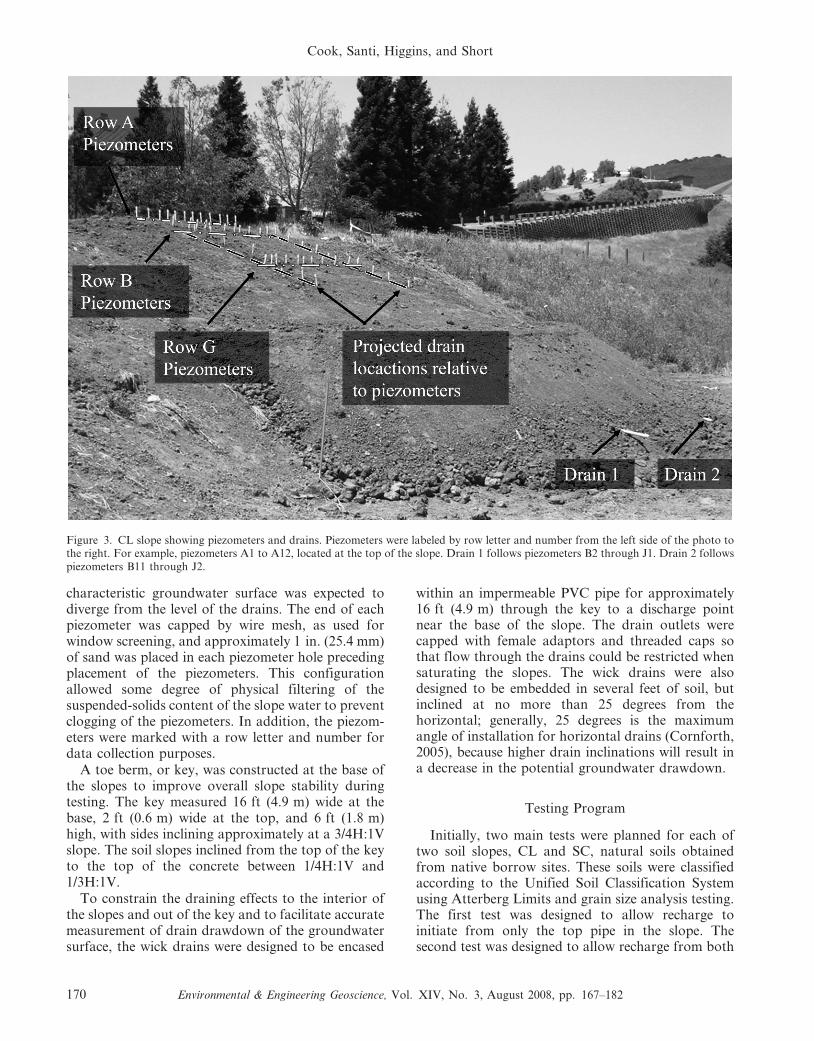
characteristic groundwater surface was expected todiverge from the level of the drains. The end of eachpiezometer was capped by wire mesh, as used forwindow screening, and approximately 1 in. (25.4 mm)of sand was placed in each piezometer hole precedingplacement of the piezometers. This configurationallowed some degree of physical filtering of thesuspended-solids content of the slope water to preventclogging of the piezometers. In addition, the piezom-eters were marked with a row letter and number fordata collection purposes.

A toe berm, or key, was constructed at the base ofthe slopes to improve overall slope stability duringtesting. The key measured 16 ft (4.9 m) wide at thebase, 2 ft (0.6 m) wide at the top, and 6 ft (1.8 m)high, with sides inclining approximately at a 3/4H:1Vslope. The soil slopes inclined from the top of the keyto the top of the concrete between 1/4H:1V and1/3H:1V.

To constrain the draining effects to the interior ofthe slopes and out of the key and to facilitate accuratemeasurement of drain drawdown of the groundwatersurface, the wick drains were designed to be encased

within an impermeable PVC pipe for approximately16 ft (4.9 m) through the key to a discharge pointnear the base of the slope. The drain outlets werecapped with female adaptors and threaded caps sothat flow through the drains could be restricted whensaturating the slopes. The wick drains were alsodesigned to be embedded in several feet of soil, butinclined at no more than 25 degrees from thehorizontal; generally, 25 degrees is the maximumangle of installation for horizontal drains (Cornforth,2005), because higher drain inclinations will result ina decrease in the potential groundwater drawdown.

Testing Program

Initially, two main tests were planned for each oftwo soil slopes, CL and SC, natural soils obtainedfrom native borrow sites. These soils were classifiedaccording to the Unified Soil Classification Systemusing Atterberg Limits and grain size analysis testing.The first test was designed to allow recharge toinitiate from only the top pipe in the slope. Thesecond test was designed to allow recharge from both

Figure 3. CL slope showing piezometers and drains. Piezometers were labeled by row letter and number from the left side of the photo tothe right. For example, piezometers A1 to A12, located at the top of the slope. Drain 1 follows piezometers B2 through J1. Drain 2 followspiezometers B11 through J2.



the top pipe in the slope and from a sprinkler abovethe slope to simulate recharge from a single, worst-case, sustained rainfall event. In addition, threedifferent recharge rates were tentatively planned foreach test, depending on the results collected from theinitial recharge rates used.

In general, for the first set of tests, the drainswere initially capped during slope saturation. Theslopes were saturated using all five recharge pipes,but not all at once or continuously. The piezo-metric head was allowed to rise approximately3.5 ft (1.1 m) and 4 ft (1.2 m) above the concreteand about 1.5 ft (0.5 m) and 2 ft (0.6 m) abovethe level of the drains in the CL slope and theSC slope, respectively. These heads were verifiedby lowering the tip of an electronic water-levelindicator into the piezometers on the slope. Afterthe slopes became saturated, the drains were un-capped and recharge continued from one or moreof the top three pipes, depending on seepage patterns,so that the water was not allowed to seep up toand over the surface of the slope. The total rateof inflow was monitored and compared to theoutflows of the two drains, which were measuredwith a bucket and a stopwatch. Steady state (definedas inflow 5 outflow with relatively constant heads inthe slope) was established in the CL slope atapproximately 0.013 gal/min (0.82 cm3/s). Steadystate was established so that drawdown could beinitiated with the maximum head, between drains, forthe recharge rate used. The time to reach steady statealso allowed the slope-mass water to take on itspreferred shape relative to the location of the drains.The water source was then turned off, and thechanges in the draining groundwater profile wererecorded over periodic increments using an electronicwater-level indicator. For the CL soil, drawdown wasmeasured at 2, 6, 14, 30, 54, and 102 hours after thewater source was turned off.

For the SC soil, the slope was initially saturatedand an attempt to reach steady state was made.Steady state was not reached due to severe seepageissues. The slope was saturated again the followingday, but because this second attempt to reach steadystate also failed, drawdown was initiated regardless.Total drain outflow before the water source was shutoff was approximately 0.42 gal/min (26.3 cm3/s).Drawdown water levels in the SC slope weremeasured at 1, 3, 7, and 15 hours after the watersource was turned off.

The project schedule originally allowed for a weekof construction on the CL slope and approximately 2weeks of testing before a scheduled week-long hiatusin the program. As construction took twice as long asanticipated, the testing for the CL slope started with a

preliminary saturation phase to gage how well the restof the testing would proceed. Water-level data werecollected for this preliminary saturation phase al-though there was not enough time for a full test. Afull test was performed after the hiatus.

The second test was not performed for either slopebecause of seepage issues at even very low rechargerates (less than 0.015 gal/min [0.95 cm3/s] for the CLslope, and less than 0.10 gal/min [6.3 cm3/s] for the SCslope). With seepage issuing from the surface of theslopes, the infiltration from surface sprinklers wouldhave been indeterminate, so this phase of the experi-ment was eliminated. The surficial seepage at such lowrecharge rates also made it impossible to allow fortesting using significantly higher recharge rates.

Total testing time for the CL soil, includingpreliminary saturation (one full test) and an attemptto reach steady state at a recharge rate greater thanthat used for the first test, was approximately 14 days.Total testing time for the SC soil, including slopesaturation and both attempts to reach steady state,was about 4 days.

Calculated vs. Actual Piezometric Heads

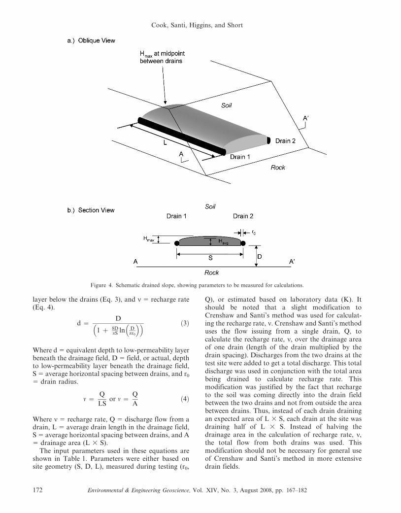
Equations established by Crenshaw and Santi(Crenshaw, 2003; Crenshaw and Santi, 2004) wereused to calculate piezometric heads for both the CLand SC soil slopes. These calculated heads are takenfrom the location of drain contact (Figure 4) andrepresent an average maximum head (Hmax) and anoverall average head (Havg) midway between thedrains. Thus the calculated heads are averages for thewhole drain field. The equations used for thecalculations are as follows.

Hmax ~

ffiffiffiffiv

K

r ffiffiffiffiffiffiffiffiffiffiffiffiffiffiffiffiffiffiS2

4{ x2

r !{ d ð1Þ

Where Hmax 5 piezometric head above the drains andat the midpoint between two drains, x 5 horizontaldistance from the midpoint of two drains, (x 5 0 forHmax), K 5 hydraulic conductivity, S 5 averagehorizontal spacing between drains, d 5 equivalentdepth to low-permeability layer below the drains(Eq. 3), and n 5 recharge rate (Eq. 4).

Havg estimate ~ pS

8

ffiffiffiffiv

K

r� �{ d ð2Þ

Where Havg estimate 5 average piezometric head abovethe drains in a drained slope, K 5 hydraulicconductivity, S 5 average horizontal spacing betweendrains, d 5 equivalent depth to low-permeability



layer below the drains (Eq. 3), and n 5 recharge rate(Eq. 4).

d ~D

1 z 8DpS

ln Dpr0

� �� ð3Þ

Where d 5 equivalent depth to low-permeability layerbeneath the drainage field, D 5 field, or actual, depthto low-permeability layer beneath the drainage field,S 5 average horizontal spacing between drains, and r0

5 drain radius.

n ~Q

LSor n ~

Q

Að4Þ

Where n 5 recharge rate, Q 5 discharge flow from adrain, L 5 average drain length in the drainage field,S 5 average horizontal spacing between drains, and A5 drainage area (L 3 S).

The input parameters used in these equations areshown in Table 1. Parameters were either based onsite geometry (S, D, L), measured during testing (r0,

Q), or estimated based on laboratory data (K). Itshould be noted that a slight modification toCrenshaw and Santi’s method was used for calculat-ing the recharge rate, n. Crenshaw and Santi’s methoduses the flow issuing from a single drain, Q, tocalculate the recharge rate, n, over the drainage areaof one drain (length of the drain multiplied by thedrain spacing). Discharges from the two drains at thetest site were added to get a total discharge. This totaldischarge was used in conjunction with the total areabeing drained to calculate recharge rate. Thismodification was justified by the fact that rechargeto the soil was coming directly into the drain fieldbetween the two drains and not from outside the areabetween drains. Thus, instead of each drain drainingan expected area of L 3 S, each drain at the site wasdraining half of L 3 S. Instead of halving thedrainage area in the calculation of recharge rate, n,the total flow from both drains was used. Thismodification should not be necessary for general useof Crenshaw and Santi’s method in more extensivedrain fields.

Figure 4. Schematic drained slope, showing parameters to be measured for calculations.



It should also be noted that Crenshaw and Santi’smethod provides for a piezometric head correctionfactor to account for variable recharge rates in slopeswith specific groundwater profile characteristics. Inessence, the correction factor allows specific heads tobe calculated along the profile near the back end of thedrains, where the groundwater rises above the esti-mated Havg. No correction factor was employed for thecalculations carried out, mainly because, for this sitegeometry, the groundwater profiles do not rise at theback of the drain; instead the drains are dry along theend where they terminate in the slope. Thus, onlyaverage piezometric heads can currently be calculatedfor slopes with geometries similar to the field site.

After calculation of the average piezometric heads,a comparison was made to values measured fromgroundwater profiles along piezometer Row G. RowG was chosen based on water-level data, whichindicated that it was the location in the slope closestto the location of drain contact (Lc) and thus thelocation closest to the heads calculated using Cren-shaw and Santi’s method. The groundwater profilesused for the CL soil corresponded to steady state, orequilibrium, and drawdown at 6 hours, whereas thegroundwater profiles used for the SC soil correspond-ed to 1 hour of drawdown, as steady state was notreached, and drawdown at 3 hours. In general, thewater-level values measured in the eight piezometerslocated between the drains were used to estimate theaverage piezometric heads above the level of thedrains. However, the CL steady state profile forpiezometer Row G contained an anomalously highvalue near Drain 2. This value was not used as themaximum nor was it used in estimating the averagepiezometric head between drains.

RESULTS

The slope test results and piezometric headcalculations are summarized below and in Figures 5

through 12. It should be noted that a few profileshave data points missing for some of the piezometers.No water was present in these piezometers, mostlikely as a result of clogging.

Groundwater Profiles in the CL Slope

Cross sections in the CL slope show a general risingof the groundwater between drains with some localizedperturbations (Figure 5). In addition, the measuredgroundwater profiles were, in general, initially higheron the right side of the slope (right side of Figure 5),toward the front of the recharge pipes, and lower on theleft (left side of Figure 5), near the end of the rechargepipes. This is especially apparent in Row G in Figure 5.As the water in the saturated slope was allowed toequilibrate over time, the discrepancy between thewater levels decreased. Figure 5 also shows thatlocalized perturbations present in the slope at equilib-rium, after the hiatus in testing, exhibited greater reliefthan the perturbations present in the slope during initialsaturation, particularly lower in the slope, near thevicinity of Row G. During drawdown, the waterprofiles between drains along Rows B and G changedshape slowly and by very little; the mid-point betweendrains stayed high compared to the areas around thedrains as drawdown proceeded. As observed in crosssections along the drains (Figure 6), small pockets ofperched water formed above Drains 1 and 2 duringinitial saturation, but equilibrated over time; thepockets flowed downhill and, because of the presenceof the low permeability key, the slope-mass waterstarted to back-up into the upper slope, creating largepockets of perched water near the front half of thedrains. Along the drains, drawdown proceeded fromback (near the slope crown) to front (near the slope toe).

Groundwater Profiles in the SC Slope

In general, cross sections between drains in the SCslope (Figure 7) show the same trends observed in the

Table 1. Input Parameters Used To Calculate Crenshaw and Santi Piezometric Heads (1 ft 5 0.3 m).

Slope Soil Type and Test PhaseCL, Steady

StateCL, 6 HoursDrawdown

SC, 1 HourDrawdown

SC, 3 HoursDrawdown

Radius of drain, r0 (ft) 0.042 0.042 0.042 0.042Field depth to low-permeability layer, D (ft) 1.87 1.87 1.78 1.78Equivalent depth to low-permeability layer, d (ft) 0.72 0.72 0.72 0.72Flow from drains, Q (ft3/s) 2.90E-05 2.23E-05 3.34E-04 1.67E-04Drain spacing, S (ft) 8 8 8 8Length of drains, L (ft) 21.7 21.7 21.7 21.7Drainage area, A (ft2) 173.60 173.60 173.60 173.60Recharge rate, n (ft/s) 1.67E-07 1.28E-07 1.93E-06 9.63E-07Hydraulic conductivity, K (ft/s) 4.27E-07 4.27E-07 4.27E-06 4.27E-06

CL 5 sandy clay; SC 5 clayey sand.



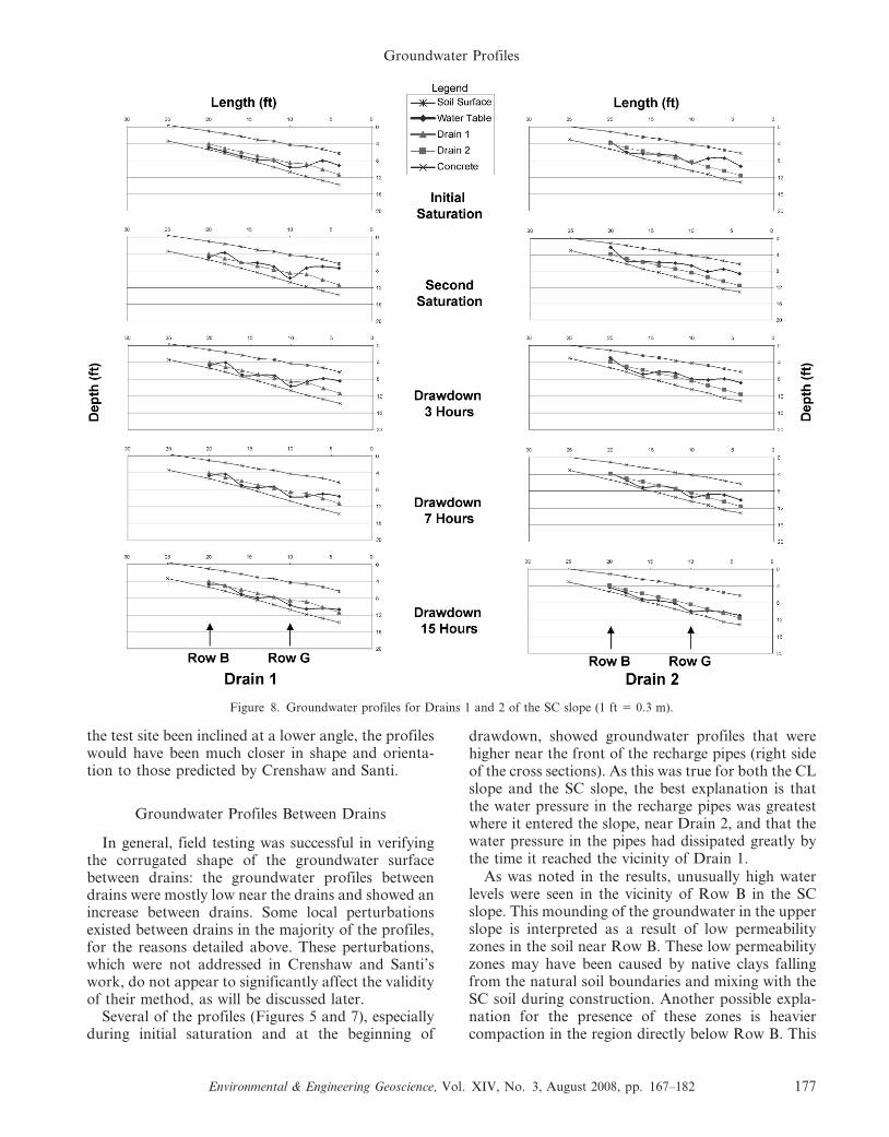
CL slope: a rising water surface between drains, higherwater levels toward the front of the recharge pipes,exaggerated perturbations after a second saturationphase (this time mainly in Row B), faster drawdown inthe vicinity of the drains, and slower drawdown nearthe mid-point between drains. Cross sections alongdrains in the SC slope were also, in general, similar tothose for the CL slope (Figure 8). The perturbationsalong the drains increased in number and severitybetween the initial saturation of the slope and thesecond attempt to saturate the slope and bring it tosteady state. In addition, large pockets of perchedwater similar to those along the drains in the CL slopealso formed in the SC slope near the key boundary,although the pockets in the SC slope tended to belarger as a result of the higher permeability of theslope. Drawdown along the drains in the SC slope alsoproceeded from the back end of the water pockettoward the front of the drain, near the slope toe.

It should be noted that during the first attempt toreach steady state in the SC slope, a rise in the waterlevels in Row B was observed even though the drainswere open and the recharge rate was very low. Duringthe same period, Row G water levels receded. Whilesaturating the slope the following day, Row B againexhibited unusually high water levels, especiallycompared to Row G (second saturation phase inFigure 7). These occurrences corresponded to severesurface seepage, which, as mentioned previously,proved especially difficult to control on the SC slope.

Results for Calculated vs. Field-MeasuredPiezometric Heads

Calculated heads and heads measured in Row G ofthe soil slopes show good agreement. Values calcu-lated for the CL slope, shown in Table 2, vary by less

Figure 5. Groundwater profiles for Rows B and G of the CL slope (1 ft 5 0.3 m).



than 0.3 ft (0.09 m) from heads measured in the field.Values calculated for the SC slope, shown in Table 3,vary by less than 0.35 ft (0.11 m) from headsmeasured in the field. A comparison of the calculatedand field-measured results can also be seen inFigures 9 and 10 for the CL slope and Figures 11and 12 for the SC slope.

ANALYSIS AND DISCUSSION

Factors Influencing Water Levels

Measured water levels appeared to exhibit theeffects of factors beyond the release of pressure headthrough the wick drains. These factors may includesome or all of the following:

N anisotropy/macropore flow

N effects of inconsistent compactionN effects of shallow bedrockN effects of vertical head distributionN boundary effects of toe berm and sidesN effects of drain steepness

A more detailed description of how each of thesefactors may have influenced measured water levels isincluded below.

The deviations in the groundwater profiles werelikely caused by several of the above factors. Theslope soils were heterogeneous and therefore pos-sessed some inherent anisotropy, as would the naturalslopes they were intended to model. In addition,compaction around the piezometers was madedifficult by their close proximity to each other, whichcompounded the anisotropy. Macropores appear tohave developed both during the saturation phases of

Figure 6. Groundwater profiles for Drains 1 and 2 of the CL slope (1 ft 5 0.3 m).



testing and, especially in the case of the CL slope,during periods where the slope was allowed to dryand crack. The shallow bedrock and relatively thinsoil in the slopes most likely contributed to thedevelopment of macropores and the ease with whichthe saturation front moved toward the surface, which,on many occasions, resulted in free-flow, spring-type,break-outs of surface seepage. Another possiblecontributing factor to the presence of local distur-bances in the groundwater profiles is the effect of avariable vertical-head distribution in the slope. As thepiezometer tips were not installed at the same depth,because of the presence of the concrete slope, thesaturation front may not have spread equally to allpiezometers. Whereas these factors may have de-creased the accuracy of the results of this study, thesame factors would also affect natural slopes, so thesefield tests are quite realistic.

The toe berm, or key, was built to be less permeablethan the rest of the slope, resulting in a boundaryeffect that caused the water in both soil slopes tomound at the intersection of the key and the slope.The sides of the slope, however, were left in theirnatural state and appear to have had a slight influenceon the groundwater profiles at the edges of the slopesonly when the water levels in the slope dropped to thelevel of the drains. Finally, the steepness of the drainsresulted in a portion of their length remaining dryeven while they were draining effectively. Also, thesteepness of the drains resulted in groundwaterprofiles along the drains that do not match thosepredicted by Crenshaw and Santi: the water profilesdo not rise at the back of the slope, but instead tendto be dry at the back of the slope. Because Crenshawand Santi’s results were based on drains oriented closeto the horizontal, it is expected that, had the drains at

Figure 7. Groundwater profiles for Rows B and G of the SC slope (1 ft 5 0.3 m).



the test site been inclined at a lower angle, the profileswould have been much closer in shape and orienta-tion to those predicted by Crenshaw and Santi.

Groundwater Profiles Between Drains

In general, field testing was successful in verifyingthe corrugated shape of the groundwater surfacebetween drains: the groundwater profiles betweendrains were mostly low near the drains and showed anincrease between drains. Some local perturbationsexisted between drains in the majority of the profiles,for the reasons detailed above. These perturbations,which were not addressed in Crenshaw and Santi’swork, do not appear to significantly affect the validityof their method, as will be discussed later.

Several of the profiles (Figures 5 and 7), especiallyduring initial saturation and at the beginning of

drawdown, showed groundwater profiles that werehigher near the front of the recharge pipes (right sideof the cross sections). As this was true for both the CLslope and the SC slope, the best explanation is thatthe water pressure in the recharge pipes was greatestwhere it entered the slope, near Drain 2, and that thewater pressure in the pipes had dissipated greatly bythe time it reached the vicinity of Drain 1.

As was noted in the results, unusually high waterlevels were seen in the vicinity of Row B in the SCslope. This mounding of the groundwater in the upperslope is interpreted as a result of low permeabilityzones in the soil near Row B. These low permeabilityzones may have been caused by native clays fallingfrom the natural soil boundaries and mixing with theSC soil during construction. Another possible expla-nation for the presence of these zones is heaviercompaction in the region directly below Row B. This

Figure 8. Groundwater profiles for Drains 1 and 2 of the SC slope (1 ft 5 0.3 m).



area may have received heavier compaction thansome of the other areas adjacent to piezometersbecause, due to the geometry of the test site(Figure 3), it was more accessible and not as tightlybounded by piezometers.

In the vicinity of Drain 1, the groundwater surfacewas often located below the level of the drain. This wasalso true for Drain 2, although only after the rechargepipes were closed and drawdown was initiated. Thiscan be explained by both the steepness of the drainsand the effects of seepage at the side boundaries. Thesteepness of the drains most likely plays a larger role,because the groundwater profiles generally rise slightlyfrom below the drains toward the side boundaries (seeFigure 7, drawdown at 3 hours). The side boundaryeffects appear to have had, in some cases, greatercontrol over drainage after the water levels in theslopes had dropped to the level of the drains. This canbe seen in Row B profiles in Figure 5 and for the RowG profile for drawdown at 15 hours in Figure 7. Hadan additional row of piezometers been installed at alocation 5 to 8 ft (1.5 to 2.4 m) lower in the slope fromRow G, closer to the front of the drains and the toe ofthe slope, slightly higher water levels near the vicinityof the drains would have been expected, as can beobserved in groundwater profiles along the drains(Figures 6 and 8).

Groundwater Profiles Along Drains

Local perturbations along the drains are caused bythe same factors as those between the drains. Asshown in Figures 6 and 8, the groundwater profiles

along the drains were high near the key boundary andthe water tended to drain from the back of the drain(near the slope crown) to the front (near the slopetoe). Crenshaw and Santi’s results, as shown inFigure 2, indicate basically the opposite drain-flowresults, with higher water levels near the back of thedrain and a groundwater surface receding from nearthe slope toe toward the slope crown. This differenceis explained by both the key boundary effects and thesteepness of the drains; Crenshaw and Santi’s tests didnot include a key, and they used drains withorientations closer to the horizontal. Whereas thismay at first appear to invalidate the use of themethod with the presently-discussed field-test geom-etry, the accuracy of the results indicate that thisactually is not the case.

Piezometric Heads

As shown in Tables 2 and 3 and Figures 9 through12, maximum and average piezometric heads calcu-lated at or near steady state and during drawdowncompare favorably with the predicted values and arewithin the same level of accuracy that Crenshaw andSanti (Crenshaw, 2003; Crenshaw and Santi, 2004)were able to show (60.5 ft [0.15 m]). Row G waslocated only 10 lateral-ft (3.0 m) in-slope from thekey, and therefore the groundwater surface elevationin this area may have been influenced by boundaryeffects. This could account for some of the variationbetween actual piezometric heads and calculatedheads. Even with this possibility, the similarity

Table 3. Piezometric Heads in the SC Slope (1 ft 5 0.3 m).

1 Hour DrawdownCalculated

1 Hour DrawdownActual at Row G

3 Hours DrawdownCalculated

3 Hours DrawdownActual at Row G

Maximum piezometric head betweendrains, Hmax (ft) 1.97 1.73 1.18 1.39

Estimated average piezometric headbetween drains, Havg (ft) 1.39 1.05 0.77 0.85

SC 5 clayey sand.

Table 2. Piezometric Heads in the CL Slope (1 ft 5 0.3 m).

Steady StateCalculated

Steady StateActual at Row G

6 Hours DrawdownCalculated

6 Hours DrawdownActual at Row G

Maximum piezometric head between drains,Hmax (ft) 1.78 2.05* 1.47 1.57*

Estimated average piezometric head between drains,Havg (ft) 1.24 1.08* 1.00 1.00*

CL 5 sandy clay.*Calculated without anomalous point.



between actual and calculated heads for more thanone type of soil and at different test phases impliesthat for the calculation of piezometric heads betweenshort, high-angle sub-horizontal drains in shallowslides, Crenshaw and Santi’s analytical solution canbe reasonably employed.

CONCLUSIONS

Overall, the field-testing program confirmed theexpected corrugated, vertical configuration of thegroundwater profiles between horizontal drains,which was the original basis for Crenshaw and Santi’s

method. Also, the piezometric heads measured in thefield compare favorably with predicted values,indicating the validity of the method for calculatingpiezometric heads between short, high-angle sub-horizontal drains in shallow landslides. Furthertesting may be required before the method can bereasonably employed for sites with geometries thatdiffer significantly from those discussed in this article.

Field-testing yielded additional information aboutthe behavior of drained slopes that may be useful forfuture slope-stability projects. Groundwater profilesmeasured in the field were likely affected by as-yetunquantifiable parametric factors beyond the releaseof pressure head through the wick drains, which

Figure 9. Comparison of calculated piezometric heads to actual piezometric heads at steady state in Row G of the CL slope (1 ft 5 0.3 m).

Figure 10. Comparison of calculated piezometric heads to actual piezometric heads at 6 hours drawdown in Row G of the CL slope (1 ft 5

0.3 m).



resulted in local perturbations between and alongdrains, as well as unexpected groundwater profilesalong drains. The factors include:

N anisotropy/macropore flowN effects of inconsistent compactionN effects of shallow bedrockN effects of vertical head distributionN boundary effects of berm and sidesN effects of drain steepness

Field-testing also showed that sub-horizontaldrains oriented at inclinations of 20–25 degrees arelikely to be dry along portions of their length. In suchsituations, barring other outlets, the lower, frontportions of the drains closest to the drain outlet will

control drainage. Finally, low-permeability zoneswithin the slope will create local mounding of thegroundwater, on which drains may not have asignificant influence.

RECOMMENDATIONS

Because the field-testing program verified Cren-shaw and Santi’s method for very specific conditions,the following recommendations for application of themethod are only for use in locations that closelymatch these conditions, namely, shallow landslideswith short, high-angle sub-horizontal drains.

To calculate an average piezometric head in adrained slope for slope-stability analyses, several

Figure 11. Comparison of calculated piezometric heads to actual piezometric heads at 1 hour drawdown in Row G of the SC slope (1 ft 5

0.3 m).

Figure 12. Comparison of calculated piezometric heads to actual piezometric heads at 3 hours drawdown in Row G of the SC slope (1 ft 5

0.3 m).



input parameters need to be determined. Theseparameters include the field depth to a low-perme-ability layer beneath the drains (D), the equivalentdepth to the low-permeability layer beneath thedrains (d), drain spacing (S), radius of the drains(r0), average drain length (L), hydraulic conductivity(K), recharge rate (n), and discharge rate (Q). Theseparameters may be established as follows.

N Estimate the field depth (D) to the closest low-permeability layer beneath the level of the drains.This may be done through the use of drilling logs inthe area of drain installation or from interpretationof regional geology or engineering geology maps. Ifthe low-permeability layer is dipping at an angle, anaverage field depth may be obtained by averagingthe depths at different cross-section intervals up theslope. The low-permeability layer must, by defini-tion, be an underlying unit characterized by ahydraulic conductivity equal to one-tenth thehydraulic conductivity of the layer being drained(Luthin, 1966). This field depth value is used tocalculate an equivalent depth value (d), whichaccounts for variances due to radial flow into thedrains. For D . 1/4 S, the value d is constant(Prellwitz, 1978).

N Estimate the average drain spacing (S) in thedrainage field. For uniform drain spacing, theaverage may be measured directly on a site map.For drains in a fan configuration or with variedspacing, refer to Crenshaw and Santi (2004) for anexample calculation of the average spacing.

N Use the measured radius of the drains (r0), the fielddepth (D) to the low-permeability layer beneath thedrains, and the average drain spacing (S) tocalculate the equivalent depth (d) to the low-permeability layer using Equation 3.

N Calculate the average drain length (L) from a sitemap or from installation records.

N Estimate the hydraulic gradient (K) of the slopematerial through lab testing, field testing, or withgeneral values reported in pertinent literature.

N Estimate the recharge rate (n) in one of twoways:

1) Use the average discharge rate from a drain (Q),the average drain spacing (S), and the averagelength of the drains in the drainage field (L) tocalculate the recharge rate (n) using Eq. 4. Thisrequires direct measurement of discharge rates ina drainage field already containing drains or anestimate for an average discharge rate based onprior experience and/or records of flow rates fromsimilar projects. A summation of the totaldischarge from all drains in a drain field divided

by the total drainage area may also be used tocalculate an average recharge rate.

2) Use normalized recharge rates (nn), where nn 5 n/K, established by Crenshaw and Santi (Crenshaw,2003; Crenshaw and Santi, 2004). Crenshaw andSanti found that normalized recharge rates varybetween 0.01 and 0.3 for typical slopes; little to nolowering of the groundwater will occur below 0.01,and normalized recharge rates above 0.3 aregenerally not expected to occur in the field.Normalized recharge rates for the field test sitewere somewhat higher than those indicated byCrenshaw and Santi, probably because of thesteepness of the low-permeability layer and themethod used for recharging the slope. Field valueswere between 0.3 and 0.4 for the CL slope and 0.2and 0.45 for the SC slope. It is recommended that arange of recharge rates be estimated using aminimum normalized recharge rate of 0.01 and amaximum normalized recharge rate of 0.4.

N Calculate average piezometric head (Havg estimate)using Equation 2. This average head above thedrains may be used as a conservative value in slope-stability analyses as opposed to assuming thegroundwater surface in a drained slope is locatedat the drain level. If a desired average water levelhas been estimated from a slope-stability analysis,the method may also be used in reverse to estimatean average spacing for short, high-angle sub-horizontal drains in shallow hill-slopes.

ACKNOWLEDGMENTS

Funding for this project was provided by the U.S.Department of Education’s Graduate Assistance inAreas of National Need (GAANN) program and bythe Blackhawk Geologic Hazard Abatement Districtof Contra Costa County, California. Special thanksare extended to Ms. Elsi Thompson, whose field note-taking and graphics expertise are greatly appreciated.

REFERENCES

COLLINS, B. D., 2006, Summary of Phase 2 Plate Pile Testing at the

Blackhawk GHAD Report: prepared for the BlackhawkGeologic Hazard Abatement District, Contra Costa County,

CA, June 14, 2006, 40 p.

COOK, D. I.; SANTI, P. M.; AND HIGGINS, J. D., in press, Horizontallandslide drain design: State-of-the-art and suggested im-

provements: Environmental Engineering Geoscience.

CORNFORTH, D. H., 2005, Landslides in Practice: Investi-

gation, Analysis, and Remedial/Preventative Options in

Soils: John Wiley & Sons, Inc., Hoboken, NJ, pp. 315–327.



CRENSHAW, B. A., 2003, Water Table Profiles in the Vicinity ofHorizontal Drains: Unpublished M. Eng. Thesis, Departmentof Geology and Geological Engineering, Colorado School ofMines, 186 p.

CRENSHAW, B. A. AND SANTI, P. M., 2004, Water table profiles inthe vicinity of horizontal drains: Environmental EngineeringGeoscience, Vol. X, No. 3, pp. 191–201.

LUTHIN, J. N., 1966, Drainage Engineering: John Wiley & Sons,Inc., New York, pp. 151–156.

PRELLWITZ, R. W., 1978, Analysis of parallel drains for highwaycut-slope stabilization. In Humphrey, C. B. (Editor),Proceedings of the Sixteenth Annual Engineering Geologyand Soils Engineering Symposium: Idaho TransportationDepartment, Division of Highways, Boise, ID, pp. 153–180.

SANTI, P. M.; CRENSHAW, B. A.; AND ELIFRITS, C. D., 2003,Demonstration projects using wick drains to stabilizelandslides: Environmental Engineering Geoscience, Vol. IX,No. 4, pp. 339–350.



Documents

Field-Scale Measurement of Groundwater Profiles in a ...inside.mines.edu/~psanti/paper_pdfs/Cook Field GW profiles.pdf · Field-Scale Measurement of Groundwater Profiles in a