Embed Size (px)
Citation preview

Wayne State University
Civil and Environmental Engineering FacultyResearch Publications Civil and Environmental Engineering
1-8-2016
Field Tests of Two Prestressed Concrete GirderBridges for Live Load Distribution and MomentContinuityChristopher D. EamonWayne State University, [email protected]
Alaa ChehabWayne State University, [email protected]
Gustavo Parra-MontesinosUniversity of Wisconsin-Madison, [email protected]
This Article is brought to you for free and open access by the Civil and Environmental Engineering at DigitalCommons@WayneState. It has beenaccepted for inclusion in Civil and Environmental Engineering Faculty Research Publications by an authorized administrator ofDigitalCommons@WayneState.
Recommended CitationEamon Christopher, D., Chehab, A., & Parra-Montesinos, G. (2016). Field Tests of Two Prestressed-Concrete Girder Bridges for Live-Load Distribution and Moment Continuity. Journal of Bridge Engineering, 21(5), 04015086.doi:10.1061/(ASCE)BE.1943-5592.0000859Available at: https://digitalcommons.wayne.edu/ce_eng_frp/26

1
Field Tests of Two Prestressed Concrete Girder Bridges for Live Load Distribution and
Moment Continuity
Christopher D. Eamon1, Alaa Chehab2, and Gustavo Parra-Montesinos3
Abstract
Two similar bridges constructed with a live load continuous connection were tested for live load
distribution and joint continuity. Girder distribution factors (GDFs) were compared to AASHTO
equivalent values. For positive moments on all girders as for negative moments on interior
girders, results using AASHTO equivalent GDFs were found to be generally conservative.
However, for negative moments on exterior girders, test results exceeded AASHTO values, with
2-lane results significantly so. GDF results were verified with a FEA model, which produced
similar behavior to the field tests. With respect to joint continuity, it is estimated that a simple
span would produce a maximum positive moment about 7% higher than the actual structure,
while a completely continuous structure would produce a maximum positive moment about 16%
lower than the actual structure. For negative moments, the actual structure experienced about
28% of that of a continuous structure. Shear reactions were also investigated.
Recommendations are proposed for evaluating transverse distribution of live load as well as the
longitudinal distribution of live load, accounting for the effect of joint continuity.
--------------------------------------
1. Associate Professor of Civil and Environmental Engineering, Wayne State University,
Detroit, MI 48202; [email protected].
2. PhD Candidate, Dept. of Civil and Environmental Engineering, Wayne State University.
3. C.K. Wang Professor of Civil and Environmental Engineering, University of Wisconsin-
Madison.

2
Introduction
A common design procedure used by the Michigan Department of Transportation (MDOT) as
well as other state DOTs for multi-span prestressed concrete (PC) girder bridges is construction
of a “live load continuous” connection. Although various construction details are possible, the
joint of consideration in this study, which appears above the piers supporting interior girder
spans, is shown in Figure 1. The connection is made by forming a concrete diaphragm between
the ends of adjacent span girders after they are placed on the bearings, then pouring the bridge
deck continuous over the joint. Since continuity is achieved after the girders are allowed to
deflect in a simple-span condition under dead load, it is often referred to as a live load
continuous connection, with the intent to allow the girders to act as continuous under live load
application. However, a concern with this joint design is the degree of continuity that is actually
achieved in practice. With the actual behavior of the joint unknown, it may be unconservative to
assume either a completely continuous or a completely simple connection. For example, a
simple span assumption, although conservative with respect to positive moments, may be
unconservative for negative moments and interior shears, while the reverse may be true if
completely continuous behavior is assumed. As such, it is desirable to better understand the
actual behavior of this type of joint construction. Therefore, the purpose of this study was to
experimentally investigate the live load distribution of two PC girder bridges constructed
continuous for live load. The concern is both transverse distribution of live load, in terms of
girder distribution factor, as well as longitudinally, in terms of moment continuity of the joint.
Despite the long-term use of girder bridges, there remains significant interest in the topic of live
load distribution, as demonstrated by the large number of existing and recent studies on this

3
topic. Much of this research effort has been focused on studying the performance of steel and
PC girder bridges to better understand actual load distribution, as well as to evaluate AASHTO
code distribution factor (DF) formulas through field testing, experimental testing and numerical
modeling. Numerous early examples of such work exist, including field tests conducted by
Shepherd and Sidwell (1973); Bakht and Csagoly (1980); Darlow and Bettigole (1989); Bakht
and Jaeger (1990); and Stallings and Yoo (1993), among others. Even after the revised
AASHTO LRFD DF expressions were developed from finite element analysis (Zokaie and
Imbsen 1992), much additional experimental and computational work continued. Within the last
two decades, a selection of the many bridge testing and analysis studies include those by Eom
and Nowak (2001), who conducted field tests on various steel girder bridges to study DF and
dynamic loads, and later (Eamon and Nowak 2002) investigated the effects of barriers,
sidewalks, and diaphragms on load distribution. At about the same time, Barr et al. (2001)
evaluated DF for a series of three skewed PC bridges by field testing, and conducted a
parametric analysis of skewed bridges with finite element analysis (FEA), where the effects of
diaphragms, continuity, skew angle, and load were considered. Cai et al. (2004) evaluated the
performance of six PC bridges through field testing and FEA, and concluded that barrier stiffness
and bearing flexibility have a minor effect, though Li et al. (2014) found that even asphalt
wearing surfaces may significantly contribute to deck stiffness. Cai (2005) proposed
adjustments to the AASHTO DF expressions based on field measurements and FEA results of
six steel bridges, while Hughs et al. (2006) evaluated AASHTO DFs for PC spread box-girder
bridges through field testing and FEA, and Cross et al. (2009) conducted an experimental and
analytical investigation on twelve steel and PC bridges with regard to shear DFs. Yousif and
Hindi (2007), Dicleli and Erhan (2009), Harris (2010), Fanous et al. (2011), and Puckett et al.

4
(2012) among others, further concentrated on computational modeling to improve DF estimation.
More recently, Seo et al. (2014) experimentally determined live load distribution on simple span
bridges caused by agricultural vehicles.
A much smaller number of studies have focused specifically on live load continuous bridge
performance. Among these are Ebeido et al. (1996), who proposed moment DFs for continuous
skew composite bridges, based on test results from bridge models and FEA. Zia et al. (1995),
who conducted laboratory tests of two girder specimens joined with a continuous deck, found
that the contribution of the slab to structural continuity was negligible. In contrast, Okeil et al.
(2005) found the effect of the connection significant, and proposed a method for flexural analysis
of bridges with jointless decks based on a study of experimental results found in the literature
and FEA. Miller et al. (2004) investigated the strength, serviceability, and continuity of
connections between PC girders made continuous, and found that if properly designed, such
connections can significantly contribute to the structural integrity of the system. Oesterle et al.
(2004), however, concluded that the effective continuity for live load for this type of joint can
vary greatly, depending on creep, shrinkage and thermal parameters, as well as long term and
time dependent load effects. These diverse findings and uncertainties in performance suggest
that additional information on the effect of live-load continuous bridge performance may be
needed, the topic of this study.
Test Bridges
In this study, two nearly identical bridges were tested for live load distribution and continuity
over an interior support. Each was built in 1993 and designed to the AASHTO Standard

5
Specifications, though the specific edition is unknown. The structures are located just north of
Lansing, Michigan on Centerline Road (“Bridge 1”) and Taft Road (“Bridge 2”) and span over
US-127, a major north-south thoroughfare in central Michigan.
The structures, with no skew, are composed of two 3.6 m (12 ft) wide traffic lanes with 2.7 m (9
ft) wide shoulders. Both bridges have four spans, where the end spans are simply supported and
the centermost spans are live load continuous over the center support. The end spans are
approximately 11 m (35.5 ft) long, while the middle spans on both bridges are each 32 m (106 ft)
in length. These middle spans, which are of interest in this study, are composed of 7 AASHTO
Type IV PC girders spaced 1.9 m (6.4 ft) on-center, as shown in Figure 2. Concrete diaphragms
are present at the midspans as well as over the supports. The central diaphragm at the continuous
joint is 300 mm (12 in) thick and was poured into place after the girders were set, but prior to
deck construction. It is in contact with the girder ends as well as the deck above. It is meant to
assist with joint continuity by transferring the compressive force of the negative moment couple
between spans, while the reinforced concrete deck above serves to carry the corresponding
tensile force. The girders support a 12.9 m (42 ft) wide, 230 mm (9 in) concrete deck, and both
structures have typical 1 m (40 in) tall solid reinforced concrete barriers that are joined to the
deck with steel reinforcement (width varies from 460 mm (18 in) at the base to 200 mm (8”) at
the top) and no sidewalks. The deck and girders (as well as other structural components) of the
bridges are in excellent condition with no significant deterioration or damage, and were rated as
“good” in the available inspection reports.

6
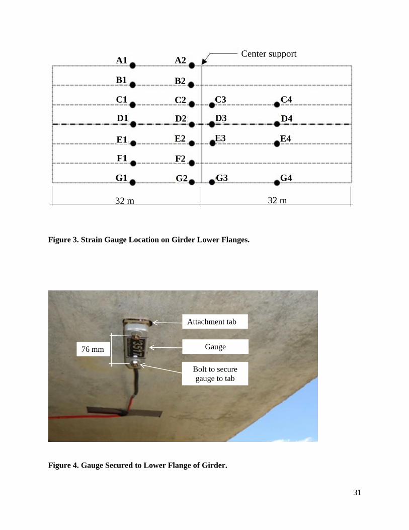
Prior to testing, strain gauges were attached to the lower flange of each girder at the midspans of
the centermost spans, as well as close to the center support (approximately 2 m (6.5 ft) from the
support centerline), as shown in Figure 3. Because only 22 gauges were available, three of the 7
girders were instrumented on one span only, as shown in the figure. The gauge circuit is
composed of a full wheatstone bridge with four active 350 ohm foil gauges, with a power rating
of 13mW at 5V. Excitation voltage is from 1-10 Vdc, with a calibrated strain range of +/- 2000
με. To mount the gauges, two metal tabs on either end of the gauge were secured to the girder
flanges with epoxy after the attachment surface was ground smooth (Figure 4). A careful visual
inspection revealed no cracks on the girder flanges prior to gauge mounting nor during the field
tests. However, it should be noted that some small cracks are elusive and may not have been
seen. Although strain gauges were individually calibrated by the system manufacturer (BDI
2012), the accuracy of all gauges was verified in the laboratory by mounting each gauge to a
steel coupon placed in an MTS tension machine and comparing gauge strains to those found
from displacement results measured from an extensometer in the linear elastic range. Gauges
were found to have an accuracy within 1%, with a noise level in the data acquisition system (BDI
2010) measured at approximately ±1 με. However, strains as low as 1 με could be detected by
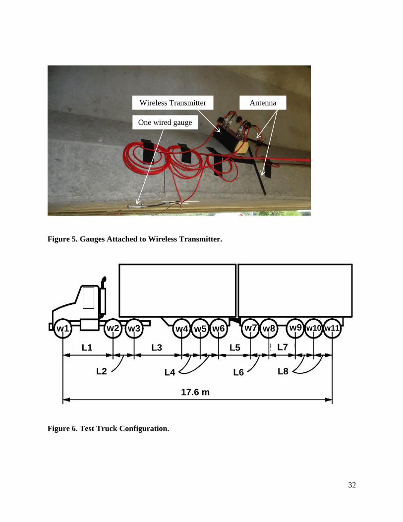
shifts in the noise baseline. Groups of four gauges each were plugged into a wireless transmitter
which was secured on the girder flange, as shown in Figure 5. These transmitters communicated
with a base station, which in turn wirelessly linked to a laptop on-site for data acquisition. Test
data were recorded at a rate of 35 Hz.
Test Plan

7
Two fully-loaded, 11-axle Michigan-legal trucks of 655-685 kN (147-154 kips) gross vehicle
weight each were used to provide live load. This general vehicle configuration is common in
Michigan for heavy legal as well as for permit overloads. Moreover, it is further desirable to use
these heavy truck weights to maximize gauge signal-to-noise ratio as well as to verify load
distribution performance near the upper service load limit. Truck axle weights and spacing were
recorded at a weigh station prior to each test (Tables 1 and 2; Figure 6). Transversely, the front
wheels (single tire) of the vehicles were spaced approximately 2.17 m (7.17 ft) center to center,
while remaining wheels were spaced approximately 1.84 m (6.08 ft) center to center (to the
middle of each double-tire wheel). The trucks were driven across the bridge at crawling speed in
15 different configurations as shown in Figure 7. When side-by-side vehicles were placed close
together (runs 2-4), adjacent wheels were spaced approximately 1.2 m (4 ft) center to center,
while when a vehicle was driven close to the edge of the bridge (runs 3, 4, 13, 15), the center of
wheel was approximately 0.3 m (1 ft) from the edge of the barrier. During the tests, trucks were
carefully guided to ensure adherence to the positions specified in the test plan, and strain data
were continuously recorded as the trucks moved across the bridge. While trucks moved across
the bridges, other traffic was stopped such that no other vehicles were present on the spans.
Test Results
An example diagram showing positive moment (midspan) girder strains as a function of time as
the test vehicles moved across the bridge is shown in Figure 8 (for run 1, bridge 2). Figures 9-11
provide girder strains at midspan (positions A1-G1 and C4-G4 on Figure 3 for span 1 and 2,
respectively) and near the center support (positions A2-G2 and C3-G3 for span 1 and 2,
respectively) for various test runs for the two bridges. The strain profiles shown correspond to
the times at which the truck position produced maximum strains on the girders. In each figure,

8
strains corresponding to the midspan region (positive moment) are shown in the top two
diagrams (a and b), while those corresponding to the center support (negative moment) are
shown in the bottom two diagrams (c and d). In the figures, results are provided for each bridge,
span, and test run. For example, “B1S1-R1” refers to results for (B)ridge 1, (S)pan 1, and (R)un
1.
Figure 9 shows results for runs in which trucks were symmetrically placed in the transverse
direction on the bridge (runs 1, 2, 5, 8, 11). Considering the positive moment results for Bridge
1, the result most apparent, and expected, is that runs 1 and 2 (two trucks side by side) produced
strains approximately twice as high as runs 5, 8, and 11 (trucks in a single lane). It can also be
seen that overall, little difference was found between a single truck (run 11) and multiple trucks
in the same lane (runs 5, 8). However, this is not unexpected, as a single truck length is rather
long for the span, at about half of the span length. Still considering the positive moment results
of span 1 for runs 1 and 2 on Bridge 1, which produced similar results (Figure 9a), it can be seen
that girders to either side (C and E) of the middle girder of the bridge (D) were slightly more
highly loaded. Span 2 results are similar, but in this case the center girder was more heavily
loaded, and the girders overall displayed less uniform load sharing than on span 1. Runs 5 and
11 produced close results on both spans of Bridge 1, while run 8 gave relatively higher strains on
the center three girders. Considering the positive moment results on Bridge 2 (Figure 9b),
overall, similar observations can be made to those of Bridge 1, except loads are less evenly
distributed in general for all runs, with the center girders more highly strained and exterior
girders carrying relatively less load.

9
With regard to negative moment results, it can be seen that negative (i.e. compressive) strains
near the support of Bridge 1 (Figure 9c) are small relative to positive (tension) strains at midspan
(Figure 9a), and as such, may be less reliable measurements of bridge performance. This is not
because of strain gauge sensitivity limitations (see above), but likely the influence of various
other factors, such as unintended differences in support constraint, span continuity, and small
variations in deck or girder stiffness. In particular, for nearly all Bridge 1 runs shown in Figure
9, in which trucks are symmetrically placed on the bridge, the rightmost girder (G) is most
heavily loaded, while strains in the leftmost girder (A) approach zero. However, Bridge 2
negative strain results (Figure 9d), although similar in magnitude to those of Bridge 1, show a
completely different pattern. Here, strains are somewhat more symmetric, and peak in the center
girder, as expected, but also on the outermost girders. Such results appear to indicate that small
variations in joint stiffness from one girder to the next exist at the center support, as suggested
above. Note in particular the slightly positive strains in Figure 9d corresponding to girders A
(0.28 με) and B (1.6 με). Because these small positive strain levels approach the inherent noise
level in the data acquisition system, and are not repeated by any other runs on either structure,
they are regarded as suspect, where the true response is expected to be very slightly negative.
In Figure 10, results are shown for runs in which trucks were placed on the left (A-girder) side of
the bridge (runs 3, 6, 9, 12, 13). For positive moments on Bridge 1 (Figure 10a), as expected,
run 3 (two trucks side by side, close to edge) produced highest girder strains and in the pattern
expected (i.e. strains steadily decreasing away from the girders closest to the vehicles), with run
13 (single truck close to edge) similar but producing lower strains. Run 13 is particularly
interesting in that, in the exterior girder (G) opposite to the side of the bridge that the truck was

10
placed, negative strains were developed at midspan. This was consistent for both spans and both
bridges (Figures 10a and 10b), indicating that extreme eccentric vehicle placement on the bridge
actually caused the deck to deflect the girder upwards on the opposite side of the bridge.
However, when truck eccentricity was decreased from placement at the far edge of the deck
(runs 3, 13) to the center of one lane (runs 6, 9, 12), significant decreases in strains, as well as no
negative strains, resulted (Figures 10a and 10b). Results of Bridge 2 were similar overall to
those of Bridge 1, except that for most runs (all except run 13), strains in exterior girder (A)
decreased somewhat relative to the other girders. Considering the negative moment results for
Bridge 1 (Figure 10c), with the exception of run 3, strains were very low and somewhat uniform.
For run 3, the results were as expected, with the exterior girder closest to trucks (A) being most
heavily loaded while the opposite side exterior girder (G) being most lightly loaded. Bridge 2
negative moment results were closer to that expected for all runs, where a clear trend of
decreasing girder strains away from the girder beneath the truck can be observed. Moreover,
maximum negative girder strains were more than twice as high as those in Bridge 1, which
suggests a greater moment continuity between spans.
In Figure 11, results are provided for runs in which trucks were placed on the right (G-girder)
side of the bridge (runs 4, 7, 10, 14, 15). In Figures 11a and 11b, it can be seen that Bridge 1 and
2 positive moment results are similar, and both mirrored Bridge 2 results in Figure 10b.
Similarly, negative moment results for Bridges 1 and 2 (Figures 11c and 11d) were similar to
those of Bridge 2 in Figure 10d, although negative strains were significantly higher on Bridge 2
than Bridge 1.

11
Numerical Model
To verify the unexpected displacement behavior found in run 13 noted above, where the exterior
girder on the opposite side of the bridge that the truck was placed developed negative strains at
midspan, a simple FEA model of the bridge was constructed. This was a linear elastic model of
approximately 10,000 4-node shell elements to represent equivalent deck, girders, diaphragms,
and barrier stiffnesses, as shown in Figure 12. Support conditions were modeled by constraining
nodes at the underside of the girders in the vertical direction at the end spans and in the vertical
and horizontal direction at the continuous center support; the two end bearings at the continuous
joint, which are relatively close together (center to center spacing 380 mm (15 in)) were modeled
as a single central support. The diaphragms and barriers were modeled with complete
connection to the bridge, where no slip was assumed. Based on field measurements, diaphragm
thickness was taken as 300 mm (12 in). Barrier and girder thickness were taken as 254 mm (10
in) and 429 mm (16.9 in), respectively, which were sized to provide equivalent cross-sectional
area and moment of inertia of the actual components. The heights of components were kept the
same as measured. Young’s modulus for concrete was taken as 31,000 MPa (4500 ksi).
However, the longitudinal Young’s modulus of the elements joining the girders over the center
continuous support was reduced to best-represent the actual degree of center joint continuity, as
discussed in further detail below in the Joint Continuity section of this paper. This simple model
was not meant to represent the bridge in detail, but to verify that the general deformation
behavior as suggested by the measured girder strains for run 13 was reasonable. Results are
shown in Figure 13a, where the model results confirm the compressive (negative) strains
measured during run 13 for the girder on the opposite side of the deck that the truck is placed
(girder G).

12
Girder Distribution Factors
Based on the test results, girder distribution factors (GDFs) were estimated. In this study, GDF
is defined as the maximum proportion of total truck live load effect applied on the bridge that is
distributed to a single girder. Thus GDF, in terms of moment, can be computed as:
n
i i
i
M
MGDF
1
)max( (1)
where Mi is the live load moment carried by girder i and n is the total number of girders.
Expressing moment in terms of Young's modulus (E) and bottom section modulus (S) of girder i
(Mi = EiεiSi), assuming E and S are similar for all girders, GDF can be determined in terms of a
proportion of measured girder strains at the bottom surface of the girder section (ε). It should be
noted that a potential source of inaccuracy with this procedure is that the effective section
modulus and Young’s modulus of the girders are not necessarily constant, due to local variations
in material properties, as well as the presence of non-structural elements on the deck such as
barriers, which stiffen exterior girders to a greater extent than those interior to the span.
Concrete cracking may also represent a source of inaccuracy in this procedure, where although
cracking of the prestressed concrete girders is not expected, cracking of the non-prestressed
continuous joint may be more likely to occur. However, the actual variation in effective girder
stiffness is unknown and can only be approximated. Stallings and Yoo (1993) studied this issue
and estimated the potential effects of edge-stiffening elements on GDF calculation by weighting
exterior girders more heavily in eq. 1. than interior girders. The weighting was conducted by

13
simply including the edge-stiffening curbs in the calculation of exterior girder section modulus.
For composite girders, it was found that this resulted in relatively minor differences in the
resulting GDFs. Nowak and Eom (2001) similarly suggested that only minor differences occur
in GDF when adjusting for edge-stiffening elements. Therefore, given these unknowns and the
relatively small effect that may result from them, possible effective girder stiffness changes are
not considered in eq. 1 and all girders are weighted equally.
The results are presented in Table 3, along with the run (1-15) and girder (A-G) that provided the
maximum GDF reported. Also presented are the GDF values based on the distribution factors
(DF) specified in the AASHTO LRFD Specifications (AASHTO 2012). In AASHTO LRFD, for
interior, prestressed concrete girders supporting a concrete deck with two lanes loaded, the
distribution factor for moment is determined with the empirical expression:
1.0
3
2.06.0
2900075.0
s
g
Lt
K
L
SSDF (2)
where S is girder spacing (mm), L is bridge span (mm), t is deck thickness (mm), and Kg is the
longitudinal stiffness parameter (mm4), a function of the composite girder moment of inertia. A
similar expression with different constants is specified when a single design lane is considered.
For exterior girders, AASHTO specifies that the lever rule is used for one design lane. That is,
the deck is assumed to act as beam spanning transversely from a simple support at the first
interior girder and cantilevered over the adjacent edge (exterior) girder. Design truck wheel
loads are then placed on the beam and the resulting reaction on the exterior girder, as a

14
proportion of the total load, is used to compute DF. When two lanes are considered for exterior
girders, the minimum of the lever rule or a code-specified fractional reduction of the interior
girder DF expression (eq. 2) is used.
For consistent comparison to the experimental GDF values, in Table 3, the 1-lane AASHTO DF
value is divided by 1.2 to remove the included multiple presence factor (other than for the 1-lane
exterior girder case, in which the lever rule governs), while the 2-lane AASHTO value is divided
by 2.0 to account for the fact that the AASHTO DF value is meant to be applied to the weight of
a single design truck rather than to the weight of two trucks as used in the 2-lane field tests.
As shown in Table 3, the positive moment results for both bridges are relatively consistent, with
the largest discrepancy occurring in the 2-lane exterior GDF (0.26 and 0.22 for bridges 1 and 2,
respectively). However, negative moment results between the two structures are much less
consistent, where the closest values obtained were for the 2-lane exterior GDF (0.53 and 0.55),
and the largest proportional discrepancy occurs in the 2-lane interior GDF (0.21 and 0.31). It can
also be seen that, for the 1-lane results, the positive moment GDF for interior girders is
substantially lower than that for exterior girders, but exterior and interior GDFs are about the
same for the 2-lane cases. For the negative moment cases, both interior and exterior GDFs have
large differences for both 1 and 2 lanes, with exterior GDFs about twice the interior values on
average.
As expected, for positive moment, AASHTO results were conservative for both interior and
exterior girders. For negative moments, considering interior girders, AAHSTO was conservative

15
for all cases except for bridge 2, two trucks, run 8 (test 0.31; AASHTO 0.28). However, for
negative moments on exterior girders, 3 of 4 results exceeded AASHTO values, with 2-lane
results significantly so (0.53-0.55 test vs 0.32 AASHTO), where maximums were experienced on
both bridges for run 4. As shown in Figure 7, this run entailed two trucks placed side-by-side
with both vehicles close to an exterior girder. This latter result is an unexpected finding, as it
was anticipated that the governing method specified by AASHTO (2012) for exterior girder DF
(per sections 4.6.2.2.2d and C4.6.2.2.2d), would result in the maximum possible load effect to
the girder. However, the field test results of both bridges suggest that, for this particular type of
structure, this method (as well as the lever rule) may significantly under-predict the DF for
exterior girders when negative moments are considered.
If used to predict future performance, one way that the confidence of GDF results can be judged
is by examining the degree of consistency from one structure to the next. For example, consider
the exterior girder cases for negative moment. For the side-by-side trucks case, results from both
structures are relatively consistent, as shown in Table 3 (GDFs of 0.53 and 0.55), and are also
governed by the same run and girder on both structures (4G). Thus for this particular case, it
appears reasonable to conclude that the AASHTO result (0.32) is indeed significantly
unconservative for the field test structures. In contrast, for the single lane case, a fairly large
discrepancy between bridges exists (GDFs of 0.48 and 0.56). However, the AASTHO prediction
(0.51) also falls within this range, indicating that the AASHTO value appears reasonable. That
said, the wider discrepancy in test results for the single lane case suggests that its GDF is known
with less certainty than that of the side-by-side trucks case.

16
To confirm this finding, the FEA model discussed above was used to simulate various runs,
some examples of which are shown in Figure 11. In addition to the run 13 result discussed
earlier (Figure 13a), an example result showing the positive moment strains for run 1 (Figure
13b) is provided, representing typical model accuracy. The negative moment results of concern,
those for run 4, are presented in Figure 13c. In general, it was found that FEA results well-
matched the field tests, suggesting that the model can be used with reasonable confidence. As
seen in Figure 13c, the model indeed verifies the field test results of concern, producing
approximately the same very high negative moment GDF for run 4. It should also be noted that
when the joint was taken as fully continuous in the FEA model, the negative moment GDFs
decreased significantly such that the AASHTO values shown in Table 3 were found to be
conservative, as expected. For example, for the side-by-side trucks case, when run 4 was
considered, the negative moment GDF dropped from 0.53 for the partial continuity case (as
found from the field test of bridge 1 as well as the FEA model) to 0.26 for the fully continuous
case, below the AASHTO value of 0.32.
Joint Continuity
For each test run, strains along the length of the bridge girders were evaluated when the trucks
were in various positions. Of particular interest was the variation of strain along the length of the
girder when the trucks were placed to generate maximum positive moment. An example of these
results from run 1 is shown in Figure 14, when the truck was located near the middle of the
leftmost span, maximizing strains at girder line 1 (i.e. at gauges A1-G1 as shown in Figure 3).
These results are reported in Figure 14 as the “Bridge 1” and “Bridge 2” results (taken as the
average of the middle three girders, C, D, and E). Although maximum strains differ,

17
proportional results from other tests runs are nearly identical to those shown in Figure 14 and are
thus not shown.
Also shown in Figure 14 is the result of the FEA model. As noted above, the longitudinal (in-
plane, in the direction of the span of the girders) modulus of elasticity of a vertical line of shell
elements through the depth of each girder, located directly over the continuous center support,
Exj, was adjusted until the longitudinal distribution of strains measured at the gauge positions 1-4
(taken as the average of the three central girders) best-matched those of the field test results.
This reduction in modulus was chosen to represent the effective rotational stiffness of the actual
continuous bridge joint as accurately as possible. Here, it was found that reducing Exj from the
initial value of 31000 MPa (4500 ksi) to only 900 MPa (130 ksi) allowed the model to produce
nearly identical results as found in the field test, as shown in Figure 14. It was this model that
was used earlier to successfully match the transverse distribution of strains, as shown in Figure
13.
As the concern for evaluating joint continuity is the longitudinal distribution of load along the
bridge rather than transversely, the possibility of constructing a much simpler model was
investigated. In this alternative approach, each span of the bridge was modeled as a single
prismatic beam. The beam spans were roller-supported at end supports and connected with a
rotational spring over the center support, for which the vertical and horizontal translations were
restrained only. Similar to the process used to calibrate the joint stiffness of the FEA model, the
stiffness of the rotational spring joining the spans at the center support of the beam model was
adjusted, such that the proportion of moments along the span best-matched the proportion of

18
girder strains in the field tests at the same locations. An effective conversion factor transforming
model moments to ‘actual’ expected strains in a bridge girder can then be developed by diving
the strain found in the field test by the analysis model moment corresponding to the same section
(the average value found at each location 1-4 is used as a constant conversion factor for all 4
strain locations to produce an analytically consistent model). These results are shown in Figure
14 as the ‘Calibrated beam model’ results. As shown in the figure, excellent agreement was
obtained between the proportional distribution (along the length of the bridge) of model to field
test strains, indicating that this very simple model can just as effectively represent the actual
longitudinal distribution of moments along the span of the bridge as can the much more complex
FEA model. For further verification, the model results were compared to the field test results
when trucks were placed on the opposite span position (i.e. truck placed at position 4, rather than
at position 1, as shown at the bottom of Figure 14), and no significant difference in accuracy was
found. Further, although run 1 results were initially used to develop the model, similarly good
agreement was obtained using the model and comparing proportions of model moments and field
test strains from three additional runs as well (9, 11, and 12). Results were nearly identical in
each case.
To quantify the effective rotational stiffness of the center joint of the bridges, the model was
reanalyzed with completely simple (i.e. joint rotational stiffness = 0; two independent spans) and
completely continuous (joint rotational stiffness = infinite) cases. The moment–strain conversion
factor determined above was then used to similarly convert the simple and continuous case
moments into equivalent strains, which are also shown in Figure 14. As shown in the figure, as

19
expected, the actual structure appears to fall between a simple and continuous span, with results
closer to a simple span.
Additional results are shown in Table 4 for four additional runs that were modeled (1, 9, 11, 12).
In the table, “continuous/actual” refers to the ratio of a continuous span strain compared to the
actual strain; “simple/actual” refers to the ratio of a simple span strain compared to the actual
strain; and “near” refers to the span on which the truck is placed, while “far” refers to the
opposite span. Although table results are shown for the truck positioned on the leftmost span as
the near span (position 1 in Figure 14), placing the truck on span 2 (position 4 in Figure 14)
produced nearly identical results, as noted above. As shown in Table 4, little variation was
found in results from one run to another.
Based on the results of Table 4, the maximum positive moment is 1/0.84 or about 20% higher
than that found from a completely continuous support, while negative moments (as well as far
span positive moments) are approximately 1/3.62, or less than 30% of that found from a
completely continuous support. When compared to a simple span, the average ratio of the
maximum positive simple span moment to actual (model) moments was found to be about 1.07,
as shown in the table. In summary, the results indicate that a simple span would produce a
maximum positive moment about 7% higher than the actual structure, while a completely
continuous structure would produce a maximum positive moment about 16% lower than the
actual structure.
20
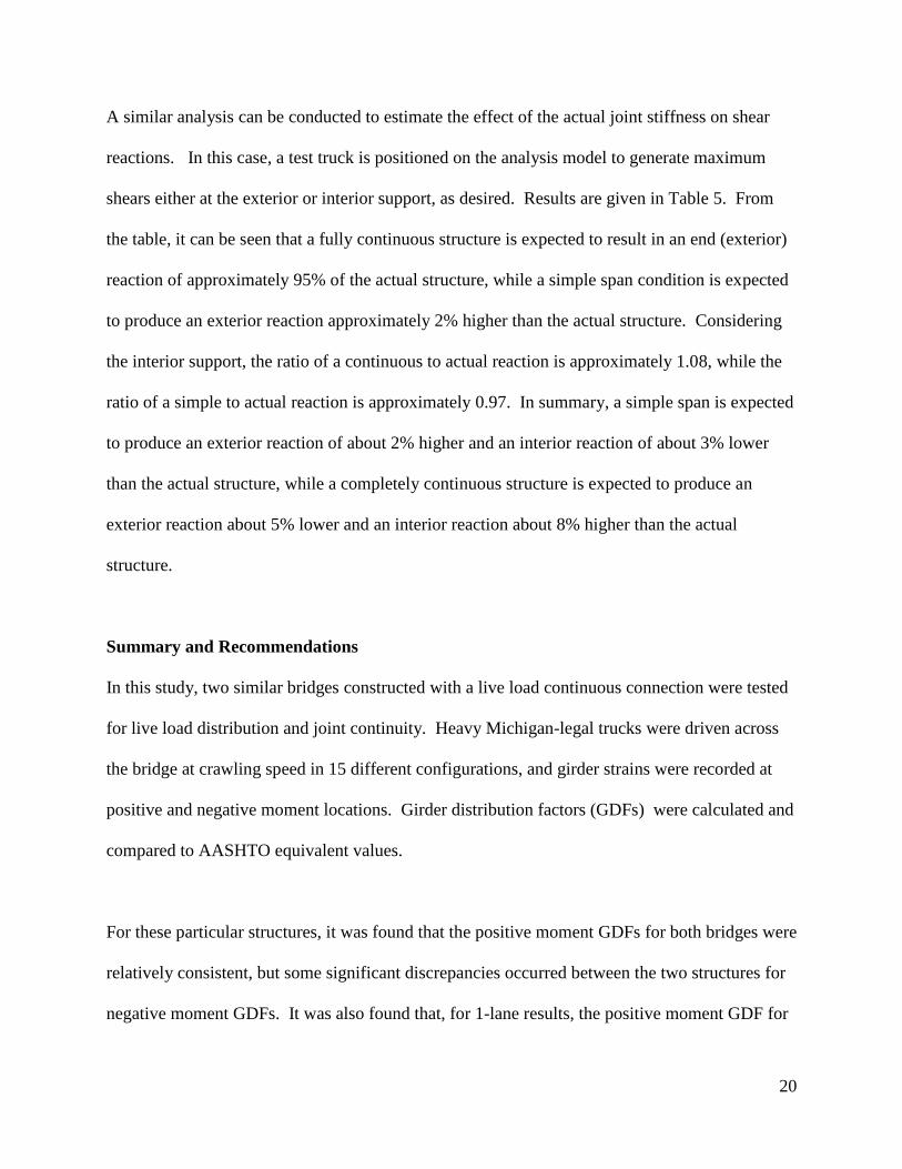
A similar analysis can be conducted to estimate the effect of the actual joint stiffness on shear
reactions. In this case, a test truck is positioned on the analysis model to generate maximum
shears either at the exterior or interior support, as desired. Results are given in Table 5. From
the table, it can be seen that a fully continuous structure is expected to result in an end (exterior)
reaction of approximately 95% of the actual structure, while a simple span condition is expected
to produce an exterior reaction approximately 2% higher than the actual structure. Considering
the interior support, the ratio of a continuous to actual reaction is approximately 1.08, while the
ratio of a simple to actual reaction is approximately 0.97. In summary, a simple span is expected
to produce an exterior reaction of about 2% higher and an interior reaction of about 3% lower
than the actual structure, while a completely continuous structure is expected to produce an
exterior reaction about 5% lower and an interior reaction about 8% higher than the actual
structure.
Summary and Recommendations
In this study, two similar bridges constructed with a live load continuous connection were tested
for live load distribution and joint continuity. Heavy Michigan-legal trucks were driven across
the bridge at crawling speed in 15 different configurations, and girder strains were recorded at
positive and negative moment locations. Girder distribution factors (GDFs) were calculated and
compared to AASHTO equivalent values.
For these particular structures, it was found that the positive moment GDFs for both bridges were
relatively consistent, but some significant discrepancies occurred between the two structures for
negative moment GDFs. It was also found that, for 1-lane results, the positive moment GDF for

21
interior girders was substantially lower than that for exterior girders, but exterior and interior
GDFs were about the same for the 2-lane cases. For the negative moment cases, however,
exterior GDFs were about twice the interior values on average.
For positive moments on all girders as for negative moments on interior girders, AASHTO
results were generally conservative. However, for negative moments on exterior girders, 3 of 4
cases exceeded AASHTO values, with 2-lane results significantly so. GDF results were verified
with a FEA model, which produced similar behavior to the field tests.
With respect to joint continuity, it was found that a FEA model, as well as a simple prismatic
beam model, could well-replicate the test results. Based on calibrated model results, it is
estimated that a simple span would produce a maximum positive moment about 7% higher than
the actual structure, while a completely continuous structure would produce a maximum positive
moment about 16% lower than the actual structure. For negative moments, the actual structure
experienced about 28% of that of a continuous structure. Similarly, for shear, it is estimated that
a simple span would produce an exterior reaction of about 2% higher and an interior reaction of
about 3% lower than the actual structure, while a completely continuous structure would produce
an exterior reaction about 5% lower and an interior reaction about 8% higher than the actual
structure.
Based on these results, some recommendations for these particular types of structures can be
made as follows. For GDF, as expected, for both positive and negative moment, AASHTO
recommendations for interior and exterior girders when a single lane is considered, as well as for

22
interior girders when two lanes are considered, are generally conservative, or reasonably close to,
field test results. For these cases, the existing AASHTO procedures appear reasonable.
However, for the particular case of two lanes loaded when negative moments on exterior girders
are considered, the procedure suggested by AASHTO was shown to significantly underestimate
GDF on both structures. In this case, a more refined analysis than that provided by AASHTO is
strongly recommended.
To model the effect of the live load continuous joint, a conservative approach would be to simply
assume that the structure is continuous for negative live load moments and simply spanning for
positive live load moments. Similarly, for shear, the structure can conservatively be assumed
continuous for interior reactions and simple for exterior reactions. However, for a more precise
estimation of load effect, based on the field test and modeling results, for positive and negative
moments as well as shears at interior and exterior supports, good agreement to the test results in
all of these cases can be obtained with the following expression:
Q = 0.3Qc + 0.7Qs (3)
In this expression, Q is the final load effect (either moment or shear), and Qc is the load effect
found from analysis of a completely continuous structure, while Qs is the load effect found from
analysis of a simple spanning structure (for negative moments, note Qs = 0). The factors 0.3 and
0.7 result from the fact that in all cases considered, the actual load effect is approximately twice
as close to that of a simple structure as compared to a continuous structure. For other live-load
continuous joints, the factors 0.3 and 0.7 can be adjusted appropriately based on field test results.

23
Some additional issues should be noted. First, it should be emphasized that these results are
based on the particular structures investigated and are not necessarily applicable to other live
load continuous joint designs. Second, although heavy loads were used in the field tests, these
remain service loads and the structure behaved linear-elastically. At higher load levels closer to
an actual failure condition, it is possible that joint stiffness may further decrease to more closely
resemble that of a simple connection. Unfortunately, there is no simple way to determine joint
stiffness for all live-load continuous bridges, as this will depend significantly on various factors
including construction technique and level of deterioration. To estimate the degree of joint
continuity, a process similar to that described in this study is recommended, where girders are
instrumented and several test runs with known vehicle configurations are conducted to record
strains. For new construction, in lieu of specific field testing, it may be ideal to mount
permanent strain gauges on reinforcing bars within the bridge members as well as on the
concrete surface for continuous monitoring of the continuous joint as well as girder behavior. In
either case, a simple, prismatic beam model of the bridge can be quickly constructed, with a
rotational spring connecting the spans, as described above. The rotational spring can be altered
until proportions of positive and negative moments in the model well-match the proportion of
strains at the same locations on the actual structure. Such a match suggests that the simple model
can be reasonably used to represent the joint stiffness of the actual structure. Finally, when
considering negative moment for exterior girders, although GDFs were found to be significantly
higher than AASHTO values, the overall girder design remains rather conservative. This is
because the actual live load negative moment is only about 30% of that caused by the fully

24
continuous joint as assumed in design. This reduction in moment more than offsets the under-
prediction of GDF.

25
References
AASHTO (2012). AASHTO LRFD Bridge Design Specifications, 6th Ed., Washington, DC.
Bakht, B. and Csagoly, P.F. (1980). “Diagnostic testing of a bridge.” Journal of the Structural
Division 106(7), 1515-1529.
Bakht, B., and Jaeger, L.G. (1990). “Bridge testing. A surprise every time.” Journal of Structural
Engineering New York 116(5), 1370-1383.
Barr, P.J., Eberhard, M.O., and Stanton, J.F. (2001). “Live-load distribution factors in prestressed
concrete girder bridges.” Journal of Bridge Engineering 6(5), 298-306.
Bridge Diagnostics, Inc. (2010). “Wireless Structural Testing System STS-WiFi Operations
Manual” BDI, Boulder, CO.
Bridge Diagnostics, Inc. (2012). “ST350 Operations Manual” BDI, Boulder, CO.
Cai, C.S. (2005). “Discussion on AASHTO LRFD load distribution factors for slab-on-girder
bridges.” Practice Periodical on Structural Design and Construction 10:3, 171-176.
Cai, C.S. and Shahawy, M. (2004). “Predicted and measured performance of prestressed concrete
bridges.” Journal of Bridge Engineering 9:1, 4-13.
Cross et al. (2009). “Analytical and experimental investigation of bridge girder shear distribution
factors.” Journal of Bridge Engineering 14(3), 154-163.
Darlow, M.S. and Bettigole, N.H. (1989). “Instrumentation and testing of bridge rehabilitated
with exodermic deck.” Journal of Structural Engineering New York 115(10), 2461-2480.
Dicleli, M. and Erhan, S. (2009). “Live load distribution formulas for single-span prestressed
concrete integral abutment bridge girders.” Journal of Bridge Engineering 14(6), 472-
486.

26
Eamon, C., and Nowak, A.S. (2002). “Effects of edge-stiffening elements and diaphragms on
bridge resistance and load distribution.” Journal of Bridge Engineering 7(5), 258-266.
Eom, J. and Nowak, A.S. (2001). “Live load distribution for steel girder birdges.” Journal of
Bridge Engineering 6:6, 489-497.
Fanous, F., May, J., and Wipf, T. (2011). “Development of live-load distribution factors for
glued-laminated timber girder bridges.” Journal of Bridge Engineering 16:2, 179-187.
Ghosn, M., Moses, F., and Gobieski, J. (1986). “Evaluation of steel bridges using in-service
testing.” Transportation Research Record 1072, Transportation Research Board,
Washington, DC. 71-78.
Harris, D.K. (2010). “Assessment of flexural lateral load distribution methodologies for stringer
bridges.” Engineering Structures 32:11, 3443-3451.
Hughs, E. (2006). “Live-load distribution factors for prestressed concrete, spread box-girder
bridge.” Journal of Bridge Engineering 11(5), 573-581.
Li, M., Hashimoto, K., and Sugiura, K. (2014). “Influence of Asphalt Surfacing on Fatigue
Evaluation of Rib-to-Deck Joints in Orthotropic Steel Bridge Decks.” Journal of Bridge
Engineering 19(10).
Miller, R.A., Castrodale, R., Mirmiran, A., and Hastak, M. (2004). “Connection of simple-span
precast concrete girders for continuity.” NCHRP Report 519. Transportation Research
Board, Washington, D.C.
Nowak, A.S. and Eom, J. (2001). “Verification of girder distribution factors for steel girder
bridges.” MDOT Research Report RC-1393. Michigan Department of Transportation,
Lansing, MI.

27
Ebeido, Tarek, and John B. Kennedy. (1996). "Girder moments in continuous skew composite
bridges." Journal of Bridge Engineering 1(1), 37-45.
Oesterle, R., Mehrabi, A.B., Tabatabai, H., Scanlon, A., and Ligozio, C.A. (2004). “Continuity
considerations in prestressed concrete jointless bridges.” Proceedings, 2004 Structures
Congress, 227-234.
Okeil, A. and Elsafty, A. (2005). “Partial continuity in bridge girders with jointless decks.”
Practice Periodical on Structural Design and Construction 10(4), 229-238.
Puckett, J.A., Sharon, X.H., Jabllin, M., and Mertz, D.R. (2012). “Framework for Simplified
Live Load Distribution-Factor Computations.” Journal of Bridge Engineering 16:6, 777-
791.
Seo, J., Phares, B., Wipf, T.J. (2014). “Lateral Live-Load Distribution Characteristics of Simply
Supported Steel Girder Bridges Loaded with Implements of Husbandry.” Journal of
Bridge Engineering 19:4, 1943-5592.
Shepherd, R. and Sidwell, G.K. (1973). “Composite Road Bridges.” Highways and Road
Construction 41(1767), 20-25.
Stallings, J.M., and Yoo, C.H. (1993). “Tests and ratings of short span bridges.” Journal of
Structural Engineering 19:7, 2150-2168.
Yousif, Z. and Hindi, R. (2007). “AASHTO-LRFD live load distribution for beam-and-slab
bridges: Limitations and applicability.” Journal of Bridge Engineering 12:6, 765-773.
Zia, P., Caner, A., and El-Safty, A.K. (1995). “Jointless bridge decks.” Final Report, North
Carolina Department of Transportation.
Zokaie, T. and Imbsen, R.A. (1992). “Distribution of wheel loads on highway bridges.” NCHRP
12-26. National Cooperative Highway Research Program, Washington, DC.

28
Table 1. Axle Weights of Test Vehicles.
Truck Axle weights, kN (kips)
w1 w2 w3 w4 w5 w6 w7 w8 w9 w10 w11
Bridge 1
truck 1 57.9
(13.0)
58.7
(13.2)
75.2
(16.9)
46.7
(10.5)
82.3
(18.5)
49.0
(11.0)
52.5
(11.8)
66.3
(14.9)
54.3
(12.2)
62.3
(14.0)
67.2
(15.1)
truck 2 69.9
(15.7)
59.2
(13.3)
77.0
(17.3)
49.8
(11.2)
51.6
(11.6)
77.9
(17.5)
48.5
(10.9)
60.1
(13.5)
48.5
(10.9)
55.2
(12.4)
55.2
(12.4)
Bridge 2
truck 1 63.2
(14.2)
61.9
(13.9)
77.0
(17.3)
48.1
(10.8)
53.4
(12.0)
66.3
(14.9)
60.5
(13.6)
69.9
(15.7)
53.0
(11.9)
57.9
(13.0)
64.5
(14.5)
truck 2 69.9
(15.7)
59.6
(13.4)
85.0
(19.1)
43.4
(9.8)
54.3
(12.2)
80.1
(18.0)
51.6
(11.6)
68.5
(15.4)
50.7
(11.4)
57.0
(12.8)
66.3
(14.9)
Table 2. Axle Spacing of Test Vehicles.
Truck Axle Spacing, m (ft)
L1 L2 L3 L4 L5 L6 L7 L8
truck 1 3.71
(12.2)
1.29
(4.3)
3.23
(10.7)
1.11
(3.7)
2.30
(7.6)
1.11
(3.7)
1.52
(5.0)
1.12
(3.7)
truck 2 3.58
(11.8)
1.34
(4.4)
2.88
(9.5)
1.11
(3.7)
2.40
(7.9)
1.11
(3.7)
1.64
(5.4)
1.12
(3.7)
Table 3. Maximum Proportion of Total Live Load Moment on Span Applied to a Single
Girder.
Truck(s) in a Single Lane Trucks Side-by-Side
GDF Type Bridge 1 Bridge 2 AASHTO Bridge 1 Bridge 2 AASHTO*
Interior, +M 0.26 (13B,15F) 0.23 (13B) 0.35 0.24 (4F) 0.24 (5D) 0.28
Interior, -M 0.20 (12C) 0.29 (6C) 0.35 0.21 (3B,4F) 0.31 (8D) 0.28
Exterior, +M 0.35 (15G) 0.36 (13A) 0.51 0.26 (3A) 0.22 (3A,4G) 0.32
Exterior, -M 0.48 (15G) 0.56 (13A) 0.51 0.53 (4G) 0.55 (4G) 0.32 *AASHTO DF for two lanes loaded is reduced by ½ to correspond to GDF as defined in this study (see text).

29
Table 4. Moment Ratios.
Bridge 1 Bridge 2
Location, Run continuous
/ actual
simple
/actual
continuous /
actual
simple
/actual
+M (near), R1 0.84 1.07 0.84 1.06
+M (near), R9 0.83 1.08 0.84 1.08
+M (near), R11 0.84 1.06 0.84 1.06
+M (near), R12 0.84 1.06 0.84 1.06
-M, R1 3.60 - 3.60 -
-M, R9 3.62 - 3.62 -
-M, R11 3.58 - 3.67 -
-M, R12 3.58 - 3.67 -
+M (far), R1 3.60 - 3.60 -
+M (far), R9 3.62 - 3.62 -
+M (far), R11 3.67 - 3.67 -
+M (far), R12 3.67 - 3.67 - Continuous and simple refer to idealized joint conditions in the model while
actual refers to the degree of continuity measured from field test results.
Table 5. Shear Ratios.
Bridge 1 Bridge 2
Location, Run continuous
/ actual
simple
/actual
continuous /
actual
simple
/actual
Exterior, R1 0.95 1.03 0.95 1.02
Exterior, R9 0.91 1.04 0.91 1.03
Exterior, R11 0.95 1.02 0.95 1.02
Exterior, R12 0.95 1.02 0.95 1.02
Interior, R1 1.08 0.97 1.07 0.97
Interior, R9 1.09 0.97 1.10 0.97
Interior, R11 1.07 0.98 1.08 0.97
Interior, R12 1.07 0.98 1.08 0.97 Continuous and simple refer to idealized joint conditions in the model while
actual refers to the degree of continuity measured from field test results.

30
Figure 1. MDOT Live-load Continuous Connection.
Figure 2. Bridge Cross-Section.
Type IV
7 girders spaced at 1.9 m
12 m 0.45 m 0.45 m
230 mm slab
A B C D E F G
Continuous slab over pier
Girder Type IV Girder Type IV
Diaphragm
31
Figure 3. Strain Gauge Location on Girder Lower Flanges.
Figure 4. Gauge Secured to Lower Flange of Girder.
Center support A1
B1
C1
D1
E1
F1
G1
A2
B2
C2
D2
E2
F2
G2
C3
D3
E3
G3
C4
D4
E4
G4
32 m 32 m
Gauge
Attachment tab
Bolt to secure
gauge to tab
76 mm
32
Figure 5. Gauges Attached to Wireless Transmitter.
Figure 6. Test Truck Configuration.
Wireless Transmitter
One wired gauge
Antenna
L1
L2
L3
L4
L5
L6
L7
L8
17.6 m
w1 w2 w3 w4 w5 w6 w7 w8 w9 w10 w11

33
Figure 7. Vehicle Test Plan.

34
Figure 8. Midspan Girder Strains for Run 1, Bridge 2.
Girder
-20
0
20
40
60
80
100
120
A B C D E F G
Mic
rost
rain
B1S1-R1
B1S1-R2
B1S1-R5
B1S1-R8
B1S1-R11
B1S2-R1
B1S2-R2
B1S2-R5
B1S2-R8
B1S2-R11
Girder
-20
0
20
40
60
80
100
120
A B C D E F G
Mic
rost
rain
B2S1-R1
B2S1-R2
B2S1-R5
B2S1-R8
B2S1-R11
B2S2-R1
B2S2-R2
B2S2-R5
B2S2-R8
B2S2-R11
Girder
-20
-15
-10
-5
0
5
A B C D E F G
Mic
rost
rain
B1S1-R1
B1S1-R2
B1S1-R5
B1S1-R8
B1S1-R11
B1S2-R1
B1S2-R2
B1S2-R5
B1S2-R8
B1S2-R11Girder
-20
-15
-10
-5
0
5
A B C D E F G
Mic
rost
rain
B2S1-R1
B2S1-R2
B2S1-R5
B2S1-R8
B2S1-R11
B2S2-R1
B2S2-R2
B2S2-R5
B2S2-R8
B2S2-R11
Figure 9. Girder Strains for Trucks Centered on Bridge (Runs 1, 2, 5, 8, 11).
Girder
D
E
C
B
F
A
G
(a) Positive Moments, Bridge 1 (b) Positive Moments, Bridge 2
(c) Negative Moments, Bridge 1 (d) Negative Moments, Bridge 2

35
Girder
-20
0
20
40
60
80
100
120
A B C D E F G
Mic
rost
rain
B1S1-R3
B1S1-R6
B1S1-R9
B1S1-R12
B1S1-R13
B1S2-R3
B1S2-R6
B1S2-R9
B1S2-R12
B1S2-R13Girder
-20
0
20
40
60
80
100
120
A B C D E F G
Mic
rost
rain
B2S1-R3
B2S1-R6
B2S1-R9
B2S1-R12
B2S1-R13
B2S2-R3
B2S2-R6
B2S2-R9
B2S2-R12
B2S2-R13
Girder
-30
-25
-20
-15
-10
-5
0
5
A B C D E F G
Mic
rost
rain
B1S1-R3
B1S1-R6
B1S1-R9
B1S1-R12
B1S1-R13
B1S2-R3
B1S2-R6
B1S2-R9
B1S2-R12
B1S2-R13Girder
-30
-25
-20
-15
-10
-5
0
5
A B C D E F G
Mic
rost
rain
B2S1-R3
B2S1-R6
B2S1-R9
B2S1-R12
B2S1-R13
B2S2-R3
B2S2-R6
B2S2-R9
B2S2-R12
B2S2-R13
Figure 10. Girder Strains for Trucks on Left Side of Bridge (Runs 3, 6, 9, 12, 13).
Girder
-20
0
20
40
60
80
100
120
A B C D E F G
Mic
rost
rain
B1S1-R4
B1S1-R7
B1S1-R10
B1S1-R14
B1S1-R15
B1S2-R4
B1S2-R7
B1S2-R10
B1S2-R14
B1S2-R15Girder
-20
0
20
40
60
80
100
120
A B C D E F G
Mic
rost
rain
B2S1-R4
B2S1-R7
B2S1-R10
B2S1-R14
B2S1-R15
B2S2-R4
B2S2-R7
B2S2-R10
B2S2-R14
B2S2-R15
Girder
-45
-40
-35
-30
-25
-20
-15
-10
-5
0
5
A B C D E F G
Mic
rost
rain
B1S1-R4
B1S1-R7
B1S1-R10
B1S1-R14
B1S1-R15
B1S2-R4
B1S2-R7
B1S2-R10
B1S2-R14
B1S2-R15Girder
-45
-40
-35
-30
-25
-20
-15
-10
-5
0
5
A B C D E F G
Mic
rost
rain
B2S1-R4
B2S1-R7
B2S1-R10
B2S1-R14
B2S1-R15
B2S2-R4
B2S2-R7
B2S2-R10
B2S2-R14
B2S2-R15
(a) Positive Moments, Bridge 1 (b) Positive Moments, Bridge 2
(c) Negative Moments, Bridge 1 (d) Negative Moments, Bridge 2
(a) Positive Moments, Bridge 1 (b) Positive Moments, Bridge 2
(c) Negative Moments, Bridge 1 (d) Negative Moments, Bridge 2

36
Figure 11. Girder Strains for Trucks on Right Side of Bridge (Runs 4, 7, 10, 14, 15).
Figure 12. FEA Model of Bridge.
-10
0
10
20
30
40
50
60
70
80
90
100
A B C D E F G
Girder
Mic
ro
stra
in
Bridge 1
Bridge 2
Model
0
10
20
30
40
50
60
70
80
90
100
A B C D E F G
Girder
Mic
ro
stra
in
Bridge 1
Bridge 2
Model
-45
-40
-35
-30
-25
-20
-15
-10
-5
0
5
A B C D E F G
Girder
Mic
ro
stra
in
Bridge 1
Bridge 2
Model
Figure 13. Comparison of FEA Model and Field Test Results for Runs 13, 1, and 4.
Underside of one span,
undeformed state.
Bridge in deformed
state, run 13 loading.
(a) Run 13, Positive Moment (b) Run 1, Positive Moment (c) Run 4, Negative Moment

37
Figure 14. Distribution of Strains Along Girders for Run 1.
(1) (2) (3) (4)
Location
2 1 3 4