Field trials of an energy‐aware mission planner

General rights Copyright and moral rights for the publications made accessible in the public portal are retained by the authors and/or other copyright owners and it is a condition of accessing publications that users recognise and abide by the legal requirements associated with these rights.

Users may download and print one copy of any publication from the public portal for the purpose of private study or research.

You may not further distribute the material or use it for any profit-making activity or commercial gain

You may freely distribute the URL identifying the publication in the public portal If you believe that this document breaches copyright please contact us providing details, and we will remove access to the work immediately and investigate your claim.

Downloaded from orbit.dtu.dk on: Oct 19, 2021

Field trials of an energy-aware mission planner implemented on an autonomoussurface vehicle

Thompson, Fletcher; Galeazzi, Roberto; Guihen, Damien

Published in:Journal of Field Robotics

Link to article, DOI:10.1002/rob.21942

Publication date:2020

Document VersionPeer reviewed version

Link back to DTU Orbit

Citation (APA):Thompson, F., Galeazzi, R., & Guihen, D. (2020). Field trials of an energy-aware mission planner implementedon an autonomous surface vehicle. Journal of Field Robotics, 37(6), 1040-1062.https://doi.org/10.1002/rob.21942

https://doi.org/10.1002/rob.21942

https://orbit.dtu.dk/en/publications/e7b26c19-bd67-4729-8552-1b9d145be779


Field Trials of an Energy Aware Mission Planner

Implemented on an Autonomous Surface VehicleFletcher Thompson∗

Section for Oceans and Arctic

Technical University of Denmark

Building 201, Kemitorvet, 2800 Kgs. Lyngby, Denmark

[email protected]

Roberto Galeazzi

Automation and Control

Technical University of Denmark

Building 326, Elektrovej, 2800 Kgs. Lyngby, Denmark

[email protected]

Damien Guihen

National Centre for Maritime Engineering and Hydrodynamics

University of Tasmania

Newnham Drive, Newnham, Tasmania, Australia

[email protected]

AbstractMission planning for Autonomous Marine Vehicles (AMVs) is non-trivial due to the

dynamic and uncertain nature of the marine environment. Communication can be low-∗Corresponding Author

This is the author manuscript accepted for publication and has undergone fullpeer review but has not been through the copyediting, typesetting, paginationand proofreading process, which may lead to differences between this versionand the Version of Record. Please cite this article as doi: 10.1002/rob.21942

Aut

hor M

anus

crip

t

This article is protected by copyright. All rights reserved.

Thompson Fletcher ORCID iD: 0000-0002-0639-9871



http://crossmark.crossref.org/dialog/?doi=10.1002%2Frob.21942&domain=pdf&date_stamp=2020-02-11

bandwidth and is not always guaranteed, so the operator must rely on the vehicles

to adjust their plans according to the realised state of the environment. This paper

presents the improvements made to an energy-aware mission planner that allow it to

generate and adjust plans for an Autonomous Surface Vehicle (ASV) operating in an

uncertain environment. The energy-aware mission planning problem was redefined as

a stochastic programming problem, and a two-stage solver was developed to provide

an initial plan for the ASV and then adjust it during run-time according to pre-defined

recourse actions. The mission planner and ASV were trialled in Lake Waverley, Tas-

mania. Adjusting the recourse action criteria demonstrated that the ASV could ex-

hibit conservative or opportunistic behaviours according to the operator’s preference

of safety margin. In the pursuit of extending the planner’s second-stage so that it can

predict a suitable recourse action ahead of time, a hybrid Long Short-Term Memory

energy forecaster was trained from the Waverley mission data. Comparison of the er-

ror between the forecaster and the test data shows that the forecaster has a reliable

forecast horizon of about 10 seconds.

Aut

hor M

anus

crip

t


List of Acronyms

AMV Autonomous Marine Vehicle

ASV Autonomous Surface Vehicle

AUV Autonomous Underwater Vehicle

DC Direct Current

EKF Extended Kalman Filter

EUROPtus Extensible Universal Remote Operations Planning with Neptus

GPS Global Positioning System

GUI Graphical User Interface

HMI Human-Machine Interface

IMU Inertial Measurement Unit

LOS Line of Sight

LSTM Long Short-Term Memory

OP-SW Orienteering Problem with Stochastic Weights

OR Operations Research

PID Proportional Integral Derivative

PSO Particle Swarm Optimisation

PSR Point of Safe Return

RC Radio Controller

Aut

hor M

anus

crip

t


RMSE Root-Mean-Squared Error

RNN Recurrent Neural Networks

ROS Robot Operating System

SAA Sample Average Approximation

TOP Team Orienteering Problem

T-REX Teleo-Reactive Executive

UTM Universal Transverse Mercator

1 Introduction

This paper considers automated mission energy planning and forecasting for Autonomous Marine

Vehicles (AMVs) with electric power supplies. The energy supply of an AMV is vital to its successful

operation, power failures are one of the leading causes of overall mission failure (Brito et al., 2014).

Effectively managing the energy supply means not only ensuring that the AMV does not overextend

itself with an overambitious mission plan, it also means making the most use of the available energy of

the vehicle to achieve as many mission tasks as possible. Currently, operators balance the survival of

their vehicle and its task completion effectiveness by consulting the manufacturer specifications (e.g.

range, endurance, rated depth) and applying safety factors to those specifications in order to obtain

safe mission planning constraints. In pursuit of refining this balance to maximise the effectiveness

of the vehicle while still maintaining survivability, this paper considers energy management from an

onboard mission planning and decision-making approach.

The reasoning and deliberation capabilities of AMVs have blossomed over the last decade. Prior to

2008, mission planning for AMVs was a task reserved for the human operator, who would create a

Aut

hor M

anus

crip

t


scripted set of way-points, depths, speeds, control modes, and sensor payload modes. This procedure

relied on the operator’s experience to predict the reliability of the mission script, and to adequately

prepare the vehicle with contingencies for outcomes that are likely to occur. McGann et al. (2008)

ushered in a new method of planning for AMVs by implementing the deliberative Teleo-Reactive

Executive (T-REX) agent onboard Autonomous Underwater Vehicles (AUVs). T-REX effectively

allows vehicles to adjust their plan and behaviours during execution according to detected external

changes and inferred changes to the mission state.

With AMVs able to adapt plans in order to achieve mission objectives, automated mission planning

has been extended to dynamically generate and adapt mission plans for large operations. Mesoscale

(≥ 50 km2) coordinated multi-AMV operations have been realised through the development and

implementation of temporal planners such as Extensible Universal Remote Operations Planning with

Neptus (EUROPtus) (Py et al., 2016). Temporal plans schedule and allocate tasks to the vehicles using

time as the base resource constraint. A partial plan is instantiated and is refined into a complete plan as

flaws are observed during execution. Temporal planning allows for easy synchronisation of individual

vehicle plans, which is convenient for operators when deploying and retrieving vehicles (Ferreira

et al., 2018), or for mixed-initiative missions (Ai-Chang et al., 2004). However, the environmental

loadings experienced by the vehicles while deployed are not directly considered in temporal planning.

Instead the planner relies on the time taken for the vehicle to perform tasks and its speed as the relevant

temporal indicators.

In Thompson and Galeazzi (2020), an energy based planner was proposed to predict the energy cost

for a team of vehicles to perform tasks. It then uses these predictions to schedule and allocate tasks to

individual vehicles based on their available energy resources. Energy planning factors in the loadings

on the vehicles traversing waypoints along an expected path (something that is not considered by

temporal planners) and can be compared against the vehicle’s measured power consumption during

Aut

hor M

anus

crip

t


deployment.

Aspects of mission planning for autonomous vehicles can be found in the field of Operations Re-

search (OR), where logistical planning problems are defined as optimisation problems and then

solved. The Team Orienteering Problem (TOP) (Tsiligirides, 1984; Chao et al., 1996) is a good can-

didate for the modelling of standard AMV deployments where vehicles must visit operator-specified

positions of interest in order to perform tasks (such as sampling the environment and performing in-

tervention actions). Variants of the TOP have also been implemented for the planning of multi-AMV

correlated scalar field sampling missions (Tsiogkas and Lane, 2018). Adapting the TOP formulation

for deployment in uncertain environments, where the energy costs for vehicles to perform tasks is not

deterministic, requires the TOP to be configured for Stochastic Weights (TOP-SW).

Two-stage solutions to the Orienteering Problem with Stochastic Weights (OP-SW) have been imple-

mented at a simulation level (Evers et al., 2014; Shang et al., 2016). The first stage selects a route

for a singular vehicle based on the expected weight costs for each transition. In the second stage

these weights are realised and a ’return home’ recourse action is implemented if the realised total cost

exceeds the total limit. The profit shortage cost (i.e. the number of points not visited because of the

recourse action) in summation with the first stage’s profit is used as a global objective function. Max-

imising the global objective function creates a route that maximises points collected and minimises

the expected profit-shortage consequence. The second stage method presented in Evers et al. (2014)

uses a OP-SW heuristic adapted from Sample Average Approximation (SAA). SAA performs Monte

Carlo simulation on the weights (which are random variables) to construct the objective function as

a deterministic mixed-integer programming problem. While these two-stage solvers provide robust

solutions, they are limited in their scope based on what actions the vehicle can take at any given

moment. For example, the vehicle could choose to skip the current task if it is taking longer than

expected to complete.

Aut

hor M

anus

crip

t


This paper continues to develop the energy-aware planner from Thompson and Galeazzi (2020) by

implementing it onboard a prototype marine vehicle platform. Marine robots operate in a dynamic and

uncertain environment that imparts non-linear and uncertain forces onto the vehicles. In Section 2,

we propose an AMV mission planner that is inspired by the two-stage method used in OR for solving

the OP-SW, but adapted for in situ decision-making.

The first stage (Section 2.2) computes the expected task sequence using the Monte Carlo sampling

method in Thompson and Galeazzi (2020) a priori to vehicle deployment. The second stage (Sec-

tion 2.2.1) occurs during deployment of the AMV, and is computed locally onboard the vehicle.

During the mission execution, the weights for each section of the plan are revealed sequentially. This,

coupled with the potential for vehicle-to-shore communication dropouts, makes the two-stage solvers

difficult to implement as SAA or other solvers are too computationally expensive to execute onboard

the computer of an out-of-contact AMV. Instead, we propose a supervisor agent acting onboard the

AMV that decides whether to enact one of several recourse actions arranged in the subsumption ar-

chitecture Brooks (1986) style:

1. Continue current plan.

2. Skip the current task.

3. Request a replan from the shore mission planning agent.

4. Return to the rendezvous (home) position.

5. Emergency power saving mode.

To enable the supervisor to decide on one of these actions, three probabilistic metrics are proposed

(Section 2.3):

1. Confidence that the energy allocated for the current task has not been exceeded.

Aut

hor M

anus

crip

t


2. Confidence that the energy allocated for the current plan has not been exceeded.

3. Confidence that the energy capacity of the battery (or some fraction of it) has not been ex-

ceeded.

The confidence metrics are the result of computing the survival function of the predicted energy

consumption distributions generated by the first stage planner, and using the measured energy con-

sumption of the battery as input. In this context, the survival function provides an estimate of how

likely an energy consumption measurement reading has exceeded a predicted task, plan, or battery

distribution. An operator can then specify acceptable confidence thresholds for the supervisor that

control the minimum confidence of the supervisor before a recourse action is activated.

A prototype Autonomous Surface Vehicle (ASV) platform was designed with the specific purpose of

testing the outlined two-stage planning approach (Section 3). The ASV was deployed in a lake envi-

ronment, where fluctuating winds produced uncertain external forces that were not directly available

for consideration by the mission planner or the feedback control system. During trials (Section 5.1),

combinations of confidence metrics were used to produce trajectories that conserved the original plan

before returning home, and others that actively changed the plan to find achievable tasks.

To allow the supervisor agent to look ahead in time so that it can make recourse action decisions

sooner, this paper also proposes a data-driven approach to forecasting the vehicle’s energy consump-

tion. Forecasting energy consumption has been achieved for ground robots through linear regression

and Bayesian estimation (Sadrpour et al., 2013), and through encoding the mission tasks into a Long

Short-Term Memory (LSTM) network (Hamza and Ayanian, 2017). Marine vehicle dynamics are

non-linear, and the marine environment is much more dynamic and uncertain than terrestrial envi-

ronments. In this respect, the use of non-linear regression models and probabilistic models are more

likely to succeed in forecasting. LSTMs are an adaptation of Recurrent Neural Networkss (RNNs)

that include input, output and forget gates in order to overcome the vanishing gradient problem ex-

Aut

hor M

anus

crip

t


perienced by RNNs. LSTMs have seen significant success in sequential data problems such as hand-

writing recognition (Greff et al., 2017), weather forecasting (Zaytar and Amrani, 2016), and ocean

surface temperature forecasting (Caley et al., 2017) as they are able to identify and remember impor-

tant features that influence the data later on.

In Section 4, we propose a hybrid LSTM network control model to predict the motion of the vehicle,

output of the vehicle’s thrusters, and subsequent energy consumption. The LSTM networks were

trained on the data gathered from the lake trials, and analysis of the hybrid energy forecaster shows

that it is capable of reliably forecasting the energy consumption of the vehicle up to 10 seconds into

the future.

2 Stochastic Programming Formulation

2.1 Original Mission Planner Definition

In Thompson and Galeazzi (2020), the multi-AMV mission planning problem was modelled as the

TOP (Chao et al., 1996). The following definitions of a vehicle, task, and open and closed mission

plans are presented for completeness:

V = (eb, Iv) (1)

T = (g, s, It) (2)

Mo = (T ,V ,O, P,Q,E) (3)

Mc = (T ,V , R, S, F ) (4)

where V is a vehicle, represented by a tuple containing the energy capacity of the battery (eb) in Watt-

hours (Wh) or Joules (J) and Iv is a tuple containing additional information about the vehicle (speed,

Aut

hor M

anus

crip

t


operating domain, capabilities, etc.). T is a task, represented by a tuple containing the positional

information of the task (g), the operator specified reward for completing the task (s), and It is a tuple

containing additional information about the task (e.g. payload requirements, requisite and dependent

tasks). To accommodate for missions where there are NV vehicles and NT tasks, V and T are defined

as the accumulated set of defined V and T .

The first step of the planner is to use the above information to create the open mission, Mo, which

represents the complete domain that the planner searches through to obtain the closed mission Mc.

P is a reference vector containing sequential integers that reference elements of T . Q is a similar

reference vector for V . E is a zero-diagonal matrix of energy costs for transitioning between the ith

and jth tasks (TPij ).

The energy cost for Eij is the result of performing a Monte Carlo simulation of size N on the ma-

rine vehicle dynamic model. Monte Carlo simulation of the model was necessary to capture the

uncertainty of the hydrodynamic coefficients used in the model. The simulation first produces N

time-varying sets of body forces required for the vehicle model to move along a reference trajectory.

Each set of body forces are then decomposed into N sets of actuator allocations using a control allo-

cation algorithm. Each set of actuator allocations are then converted to power consumptions through

identified thrust-power relationships for each actuator. The summation of these actuator power con-

sumption sets as well as the vehicle’s hotel load produces N time-varying total power consumptions

for the simulated vehicle models along the reference trajectory, Pk(t). The energy cost is the expected

value (denoted by the operatorE [·], not to be confused with the energy costE) of the integral of these

distributions with time:

Eij = E

[∑Nk=1(

∫ tjtiPk(t) dt)

N

](5)

O is a set of tuples that contain obstacle information necessary for collision avoidance path-planning

Aut

hor M

anus

crip

t


and will not be considered further in this paper as it is tangential to the main question of energy

planning. R is a NV long set, each element of which contains a subset of P that represents the

ordered sequence of tasks allocated to a vehicle. S is the set of rewards accumulated from completed

tasks in R. F is a NV long set, each element of which contains a subset of E that correspond to the

energy costs for each task scheduled and allocated according to R.

The planner formulates the search for an optimum Mc into the following optimisation problem:

maximiseMc

∑xi∈S

xi

subject to∑yi∈FQ

yi ≤ eb ∈ VQ(6)

where the goal is to maximise the reward collected in S while ensuring that the sum of energy costs

in F do not exceed battery constraints of each corresponding vehicle (eb).

2.2 Adaptation for Stochastic Weights

Even though the energy for each transition and task was obtained as a random variable through

Monte Carlo simulation, the planner in Thompson and Galeazzi (2020) only uses the expected values

(Eq. (5)) and does not consider the full distribution of possible energy consumptions. This seems like

a sensible choice as the expected value is the most likely amount of energy to be consumed for a given

task transition (provided the distribution is Gaussian). However, this does not remove the chance that

the energy consumption is more than expected, which could jeopardise the feasibility of the entire

plan. In reality, these transition weights are complex and non-trivial to determine for certain, and

depend upon the following:

1. Satisfactory identification of the vehicle’s dynamic model.

2. Satisfactory identification of the vehicle’s propulsion thrust/power relationship.

Aut

hor M

anus

crip

t


3. An accurate model of the vehicle’s mechanical and electric efficiency up to the power source.

4. An accurate model of the wind, wave, and current forces acting upon the vehicle.

5. Well designed controllers that are able to track plan-generated reference trajectories.

In particular, variance and unknown parameters within the environment model contribute to unpre-

dictable behaviour in the controllers, leading to a higher variance in the a priori mission energy

consumption prediction. Therefore, the planner must in some way accommodate for situations in

which the realised energy consumption for a given task transition is greater than expected. The same

can be said for the reverse situation where the realised consumption is less than expected.

To account for this uncertainty, OR researchers consider solutions to the OP-SW. A successful strat-

egy for solving the OP-SW is to first solve the OP with the expected values of the weights. Then,

once the vehicle is deployed on the initial route, a second stage solver keeps track of each transition’s

true weight once it has been realised. It then initiates a ’go to finish’ or ’return home’ recourse when

the remaining transition costs plus the realised costs exceed the total OP cost allowance.

The mission planner performs Monte Carlo simulation upon a sampled vehicle model to obtain the

task energy requirement distributions before the vehicle is deployed (the expected values of these

distributions are used to form E in the original Mo definition). For the purposes of minimising com-

putational resources in the solving of the OP-SW and also in minimising communication overhead

between the vehicle and shore, it would be advantageous to be able to parameterise the output distri-

butions with a fitted standard distribution. The simplest fit to approximate the distribution (at least in

number of parameters) is the Gaussian distribution, requiring just the mean and the variance.

Testing the output distributions of the Monte Carlo simulation for normality using the Andersen-

Darling test statistic (at 5% significance) showed that the distributions are not from a Gaussian distri-

bution. This means that the output distributions are not strictly Gaussian, and errors will have to be

Aut

hor M

anus

crip

t


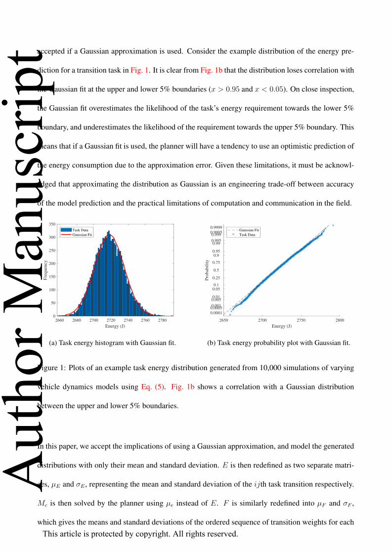
accepted if a Gaussian approximation is used. Consider the example distribution of the energy pre-

diction for a transition task in Fig. 1. It is clear from Fig. 1b that the distribution loses correlation with

the Gaussian fit at the upper and lower 5% boundaries (x > 0.95 and x < 0.05). On close inspection,

the Gaussian fit overestimates the likelihood of the task’s energy requirement towards the lower 5%

boundary, and underestimates the likelihood of the requirement towards the upper 5% boundary. This

means that if a Gaussian fit is used, the planner will have a tendency to use an optimistic prediction of

the energy consumption due to the approximation error. Given these limitations, it must be acknowl-

edged that approximating the distribution as Gaussian is an engineering trade-off between accuracy

of the model prediction and the practical limitations of computation and communication in the field.

2660 2680 2700 2720 2740 2760 2780

Energy (J)

0

50

100

150

200

250

300

350

Fre

qu

ency

Task Data

Gaussian Fit

(a) Task energy histogram with Gaussian fit.

2650 2700 2750 2800

Energy (J)

0.0001

0.00050.001

0.005 0.01

0.050.1

0.25

0.5

0.75

0.90.95

0.990.995

0.999 0.9995

0.9999

Pro

bab

ilit

y

Gaussian Fit

Task Data

(b) Task energy probability plot with Gaussian fit.

Figure 1: Plots of an example task energy distribution generated from 10,000 simulations of varying

vehicle dynamics models using Eq. (5). Fig. 1b shows a correlation with a Gaussian distribution

between the upper and lower 5% boundaries.

In this paper, we accept the implications of using a Gaussian approximation, and model the generated

distributions with only their mean and standard deviation. E is then redefined as two separate matri-

ces, µE and σE , representing the mean and standard deviation of the ijth task transition respectively.

Mc is then solved by the planner using µe instead of E. F is similarly redefined into µF and σF ,

which gives the means and standard deviations of the ordered sequence of transition weights for each

Aut

hor M

anus

crip

t


vehicle respectively.

The stochastic energy prediction, H , is defined as a random variable pertaining to the task, plan or

battery capacity as follows:

H ∼ N (µ, σ2) (7)

Ht ∼ N (µFi , σFi2) (8)

Hp ∼ N (∑

µF ,∑

σF2) (9)

Hb ∼ N (µeb , σeb2) (10)

where Ht is the energy prediction for a particular task, Hp is the energy prediction for the summation

of tasks to be performed, and Hb is a random variable obtained based on battery discharge/recharge

data.

2.2.1 Naive Energy Consumption Certainty Estimation

The vehicle is equipped with sensors to measure the voltage and current consumption close to the

battery terminals. The measured energy consumption of the vehicle is calculated by performing

numerical integration using the trapezoidal rule of the measured power consumption over the time

interval ∆t = t(k)− t(k − 1):

Em(k) =Pm(k) + Pm(k − 1)

2∆t+ Em(k − 1) (11)

With the energy consumption prediction now represented as a Gaussian random variable (H), a simple

metric to determine the likelihood that the vehicle has consumed more than the prediction is the

survival function:

Aut

hor M

anus

crip

t


SH(Em(k)) = P (H > Em(k)) = 1−∫ Em(k)

−∞

1√2πσ2

H

e− (x−µH )2

2σ2H dx (12)

The survival function metric allows the operator to specify a lower limit (δ) for the supervisor based

on the likelihood that Em(k) is not greater than H . If SH < δ, then the supervisor will activate a

recourse action behaviour. For δ > 0.5, the operator is encouraging the supervisor to be conservative

and activate recourse actions earlier and vice versa for δ < 0.5.

2.3 Recourse Actions

By implementing SH and the δ condition across different energy consumption scales, several levels

of decision making for the supervisor can be designed based on the expected operations of a deployed

vehicle. For example, when the vehicle switches to its own power supply, it must then keep track of

the energy consumed when compared to the estimated energy capacity of the vehicle, eb. When the

supervisor commences a plan given to it by the mission planner, it must compare the energy consumed

against the predicted total energy consumption of the plan. Finally, each plan is a sequence of tasks,

each of which should be considered on the task energy prediction scale.

To formalise this we defined separate datum points for the battery, plan, and task energy scales.

1. On vehicle power source mode switch to battery (battery datum), ob

2. On commencement of a plan (plan datum), op.

3. On commencement of a task (task datum), ot.

As the vehicle progresses through a mission, task Et, plan Ep, and battery Eb scales are simultane-

ously evaluated in the equations below.

Aut

hor M

anus

crip

t


Eb(k) = Em(k)− ob (13)

Ep(k) = Em(k)− op (14)

Et(k) = Em(k)− ot (15)

These energy measurements are then compared with their respective H energy predictions (Eqs. (8)

to (10)) based on the survival function activation criteria (Eq. (12)). As an additional fail-safe, we

also place a hard limit on the minimum measured voltage of the battery, Vlim. The recourse actions

and their activation conditions are listed below:

1. SHt(Et(k)) < δt: skip task heuristic.

2. SHp(Ep(k)) < δp: replan heuristic.

3. SHb(Eb(k)) < δb: return to rendezvous (home) position.

4. Vm(k) < Vlim: emergency power saving mode.

5. Otherwise: continue current plan.

The first and second recourse action activations are described in the following subsections. The third

activation commands the vehicle to travel to the home point. The fourth activation is an emergency

fail-safe mode triggered when the voltage of the battery has dropped below the minimum voltage

requirement of the thrusters. The vehicle shuts down the motors and is stranded.

2.3.1 Task Skip Heuristic

The task skip heuristic enables when the task survival function is below the task survival threshold.

The supervisor performs a naive linear estimate of the energy remaining for the current task, E ′T by:

Aut

hor M

anus

crip

t


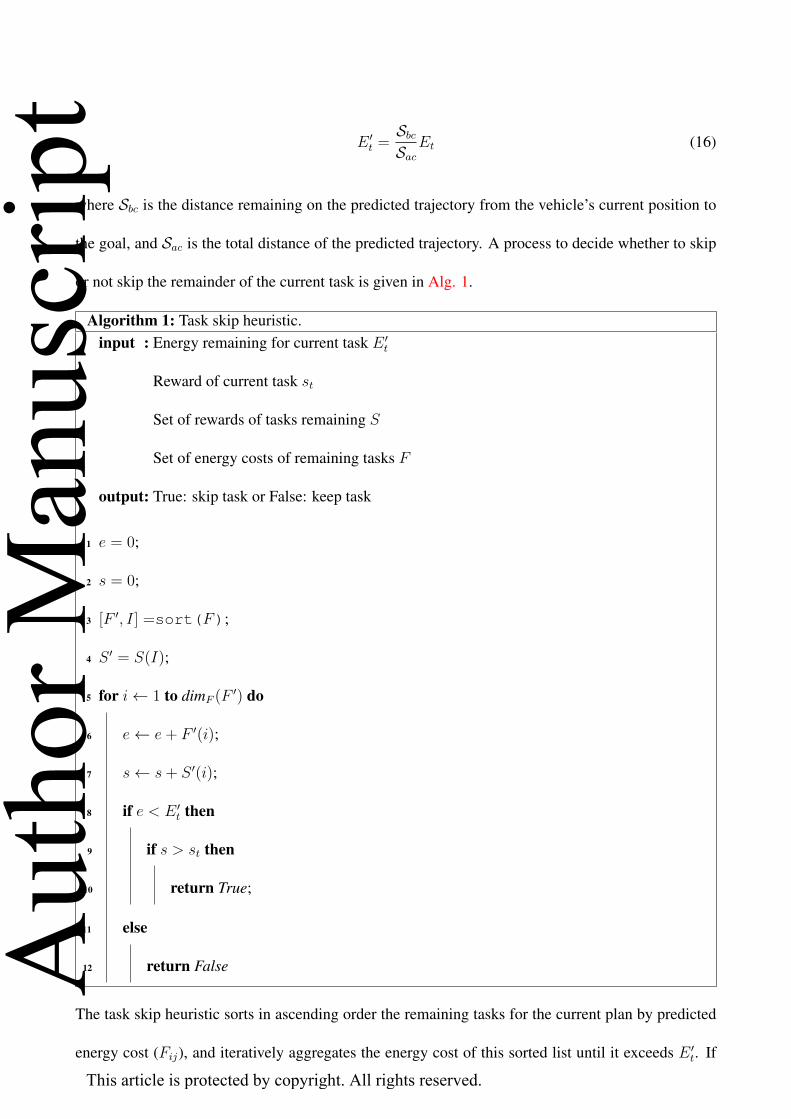
E ′t =SbcSac

Et (16)

where Sbc is the distance remaining on the predicted trajectory from the vehicle’s current position to

the goal, and Sac is the total distance of the predicted trajectory. A process to decide whether to skip

or not skip the remainder of the current task is given in Alg. 1.

Algorithm 1: Task skip heuristic.input : Energy remaining for current task E ′t

Reward of current task st

Set of rewards of tasks remaining S

Set of energy costs of remaining tasks F

output: True: skip task or False: keep task

1 e = 0;

2 s = 0;

3 [F ′, I] =sort(F);

4 S ′ = S(I);

5 for i← 1 to dimF (F ′) do

6 e← e+ F ′(i);

7 s← s+ S ′(i);

8 if e < E ′t then

9 if s > st then

10 return True;

11 else

12 return False

The task skip heuristic sorts in ascending order the remaining tasks for the current plan by predicted

energy cost (Fij), and iteratively aggregates the energy cost of this sorted list until it exceeds E ′t. If

Aut

hor M

anus

crip

t


the accumulated reward of the sorted, remaining tasks exceeds the reward for the current before this

condition then the algorithm returns true (i.e. skip the task). Otherwise the algorithm returns false

(i.e. keep the task).

2.3.2 Replan Action

During deployment, the vehicle keeps a track of the tasks that were completed and the tasks that

were skipped due to the task skip recourse action. Upon activation of the replan recourse action,

the vehicle first must determine if it can communicate with the first stage of the mission planner. If

communication is successful, it sends the request R to the mission planner, containing the following

information:

R = (C,D, E , L, E(k)) (17)

where C ⊂ R is the set of completed tasks, D ⊂ R is the set of skipped tasks, E is the set of final

energy measurements for each completed task (Et) and L is the location of the vehicle at the time

of replan request. Some of the elements in E will contain the consumed energy from tasks that were

skipped previous to it. The vehicle then holds its current position while the mission planner generates

a new solution from R and updates Mc. Once the vehicle receives the updated Mc, it begins the

new plan. If the vehicle is not within communication range, it activates the ’return home’ recourse

action. Ideally, the replanning recourse would happen entirely onboard the vehicle. However, due

to the computational constraints of current small form factor embedded computers that typically run

the software of AMVs, the replanning steps must be outsourced to an external computer (such as a

shoreside system) that can handle the planning requirements.

One potential method for enabling online replanning on a low-cost embedded system would be to

create a lightweight planning agent that only uses the task information given in the original plan to

Aut

hor M

anus

crip

t


generate a replan solution. This means that not all potential tasks will be considered, but the vehicle

would then be able to create a new plan based on a subset of the old. This also ensures, in a multi-

AMV deployments, that each vehicle would be guaranteed not to create conflicts with other vehicles

by allocating itself an already allocated task. This comes with the caveat of restricting each vehicle’s

knowledge of the global mission state, meaning that vehicles will be unable to act on tasks that

weren’t initially given to them. This increases the risk of mission failure due to local vehicle failures.

A distributed planning architecture, such as described in Zlot (2006) and Sotzing et al. (2007), would

enable vehicles to actively give, take and swap tasks according to their replan actions.

Upon receiving R from the vehicle, the first stage planner formulates a new Mo based on the tasks

in the old Mc that were neither skipped nor completed. This reduces the size of E that has to be

searched through, because the rows and columns of the previous E that reference starting from, or

moving to completed or skipped tasks can be deleted. The energy constraint (eb from Eq. (6)) is

replaced with the previous plan’s energy prediction minus the energy consumed during deployment

(replace eb with µHp − E(k) in Eq. (6)). Additionally, the planner must redefine E1j and Ei1 with an

energy distribution prediction based on the provided L, which is the new starting point of the vehicle

in the new plan. By reducing the size of E and only performing Monte Carlo simulation on the subset

of trajectories that start at L, the replanning process time is a fraction of the initial plan generation

time.

3 System Description

The full system is comprised of two components: the shoreside mission planner and Human-Machine

Interface (HMI), and the ASV1. The shoreside systems and ASV communicate with each other over1The ASV system framework is open-source and has been made available at https://github.com/

FletcherFT/asv_framework

Aut

hor M

anus

crip

t


https://github.com/FletcherFT/asv_framework

https://github.com/FletcherFT/asv_framework

a Wi-Fi network, with a Radio Controller (RC) included as a manual override backup. Both systems

were built using the Robot Operating System (ROS) middleware.

3.1 Shoreside Subsystem

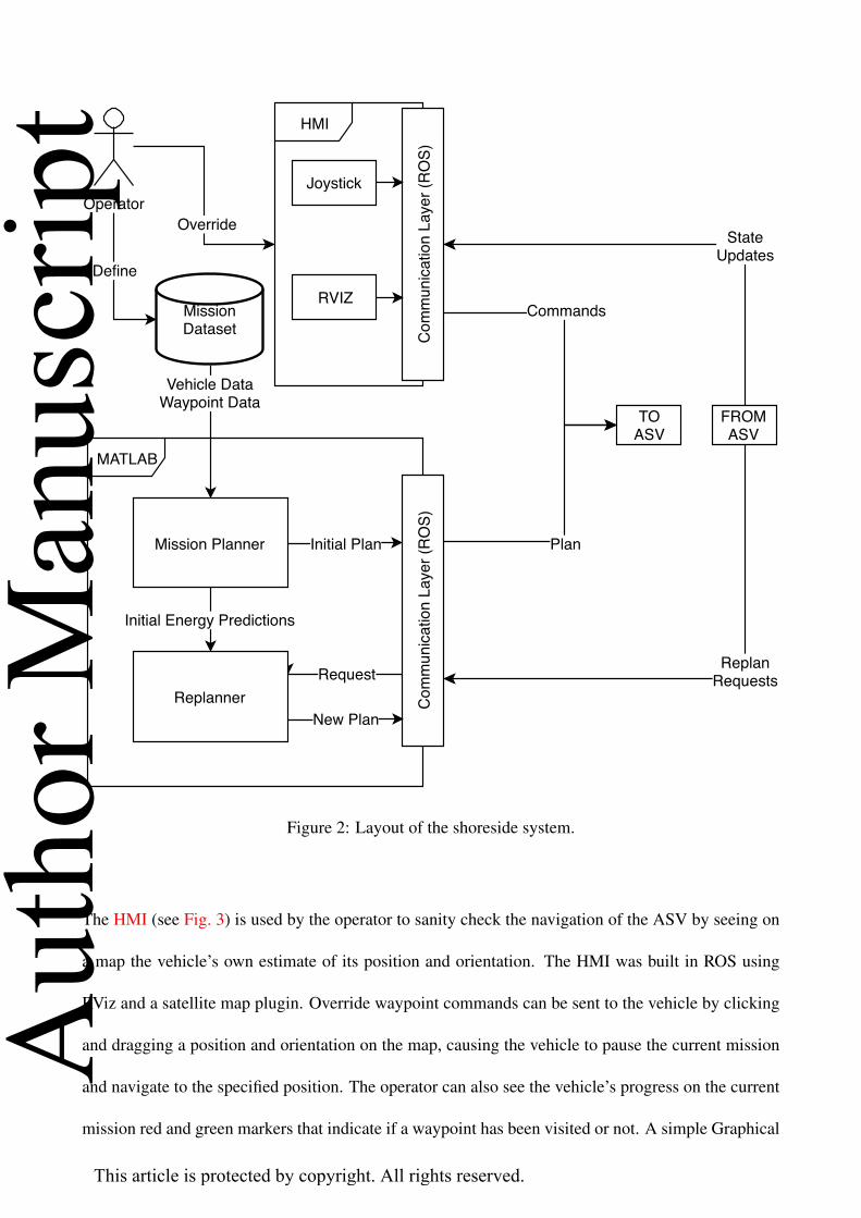
Fig. 2 depicts the major components of the shoreside system. The first stage of the mission planner

described in Sections 2.1 to 2.2 was developed in MATLAB and extended with the robotics system

toolbox to allow it to interface with the ROS network. The operator provides the mission planner

with T and V , and the mission planner computes an optimal plan that it sends to the ASV via a

ROS message. During mission run-time, the planner listens for planning requests from the ROS

communication layer.

Aut

hor M

anus

crip

t


Vehicle DataWaypoint Data

MissionDataset

Define

OverrideOperator

MATLAB

Request

Plan

Com

mun

icat

ion

Laye

r (R

OS)

Initial Plan

Initial Energy Predictions

Mission Planner

New PlanReplanner

HMI

Commands

Com

mun

icat

ion

Laye

r (R

OS)

Joystick

RVIZ

TOASV

StateUpdates

ReplanRequests

FROMASV

Figure 2: Layout of the shoreside system.

The HMI (see Fig. 3) is used by the operator to sanity check the navigation of the ASV by seeing on

a map the vehicle’s own estimate of its position and orientation. The HMI was built in ROS using

RViz and a satellite map plugin. Override waypoint commands can be sent to the vehicle by clicking

and dragging a position and orientation on the map, causing the vehicle to pause the current mission

and navigate to the specified position. The operator can also see the vehicle’s progress on the current

mission red and green markers that indicate if a waypoint has been visited or not. A simple Graphical

Aut

hor M

anus

crip

t


User Interface (GUI) to send start/pause mission commands, calibration commands to the navigation

system, and Proportional Integral Derivative (PID) tuning commands to the control system was also

implemented.

Figure 3: Screenshot from the HMI component of the shoreside system. The vehicle’s position and

orientation is provided by the red/green/blue axis, incomplete waypoints are shown as red spherical

markers, completed tasks are shown in green. The selected waypoint for completion is shown with a

red marker and fuchsia arrow.

3.2 ASV Subsystem

A simple model-scale box-barge hull was converted into a prototype autonomous platform for the

purposes of testing planning, guidance, navigation and control algorithms. The vehicle, pictured in

Fig. 4, has three actuators: one tunnel thruster located towards the bow and two azimuth thrusters

located at the transom. This configuration means the vehicle can move independently in forwards

(surge), sideways (sway), and heading (yaw) motions. To take advantage of this, an autopilot and a

dynamic positioning controller were designed to control the vehicle in two different operating modes:

Aut

hor M

anus

crip

t


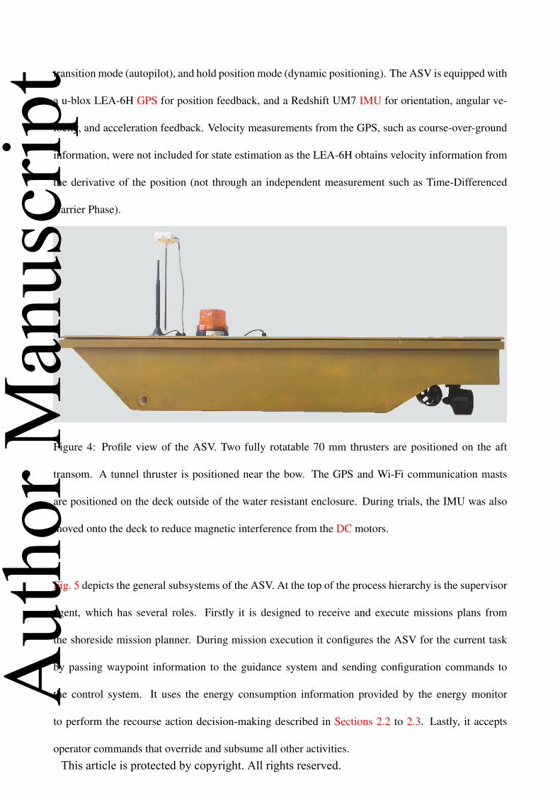
transition mode (autopilot), and hold position mode (dynamic positioning). The ASV is equipped with

a u-blox LEA-6H GPS for position feedback, and a Redshift UM7 IMU for orientation, angular ve-

locity, and acceleration feedback. Velocity measurements from the GPS, such as course-over-ground

information, were not included for state estimation as the LEA-6H obtains velocity information from

the derivative of the position (not through an independent measurement such as Time-Differenced

Carrier Phase).

Figure 4: Profile view of the ASV. Two fully rotatable 70 mm thrusters are positioned on the aft

transom. A tunnel thruster is positioned near the bow. The GPS and Wi-Fi communication masts

are positioned on the deck outside of the water resistant enclosure. During trials, the IMU was also

moved onto the deck to reduce magnetic interference from the DC motors.

Fig. 5 depicts the general subsystems of the ASV. At the top of the process hierarchy is the supervisor

agent, which has several roles. Firstly it is designed to receive and execute missions plans from

the shoreside mission planner. During mission execution it configures the ASV for the current task

by passing waypoint information to the guidance system and sending configuration commands to

the control system. It uses the energy consumption information provided by the energy monitor

to perform the recourse action decision-making described in Sections 2.2 to 2.3. Lastly, it accepts

operator commands that override and subsume all other activities.

Aut

hor M

anus

crip

t


The lower levels of the ASV system are centered around the Guidance, Navigation and Control

paradigm described in Fossen (2011a). The navigation module consists of drivers for reading the

GPS and IMU, and an Extended Kalman Filter (EKF) state estimator. The EKF is based on a

2D constrained general point kinematic model described in Moore and Stouch (2014). It fuses

the GPS and IMU measurements into an estimate of the vehicle’s position (in Universal Trans-

verse Mercator (UTM) coordinates), orientation (following an East-North-Up convention), and an-

gular and linear velocities in the body-frame of the vehicle (following a Forward-Port-Up conven-

tion). The chosen framing conventions differ from the marine robotics standard of using North-

East-Down/Forward-Starboard-Down because the core ROS coordinate system operates by default in

East-North-Up/Forward-Port-Up.

VehicleSystem

ReplanRequest

PositionOrientation

Duration

Supervisor

State Navigation Guidance

Control

ControllerConfiguration

Energy Aggregate

Energy Monitor

Sample VoltageCurrent

Power DistributionMotors

Override

PlanReplan

Request

State Updates

Com

mun

icat

ion

Laye

r (R

OS)

TOHMI

PlanFROMMP

TOMP

CommandsFROMHMI

Figure 5: Subsystem layout of the ASV.

Aut

hor M

anus

crip

t


The guidance module uses the Line of Sight (LOS) guidance controller from Fossen (2011b) with a

custom piecewise function (Eq. (20)) to provide speed and heading errors for the control module to

regulate to zero. The guidance distance and heading error, D and ψe are:

D =√

(xd − x)2 + (yd − y)2 (18)

ψe = atan2(yd − y, xd − x)− ψ (19)

where the terms are depicted in Fig. 6.

The autopilot component within the control module requires a forward speed error, which is calculated

in the guidance module as follows:

ud(D, ra, ψe) =

0 D ≤ ra

0 |ψe| > π5

U D > ra, |ψe| ≤ π5

(20)

ue = ud − u (21)

where ra is the radius of acceptance (i.e. the maximum distance the vehicle can be from the waypoint).

U is a forward speed setpoint that the operator specifies in Iv. Eq. (20) contains conditional setpoint

changes to slow the vehicle down and reduce its turning circle for large guidance heading errors

(arbitrarily defined as anything larger than π5

radians), and to stop the vehicle entirely when it has

reached the radius of acceptance for the waypoint. When the waypoint is reached, the guidance

module requests a new waypoint from the supervisor or idles if there is none.Aut

hor M

anus

crip

t


N

E

ψd

( , )xd yd

ψ

(x, y)

ψe

− xxd

− yyd

u

v

D

xb

ra

yb

Figure 6: Geometry that the LOS guidance controller uses to calculate the autopilot and dynamic

positioning controller errors. The autopilot error signals depend on ψe and D. The dynamic position-

ing error signals depend on xb, yb, and ψd. The red lines are the projection of the ASV body-frame

coordinates onto the position errors, which are used to calculate xb and yb.

When the ASV is in dynamic positioning mode, the guidance module provides the control module

with longitudinal and transverse position errors by rotating the inertia-frame components of D into

the body-frame:

Aut

hor M

anus

crip

t


R =

− sinψ 0 0

0 sinψ 0

0 0 1

(22)

yb

xb

ψb

= R

xd − x

yd − y

ψd − ψ

(23)

where xb and yb are the body-frame position errors as depicted in Fig. 6. ψb is the error between the

desired vehicle heading and the current vehicle heading.

The control module consists of an autopilot controller, a dynamic positioning controller, and a con-

trol allocation algorithm. The autopilot and dynamic positioning controllers regulate the speed and

heading, and position and heading respectively by outputting a vector of commanded body forces in

the surge and sway directions, and a yawing moment (τ c). The autopilot controller is a multi-input,

multi-output PID controller that outputs τ c as:

τ cX = Kpue +Ki

∫ue dt+Kd

duedt

(24)

τ cY = 0 (25)

τ cNZ = Kpψe +Ki

∫ψe dt+Kd

dψedt

(26)

The transverse velocity is not regulated, which can cause the vehicle to drift sideways when turning.

The dynamic positioning controller calculates τ c through the following:Aut

hor M

anus

crip

t


τ cX = Kpxb +Ki

∫xb dt+Kd

dxbdt

(27)

τ cY = Kpyb +Ki

∫yb dt+Kd

dybdt

(28)

τ cNZ = Kpψb +Ki

∫ψb dt+Kd

dψbdt

(29)

where ψd is the desired heading for the vehicle.

The control allocation algorithm is a quadratic programming solver formulated as the constrained

fixed-angle thruster allocation problem described in Fossen (2011c). Although the thrusters are fully

rotatable, power consumption can be reduced by ensuring that the azimuth thrusters only rotate when

the supervisor switches the control mode from autopilot to dynamic positioning (or vice versa). Two

thruster configurations were defined for each control mode. When in autopilot mode, the thrusters are

oriented parallel to the longitudinal axis of the ASV. When in dynamic positioning mode, the thrusters

are swivelled ±45◦ to either side of the longitudinal axis. The control allocation solution yields both

the commanded thrusts for each thruster, and the achieved body forces and yawing moment provided

by the solution (τa). The commanded thrusts are converted to a vector of electronic speed controller

duty cycles (d), which are outputted to the motor drivers for each respective thruster.

4 Energy Forecasting

In Section 2.2.1 a naive method was presented that calculated a survival metric based on the ag-

gregated energy measurements. Through this method the operator safeguards against the future by

providing a margin of safety on the survival thresholds, making the supervisor trigger recourse actions

according to the likelihood that the vehicle has used the planned energy for a task, plan, or the battery.

One issue with this is that the recourse decision is made at the time of the energy measurement and

runs the risk of being activated too late. A forecasting approach could be used in situ to predict ahead

Aut

hor M

anus

crip

t


of time if a survival threshold will be crossed, allowing the supervisor to initiate recourse actions

earlier and save energy in the process.

Forecasting the power consumption of the vehicle is a three-stage forecasting process that requires:

1. Prediction of the vehicle’s kinematics.

2. Prediction of the vehicle’s control response for a given task and kinematic state.

3. Prediction of the vehicle’s power consumption given the control response of the vehicle.

The following subsections detail a hybrid state prediction and control process, using data-driven ma-

chine learning models for the kinematic state and power consumption prediction, and classic PID

control processes for the control response calculations. A simplified block diagram summarising the

major stages of the process is provided in Fig. 7.

KinematicState

PredictionControlProcess

PowerPrediction

ControlOutput

PositionVelocity

TaskWaypoint

Figure 7: Simple view of the hybrid power prediction process. The first block predicts the new

kinematic state of the vehicle given the control output as external feedback. The second block receives

the new kinematic state and a waypoint reference from the task data and computes a control output.

The third block receives the new control output and predicts the power consumption of the vehicle.

The main feedback loop (i.e. setting k = k + 1) is coloured blue.Aut

hor M

anus

crip

t


4.1 Kinematic State Prediction

The ASV is expected to operate in an environment without large rolling, pitching, or heaving motions,

so the kinematics simplify to 3 degrees of freedom (two in translation, and one in rotation). The

kinematic state of the vehicle is defined as:

η = [x, y, ψ]T (30)

ν = [u, v, r]T (31)

where η is the vehicle’s position in the inertia-frame. In this case the x and y coordinates are the

vehicle’s latitude and longitude projected into UTM, and ψ is the vehicle’s heading relative to East

following a East-North-Up convention. ν is the ASV’s body-frame linear velocities in the longitudinal

(u) and transverse (v) directions and the angular turning rate in yaw (r). The vectorised kinetic model

for marine vehicles is:

τa = Mν̇ + (C(ν) + D(ν))ν + g(η)− τ e (32)

where τa is the vector of achieved body-fixed forces outputted by the controller in longitudinal and

transverse directions, and the commanded yawing moment. M is a matrix containing the summation

of the added mass and inertia terms of the vehicle. C(ν) is an array containing the summation of

the rigid body and added mass Coriolis and centripetal terms as a function of ν. D(ν) is a matrix

of hydrodynamic damping terms (i.e. the drag coefficients) as a function of ν. g is the vector of

hydrostatic forces according to the vehicle’s position and orientation within the water column. τ e is

the sum total of body-frame referenced environmental loads acting on the vehicle.

The vehicle’s kinematic states are predicted according to evaluation of the kinetic model in Eq. (32).

Aut

hor M

anus

crip

t


This is a complex process as both the manoeuvring loads and environmental loads are non-linear and

may not be able to be accurately observed in situ. The constant parameters in M, C, and D can be

identified through captive model testing of the vehicle, but must be updated if modifications to the

vehicle (such as payloads) are introduced. Calculation of τ e also requires sensing and observation of

the environment (wind, current, and waves) which this ASV is not equipped to perform.

An alternative to model-based kinematic state prediction is to perform supervised learning on col-

lected data to obtain an approximation of the Eq. (32). LSTM networks have seen success in learning

predictions from time series data in other domains, making it a good candidate for predicting the

trajectory and control time series data. The LSTM design in Fig. 8 performs the following operation:

νk+1 = f(νk, ψk, τak) (33)

where ψk and τak are chosen as additional explanatory variables. Due to the internal feedback na-

ture of the LSTM architecture, the network may also learn relationships between the change in and

aggregate of ν over time (ν̇ and η) but this is not guaranteed. ν̇ is not included as the measured

accelerations provided by the IMU are too noisy. The x and y components of η are also not included

as they are not bounded by upper and lower limits (unlike ψ which is bound between ±π radians),

which would make it harder for the LSTM to generalise.

Aut

hor M

anus

crip

t


��

��

��

� +1... ......

Input Layer Fully ConnectedHidden Layer LSTM Hidden Layer

Fully ConnectedLayer with 50%

dropoutOutput Layer

Figure 8: Network layout of the ν state prediction LSTM. The network accepts the current body

velocity vector νk, the current yaw heading ψk, and the achieved vector of body forces τak. The

network consists of a latent space hidden layer, the LSTM layer, another fully connected layer with a

50% dropout to reduce the chance of overfitting, and then the output layer (which is νk+1).

4.2 Power Consumption Prediction

As discussed in Section 2.1, the power consumption of the ASV depends upon the commanded

thruster outputs, the hotel load, and the efficiency of the electrical distribution system. Identifica-

tion of each of these contributors can provide a good estimate of the total power consumption of the

vehicle. However, complex transient effects that occur on the distribution system during changes in

thruster output, and the effect of hydrodynamic loading on the thrusters during changes in output are

not typically modelled. Once again, a data-driven approach using an LSTM network (see Fig. 9) may

be able to capture these effects.

Aut

hor M

anus

crip

t


��

+1

� +1... ......

Input Layer Fully ConnectedHidden Layer LSTM Hidden Layer

Fully ConnectedLayer with 50%

dropoutOutput Layer

Figure 9: Network layout of the power prediction LSTM. The network accepts the current power Pk

and the predicted commanded duty cycles of the thrusters from the control allocation block (dk+1).

The network consists of a latent space hidden layer, the LSTM layer, another fully connected layer

with a 50% dropout to reduce the chance of overfitting, and then the output layer (which is Pk+1).

The power prediction network performs the following operation:

Pk+1 = f(Pk,dk+1) (34)

where dk+1 is the vector of commanded duty cycles for all thrusters as outputted by the control

process prediction. Duty cycle was selected over force because duty cycle is bounded between 0 and

1, making it easier for the LSTM to generalise.Aut

hor M

anus

crip

t


4.3 Hybrid Energy Forecaster Model

The kinematic state of the vehicle is used by the control process outlined in Section 3 to obtain the

achieved body forces to regulate the kinematic state to specific set points that reach the task waypoint

following the LOS guidance controller. Fig. 10 shows the full process of the hybrid energy forecast

model. The ν prediction LSTM first predicts the body-frame velocities of the vehicle at k + 1. Then

νk+1 is integrated and transformed into the inertia frame to obtain ηk+1. The task waypoint, νk+1,

and ηk+1 are inputted into the LOS guidance controller to obtain the forward speed error, uek+1, and

the LOS heading error, ψek+1.

The autopilot controller functions as described in Eqs. (24) to (26). The gains for the controllers are

copied from the gains used in the ASV control system. The autopilot controller outputs the vector of

desired body forces and moments (τ ck+1), which is then inputted into a copy of the ASV’s control

allocation process. The control allocation process outputs the achieved body forces and moments,

τak+1, which is fed back into the ν prediction LSTM. The duty cycles for the thrusters, dk1 , is also

calculated by the control allocation process and is used by the power prediction LSTM to obtain Pk+1.

τak+1 is fed back into the ν prediction LSTM for the next prediction cycle. The energy forecast can

then be computed by aggregating the forecast power from Eq. (34) substituted into Eq. (11).

Aut

hor M

anus

crip

t


νk

ψk

τa k

(LST

M 1

)

→ν

kν

k+1

∫

η˙k+1

()

Jb

od

y

wo

rldη

k+1

rk+1

νk+1

+Δψ

LOS

Gui

danc

e

Task

Auto

pilo

tC

ontro

ller

+∫

ηk

ηk+1

Δη

Con

trol

Allo

catio

n(L

STM

2)

→P

kP

k+1

νk+1

ηd k+1

ψk

ψk+1

ue k+1

ψe k+1

τc k+1

τa k+1

Pk+1

dk+1

Figu

re10

:Fu

llbl

ock

diag

ram

ofth

ehy

brid

LST

M/c

ontr

olpr

oces

spo

wer

fore

cast

er.

Theν

stat

epr

edic

tion

LST

Mpr

oduc

esνk+1

pred

ictio

nsw

hich

are

then

tran

sfor

med

toth

ein

ertia

fram

ean

din

tegr

ated

toob

tain

the

vehi

cle’

scu

rren

tpos

ition

,aL

OS

guid

ance

func

tion

calc

ulat

esth

ese

tpoi

ntfo

rth

e

forw

ard

spee

dco

ntro

ller

and

the

rela

tive

bear

ing

erro

r,w

hich

feed

sin

toth

eau

topi

lotc

ontr

olle

r.T

heau

topi

loto

utpu

tsa

com

man

ded

body

forc

ean

d

mom

entv

ecto

rτck+1

toth

eco

ntro

lallo

catio

nal

gori

thm

,whi

chde

term

ines

the

duty

cycl

efo

rea

chth

rust

er(d

k+1).

Fina

llyth

epo

wer

pred

ictio

nL

STM

uses

the

pow

erfr

omth

ecu

rren

tste

pPk

and

the

pred

icte

dth

rust

erdu

tycy

cledk+1

topr

edic

tPk+1.T

hebl

uelin

esin

dica

teth

efe

edba

ckpa

ths

whe

rek

is

sett

ok

+1

fort

hene

xttim

est

ep.

Aut

hor M

anus

crip

t


5 Results of Field Trials and Energy Forecasting

Fig. 11 details the mission data sets that were generated within a Geographic Information System

package. The close, medium, and long range missions were specified as collections of waypoints

with no specific order (T from Section 2.1). The rectangle mission has a human-defined order as

it is a calibration test for the ASV’s autopilot controller. Each mission was run several times with

varying δp and δt thresholds, which are the primary criteria used by the supervisor for making in situ

decisions. Weather data was obtained from Bureau of Meteorology (2018) during post-processing

of the data. Section 5.1 presents two example runs where the behaviour of the vehicle is drastically

different due to the manipulation of these thresholds.

_̂

5 m 10 m 20 m 40 m80 m

120 m

Source: Esri, DigitalGlobe, GeoEye, Earthstar Geographics, CNES/Airbus DS, USDA, USGS,AeroGRID, IGN, and the GIS User Community

Ranges_̂ Home Position

Shoreside LocationRectangle MissionClose Range MissionMedium Range MissionLong Range Mission

Wind (km/h)

Figure 11: Summary of mission datasets generated for Lake Waverley. All missions except for the

rectangle mission are not given a sequence by the operator. The mission planner creates a sequence

during plan generation. Wind data was obtained from a local weather station 5 km from the lake,

providing twice-daily measurements.

Aut

hor M

anus

crip

t


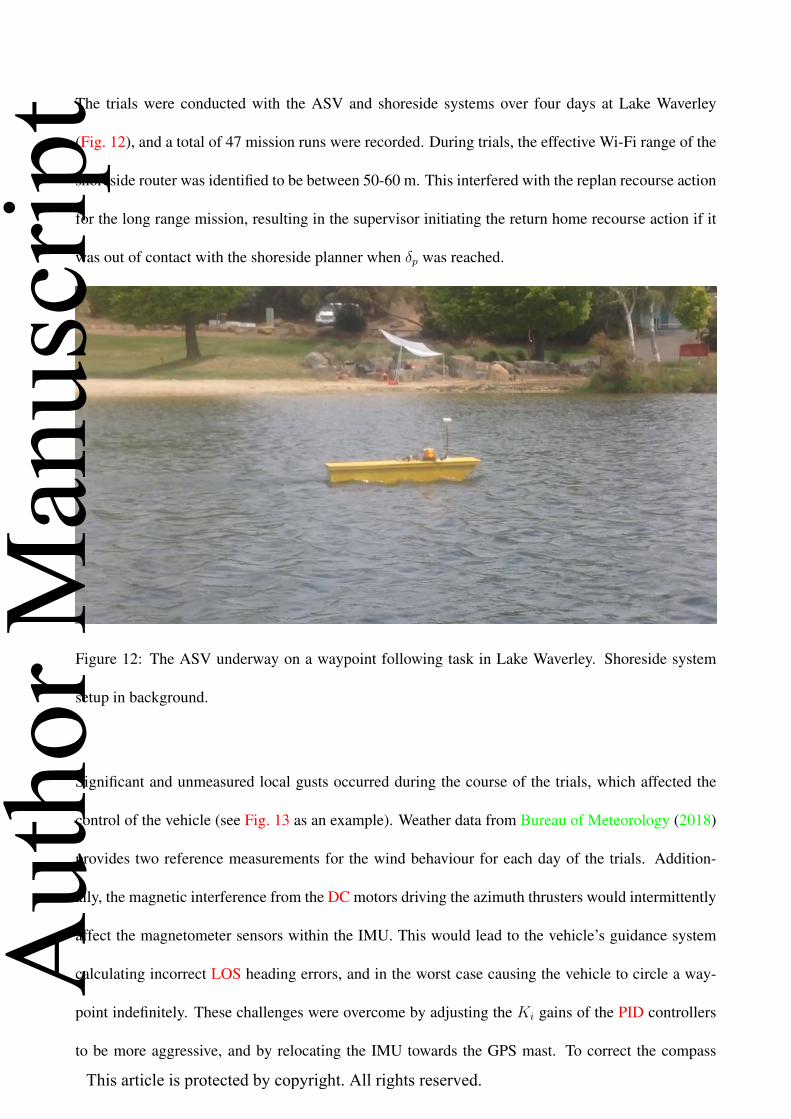
The trials were conducted with the ASV and shoreside systems over four days at Lake Waverley

(Fig. 12), and a total of 47 mission runs were recorded. During trials, the effective Wi-Fi range of the

shoreside router was identified to be between 50-60 m. This interfered with the replan recourse action

for the long range mission, resulting in the supervisor initiating the return home recourse action if it

was out of contact with the shoreside planner when δp was reached.

Figure 12: The ASV underway on a waypoint following task in Lake Waverley. Shoreside system

setup in background.

Significant and unmeasured local gusts occurred during the course of the trials, which affected the

control of the vehicle (see Fig. 13 as an example). Weather data from Bureau of Meteorology (2018)

provides two reference measurements for the wind behaviour for each day of the trials. Addition-

ally, the magnetic interference from the DC motors driving the azimuth thrusters would intermittently

affect the magnetometer sensors within the IMU. This would lead to the vehicle’s guidance system

calculating incorrect LOS heading errors, and in the worst case causing the vehicle to circle a way-

point indefinitely. These challenges were overcome by adjusting the Ki gains of the PID controllers

to be more aggressive, and by relocating the IMU towards the GPS mast. To correct the compass

Aut

hor M

anus

crip

t


misalignment fault the mission had to be paused and manual override commands were given to the

vehicle to align its heading with an external measurement of magnetic north so that the navigation

system’s compass datum could be reset. The effects of both the wind and the magnetic interference

will also be important in Section 5.2.

_̂

5 m 10 m 20 m 40 m80 m

120 m


Ranges_̂ Home Position

Shoreside LocationRectangle MissionActual TrajectoryAcceptance

Wind (km/h)

Figure 13: One of the rectangle missions performed by the ASV. Strong and intermittent North-

Westerly gusts blew the vehicle sideways from the expected trajectory, leading to trajectories with

cross-track errors that are sometimes large and sometimes small. The autopilot controller does not

control motion in the sway direction, leading to arcs in the achieved trajectory.

5.1 Recourse Action Effects

Adjusting the δ thresholds for each of the survival functions produces significantly different be-

haviours from the supervisor. Combinations of different thresholds result in behaviours where it

is difficult to identify which threshold contributes what to the result. To see the direct effects of δp

and δt as they operate independently, this section looks at two runs of the medium size mission: one

Aut

hor M

anus

crip

t


where δp is high and δt is off (i.e. < 0), and one where δt is high and δp is off.

Fig. 14 presents a run of the medium size mission with δt = −1e10−9 and δp = 0.85. From the

trajectory of the ASV, it appears that the ASV attempts to finish the waypoint tasks in the order

specified by the planner. When the threshold is crossed, the ASV performs a hold position manoeuvre

and requests a new plan from the shoreside planner. The new plan budgets in one waypoint task before

sending the vehicle to the home position. This behaviour is similar to the return home recourse actions

described in Evers et al. (2014) and Shang et al. (2016), but is capable of planning in tasks that are

along the route home.

!(

!(

!(

!(

!(

!(

!( !(

!(

!(

!(

!(!(

!(

!(

!(!(

!(

!(

!(

!(

!(

!(

!(

_̂

5 m10 m20 m

40 m

80 m


_̂ Home!( Completed M07

New Plan!( After Replan!( Hold Position

Trajectory M07Ranges

!( Incomplete!( Shoreside Location

Planned Medium Range MissionAcceptance M07

1.2.

3.4.

5.6.7. 8.

9.

# Time (s) Description1.-5. 35-181 Completed Task6. 203 Request Replan7. 300 Receive New Plan8. 326 Completed Task9. 387 Finish Mission

Events Log

Wind (km/h)

Figure 14: Progression of medium range mission 7. δp = 0.85 and δt = −1e10−9.

Fig. 15 presents the corresponding time series of battery, plan, and task survival function data for

medium mission 7. The vehicle fell out of contact with the mission planner after it had successfully

made a replan request, leading to a long hold position action. Once contact was reestablished, the

vehicle proceeded on the new mission and completed it without triggering a new replan recourse

Aut

hor M

anus

crip

t


action. The task survival function has drastic falling edges after a few seconds of performing a new

task. This indicates that the planner is underestimating the energy cost of performing tasks, and also

that the calculated Ht distributions have a small variance.

0 50 100 150 200 250 300 350 400

Time Since Mission Start (s)

0.96

0.98

1

0 50 100 150 200 250 300 350 400


0.85

0.9

0.95

1

0 50 100 150 200 250 300 350 400


0

0.5

1

1.-5.

6.

7.

8.

9.

Figure 15: Survival functions of medium range mission 7. The numbered arrows correspond to the

events log in Fig. 14. Task survival (δt) indicates that the generated plan is underestimating the power

consumption of the vehicle. The gap in time (between 200-300 s) is because the survival functions

are not considered by the supervisor while holding position.

As a basis of comparison, Fig. 16 presents run 22 of the medium range mission where δt = 0.5 and

δp = −1e10−9. The trajectory shows that the supervisor has a very short tolerance on pursuing a task

before skipping it and moving on to the next. The vehicle was only able to complete tasks where its

distance ended up being significantly closer than what was originally planned for it by virtue of the

Aut

hor M

anus

crip

t


task skip heuristic.

!(

!(

!(

!(

!(

!(

!(

!(

!(

!(

!(

!(

!(

!(!(

!(_̂

5 m10 m20 m

40 m

80 m


_̂ Home!( Skipped M22!( Completed M22

Trajectory M22Ranges

!( Shoreside LocationPlanned Medium Range MissionAcceptance M22

# Time (s) Description1. 17 Completed Task2.-7. 26-101 Skipped Task8.-9. 104-116 Completed Task10.-13. 129-176 Skipped Task14. 198 Completed Task15. 232 Finish Mission

Events Log

1.2.3.4.5.6.

7.8.9.

10.11.12.13.14.

15.Wind (km/h)

Figure 16: Medium range mission 22 progression. δt = 0.5 and δp = −1e10−9.

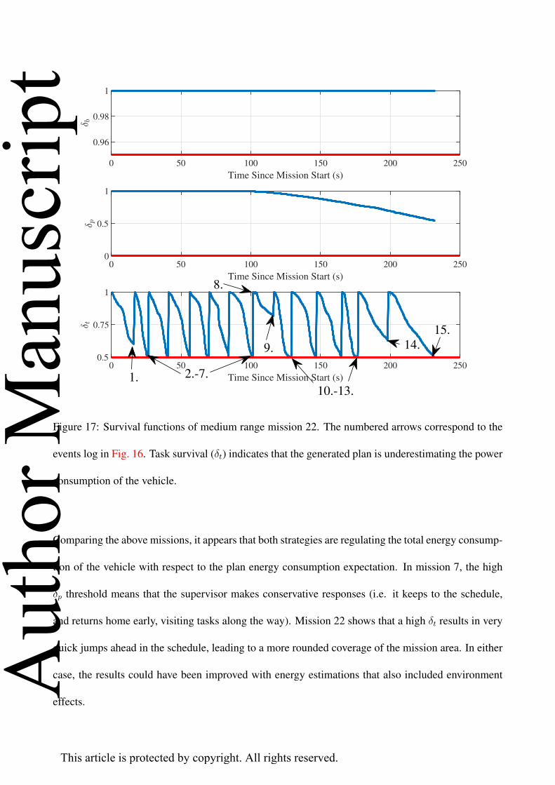
The survival functions for mission 22 are slightly different from mission 7. Fig. 17 shows that the

task survival function began decaying almost immediately after the task was initiated. This is likely

due to the more aggressive PID tunings and control output limits that were used on this run compared

to mission 7. The controller outputted higher thrust commands to the thrusters, which results in much

higher power consumption. The plan survival function also finishes quite close to 0.5, indicating that

the vehicle finished the mission close to the expected energy consumption of the plan.

Aut

hor M

anus

crip

t


0 50 100 150 200 250


0.96

0.98

1

0 50 100 150 200 250


0

0.5

1

0 50 100 150 200 250


0.5

0.75

1

1.

8.

9.

10.-13.

2.-7.

14.

15.

Figure 17: Survival functions of medium range mission 22. The numbered arrows correspond to the

events log in Fig. 16. Task survival (δt) indicates that the generated plan is underestimating the power

consumption of the vehicle.

Comparing the above missions, it appears that both strategies are regulating the total energy consump-

tion of the vehicle with respect to the plan energy consumption expectation. In mission 7, the high

δp threshold means that the supervisor makes conservative responses (i.e. it keeps to the schedule,

and returns home early, visiting tasks along the way). Mission 22 shows that a high δt results in very

quick jumps ahead in the schedule, leading to a more rounded coverage of the mission area. In either

case, the results could have been improved with energy estimations that also included environment

effects.Aut

hor M

anus

crip

t


5.2 Forecaster Evaluation

5.2.1 Training

The data collected during the Waverley trials was used to train the hybrid energy forecaster model.

During each mission the ASV switches between several operating modes: manual RC, autopilot, dy-

namic positioning, and idle. The power prediction LSTM was trained on data from each operating

mode, whereas the ν prediction LSTM was trained on the subset of the data where the vehicle was

operating in autopilot mode. The choice to only evaluate the ν LSTM on only the autopilot data was

made to simplify the controller component of the hybrid energy forecaster model. Forecasting the

control input of an operator’s RC command is counterintuitive, and forecasting the power consump-

tion of a vehicle in idle mode simplifies to forecasting the hotel load. The controller component could

be expanded to include the dynamic positioning controller in the future.

The data was split 9:1 between training and test data sets. Fig. 18a presents the training curve for

the ν prediction LSTM. Fig. 18b presents the Root-Mean-Squared Error (RMSE) of the trained ν

prediction LSTM in performing one-step predictions on the test data sets. The performance on the

test set indicates that the error in position between the predicted and actual will grow due to the

integration of the velocity error.

Aut

hor M

anus

crip

t


0 0.5 1 1.5 2

Iterations 104

2

4

6

8

Opti

mis

er L

oss

0 0.5 1 1.5 2

Iterations 104

1

2

3

4

RM

SE

0 0.5 1 1.5 2

Iterations 104

10-4

(a) ν Training Curve.

u (m/s) v (m/s) r (rad/s)

0

0.05

0.1

0.15

0.2

0.25

0.3

RM

SE

(b) ν Test RMSE Results.

Figure 18: Training performance of the ν prediction LSTM (Fig. 18a) and the one-step prediction

performance of the trained ν prediction LSTM on the test data set (Fig. 18b). The top and middle

plots of Fig. 18a are the optimisation loss and standardised RMSE (including a red moving mean

trend). The bottom plot is the learning rate, which is progressively halved during training.

5.3 Forecasting Kinematic State

To evaluate the forecast effectiveness, the trained predictor is first ’charged’ with feed-in data from

the test set. The length of the feed-in data does effect the quality of the forecast as the LSTM will

have more valid historical data available, but a trade-off has to be made with computational resources

(i.e. more memory is needed to store longer feed-in). The first 5 seconds of each of the test input

sets were reserved for feed-in (we found 5 seconds to be sufficiently long enough for the forecaster to

produce accurate forecasts).

Fig. 19 presents the error in distance-to-target between the actual and forecast for each autopilot task

(each coloured line representing a task). For positive D(t) − D̂(t), the forecasted vehicle position

is closer to the target than actual (optimistic forecast) and vice versa for negative D(t) − D̂(t) (pes-

simistic forecast). The error in ν between actual and forecast is integrated, which increases the rate

of error growth in forecasted η. This in turn affects the guidance module, which will use a different

Aut

hor M

anus

crip

t


distance-to-target to calculate the LOS heading error, ψe(t) (displayed in Fig. 20).

0 5 10 15 20 25 30

-10

-5

0

5

10

Figure 19: Error between actual and forecast distance to target over a 30 s window. The ν LSTM and

following autopilot controller were fed with 5 seconds of ground truth data before forecasting began.

In general, both the distance-to-target and the LOS heading error between forecasted and actual are

reasonably small for the first 5 seconds of forecasting. Some of the significant errors in Fig. 20 are be-

cause of strong wind gusts that occurred after forecasting began (i.e. the feed-in data did not indicate

enough information about the wind effects to the LSTM). In this respect we suggest extending the

kinematic LSTM by including wind speed and direction measurements as additional input variables.

This will allow the trained LSTM to learn a model for the estimation of τwind, improving the accu-

racy of the prediction. Including the next-step wind measurements as output variable would allow the

LSTM to make forecasts on future wind speed and direction. Reliable and frequent wind speed and

Aut

hor M

anus

crip

t


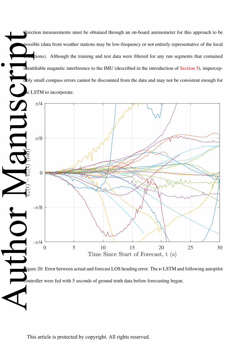
direction measurements must be obtained through an on-board anemometer for this approach to be

possible (data from weather stations may be low-frequency or not entirely representative of the local

conditions). Although the training and test data were filtered for any run segments that contained

identifiable magnetic interference to the IMU (described in the introduction of Section 5), impercep-

tibly small compass errors cannot be discounted from the data and may not be consistent enough for

the LSTM to incorporate.

0 5 10 15 20 25 30

- /4

- /8

0

/8

/4

Figure 20: Error between actual and forecast LOS heading error. The ν LSTM and following autopilot

controller were fed with 5 seconds of ground truth data before forecasting began.

Aut

hor M

anus

crip

t


5.4 Forecasting Energy

Fig. 21a presents the training curve for the power prediction LSTM. Fig. 21b presents the Root-Mean-

Squared-Error of the trained power prediction LSTM in performing one-step predictions on the test

data sets. The power prediction timeseries for the actual and forecast are integrated to obtain the

energy aggregate for each task, which is used for the rest of the forecast performance investigation.

0 100 200 300 400 500 600 700 800

Iterations

0.2

0.4

0.6

Opti

mis

er L

oss

0 100 200 300 400 500 600 700 800

Iterations

0.2

0.4

0.6

0.8

1

1.2

RM

SE

0 100 200 300 400 500 600 700 800

Iterations

6

8

1010-4

(a) Power training curve with optimiser loss (top),

RMSE (middle) and learning rate α (bottom).

P (W)

2

2.2

2.4

2.6

2.8

3

3.2

3.4

3.6

RM

SE

(b) Box and whisker plot of the Root-Mean-Squared-

Error between the test data and the power one-step

prediction of the LSTM.

Figure 21: Training and one-step prediction test results for the power prediction LSTM.

As soon as the forecast begins there is an error between the actual and forecast. To properly evaluate

the forecaster, some measurement for determining when the error is too large to be reliable (i.e. the

reliable forecast horizon) is required. A suitable candidate is the confidence interval of the planner-

generated energy distribution as this is based on what the Monte Carlo simulation and Gaussian

approximation produces for the given task. The 95% and 50% confidence offsets (i.e. 1.96 ± σ(k)

and 0.67 ± σ(k)) were chosen as standard reliability thresholds for the forecaster. The confidence

offsets were calculated by obtaining Eσ for a given Mo and plotting it with the total expected duration

of the task transition. Fig. 22 shows the 95% (1.96Eσ) and 50% (0.67Eσ) confidence offsets of the

Aut

hor M

anus

crip

t


distributions for the Monte Carlo simulated energy calculation of the all the potential tasks in the

midsize mission from Section 5.1.

0 20 40 60 80 100 120 140

Predicted Duration of Task (s)

0

500

1000

1500

2000

2500

3000

3500

Ener

gy P

redic

tion C

onfi

den

ce O

ffse

t (J

)

95% CI

50% CI

Figure 22: 95% and 50% confidence offsets of the predicted energy distribution for all possible tasks

that are available in the midsize mission. Distributions were calculated from 10,000 simulations of

the vehicle dynamics model.

As can be seen from the growth of the confidence intervals, the standard deviation of the approxi-

mated Gaussian distribution for each autopilot manoeuvring task increases linearly with the duration.

This is because each trajectory that the planner is considering for each task is a straight line and as-

sumes constant forward velocity of the vehicle. For missions where there are obstacles that cause the

trajectory to be curved, or that have changes in velocity the linear trend will not be as clear.

The lines that fit the 95% and 50% confidence offsets show how the confidence of the Monte Carlo

Aut

hor M

anus

crip

t


simulation is expected to decrease (spread) as the task length becomes longer. By comparing the

spread of these confidence lines with the prediction interval spread of the forecast error, the time at

which the forecaster prediction confidence exceeds the expected confidence can be identified. This

time is indicative of when the forecast becomes less reliable than the model prediction made by the

mission planner and is our definition of the reliable forecast horizon.

The full hybrid energy forecaster (see Fig. 10) was evaluated on test data using autopilot ”move

to position” task data only (28 different tasks in total). The ν and power prediction LSTMs were

’charged’ with a feed-in of the ground truth data. The forecaster was evaluated over several trials with

feed-in lengths increasing in 1 s increments from 1 s to 15 s. Fig. 23 presents the error between the

actual energy consumption and the forecast energy consumption with a feed-in length of 5 s.

Aut

hor M

anus

crip

t


0 5 10 15 20 25 30

-1500

-1000

-500

0

500

1000

1500

95% PI

50% PI

95% Threshold

50% Threshold

95% Intersect

50% Intersect

Figure 23: Error between actual and forecast energy consumption. Power prediction LSTM was

provided with 5 s of ground truth power/duty cycle data before forecasting began.

Each run of the test data is represented by the thin coloured lines. The lighter shaded area is the

95% confidence interval of the forecast, and the darker shaded area is the 50% confidence interval

of the forecast. What can be seen immediately from Fig. 23 is that the error is biased towards the

positive and increases over time. This means that the forecaster has a higher chance of forecasting

an underestimate of the required energy for any horizon. The green marker indicates when 95% of

the energy error has reached the 95% confidence interval of the modelled energy prediction from the

planner. The yellow marker indicates the same for a 50% confidence interval intersection. A reliable

forecast horizon can be determined through these intersections. For example, if the criteria for a

reliable forecast horizon was to be 95% sure that the forecaster error is within 95% of the predicted

Aut

hor M

anus

crip

t


energy distribution, then the time at the green marker (approximately 15 s) would be an appropriate

horizon.

A slightly more conservative approach would be to consider the absolute energy error as in Fig. 24.

This brings the point at which it is 50% certain that the forecaster error is within 50% of the predicted

energy distribution forward to be earlier in time than what is calculated in Fig. 23. However, informa-

tion about whether the forecaster is optimistic or pessimistic is lost as the absolute energy error always

assumes that the forecaster is optimistic. Additionally, the point at which it is 95% certain that the

forecaster error is within 95% of the predicted energy distribution is pushed back in time compared to

Fig. 23. For these reasons we recommend assessing the reliability of the forecaster according to the

positive/negative energy error data as in Fig. 23.

Aut

hor M

anus

crip

t


0 5 10 15 20 25 30

200

400

600

800

1000

1200

1400

1600

1800 95% PI

50% PI

95% Threshold

50% Threshold

95% Intersect

50% Intersect

Figure 24: Absolute error between actual and forecast energy consumption. Power prediction LSTM

was provided with 5 s of ground truth power/duty cycle data before forecasting began.

6 Discussion and Recommendations

Three components of energy-based planning have been described: the development of energy plan-

ning for AMVs as an extension of researched solutions to the OP-SW; the development of an ASV

system capable of realising and testing the two-stage energy planning approach; and post hoc analysis

of the vehicle’s kinematic response and energy consumption with the goal of developing an energy

forecasting solution. These three components contribute to the goal of producing a mission planner

that can safely plan under uncertainty, can deal with communication dropouts between the vehicle and

the operator, and can reliably forecast future demand for the purposes of online mission supervision

Aut

hor M

anus

crip

t


and decision-making for the AMV.

In Section 5.1, we presented two different runs of the same mission plan where the supervisor was

tuned with different survival thresholds. In the first run, the supervisor ignored the realisations of

each task leg and focussed on the total aggregated energy. The ASV stayed on its predetermined

mission plan until the supervisor was 85% sure that its total consumed energy for the mission had

not exceeded the predicted energy consumption. At this point the ASV deviated from its expected

plan and requested a new plan from the shoreside system (notifying the operator in the process). The

supervisor demonstrated a conservative policy, making it easier for the operator to be sure of what

the vehicle was doing (as it was likely to be doing what was initially determined by the first stage

planner). From a geographical standpoint, (i.e. if this test mission’s goal was to survey an area), the

operator can only be confident that the Western half of the area was adequately surveyed.

In the second run, the supervisor was tuned with survival thresholds that focussed on the realisations

of the task leg and ignored the total aggregated energy. This resulted in the ASV only visiting targets

that were achieved before the supervisor was more than 50% sure that the energy consumed for the

task was greater than the predicted. Tasks that took longer than expected were skipped, making this

version of the supervisor exhibit opportunistic behaviour. From the operator’s perspective, it is a lot

harder to predict if the supervisor will skip a task or complete it. However, the surveyed area is much

more evenly distributed around the vehicle’s rendezvous point.

There are many other potential behaviours that could be exhibited by the supervisor by simply using

different combinations of survival thresholds. Given the permutations, observing how each combi-

nation will affect the supervisor’s reaction to the realised environment in an exhaustive fashion isn’t

feasible within the practical limitations of physical field experiments. The next step for evaluating this

planner will be through simulation, using OP-SW testing data to properly quantify the mission out-

comes (i.e. how many tasks were completed, did the vehicle return home within energy constraints,

Aut

hor M

anus

crip

t


etc.) for many combinations of battery, plan, and task survival thresholds.

The purpose of the field trials was to evaluate how the planner behaves when exposed to unaccounted-

for uncertainty (e.g. the planner was unaware of the effects of wind on the power consumption of

the vehicle). Future field testing of the mission planner and ASV should take into account mea-

surements of the environmental factors and the vehicle model uncertainty. Properly identifying the

vehicle model means system identification of the vehicle’s hydrodynamic and aerodynamic properties

through captive model testing, free running experiments (preferably with controlled wind effects), or

computational fluid dynamics simulation of the loads on the ASV’s submerged hull (hydrodynamics)

and superstructure (aerodynamics). This would allow for the design of an appropriate marine vehicle

model for use in an EKF, resulting in better kinematic state estimations. It would also allow for the

design of a better control process through simulation of the fully identified vehicle kinetics model.

Redesign of the vehicle’s IMU location will also improve the reliability of heading estimation by

reducing magnetic interference.

The ultimate goal is for the supervisor to predict the survival probability and make active changes to

the plan that will positively affect its progress towards completing missions. The data-driven approach

of the LSTM forecaster seems promising, even with the noisy kinematic state and energy consumption

training data used. The forecaster was shown to have a reliable horizon between 5 and 15 seconds,

depending on the operator’s criteria. This horizon is too small for it to be of immediate practical use

for this prototype model, as the data that it was trained on originated from noisy, low-cost components.

However, being able to accurately forecast energy consumption ahead of time in situ presents the

vehicle planner with the opportunity to make energy-informed decisions ahead of time, which could

be critical in ensuring the vehicle returns to a recoverable position.

Noise and inteference effects on the navigation sensors (such as magnetic interference on the IMU)

could not be fully accounted for and comes with the territory of using low-cost sensors. We sug-

Aut

hor M

anus

crip

t


gest that the reliable energy forecast horizon could be extended if the LSTM was trained on data

from commercially available state-of-the-art navigation equipment. As a separate entity the energy

forecaster could be implemented on many different vehicle types, requiring reliable previous mission

history data. Transfer learning shows promise for enabling LSTMs trained on one vehicle data set to

be adapted to another vehicle without significant loss in accuracy (Laptev et al., 2018).

The mission planner energy model could be improved by including more information from the en-

vironment or environment forecasts (such as wind, waves, currents and traffic conditions), such as

what has been achieved in Hollinger et al. (2016). Additionally, the current trajectory generator as-

sumes the vehicle instantly changes orientation to face the next task. The trajectory generator could

be developed further to more realistically represent the vehicle’s true path over ground.

7 Conclusions

This paper addresses two challenges for marine vehicle mission planning: adapting a plan based on the

realisation of a partially unknown environment, and forecasting the progress of a given plan based on

uncertain environment observations. In both cases, quantifying the environment as much as possible

reduces uncertainty and allows for more reliable plan adaptation and plan forecasting. The power

supply of the vehicle is a critical point of mission failure (Brito et al., 2014), thus energy consumption

was chosen as the mechanism for evaluating the environment and the vehicle’s progression along the

plan.

Making reliable forecasts of the vehicle’s energy consumption improves the decision-making agent’s

skill in generating mission critical decisions ahead of time. Most importantly this reduces the risk

of the vehicle getting into a situation where there are no available remedies. It also means that the

vehicle can use the time saved to do more tasks.

Aut

hor M

anus

crip

t


The results presented in this paper demonstrate the potential that energy planning has for quantifying

the uncertainty in mission planning for marine platforms. An existing energy-aware mission planner

was expanded into a two-stage planner and was tested on a custom AMV system operating in an un-

certain environment. The second-stage supervisor agent uses survival functions as decision-making

criteria for recourse actions, which the operator can threshold to control the supervisor’s recourse

policy. The energy forecaster demonstrated that predicting the energy consumption of a marine vehi-

cle is possible even with an incomplete representation of the marine environment. Combining these

three components produces a mission planner capable of creating an energy-aware plan; that is able

to forecast the feasibility of the vehicle’s current plan into the future; and take preemptive action to

minimise the risk of power supply failures.

Acknowledgements

The authors acknowledge the support of the Australian Government’s Research Training Programme

and the Institute of Marine Engineering, Science and Technology’s Laurie Prandolini Research Fel-

lowship. This research was supported under Australian Research Council’s Special Research Initiative

for Antarctic Gateway Partnership (Project ID SR140300001). Special thanks to the technical staff of

the Australian Maritime College and to Cameron Thompson for assistance during field trials.

References

Ai-Chang, M., Bresina, J., Charest, L., Chase, A., Hsu, J. C. J., Jonsson, A., Kanefsky, B., Morris,

P., Rajan, K., Yglesias, J., Chafin, B. G., Dias, W. C., and Maldague, P. F. (2004). MAPGEN:

mixed-initiative planning and scheduling for the Mars Exploration Rover mission. IEEE Intelligent

Systems, 19(1):8–12.

Brito, M., Smeed, D., and Griffiths, G. (2014). Underwater glider reliability and implications for

Aut

hor M

anus

crip

t


survey design. Journal of Atmospheric and Oceanic Technology, 31(12):2858–2870.

Brooks, R. A. (1986). A robust layered control system for a mobile robot. IEEE Journal on Robotics

and Automation, 2(1):14–23.

Bureau of Meteorology (2018). Launceston, Tasmania November 2018 Daily Weather Observa-

tions. BoM, http://www.bom.gov.au/climate/dwo/201811/html/IDCJDW7025.

201811.shtml. Accessed: December 2018.

Caley, J. A., Lawrance, N. R. J., and Hollinger, G. A. (2017). Deep networks with confidence bounds

for robotic information gathering. In Proceedings of Robotics: Science and Systems Conference

Workshop on New Frontiers for Deep Learning in Robotics (RSS), Boston, MA, USA.

Chao, I., Golden, B. L., and Wasil, E. A. (1996). The team orienteering problem. European Journal

of Operational Research, 88(3):464–474.

Evers, L., Glorie, K., van der Ster, S., Barros, A. I., and Monsuur, H. (2014). A two-stage approach to

the orienteering problem with stochastic weights. Computers & Operations Research, 43:248–260.

Ferreira, A. S., Costa, M., Py, F., Pinto, J., Silva, M. A., Nimmo-Smith, A., Johansen, T. A., de Sousa,

J. B., and Rajan, K. (2018). Advancing multi-vehicle deployments in oceanographic field experi-

ments. Autonomous Robots, 43:1555–1574.

Fossen, T. (2011a). Handbook of Marine Craft Hydrodynamics and Motion Control, chapter 9, pages

232–233. John Wiley & Sons, Ltd.

Fossen, T. (2011b). Handbook of Marine Craft Hydrodynamics and Motion Control, chapter 10,

pages 257–266. John Wiley & Sons, Ltd.

Fossen, T. (2011c). Handbook of Marine Craft Hydrodynamics and Motion Control, chapter 12, pages

398–415. John Wiley & Sons, Ltd.

Greff, K., Srivastava, R. K., Koutnı́k, J., Steunebrink, B. R., and Schmidhuber, J. (2017). LSTM: A

Aut

hor M

anus

crip

t


http://www.bom.gov.au/climate/dwo/201811/html/IDCJDW7025.201811.shtml

http://www.bom.gov.au/climate/dwo/201811/html/IDCJDW7025.201811.shtml

search space odyssey. IEEE Transactions on Neural Networks and Learning Systems, 28(10):2222–

2232.

Hamza, A. and Ayanian, N. (2017). Forecasting battery state of charge for robot missions. In Pro-

ceedings of the Symposium on Applied Computing, SAC ’17, pages 249–255, New York, NY, USA.

ACM.

Hollinger, G. A., Pereira, A. A., Binney, J., Somers, T., and Sukhatme, G. S. (2016). Learning

uncertainty in ocean current predictions for safe and reliable navigation of underwater vehicles.

Journal of Field Robotics, 33(1):47–66.

Laptev, N., Yu, J., and Rajagopal, R. (2018). Reconstruction and Regression Loss for Time-Series

Transfer Learning. In Proceedings of ACM Conference (SIGKDD MiLeTS’18), London, UK. ACM.

McGann, C., Py, F., Rajan, K., Thomas, H., Henthorn, R., and McEwen, R. S. (2008). A deliberative

architecture for AUV control. In 2008 IEEE International Conference on Robotics and Automation,

pages 1049–1054, Pasadena, CA, USA.

Moore, T. and Stouch, D. (2014). A generalized Extended Kalman Filter implementation for the robot

operating system. In Proceedings of the 13th International Conference on Intelligent Autonomous

Systems (IAS-13), Padua, Italy. Springer.

Py, F., Pinto, J., Silva, M. A., Johansen, T. A., Sousa, J., and Rajan, K. (2016). EUROPtus: A mixed-

initiative controller for multi-vehicle oceanographic field experiments. In International Symposium

on Experimental Robotics, pages 323–340, Tokyo, Japan.

Sadrpour, A., Jin, J. J., and Ulsoy, A. G. (2013). Mission energy prediction for unmanned ground

vehicles using real-time measurements and prior knowledge. Journal of Field Robotics, 30(3):399–

414.

Shang, K., Chan, F. T. S., Karungaru, S., Terada, K., Feng, Z., and Ke, L. (2016). Two-Aut

hor M

anus

crip

t


stage robust optimization for orienteering problem with stochastic weights. arXiv e-prints, page

arXiv:1701.00090.

Sotzing, C. C., Evans, J., and Lane, D. M. (2007). A multi-agent architecture to increase coordination

efficiency in multi-AUV operations. In OCEANS 2007 - Europe, pages 1–6, Aberdeen, Scotland,

UK.

Thompson, F. and Galeazzi, R. (2020). Robust mission planning for autonomous marine vehicle

fleets. Robotics and Autonomous Systems, 124.

Tsiligirides, T. (1984). Heuristic methods applied to orienteering. Journal of the Operational Re-

search Society, 35(9):797–809.

Tsiogkas, N. and Lane, D. M. (2018). An evolutionary algorithm for online, resource-constrained,

multivehicle sensing mission planning. IEEE Robotics and Automation Letters, 3(2):1199–1206.

Zaytar, M. A. and Amrani, C. E. (2016). Sequence to sequence weather forecasting with long

short-term memory recurrent neural networks. International Journal of Computer Applications,

143(11):7–11.

Zlot, R. M. (2006). An Auction-Based Approach to Complex Task Allocation for Multirobot Teams.

PhD thesis, Carnegie Mellon University, Pittsburgh, Pennsylvania, USA.

Aut

hor M

anus

crip

t


Documents

Field trials of an energy‐aware mission planner