Field-Weakening Nonlinear Control of a Separately Excited ...€¦ · a separately excited DC motor operating in the ﬁeld-weakening region. A feedback lin-earization controller,

Hindawi Publishing CorporationMathematical Problems in EngineeringVolume 2007, Article ID 58410, 22 pagesdoi:10.1155/2007/58410

Research ArticleField-Weakening Nonlinear Control of a SeparatelyExcited DC Motor

Mohamed Zribi and Adel Al-Zamel

Received 17 March 2006; Accepted 30 January 2007

Recommended by Giuseppe Rega

This paper investigates the design and implementation of nonlinear control schemes fora separately excited DC motor operating in the field-weakening region. A feedback lin-earization controller, a Corless-Leitman-type controller, and two nonlinear controllersare designed and implemented for a DC motor system. The stability of the closed-loopsystem is proved using Lyapunov theory. A hardware testbed is constructed to experi-mentally verify the designed controllers. The hardware consists of a DC motor system, aDSP controller board, a power module, two current sensors, and a tachogenerator. Theexperimental results indicate that the developed controllers work well.

Copyright © 2007 M. Zribi and A. Al-Zamel. This is an open access article distributedunder the Creative Commons Attribution License, which permits unrestricted use, dis-tribution, and reproduction in any medium, provided the original work is properly cited.

1. Introduction

Generally, DC motors are used in a huge number of industrial applications. In particular,separately excited DC motors have many applications. The operation of separately excitedDC motors is as follows. Field coils are used to establish an air-gap flux between station-ary iron poles and the rotating armature which has axially directed conductors that areconnected to a brush commutator; these conductors are continuously switched such thatthose located under a pole carry similarly directed currents. The interaction of axially di-rected currents and radially directed field flux produces a shaft torque. DC motors anddrives generally contain nonlinear relations that are difficult to model. In addition, in anumber of cases, even when the available model is accurate, the exact system parametersare difficult to measure or estimate. Modern nonlinear control techniques, in conjunc-tion with improved power electronics and fast digital signal processing tools, can be usedto overcome the nonlinearity of the system and to ensure that the system behaves in thedesired manner.

2 Mathematical Problems in Engineering

Many researchers have addressed the control of electrical machines and specifically thecontrol of DC motors, for example refer to [1–10]. Several authors have tackled the con-trol problem of electrical machines operating in the field-weakening region. For example,Briz et al. [11], Buente et al. [12], Sattler et al. [13], and Seibel et al. [14] dealt with thecontrol of induction motors operating in the field-weakening region. Krishnan [15] ex-plored the field-weakening control of a PM synchrounous motor and Nishikata et al. [16]proposed a field-weakening speed control system for a self-regulated synchronous motor.

Several researchers have contributed to the control of DC motors operating in thefield-weakening region. Liu et al. [17–20] proposed several strategies to control a DCmotor in the field-weakening region. They used the input-output feedback lineariza-tion technique, the backstepping technique combined with variable structure control,the load-adaptive and sensorless control technique, and other nonlinear control optionsto control the system. Matausek et al. [21] proposed an adaptive controller for a DC mo-tor drive operating in the field-weakening region. The adaptation update law is basedon gain scheduling; the theoretical result is supported by simulations and experimentalresults. Matausek et al. [22] also proposed the internal model control structure to reg-ulate a DC motor drive in the field-weakening region; they used a feedforward neuralnetwork inverse model with one hidden layer and a small number of hidden neuronsto control the system. Zhou et al. [23] designed a nonlinear adaptive backstepping speedcontroller for the field-weakening region of a separately excited DC motor; the theoreticalresults are verified through computer simulations. Zhou et al. [24] also designed a globalspeed controller for the DC motor; the authors used two models to represent the system:a linear model was used to describe the system when the motor is operating under thebase speed and a nonlinear model was used to describe the system operating in the field-weakening region. A linear robust state-feedback controller was proposed to control thesystem under the linear model hypothesis while an adaptive backstepping control schemeis designed for the control of the nonlinear model. Simulations results were presented totest the proposed controllers. Miti and Renfrew [25] and Miti et al. [26] studied the field-weakening control problem of brushless DC motors. Zeroug et al. [27] addressed theproblem of performance prediction and field-weakening simulation of a brushless DCmotor.

This paper uses four nonlinear techniques to control a separately excited DC motoroperating in the field-weakening region. Using Lyapunov theory, it is proved that the con-trollers guarantee the stability of the closed-loop system. The proposed control schemesare implemented using a developed testbed. The implementation results show the effec-tiveness of the proposed controllers.

The paper is organized as follows. A mathematical model for the DC motor operatingin the field-weakening region is given in Section 2. A feedback linearization controller isdesigned in Section 3. A Corless-Leitman-type controller is proposed in Section 4. Twocontinuous nonlinear controllers are developed in Section 5. A description of the hard-ware setup is given in Section 6. The implementation results are presented and discussedin Section 7. Finally, the conclusion is given in Section 8.

M. Zribi and A. Al-Zamel 3

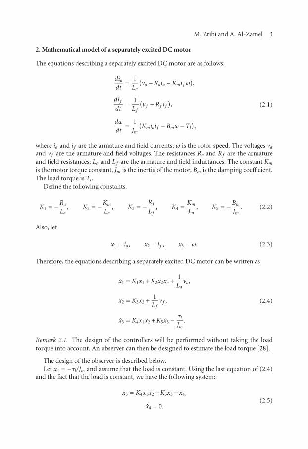
2. Mathematical model of a separately excited DC motor

The equations describing a separately excited DC motor are as follows:

diadt= 1

La

(va−Raia−Kmi f ω

),

di fdt= 1

L f

(v f −Rf i f

),

dω

dt= 1

Jm

(Kmiai f −Bmω−Tl

),

(2.1)

where ia and i f are the armature and field currents; ω is the rotor speed. The voltages vaand v f are the armature and field voltages. The resistances Ra and Rf are the armatureand field resistances; La and L f are the armature and field inductances. The constant Km

is the motor torque constant, Jm is the inertia of the motor, Bm is the damping coefficient.The load torque is Tl.

Define the following constants:

K1 =−Ra

La, K2 =−Km

La, K3 =−

Rf

L f, K4 = Km

Jm, K5 =−Bm

Jm. (2.2)

Also, let

x1 = ia, x2 = i f , x3 = ω. (2.3)

Therefore, the equations describing a separately excited DC motor can be written as

x1 = K1x1 +K2x2x3 +1La

va,

x2 = K3x2 +1L f

v f ,

x3 = K4x1x2 +K5x3− τlJm

.

(2.4)

Remark 2.1. The design of the controllers will be performed without taking the loadtorque into account. An observer can then be designed to estimate the load torque [28].

The design of the observer is described below.Let x4 =−τl/Jm and assume that the load is constant. Using the last equation of (2.4)

and the fact that the load is constant, we have the following system:

x3 = K4x1x2 +K5x3 + x4,

x4 = 0.(2.5)


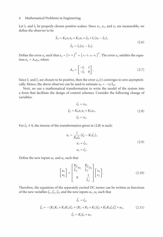
Let l1 and l2 be properly chosen positive scalars. Since x1, x2, and x3 are measurable, wedefine the observer to be

˙x3 = K4x1x2 +K5x3 + x4 + l1(x3− x3

),

˙x4 = l2(x3− x3

).

(2.6)

Define the error eo such that eo =[e3 e4

]T = [ x3−x3 x4−x4

]T. The error eo satisfies the equa-

tion eo = Aoeo, where

Ao =[−l1 1−l2 0

]

. (2.7)

Since l1 and l2 are chosen to be positive, then the error eo(t) converges to zero asymptoti-cally. Hence, the above observer can be used to estimate x4 =−τl/Jm.

Next, we use a mathematical transformation to write the model of the system intoa form that facilitate the design of control schemes. Consider the following change ofvariables:

ζ1 = x3,

ζ2 = K4x1x2 +K5x3,

ζ3 = x2.

(2.8)

For ζ3 �= 0, the inverse of the transformation given in (2.8) is such:

x1 = 1K4ζ3

(ζ2−K5ζ1

),

x2 = ζ3,

x3 = ζ1.

(2.9)

Define the new inputs u1 and u2 such that

[u1

u2

]

=

⎡

⎢⎢⎢⎢⎣

K4

Lax2

K4

L fx1

01L f

⎤

⎥⎥⎥⎥⎦

[vav f

]

. (2.10)

Therefore, the equations of the separately excited DC motor can be written as functionsof the new variables ζ1, ζ2, ζ3, and the new inputs u1, u2 such that

ζ1 = ζ2,

ζ2 =−(K1K5 +K3K5

)ζ1 +

(K1 +K3 +K5

)ζ2 +K2K4ζ1ζ

23 +u1,

ζ3 = K3ζ3 +u2.

(2.11)


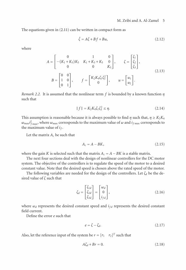
The equations given in (2.11) can be written in compact form as

ζ =Aζ +B f +Bu, (2.12)

where

A=⎡

⎢⎣

0 1 0−(K1 +K3

)K5 K1 +K3 +K5 0

0 0 K3

⎤

⎥⎦ , ζ =

⎡

⎢⎣

ζ1

ζ2

ζ3

⎤

⎥⎦ ,

B =⎡

⎢⎣

0 01 00 1

⎤

⎥⎦ , f =

[K2K4ζ1ζ

23

0

]

, u=[u1

u2

]

.

(2.13)

Remark 2.2. It is assumed that the nonlinear term f is bounded by a known function ηsuch that

‖ f ‖ = K2K4ζ1ζ23 ≤ η. (2.14)

This assumption is reasonable because it is always possible to find η such that, η ≥ K2K4

ωmaxi2f max, where ωmax corresponds to the maximum value of ω and i f max corresponds to

the maximum value of i f .

Let the matrix Ac be such that

Ac =A−BK , (2.15)

where the gain K is selected such that the matrix Ac =A−BK is a stable matrix.The next four sections deal with the design of nonlinear controllers for the DC motor

system. The objective of the controllers is to regulate the speed of the motor to a desiredconstant value. Note that the desired speed is chosen above the rated speed of the motor.

The following variables are needed for the design of the controllers. Let ζd be the de-sired value of ζ such that

ζd =⎡

⎢⎣

ζ1d

ζ2d

ζ3d

⎤

⎥⎦=

⎡

⎢⎣

ωd

0i f d

⎤

⎥⎦ , (2.16)

where ωd represents the desired constant speed and i f d represents the desired constantfield current.

Define the error e such that

e = ζ − ζd. (2.17)

Also, let the reference input of the system be r = [r1 r2]T such that

Aζd +Br = 0. (2.18)


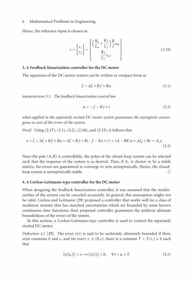
Hence, the reference input is chosen as

r =[r1

r2

]

=

⎡

⎢⎢⎢⎢⎣

(Ra

La+Rf

L f

)B

Jωd

R f

L fi f d

⎤

⎥⎥⎥⎥⎦. (2.19)

3. A Feedback linearization controller for the DC motor

The equations of the DC motor system can be written in compact form as

ζ = Aζ +B f +Bu. (3.1)

proposition 3.1. The feedback linearization control law

u=− f −Ke+ r (3.2)

when applied to the separately excited DC motor system guarantees the asymptotic conver-gence to zero of the errors of the system.

Proof. Using (2.17), (3.1), (3.2), (2.18), and (2.15), it follows that

e = ζ = Aζ +B f +Bu= Aζ +B f +B(− f −Ke+ r)= (A−BK)e+Aζd +Br = Ace.(3.3)

Since the pair (A,B) is controllable, the poles of the closed-loop system can be selectedsuch that the response of the system is as desired. Thus, if Ac is chosen to be a stablematrix, the errors are guaranteed to converge to zero asymptotically. Hence, the closed-loop system is asymptotically stable. �

4. A Corless-Leitmann-type controller for the DC motor

When designing the feedback linearization controller, it was assumed that the nonlin-earities of the system can be canceled accurately. In general, this assumption might notbe valid. Corless and Leitmann [29] proposed a controller that works well for a class ofnonlinear systems that has matched uncertainties which are bounded by some knowncontinuous time functions; their proposed controller guarantees the uniform ultimateboundedness of the errors of the system.

In this section, a Corless-Leitmann-type controller is used to control the separatelyexcited DC motor.

Definition 4.1 [29]. The error e(t) is said to be uniformly ultimately bounded if thereexist constants b and c, and for every rc ∈ (0,c), there is a constant T = T(rc) ≥ 0 suchthat

∥∥e(t0)∥∥ < rc=⇒

∥∥e(t)

∥∥ < b, ∀t > t0 +T. (4.1)


The proposed control law is divided into a linear part and a nonlinear part. The linearpart of the controller is designed using the pole placement technique. The nonlinear partof the controller is designed to resemble a Corless-Leitmann-type controller.

Let the symmetric positive definite matrix P1 be the solution of the following Lya-punov equation:

ATc P1 +P1Ac =−Q1 (4.2)

with Q1 =QT1 > 0.

proposition 4.2. The control law given by (4.3)–(4.6) when applied to the separately ex-cited DC motor guarantees the uniform ultimate boundedness of the errors of the system:

u= uL +uN (4.3)

with

uL =−Ke+ r, (4.4)

uN =

⎧⎪⎪⎪⎨

⎪⎪⎪⎩

− μ1∥∥μ1∥∥η if

∥∥μ1∥∥ > ε,

−μ1

εη if

∥∥μ1∥∥≤ ε,

(4.5)

with

μ1 = ηBTP1e (4.6)

and η > 0, and ε is a small positive scalar.

Proof. Using (2.17), (3.1), (4.3), (4.4), (2.15) and (2.18), it follows that

e = Aζ +B f +Bu= Aζ +B f +B(−Ke+ r +uN

)= Ace+B f +BuN. (4.7)

Consider the following Lyapunov function candidate:

V1 = eTP1e. (4.8)

Note that V1 > 0 for e �= 0 and V1 = 0 for e = 0. Taking the derivative of V1 with respectto time and using (4.7) and (4.2), it follows that

V1 = eTP1e+ eTP1e

= (Ace+B f +BuN)TP1e+ eTP1

(Ace+B f +BuN

)

=−eTQe+ 2eTP1BuN + 2 f TBTP1e.

(4.9)

We will treat the two cases ‖μ1‖ > ε and ‖μ1‖ ≤ ε separately.


For the case when ‖μ1‖ > ε and uN =−(μ1/‖μ1‖)η, (4.9) implies that

V1 =−eTQe+ 2eTP1BuN + 2 f TBTP1e

=−eTQ1e− 2eTP1Bμ1∥∥μ1∥∥η+ 2 f TBTP1e

≤−eTQ1e− 2∥∥BTP1e

∥∥η+ 2‖ f ‖T∥∥BTP1e

∥∥

≤−eTQ1e.

(4.10)

For the case when ‖μ1‖ ≤ ε and uN =−(μ1/ε)η, (4.9) implies that

V1 =−eTQ1e+ 2eTP1BuN + 2 f TBTP1e

=−eTQ1e− 2eTP1Bμ1

εη+ 2 f TBTP1e

≤−eTQ1e− 2

∥∥BTP1e

∥∥2

εη2 + 2‖ f ‖T∥∥BTP1e

∥∥

≤−eTQ1e+ 2∥∥BTP1e

∥∥η2

≤−eTQ1e+ 2ε.

(4.11)

Therefore, it can be concluded that in both cases,

V1 ≤−λmin(Q1)‖e‖2 + 2ε, (4.12)

where λmin(Q1) is the minimum eignevalue of Q1. Using (4.8) and (4.12), it can be con-cluded that V1 decreases monotonically along any trajectory of the closed-loop systemuntil it reaches the compact set:

Λs ={e |V1 ≤Vs

}, (4.13)

where Vs can be easily determined from (4.8) and (4.12).Therefore, it can be concluded that the errors are uniformly ultimately bounded.

Hence the control scheme (4.3)–(4.6) guarantees the uniform ultimate boundedness ofthe errors of the motor system.

The discontinuous nature of the Corless-Leitmann-type controller may be harmful tothe motor. Hence, two continuous nonlinear state-feedback controllers are designed next.The controllers are similar to the Corless-Leitmann-type controller in that they workwell for a class of nonlinear uncertain systems that has matched uncertainties which arebounded by some known continuous time functions. However, the main advantage ofthese control schemes are that they are continuous in nature. �


5. Continuous nonlinear controllers for the DC motor

5.1. First continuous nonlinear controller for the DC motor. The control scheme is di-vided into a linear part and a nonlinear part. The linear control part is designed usingthe pole placement technique. The continuous nonlinear part of the controller is moti-vated by the work of [30]. The proposed controller has the advantage of guaranteeing theexponential stability of the closed-loop system.

Let the symmetric positive definite matrix P2 be the solution of the following algebraicRiccati equation:

ATc P2 +P2Ac− 2P2BB

TP2 =−Q2, (5.1)

where Q2 =QT2 > 0.

Define

μ2 = ηBTP2e, η > 0, (5.2)

also let ε and β be small positive scalars.

proposition 5.1. The control law given by (5.3)–(5.6) when applied to the separately ex-cited DC motor guarantees the exponential convergence to zero of the errors of the system:

u= uL +uN (5.3)

with

uL =−Ke+ r, (5.4)

uN =−BTP2e−φc, (5.5)

φc = μ2∥∥μ2∥∥2

∥∥μ2∥∥3

+ ε3 exp(−3βt)η. (5.6)

Proof. Consider the following Lyapunov function candidate:

V2 = eTP2e. (5.7)

Note that V2 > 0 for e �= 0 and V2 = 0 for e = 0. Equation (5.7) implies that λ1‖e‖2 ≤V2 ≤λ2‖e‖2, where λ1 is the minimum eigenvalue of P2 and λ2 is the maximum eigenvalue ofP2.

Using (2.17), (3.1), (4.3), (4.4), (2.15), (2.18), and (5.5), it follows that

eTP2e =(Ace+B f +BuN

)TP2e =

(eTAT

c + f TBT − eTP2BBT −φT

c BT)P2e. (5.8)


Taking the derivative of V2 with respect to time and using (5.8) and (5.3)–(5.6), it followsthat

V2 = eTP2e+ eTP2e

= (eTATc + f TBT − eTP2BB

T −φTc B

T)P2e+ eTP2

(Ace+B f −BBTP2e−Bφc

)

=−eTQ2e+ 2eTP2B f − 2eTP2BφTc

=−eTQ2e+ 2eTP2B f − 2eTP2Bμ2∥∥μ2∥∥2

∥∥μ2∥∥3

+ ε3 exp(−3βt)η

≤−eTQ2e− 2∥∥BTP2eη

∥∥4

∥∥BTP2eη

∥∥3

+ ε3 exp(−3βt)η+ 2

∥∥BTP2eη

∥∥

≤−eTQ2e+2∥∥BTP2eη

∥∥ε3 exp(−3βt)

∥∥BTP2eη

∥∥3

+ ε3 exp(−3βt)η

≤−eTQ2e+ 2εexp(−βt)

≤−λ3‖e‖2 + 2εexp(−βt).

(5.9)

In the above, we used the fact that

0≤ ab3

a3 + b3≤ b, ∀a,b ≥ 0, a3 + b3 �= 0. (5.10)

and λ3 is the minimum eigenvalue of Q2.Let κ= λ3/λ2, it follows that

V2 ≤−κV2 + 2εexp(−βt). (5.11)

Thus, it can be concluded that the error e(t) is globally exponentially stable. Moreover,the convergence rate of the errors is such:

∥∥e(t)

∥∥≤

⎧⎪⎪⎪⎪⎪⎪⎨

⎪⎪⎪⎪⎪⎪⎩

[λ2

λ1

∥∥e(0)

∥∥2

exp(−κt) +2ελ1t exp(−κt)

]1/2

if β = κ,

[λ2

λ1

∥∥e(0)

∥∥2

exp(−κt) +2ε

λ1(κ−β)

(exp(−βt)− exp(−κt))

]1/2

if β �= κ.

(5.12)

Hence, it can be concluded that the proposed control scheme (5.3)–(5.6) when appliedto the DC motor system guarantees the exponential convergence to zero of the errors ofthe system. �


5.2. Second continuous nonlinear controller for the DC motor. Again, the controlscheme is divided into a linear part and a nonlinear part. The linear controller part isdesigned using the pole placement technique. The continuous nonlinear part of the con-troller is motivated by the work of [31].

Let the symmetric positive definite matrix P3 be the solution of the Lyapunov equa-tion:

ATc P3 +P3Ac =−Q3 (5.13)

with Q3 =QT3 > 0.

proposition 5.2. The control law

u= uL +uN (5.14)

with

uL =−Ke+ r, uN =−γoBTP3e (5.15)

when applied to the separately excited DC motor guarantees the exponential convergence ofthe errors of the system such that

∥∥e(t)

∥∥≤ co exp

(− ν(t− to

))+μ, (5.16)

where

co =√√√√λmax

(P3)

λmin(P3)∥∥e(to)∥∥, ν= λmin

(Q3)

2λmax(P3) , μ= η

√√√√ λmax

(P3)

γoλmin(P3)λmin

(Q3) ,

(5.17)

and λmax(•) is the maximum eigenvalue of •, and λmin(•) is the minimum eigenvalue of •.

Proof. Consider the following Lyapunov function candidate:

V3 = eTP3e. (5.18)

Note that V3 > 0 for e �= 0 and V3 = 0 for e = 0.Taking the derivative of V3 with respect to time and using (2.17), (3.1), (2.15), and

(5.11)–(5.14), it follows that

V3 = eTP3e+ eTP3e

= (Ace+B f +BuN)TP3e+ eTP3

(Ace+B f +BuN

)

=−eTQ3e+ 2eTP3BuN + 2 f TBTP3e

=−eTQ3e+ 2eTP3B(− γoB

TP3e)

+ 2 f TBTP3e

≤−eTQ3e− 2γo∥∥BTP3e

∥∥2

+ 2∥∥BTP3e

∥∥η


Reference

DSP controller card

Controller PWMPower

moduleDC motor

system

Current sensor

Tacho-generator

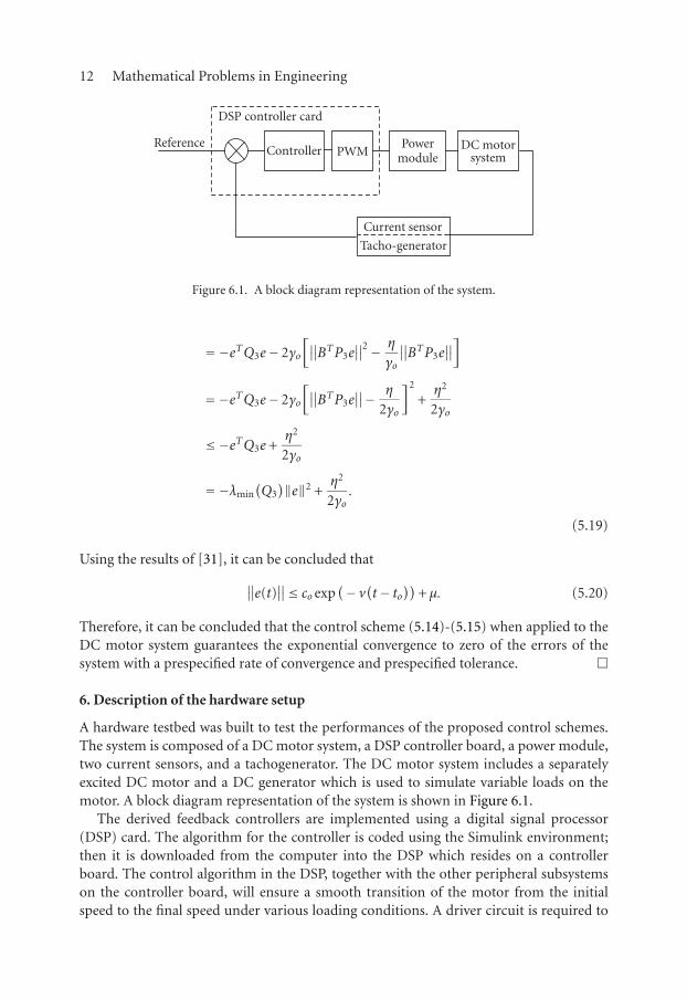
Figure 6.1. A block diagram representation of the system.

=−eTQ3e− 2γo

[∥∥BTP3e

∥∥2− η

γo

∥∥BTP3e

∥∥]

=−eTQ3e− 2γo

[∥∥BTP3e

∥∥− η

2γo

]2

+η2

2γo

≤−eTQ3e+η2

2γo

=−λmin(Q3)‖e‖2 +

η2

2γo.

(5.19)

Using the results of [31], it can be concluded that

∥∥e(t)

∥∥≤ co exp

(− v(t− to

))+μ. (5.20)

Therefore, it can be concluded that the control scheme (5.14)-(5.15) when applied to theDC motor system guarantees the exponential convergence to zero of the errors of thesystem with a prespecified rate of convergence and prespecified tolerance. �

6. Description of the hardware setup

A hardware testbed was built to test the performances of the proposed control schemes.The system is composed of a DC motor system, a DSP controller board, a power module,two current sensors, and a tachogenerator. The DC motor system includes a separatelyexcited DC motor and a DC generator which is used to simulate variable loads on themotor. A block diagram representation of the system is shown in Figure 6.1.

The derived feedback controllers are implemented using a digital signal processor(DSP) card. The algorithm for the controller is coded using the Simulink environment;then it is downloaded from the computer into the DSP which resides on a controllerboard. The control algorithm in the DSP, together with the other peripheral subsystemson the controller board, will ensure a smooth transition of the motor from the initialspeed to the final speed under various loading conditions. A driver circuit is required to


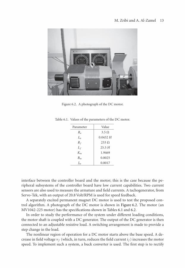
Figure 6.2. A photograph of the DC motor.

Table 6.1. Values of the parameters of the DC motor.

Parameter Value

Ra 3.5 Ω

La 0.0432 H

Rf 233 Ω

Lf 25.5 H

Km 1.9469

Bm 0.0025

Jm 0.0017

interface between the controller board and the motor; this is the case because the pe-ripheral subsystems of the controller board have low current capabilities. Two currentsensors are also used to measure the armature and field currents. A tachogenerator, fromServo-Tek, with an output of 20.8 Volt/RPM is used for speed feedback.

A separately excited permanent magnet DC motor is used to test the proposed con-trol algorithm. A photograph of the DC motor is shown in Figure 6.2. The motor (anMV1042-225 motor) has the specifications shown in Tables 6.1 and 6.2.

In order to study the performance of the system under different loading conditions,the motor shaft is coupled with a DC generator. The output of the DC generator is thenconnected to an adjustable resistive load. A switching arrangement is made to provide astep change in the load.

The nonlinear region of operation for a DC motor starts above the base speed. A de-crease in field voltage v f (which, in turn, reduces the field current i f ) increases the motorspeed. To implement such a system, a buck converter is used. The first step is to rectify


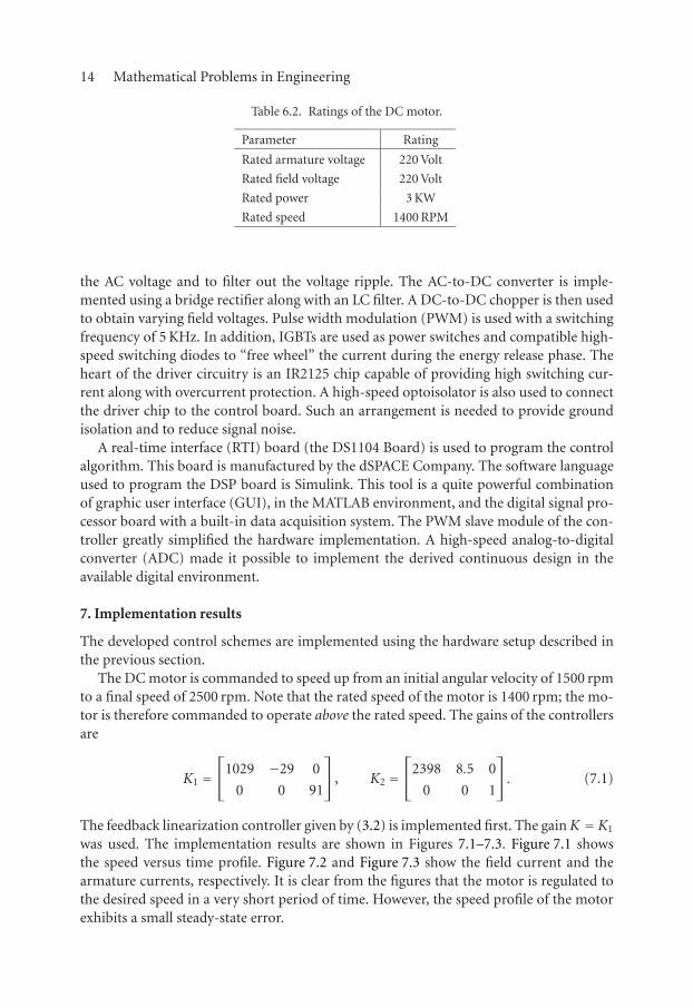
Table 6.2. Ratings of the DC motor.

Parameter Rating

Rated armature voltage 220 Volt

Rated field voltage 220 Volt

Rated power 3 KW

Rated speed 1400 RPM

the AC voltage and to filter out the voltage ripple. The AC-to-DC converter is imple-mented using a bridge rectifier along with an LC filter. A DC-to-DC chopper is then usedto obtain varying field voltages. Pulse width modulation (PWM) is used with a switchingfrequency of 5 KHz. In addition, IGBTs are used as power switches and compatible high-speed switching diodes to “free wheel” the current during the energy release phase. Theheart of the driver circuitry is an IR2125 chip capable of providing high switching cur-rent along with overcurrent protection. A high-speed optoisolator is also used to connectthe driver chip to the control board. Such an arrangement is needed to provide groundisolation and to reduce signal noise.

A real-time interface (RTI) board (the DS1104 Board) is used to program the controlalgorithm. This board is manufactured by the dSPACE Company. The software languageused to program the DSP board is Simulink. This tool is a quite powerful combinationof graphic user interface (GUI), in the MATLAB environment, and the digital signal pro-cessor board with a built-in data acquisition system. The PWM slave module of the con-troller greatly simplified the hardware implementation. A high-speed analog-to-digitalconverter (ADC) made it possible to implement the derived continuous design in theavailable digital environment.

7. Implementation results

The developed control schemes are implemented using the hardware setup described inthe previous section.

The DC motor is commanded to speed up from an initial angular velocity of 1500 rpmto a final speed of 2500 rpm. Note that the rated speed of the motor is 1400 rpm; the mo-tor is therefore commanded to operate above the rated speed. The gains of the controllersare

K1 =⎡

⎣1029 −29 0

0 0 91

⎤

⎦ , K2 =⎡

⎣2398 8.5 0

0 0 1

⎤

⎦ . (7.1)

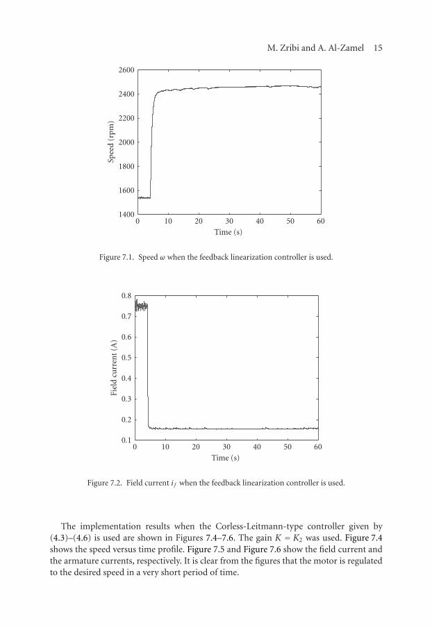
The feedback linearization controller given by (3.2) is implemented first. The gain K = K1

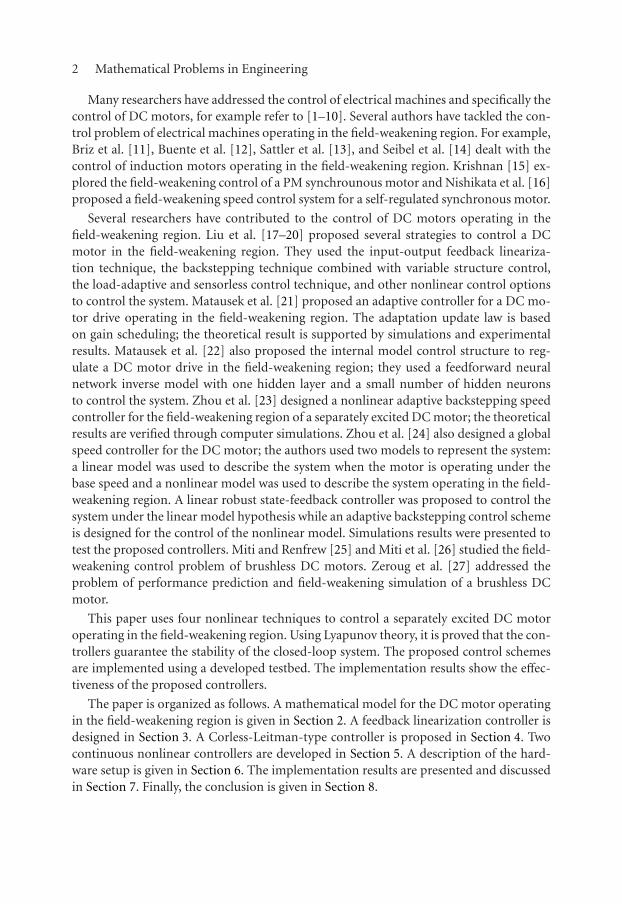
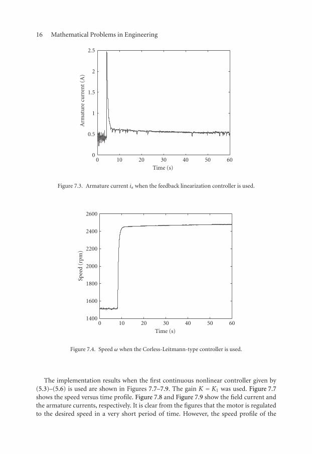
was used. The implementation results are shown in Figures 7.1–7.3. Figure 7.1 showsthe speed versus time profile. Figure 7.2 and Figure 7.3 show the field current and thearmature currents, respectively. It is clear from the figures that the motor is regulated tothe desired speed in a very short period of time. However, the speed profile of the motorexhibits a small steady-state error.


6050403020100

Time (s)

1400

1600

1800

2000

2200

2400

2600

Spee

d(r

pm)

Figure 7.1. Speed ω when the feedback linearization controller is used.

6050403020100

Time (s)

0.1

0.2

0.3

0.4

0.5

0.6

0.7

0.8

Fiel

dcu

rren

t(A

)

Figure 7.2. Field current i f when the feedback linearization controller is used.

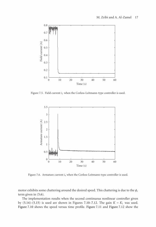
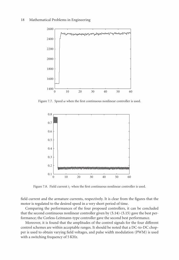
The implementation results when the Corless-Leitmann-type controller given by(4.3)–(4.6) is used are shown in Figures 7.4–7.6. The gain K = K2 was used. Figure 7.4shows the speed versus time profile. Figure 7.5 and Figure 7.6 show the field current andthe armature currents, respectively. It is clear from the figures that the motor is regulatedto the desired speed in a very short period of time.


6050403020100

Time (s)

0

0.5

1

1.5

2

2.5

Arm

atu

recu

rren

t(A

)

Figure 7.3. Armature current ia when the feedback linearization controller is used.

6050403020100

Time (s)

1400

1600

1800

2000

2200

2400

2600

Spee

d(r

pm)

Figure 7.4. Speed ω when the Corless-Leitmann-type controller is used.

The implementation results when the first continuous nonlinear controller given by(5.3)–(5.6) is used are shown in Figures 7.7–7.9. The gain K = K1 was used. Figure 7.7shows the speed versus time profile. Figure 7.8 and Figure 7.9 show the field current andthe armature currents, respectively. It is clear from the figures that the motor is regulatedto the desired speed in a very short period of time. However, the speed profile of the


6050403020100

Time (s)

0.1

0.2

0.3

0.4

0.5

0.6

0.7

0.8

Fiel

dcu

rren

t(A

)

Figure 7.5. Field current i f when the Corless-Leitmann-type controller is used.

6050403020100

Time (s)

0

0.5

1

1.5

2

2.5

3

3.5

Arm

atu

recu

rren

t(A

)

Figure 7.6. Armature current ia when the Corless-Leitmann-type controller is used.

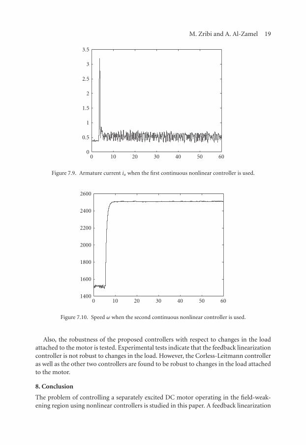
motor exhibits some chattering around the desired speed. This chattering is due to the φcterm given in (5.6).

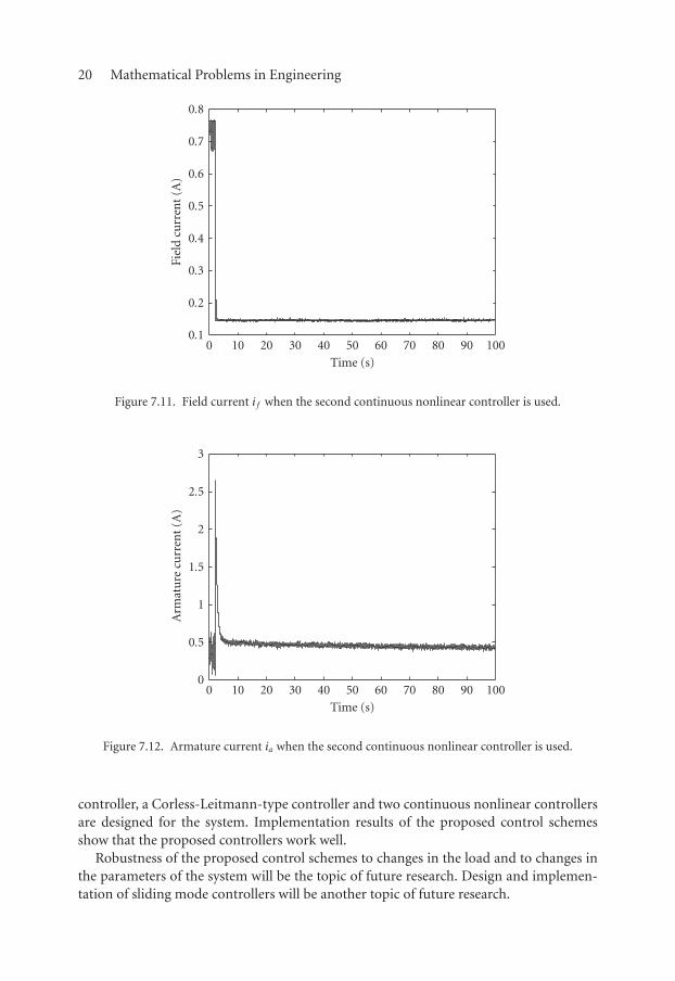
The implementation results when the second continuous nonlinear controller givenby (5.14)-(5.15) is used are shown in Figures 7.10–7.12. The gain K = K1 was used.Figure 7.10 shows the speed versus time profile. Figure 7.11 and Figure 7.12 show the


60504030201001400

1600

1800

2000

2200

2400

2600

Figure 7.7. Speed ω when the first continuous nonlinear controller is used.

60504030201000.1

0.2

0.3

0.4

0.5

0.6

0.7

0.8

Figure 7.8. Field current i f when the first continuous nonlinear controller is used.

field current and the armature currents, respectively. It is clear from the figures that themotor is regulated to the desired speed in a very short period of time.

Comparing the performances of the four proposed controllers, it can be concludedthat the second continuous nonlinear controller given by (5.14)-(5.15) gave the best per-formance; the Corless-Leitmann-type controller gave the second best performance.

Moreover, it is found that the amplitudes of the control signals for the four differentcontrol schemes are within acceptable ranges. It should be noted that a DC-to-DC chop-per is used to obtain varying field voltages, and pulse width modulation (PWM) is usedwith a switching frequency of 5 KHz.


60504030201000

0.5

1

1.5

2

2.5

3

3.5

Figure 7.9. Armature current ia when the first continuous nonlinear controller is used.

60504030201001400

1600

1800

2000

2200

2400

2600

Figure 7.10. Speed ω when the second continuous nonlinear controller is used.

Also, the robustness of the proposed controllers with respect to changes in the loadattached to the motor is tested. Experimental tests indicate that the feedback linearizationcontroller is not robust to changes in the load. However, the Corless-Leitmann controlleras well as the other two controllers are found to be robust to changes in the load attachedto the motor.

8. Conclusion

The problem of controlling a separately excited DC motor operating in the field-weak-ening region using nonlinear controllers is studied in this paper. A feedback linearization


1009080706050403020100

Time (s)

0.1

0.2

0.3

0.4

0.5

0.6

0.7

0.8

Fiel

dcu

rren

t(A

)

Figure 7.11. Field current i f when the second continuous nonlinear controller is used.

1009080706050403020100

Time (s)

0

0.5

1

1.5

2

2.5

3

Arm

atu

recu

rren

t(A

)

Figure 7.12. Armature current ia when the second continuous nonlinear controller is used.

controller, a Corless-Leitmann-type controller and two continuous nonlinear controllersare designed for the system. Implementation results of the proposed control schemesshow that the proposed controllers work well.

Robustness of the proposed control schemes to changes in the load and to changes inthe parameters of the system will be the topic of future research. Design and implemen-tation of sliding mode controllers will be another topic of future research.


Acknowledgment

This research was supported by Kuwait University under research Grant no. EE 05/02.

References

[1] M. Bodson and J. Chiasson, “Differential-geometric methods for control of electric motors,”International Journal of Robust and Nonlinear Control, vol. 8, no. 11, pp. 923–954, 1998.

[2] M. Bodson, J. Chiasson, and R. Novotnak, “High-performance induction motor control viainput-output linearization,” IEEE Control Systems Magazine, vol. 14, no. 4, pp. 25–33, 1994.

[3] T. C. Burg, D. M. Dawson, J. Hu, and P. Vedagarbha, “Velocity tracking control for a separatelyexcited DC motor without velocity measurements,” in Proceedings of the American Control Con-ference, vol. 1, pp. 1051–1056, Baltimore, Md, USA, June-July 1994.

[4] J. Chiasson, “Nonlinear differential-geometric techniques for control of a series DC motor,”IEEE Transactions on Control Systems Technology, vol. 2, no. 1, pp. 35–42, 1994.

[5] J. Chiasson and M. Bodson, “Nonlinear control of a shunt DC motor,” IEEE Transactions onAutomatic Control, vol. 38, no. 11, pp. 1662–1666, 1993.

[6] R. Harmsen and J. Jiang, “Control of a separately excited DC motor using on-line linearization,”in Proceedings of the American Control Conference, vol. 2, pp. 1879–1883, Baltimore, Md, USA,June-July 1994.

[7] M. H. Nehrir and F. Fatehi, “Tracking control of DC motors via input-output linearization,”Electric Machines and Power Systems, vol. 24, no. 3, pp. 237–247, 1996.

[8] P. D. Olivier, “Feedback linearization of DC motors,” IEEE Transactions on Industrial Electronics,vol. 38, no. 6, pp. 498–501, 1991.

[9] D. G. Taylor, “Nonlinear control of electric machines: an overview,” IEEE Control Systems Mag-azine, vol. 14, no. 6, pp. 41–51, 1994.

[10] V. I. Utkin, “Sliding mode control design principles and applications to electric drives,” IEEETransactions on Industrial Electronics, vol. 40, no. 1, pp. 23–36, 1993.

[11] F. Briz, A. Diez, M. W. Degner, and R. D. Lorenz, “Current and flux regulation in field-weakeningoperation [of induction motors] ,” IEEE Transactions on Industry Applications, vol. 37, no. 1, pp.42–50, 2001.

[12] A. Buente, H. Grotstollen, and P. Krafka, “Field weakening of induction motors in a very wideregion with regard to parameter uncertainties,” in Proceedings of the 27th Annual IEEE PowerElectronics Specialists Conference (PESC ’96), vol. 1, pp. 944–950, Maggiore, Italy, January 1996.

[13] K. Sattler, U. Schaefer, and R. Gheysens, “Field oriented control of an induction motor withfield weakening under consideration of saturation and rotor heating,” in Proceedings of the 4thInternational Conference on Power Electronics and Variable-Speed Drives, pp. 286–291, London,UK, July 1990.

[14] B. J. Seibel, T. M. Rowan, and R. J. Kerkman, “Field-oriented control of an induction machinein the field-weakening region with DC-link and load disturbance rejection,” IEEE Transactionson Industry Applications, vol. 33, no. 6, pp. 1578–1584, 1997.

[15] R. Krishnan, “Control and operation of PM synchronous motor drives in the field-weakeningregion,” in Proceedings of the 19th International Conference on Industrial Electronics, Control andInstrumentation (IECON ’93), vol. 2, pp. 745–750, Maui, Hawaii, USA, November 1993.

[16] S. Nishikata, W. Takanami, T. Kataoka, and A. Ishizaki, “Consideration to the operation limit of afield-weakening speed control system for a self-controlled synchronous motor,” in Proceedings ofthe 5th European Conference on Power Electronics and Applications, vol. 5, pp. 354–359, Brighton,UK, September 1993.

[17] Z. Z. Liu and F. L. Luo, “Nonlinear multi-input multi-output control of DC motor in fieldweak-ening region,” in Proceedings of International Conference Electric Machines and Drives (IEMD’99), pp. 688–690, Seattle, Wash, USA, May 1999.


[18] Z. Z. Liu, F. L. Luo, and M. H. Rashid, “Nonlinear load-adaptive MIMO controller for highperformance DC motor field weakening,” in IEEE Power Engineering Society Winter Meeting,vol. 1, pp. 332–337, Singapore, January 2000.

[19] Z. Z. Liu, F. L. Luo, and M. H. Rashid, “Speed nonlinear control of DC motor drive with fieldweakening,” IEEE Transactions on Industry Applications, vol. 39, no. 2, pp. 417–423, 2003.

[20] F. L. Luo, Z. Z. Liu, and D. Tien, “Nonlinear field weakening controller of a separately excited DCmotor,” in Proceedings of the International Conference on Energy Management and Power Delivery(EMPD ’98), vol. 2, pp. 552–557, Singapore, March 1998.

[21] M. R. Matausek, B. I. Jeftenic, D. M. Miljkovic, and M. Z. Bebic, “Gain scheduling control of DCmotor drive with field weakening,” IEEE Transactions on Industrial Electronics, vol. 43, no. 1, pp.153–162, 1996.

[22] M. R. Matausek, D. M. Miljkovic, and B. I. Jeftenic, “Nonlinear multi-input-multi-output neu-ral network control of DC motor drive with field weakening,” IEEE Transactions on IndustrialElectronics, vol. 45, no. 1, pp. 185–187, 1998.

[23] J. Zhou, Y. Wang, and R. Zhou, “Adaptive backstepping control of separately excited DC mo-tor with uncertainties,” in Proceedings of International Conference on Power System Technology(PowerCon ’00), vol. 1, pp. 91–96, Perth, Western Australia, August 2000.

[24] J. Zhou, Y. Wang, and R. Zhou, “Global speed control of separately excited DC motor,” in Pro-ceedings of the IEEE Power Engineering Society Winter Meeting, vol. 3, pp. 1425–1430, Columbus,Ohio, USA, January-February 2001.

[25] G. K. Miti and A. C. Renfrew, “Analysis, simulation and microprocessor implementation of acurrent profiling scheme for field-weakening applications and torque ripple control in brushlessDC motors,” in Proceedings of the 9th International Conference on Electrical Machines and Drives(EMD ’99), pp. 361–365, Canterbury, UK, September 1999.

[26] G. K. Miti, A. C. Renfrew, and B. J. Chalmers, “Field-weakening regime for brushless DC motorsbased on instantaneous power theory,” IEE Proceedings: Electric Power Applications, vol. 148,no. 3, pp. 265–271, 2001.

[27] H. Zeroug, D. Holliday, D. Grant, and N. Dahnoun, “Performance prediction and field weaken-ing simulation of a brushless DC motor,” in Proceedings of the 8th International Conference onPower Electronics and Variable Speed Drives, pp. 321–326, London, UK, September 2000.

[28] M. Zribi and J. Chiasson, “Position control of a PM stepper motor by exact linearization,” IEEETransactions on Automatic Control, vol. 36, no. 5, pp. 620–625, 1991.

[29] M. J. Corless and G. Leitmann, “Continuous state feedback guaranteeing uniform ultimateboundedness for uncertain dynamic systems,” IEEE Transactions on Automatic Control, vol. 26,no. 5, pp. 1139–1144, 1981.

[30] S. K. Nguang and M. Fu, “Global quadratic stabilization of a class of nonlinear systems,” Inter-national Journal of Robust and Nonlinear Control, vol. 8, no. 6, pp. 483–497, 1998.

[31] S. Zenieh and M. Corless, “Simple robust r-α tracking controllers for uncertain fully-actuatedmechanical systems,” Transactions of the ASME, Journal of Dynamic Systems, Measurement andControl, vol. 119, no. 4, pp. 821–825, 1997.

Mohamed Zribi: Department of Electrical Engineering, Kuwait University, P.O. Box 5969,Safat 13060, KuwaitEmail address: [email protected]

Adel Al-Zamel: Department of Electrical Engineering, Kuwait University, P.O. Box 5969,Safat 13060, KuwaitEmail address: [email protected]

mailto:[email protected]

mailto:[email protected]

Documents

Field-Weakening Nonlinear Control of a Separately Excited ...€¦ · a separately excited DC motor operating in the ﬁeld-weakening region. A feedback lin-earization controller,