Field&Solving &&

Numerical&modeling&of&fields&and&

distribu7ons&

Fields&and&PDEs&

•  A&very&common&problem&which&we&want&to&simulate&is&a&scalar&or&vector&distribu7on&prescribed&by&a&single&or&coupled&set&of&par7al&differen7al&equa7ons&(PDE).&

•  Examples&are:&– Heat&Flow.&–  Poisson&equa7on.&– Maxwell’s&equa7ons.&

–  Schrödinger's&equa7on.&–  Stress/strain&equa7ons.&&– DriM/diffusion&transport.&

Solution of PDE’s using numerical methods

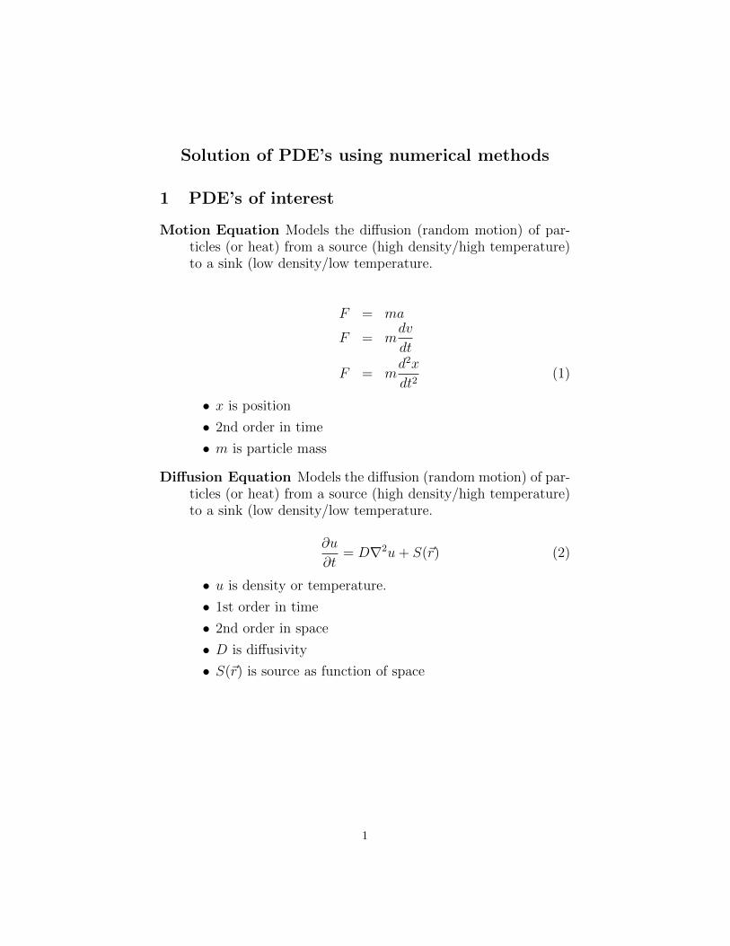
1 PDE’s of interest

Motion Equation Models the di↵usion (random motion) of par-ticles (or heat) from a source (high density/high temperature)to a sink (low density/low temperature.

F = ma

F = m

dv

dt

F = m

d

2x

dt

2(1)

• x is position

• 2nd order in time

• m is particle mass

Di↵usion Equation Models the di↵usion (random motion) of par-ticles (or heat) from a source (high density/high temperature)to a sink (low density/low temperature.

@u

@t

= Dr2u+ S(~r) (2)

• u is density or temperature.

• 1st order in time

• 2nd order in space

• D is di↵usivity

• S(~r) is source as function of space

1

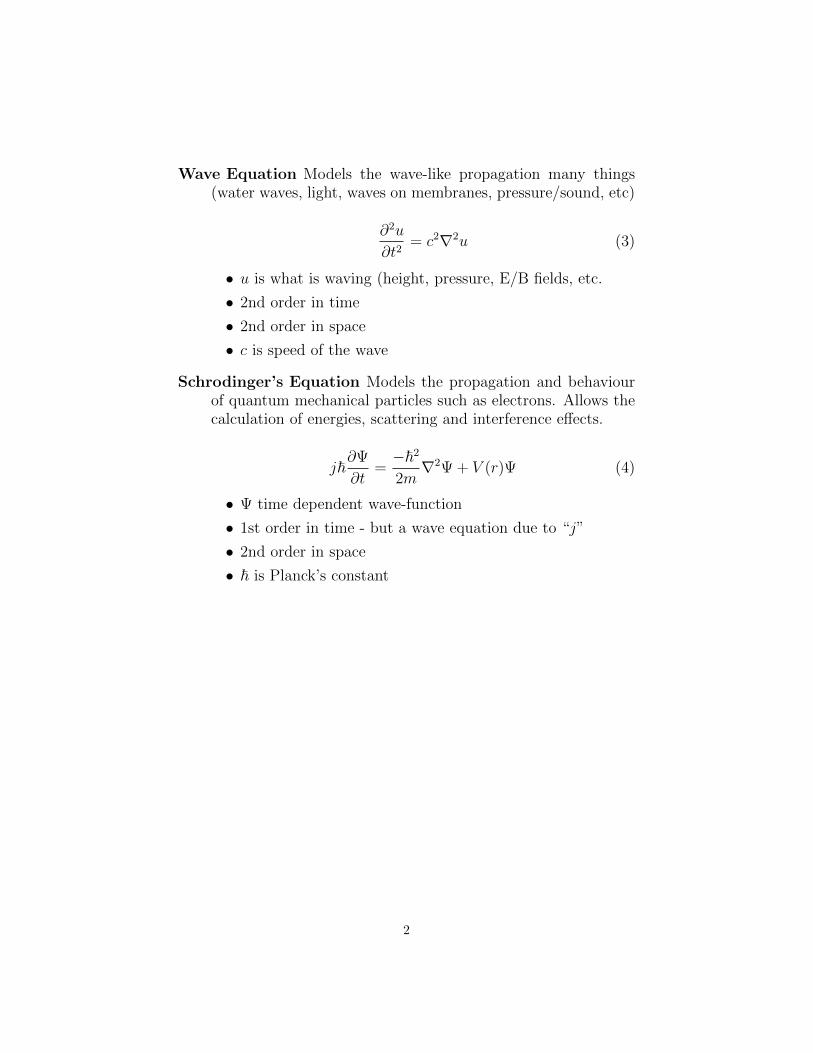
Wave Equation Models the wave-like propagation many things(water waves, light, waves on membranes, pressure/sound, etc)

@

2u

@t

2= c

2r2u (3)

• u is what is waving (height, pressure, E/B fields, etc.

• 2nd order in time

• 2nd order in space

• c is speed of the wave

Schrodinger’s Equation Models the propagation and behaviourof quantum mechanical particles such as electrons. Allows thecalculation of energies, scattering and interference e↵ects.

j~@ @t

=�~22m

r2 + V (r) (4)

• time dependent wave-function

• 1st order in time - but a wave equation due to “j”

• 2nd order in space

• ~ is Planck’s constant

2

2 Analytical Solutions

Solve equations using mathematics and experience.

2.1 Simple case motion equation:

F = m

d

2x

dt

2(5)

Must know the force present. Let’s assume F = at,

d

2x

dt

2=

at

m

(6)

use integration:

dx

dt

=at

2

2m+ A – Integrate once

x(t) =at

3

6m+ At+B – Integrate again (7)

A and B are integration constants and are unknown! How dowe obtain those. This is a time dependent problem known asan initial value problem. We have to known the initial stateof the system,

x(0) = X0

dx

dt

= v(0) = V0 (8)

this gives,

B = X0

A = V0 (9)

3

2.2 Wave equation:

@

2u

@t

2= c

2r2u

@

2u

@t

2= c

2d2u

dx

2(10)

The is a partial di↵erential equation (time and space) morecomplicated. Lets assume:

u(x, t) = U(x)V (t) using separation of variables (11)

@

2u

@t

2= c

2d2u

dx

2

U

@

2V

@t

2= V c

2d2U

dx

2

@

2V

@t

2

1

c

2V

=d

2U

dx

2

1

U

= �� must be a constant! (12)

Lets take the x part U(x),

d

2U

dx

2

1

U

= ��

d

2U

dx

2= ��U

A solution for this is U = A sin(kx) – experience!. We use,

d

2U

dx

2= �Ak

2 sin(kx) (13)

and we have

�Ak

2 sin(kx) = ��A sin(kx) (14)

which implies that � = k

2 and we have a solution.

4

2.3 boundary value problems

However, � and A are still unknown. The equation is only de-pendent on space and we need to know the boundary conditionsto determine these values – the values of U at the boundaries.

This is a particularly interesting problem as the boundariesdetermine the allowable solutions. For example let us say wehave a string fixed at both ends. Then,

U(0) = 0 (15)

U(L) = 0 (16)

where L is the length of the string.

We know that Asin(0) = 0 so that end works.

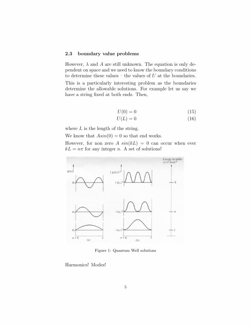
However, for non zero A sin(kL) = 0 can occur when everkL = n⇡ for any integer n. A set of solutions!

Figure 1: Quantum Well solutions

Harmonics! Modes!

5

2.4 Linear and non-linear

The wave equation and the Di↵usion equation are linear equa-tions.

For a linear equation such as the equation if we have two validsolutions to the problem such as:

S1 = sin(k1x) (17)

S2 = sin(k2x) (18)

(19)

then a valid solution will be:

S3 = aS1 + bS2 (20)

where a and b are arbitrary constants. Superposition!

Lots of equations are non-linear equation means that superpo-sition does not work and if A(x) and B(x) are two solutions fora PDE then

C(x) = aA(x) + bB(x) (21)

is not. Reality is non-linear – we make it linear so we can solveit.

2.5 Complexity

This analytical approach works for simple problems, knowndi�cult ones or if you are a very good mathematician.

However, if the problem has complicated geometry, complicatedforcing terms, or is non-linear ie :

@

2u

@t

2= c(x)2

d

2u

dx

2(22)

where c(x) = ↵x

2 + �x+ � and we have:

@

2u

@t

2= (↵x2 + �x+ �)2

d

2u

dx

2(23)

it is very di�cult to solve so we use a numerical approach.

6

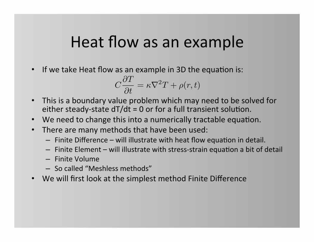
Heat&flow&as&an&example&

•  If&we&take&Heat&flow&as&an&example&in&3D&the&equa7on&is:&

•  This&is&a&boundary&value&problem&which&may&need&to&be&solved&for&either&steady\state&dT/dt&=&0&or&for&a&full&transient&solu7on.&

•  We&need&to&change&this&into&a&numerically&tractable&equa7on.&

•  There&are&many&methods&that&have&been&used:&

–  Finite&Difference&–&will&illustrate&with&heat&flow&equa7on&in&detail.&–  Finite&Element&–&will&illustrate&with&stress\strain&equa7on&a&bit&of&detail&

–  Finite&Volume&

–  So&called&“Meshless&methods”&

•  We&will&first&look&at&the&simplest&method&Finite&Difference&

C@T

@t= r2T + ⇢(r, t)

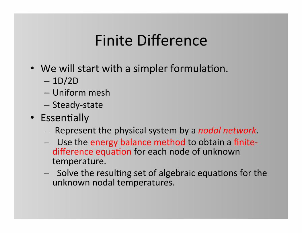
Finite&Difference&

•  We&will&start&with&a&simpler&formula7on. &&–  1D/2D&&– Uniform&mesh&

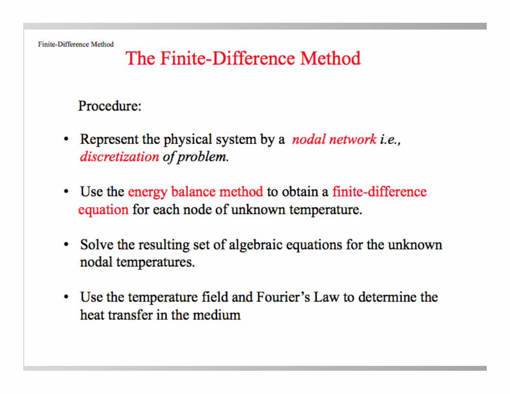
–  Steady\state&•  Essen7ally&

–  &Represent&the&physical&system&by&a&nodal&network.&–  &&Use&the&energy&balance&method&to&obtain&a&finite\difference&equa7on&for&each&node&of&unknown&temperature.&

–  &&Solve&the&resul7ng&set&of&algebraic&equa7ons&for&the&unknown&nodal&temperatures.&

boundary&nodes&

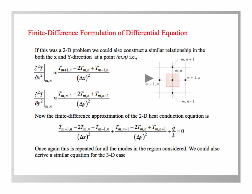
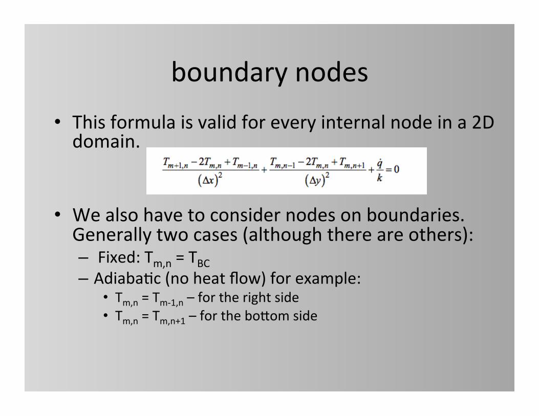
•  This&formula&is&valid&for&every&internal&node&in&a&2D&domain.&

•  We&also&have&to&consider&nodes&on&boundaries.&Generally&two&cases&(although&there&are&others):&–  &Fixed:&Tm,n&=&TBC&– Adiaba7c&(no&heat&flow)&for&example:&

•  Tm,n&=&Tm\1,n&–&for&the&right&side&

•  Tm,n&=&Tm,n+1&–&for&the&bofom&side&

A&set&of&equa7ons&

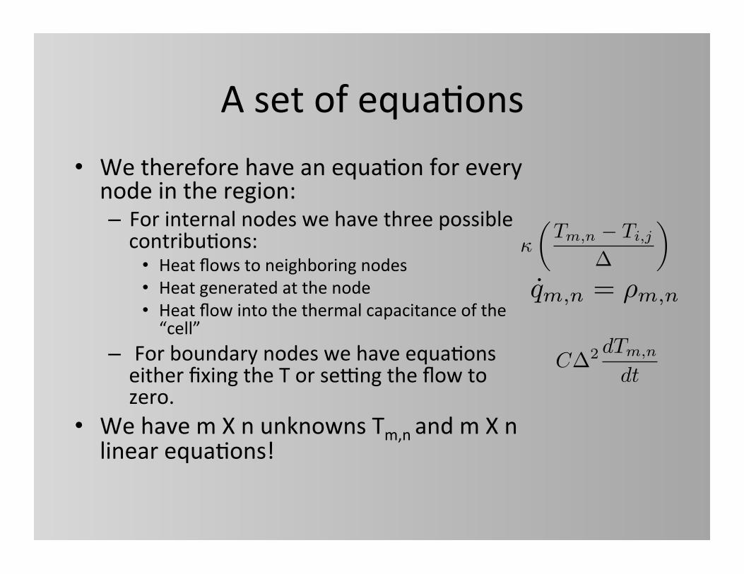
•  We&therefore&have&an&equa7on&for&every&node&in&the&region:&–  For&internal&nodes&we&have&three&possible&contribu7ons:&

•  Heat&flows&to&neighboring&nodes&•  Heat&generated&at&the&node&•  Heat&flow&into&the&thermal&capacitance&of&the&“cell”&

–  &For&boundary&nodes&we&have&equa7ons&either&fixing&the&T&or&segng&the&flow&to&zero.&

•  We&have&m&X&n&unknowns&Tm,n&and&m&X&n&linear&equa7ons!&

✓Tm,n � Ti,j

�

◆

qm,n = ⇢m,n

C�2 dTm,n

dt

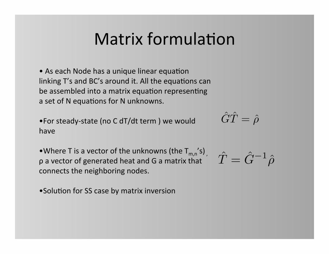
• &As&each&Node&has&a&unique&linear&equa7on&linking&T’s&and&BC’s&around&it.&All&the&equa7ons&can&

be&assembled&into&a&matrix&equa7on&represen7ng&

a&set&of&N&equa7ons&for&N&unknowns.&

• For&steady\state&(no&C&dT/dt&term&)&we&would&

have&

• Where&T&is&a&vector&of&the&unknowns&(the&Tm,n’s)&,&

ρ&a&vector&of&generated&heat&and&G&a&matrix&that&

connects&the&neighboring&nodes.&&&

• Solu7on&for&SS&case&by&matrix&inversion&

GT = ⇢

T = G�1⇢

Matrix&formula7on&

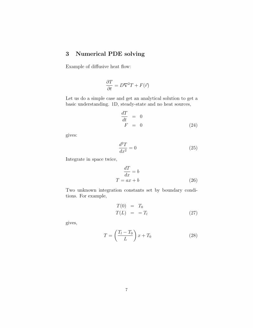
3 Numerical PDE solving

Example of di↵usive heat flow:

@T

@t

= Dr2T + F (~r)

Let us do a simple case and get an analytical solution to get abasic understanding. 1D, steady-state and no heat sources,

dT

dt

= 0

F = 0 (24)

gives:

d

2T

dx

2= 0 (25)

Integrate in space twice,

dT

dx

= b

T = ax+ b (26)

Two unknown integration constants set by boundary condi-tions. For example,

T (0) = T0

T (L) = = T

l

(27)

gives,

T =

✓T

l

� T0

L

◆x+ T0 (28)

7

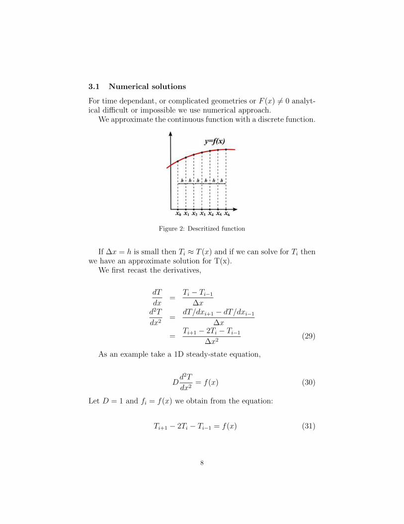
3.1 Numerical solutions

For time dependant, or complicated geometries or F (x) 6= 0 analyt-ical di�cult or impossible we use numerical approach.

We approximate the continuous function with a discrete function.

Figure 2: Descritized function

If �x = h is small then T

i

⇡ T (x) and if we can solve for Ti

thenwe have an approximate solution for T(x).

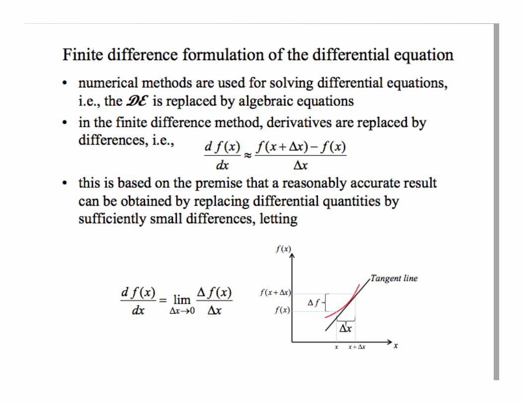
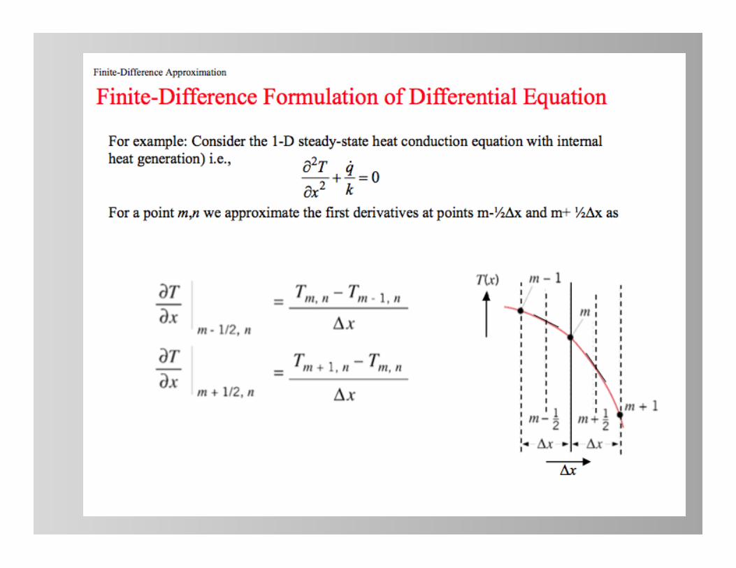
We first recast the derivatives,

dT

dx

=T

i

� T

i�1

�x

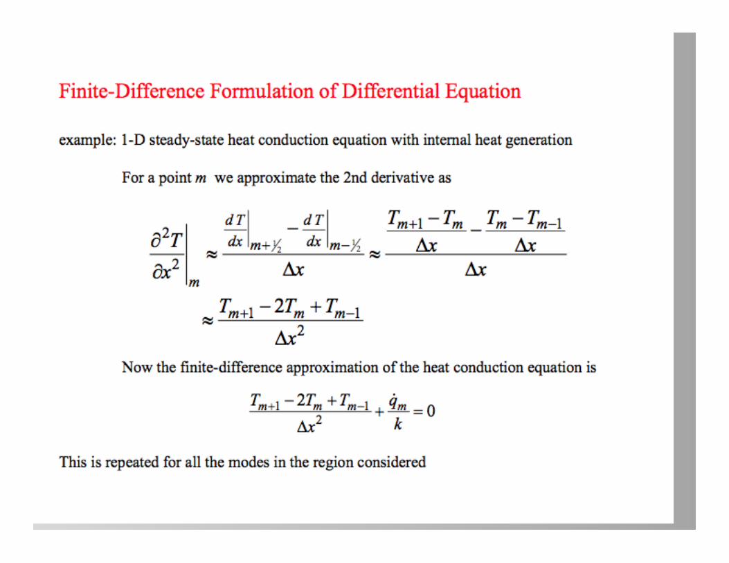
d

2T

dx

2=

dT/dx

i+1 � dT/dx

i�1

�x

=T

i+1 � 2Ti

� T

i�1

�x

2(29)

As an example take a 1D steady-state equation,

D

d

2T

dx

2= f(x) (30)

Let D = 1 and f

i

= f(x) we obtain from the equation:

T

i+1 � 2Ti

� T

i�1 = f(x) (31)

8

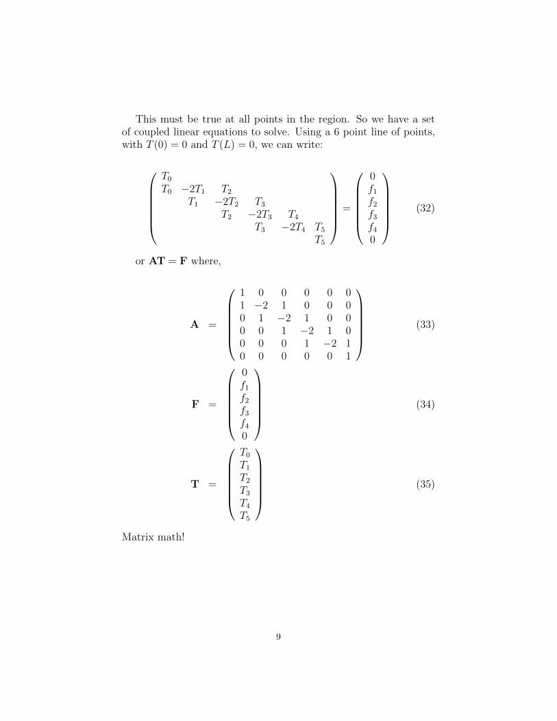
This must be true at all points in the region. So we have a setof coupled linear equations to solve. Using a 6 point line of points,with T (0) = 0 and T (L) = 0, we can write:

0

BBBBB@

T0

T0 �2T1 T2

T1 �2T2 T3

T2 �2T3 T4

T3 �2T4 T5

T5

1

CCCCCA=

0

BBBBB@

0f1

f2

f3

f4

0

1

CCCCCA(32)

or AT = F where,

A =

0

BBBBB@

1 0 0 0 0 01 �2 1 0 0 00 1 �2 1 0 00 0 1 �2 1 00 0 0 1 �2 10 0 0 0 0 1

1

CCCCCA(33)

F =

0

BBBBB@

0f1

f2

f3

f4

0

1

CCCCCA(34)

T =

0

BBBBB@

T0

T1

T2

T3

T4

T5

1

CCCCCA(35)

Matrix math!

9

We can solve this set of equations on a computer. Let �x bevery small and the number of points large (100’s to millions) andwe can solve complicated problems like this using programs such asMatlab.

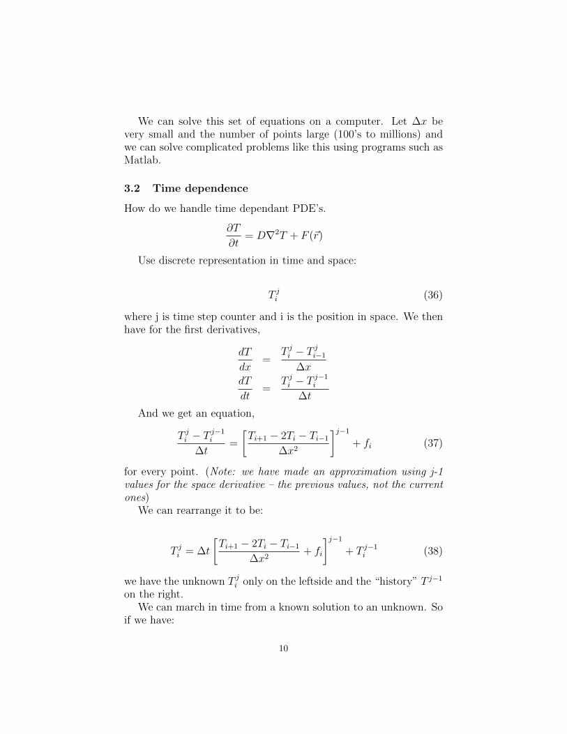
3.2 Time dependence

How do we handle time dependant PDE’s.

@T

@t

= Dr2T + F (~r)

Use discrete representation in time and space:

T

j

i

(36)

where j is time step counter and i is the position in space. We thenhave for the first derivatives,

dT

dx

=T

j

i

� T

j

i�1

�x

dT

dt

=T

j

i

� T

j�1i

�t

And we get an equation,

T

j

i

� T

j�1i

�t

=

T

i+1 � 2Ti

� T

i�1

�x

2

�j�1

+ f

i

(37)

for every point. (Note: we have made an approximation using j-1

values for the space derivative – the previous values, not the current

ones)We can rearrange it to be:

T

j

i

= �t

T

i+1 � 2Ti

� T

i�1

�x

2+ f

i

�j�1

+ T

j�1i

(38)

we have the unknown T

j

i

only on the leftside and the “history” T

j�1

on the right.We can march in time from a known solution to an unknown. So

if we have:

10

T

j=0i

= Some known distribution (39)

T

j

Boundarys

= Boundary values (40)

we can compute from a known history to the future.Many issues and problems but this sort of approach is the heart

of many computer aided design tools.

11

Solu7on&Methods&

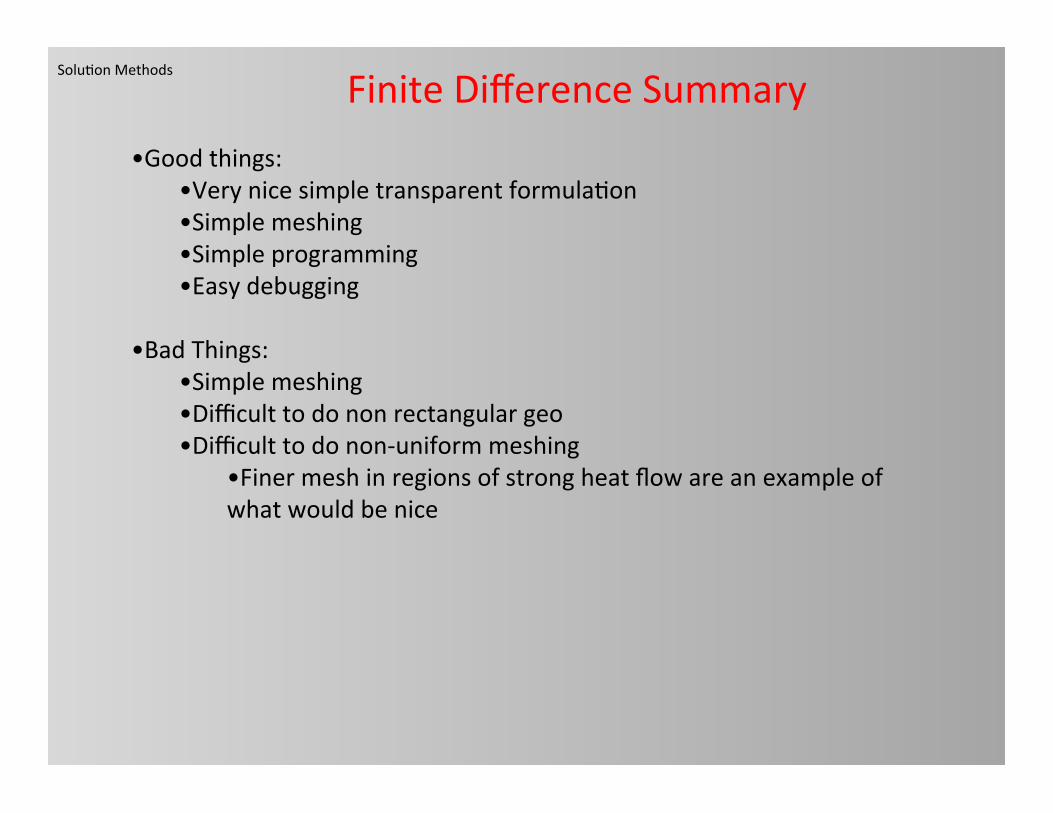
Finite&Difference&Summary&

• Good&things:&• Very&nice&simple&transparent&formula7on&

• Simple&meshing&

• Simple&programming&

• Easy&debugging&

• Bad&Things:&• Simple&meshing&&

• Difficult&to&do&non&rectangular&geo&

• Difficult&to&do&non\uniform&meshing&

• Finer&mesh&in&regions&of&strong&heat&flow&are&an&example&of&

what&would&be&nice&

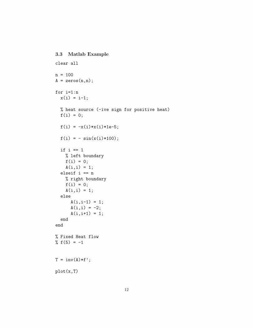
3.3 Matlab Example

clear all

n = 100

A = zeros(n,n);

for i=1:n

x(i) = i-1;

% heat source (-ive sign for positive heat)

f(i) = 0;

f(i) = -x(i)*x(i)*1e-5;

f(i) = - sin(x(i)*100);

if i == 1

% left boundary

f(i) = 0;

A(i,i) = 1;

elseif i == n

% right boundary

f(i) = 0;

A(i,i) = 1;

else

A(i,i-1) = 1;

A(i,i) = -2;

A(i,i+1) = 1;

end

end

% Fixed Heat flow

% f(5) = -1

T = inv(A)*f’;

plot(x,T)

12

Finite&Element&Modeling&

• More&flexible&then&FD&with&respect&to&geometry&

• Many&areas&of&applica7on&

• Electromagne7c&

• Stress/Strain&• Heat&flow&• Etc.&

• Example&of&stress\strain&stolen&from&Biomedical&engineering&

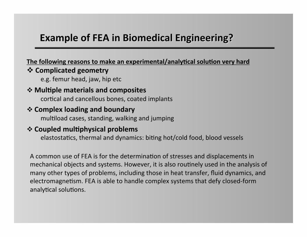
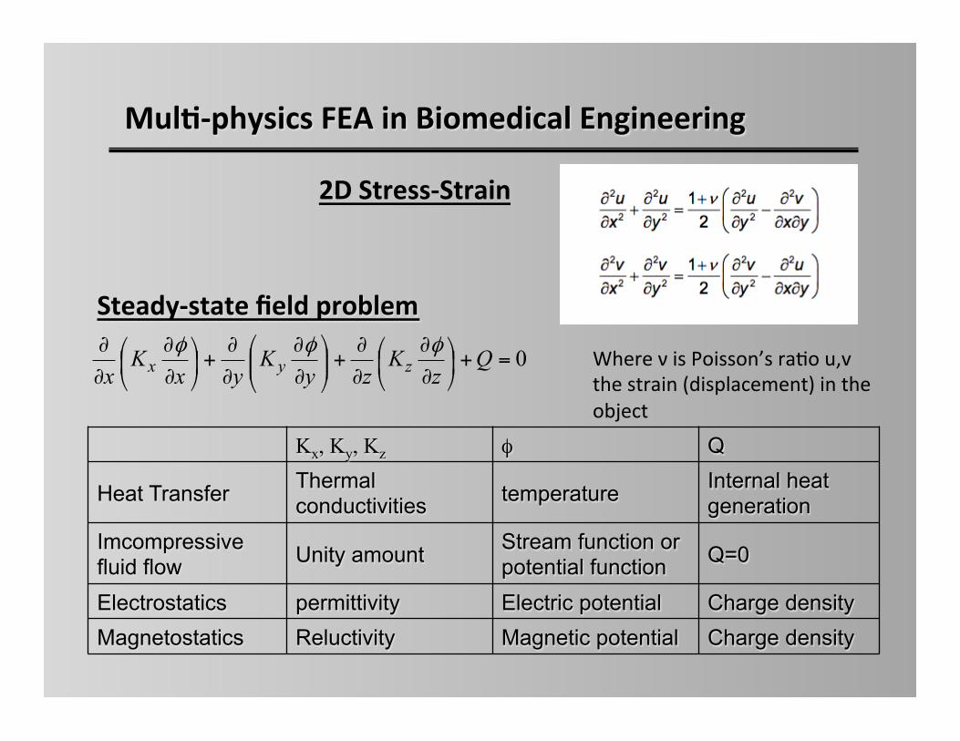
Example(of(FEA(in(Biomedical(Engineering?(((

A&common&use&of&FEA&is&for&the&determina7on&of&stresses&and&displacements&in&

mechanical&objects&and&systems.&However,&it&is&also&rou7nely&used&in&the&analysis&of&

many&other&types&of&problems,&including&those&in&heat&transfer,&fluid&dynamics,&and&

electromagne7sm.&FEA&is&able&to&handle&complex&systems&that&defy&closed\form&

analy7cal&solu7ons.&

The(following(reasons(to(make(an(experimental/analy=cal(solu=on(very(hard&! (Complicated(geometry(

&e.g.&femur&head,&jaw,&hip&etc &&

! &Mul=ple(materials(and(composites&&&cor7cal&and&cancellous&bones,&coated&implants&

! &Complex(loading(and(boundary((&mul7load&cases,&standing,&walking&and&jumping&

! &Coupled(mul=physical(problems( ((&elastosta7cs,&thermal&and&dynamics:&bi7ng&hot/cold&food,&blood&vessels&

0=+!"

#$%

&∂∂

∂∂

+!!"

#$$%

&∂∂

∂∂

+!"

#$%

&∂∂

∂∂ Q

zK

zyK

yxK

x zyxφφφ

Mul=Cphysics(FEA(in(Biomedical(Engineering(

Kx, Ky, Kz φ Q

Heat Transfer Thermal conductivities temperature Internal heat

generation Imcompressive fluid flow Unity amount Stream function or

potential function Q=0

Electrostatics permittivity Electric potential Charge density Magnetostatics Reluctivity Magnetic potential Charge density

SteadyCstate(field(problem(

2D(StressCStrain(

Where&ν&is&Poisson’s&ra7o&u,v&

the&strain&(displacement)&in&the&

object&

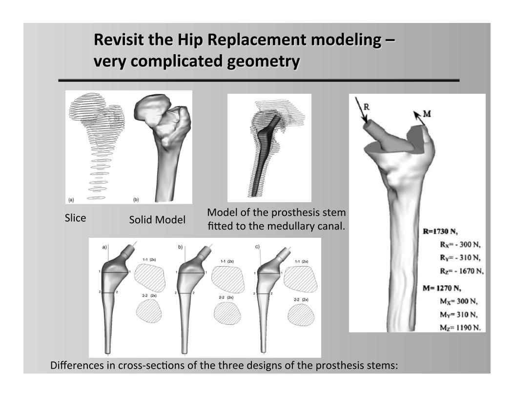
Revisit(the(Hip(Replacement(modeling(–((very(complicated(geometry((

Slice&Model&of&the&prosthesis&stem&

fifed&to&the&medullary&canal.&

Differences&in&cross\sec7ons&of&the&three&designs&of&the&prosthesis&stems:&

Solid&Model&

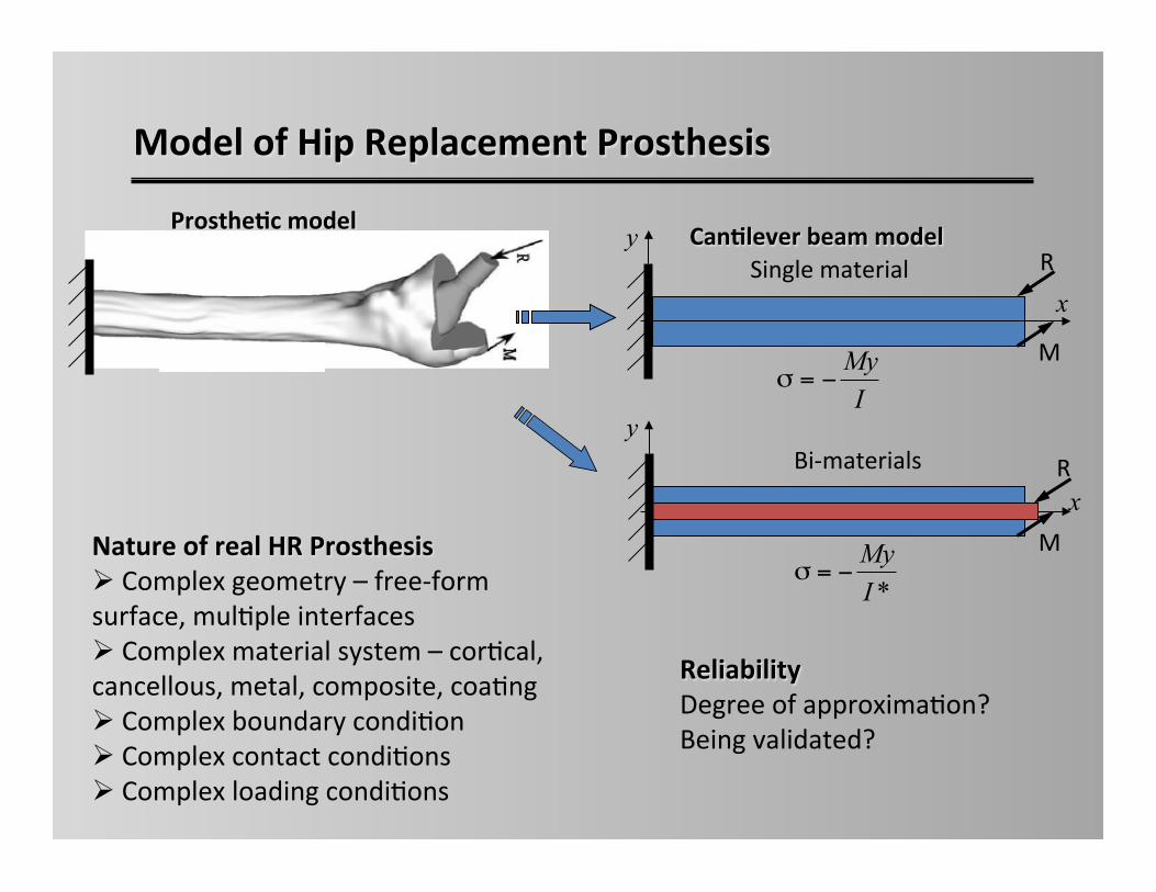
Model(of(Hip(Replacement(Prosthesis(

Nature(of(real(HR(Prosthesis(" &Complex&geometry&–&free\form&

surface,&mul7ple&interfaces&

" &Complex&material&system&–&cor7cal,&

cancellous,&metal,&composite,&coa7ng&

" &Complex&boundary&condi7on&

" &Complex&contact&condi7ons&

" &Complex&loading&condi7ons&&

Prosthe=c(model( Can=lever(beam(model(

IMy

−=σ

R&

M&

y

x

*IMy

−=σ

R&

M&

x

Single&material&

Bi\materials&

y

Reliability(Degree&of&approxima7on?&

Being&validated?&&

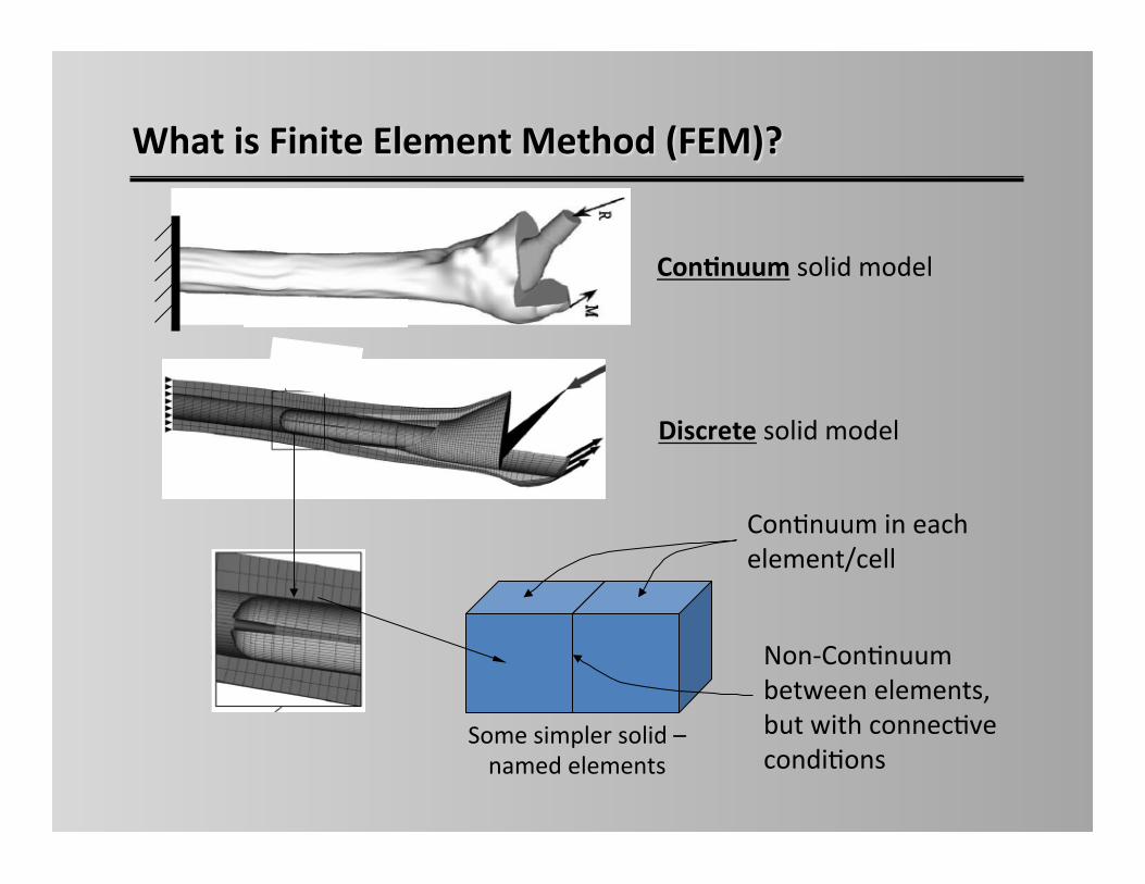
What(is(Finite(Element(Method((FEM)?(

Con=nuum&solid&model&

Discrete(solid&model&

Some&simpler&solid&–&

named&elements&

Con7nuum&in&each&

element/cell&

Non\Con7nuum&

between&elements,&

but&with&connec7ve&

condi7ons&

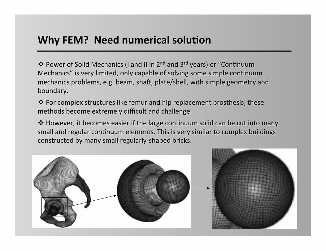
Why(FEM?((Need(numerical(solu=on((

! &Power&of&Solid&Mechanics&(I&and&II&in&2nd&and&3rd&years)&or&“Con7nuum&

Mechanics”&is&very&limited,&only&capable&of&solving&some&simple&con7nuum&

mechanics&problems,&e.g.&beam,&shaM,&plate/shell,&with&simple&geometry&and&

boundary.&&

! &For&complex&structures&like&femur&and&hip&replacement&prosthesis,&these&

methods&become&extremely&difficult&and&challenge.&&

! &However,&it&becomes&easier&if&the&large&con7nuum&solid&can&be&cut&into&many&

small&and&regular&con7nuum&elements.&This&is&very&similar&to&complex&buildings&

constructed&by&many&small&regularly\shaped&bricks.&

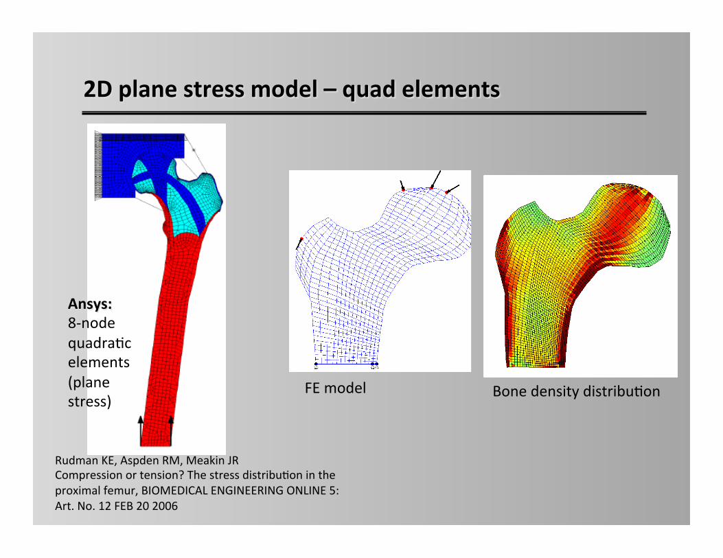
2D(plane(stress(model(–(quad(elements((

Ansys:&&8\node&

quadra7c&

elements&

(plane&

stress)&

Rudman&KE,&Aspden&RM,&Meakin&JR&

Compression&or&tension?&The&stress&distribu7on&in&the&

proximal&femur,&BIOMEDICAL&ENGINEERING&ONLINE&5:&

Art.&No.&12&FEB&20&2006&&

FE&model& Bone&density&distribu7on&

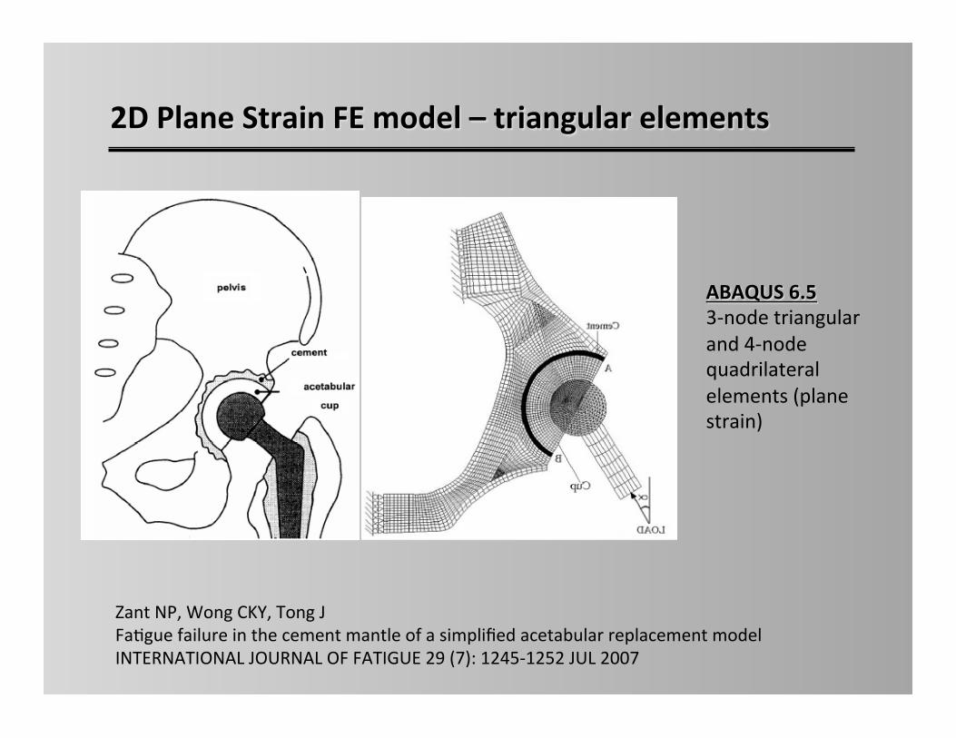
2D(Plane(Strain(FE(model(–(triangular(elements((

Zant&NP,&Wong&CKY,&Tong&J&

Fa7gue&failure&in&the&cement&mantle&of&a&simplified&acetabular&replacement&model&&

INTERNATIONAL&JOURNAL&OF&FATIGUE&29&(7):&1245\1252&JUL&2007&&

ABAQUS(6.5(3\node&triangular&

and&4\node&

quadrilateral&

elements&(plane&

strain)&

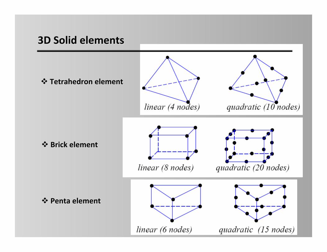
3D(Solid(elements(

! (Tetrahedron(element(

! (Brick(element(

! (Penta(element(

Solu7on&Methods&

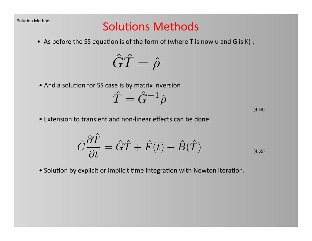
Solu7ons&Methods&• &&As&before&the&SS&equa7on&is&of&the&form&of&(where&T&is&now&u&and&G&is&K)&:&

(4.53)&

• &And&a&solu7on&for&SS&case&is&by&matrix&inversion&

• &Extension&to&transient&and&non\linear&effects&can&be&done:&

• &Solu7on&by&explicit&or&implicit&7me&integra7on&with&Newton&itera7on.&

(4.55)&

GT = ⇢

T = G�1⇢

C@T

@t= GT + F (t) + B(T )

Solu7on&Methods&

Finite&Element&Summary&

• &Bad&things:&• Very&difficult&and&unintui7ve&formula7on&

• Complicated&meshing&

• Difficult&programming&

• Not&easy&debugging&

• &Good&Things:&• Flexible&complicated&meshing&&

• Easy\ish&to&do&non&rectangular&geo&• &Easy\ish&to&do&non\uniform&meshing&

• Finer&mesh&in&regions&of&high&stress.&