FIFTH INTERNATIONAL CONGRESS ON SOUND AND VIBRATION

DECEMBER 15-18, 1997ADELAIDE, SOUTH AUSTRALIA

Resonant oscillations governed by the Boussinesq equation with damping

Sh.U.GalievDepartment of Mechanical Engineering, The University of Auckland, Private Bag

92019, Auckland 1, New Zealand

Abstract. It is shown that the perturbed Boussinesq type equations describe oscillations indifferent porous media (soils, rocks, bubbly liquids and so on). Nonlinear earthquake-inducedvertical and horizontal waves in natural resonators (hills, basins and so on) are studied.Periodical resonant solutions of the above equations are constructed by the perturbationmethod. The solutions display on the one hand generation and interaction shock-, solitary- andcnoidal-type waves and on the other weak nonlinear interaction left-and right-hand sidetraveling waves. Traveling oscillons which can form standing oscillons are discussed.Nonlinear, off-resonant dispersive, hysteresis, trap, topographical and dissipative effectswhich can take place in the natural resonators during earthquakes are defiied. Theoreticalresults explain some anomalous data from the Northridge 1994 Southern Californiaearthquake and also data of earthquake modelling.1. Basic equations for the ground layerMany of the world’s cities are built on sedimentary basins or at the tops of ridges or nearwater basins. From the standpoint of earthquake risk, however, basins (valleys), hilltops andcoastal regions are often the least desirable places to build. The topographies can form naturalresonators, where seismic waves are amplified to shattering intensity. lleo~tical calculationspredict that crest amplillcations with respect to the base can reach a factor of 30. Theresonance of seismic waves in sedimentary basins was the reason for the collapse of about 300buildings during the 1985 Mexico City earthquake [1]. A peak acceleration of 1.82g wasrecorded [2] during the Northridge 1994 Southern California earthquake. This recordarnp~lcation of the ground motions at the Tarzana hill maybe also explained by the resonance.Earthquake-induced oscillations of a bed (bottom) can generate a train of tsunami-like waves.1.1. Surjace wavesRecently there has been great interest in the physics of sand-like material lying on a verticallyoscillating surface [3,4]. Different, very interesting wave phenomena were observed on thelayer surface depending on the amplitude and frequency of excitation. These phenomena wereusually connected with the parametric effect. However there are a possibility of a verticalexcitation of the surface ground waves due to a topographical effect.Following Airy’s method [5, p. 259] we can write equations of motion and continuity for aviscoelastic (the Kelvin model) surface layer

p hua =cYx(h+q) , I’z=(h+q)(l+ux) , (1.1)

where t istime, x is a horizontal Lagrangian coordinate, u is a horizontal displacement, p is

the density, his a variable thickness of a surface layer of the ground ( h= h{ x)), o is a stress,q denotes an elevation of the surface, P is a hydrostatic pressun?, and subscripts t and x,respectively, indicate the time and space derivatives. Let us assume that the some contributionto c comes from the hydrostatic law which is the basis of the theory of shallow water waves.One can find, following this theory [6] and neglecting the difference between Lagrangian andEulerian coordinates for small values that:

cY=- Pg(~– Y+n)–pgk2(h+@= /3+41.1*ux/3+4q*zfm /3. (1.2)

where hois an averaged thickness of the layer and (h-hO)/hoeel, p“ is an elastic shearmodulus, q“ is a viscosity coefficient. A subscript Odefines here and further undisturbedvalues. Below we will not take into account the fourth order, with respect to u, terms in (1. 1)and (1.2). Moreover, nonlinear terms will be only considered which do not explicitly dependon the viscosity and dispersive coefficients. We assume that g = go + gy, where go is the

acceleration due to gravity, and gYis the seismic-induced acceleration. It is also assumed thattopographic terms similar to pghXuXand less are negligible. This simpliiles the analysis of the

influence of the nonlinearity, resonance and topography on the surface waves. Taking intoaccount the comments above one can obtain from (1.1) and (1.2) that

Un– a: u= = ~uxu= + j$u=u: + Puti + kum - ghx- g~hm f 3, (1.3)

where a~=a~+4p*p-1 /3, a~=gh, ~=–3gh, ~1=6gh, lJ=4~*p-1/3 and

k = gh~a~2/ 3. The speed, aO, of the shallow ground waves depends on the thickness of the

layer and on the shear-wave speed. a o also depends on a perturbation gYof g but we willneglect this dependence. If p“ =0 equation (1.3) is valid for water waves. The nonlinear termsin (1.3) are of the second and third order. Generally speaking, the dissipative term is of fustorder but we will assume that this term and kum are of second order. The last terms in (1.3)

take into account the topographic effects. The perturbation method allow to obtain theapproximate solution of (1.3) [7]:

u= J1(r)+jl (s)+.12(r) +j2(s)+Jq(r)+js($)

//-0.25a-1 g[h~-h, + ~2a-2(h~~- 3h~r+ 3hm~– hm,)/ 31drak

+A(r – s){[J~(r)]2 +[ j~(s)]2 }/ 2+ IUZ;2(S–r)[.l~(r) - j~(s)li 4

+kqz (s – r)[J~ (r) – j~(s)] / 4 + A(r– s)[J;(W; (r) + j; (s)jj(dl (1.4)

+a{jl (s)[J~(r)]2 + J, (r)[j~(s)12 }12 + @- A2 / 2){Ji(~)~[ji(s)12ds +.ji(S)~[Ji(~)12 dr}

+(c – 3A*/ 2)(r – s){ [j~(s)]3– [.l~(r)]3} + A2(r2 – 2rs+ s2){.l; (r)[J;(r)]2+ j~(s)[j~(s)]2}.

Here J1(r),jl (s), J2(r), j2 (s), JJ(r),j~ (s) are unknown functions defined by bo~dary

conditions, A = f!a;3/ 4,a = 5A2– 2D,b = –2A2 + D,c = -4a2 + D,D = ~1/ 4a$ and

r=t–xa;1+~ua;3/4 and s=t+xa~l - @a;3 /4. Expression (1.4) is only valid forperiodical processes.1.2. Vertical wavesIf the thickness of the topographies increases then vertical waves are excited additionally to thesurface waves. Let us consider these waves assuming that the thickness is much lesser thenother dimensions of the hill (basin). So that to simplify the problem we will consider thevertical waves as independent from the surface waves and neglect by a variation of the

thickness of the hill (basin). Therefore the vertical waves maybe considered as one-dimensional waves which propagate in the layer with parallel flat surfaces. Material of the layerwill be simulate as a granular viscoelasic (the Kelvin model) medium saturated by the air-liquidmixture.After the above assumptions our problem is reduced to a solution the next equations which arewritten for average values:

poun =6. , (1.5)

po+ @ = plJ , (1.6)

6= –P+4~*(l+F2vo -nv)ux /3+4q*ux /3 , (1.7)

P =po[(l-~vo)(l-P/K~-~/KB) +nv]-’, (1.8)

P, -B? = klrI;lrI1(l-otB)px , (1.9)

(p+ Y)(p, + n-’ = (p, / p,,)’, (l.lO)

where (1.5)-(1.9) are the motion, continuity, constitutive, state and hydraulic diffusivity [8]equations, respectively. Equation (1.10) is a state equation for bubbly liquid saturating ofpores. In (1.5)-(1 .9) x is a vertical and upwards Lagrangian coordinate; P is a pressure in thesolid phase, respectively. Writing equation (1.7) we considered the granular material as theinitially damaged material and took into account an influence of a variation of the damages(pores) on this equation [9]. We assumed that nV is of the porous volume per unit volume ofthe material. The state equation (1.8), where p is a pressure of the porous liquid and K~ is the

bulk modulus of the equivalent dry material [8] is an analog of the state equation for bubblyliquid [10]. Following [8] we wrote the hydraulic diffusion equation (1.9) introducing the‘Skempton’s coefficient’ B, permeability coefficient kl, Biot’s modulus~, Biot’s coefficient

a, and viscosity coefficient q* of bubbly liquid. We will study only compression-tensionprocesses in plane waves therefore a liquid motion is connected with a change of the materialvolume. As a result there is the practically undrained deformation of the layer material in theabove waves. Equation (1.10) was written following [11]. Value pl is the average density ofbubbly liquid and

Kf(l–vog)+v-og/(we)-PO ,

y = (k+ 1)(1-VO,)K; +V&(’y+ l)y-2p;2 -[Kf(l -vO,) +Vog/ (W?J12

z= {[ ~f(l–vllg)+vog MPO)I(PO+W}”l $ K, = [L(po + B.)]-l ,

where Vi , A and y are the undisturbed volume of gas bubbles per unit volume of the liquidand the polytropic exponents of the fluid and air, respectively. Value B* is a constant. Forroom temperature k =7.15 and B*= 304.5 MPa. In the case of adiabatic oscillations ofbubbles y= 1.4, and y= 1 in the case of isothermal ones. Assuming in (1.10) the gas volumeVo~= O or 1 we can obtain the state equation for fluid or gas, respectively. Since mass of the

bubbly liquid in pores does not vary, a variation of the density of this liquid is defined by avariation of volume of the pores. Therefore we can rewrite equation (1.10) as(p+ Y)(po + Y)-’ = (V./v)z. (1.11)

It is emphasises that equations (1.5)-(1.9) and (1.11) describe waves in bubbly liquid if p.” =0,kl =0 and a =0. Equations (1.5)-(1.9) and (1.11) can be reduced to

2= fkxu= + p,u=zf: + W& , (1.12)

;h=~~ = (4P* /3-blB-’)p~’ , ~ = --4P*P~1[l+b1K~ + 152B-1 / P*I J 3,

b,= -P;[4P*~2JQ13+ WJ-11 ~ P =WI* iq+w’l:h,w -@%21Pii’ and

K; = (l–vo)(l?-l +a)K;l , bl = –Z(po + Y)VO-l[l+Z(po + Y)VO-lK;l]-l,

bz = ~.5(Z + l)blVO-l[l+ b1K;]2 , b~= 05(2+ l)bl~-2[a1(z+ l)K~ + (Z+ 2) / 3][l+b1K~]3 .

Constitutive equation (1.7) maybe written so that:

a= -(b,ux +b2u:+b,u:) / B + kqlq-l(B-l –cO~ (4uX+b2u; +bqu:)udt + 4p*[l – UX

-K:(bluX +b2u:)]ux / 3+ 4rI*UN/ 3 . (1.13)

Equation (1.13) is valid for the weakly nonlinear granular media. But inside of the Tarzana hillthe accelerations were close to 2 go and strong nonlinear waves should be expected.Particularly, granular media (soil) demonstrate the different behaviour in tension andcompression waves. In the tension waves the soil properties remind properties of bubbly liquidor gas. If an excited acceleration is greater than go, the resonator can periodically lose acontact with the bed. As a result the seismic waves are trapped by the resonator.A strongly nonlinear const.itutive equation was written for the dry undrained inviscid material:

6= &B-l {b - [b2+ 4~VOK;]o”5}+ 4p*ux/ 3, (1.14)

where b = Ux+ V. - PoK~ . According to (1.14) properties of the granular-type material inside

of the tension waves is close to properties of gas. Equation (1.14) is an analog of the stronglynonlinear state equation discussed in [12] for water.If h,= k =0 then equation (1.3) reduces to (1.12) and solution (1.4) is the solution of equation(1.12). Solution (1.4) is approximately valid both for elongated hills and valleys (basins)because we are modelling them as the infinite layer. However, we will mostly discuss theground motion at the Tarzana hill. It is important for our model that the P-wave velocity ~‘inside’ of the Tarzana hill is approximately 520 rnh [2] while the P-wave velocity is 1100mh just 5 m below the base of the hill. Thus, near this base there is the P- wave velocitydiscontinuity. The seismic waves reflect practically completely from this discontinuity and as aresult they am trapped by the hill.2. Simulation of resonators with free boundary (hills and basins)First, the horizontal waves in the hill is considered. The length of the hill is 2L. Theundisturbed hill surface is defined by the equality y=h(.x).The bottom of the hill is at y= O.Let a hill geometry be symmetrical with respect to the vertical x = O,and y=h(0) is the highestpoint of the hill top. A slope of the hill top with respect to the bottom of the hill is constant andvery small (hx=aeel). Lateral surfaces of the hill are perpendicular to the hill bottom andlocated at ~ *L. Let the seismic-induced vertical acceleration be approximated by theperiodical law: gY= 6 coscot.At the lateral surfaces of the hill we have 6 = O. The hill issymmetrical therefore u = O (x= O) , a = O (x= L). Finally the boundary conditions maybe

presented so thatu= O(X=O) , UX=O (x= L). (2.1)Let us consider the basin (valley). It is assumed that a basin free surface is flat, but the centralpoint of the basin bottom is a lowest point of this surface. The point x =0 we locate at the leftflank of the basin. The flanks are freed. As a result the displacement u =0 at x= Oand at x= 2L.Since the problem is completely symmetrical with respect to x= L we have there u, = O. So

the last problem is identical to the problem formulated above for the hill.Considering the vertical waves we assume that the ground surface is free and the underlyingsurface of the layer is excited harmonically:u,=-@Zsincot(x=O) , UX=O (x= L). (2.2)One can see that the formulated above problems for the vertical and horizontal waves are thesame since hx is constant and gY= 6 cos(ot for the horizontal waves. An expression definingthe resonant frequencies follows from the linear solution of the problem:

QN = (ZV-1/2)na0 / L (N=l, 2,3, ..). (2.3)Together with (2.3), according to the nonlinear correction of the linear solution, there are theso-called quadratic resonant frequencies:Q; =( N-1/2)mz0/2L . (2.4)

We must emphases that expressions (2.3) and (2.4) are valid both for horizontal and verticalwaves but ao and L are fifferent vary for those cases.Let us calculate the f~st two resonant frequencies of the hill using formula (2.3) which takesinto account both the height and length of the Tarzana hill. Following [2] we will take thelargest (L.=250 m) and smallest (L=1OOm) dimensions of the hill and assume that the shear-wave speed equal to 249 rids. Then for L =250 m we have f21= 1.77 and Q2=5.3 Hz. These

values correlate well with frequency peaks presented in Fig. 6 from [2]. For L =100 m wehave Q,= 4.42 and Q2=13.2 Hz. The frequency Ql = 4.42 Hz correlates with main frequency

peak (3.26 Hz) presented in Fig. 6 from [2]. It is easy to find from (2.3) the dimension (L =139m) of the hill which comesponds to the above main frequency peak. For this dimension ( thedimension depends on the direction of measuring the hill) we have f21= 3.26 and Q= 9.78

Hz. The last value correlates with the second main frequency peak (8.6-8.8 Hz). Rail [2]identiiles this peak as a possible f~st vertical overtone. However, the average P-wave velocitybetween the base and the top of the hill was 578A60 m/s, therefore we explain the abovesecond main frequency peak by the second resonance of the horizontal oscillations. So theformula (2.3) describes some results of the calculations and observations,Let us construct solutions which are valid near and at resonances (2.3) and (2.4). For theresonant frequencies (2.3) and p =0 the boundary conditions give the next basic equation:-w*F’ – ka~3LF””+ q-3L(F’)3 / 8 = zCOS(Dt . (2.5)

Here F’ = J;(t + L / aO) andw*F’ takes into account contributions from the off-resonance

effects. First we consider the nonlinear effect. If co”=k=(l we haveF’(t*(x– L)/aO) = 2aO[lL-1cosco(t*x/aO)]l’3 . (2.6)

Now the elevation and horizontal acceleration may be calculatedq=~F’(r +L/aO)- F’(s– L/aO)]/aO, UM=F’’(r+ L/aO)+F’’(L-aO)O) (2.7)

The expression for F“ (which is valid if the influence of the dispersion on equation (2.5) is

small and localises at and near m = m - arccosll? , where R = -2s’3aOco*(L12)-1’3/ 3 ) is

F’ = 4aO(m*co-l)Os@(t+ Lujl)[l – O(t + LA# )] +2a0(lL-l)113y . (2.8)

Here @(t + Lu~l) = tanh[-aOco-l(o)“co‘lk-l )05cos(cot+ arcco~Rl)] and it is assumed that

aoco-l(co*o-lk-l )05>>1. If R M we have in (2.8) that

Y= -2R1 sinh[~a sinh(05R1-3coscot)], (2.9)

where RI = 2-1’3(@zcos@14°”5 . Expression (2.9) is valid behind the resonant frequency

where o.)*cO. If -1< R< O(m”>0) there is no continuous single-valued solution for y, andit is necessary to accept solution with discontinuties:

Y= -2R1 cosh[@ccosh(05R1-3 coso)t)] ; -2R1 cos[@ccos(05R~3 coso)t)] ;

–2R1cos[@ccos(05R1-3 coscot) + 2X / 3]; -2R1 cosh[@ccosh(05R1-3 coscot)] ;

“–2R1cos[~arccos(05R1-3cosmt) + 2X / 3];-2R1 cos[~ arccos(05R1-3CoS@t)] s

-2R1 cosh[$ arccosh(05R1-3coso)t)] , (2.10)

which isvalid for Oecot<arcco~R ; arcco~R co)t Sz/2; n/2<cot<z-arcco~R ;

n-amco@ <cot Sn+amcos@; n+arccos@ cw<2n/3;3n/2 <ot<27c-arcco4R;

27c- arcco~lll c cot S 2X, respectively.

If R e- 1 there are three continuous expressions for y:

Y= –2R1 cos[#acos(05R~3 Cosolt)+ 2(i - 1)7C/ 3], i =1;2;3. (2.11)

It is to be emphasised that there is also the acoustic solution. Generally speaking, the fmt termin (2.8), which takes into account dispersion, maybe very small. Solution (2.8) describesshock-like waves generated if - ldl<O. Thus, solution (2.8) is not symmetrical respectivelyresonant fnxpency.Generally speaking, acoustics and nonlinear (2.8) solutions may be used for description ofdifferent scenarios an off-resonant evolution of waves. Particularly they take into accounthysteresis in earth material under dynamic resonance discussed in [13]. In Figures 1 and 2 anevolution of the resonant elevation wave is presented when the excited frequency increasesand decmises through a resonance, respectively. The amplitude 1=104 m. The curves (*****)were calculated according to the acoustic solution. The other curves were calculated accordingto (2.8). The intensive shock-like waves are generated if the excited frequency decreases (seeFig. 2).Now using (2.7) we can write expressions for the resonant traveling waves. For example, forthe traveling waves of the acceleration we haveF“’[t+(x - L)/aO] = 4a@*Co-1k4”5sinolp. sech2[-aOol-1(co*o.)-lk-l)03cosw. ]

+2ao (U-l )1’3yt (t + x / a. ) , (2.12)

where p. =tAx/ao+o) ‘1arcco~R . The f~st term in (2.12) takes into account the dispersive

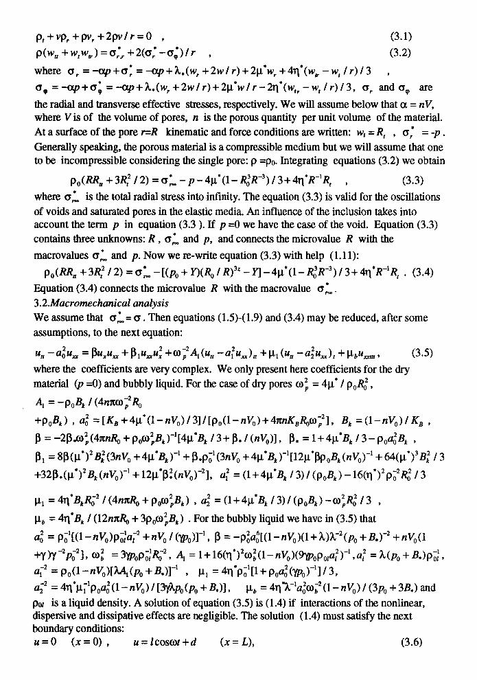
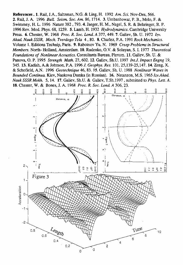
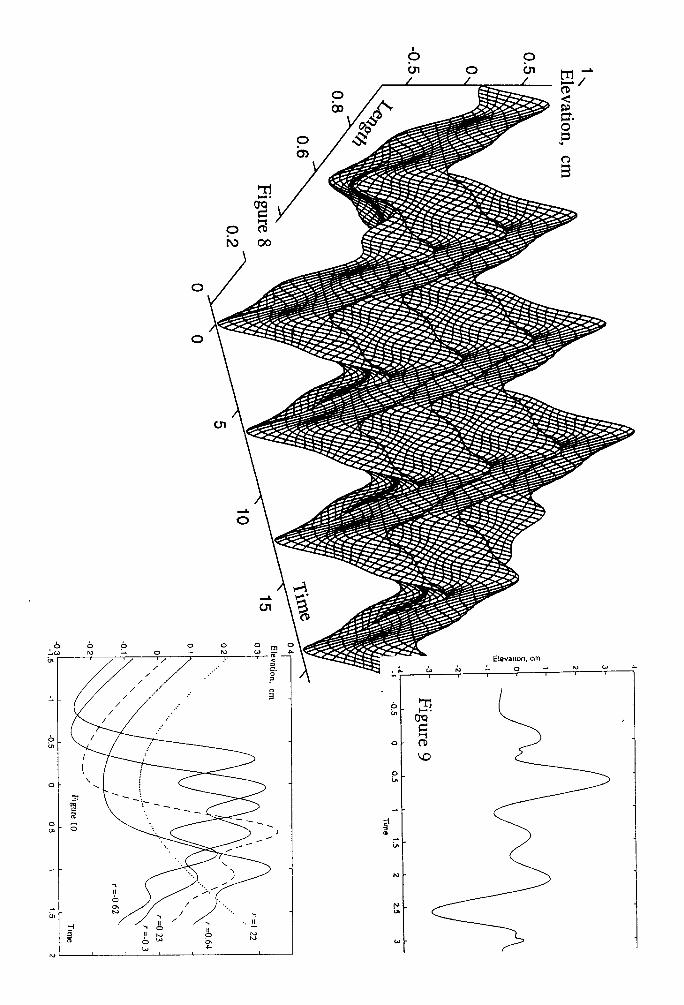
effect which accumulates near lines where up. = m. One can see that the dispersive effect isvery important for acceleration waves. Particularly, the fust term in (2.12) maybe larger thanthe second term. Expressions (2.8) and (2.12) are valid if R e O(CO*>0). For case R> O (co”cO) the fust terms in (2.8) and (2.12) are absent.From (2. 12) it is follows that during the half period of the excitation the traveling waves recallsolitons (peaks) and at the next half of the excitation the traveling waves recall antisolitons(crates) exist. These oscillating excitations recall so-called, recently experimentally discovered,oscih?ons[3]. By contrast with oscillons solution (2.12) describes traveling oscillons.In Fig. 3 the traveling oscillon is presented. We assumed that R =0.3, 1=104 m and L= 139m, h =20 m. The dimensionless time at is used. The length is 1-x-AZand N =1. The right-handside half of the hill is considered. One can see in Fig. 3 the oscillon traveling up to the hilltopand down to the lateral surface of the hill. We recall that the wave, which is symmetricalpresented in Fig. 3, exists on the left-hand side of the hill. An maximum amplitude of thewave is approximately equal to the peak of the acceleration at the Tarzana hill. This maximumis on the flank of our pattern, where peaks follow after craters and vise versa. This maximumreduces and the oscillation profde varies when the distance from the lateral surface increases.At approximately x=U2 the oscillations reminiscent of a shock wave having two peaks aregenerated. An increase the distance leads to steepening of those waves. Thus, according to thetheory, the largest resonant amplKlcation of the acceleration takes place near the edges of thepattern. However, this amplification may be very local and it affects only high harmonics. Nearthe centre of the hill the ampli13cationmay be smaller but affects both high and low frequencyharmonics. In Fig. 4 the curves are presented which were calculated for R =-0.3 at x =0.9 L (_) andx=L/2(--- -). For us it is important that the some curves in Figures 3 and 4 arepractically the same as the shock-like and oscillon-like oscillations excited during of earthquakemodelling (see Figures 14, 16, 18 and 21 from [14 ]).Quantity of the oscillons, traveling up and down along of the hill, depend on the excited

frequency and equal 2N. They can form different patterns. One of them, calculated for R =0.0.5,1 = 104 m and N =4, displays in Fig. 5. One can see that along of the hill the standingoscillons are organised as a result of collisions of the traveling oscillons. A generation of theseoscillons reminds the generation of the standing waves in linear acoustics but here we havenonlinear effect and the standing oscillons maybe very strongly localised on the surface of thehill.M us consider earthquake-induced waves near the quadratic resonant frequencies (2.4). Theboundary conditions give the next basic equation if the dissipative effect is negligible:F’l + F’l –2A(F_1F~1– F’+lF”l)= -o.)lshmt . (2.13)

Subharmonic oscillations are generated in a granular media under vertical vibrations if theacceleration amplitude larger than gO[3,4]. Since the peak acceleration of 1.82 gOwas

recorded at Tarzana hill we will try to consider strongly nonlinear effect, namely, thesubharmonic oscillations of the topographies. Of course, our theories are not valid for stronglynonlinear oscillations, therefore we hope to obtain very rough qualitative result. For the left-and right- traveling waves we write approximately thatF~l= F’(t i XZ#) = ~ sinco[t * (x- L)a~l]+ ~ Sin#@[t i (x– L)a~l], (2.14)

where Al = 0.4A-1 cot(0.5@u~1 ) ,

~ = {0.1A-2[5A01 + 4cot(05coLu~1)cos(coLa~’)]/sin(oLa~’)}05.

Now using (2. 14) and (1.14) one can calculate the strongly nonlinear P - waves. A profile ofthe waves (-6 ) for the Tarzana hill are presented in Fig. 6. The dotted line is motion of the hillbottom. The amplitude of the waves weakly depends on 1and VO. We used for calculationsparameters of sand and 1=0.002 m , VO =0.5. Those waves are an analog the stronglynonlinear water waves excited in the vertical tube by the piston [15, 16]. Sometimes thesubharmonic oscillations were excited in the tube if the water lost contact with the piston.Let us consider the vertical motion of ground at the Tarzana hill using the presented aboveresults. Observations (see Fig. 3 from [2]) showed resonant-like peaks of the P-waveamplitudes near frequencies 9 and 21 Hz. The second peak (21 Hz) is the fwst quadraticresonant peak of the hill since h = 20 m. We assume that the frequency of the verticalexcitation of the hill was approximately 21 Hz. Then, according to solution (2.14), thisexcitation generated in the hill oscillations with frequency 10.5 Hz. So the f~st peak in Fig. 3from [2] is a result of the excitation of subharmonical vertical oscillations of the Tarzana hill.We have considered the natural resonators with free boundary. Trains of the tsunami-likesurface waves and the compression shock-like waves may be excited thereby earthquakes.These waves may become trapped because of reverberations. Because of reverberations andthe slope (or curvature) of the boundaries the waves can change their frequency [1]. If thisfrequency increases then their amplitude reduces (see Fig. 1). However if the frequency of thetrapped waves reduces then their amplitude strongly increases (see Fig. 2). Therefore acollapse of structure on the surface of the natural resonators can occur when the initialseismic waves had passed if the frequency of the reverberations of the trapped waves inside ofthe resonator reduces.3. Solutions for resonators with fixed boundaryHere we consider examples of the resonators with the fixed boundary. Models of porous mediaare used. However results, which will be presented, are valid for all considered above media.3. M4icromechanical analysisA sirnpliiled model of the porous element with a single pore is considered. We will considerbelow a case of oscillations of the pore containing the bubbly liquid. Motion of the materialsurrounding of the pore is described by the continuity and motion equations:

Pt+vPr+P’r+2P’/r=0 * (3.1)

p(wn +W,wr)=a:, +2(6; -6;)/r , (3.2)

where 6, =-ap+o; =-orp+k.(wr +2w/r)+2p*w, +4q*(w&-w, /r)/3 ,

aq =-ctp+cri =+xp+A.(w, +2w/r)+2v*w/r- 2q*(w1,-wf/r)/3, c, and Cq are

the radial and transverse effective stresses, respectively. We will assume below that a = nV,where V is of the volume of pores, n is the porous quantity per unit volume of the material.At a surface of the pore r=R kinematic and force conditions are written: w,= R, , CT: = -p.

Generally speaking, the porous material is a compressible medium but we will assume that oneto be incompressible considering the single pore: p =po. Integrating equations (3.2) we obtain

po(~ti +3R; /2) =6; – p - 4p”(l - ~3R-3) / 3+ 4q”R-’Rt , (3.3)

where a: is the total radial stress into-infinity. The equation (3.3) is valid for the oscillations

of voids and saturated pores in the elastic media. An influence of the inclusion takes intoaccount the term p in equation (3.3 ). If p =0 we have the case of the void. Equation (3.3)contains three unknowns: R, a: and p, and connects the microvalue R with the

macrovalues O: and p. Now we rewrite equation (3.3) with help (1.11):

PO{% +3%2 /2) =6: - [(PO+ ~(~ / R)’z - ~ -41.L*(l- RR-’) / 3+ 4q*R-’Rt . (3.4)

Equation (3.4) connects the microvalue R with the macrovalue cr~.

3.2.h4acromechanical analysisWe assume that a:= 6. Then equations (1.5)-(1.9) and (3.4) maybe reduced, after some

assumptions, to the next equation:

Un — a~um= fkxu= +~,u=u~ +CD~A, (Ua -afuu)n +P, (uC -alu=), +IJ,u-, (3.5)

where the coefficients are very complex. We only present here coefilcients for the dry

material (p =0) and bubbly liquid. For the case of dry pores O; = 4p,*/ po&2,

Al = –poll~ / (4nmo~&

+poll,) , a: = [K, +4p”(l-nVO)/3]/ [pO(l-nVO)+4nnKJ@~l, B, = (l-nVo)/ K, ,

~ = ‘2~#.)~(4nnRiJ + p#~B~)-’[4~*B~ / 3+ ~. / (nVO)], ~. = 1+4L*B~ / 3- p~f#B~ ,

fll = 8fl(p”)2Bf(3nVo +4p*B,)-’ + ~.p~’(3nVo+4p,*B,)-’[12p.*@ OB,(nVO)-’+ 64(p*)3B~ / 3

+32~.(w*)2 B~(nVo)-l + 12p*~~(nVO)-’], af = (l+4p*B, /3)/ (f),B, ) -16(q*)2pj2&2 /3

pl = 4V*B~~-2/ (4mc& + poo)jB~) , q2 = (l+4v*B~ / 3) / (ooB~)-o):%’ / 3 ,

p~ = 4q*B~/ (12nn& + 3pooI~B~) . For the bubbly liquid we have in (3.5) that

a: = P;’[(l -nVo)p;laj2 +nVo / (WO)I-l, P = –p~a~[(l –nVO)(l + k)h-’(po + B.)”’ + nVo(l

+’Y)’Y-2P;2Ld = %%PmC-2$ Al = 1+ 16(q*)2@~(l– nVO)(@Opola~)-1,a~ = k(po + B.)p~l,

a;’ = PO(1-nVo)[~(po + B.)]-’ , y~ = 4q*p;1[l+ pOa~(~O)-l]/ 3,

%-2= 4q*p~1poaf(l - rzvo)/ [3Y1PO(P0+ B.)], p.b= 4q*k-1a@j2 (1- nVo)/ (3p. + 3B.) and

poJ is a liquid density. A solution of equation (3.5) is (1.4) if interactions of the nonlinear,dispersive and dissipative effects are negligible. The solution (1.4) must satisfy the nextboundary conditions:U=o (X=o)$ U = lcoscot+d (x= L), (3.6)

where 1and d are constants whose values are of the same order. From the linear solution of theproblem it follows an expression defining the resonant frequencies: fl~ = iVmZO/ L .Together with these frequencies, according to the nonlinear correction of the linear solution,there are quadratic resonant frequencies which coincide with (2.3). Let us construct solutionswhich are valid near and at QN = NmzO/ L . The boundary conditions (3.6) give the next

basic equation [17]:

–2kfD*O)-2~’ – ~Lu&(~j2 /2+@u;3~” +kLu~3F’”= zCOS(Dt+d , (3.7)Let us consider a case when the dispersive effect is greater than the dissipative effect. Then, forthe right - and left- hand side traveling wave we have

up = 21?&-1 + K{3sech2[(sinp -2?)/ ~] -1 }cosp, (3.8)

where p=o) [&(x-L+ f3u~2u/ 4)/m]/2, qO= -kUOOI2/ (2~&), e=-41a~ (~L)-l and R=-

no)’a~(~a&)-l (-1 < R <1) [17]. Expression (3.8) is valid for the even resonances and

defines subharmonic oscillations with frequency rM/2.A peak is generated during one cycle ofthe excitation,; on the next cycle a crater is generated. Thus this excitation is reminiscent of thetraveling oscillon (2.12). In Fig. 7 the traveling oscillon trapped between points x = Oand x =J?J2, and the traveling oscillon trapped between points x = LJ2 and x = L are presented. Whenthe cycle of the excitation changes, the traveling peaks transform to the traveling craters andvice versa at point x = L/2. One can see in Fig. 8 that along the resonator the standingoscillons are organised as a result of a collision of the two traveling oscillons. Calculationsshowed that 2 N traveling oscillons formed N standing oscillons.For the general case we can write the next solution of (3.7):

F’(t A-xa~l) = 2R& / n + &tanh{2~(sinp. - R) – q tanh2[2~(sinp. - R)] }cosp. x

xH(R - sinp.) + &{ tanh[2&(sin p. – R)] – ql tanh2[2fi(sinp. - Z?)]

+(21%1+ qokxP[-v’*(P* – A)]sin2[(p. - A)/ ~] }cosp.H(sinp. – R) , (3.9)

where H is the Heaviside function, ~ = –~x / (2q.OMo), ql = kjj&~;2 / (2ao),

L. = q.(ko))-l and A = arcsinR. Curve calculated according to (3.10) are presented in Figure

9 and 10. The curves corresponding to experimental curves in Figures 18 and 7 (r =-0.62;-0.3;0.23;0.64 and 1.22) from [18]. We used the parameters presented in [18]. A coefficient ofa bottom fkiction p =40 cm2/see and p. = O .

Let us write the basic equation for the quadratic resonances fl~ = (N – 1/ 2)zao / L:

-(2N - l)mD*rD-2F’- ~Lz&(F’)2 / 2 + ~*La~3F”+ kLu~3F’o’= 11COS2CM+dl (3.10)

where F’ = J; (t + L / aO). Equation (3.10) differs from (3.8) only in some coefficients.

Therefore all the results obtained for equation (3.7) are valid for (3. 11).The presented above results may be interesting for all natural resonators (hills, valleys, likesand soon ) for which equation similar to (1.3) (or (3.5)) and boundary conditions (2.1), (2.2)or (3.7) are valid.Conclusion. Thus the theory of the natural resonators is presented. The waves in theresonators are described by the modified Boussinesq type equations. The theory takes intoaccount the influence both the physical phenomena and the topography on the earthquake-induced waves. The theory predicts strong amplification of the seismic waves due toresonances. The resonant effect depends on the topography, boundaries of resonators and anintensity of earthquake.

References. 1. Rail, J.A., Saltzman, N.G. & Ling, H. 1992 Am. Sci. Nov-Des, 566.2. Rail, J. A. 1996 Bull. Seism. Sot. Am. 86, 1714. 3. Umbanhowar, P. B., Melo, F. &Swimmey, H. L. 1996 Nature 382,793.4. Jaeger, H. M., Nagel, S. R. & Behringer, R. P.1996 Rev. Mod. Phys. 68, 1259. 5. Lamb, H. 1932 Hydrodynamics. Cambridge UniversityPress. 6. Chester, W. 1968 Proc. R. Sot. L.ond.A 377,449.7. Galiev, Sh. U. 1972 IZV.

Akad. Nauk SSSR, A4ech.Tverdogo Tela 4, 80. 8. Charlez, P.A. 1991 Rock Mechanics.Volume 1. Editions Technip, Paris. 9. Rabotnov Yu. N. 1969 Creep Problems in StructuralMembers. North- Holland, Amsterdam. 10. Rudenko, O.V. & Soluyan, S. I. 1977 TheoreticalFoundations of Nonlinear Acoustics. Consultants Bureau, Plenum. 11. Galiev, Sh. U, &Panova, O. P. 1995 Strength Math. 27,602.12. Galiev, Sh.U. 1997 Int.J. Impact Engng 19,345.13. Kadish, A.& Johnson, P.A. 1996 J. Geophys. Res. 101,25,139-25,147.14. Zeng, X.& Schofield, A.N. 1996 Geotechnique 46, 83.15. Galiev, Sh. U. 1988 Nonlinear Waves inBounded Continua. Kiev, Naukova Durnka (in Russian). 16. Natanzon, M.S. 1965 Zzv.Akad.Nauk SSSR A4ekh. 5, 14. 17. Galiev, Sh.U. & Galiev, T.Sh. 1997, submitted to Phys. Lett. A.18. Chester, W.& Bones, J. A, 1968 Proc. R. Sot. Zzvzd.A 306,23.

0“

N

u

1

-1

-2

10

08A In

‘ao~

Iv.0.61r-oar

\ i’

\\ /\

\

/

4r~

‘/ \/’‘1 I

I F!g-ure -I Time.71

:2 0 2 4 6 314 -J*:”’~-;~””

10 12 ~10 15 20 x Figure 6-

1004 17me . “

0

0

// /’ /“ “ s