Fig. 3.1. 13C distribution in ecosystems. Single arrows indicate CO2 fluxes. The double arrow signifies an equilibrium isotope fractionation. Numbers for pools indicate 13C values (o/oo) and numbers of arrows indicated the fractionation (, o/oo) occurring during transfers. Negative 13C values indicate that less heavy isotope is present than in the standard (which has a 1.1% 13C content; Table 1.2a), not that isotope concentrations are less than zero. From Peterson and Fry (1987). Reprinted, with permission, from the Annual Review of Ecology and Systematics, Volume 18, copyright 1987 by Annual Reviews www.annualreviews.org.

9 eq.

1

Fig. 3.2. Representative 15N values in natural systems. See Fig. 1.3a for explanation of symbols. From Peterson and Fry (1987). Reprinted, with permission, from the Annual Review of Ecology and Systematics, Volume 18, copyright 1987 by Annual Reviews www.annualreviews.org.

Fig. 3.3. Representative 34S values in natural systems. See Fig. 1.3a for explanation of symbols. From Peterson and Fry (1987). Reprinted, with permission, from the Annual Review of Ecology and Systematics, Volume 18, copyright 1987 by Annual Reviews www.annualreviews.org.

Fig. 3.4. There are several stable isotope varieties of water, some of which are shown here. Heavy water 2H2H16O, which is double-deuterated water or D2O, is very rare in nature, but can be produced in quantity in specialized isotope-separation laboratories. D2O is a common laboratory solvent for nuclear magnetic resonance (NMR) studies of chemical compounds.

Fig. 3.5. Three stable isotopes of oxygen (center) are present in common compounds (periphery) that circulate in the biosphere.

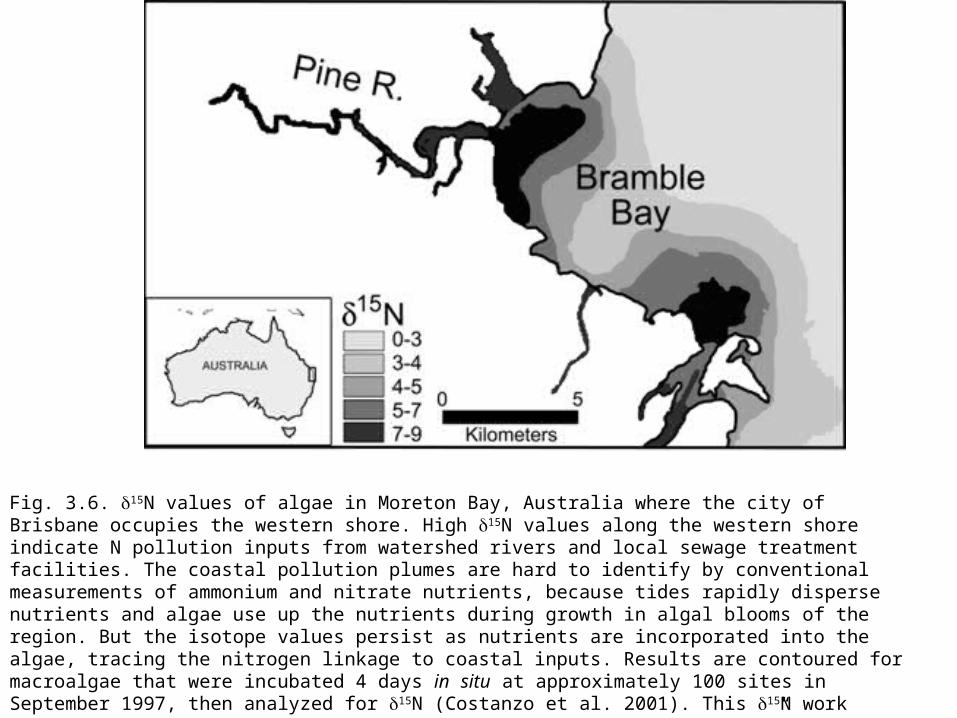
Fig. 3.6. 15N values of algae in Moreton Bay, Australia where the city of Brisbane occupies the western shore. High 15N values along the western shore indicate N pollution inputs from watershed rivers and local sewage treatment facilities. The coastal pollution plumes are hard to identify by conventional measurements of ammonium and nitrate nutrients, because tides rapidly disperse nutrients and algae use up the nutrients during growth in algal blooms of the region. But the isotope values persist as nutrients are incorporated into the algae, tracing the nitrogen linkage to coastal inputs. Results are contoured for macroalgae that were incubated 4 days in situ at approximately 100 sites in September 1997, then analyzed for 15N (Costanzo et al. 2001). This 15N work continues now as a monitoring technique termed “sewage plume mapping” (Costanzo et al. 2005). Reprinted from Marine Pollution Bulletin 42:149-156, S.D. Costanzo, M.J. O’Donohue, W.C. Dennison, N.R. Loneragan, and M. Thomas, A new approach for detecting and mapping sewage impacts. Copyright 2001, with permission from Elsevier.

Fig. 3.7. 13C values of soils from six sites in Gabon, Africa where C4 savannah grasses (-12o/oo) and forest trees (-29o/oo) contribute to soil organic matter. Low values near -29o/oo indicate landscapes dominated by forests, while high values approaching -12o/oo indicate landscape-level shifts to open savannah. The square symbols give the isotope values for forest soils in a reference undisturbed system that has not been invaded by savannah. Considering the isotope profiles of the other non-reference soils as a history and reading from the bottom up, forests dominated the landscape until about 3000 years ago when the landscape shifted to open savannah, but this trend reversed about 750 years ago, with forests now dominating again. From: Delegue, M.-A., M. Fuhr, D. Schwartz, A. Mariotti and R. Nasi. 2001. Recent origin of a large part of the forest cover in the Gabon coastal area based on stable carbon isotope data. Oecologia 129:106-113. This is reprint of Figure 2, p. 109 from the article and is used with permission from Springer.

Fig. 3.8Effects of species introductions measured in lake ecosystems. Introduction of nearshore bass species forces the native top predator, lake trout, offshore. Reflecting this spatial displacement, lake trout diets shift towards feeding in a more pelagic food web (as measured by lower 13C) and at a lower trophic level (as measured by lower15N; with 15N translated into the y-axis “trophic level” in this figure). Dietary shifts help explain the decline of lake trout in the invaded lakes. This figure summarizes results from comparative studies in different lakes and results for single lakes studied over time (from Vander Zanden et al. 1999; used with the permission of the author and Nature Publishing Group. Copyright 1999).

Fig. 3.9. Isotope map of North America for precipitation D values. Plant and animal D values reflect this continental-level map. The map is reprinted from Taylor, Jr., H.P., 1974, Economic Geology 69(6), p. 850, Fig. 6.

Fig. 3.10. D values of feathers collected from Wilson’s Warblers that overwintered at sites from central America (10o N) to the southern United States (35o N). Animals collected farthest south at 10oN had the lowest D values, so that their point of origin for the migration was in the far north (see previous Fig. 3.9). These long-distance migrators moved past and leap-frogged over other populations that move much less during their fall and winter migrations (From: Kelly, J.F., V. Atudorei, Z.D. Sharp and D.M. Finch. 2002. Insights into Wilson’s Warbler migration from analyses of hydrogen stable-isotope ratios. Oecologia 130:216-221. This is a reprint of Figure 6 on p. 219 of the article, used with permission from Springer).

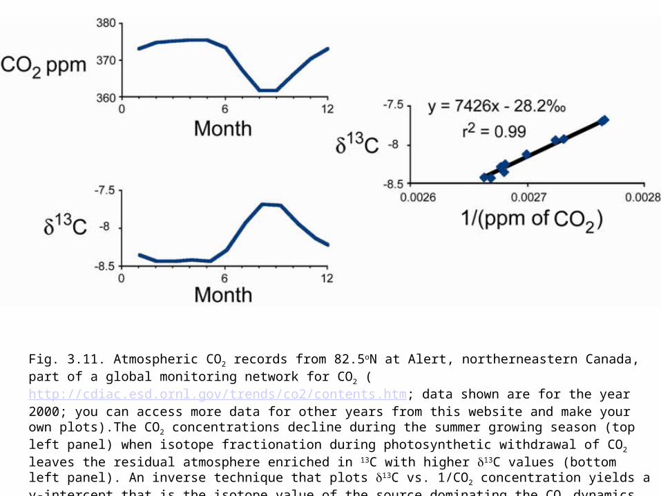
Fig. 3.11. Atmospheric CO2 records from 82.5oN at Alert, northerneastern Canada, part of a global monitoring network for CO2 (http://cdiac.esd.ornl.gov/trends/co2/contents.htm; data shown are for the year 2000; you can access more data for other years from this website and make your own plots).The CO2 concentrations decline during the summer growing season (top left panel) when isotope fractionation during photosynthetic withdrawal of CO2 leaves the residual atmosphere enriched in 13C with higher 13C values (bottom left panel). An inverse technique that plots 13C vs. 1/CO2 concentration yields a y-intercept that is the isotope value of the source dominating the CO 2 dynamics, in this case -28.2o/oo carbon from C3 plants (middle right panel).