Embed Size (px)
Citation preview

Filter Flow made Practical: Massively Parallel and Lock-Free
Sathya N. Ravi
University of Wisconsin-Madison
Yunyang Xiong
University of Wisconsin-Madison
Lopamudra Mukherjee
University of Wisconsin-Whitewater
Vikas Singh
University of Wisconsin-Madison
Abstract
This paper is inspired by a relatively recent work of
Seitz and Baker which introduced the so-called Filter Flow
model. Filter flow finds the transformation relating a pair
of (or multiple) images by identifying a large set of lo-
cal linear filters; imposing additional constraints on cer-
tain structural properties of these filters enables Filter Flow
to serve as a general “one stop” construction for a spec-
trum of problems in vision: from optical flow to defocus
to stereo to affine alignment. The idea is beautiful yet the
benefits are not borne out in practice because of signifi-
cant computational challenges. This issue makes most (if
not all) deployments for practical vision problems out of
reach. The key thrust of our work is to identify mathemat-
ically (near) equivalent reformulations of this model that
can eliminate this serious limitation. We demonstrate via a
detailed optimization-focused development that Filter Flow
can indeed be solved fairly efficiently for a wide range of in-
stantiations. We derive efficient algorithms, perform exten-
sive theoretical analysis focused on convergence and par-
allelization and show how results competitive with the state
of the art for many applications can be achieved with neg-
ligible application specific adjustments or post-processing.
The actual numerical scheme is easy to understand and, im-
plement (30 lines in Matlab) — this development will enable
Filter Flow to be a viable general solver and testbed for nu-
merous applications in the community, going forward.
1. Introduction
Understanding how two or more images of the same
scene are related, is a fundamental problem in computer vi-
sion. Often, the coordinate systems of the respective im-
ages are related by a camera motion whereas in other cases,
the scene illumination may change, the shading may dif-
fer and/or the exposure, zoom and other parameters of the
camera may be modified from one image to the other. These
effects typically lead to a systemic (but otherwise arbitrary)
transformation in the image intensities. To enable follow-up
analysis, an important first step is to recover the parameters
describing the relationship between the images.
While technically accurate, the above description actu-
ally covers a large class of problems with a broad stroke.
In practice, instead of a common strategy, most problems
in this class are addressed piecemeal, by posing it as a par-
ticular instantiation of the high-level “transformation esti-
mation” objective. One makes explicit use of additional in-
formation pertaining to the specific problem to be solved
(such as acquisition details, parameters to be estimated and
application specific constraints). The representative prob-
lems in this class correspond to a number of core topics in
modern vision literature: optical flow[30, 24, 38], decon-
volution [21, 27], non-rigid morphing [25], stereo (plus its
variations)[34, 23, 37], defocus [22] and so on — these are
all distinct problems but at the high level, deal with esti-
mating the relationship between two or more images. This
compartmentalized treatment has, over the years, provided
highly efficient algorithms and industry-strength implemen-
tations for numerous problems. Such solutions now drive
any number of downstream turnkey applications.
Despite this diversity of highly effective and mature al-
gorithms for each stand-alone problem, an interesting scien-
tific question is the following. Given that many of these for-
mulations seek to estimate a transformation which explains
the change in image intensities over two (or more) images,
can we design a unified formulation that is rich enough to
model a broad class of transformations and yet offers the
flexibility to precisely express the nuances of each distinct
problem listed above? In an interesting paper a few years
back, Seitz and Baker, provided precisely such a framework
called Filter Flow [35]. Filter Flow models image transfor-
mations as a to-be-estimated space-variant (pixel-specific)
13549

linear ‘filter’ relating a pair of images I1 and I2 as,
I2 = TI1, T ∈ Γ, (1)
where T can be thought of as a filter (or operator) whose
rows act separately on a vectorized version of the source im-
age I1. Observe that the inverse problem of computing the
transformation, T , specified by the first identity is severely
under constrained. For Model (1) to make sense, T ∈ Γmust serve as a placeholder for the entire set of additional
constraints on the filter which enables a unique solution that
satisfies our expectations for particular problems of inter-
est, e.g., optical flow, stereo with illumination change or
affine alignment. But imagine if the problem specific re-
quirements can actually be encoded as a feasibility set, Γ –
then – the Filter Flow formulation offers an interesting “one
stop” model where the unknown transformation we seek to
estimate is linear. It turns out that an entire catalog of vision
problems fit very nicely into this formulation: from defocus
to stereo with higher order priors to optical flow with rich
domain specific priors, each with its own specific feasibil-
ity set Γ. Such a formulation offers several advantages: (a)
it reparametrizes traditionally non-linear or variational for-
mulations into an optimization problem that may be solved
via just linear programming; (b) the form in (1) can be eas-
ily modified to incorporate additional domain specific pri-
ors which may alternatively need more significant structural
modifications in an algorithm designed for a particular ob-
jective and (c) while it may not be a silver bullet for all prob-
lems expressible in this form, the corresponding solutions
may provide a strong baseline and drive the development of
more efficient algorithms.
From a theoretical perspective, Model (1) is simple and
elegant. Unfortunately, a direct optimization of (1) is in-
tractable for image sizes we typically encounter in prac-
tice. Running the model in a medium to large scale set-
ting, e.g., for video sequences, is simply not possible. This
may seem counter intuitive, especially since the objective
and constraints are linear. So why is the model not solvable
by large scale linear programming solvers? It turns out that
while this approach guarantees global optimality, the con-
straint matrix arising from practical problem sizes, cannot
be instantiated, even on a high end workstation. Even when
multi-resolution pyramid schemes are adopted as a practi-
cal heuristic, the running times range from 9 to 20+ hours,
depending on the type of problem and the associated con-
straints, a weakness acknowledged by the authors [35]. Fur-
thermore, some problems require adding terms in the objec-
tive that are non-convex; these are solved via a series of lin-
ear programs (obtained using linear approximations at each
iteration). In summary, the potential scope and applicabil-
ity of this interesting formulation has not been fully real-
ized, in large part due to its serious computational footprint.
The main goal of this paper is to remove this limitation and
make Filter Flow practical.
Related Work: The main motivation of this paper is to
devise practical algorithms for Filter Flow [35]. In addi-
tion, we discuss several case studies in Section 5, specific
to problems which can be modeled as Filter Flow. The lit-
erature dealing with these problems such as Optical Flow
[18, 1], Affine Alignment [20] and Stereo matching[14, 17]
is quite mature and is not discussed at length here to avoid
digressing from the main algorithmic focus of the paper.
Before moving on, we point out that Fleet et al., [10] also
proposed linear motion models to represent varied or com-
plex motions and many of our constructions will be appli-
cable to the ideas in these earlier papers.
We highlight some application domains where the filter
flow model has been recently applied fairly successfully. In
[16], the authors proposed an approach which made the fil-
ter flow construction efficient for space-variant Multiframe
Blind Deconvolution. Later, [9] used this formulation for
computing scene depth from a stereo pair of cameras un-
der a sequence of illumination directions. Filter Flow has
been used effectively for fast removal of Non-uniform Cam-
era Shake and the resultant blurs in [15]. Others [32] have
reformulated the smoothness prior in Filter Flow, to make
it suitable in various applications including alpha matting.
These methods demonstrate that the applicability of Filter
Flow to a set of diverse problems is possible but has of-
ten involved disparate solution schemes. We believe that
once the computational challenges are resolved, filter flow
approaches will be more widely adopted in vision.
Contributions. Our earlier discussion suggests that
commercial Linear Programming (LP) solvers are not well
suited for solving (1). However, we find that in most in-
stantiations of Filter Flow (in the context of specific vision
problems), the problem has significant structure that can be
exploited via specialized optimization schemes. In partic-
ular, we see that for each of the five case studies cover-
ing problems such as affine alignment and optical flow de-
scribed in [35], a nearly equivalent reformulation allows the
applicability of numerical optimization schemes that cuts
down the running time from tens of hours to several min-
utes on a standard workstation, without making use of any
heuristic strategies. By nearly equivalent, we mean that the
problems have the same optimal solution up to chosen tol-
erance. On the modeling side, we propose a new convex
term that encourages sparsity which is called the compact-
ness term, an ℓ2 data term and a valid inequality that re-
duces the search space of the parameters. On the algorith-
mic side, with some more manipulation, the problems re-
veal additional structure appropriate for massively parallel
lock-free implementations. To that end, we propose an ef-
ficient asynchronous parallel algorithm that solves our for-
mulation 30 times faster than the previous model and are
empirically competitive to the state of the art solvers both
3550

quantitatively and quantitatively. A detailed description of
these properties and the corresponding algorithms with con-
vergence guarantees is our main contribution.
Notations: We use ei’s to represent the standard basis
vectors and 1 denotes the vector of all 1’s. Also, ∆ gives
the probability simplex in appropriate dimensions. Small
alphabets represent vectors over R; upper-case letters rep-
resent linear maps between vector spaces over R. All proofs
are included in the appendix due to space constraints.
2. A brief overview of Filter Flow
We briefly review the key components of Filter Flow [35]
to set up our discussion. Let I1 and I2 be a pair of images
for which Filter Flow is to be computed. In our formulation,
I1 and I2 can be assumed to be vectors in Rn, where n is the
total number of pixels in image I1 (or I2). Then filter flow
can be formulated as the following optimization problem1,
minT∈Rn×n
||TI1 − I2||22. (2)
Equivalently, the ith entry of TI1 is the linear combina-
tion of intensities of I1. The authors in [35] further decom-
pose T as T = MK where M is a motion matrix and Kis a kernel matrix. M−1 encodes the motion from I2 to I1,
so we can write the objective as ||MI2 − KI1||22. In par-
ticular, in the case of pure motion, K is the identity matrix.
Our construction can be employed for a nontrivial K but we
assume that K is the identity matrix to simplify our presen-
tation and without loss of generality swap I2 and I1. Since
this formulation is under constrained, [35] proposes some
natural constraints on M , described below.
Non-Negativity: Negative coefficients are meaningless;
so one imposes the constraint that M ≥ 0.
Row Simplex Constraint: We also require that, the sum
of coefficients in each row of M to be 1, i.e., each pixel in
I2 is a convex combination of pixels in I1. In addition, we
define a neighborhood of each pixel i as N (i) and ensure
that pixels outside this neighborhood do not participate in
the convex combination. Hence, we can write the optimiza-
tion problem that we seek to solve as,
minM≥0
||MI1 − I2||22 (3)
s.t.∑
j∈N (i)Mij = 1,∑
j 6∈N (i)
Mij = 0, ∀i = 1 to n.
While the above description serves as the basic template of
the Filter Flow model, various additional constraints and
terms are added in problem (3) to model the underlying
computer vision problem of interest. Specific examples in-
clude: (i) for the Affine alignment problem, the requirement
1Via personal communication [35], we know that the norm was chosen
to allow applicability of LP solvers and not central to the model otherwise.
that all pixels in I1 are transformed by an affine matrix A(the so-called GLOBA-M constraints in [35]); (ii) for op-
tical flow, we encourage smoothness on the affine motion
of neighboring pixels; (iii) for precise integer flow, terms
encouraging sparsity are introduced; (iv) for stereo, we re-
quire smoothness between the rows of M . Specific details
of these terms will be described later in case studies.
3. Algorithmic Reformulations
Our basic hypothesis is that reformulating the filter flow
problem will enable us to design practical algorithms with
global convergence guarantees. Unfortunately, additional
terms/constraints (described in the previous section) that are
used in specific formulations of standard computer vision
problems, make this task non-trivial. The reason is two-
fold: (i) non-convexity in some of the decision variables
and, (ii) even when the optimization problem is convex, the
additional terms lead to composite functions or constraints.
For example, in imposing affine smoothness (used in op-
tical flow), we add the term∑
i
∑
j∈N (i) ||Ai − Aj ||22 in
the objective, where Ai is the affine motion associated with
pixel i. Such terms make it hard to optimize the problem
using standard off the shelf solvers, since it requires multi-
ple passes over the data to compute the gradient. Our goal
with the reformulations is to mitigate such issues while also
preserving the overall behavior of the filter flow model.
Next, we will identify a few high-level issues that make
the optimization challenging for the constraints mentioned
in [35] and offer alternatives. Our line of attack (or work-
flow) is as follows. We will first address the main (compu-
tationally) problematic pieces of the Filter Flow model and
provide tractable reformulations for each. Our hope will be
that these reformulations will satisfy “nicer” technical con-
ditions that will guide the choice of the overall optimiza-
tion scheme. We will then describe how this scheme can
be further specialized by exploiting the problem structure
for particular computer vision problems (case studies). The
objective will be that each specific instantiation should be
implementable just by modifying a few lines of code of the
overall optimization and still preserve efficiency benefits.
3.1. Reformulating Compactness
Ideally, we want to find a correspondence between the
pair of images where each pixel in I1 is mapped exactly
to a single pixel in I2. To ensure sparsity, [35] proposed a
compactness term, defined as,
∑
i
∑
j∈N (i)
Mij ||(j − i)−∑
ij
Mij(j − i)||22 (4)
But the compactness term makes the objective function
nonconvex (in fact, concave), therefore, a linearization ap-
proach had to be used in [35]. Initially the compactness
3551

term is set to zero and the optical flow is computed with-
out the compactness term. After the first iteration, a linear
approximation of the compactness function is used and the
corresponding linear program (LP) is solved. This requires
solving a huge LP problem multiple times (even though em-
pirically the number of iterations used was only 3−4). Sec-
ondly, the solver needs to do a full pass of the data (or im-
age) in order to compute the linear approximation of com-
pactness, which is expensive.
A Convex Compactness term? To successfully replace
the compactness term with a more efficient substitute, we
first consider some useful properties that such a term needs
to encode: 1) as the regularization parameter increases, it
should tend towards keeping a single non-zero entry in each
row, 2) the value of the function and its derivative should be
efficiently computable and, 3) it should be easy to optimize.
To this end, the ℓ1 norm is a natural choice to get sparse
solutions. But it turns out that the ℓ1 norm is constant (= 1)
on the feasible set of our problem, so it is not applicable.
However, observe that the constraints on the matrix M im-
ply that M is a row stochastic matrix. So, if we consider
each row of M to be a probability distribution on n vari-
ables, then we need the optimal probability distribution to
have small support, that is, we want our compactness term
to behave like a linear combination of the fewest number
of delta functions. In [28], the authors showed that a re-
laxed version of this problem can be solved by n second
order cone programs in parallel. Later, [8] provided a con-
vex formulation that encourages sparsity on the simplex and
showed that it is more robust. Using these ideas which are
demonstrated empirically in the appendix, we can write our
problem as,
minM≥0
||MI1 − I2||22 + λ1
n∑
i=1
||M[:,i]||2 (5)
s.t.∑
j∈N (i)
Mij = 1,∑
j 6∈N (i)
Mij = 0, ∀ i
where λ1 > 0 is fixed and M[:,i] denotes the i−the column
of M and λ1 is the regularization parameter. Intuitively,
the penalty is a group lasso type penalty with the groups
given by the columns of M . Therefore, this term encour-
ages that there are few nonzero entries along the columns
and together with the sum to one constraint on the rows
makes the rows sparse, achieving the desired property.
3.2. Reformulating Affine Smoothness
Ensuring smoothness of the transformation across the
pixels is important for several problems such as Optical
Flow. Affine smoothness terms, in such instances were
shown in [35] to outperform other second order smooth-
ness terms and yield a smoother flow field in practice. To
encourage affine smoothness, we define an explicit 6 pa-
rameter affine transformation at each pixel i, denoted by
Ai ∈ R2×3. Intuitively, Ai captures the motion of the cen-
troid of the filter at pixel i. To do so, [35] imposes a hard
“LOCA-M” constraint (set the flow equal to the centroid).
Instead, we use the dual form and add the terms in the ob-
jective function (λ2 > 0), that is,
λ2
∑
i
||Aii− Mi||22 (6)
where Mi ∈ R2 is the centroid of filter at pixel i and i ∈ R
3
is the pixel i in homogeneous coordinates with third entry
equal to 1. We fix the value of λ2 whenever approximate so-
lutions are enough. We treat them as a quadratic penalty if
more accurate solutions are required which guarantees (see
[26]) that the equality constraint is satisfied when our algo-
rithm terminates, exactly as desired in [35]. Finally, to get
a smooth flow, the following term is added to the objective
function (λ3 > 0),
λ3
∑
i
∑
j∈N (i)
||Ai −Aj ||22 (7)
Now, we give a result showing an interesting property of
the affine transformation matrix and is relevant in informing
the choice of algorithm in the next section.
Lemma 3.1 ||Ai||2F ≤ C is a valid inequality for a suffi-
ciently large C > 0.
Intuitively, this lemma says that the magnitude of each
individual element of Ai’s is bounded (with C chosen ap-
propriately). Observe that i ≥ 1 (coordinatewise) and the
restriction of the movement of a pixel to be within the filter
implies that Mi is bounded by the neighborhood size giving
us the tightest choice for C. This lemma implies that (one
of) the optimal solution(s) of the least squares problem is
contained in a convex compact set. More importantly, this
lemma shows that we have not compromised any theoretical
property by adding this inequality.
3.3. Which solver should we use?
One of the key differences between the model in [35]
and our approach is that the we replaced the ℓ1 norm with
special type of compactness encouraging norm making the
objective a smooth convex function. In this section, we will
see how this change of norm together with the above lemma
enables leveraging recently developed convex optimization
techniques that can speed up the optimization time by sev-
eral orders of magnitude, assuming that the case study spe-
cific terms can also be manipulated and reformulated to be
amenable to our optimization scheme.
We now discuss how two key properties viz., approxima-
tion and randomization will guide the choice of an appro-
priate optimization scheme. We motivate these choices next
in the context of our model.
3552
A) Approximation: Consider the problem of solving
a finite dimensional optimization problem over a compact
convex set. Such problems are often solved using projected
gradient methods (over multiple iterations), which involves
projection of the objective at each step on the feasible set.
This requires optimizing a quadratic function on the feasible
set. These algorithms allow large changes in the working
set at each iteration unlike active-set methods and therefore
can be applied to large size problems. The primary disad-
vantage, however, is that even when the feasible set is very
simple such as probability simplex, ellipsoids, ℓ1 norm ball,
the corresponding projection subproblem is nontrivial. On
the other hand, there are constrained optimization methods
that consist of optimizing a linear function over the feasible
set at each iteration. In the literature, methods which solve
problems of the above form are referred to as feasible direc-
tions method [3]. Specifically, Conditional Gradient Meth-
ods (CGM) is a class of feasible directions method which
has been shown to have better theoretical convergence rates
[3] and is applicable to our Filter Flow model. Recently,
CGMs have performed well in solving many machine learn-
ing problems including SVMs and nuclear norm regular-
ized problems, see [12, 19] though have only been sparingly
used in vision. Indeed, the method thrives in practice when
the following two properties are satisfied: i) feasible set is
compact convex; and ii) optimizing a linear function over
the feasible set is easy.
B) Randomization: As mentioned earlier, the double
summation terms in (7) is a computational bottleneck, since
it needs to make a full pass over the data to compute the gra-
dient. It has been shown [2, 29] that approximate first order
information can be used to solve such large scale optimiza-
tion problems, referred to as randomized or stochastic algo-
rithms. These methods are much faster than the traditional
algorithms and are often provably robust to noise [13].
Our strategy is to combine Conditional Gradient meth-
ods with randomization to develop efficient Randomized
Block Coordinate Conditional Gradient [6, 5] algorithm
(RBC-CGM) with strong sparsity and convergence guaran-
tees to solve standard Filter Flow formulations. We show
how RBC-CGMs can be efficiently used in tandem with
powerful distributed convex optimization schemes result-
ing in practical algorithms for these problems. Before we
present the randomized version, we briefly review the (de-
Algorithm 1 Conditional Gradient Method (CGM)
Pick a starting point x0 ∈ C.
for t = 0, 1, 2, · · · , T do
g ← ∇f(xt)s← argmins∈C s
tg (*)xt+1 ← (1− γt)xt + γts
end for
terministic) Conditional Gradient Method.
Conditional Gradient Method (CGM): CGM solves
problems of the form, minx∈C f(x), where f is a finite di-
mensional smooth convex function and C is compact con-
vex set. Given a feasible starting point, each iteration of
the algorithm solves a linear approximation of f over C and
chooses a point in the line segment joining the current point
and the solution to the linear approximation. This makes
sure that the new point is also feasible. The basic algorithm
for CGM is shown in Alg. 1.
Assuming that the gradient can be computed easily, step
(*) in Algorithm 1 determines the complexity of CGM. Ob-
serve that the requirement of C to be bounded is necessary
since otherwise s from step (*) will be unbounded. CGM
finds the global optimal solution of the reformulated Filter
Flow problem since M is bounded by construction in (5),
and Ai’s are bounded by lemma (3.1). This suggests that
if we temporarily do not worry about the problem specific
reformulations, CGM can be deployed easily.
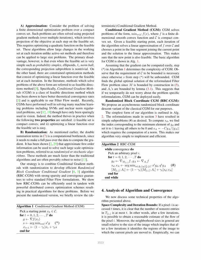
Randomized Block Coordinate CGM (RBC-CGM):
We propose an asynchronous randomized block coordinate
descent variant of the classical CGM for our purposes.
The simplest form of our algorithm is outlined in Alg.
2. The reformulations made in section 3 have resulted in
simple subproblems (#) as desired. To compute sd, we find
the index corresponding to the minimum element of gd and
set it to 1 leaving all others to be 0 and sA = −CgA/||gA||which requires the computation of a norm. This makes our
algorithm very simple to implement and efficient.
Algorithm 2 RBC-CGM
while convergence do
Pick an arbitrary pixel i.for t = 0, 1, 2, · · · , T do
gd ← ∇M[i,:]f , gA ← ∇Ai
f
sd, sA ← argmins∈∆,||q||2F≤C stgd, q
tgA (#)[M[i,:];Ai]← (1− γt)[M[i,:];Ai] + γt[sd; sA]
end for
end while
4. Analysis of Algorithm and Convergence
We now discuss some technical properties of the algo-
rithm presented above.
Space Complexity and Iteration Bounds: If a pixel i is ac-
cessed t times, it is clear that the number of nonzero entries
in T[i,:] is at most t. In other words, after a few iterations,
it is possible to obtain a reasonable estimate of the flow of
the pixel i. Moreover, the neighborhood sizes in general are
small relative to the size of the image which implies that af-
ter a few iterations it identifies the regions of the image to
which the current pixels are moved to. Empirically, we can
3553

stop after 100 epochs, (i.e., when each pixel is accessed 100
times by the processor) if the filter size is [−10, 10]2. Sec-
ond, we can easily estimate the number of iterations needed
before starting the algorithm for a fixed amount of memory.
We will now prove a lemma (proof in appendix) that es-
tablishes a block-descent property for this algorithm which
can be used to trivially parallelize the algorithm.
Lemma 4.1 Denote the objective as f(y) : Rn → R where
f is convex, smooth and that y is partitioned into J ={1, ..., J} blocks, i.e., y = [y1, y2, ..., yJ ] such that yi ∈ Yj ,
then we have that dTi ∇if(yi(t)) ≤ −C ′||di(t)||22, where di
is the direction of update i.e., yi(t + 1) = yi(t) + γtdi(t)and C ′ > 0 is a constant.
Parallelization: Using the above lemma and proposition 5.1
in [4], we can deploy an asynchronous algorithm assum-
ing that the time delay between the updates of processors is
bounded. Of course, this does not prove that each update
decreases the objective function maintaining feasibility. In
fact, this is rarely true in conditional gradient type meth-
ods except if we use line search methods to compute step
sizes γt that satisfy Armijo condition. But this defeats the
purpose of asynchronous methods because each processor
will take arbitrarily long to do a single update thus affect-
ing the convergence rate. Moreover, constant step size poli-
cies usually depend on parameters of the objective function
and constraints that are hard to compute a priori. Fortu-
nately, in the convergence proofs of this method, we show
that a particular choice of stepsize sequence determined a
priori guarantees convergence (see [19]) and only depends
on the iteration number making the algorithm naturally easy
to parallelize [4]. It is useful to see that the convergence is
established using the duality gap principle and not just using
the primal optimization problem. The above lemma shows
the correctness of our algorithm, that is, any limit point of
the sequence generated by our algorithm converges to the
optimal solution at the rate equal to its sequential version,
that is, O(1/√N). For explicit convergence rates, see [36].
Many aspects that are considered in [36] like collisions, de-
layed updates do not affect the problems considered here
since the delay between individual workers is negligible.
So, our proof is much simpler. We will now see how the
update schemes change for specific problems.
5. Case Studies
We study three specific problems, that immediately benefit
from the fast filter flow formulation. We also discuss paral-
lel solvers, if applicable.
Affine Alignment: The Affine Alignment problem deals
with the task of finding global affine alignment between a
pair of images. It can be formulated as
minM,A||MI1 − I2||22
s.t. M [i, :] ∈ ∆, ||A||2F ≤ C,Ai = Mi ∀i(8)
where A ∈ R2×3 is the global affine matrix capturing the
affine warp between I1 and I2 and ∆ is the unit simplex.
Let Ai be the affine matrix for each pixel i. Then, we can
write an equivalent form of (8) as,
minM,A||MI1 − I2||22
s.t. M [i, :] ∈ ∆,Aii = Mi, Ai = A, ||Ai||2F ≤ C ∀i(9)
After dualizing the equality constraints Ai = A, we can
write the optimization problem as (λ > 0),
minM,A||MI1 − I2||22 + λ
∑
i
||Ai −A||2F
s.t. M [i, :] ∈ ∆, Aii = Mi, ||Ai||2F ≤ C ∀i(10)
Note that this problem satisfies the two properties men-
tioned in section 3.3.
Parallelization: The model (10) can be easily parallelized
as follows. Each worker picks a pixel i, solves the corre-
sponding optimization problem and updates Ai. Observe
that we do not explicitly impose that ||A||2F ≤ C in the
model. After all the workers update Ai, A can be updated
as,
A← argminA
∑
i
||Ai −A||2F (11)
But the above optimization problem simply computes the
mean of all Ai’s which can be done in time linear in the
number of pixels. We use incremental gradient descent
method with 0 < α < 1 as the dual step size to update
λ, see [2], λ← λ+ α · (∑i ||Ai −A||2F ).Optical Flow: Putting together the objective and con-
straints from Section (3) pertaining to optical flow, we can
write the optimization problem as follows:
minM≥0,Ai
||MI1 − I2||22 + λ1
n∑
i=1
||M[:,i]||2
+∑
i
λi2||Aii− Mi||
22 + λ3
∑
i
∑
j∈N (i)
||Ai −Aj ||22
s.t.∑
j∈N (i)
Mij = 1,∑
j 6∈N (i)
Mij = 0, ||Ai||2F ≤ C ∀i
(12)
Note that λ1 and λ3 are parameters for the optimization
problem, therefore user specified constants. The main dif-
ference in this model from the affine alignment problem is
that we use a different dual variable λi2 for each pixel. This
is often useful since optical flow is computed using a pyra-
mid approach, so we get a good initialization of Ai’s locally.
Again, we see that this problem satisfies the two properties
3554

Figure 1: Optical flow results: The first 4 columns shows results on the MPI Sintel dataset, the last 4 columns show results on the Middlebury dataset.
Columns 1 to 3 (5 to 7) show the ground truth, our result and the Epicflow result respectively. Column 4 (and 8) shows the error map. AEE’s of column 4
are 1.08, 1.15, 1.03 for rows 1 to 3. AEE’s for column 8 are 0.06, 0.042, 0.033 for rows 1 to 3. Our results are marked in red.
mentioned in section 3.3.
Parallelization: Each worker solves the following problem,
minM[i,:],Ai
(M t[i,:]I1 − etiI2)
2 + λi2||Aii− Mi||22
+∑
j∈N (i)
||Ai −Aj ||22 + λ1
n∑
i=1
||M[:,i]||2
s.t. M[i,:] ∈ ∆, ||Ai||2F ≤ C
(13)
The optimization problems and the λi2 can be updated and
stored locally in each worker. This gives us a lock free asyn-
chronous parallel algorithm. After each worker finishes the
above subproblem, λi2 are updated as,
λi2 ← λi
2 + α ·(
||Aii− Mi||22)
(14)
Stereo: Stereo matching problem is formulated using a
local smoothness model instead of global affine smoothness
as follows:
minM≥0
||MI1 − I2||22 + λ1
n∑
i=1
||M[:,i]||2 + λ3
∑
i,j
||Mi −Mj ||22
s.t.∑
j∈N (i)
Mij = 1,∑
j 6∈N (i)
Mij = 0, ∀i (15)
Updates here are a special case of updates for the optical
flow problem, so the same parallelization scheme applies.
6. Experiments
We present experimental results on three case studies in-
troduced in Section 5. Our goal is to evaluate (a) the de-
gree of runtime improvements of our algorithm over alter-
natives which uses no reformulation strategies; (b) whether
the reformulated Filter Flow model when solved to opti-
mality can, in fact, yield results competitive with dedicated
algorithms developed specifically for each case study; and
(c) whether the overall scheme is efficient enough to enable
rapid prototyping for new problems in vision that fit into the
model in (3). We discuss these issues next.
Setup: First, we briefly describe the experimental setup.
Initialization: We use the Lucas Kanade algorithm to get an
initial estimate of the flow, which works for most settings.
Step Size: The choice of the stepsize γt determines con-
vergence. While line search can be used, it may be sub-
optimal for the (partially) asynchronous aspect of our algo-
rithm (e.g., time delay between processors). For our paral-
lelized version, each processor uses its own iterations count.
We use the strategy proposed in [11] by setting γt =2
κ+t+2where κ > 0 is a constant that depends on the objective.
Implementation: We used a 8-core 3.60GHz processor ma-
chine with 12GB RAM, and Intel TBB within C++ for task
parallelism. We fix λ3 = 0.005, λ1, λ2 = 1 for all problems
and all datasets. No other parameter tuning was performed.
Note that evaluating Filter Flow[35] on high resolution
images is problematic because of the cost of solving the
corresponding LP. Therefore, we use a state of the art op-
tical flow method [31] for comparison. For low resolution
images, the results of our method and Filter Flow were qual-
itatively and quantitatively similar (see Appendix).
Optical Flow: We start with the Optical Flow problem
since from a Filter Flow perspective, it is computationally
the most demanding [35]. We used two standard optical
flow datasets: MPI Sintel [7] and Middlebury [1]. MPI Sin-
tel is a large displacement dataset whereas Middlebury has
more nonlinear movements. MPI Sintel consists of two ver-
sions of sequences, clean and final with the same ground
truth. To show the performance (both qualitative and run-
time) of the “standard” Filter Flow formulation in [35], the
model was not augmented with additional constraints to
handle occlusion, blur and lighting effects explicitly. There-
Method Final pass Clean pass
all noc occ d0-10 s10-s40 all noc occ d0-10 s10-s40
F3-MPLF (Ours) 6.272 3.092 32.207 5.042 3.226 4.770 2.062 26.863 3.459 1.883
FlowFields 5.810 2.621 31.799 4.851 3.739 3.748 1.056 25.700 2.784 2.110
FullFlow 5.895 2.838 30.793 4.905 3.373 3.601 1.296 22.424 2.944 2.055
DiscreteFlow 6.077 2.937 31.685 5.106 3.832 3.567 1.108 23.626 3.398 2.277
EpicFlow 6.285 3.060 32.564 5.205 3.727 4.115 1.360 26.595 3.660 2.117
TF+OFM 6.727 3.388 33.929 5.544 3.765 4.917 1.874 29.735 3.676 2.349
NNF-Local 7.249 2.973 42.088 4.896 4.183 5.386 1.397 37.896 2.722 2.245
Figure 2: Optical flow results on the test set of MPI Sintel dataset.
3555

· · ·
Figure 3: Stereo results: (From left to right) First three plots show the evaluation on Middlebury 2011 dataset. Our results match the ground truth closely;
the last three show the evaluation on Recycle pair from 2014 Middlebury dataset; the fifth image is the result after 10% of total epochs whereas the last
image is the result after 50%. This implies that running more epochs progressively gives more accurate solutions. Our results are marked in red.
fore, we report results for our method and Epicflow [31] on
the clean sequences (note that additional terms within Γ can
incorporate these case specific constraints).
Representative qualitative results are shown in Fig. 1 for
MPI Sintel and Middlebury datasets. Results on the test
set of MPI Sintel is shown in Fig. 2. The results in Fig.
1 strongly suggest that qualitatively, our results are clearly
comparable to those obtained from Epicflow. In MPI Sintel
(Fig. 1 (top row)), our results show better consistency with
the ground truth (wedge on the left, small flows in the hair
region). The error discrepancy map in column 4 is nearly all
black. In Fig. 1 (row 2), our solution is able to accurately
recover the flow in the yellow region although the estima-
tion in the head region is more blurred. In Fig. 1 (row
3), the results from both methods are identical. The Av-
erage Endpoint Error (AEE), calculated as Frobenius norm
over the number of pixels, was in the range [0.03, 0.06] and
[1.02, 1.2] for Middlebury and MPI Sintel datasets respec-
tively for the non-occluded pixels. Quantitatively, this is
competitive with recent optical flow papers, that report re-
sults on these datasets. In most other sequences, we see a
similar overall behavior where our solution has good consis-
tency with the ground truth. This is particularly encourag-
ing because other than the constraints described in Section
5, no other optical-flow specific modifications were used.
No post-processing other than a median filter was needed.
Stereo: The main difference of the Stereo model from Opti-
cal Flow, is that it does not include the MRF-A terms, mak-
ing the optimization easier. We tested our algorithm on the
Middlebury Stereo 2014 [33] and 2011[1] datasets which
are standard stereo matching datasets. The 2014 dataset is
challenging because it includes 2864 × 1924 images with
large movements. Fig.3 shows representative results from
our algorithm. Our method does very well in finding the
correct matchings for the 2011 dataset with an overall AEE
of just 0.07. The 2014 dataset involves more iterations to
solve because of the size of the datasets, but the results are
comparable to those obtained from other methods.
Affine Alignment: Recall that an affine warp is completely
determined by 6 parameters. To test our algorithm, simi-
lar to [35], we artificially warped an image with an affine
transformation and then analyzed the error between the re-
covered A∗ and true A. Results show that the quantity
||A∗ − A||22 was very small (within 10−3) suggesting that
the recovered warp from the Filter Flow model is close to
the true warp. Our numerical scheme roughly takes ≈ 2minutes to solve, compared to≈ 3 hours mentioned in [35].
Overall, results presented here for 3 case studies show that
our Filter Flow solver provides high quality solutions to var-
ious image transformation problems. Additional results for
these case studies are in the Appendix.
Running Time Finally, we describe how our algorithm per-
forms w.r.t. to running time, which is arguably its most
significant strength. For all experiments, we ran only 150epochs of our algorithm: the sequential version of our al-
gorithm takes≈ 2 hours, whereas, our parallel implementa-
tion takes≈ 10 minutes for a 640×480 image pair showing
that the parallelized algorithm nearly gets a speedup propor-
tional to #cores. The appendix includes a plot for the con-
vergence of the objective function as directly suggested by
the theory. It gives empirical evidence that 150 epochs are
enough to get an approximate solution. Note that the cor-
responding times reported by Filter Flow [35] is 9+ hours.
7. Conclusions
We propose a reformulation of Filter Flow[35], which
makes it amenable to massively parallel asynchronous op-
timization schemes. Our reformulation is applicable to any
problem expressible in the Filter Flow format. The gen-
erality does not involve any practical compromise — we
show a range of experimental results demonstrating that
a mostly application-agnostic numerical solver can obtain
results that are competitive with specialized state of the art
techniques. Compared to the original model [35], the run-
time reduces from several hours to a few minutes. Interest-
ingly, the overall scheme is easy to implement and teach.
A prototype version of our solver is only about 30 lines of
Matlab code (see Appendix). The fully asynchronous solver
will be made available as a fork of OpenCV.
Acknowledgements This work is supported by NIH R01
AG040396 (VS), NSF CAREER RI 1252725 (VS), NSF
CCF 1320755 (VS), NSF CGV 1219016 (LM) and UW
CPCP (U54 AI117924). We thank Steven Seitz for numer-
ous discussions related to this work and also for contribut-
ing code. The code and the appendix is publicly available
at https://github.com/sravi-uwmadison/fast filter flow.
3556

References
[1] S. Baker, D. Scharstein, J. Lewis, S. Roth, M. J. Black, and
R. Szeliski. A database and evaluation methodology for opti-
cal flow. International Journal of Computer Vision, 92(1):1–
31, 2011. 2, 7, 8
[2] D. P. Bertsekas. Incremental gradient, subgradient, and prox-
imal methods for convex optimization: A survey. Optimiza-
tion for Machine Learning, 2010:1–38. 5, 6
[3] D. P. Bertsekas. Nonlinear programming. 1999. 5
[4] D. P. Bertsekas and J. N. Tsitsiklis. Parallel and distributed
computation: numerical methods, volume 23. 6
[5] T. Bonesky, K. Bredies, D. A. Lorenz, and P. Maass. A
generalized conditional gradient method for nonlinear oper-
ator equations with sparsity constraints. Inverse Problems,
23(5):2041, 2007. 5
[6] K. Bredies, D. A. Lorenz, and P. Maass. A generalized con-
ditional gradient method and its connection to an iterative
shrinkage method. Computational Optimization and Appli-
cations, 42(2):173–193, 2009. 5
[7] D. J. Butler, J. Wulff, G. B. Stanley, and M. J. Black. A nat-
uralistic open source movie for optical flow evaluation. In
A. Fitzgibbon et al. (Eds.), editor, European Conf. on Com-
puter Vision (ECCV), Part IV, LNCS 7577, pages 611–625.
Springer-Verlag, Oct. 2012. 7
[8] F. P. Carli, L. Ning, and T. T. Georgiou. Convex clustering
via optimal mass transport. arXiv preprint arXiv:1307.5459,
2013. 4
[9] H. Du, D. B. Goldman, and S. M. Seitz. Binocular photo-
metric stereo. In BMVC, pages 1–11. Citeseer, 2011. 2
[10] D. J. Fleet, M. J. Black, Y. Yacoob, and A. D. Jepson. Design
and use of linear models for image motion analysis. Inter-
national Journal of Computer Vision, 36(3):171–193, 2000.
2
[11] R. M. Freund and P. Grigas. New analysis and results for the
conditional gradient method. 2013. 7
[12] Z. Harchaoui, A. Juditsky, and A. Nemirovski. Conditional
gradient algorithms for norm-regularized smooth convex op-
timization. Mathematical Programming, pages 1–38, 2014.
5
[13] M. Hardt, B. Recht, and Y. Singer. Train faster, general-
ize better: Stability of stochastic gradient descent. arXiv
preprint arXiv:1509.01240, 2015. 5
[14] Y. S. Heo, K. M. Lee, and S. U. Lee. Illumination and camera
invariant stereo matching. In Computer Vision and Pattern
Recognition, 2008. CVPR 2008. IEEE Conference on, pages
1–8. IEEE, 2008. 2
[15] M. Hirsch, C. J. Schuler, S. Harmeling, and B. Scholkopf.
Fast removal of non-uniform camera shake. In Computer Vi-
sion (ICCV), 2011 IEEE International Conference on, pages
463–470. IEEE, 2011. 2
[16] M. Hirsch, S. Sra, B. Scholkopf, and S. Harmeling. Efficient
filter flow for space-variant multiframe blind deconvolution.
2010. 2
[17] H. Hirschmuller and D. Scharstein. Evaluation of stereo
matching costs on images with radiometric differences. Pat-
tern Analysis and Machine Intelligence, IEEE Transactions
on, 31(9):1582–1599, 2009. 2
[18] B. K. Horn and B. G. Schunck. Determining optical flow.
In 1981 Technical symposium east, pages 319–331. Interna-
tional Society for Optics and Photonics, 1981. 2
[19] M. Jaggi. Revisiting frank-wolfe: Projection-free sparse con-
vex optimization. In Proceedings of the 30th International
Conference on Machine Learning (ICML-13), pages 427–
435, 2013. 5, 6
[20] S. Lazebnik, C. Schmid, and J. Ponce. Semi-local affine parts
for object recognition. In British Machine Vision Confer-
ence (BMVC’04), pages 779–788. The British Machine Vi-
sion Association (BMVA), 2004. 2
[21] A. Levin, Y. Weiss, F. Durand, and W. T. Freeman. Un-
derstanding and evaluating blind deconvolution algorithms.
In Computer Vision and Pattern Recognition, 2009. CVPR
2009. IEEE Conference on, pages 1964–1971. IEEE, 2009.
1
[22] C. Li, S. Su, Y. Matsushita, K. Zhou, and S. Lin. Bayesian
depth-from-defocus with shading constraints. In Proceed-
ings of the IEEE Conference on Computer Vision and Pattern
Recognition, pages 217–224, 2013. 1
[23] X. Mei, X. Sun, W. Dong, H. Wang, and X. Zhang. Segment-
tree based cost aggregation for stereo matching. In Proceed-
ings of the IEEE Conference on Computer Vision and Pattern
Recognition, pages 313–320, 2013. 1
[24] M. Menze, C. Heipke, and A. Geiger. Discrete optimization
for optical flow. In German Conference on Pattern Recogni-
tion, pages 16–28. Springer, 2015. 1
[25] R. A. Newcombe, D. Fox, and S. M. Seitz. Dynamicfusion:
Reconstruction and tracking of non-rigid scenes in real-time.
In Proceedings of the IEEE conference on computer vision
and pattern recognition, pages 343–352, 2015. 1
[26] J. Nocedal and S. J. Wright. Numerical Optimization.
Springer, New York, 2nd edition, 2006. 4
[27] D. Perrone and P. Favaro. A clearer picture of total variation
blind deconvolution. IEEE transactions on pattern analysis
and machine intelligence, 38(6):1041–1055, 2016. 1
[28] M. Pilanci, L. E. Ghaoui, and V. Chandrasekaran. Recovery
of sparse probability measures via convex programming. In
Advances in Neural Information Processing Systems, pages
2420–2428, 2012. 4
[29] B. Recht, C. Re, S. Wright, and F. Niu. Hogwild: A lock-
free approach to parallelizing stochastic gradient descent. In
Advances in Neural Information Processing Systems, pages
693–701, 2011. 5
[30] J. Revaud, P. Weinzaepfel, Z. Harchaoui, and C. Schmid.
Epicflow: Edge-preserving interpolation of correspondences
for optical flow. In Proceedings of the IEEE Conference
on Computer Vision and Pattern Recognition, pages 1164–
1172, 2015. 1
[31] J. Revaud, P. Weinzaepfel, Z. Harchaoui, and C. Schmid.
EpicFlow: Edge-Preserving Interpolation of Correspon-
dences for Optical Flow. In CVPR 2015 - IEEE Conference
on Computer Vision & Pattern Recognition, 2015. 7, 8
[32] C. Rhemann, C. Rother, P. Kohli, and M. Gelautz. A spa-
tially varying psf-based prior for alpha matting. In Computer
Vision and Pattern Recognition (CVPR), 2010 IEEE Confer-
ence on, pages 2149–2156. IEEE, 2010. 2
3557

[33] D. Scharstein, H. Hirschmuller, Y. Kitajima, G. Krathwohl,
N. Nesic, X. Wang, and P. Westling. High-resolution stereo
datasets with subpixel-accurate ground truth. In Pattern
Recognition, pages 31–42. Springer, 2014. 8
[34] D. Scharstein and R. Szeliski. A taxonomy and evaluation
of dense two-frame stereo correspondence algorithms. In-
ternational journal of computer vision, 47(1-3):7–42, 2002.
1
[35] S. M. Seitz and S. Baker. Filter flow. In Computer Vision,
2009 IEEE 12th International Conference on, pages 143–
150. IEEE, 2009. 1, 2, 3, 4, 7, 8
[36] Y.-X. Wang, V. Sadhanala, W. Dai, W. Neiswanger, S. Sra,
and E. E. P. Xing. Parallel and distributed block-coordinate
frank-wolfe algorithms. 2016. 6
[37] H. Xue and D. Cai. Stereo matching by joint global and lo-
cal energy minimization. arXiv preprint arXiv:1601.03890,
2016. 1
[38] R. Yu, C. Russell, N. D. Campbell, and L. Agapito. Direct,
dense, and deformable: Template-based non-rigid 3d recon-
struction from rgb video. In 2015 IEEE International Con-
ference on Computer Vision (ICCV), pages 918–926. IEEE,
2015. 1
3558