Filtering with limited information

Thorsten Drautzburg,1 Jesus Fernandez-Villaverde,2 and Pablo Guerron3

January 25, 2018

2Federal Reserve Bank of Philadelphia

2University of Pennsylvania

3Boston College

Lars Peter Hansen (2014)

Hansen (1982) builds on a long tradition in econometrics of ‘doing something

without having to do everything.’ This entails the study of partially specified

models, that is, models in which only a subset of economic relations are formally

delineated.

1

Motivation

• Filtering shocks from a dynamic model is a central task in macroeconomics:

1. Path of shocks is a reality check for the model.

2. Historical decompositions and counterfactuals.

3. Forecasting and optimal policy recommendations when laws of motions are

state-dependent.

4. Structural estimation.

• However, filtering is hard, and there is no universal and easy-to-apply algorithm

to implement it.

2

Alternatives

• A possibility ⇒ sequential Monte Carlos: Fernandez-Villaverde, Rubio-Ramırez,

and Schorfheide (2016).

1. Specification of the full model, including auxiliary assumptions.

2. Computationally costly.

3. Curse of dimensionality.

• Some of the previous points also hold for even the simple linear, Gaussian case

where we can apply the Kalman filter.

• Can we follow Hansen’s suggestion and ‘do something without having to do

everything”? ⇒ Yes!

• Partial information filter.

3

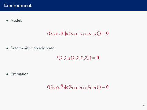
Environment

• Model:

f (xt , yt ,Et [g(xt+1, yt+1, xt , yt)]) = 0

• Deterministic steady state:

f (x , y , g(x , y , x , y)]) = 0

• Estimation:

f (xt , yt , Et [g(xt+1, yt+1, xt , yt)]) = 0

4

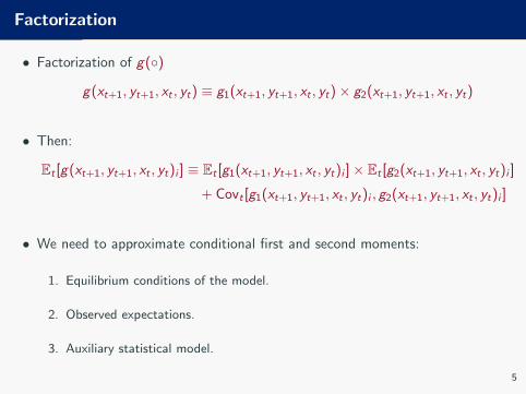
Factorization

• Factorization of g(◦)

g(xt+1, yt+1, xt , yt) ≡ g1(xt+1, yt+1, xt , yt)× g2(xt+1, yt+1, xt , yt)

• Then:

Et [g(xt+1, yt+1, xt , yt)i ] ≡ Et [g1(xt+1, yt+1, xt , yt)i ]× Et [g2(xt+1, yt+1, xt , yt)i ]

+ Covt [g1(xt+1, yt+1, xt , yt)i , g2(xt+1, yt+1, xt , yt)i ]

• We need to approximate conditional first and second moments:

1. Equilibrium conditions of the model.

2. Observed expectations.

3. Auxiliary statistical model.

5

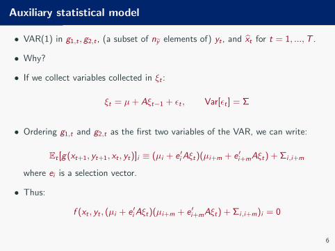
Auxiliary statistical model

• VAR(1) in g1,t , g2,t , (a subset of ny elements of) yt , and xt for t = 1, ...,T .

• Why?

• If we collect variables collected in ξt :

ξt = µ+ Aξt−1 + εt , Var[εt ] = Σ

• Ordering g1,t and g2,t as the first two variables of the VAR, we can write:

Et [g(xt+1, yt+1, xt , yt)]i ≡ (µi + e′iAξt)(µi+m + e′i+mAξt) + Σi,i+m

where ei is a selection vector.

• Thus:

f (xt , yt , (µi + e′iAξt)(µi+m + e′i+mAξt) + Σi,i+m)i = 0

6

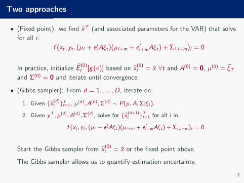
Two approaches

• (Fixed point): we find xT (and associated parameters for the VAR) that solve

for all i :

f (xt , yt , (µi + e′iAξt)(µi+m + e′i+mAξt) + Σi,i+m)i = 0

In practice, initialize E(0)t [g(◦)] based on x

(0)t = x ∀t and A(0) = 0, µ(0) = ξT

and Σ(0) = 0 and iterate until convergence.

• (Gibbs sampler): From d = 1, . . . ,D, iterate on:

1. Given {x (d)t }Tt=1, µ(d),A(d),Σ(d) ∼ P(µ,A,Σ|ξt).

2. Given yT , µ(d),A(d),Σ(d), solve for {x (d+1)t }Tt=1 for all i in:

f (xt , yt , (µi + e′iAξt)(µi+m + e′i+mAξt) + Σi,i+m)i = 0

Start the Gibbs sampler from x(0)t = x or the fixed point above.

The Gibbs sampler allows us to quantify estimation uncertainty.

7

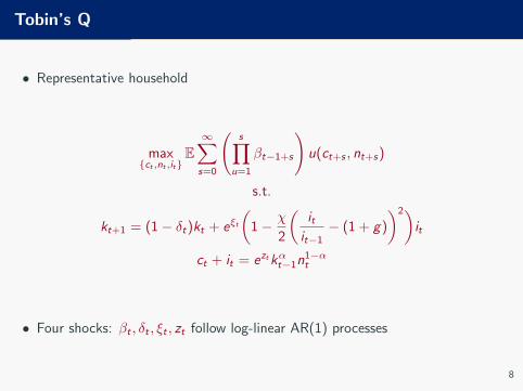
Tobin’s Q

• Representative household

max{ct ,nt ,it}

E∞∑s=0

(s∏

u=1

βt−1+s

)u(ct+s , nt+s)

s.t.

kt+1 = (1− δt)kt + eξt(

1− χ

2

(itit−1− (1 + g)

)2)it

ct + it = eztkαt−1n1−αt

• Four shocks: βt , δt , ξt , zt follow log-linear AR(1) processes

8

Solution (I)

c−ηt (1− κ(1− η)n1+1/φt )1−η = λt

c1−ηt (1− κ(1− η)n

1+1/φt )−η(1 + 1/φ)κ(1− η)n

1/φt = λt(1− α)ezt

(kt−1

nt

)α

λt = µteξt

(1− χ

2

(itit−1− (1 + g)

)2

− χ(

itit−1− (1 + g)

)itit−1

)

+βtEt

[µt+1χ

(it+1

it− (1 + g)

)(it+1

it

)2]

µt = βtEt

[(1− δt+1)µt+1 + λt+1αe

zt+1

(nt+1

kt

)1−α]

9

Solution (II)

c−ηt (1− κ(1− η)n1+1/φt )1−η = λt

c1−ηt (1− κ(1− η)n

1+1/φt )−η(1 + 1/φ)κ(1− η)n

1/φt = λt(1− α)ezt

(kt−1

nt

)α

1 = qteξt

(1− χ

2

(itit−1− (1 + g)

)2

− χ(

itit−1− (1 + g)

)itit−1

)

+Et

[βtλt+1

λtqt+1χ

(it+1

it− (1 + g)

)(it+1

it

)2]

qt = Et

[βtλt+1

λt

((1− δt+1)qt+1 + rkt+1

)]where rkt ≡ αezt+1

(nt+1

kt

)1−α

10

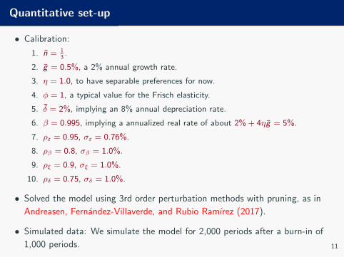
Quantitative set-up

• Calibration:

1. n = 13.

2. g = 0.5%, a 2% annual growth rate.

3. η = 1.0, to have separable preferences for now.

4. φ = 1, a typical value for the Frisch elasticity.

5. δ = 2%, implying an 8% annual depreciation rate.

6. β = 0.995, implying a annualized real rate of about 2% + 4ηg = 5%.

7. ρz = 0.95, σz = 0.76%.

8. ρβ = 0.8, σβ = 1.0%.

9. ρξ = 0.9, σξ = 1.0%.

10. ρδ = 0.75, σδ = 1.0%.

• Solved the model using 3rd order perturbation methods with pruning, as in

Andreasen, Fernandez-Villaverde, and Rubio Ramırez (2017).

• Simulated data: We simulate the model for 2,000 periods after a burn-in of

1,000 periods. 11

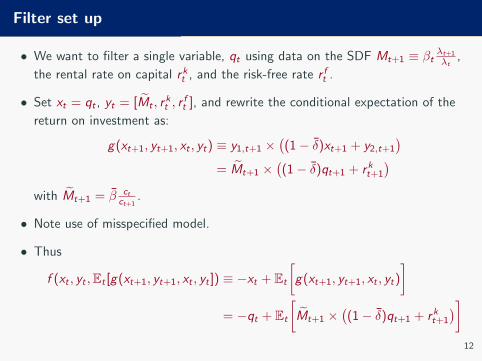
Filter set up

• We want to filter a single variable, qt using data on the SDF Mt+1 ≡ βt λt+1

λt,

the rental rate on capital rkt , and the risk-free rate r ft .

• Set xt = qt , yt = [Mt , rkt , r

ft ], and rewrite the conditional expectation of the

return on investment as:

g(xt+1, yt+1, xt , yt) ≡ y1,t+1 ×((1− δ)xt+1 + y2,t+1

)= Mt+1 ×

((1− δ)qt+1 + rkt+1

)with Mt+1 = β ct

ct+1.

• Note use of misspecified model.

• Thus

f (xt , yt ,Et [g(xt+1, yt+1, xt , yt ]) ≡ −xt + Et

[g(xt+1, yt+1, xt , yt)

]= −qt + Et

[Mt+1 ×

((1− δ)qt+1 + rkt+1

)]12

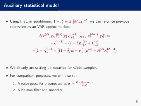
Auxiliary statistical model

• Using that, in equilibrium, 1 + r ft ≡ Et [Mt+1]−1, we can re-write previous

expression as an VAR approximation:

f (x(d)t , yt , E(d)

t [g(x(d−1)t+1 , yt+1, x

(d−1)t , yt ]) ≈

−x (d−1)t + (1− δ)Σ

(d)1,4 + Σ

(d)1,2

+(1 + r ft )−1 ×((1− δ)e4 + e1

)(µ(d) + A(d)X

(d−1)t )

• We already are setting up notation for Gibbs sampler.

• For comparison purposes, we will also run:

1. A naive guess for q computed as qt =(1−δ)+mpkt+1

1+r ft.

2. A Kalman filter and smoother.

13

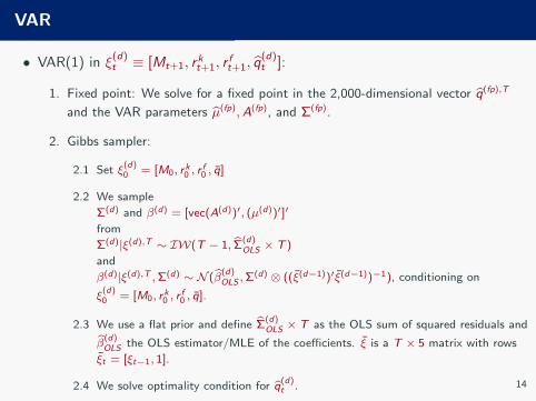
VAR

• VAR(1) in ξ(d)t ≡ [Mt+1, r

kt+1, r

ft+1, q

(d)t ]:

1. Fixed point: We solve for a fixed point in the 2,000-dimensional vector q(fp),T

and the VAR parameters µ(fp),A(fp), and Σ(fp).

2. Gibbs sampler:

2.1 Set ξ(d)0 = [M0, rk0 , r

f0 , q]

2.2 We sample

Σ(d) and β(d) = [vec(A(d))′, (µ(d))′]′

from

Σ(d)|ξ(d),T ∼ IW(T − 1, Σ(d)OLS × T )

and

β(d)|ξ(d),T ,Σ(d) ∼ N (β(d)OLS ,Σ

(d) ⊗ ((ξ(d−1))′ξ(d−1))−1), conditioning on

ξ(d)0 = [M0, rk0 , r

f0 , q].

2.3 We use a flat prior and define Σ(d)OLS × T as the OLS sum of squared residuals and

β(d)OLS the OLS estimator/MLE of the coefficients. ξ is a T × 5 matrix with rows

ξt = [ξt−1, 1].

2.4 We solve optimality condition for q(d)t . 14

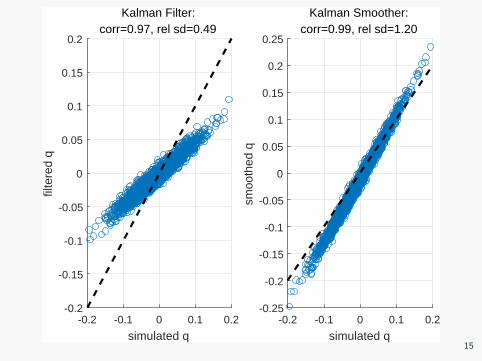
-0.2 -0.1 0 0.1 0.2

simulated q

-0.25

-0.2

-0.15

-0.1

-0.05

0

0.05

0.1

0.15

0.2

0.25

smoo

thed

q

Kalman Smoother:corr=0.99, rel sd=1.20

-0.2 -0.1 0 0.1 0.2

simulated q

-0.2

-0.15

-0.1

-0.05

0

0.05

0.1

0.15

0.2fil

tere

d q

Kalman Filter:corr=0.97, rel sd=0.49

15

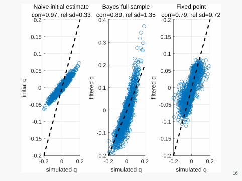
-0.2 0 0.2

simulated q

-0.2

-0.15

-0.1

-0.05

0

0.05

0.1

0.15

0.2in

itial

q

Naive initial estimatecorr=0.97, rel sd=0.33

-0.2 0 0.2

simulated q

-0.2

-0.1

0

0.1

0.2

0.3

0.4

filte

red

q

Bayes full samplecorr=0.89, rel sd=1.35

-0.2 0 0.2

simulated q

-0.2

-0.15

-0.1

-0.05

0

0.05

0.1

0.15

0.2

filte

red

q

Fixed pointcorr=0.79, rel sd=0.72

16

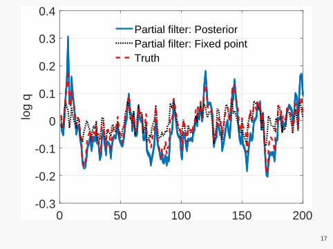
0 50 100 150 200-0.3

-0.2

-0.1

0

0.1

0.2

0.3

0.4lo

g q

Partial filter: PosteriorPartial filter: Fixed pointTruth

17

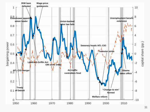
Political distribution risk and aggregate fluctuations

Budd (2012), ‘Labor Relations – Striking a Balance,’ 4th ed.

A popular framework for thinking about labor law is to consider a pendulum that

can range from strong bargaining power for labor . . . to strong bargaining

power for companies . . . .

We stress the role that changes in

1. statutory labor law (including executive orders),

2. case law (courts and NLRB), and

3. political climate

have on business cycles, income shares, and asset prices.

18

Model

• RBC model with search and matching frictions.

(Andolfatto, 1996; Merz, 1995; Shimer, 2010)

• Household with a continuum of members. Members are either employed or

unemployed.

• Household insures members against idiosyncratic employment risk.

• Competitive firms that choose recruiting intensity.

• Government.

• Complete markets.

• Bargaining power subject to persistent redistribution shocks.

19

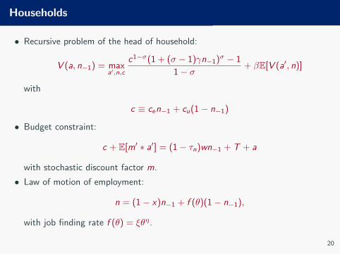
Households

• Recursive problem of the head of household:

V (a, n−1) = maxa′,n,c

c1−σ(1 + (σ − 1)γn−1)σ − 1

1− σ+ βE[V (a′, n)]

with

c ≡ cen−1 + cu(1− n−1)

• Budget constraint:

c + E[m′ ∗ a′] = (1− τn)wn−1 + T + a

with stochastic discount factor m.

• Law of motion of employment:

n = (1− x)n−1 + f (θ)(1− n−1),

with job finding rate f (θ) = ξθη.

20

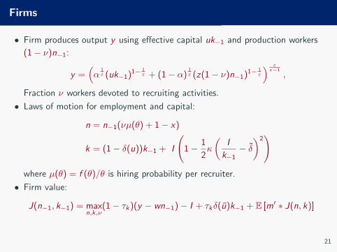
Firms

• Firm produces output y using effective capital uk−1 and production workers

(1− ν)n−1:

y =(α

1ε (uk−1)1− 1

ε + (1− α)1ε (z(1− ν)n−1)1− 1

ε

) εε−1

,

Fraction ν workers devoted to recruiting activities.

• Laws of motion for employment and capital:

n = n−1(νµ(θ) + 1− x)

k = (1− δ(u))k−1 + I

(1− 1

2κ

(I

k−1− δ)2)

where µ(θ) = f (θ)/θ is hiring probability per recruiter.

• Firm value:

J(n−1, k−1) = maxn,k,ν

(1− τk)(y − wn−1)− I + τkδ(u)k−1 + E [m′ ∗ J(n, k)]

21

Wage determination

• Generalized Nash bargaining between firms and households.

• Workers have bargaining power φ.

• Exogenous shifts in φ capture political shocks to bargaining process (Binmore et

al., 1986).

• Other bargaining protocols? (Hall and Milgrom, 2008).

• Equilibrium wage solves

w = arg maxw

Vn(w)φJn(w)1−φ,

where Vn and Jn are marginal values of employment for households and firms

given an arbitrary wage w .

• Equilibrium wage along the balanced growth path:

w = φ× (1 + θ)mpl + (1− φ)× σ

1− τn

(γc

1 + (σ − 1)γn

).

22

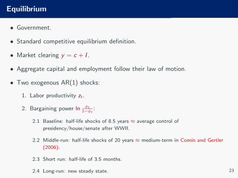
Equilibrium

• Government.

• Standard competitive equilibrium definition.

• Market clearing y = c + I .

• Aggregate capital and employment follow their law of motion.

• Two exogenous AR(1) shocks:

1. Labor productivity zt .

2. Bargaining power ln φt1−φt

:

2.1 Baseline: half-life shocks of 8.5 years ≈ average control of

presidency/house/senate after WWII.

2.2 Middle-run: half-life shocks of 20 years ≈ medium-term in Comın and Gertler

(2006).

2.3 Short run: half-life of 3.5 months.

2.4 Long-run: new steady state. 23

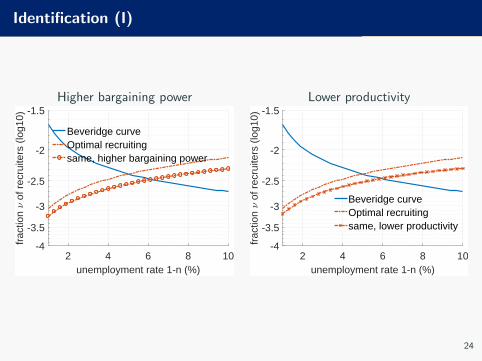
Identification (I)

Higher bargaining power Lower productivity

2 4 6 8 10unemployment rate 1-n (%)

-4

-3.5

-3

-2.5

-2

-1.5

frac

tion

of r

ecru

iters

(lo

g10)

Beveridge curveOptimal recruitingsame, higher bargaining power

2 4 6 8 10unemployment rate 1-n (%)

-4

-3.5

-3

-2.5

-2

-1.5

frac

tion

of r

ecru

iters

(lo

g10)

Beveridge curveOptimal recruitingsame, lower productivity

24

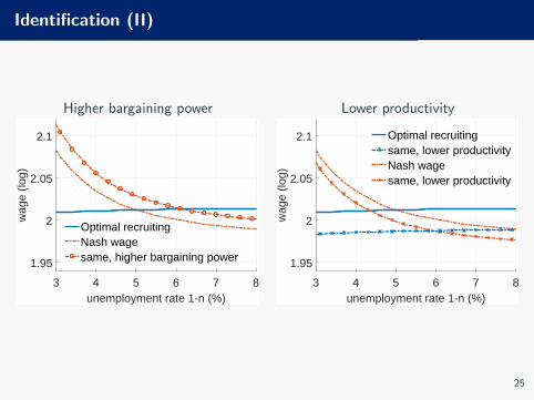
Identification (II)

Higher bargaining power Lower productivity

3 4 5 6 7 8unemployment rate 1-n (%)

1.95

2

2.05

2.1

wag

e (lo

g)

Optimal recruitingNash wagesame, higher bargaining power

3 4 5 6 7 8unemployment rate 1-n (%)

1.95

2

2.05

2.1

wag

e (lo

g)

Optimal recruitingsame, lower productivityNash wagesame, lower productivity

25

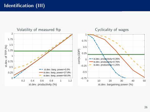
Identification (III)

Volatility of measured ftp Cyclicality of wages

0.2 0.4 0.6 0.8 1 1.2

st.dev. productivity (%)

0

0.25

0.5

0.75

1

1.25

1.5

1.75

2

st.d

ev. o

f TF

P (

%)

st.dev. barg. power=0.0%st.dev. barg. power=27.8%st.dev. barg. power=50.0%

0 10 20 30 40 50

st.dev. bargaining power (%)

-0.75

-0.5

-0.25

0

0.25

0.5

0.75

1

corr

(w,G

DP

)

st.dev. productivity=0.26%st.dev. productivity=0.76%st.dev. productivity=1.25%

26

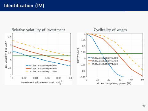
Identification (IV)

Relative volatility of investment Cyclicality of wages

0 0.02 0.04 0.06 0.08 0.1

investment adjustment cost /02

2

2.5

3

3.5

4

4.5

rel.

vola

tility

: I to

GD

P

st.dev. productivity=0.26%st.dev. productivity=0.76%st.dev. productivity=1.25%

0 10 20 30 40 50

st.dev. bargaining power (%)

-0.75

-0.5

-0.25

0

0.25

0.5

0.75

1

corr

(w,G

DP

)

st.dev. productivity=0.26%st.dev. productivity=0.76%st.dev. productivity=1.25%

27

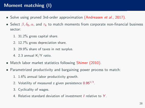
Moment matching (I)

• Solve using pruned 3rd-order approximation (Andreasen et al., 2017).

• Select β, δ0, α, and τk to match moments from corporate non-financial business

sector:

1. 31.2% gross capital share.

2. 12.7% gross depreciation share.

3. 29.9% share of taxes in net surplus.

4. 2.3 annual K/Y ratio.

• Match labor market statistics following Shimer (2010).

• Parametrized productivity and bargaining power process to match:

1. 1.6% annual labor productivity growth.

2. Volatility of measured z given persistence 0.951/3.

3. Cyclicality of wages.

4. Relative standard deviation of investment I relative to Y .

28

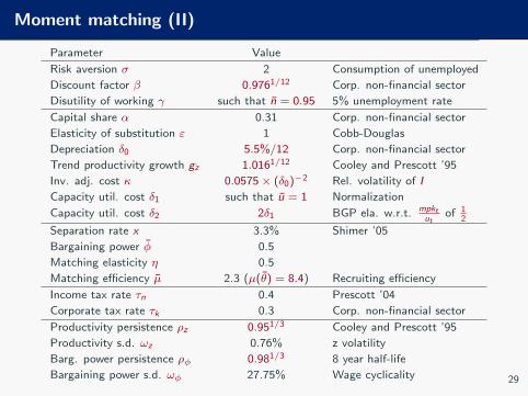
Moment matching (II)

Parameter Value

Risk aversion σ 2 Consumption of unemployed

Discount factor β 0.9761/12 Corp. non-financial sector

Disutility of working γ such that n = 0.95 5% unemployment rate

Capital share α 0.31 Corp. non-financial sector

Elasticity of substitution ε 1 Cobb-Douglas

Depreciation δ0 5.5%/12 Corp. non-financial sector

Trend productivity growth gz 1.0161/12 Cooley and Prescott ’95

Inv. adj. cost κ 0.0575× (δ0)−2 Rel. volatility of I

Capacity util. cost δ1 such that u = 1 Normalization

Capacity util. cost δ2 2δ1 BGP ela. w.r.t. mpktut

of 12

Separation rate x 3.3% Shimer ’05

Bargaining power φ 0.5

Matching elasticity η 0.5

Matching efficiency µ 2.3 (µ(θ) = 8.4) Recruiting efficiency

Income tax rate τn 0.4 Prescott ’04

Corporate tax rate τk 0.3 Corp. non-financial sector

Productivity persistence ρz 0.951/3 Cooley and Prescott ’95

Productivity s.d. ωz 0.76% z volatility

Barg. power persistence ρφ 0.981/3 8 year half-life

Bargaining power s.d. ωφ 27.75% Wage cyclicality 29

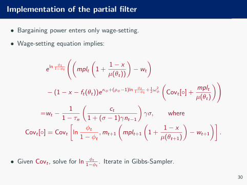
Implementation of the partial filter

• Bargaining power enters only wage-setting.

• Wage-setting equation implies:

e ln φt1−φt

((mplt

(1 +

1− x

µ(θt))

)− wt

)

− (1− x − ft(θt))eκφ+(ρφ−1)ln φt1−φt

+ 12ω

2φ

(Covt [◦] +

mpltµ(θt)

))

=wt −1

1− τn

(ct

1 + (σ − 1)γnt−1

)γσ, where

Covt [◦] = Covt

[ln

φt1− φt

,mt+1

(mplt+1

(1 +

1− x

µ(θt+1)

)− wt+1

)].

• Given Covt , solve for ln φt

1−φt. Iterate in Gibbs-Sampler.

30

1950 1960 1970 1980 1990 2000 20100

0.1

0.2

0.3

0.4

0.5

0.6

0.7

0.8

0.9

1ba

rgai

ning

pow

er

-10

-8

-6

-4

-2

0

2

4

6

8

10

capi

tal s

hare

(pp

.)

Treatyof Detroit

Eisenhower appointsunion leader

AFL-CIO merger

RtW lawsdefeated

Landrum-Griffin Act

Wage-priceguideposts

GM strike ends

Union-backedlabor law fails

Air-trafficcontrollers fired

Sweeney heads AFL-CIO

Welfare reform

Teamster strike

‘‘Change to win''formed

Unemployment benefitextension

Obamatakes office

31

Concluding remarks

• We have other implementations.

• For example: sticky leverage of Gomes, Jermann, and Schmid (2016).

• However, many things to do:

1. Embedding the model in an RBC model could aid in the calibration.

2. Can we use machine-learning tools to improve the covariance/expectations

computation?

3. Heterogeneous agent model.

4. Small sample results.

5. Role for state smoothing due to estimation uncertainty/approximation error.

32