Filtros Digitales 2

Juan-Pablo CaceresCCRMA

Stanford University

Agosto, 2007

Contents

A simple lowpass filter

Determining the frequency reponse

Transfer Function

Linearity and Time Invariance properties

Canonical Forms

Impulse Response

Filtering as Convolution

Z Transform

Basic Filter Sections

A simple lowpass filter

Let’s get back to our Echoplex example.Let’s consider that the Delay is just 1 Sample

x[n] z−1

x[n − 1]y[n]

This filter can be described by the following Difference Equation:

y[n] = x[n] + x[n − 1], n = 0, 1, 2, 3, . . .

Remember that if T is the sampling period, then:

y(nT ) = x(nT ) + x((n − 1)T ), n = 0, 1, 2, 3, . . .

Usage example

Let’s use this x[n] = {1, 2, 3, 4, 5, 6, 7, 8} it our equation

y[n] = x[n] + x[n − 1]

Time Actual time Delayed input Outputn x[n] x[n − 1] y[n]

0 1 - -1 2 1 32 3 2 53 4 3 74 5 4 95 6 5 116 7 6 137 8 7 15

Note that y[0] is not defined as x[−1] is not defined either.

Determining the frequency response

We can determine the frequency response in three ways:

1. Experimental : we send different frequencies to the filter andwe measure the magnitude response

2. Analitic: we insert various sine waves in the Difference

Equation

3. Theoretical : we derive a formula for the response directlyfrom the Difference Equation

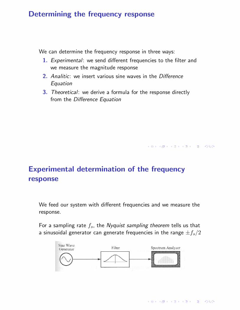
Experimental determination of the frequency

response

We feed our system with different frequencies and we measure theresponse.

For a sampling rate fs, the Nyquist sampling theorem tells us thata sinusoidal generator can generate frequencies in the range ±fs/2

Experimental determination of the frequency

response

We feed out system with sines of 8 different frequencies and weget an approximation to the frequency response:

Analitical determination of the frequency response

Instead of feeding out system signals we can analyze itmathematically, with the following advantages:

◮ We get exact results

◮ We avoid experimental errors

Out test signal will be a cosine

In the difference equation y[n] = x[n] + x[n − 1] we use:

x[n] = A cos[2πfnT + φ]

with A: amplitude, f : frequency, T : sampling period

y[n] = A cos[2πfnT + φ] + A cos[2πf(n − 1)T + φ]

Evaluation for some particular cases

y[n] = A cos[2πfnT + φ] + A cos[2πf(n − 1)T + φ]

Let’s evaluate what happens for the two limit frequencies for oursignal

1. f = 0: DC (Direct Current)

2. f = fs/2: Nyquist frequency

for f = 0:

y[n] = A cos φ + A cos φ

= 2A cos φ

for A = 1 and φ = 0

y[n] = 2

for f = fs/2:1

y[n] = A(−1)n cos φ + A(−1)n−1 cos φ

= A(−1)n cos φ − A(−1)n cos φ

= 0

y[n] = 0

1home work: prove that

A cos(πn + φ) = A(−1)n cos φ

Theoretical determination of the frequency response

Problems with the two previous methods:

We test one frequency at a time

So, let’s use as input a complex sine:

x[n] = Aej(2πfnt+φ)

With ω = 2πf , A = 0 y φ = 0 ⇒ x[n] = ejωnT ,

y[n] = x[n] + x[n − 1]

= ejωnT + ejω(n−1)T

= ejωnT + ejωnT e−jωT

= (1 + e−jωT )ejωnT

= (1 + e−jωT )x[n]

Transfer Function

y[n] = (1 + e−jωT )x[n]

Transfer Function of the lowpass filter

H(ejωT ) = (1 + e−jωT )

We can rewrite our equation as:

y[n] = H(ejωT )x[n]

for f = 0:

H(ejωT ) = H(e0)

= (1 + e−0)

= (1 + 1) = 2

for f = fs/2:

H(ejωT ) = H(ejπ)

= (1 + e−jπ)

= (1 − 1) = 0

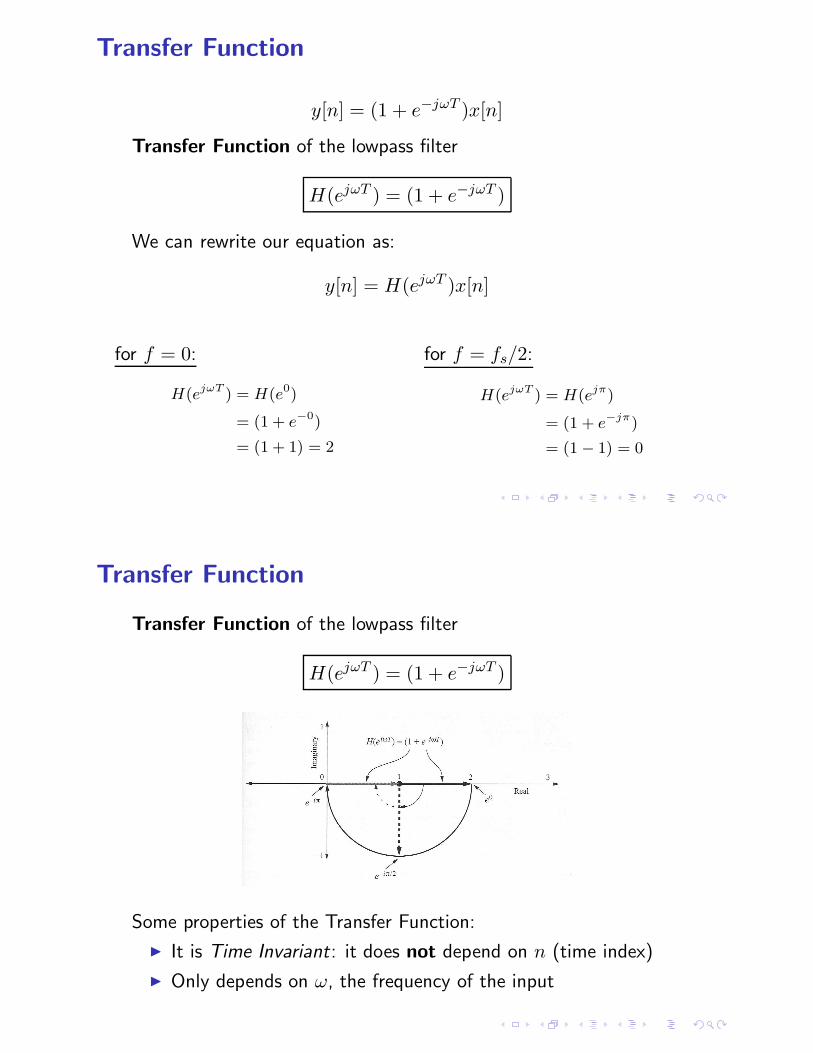
Transfer Function

Transfer Function of the lowpass filter

H(ejωT ) = (1 + e−jωT )

Some properties of the Transfer Function:

◮ It is Time Invariant: it does not depend on n (time index)

◮ Only depends on ω, the frequency of the input

Amplitud Response, Phase Response

There are two things a filter does to a signal:

1. Changes the Amplitude as a function of frequency

2. Changes the Phase as a function of frequency

So, we can define:

1. Amplited Response: the frequency dependent attribute ofthe Gain Transfer Function

2. Respuesta de Fase: the frequency dependent attribute ofthe Delay de la Transfer Function

G(ω) , |H(ejωT )| Amplitude Response

Θ(ω) , ∠H(ejωT ) Phase Response

H(ejωT ) = G(ω)︸ ︷︷ ︸

Amplitud

ejΘ(ω)︸ ︷︷ ︸

Fase

Amplitude and Phase response of the lowpass filterFor our lowpass filter:

H(ejωT ) = (1 + e−jωT )

= (ejωT/2 + e−jωT/2)e−jωT/2

= 2cosωT

2(e−jωT/2)

It is easy to get:

G(ω) = |2 cosωT

2(e−jωT/2)|

= 2| cosωT

2|

= 2cosωT

2= 2 cos(πfT ), −fs/2 ≤ f ≤ fs/2

and

Θ(ω) = −ωT

2= −πfT = −π

f

fs, −fs/2 ≤ f ≤ fs/2

Amplitude and Phase response fo the lowpass filter

G(ω) = 2 cosωT

2− π ≤ ω ≤ π

Θ(ω) = −ωT

2, −π ≤ ω ≤ π

How to we interpret this linear phase?

Linearity and Time Invariance properties

A filter is Linear if:

1. Its input is proportional to its output

2. The ouput is the same for:◮ Input signals are first added and then filtered◮ Input signals are first filtered and then added

L{αx1 + βx2} = αL{x1} + βL{x2}

Dynamic compression is anexample of Non-Linear Filter

Linearity and Time Invariance properties

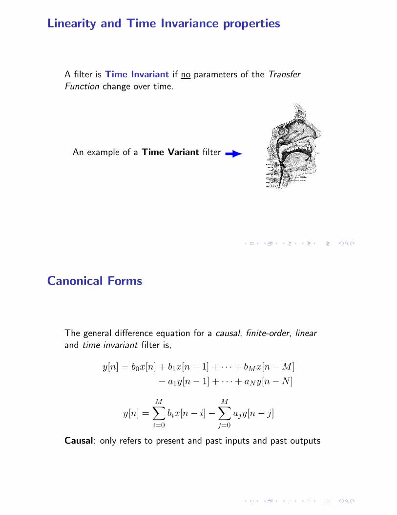
A filter is Time Invariant if no parameters of the Transfer

Function change over time.

An example of a Time Variant filter

Canonical Forms

The general difference equation for a causal, finite-order, linear

and time invariant filter is,

y[n] = b0x[n] + b1x[n − 1] + · · · + bMx[n − M ]

− a1y[n − 1] + · · · + aNy[n − N ]

y[n] =

M∑

i=0

bix[n − i] −

M∑

j=0

ajy[n − j]

Causal: only refers to present and past inputs and past outputs

Canonical Forms, Flow Diagram

y[n] = b0x[n] + b1x[n − 1] + b2x[n − 2] − a1y[n − 1] + a2y[n − 2]

Impulse Response

To characterize filters in the time domain (as opposed to thefrequency domain):

◮ We could apply signals at different frequenciers

◮ We could apply one signal that contains all frequencies

The Unitary Impulse function contains all frequencies

δ[n] ,

{1 n = 00 n 6= 0

Unitary Impulse Function

We define Impulse Response as:

h[n] , L{δ[·]} 2

So we have two characterizations of filters:

1. H(ejωT ): Frequency Response (frequency domain)

2. h[n]: Impulse Response (time domain)

2δ[·] notation is equivalent to δ[n], for n = 0, 1, 2, 3, . . .

An example of impulse response

y[n] = x[n] + 0.9y[n − 1]

= x[n] + 0.9x[n − 1] + 0.92x[n − 1] + · · ·

The reponse to the impulse will be,

h[n] =

{(0.9)n, n ≥ 0

0, n < 0

Filtering as Convolution

Let’s consider the following sampled sin,

x[n] = {0, 0.707, 1, 0.707, 0,−0.707,−1,−0.707, . . . }

We can write x[n] as,

x[n] = [0·δ[n]]+[0.707·δ[n−1]]+[1·δ[n−2]]+[0.707·δ[n−3]]+. . .

Which gives us:

y[n] =

n∑

k=0

x[k]δ[n − k]

= x[n] ∗ δ[n]

= δ[n] ∗ x[n]

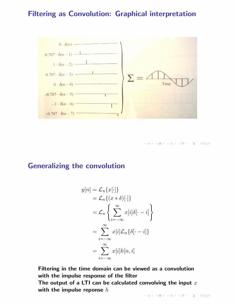
Filtering as Convolution: Graphical interpretation

Generalizing the convolution

y[n] = Ln{x[·]}

= Ln{(x ∗ δ)[·]}

= Ln

{∞∑

i=−∞

x[i]δ[· − i]

}

=

∞∑

i=−∞

x[i]Ln{δ[· − i]}

=

∞∑

i=−∞

x[i]h[n, i]

Filtering in the time domain can be viewed as a convolutionwith the impulse response of the filterThe output of a LTI can be calculated convolving the input xwith the impulse reponse h

Z Transform

Z(z) =

∞∑

n=0

x[n]z−n Z Transform

A shorthand for this notation is

X = Z{x}

Z Transform theorems

Theorem (Shift)

x[n −△] ↔ z−△X(z), △ ≥ 0

Theorem (Convolution)

x ∗ y ↔ X · Y

Z Transform of the Convolution

If we have,y[n] = (h ∗ x)[n]

Take the Z transform on both sides of the equaction,

Y (z) = H(z) · X(z)

We can finally obtain the Transfer Function,

H(z) =Y (z)

X(z)Transfer Function

This comes directly from the Convolution Theorem and appliesprovided that the filter is LTI.

Z Transform of the Difference Equation

For our generic difference equation case,

y[n] = b0x[n] + b1x[n − 1] + · · · + bMx[n − M ]

− a1y[n − 1] + · · · + aNy[n − N ]

Taking the Z Transform on both sides of the equation,

Z{y[·]} = Z{b0x[n] + b1x[n − 1] + · · · + bMx[n − M ]

− a1y[n − 1] + · · · + aNy[n − N ]}

= Z{b0x[n]} + Z{b1x[n − 1]} + · · · + Z{bMx[n − M ]}

− Z{a1y[n − 1]} + · · · + aNZ{y[n − N ]}

= b0X(z) + b1z−1X(z) + · · · + bMz−MX(z)

− a1z−1Y (z) + · · · + aNz−NY (z)

Z Transform of the Difference Equation

We define,A(z) = 1 + a1z

−1 + · · · + aNz−N

B(z) = b0 + b1z−1 + · · · + bMz−M

Rearranging the equations,

H(z) =Y (z)

X(z)=

b0 + b1z−1 + · · · + bMz−M

1 + a1z−1 + · · · + aNz−N=

B(z)

A(z)

Deriving the Frequency Response

To obtain the Frequency Response it is enough to replace z in thetransfer function with,

z = ejωT

That is, if we have a transfer function H(z), the frequencyresponse is,

H(ejωT )

Basic Filter Sections: One Zero

One Zero filters,

y[n] = b0x[n] + b1x[n − 1]

One Zero

One Pole

One Pole filters,

y[n] = b0x[n] − a1y[n − 1]

One Pole

Two PoleTwo Pole filters,

y[n] = b0x[n] − a1y[n − 1] − a2y[n − 2]

Two Pole

Two Zero

Two Zero filters,

y[n] = b0x[n] + b1x[n − 1] + b2x[n − 2]

Two Zero

Allpass Filters

If we take a Biquad transfer function,

H(z) = g1 + β1z

−1 + β2z−2

1 + a1z−1 + a2z−2

An Allpass filter requires that,

|H(ejωT )| = 1

For this to be true the Biquad has to meet this requirement,

B(z) = z−2A(z−1) = a2 + a1z−1 + z−2

Conclusions

The selection of a filter implies a compromise between,

◮ Precision of desired response vs. computational load

◮ “Warm-up” time

◮ Selecting between IIR and FIR,◮ IIR are more efficient but introduce phase distortion.◮ Longer impulse responses are needed to get the same

frequency response with a FIR filter