FIN822 project 3 (Due on December 15. Accept printout submission or email submission donglinli2006@yahoo.com. ) Part I The Fama-French Multifactor Model and Mutual Fund Returns

Dawn Browne, an investment broker, has been approached by client Jack Thomas about the risk of his investments. Dawn has recently read several articles concerning the risk factors that can potentially affect asset returns, and she has decided to examine Jack's mutual fund holdings. Jack is currently invested in the Fidelity Magellan Fund (FMAGX), the Fidelity Low-Priced Stock Fund (FLPSX), and the Baron Small Cap Fund (BSCFX).

Dawn would like to estimate the well-known multifactor model proposed by Eugene Fama and Ken French to determine the risk of each mutual fund. Here is the regression equation for the multifactor model she proposes to use:

1 2( ) ( ) (it Ft i Mt FT t tR R R R SMB HM3 ) tLα β β β− = + − + + ε+

In the regression equation, Rit, is the return of asset i at time t, RFt:, is the risk-free rate at time t, and Rmt is the return on the market index at time t. Thus, the first risk factor in the Fama–French regression is the market factor often used with the CAPM.

The second risk factor, SMB or "small minus big," is calculated by taking the difference in the returns on a portfolio of small-cap (cap=capitalization her) stocks and a portfolio of big-cap stocks. This factor is intended to pick up the so-called small firm effect. Similarly, the third factor, HML or "high minus low," is calculated by taking the difference in the returns between a portfolio of "value" stocks (high book-to-market ratio stocks) and a portfolio of "growth" stocks (low book-to-market ratio stocks). Stocks with low market-to-book ratios are classified as value stocks and vice versa for growth stocks. This factor is included because of the historical tendency for value stocks to earn a higher return.

In models such as the one Dawn is considering, the alpha term is of particular interest. It is the regression intercept; but more important, it is also the excess return the asset earned. In other words, if the alpha is positive, the asset earned a return greater than it should have given its level of risk; if the alpha is negative, the asset earned a return lower than it should have given its level of risk. This measure is called "Jensen's alpha," and it is a very widely used tool for mutual fund evaluation.

1. For a large-company stock mutual fund (for example, FMAGX) , would you expect the coefficients to be positive or negative for each of the factors in a Fama–French multifactor model? Why.

2

Hints: Positive and close to 1; negative; Not sure.

How about small company fund (BSCFX) and Low-Priced Stock Fund (FLPSX)?

2. The Fama–French factors and risk-free rates are available at Ken French's Web site: http://mba.tuck.dartmouth.edu/pages/faculty/ken.french/. (On his website, click Data Library, then click “Fama/French factors detail”. (For your convenience, I already put it on my web http://online.sfsu.edu/~donglin/FF.xls ) Download the monthly factors and save the most recent 60 months (20031031—20081031) for each factor. The historical prices for each of the mutual funds can be found on various Web sites, including finance.yahoo.com. Find the prices of each mutual fund for the same time-period (20031031—20081031) as the Fama–French factors and calculate the returns for each month. Be sure to include dividends. (that is, return should be based on adj. closing price) For each mutual fund, estimate the multifactor regression equation using the Fama–French factors. How well do the regression estimates explain the variation in the return of each mutual fund?

Hints: Goodness of fit, R-squared.

3. What do you observe about the coefficients for each of the factors for the three mutual funds? Comment on any similarities or differences. Hints: This question is related to part 1.

4. If the market is efficient, what value would you expect for alpha? Do your estimates support market efficiency?

Hints: insignificant alpha (=intercept) if market is efficient. 5. Which fund has performed best considering its risk? Why?

Hints: Check alpha.

Part II Accrual Anomaly Download dataset accrual.xls from my web at: http://online.sfsu.edu/~donglin/accrual.xls In the dataset, accrual is defined as:

accrual= (operatingIncomeorLoss- totalCashFlowFromOperatingActivi)/totalassets

1. In the dataset, first sort all observations annually into 5 groups (quintiles)

based the level of accruals. Compute the mean next-year-stock-return within

each quintile. Based on the result would you invest in low accrual stocks or high

accrual stocks?

Hints for Part I:

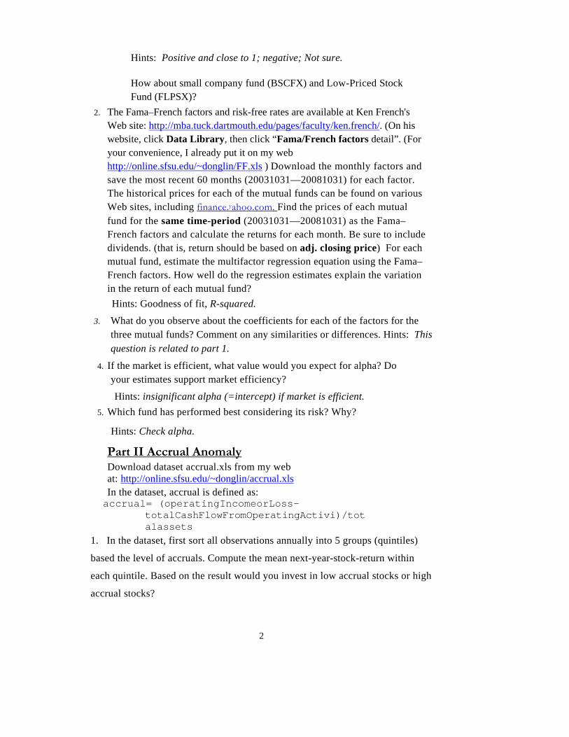
I will take FMAGX for example.

Log on to Yahoo! Finance. Enter the symbol “FMAGX”.

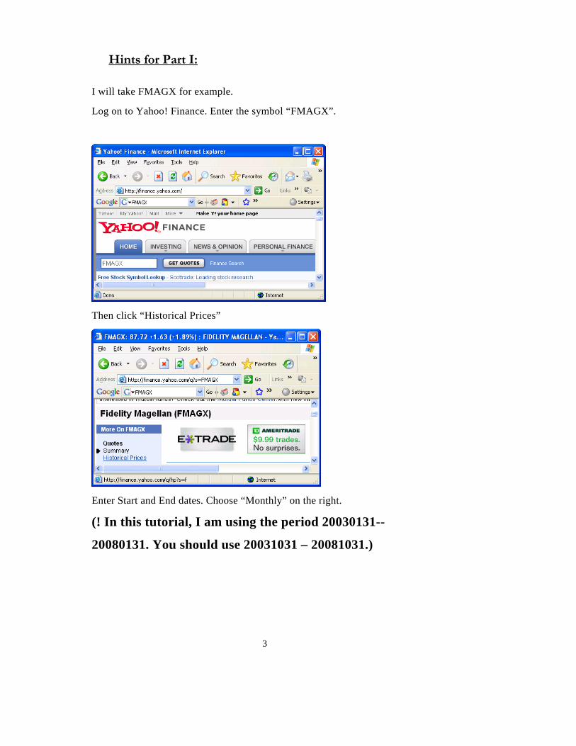
Then click “Historical Prices”

Enter Start and End dates. Choose “Monthly” on the right.

(! In this tutorial, I am using the period 20030131--

20080131. You should use 20031031 – 20081031.)

3

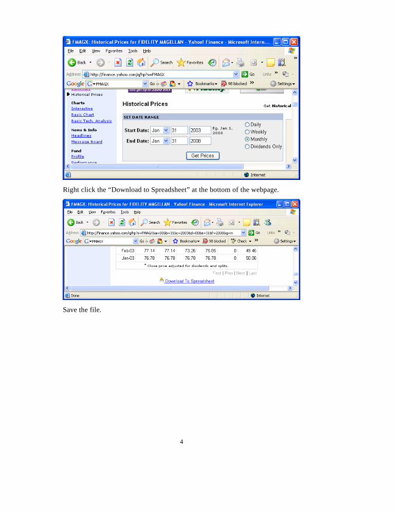
Right click the “Download to Spreadsheet” at the bottom of the webpage.

Save the file.

4

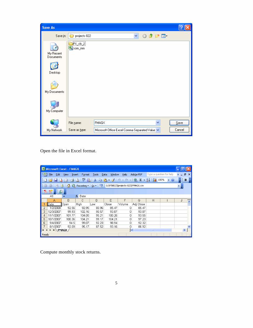
Open the file in Excel format.

Compute monthly stock returns.

5

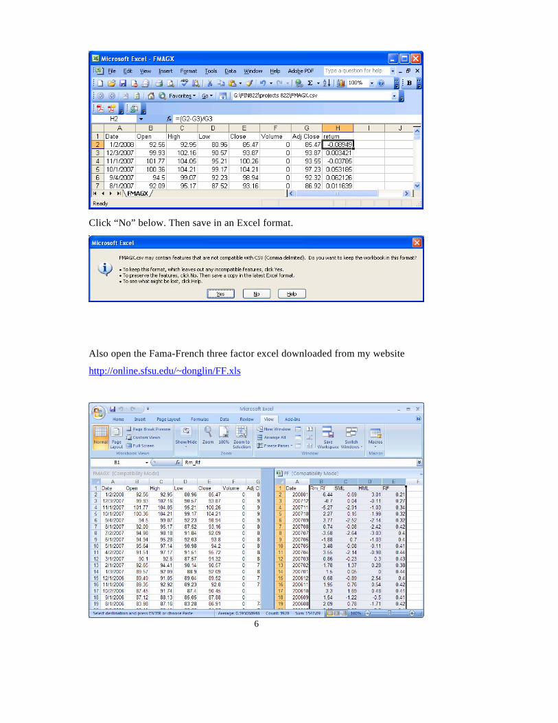
Click “No” below. Then save in an Excel format.

Also open the Fama-French three factor excel downloaded from my website

http://online.sfsu.edu/~donglin/FF.xls

6

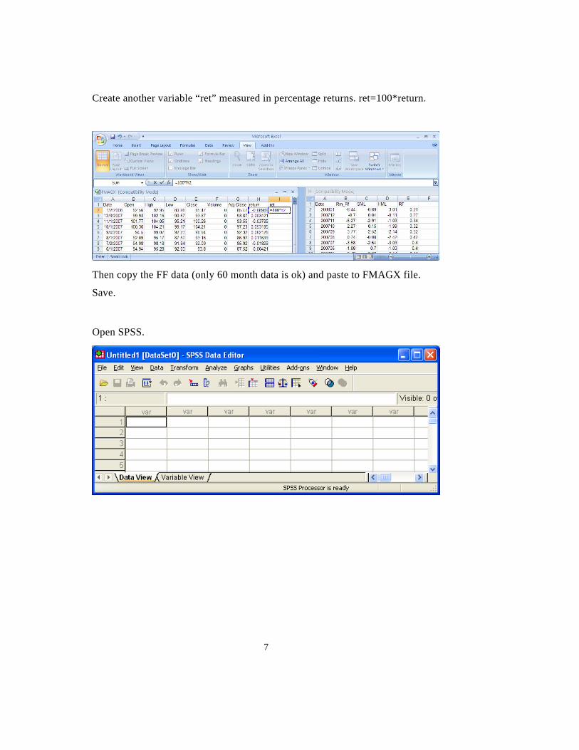
Create another variable “ret” measured in percentage returns. ret=100*return.

Then copy the FF data (only 60 month data is ok) and paste to FMAGX file.

Save.

Open SPSS.

7

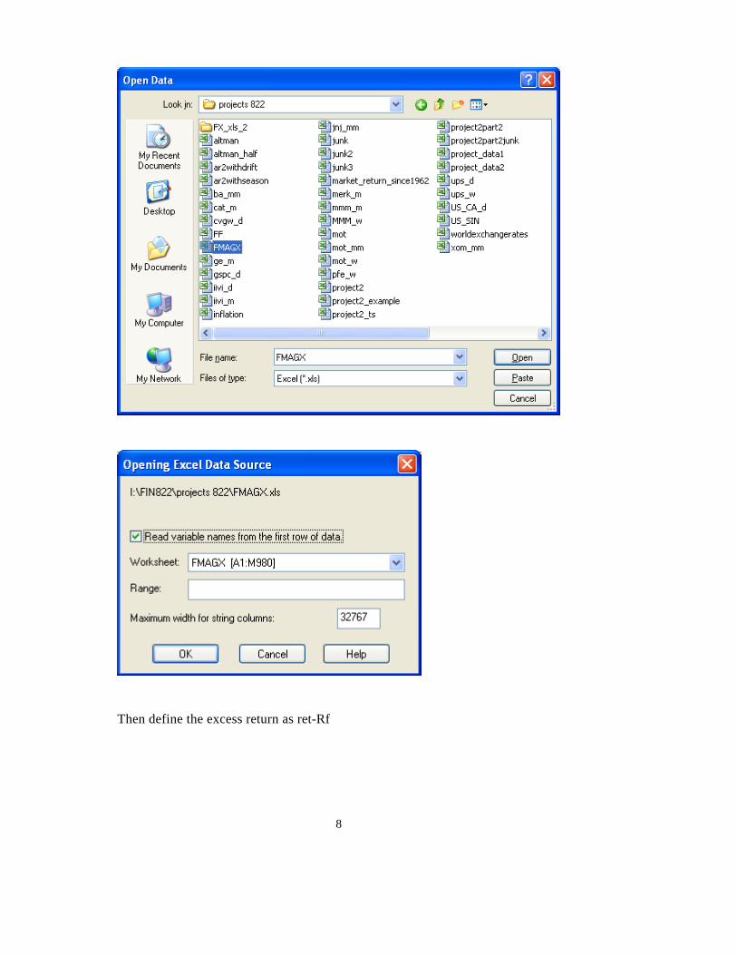
Then define the excess return as ret-Rf

8

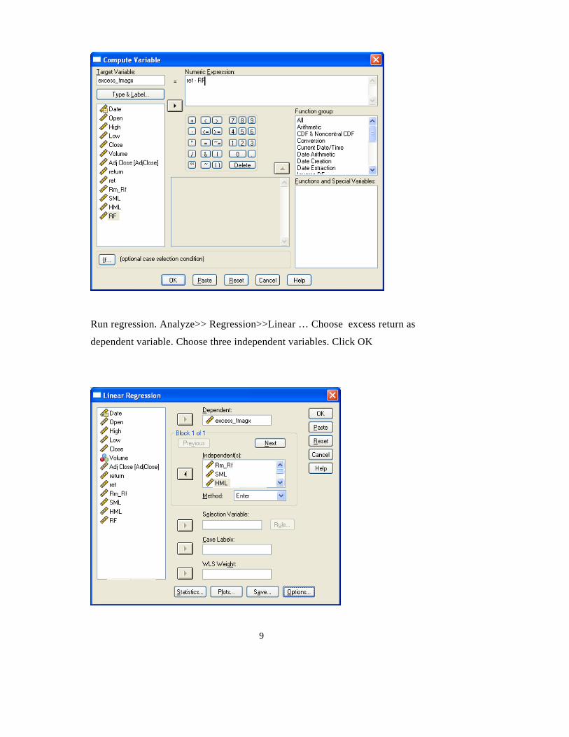
Run regression. Analyze>> Regression>>Linear … Choose excess return as

dependent variable. Choose three independent variables. Click OK

9

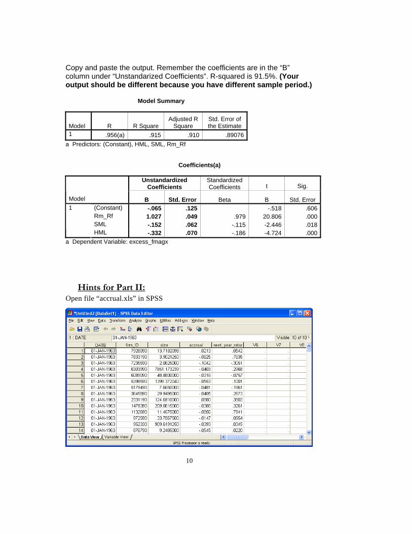
Copy and paste the output. Remember the coefficients are in the “B” column under “Unstandarized Coefficients”. R-squared is 91.5%. (Your output should be different because you have different sample period.) Model Summary

Model R R Square Adjusted R

Square Std. Error of the Estimate

1 .956(a) .915 .910 .89076a Predictors: (Constant), HML, SML, Rm_Rf Coefficients(a)

Unstandardized Coefficients

Standardized Coefficients t Sig.

Model B Std. Error Beta B Std. Error (Constant) -.065 .125 -.518 .606 Rm_Rf 1.027 .049 .979 20.806 .000 SML -.152 .062 -.115 -2.446 .018

1

HML -.332 .070 -.186 -4.724 .000 a Dependent Variable: excess_fmagx

Hints for Part II: Open file “accrual.xls” in SPSS

10

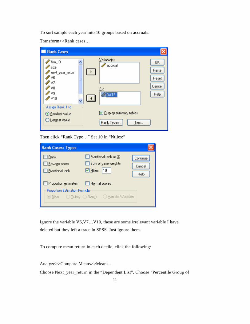
To sort sample each year into 10 groups based on accruals:

Transform>>Rank cases…

Then click “Rank Type…” Set 10 in “Ntiles:”

Ignore the variable V6,V7…V10, these are some irrelevant variable I have

deleted but they left a trace in SPSS. Just ignore them.

To compute mean return in each decile, click the following:

Analyze>>Compare Means>>Means…

Choose Next_year_return in the “Dependent List”. Choose “Percentile Group of 11

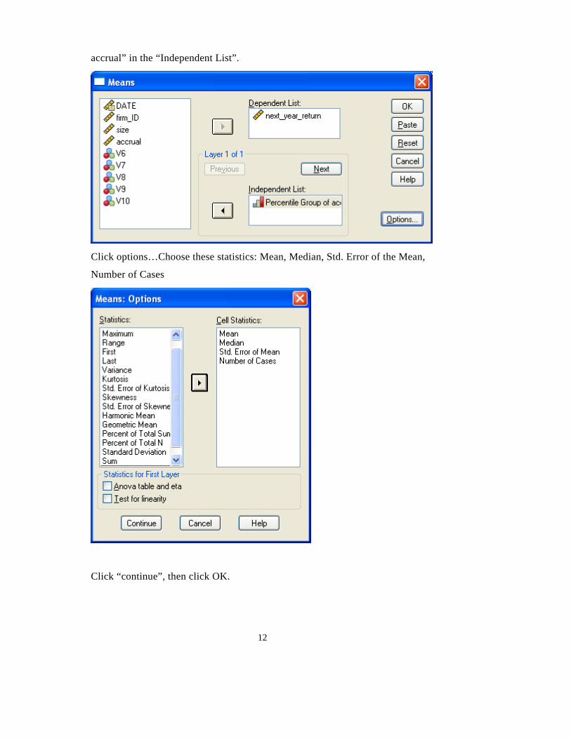
accrual” in the “Independent List”.

Click options…Choose these statistics: Mean, Median, Std. Error of the Mean,

Number of Cases

Click “continue”, then click OK.

12

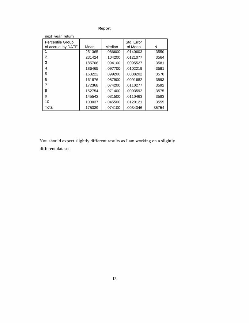
Report

next_year_return

.251365 .086600 .0140603 3550

.231424 .104200 .0121077 3564

.185706 .094100 .0095527 3581

.186465 .097700 .0102219 3591

.163222 .099200 .0088202 3570

.161876 .087900 .0091682 3593

.172368 .074200 .0110277 3592

.152754 .071400 .0093592 3575

.145542 .031500 .0110463 3583

.103037 -.045500 .0120121 3555

.175339 .074100 .0034346 35754

Percentile Groupof accrual by DATE12345678910Total

Mean MedianStd. Errorof Mean N

You should expect slightly different results as I am working on a slightly

different dataset.

13