Final draft Project(485)

Justin Htoo (012854567)

ECON - 485

Instructor: Dr. Jake Meyer

Department of Economics

California State University, Long Beach

Long Beach, California, USA

December 16, 2016

ECON 485- Econometrics 1 December 16, 2016

2

Abstract

Traffic plays a vital role in our daily life. For whatever reason, be it school, work, grocery

shopping for the wives and the kids, doctor appointments, etc., people need to get out of their

house and commute to places. However, commuting also means that people commit to getting into

traffic, mentally and readily preparing themselves to yell, swear, or even get into intense arguments

with their fellow traffic committees. It seems like traffic has a huge effect on people’s happiness.

But, what cannot be seen on the surface is how traffic, which only brings the worst out of people at

that crucial time when they decide to leave the house and get stressed over, would affect the

happiness level of individuals who live in areas with consistently excessive traffic. This paper will

compare the average traffic jams in the major cities in the United States regarding the average level

of happiness in these areas. Apparently, and surprisingly, even though traffic has measurably

negative effect on overall happiness, the effect is not as high as expected and does not account

much for the variation in the level of satisfaction in these areas.


3

Introduction

Living in the major cities means that people have to commute in one way or another.

Otherwise, it is considered a handicap. However, the higher the number of individuals joining

traffic, the more likely traffic jams will happen, and the longer the bottlenecks will be. Taking

many factors into consideration such as time, distance, age, salary, relationship status, poverty,

crime, population, income, and FasTrak, I can break down the effect that traffic has on people’s

level of happiness. For example, the more traffic jams there are, the less happy people are. The

more time one spends on commute equals one’s lost time spending on personal enjoyment,

relaxation, time. The longer the distance means, the longer time one spends on traffic which can

lead to arguments and eventually stresses. The age differences can also affect traffic in a sense that

young people tend to have more occupations (school, work, parties, dating, chill, etc.) and

therefore, they spend more time commuting than older people (65 and over). The higher the salary

one receives, the more likely that person is willing to travel farther distance meaning spending

more time in traffic. If the man is married, he has to be home by a certain time assigned by his

wife. Otherwise, he will not get fed, and will be hungry, and will not be happy during bedtime.

Last but not least, if the person has FasTrak, they tend to have less stress over commuting because

they have to deal less with traffic jams.

Overall, these factors show how traffic and other factors can affect people’s happiness

mostly negatively. The goal of this research project is to demonstrate the correlation between

traffic and people’s level of happiness. With the help of the above-explained factors, plus some

more dummy variables, this project will provide a better understanding of how traffic can affect

people’s happiness.


4

Literature Review Many studies have been conducted on the effect traffic has on people living in cities. One

subject that has been studied well is whether commuters are fully compensated for their lost time in

traffic. Different measures of well-being, including self-reported health and self-reported disability,

have been compared to travel mode and travel time for both commuters and non-commuters.

Compared with non- commuters the report found that on average commuters were “less satisfied

with their lives,” and reported less happiness and higher anxiety. It has been found that with each

additional minute a person commutes, they are expected to experience a decrease in

happiness/satisfaction and an increase in anxiety levels (ONS 2014). This suggests that higher

levels of traffic will lead to unhappier cities.

Semi-random variation in daily traffic has been correlated with self-reported happiness and

used to show that on days where there is more traffic, all citizens are likely to be less happy. Every

week in Beijing, a particular set of license plates based on the ending digit are banned from

traveling within the city center to cut down on traffic demands. Usually, this would remove 1/5th

of the cars from the roads in the city center, however, because the number 4 is superstitious in

China, many fewer cars end in 4 than other numbers. Therefore, on days where the number 4 is

banned it is seen that there are more cars on the road than on the other four days of the week.

Because the day that each tail number banned rotates throughout the month, researchers were able

to assemble a quasi-random dataset where certain days were guaranteed to have more traffic. This

data was confirmed using day by day pollution data taken from within the city center of Beijing.

Using this traffic data and daily self-reported happiness studies, the researchers were able to draw a

close correlation between daily traffic and expected happiness. It was found for each 15% increase

in traffic (i.e. 5mph slower approx.) there was a 1.5% decrease in a person’s happiness. This

statistic remains robust when including weather, pollution levels, and excluding holidays from the


5

data. While this does not show that on the macro level general congestion indices will correlate

with general happiness indices, it does indicate that there is a measurable effect on individual

happiness that comes from sitting in traffic (Anderson et. al. 2016). It remains to be seen whether a

metro area will experience a permanent depression in happiness as a result of high traffic.

Adults in Basel, Switzerland have been studied to measure the relationship between road

traffic, noise exposure, annoyance caused by noise sources, and health factors that could be

affected by traffic. Noise annoyance was evaluated using a four-points Likert scale (categories:

“no,” “slight,” “considerable,” and “heavy”). The research shows that people felt a more obvious

annoyance from road, industry, and neighborhood noise over railway and aircraft noise. A

significant association was found between road traffic noise and objective sleep parameters, but

there was not a significant association between road traffic noise and subjective sleep quality

measures, after controlling for other factors. People are shown to be unaware of the objective

effects of noise on their sleep, though this may have further implications for other health risks such

as cardiovascular disease despite the fact that they do not realize it, and calls into question the

accuracy of “annoyance” as an indicator of individual health effects of noise (Vienneau et. al.

2014).

The NBER paper “Unhappy Cities” contains a dataset that will be useful for my research,

as well as significant research on happiness in major US cities and factors that correlate with them.

A happiness index has been generated that includes all the main metropolitan areas in the United

States. This data was analyzed to look for differences in satisfaction across cities and how these

happiness levels changed over time. There is a significant difference between levels of happiness

in different towns and happiness behave differently with time depending on each city. These

differences persisted even after controlling for income, weather, and inequality. This research also

found that there is a negative correlation between income and happiness, i.e. happier metropolitan


6

areas have lower median incomes. It is speculated that higher wages in unhappy places compensate

for the fact that the locations aren’t right for the resident’s happiness. Higher incomes may be

necessary to support the other ambitions of people who choose to live in unhappy cities even

though they may be happier elsewhere. It is also seen that there is a positive correlation between

population decline and unhappiness. For my research, this would suggest that traffic may

positively correlate with happiness because cities with higher population growth are more likely to

have high stress on their road network (Glaeser et. al. 2016). This is contrary to the intuitive idea

that because traffic decreases individual happiness, traffic will also decrease citywide happiness.

My research will expand on existing research to provide an analysis of how permanent

differences in traffic effect people's self-reported happiness. All of the papers showed that there is a

strong negative correlation between traffic and happiness. However, this does not necessarily mean

that cities as remote units will be more or less happy than other cities based purely on their traffic.

Because cities that are growing have higher rates of happiness, traffic may end up positively

correlating with happiness. A result like this would not disprove existing research of traffic effects,

but it would show that traffic is not a major indicator of whether an area has happy people or not.

My research will attempt to apply the concepts learned from earlier papers and use them across

space to look for permanent differences in happiness as a result of traffic.


7

Data

The dependent variable for this regression model is happiness. This data comes from a

study by Glaeser, Ziv and Gottlieb published by the Journal of Labor Economics (Glaeser et. at.

2016). This paper uses self-reported survey data on subjective well-being from across the United

States, and data from the Center for Disease Control and Prevention (CDC). The survey used from

the CDC is the Behavioral Risk Factor Surveillance System, a self-reporting survey. The authors

modified the original data and scaled the responses 1-4, 4 representing “very satisfied” and 1 as

“very dissatisfied.” The authors manipulate the data in several ways to reduce the bias that may

occur from differences in geography, demographics, and variability in different individuals

measures of happiness. They use the data from the CDC as well as the National Survey of Families

and Households (NSFH). The survey is also self-reported with questions regarding well-being

having a scale of 1-7. The authors use several different methods to manipulate the data to account

for variations that are likely to be attributed to personal tastes rather than circumstances. This

regression model will use the raw data Glaeser, Ziv, and Gottlieb compiled using the different self-

reported survey data.

This report will look at data on 27 major metropolitan cities in the U.S. to see if there is a

significant correlation between levels of self-reported happiness and time spent in traffic. The

independent variable this paper looks at is traffic, specifically, total delay per year in hours by the

city (INTRIX 2016). This study is done annually by INRIX. The most available data from INRIX

is the the “Worst Corridor” analysis which provides a breakdown of different metro cities in the

U.S. This data set contains a breakdown in distance, time, and peak times, and free flow times.

INRIX also provides a calculated “time wasted in traffic annually” estimate. However, it is only

for the top ten “most congested” cities in the U.S.


8

Other independent variables included in the regression include the percentage of

individuals living below the poverty line by the city. This variable is likely correlated to levels of

wellbeing, but not likely correlated to the average amount of time spent in traffic. This data comes

from the United States Census (US Census Bureau). Income per capita (USD) is another

independent variable. Data statistics on income are sourced from the United States Census. Income

is primarily positively associated with happiness but may also have a correlation with time spent in

traffic. Crime rates are likely to have a negative correlation with happiness but are not likely to

have a correlation with the average amount of time spent in traffic. The crime statistics come from

the U.S. Department of Justice. The data is total violent offenses reported per 100,000 people. The

crimes that fall under violent crime include; rape, murder, and robbery. The model will also

include the average percentage of days annually that are either cloudy or partly cloudy. The

amount of sunshine is likely positively correlated with levels of happiness but is not likely to have

any correlation with time spent in traffic. This data comes from the U.S. National Oceanic and

Atmospheric Administration. For each city, the data has been collected over periods of time

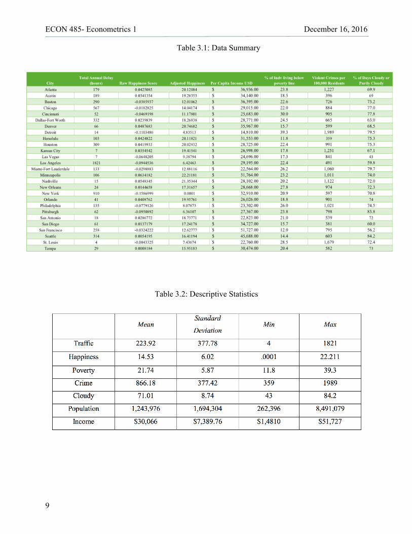
ranging from 30 to 60 years. Table 3.1 below shows the data I used in my analysis. Table 3.2

contains the descriptive statistics.


9

Table 3.1: Data Summary

Table 3.2: Descriptive Statistics


10

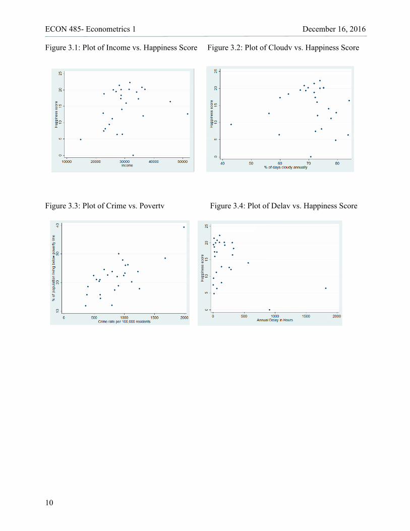
Figure 3.1: Plot of Income vs. Happiness Score Figure 3.2: Plot of Cloudv vs. Happiness Score

Figure 3.3: Plot of Crime vs. Povertv Figure 3.4: Plot of Delav vs. Happiness Score


11

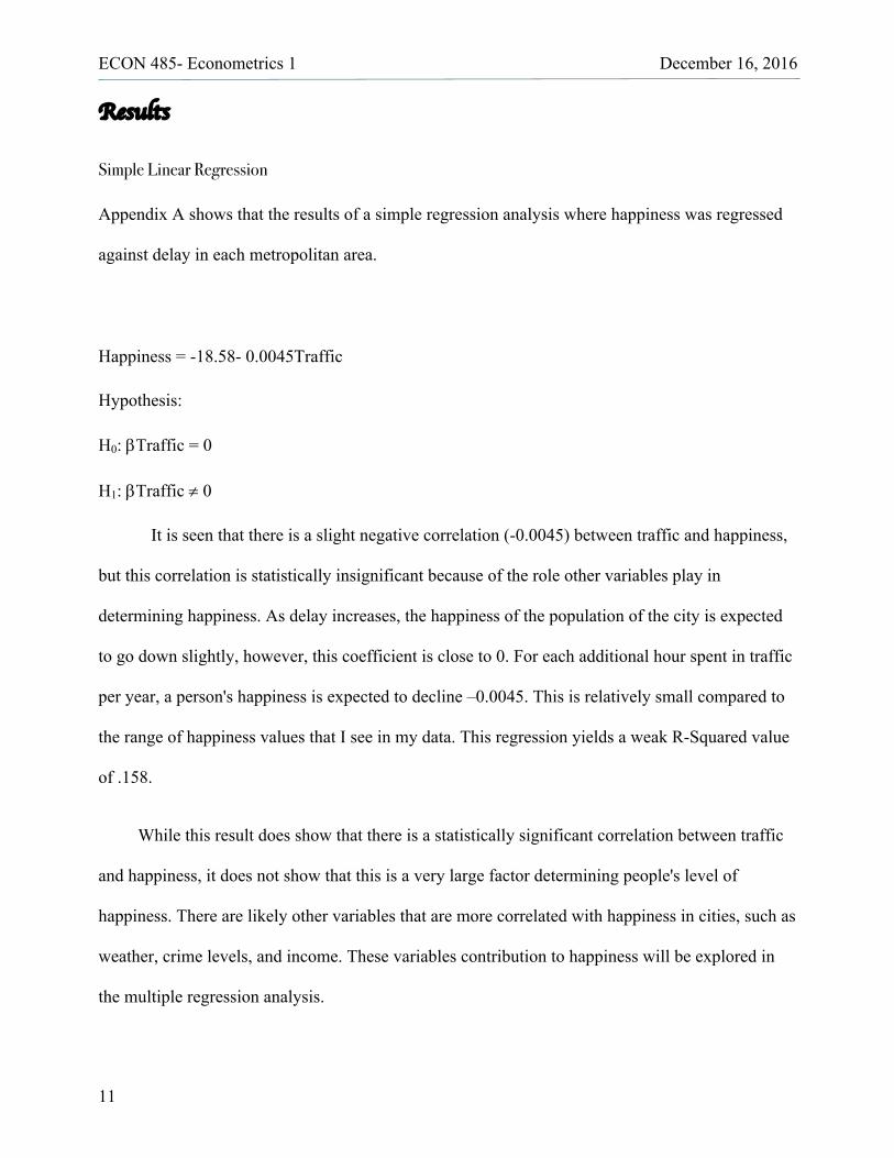
Results

Simple Linear Regression

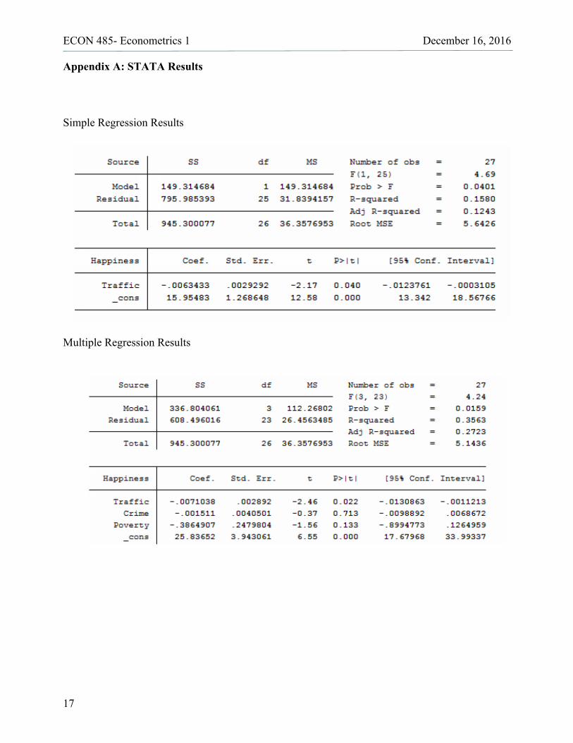
Appendix A shows that the results of a simple regression analysis where happiness was regressed

against delay in each metropolitan area.

Happiness = -18.58- 0.0045Traffic

Hypothesis:

H0: bTraffic = 0

H1: bTraffic ¹ 0

It is seen that there is a slight negative correlation (-0.0045) between traffic and happiness,

but this correlation is statistically insignificant because of the role other variables play in

determining happiness. As delay increases, the happiness of the population of the city is expected

to go down slightly, however, this coefficient is close to 0. For each additional hour spent in traffic

per year, a person's happiness is expected to decline –0.0045. This is relatively small compared to

the range of happiness values that I see in my data. This regression yields a weak R-Squared value

of .158.

While this result does show that there is a statistically significant correlation between traffic

and happiness, it does not show that this is a very large factor determining people's level of

happiness. There are likely other variables that are more correlated with happiness in cities, such as

weather, crime levels, and income. These variables contribution to happiness will be explored in

the multiple regression analysis.


12

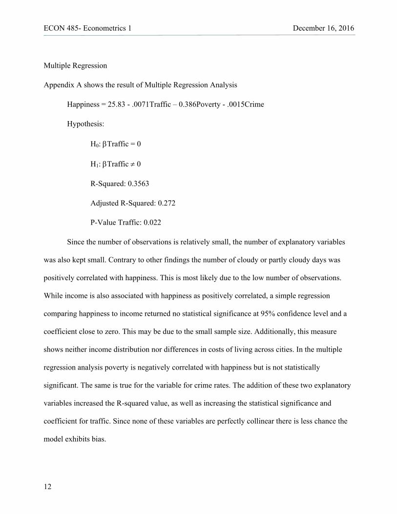
Multiple Regression

Appendix A shows the result of Multiple Regression Analysis

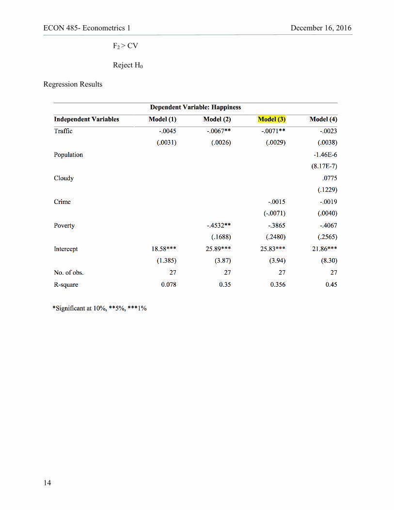
Happiness = 25.83 - .0071Traffic – 0.386Poverty - .0015Crime

Hypothesis:

H0: bTraffic = 0

H1: bTraffic ¹ 0

R-Squared: 0.3563

Adjusted R-Squared: 0.272

P-Value Traffic: 0.022

Since the number of observations is relatively small, the number of explanatory variables

was also kept small. Contrary to other findings the number of cloudy or partly cloudy days was

positively correlated with happiness. This is most likely due to the low number of observations.

While income is also associated with happiness as positively correlated, a simple regression

comparing happiness to income returned no statistical significance at 95% confidence level and a

coefficient close to zero. This may be due to the small sample size. Additionally, this measure

shows neither income distribution nor differences in costs of living across cities. In the multiple

regression analysis poverty is negatively correlated with happiness but is not statistically

significant. The same is true for the variable for crime rates. The addition of these two explanatory

variables increased the R-squared value, as well as increasing the statistical significance and

coefficient for traffic. Since none of these variables are perfectly collinear there is less chance the

model exhibits bias.


13

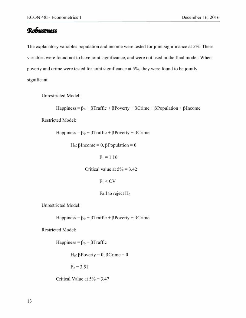
Robustness

The explanatory variables population and income were tested for joint significance at 5%. These

variables were found not to have joint significance, and were not used in the final model. When

poverty and crime were tested for joint significance at 5%, they were found to be jointly

significant.

Unrestricted Model:

Happiness = b0 + bTraffic + bPoverty + bCrime + bPopulation + bIncome

Restricted Model:

Happiness = b0 + bTraffic + bPoverty + bCrime

H0: bIncome = 0, bPopulation = 0

F1 = 1.16

Critical value at 5% = 3.42

F1 < CV

Fail to reject H0

Unrestricted Model:

Happiness = b0 + bTraffic + bPoverty + bCrime

Restricted Model:

Happiness = b0 + bTraffic

H0: bPoverty = 0, bCrime = 0

F2 = 3.51

Critical Value at 5% = 3.47


14

F2 > CV

Reject H0

Regression Results


15

Conclusions

The simple regression model I performed showed that traffic, as measured by total delay

per year in hours by city, and happiness, as determined from self-reported survey data, do in fact

share a statistically significant negative correlation. With data from the National Bureau of

Economic Research on subjective well-being and "Worst Corridor" analysis on traffic delay,

annually provided by INRIX, I was able to construct a sample size of 27 major metropolitan cities

in the United States. The magnitude of this correlation is quite small relative to the range of

possible happiness values, so it appears that traffic delay does not play a large role on perceived

happiness.

The multiple regression analyses show that while traffic is a factor in determining people's

happiness, it is not a major factor. This analysis provides evidence to support the claim that time

spent in traffic only decreases happiness on a local time scale. Over a longer time-scale, it is

possible that residents of high traffic cities adapt to the level of traffic and it no longer affects their

happiness. A correlation exists between traffic and happiness, but this small correlation does not

provide enough evidence that traffic has a large effect on a cities happiness levels. More research is

needed to determine why short term differences in traffic measurably effect a person’s happiness

but variations across space and long durations of time do not.

The goal of this research was to provide further insight into the relationship between

happiness and local levels of traffic. Data which encompasses more cities, including cities outside

of the United States, would be ideal to provide greater insight into the specific effects of local

traffic levels across cultures and national boundaries. Insight into the relative effects of other

independent variables, such as crime, weather, and income per capita, will be deduced from the


16

results of the multiple regression model and provide further insight into what other factors may be

at play. If in fact traffic does not play a large role on the happiness of individuals, cities might take

advantage of this insight to focus efforts on improving those factors which have greater effects on

subjective well-being.

These results could be improved by adding additional cities to my dataset, especially those

in Europe and Asia. The data I used was entirely comprised of US cities. This would seem like a

good thing because it is one way to hold culture constant, however culture varies widely across the

United States, so this supposed gain is actually nonexistent. Therefore, incorporating other cities

into my data could be a good way to increase the robustness of my findings. If it is shown that

European cities or Asian cities have higher correlations between traffic and happiness, my

conclusion that happiness has a very small negative effect on traffic will have to be reevaluated.

More data points, if they confirm the results from the United States, would increase the robustness

of my results and allow certainty in the fact that average traffic does not have a strong effect on

average happiness.


17

Appendix A: STATA Results

Simple Regression Results

Multiple Regression Results


18

References

Anderson, M., Lu, F., Zhang, Y., Yang, J., & Qin, P. (2016, October). Superstitions, Street Traffic, and

Subjective Well-Being. Journal of Public Economics, 142, 1-10. doi:10.3386/w21551

Glaeser, E. L., Gottlieb, J. D., & Ziv, O. (2016). Unhappy Cities. Journal of Labor Economics, 34(S2).

doi:10.1086/684044

Héritier, H., Vienneau, D., Frei, P., Eze, I., Brink, M., Probst-Hensch, N., & Röösli, M. (2014). The

Association between Road Traffic Noise Exposure, Annoyance and Health-Related Quality of Life

(HRQOL). International Journal of Environmental Research and Public Health, 11(12), 12652-12667.

doi:10.3390/ijerph111212652

INRIX 2015 Traffic Scorecard - INRIX. (2016). Retrieved October, 2016, from

http://inrix.com/scorecard/ONS. (n.d.). Commuting and Personal Well-being. UK Office of National

Statistics. Retrieved October, 2016.

US Census Bureau. (n.d.). Census.gov. Retrieved November 15, 2016, from http://www.census.gov/

Documents

Final draft Project(485)