NAVAL POSTGRADUATE SCHOOL Monterey, California

THESIS

Approved for public release; distribution is unlimited

DETECTION OF BINARY PHASE-SHIFT KEYING SIGNAL IN MULTIPATH PROPAGATION

by

Du San Jung

June 2002

Thesis Advisor: Charles W. Therrien Second Reader: Murali Tummala

THIS PAGE INTENTIONALLY LEFT BLANK

i

REPORT DOCUMENTATION PAGE Form Approved OMB No. 0704-0188 Public reporting burden for this collection of information is estimated to average 1 hour per response, including the time for reviewing instruction, searching existing data sources, gathering and maintaining the data needed, and completing and reviewing the collection of information. Send comments regarding this burden estimate or any other aspect of this collection of information, including suggestions for reducing this burden, to Washington headquarters Services, Directorate for Information Operations and Reports, 1215 Jefferson Davis Highway, Suite 1204, Arlington, VA 22202-4302, and to the Office of Management and Budget, Paperwork Reduction Project (0704-0188) Washington DC 20503. 1. AGENCY USE ONLY (Leave blank)

2. REPORT DATE June 2002

3. REPORT TYPE AND DATES COVERED Master’s Thesis

4. TITLE AND SUBTITLE: Detection of Binary Phase-Shift Keying Signal in Multipath Propagation 6. AUTHOR(S) Jung, Du San

5. FUNDING NUMBERS

7. PERFORMING ORGANIZATION NAME(S) AND ADDRESS(ES) Naval Postgraduate School Monterey, CA 93943-5000

8. PERFORMING ORGANIZATION REPORT NUMBER

9. SPONSORING /MONITORING AGENCY NAME(S) AND ADDRESS(ES) N/A

10. SPONSORING/MONITORING AGENCY REPORT NUMBER

11. SUPPLEMENTARY NOTES The views expressed in this thesis are those of the author and do not reflect the official policy or position of the Department of Defense or the U.S. Government. 12a. DISTRIBUTION / AVAILABILITY STATEMENT Approved for public release; distribution unlimited

12b. DISTRIBUTION CODE

13. ABSTRACT (maximum 200 words) Time-varying dispersion and multipath propagation in a shallow underwater environment causes intersymbol

interference in underwater communication. This thesis investigates a mitigation procedure for communication using a Binary

Phase-Shift Keying (BPSK) signal. The method employed uses the time-reversed ocean impulse response to mitigate the

degradation of the bit error rate performance. All results were achieved by the use of computer simulation of typical shallow

water environments.

15. NUMBER OF PAGES

105

14. SUBJECT TERMS Binary Phase-Shift Keying, underwater acoustics, acoustic communication, underwater communication, BPSK, MMPE, parabolic equation

16. PRICE CODE

17. SECURITY CLASSIFICATION OF REPORT

Unclassified

18. SECURITY CLASSIFICATION OF THIS PAGE

Unclassified

19. SECURITY CLASSIFICATION OF ABSTRACT

Unclassified

20. LIMITATION OF ABSTRACT

UL

NSN 7540-01-280-5500 Standard Form 298 (Rev. 2-89) Prescribed by ANSI Std. 239-18

ii

THIS PAGE INTENTIONALLY LEFT BLANK

iii

Approved for public release; distribution is unlimited

DETECTION OF BINARY PHASE-SHIFT KEYING SIGNAL IN MULTIPATH PROPAGATION

Du San Jung Lieutenant, Korean Navy

B.S., Republic of Korea Naval Academy, 1993

Submitted in partial fulfillment of the requirements for the degree of

MASTER OF SCIENCE IN ENGINEERING ACOUSTICS

from the

NAVAL POSTGRADUATE SCHOOL June 2002

Author: Du San Jung

Approved by: Charles W. Therrien, Thesis Advisor

Murali Tummala, Second Reader

Kevin B. Smith, Chairman Engineering Acoustics Academic Committee

iv

THIS PAGE INTENTIONALLY LEFT BLANK

v

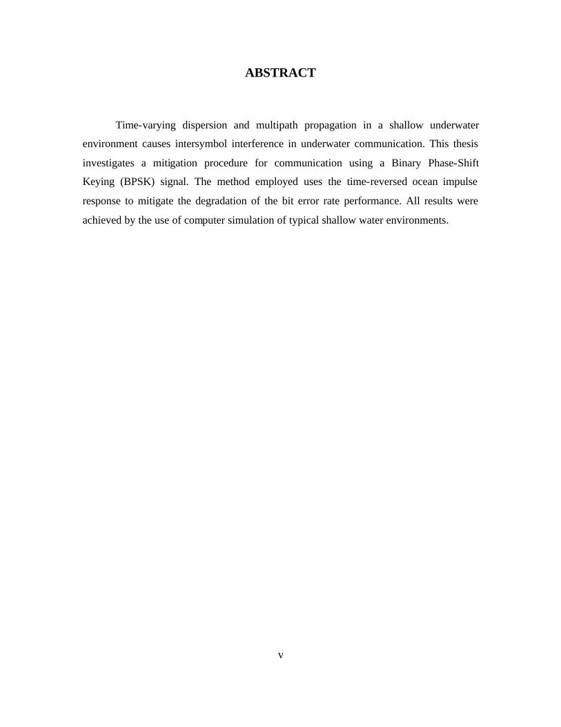
ABSTRACT Time-varying dispersion and multipath propagation in a shallow underwater

environment causes intersymbol interference in underwater communication. This thesis

investigates a mitigation procedure for communication using a Binary Phase-Shift

Keying (BPSK) signal. The method employed uses the time-reversed ocean impulse

response to mitigate the degradation of the bit error rate performance. All results were

achieved by the use of computer simulation of typical shallow water environments.

vi

THIS PAGE INTENTIONALLY LEFT BLANK

vii

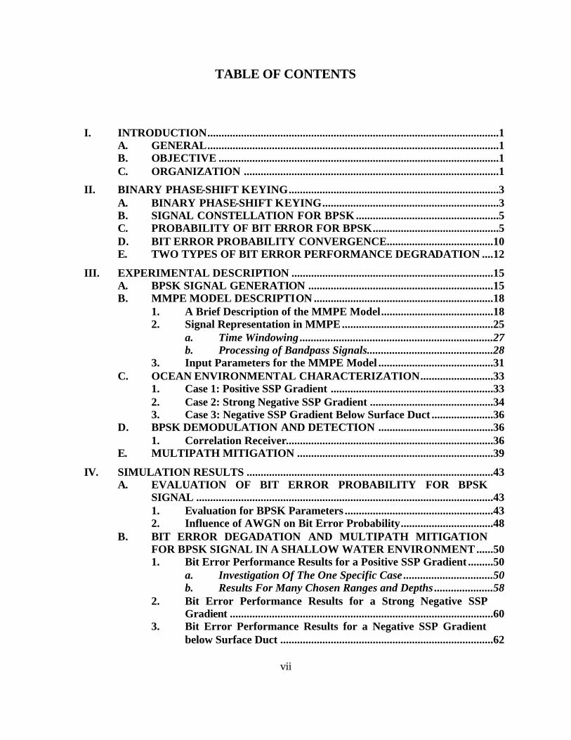
TABLE OF CONTENTS

I. INTRODUCTION........................................................................................................1 A. GENERAL........................................................................................................1 B. OBJECTIVE ....................................................................................................1 C. ORGANIZATION ...........................................................................................1

II. BINARY PHASE-SHIFT KEYING...........................................................................3 A. BINARY PHASE-SHIFT KEYING...............................................................3 B. SIGNAL CONSTELLATION FOR BPSK ...................................................5 C. PROBABILITY OF BIT ERROR FOR BPSK.............................................5 D. BIT ERROR PROBABILITY CONVERGENCE......................................10 E. TWO TYPES OF BIT ERROR PERFORMANCE DEGRADATION ....12

III. EXPERIMENTAL DESCRIPTION ........................................................................15 A. BPSK SIGNAL GENERATION ..................................................................15 B. MMPE MODEL DESCRIPTION ................................................................18

1. A Brief Description of the MMPE Model........................................18 2. Signal Representation in MMPE......................................................25

a. Time Windowing .....................................................................27 b. Processing of Bandpass Signals.............................................28

3. Input Parameters for the MMPE Model .........................................31 C. OCEAN ENVIRONMENTAL CHARACTERIZATION..........................33

1. Case 1: Positive SSP Gradient ..........................................................33 2. Case 2: Strong Negative SSP Gradient ............................................34 3. Case 3: Negative SSP Gradient Below Surface Duct ......................36

D. BPSK DEMODULATION AND DETECTION .........................................36 1. Correlation Receiver..........................................................................36

E. MULTIPATH MITIGATION ......................................................................39

IV. SIMULATION RESULTS ........................................................................................43 A. EVALUATION OF BIT ERROR PROBABILITY FOR BPSK

SIGNAL ..........................................................................................................43 1. Evaluation for BPSK Parameters .....................................................43 2. Influence of AWGN on Bit Error Probability.................................48

B. BIT ERROR DEGADATION AND MULTIPATH MITIGATION FOR BPSK SIGNAL IN A SHALLOW WATER ENVIRONMENT ......50 1. Bit Error Performance Results for a Positive SSP Gradient .........50

a. Investigation Of The One Specific Case ................................50 b. Results For Many Chosen Ranges and Depths .....................58

2. Bit Error Performance Results for a Strong Negative SSP Gradient ..............................................................................................60

3. Bit Error Performance Results for a Negative SSP Gradient below Surface Duct ............................................................................62

viii

V. CONCLUSIONS AND RECOMMENDATIONS...................................................65 A. CONCLUSIONS ............................................................................................65 B. RECOMMENDATIONS...............................................................................65

APPENDIX A. MMPE INPUT FILES FOR THREE DIFFERENT OCEAN ENVIRONMENTAL CASES ...................................................................................67 A. MMPE INPUT FILES FOR POSITIVE SSP GRADIENT.......................67

1. pefiles.inp File of the Main Input File .....................................67 2. pesrc.inp File of the Source Data................................................67 3. pessp.inp File of the Environmental Data ..................................68 4. pebath.inp File of the Environmental Data ...............................68 5. pebotprop.inp File of the Environmental Data ........................69 6. pedbath.inp File of the Environmental Data .............................69 7. pefiles.inp File of the Environmental Data .............................69

B. MMPE INPUT FILES FOR STRONG NEGATIVE SSP GRADIENT...70 1. pefiles.inp File of the Main Input File .....................................70 2. pessp.inp File of the Environmental Data ..................................70

C. MMPE INPUT FILES FOR NEGATIVE SSP GRADIENT BELOW SURFACE DUCT ..........................................................................................71 1. pefiles.inp File of the Main Input File .....................................71 2. pessp.inp File of the Environmental Data ..................................71

APPENDIX B. DETAILED SIGNAL PROCESSING STEPS.........................................73 A. RANDOM BINARY DATA GENERATION..............................................73 B. FILTERING ...................................................................................................74 C. GENERATION OF BPSK SIGNAL............................................................74 D. DEMODULATION OF BPSK SIGNAL, FILTERING.............................75 E. BER COUNTING ..........................................................................................76

APPENDIX C. COMPLETE PROCEDURES TO GENERATE THE PASSBAND OCEAN IMPULSE RESPONSE AND FREQUENCY RESPONSE FROM THE MMPE MODEL ...............................................................................................79 A. MODIFIED OCEAN FREQUENCY RESPONSE AND OCEAN

IMPULSE RESPONSE FROM MMPE MODEL ......................................79 B. BASEBAND OCEAN IMPULSE RESPONSE BY PADDING ZEROS ..79 C. FILTERING AND PRE-ENVELOPE OF THE OCEAN IMPULSE

RESPONSE ....................................................................................................81 D. PASSBAND OCEAN IMPULSE RESPONSE............................................82

LIST OF REFERENCES ......................................................................................................83

INITIAL DISTRIBUTION LIST.........................................................................................85

ix

LIST OF FIGURES

Figure 2.1. BPSK Signal in the Time Domain. ....................................................................3 Figure 2.2. BPSK Signal in Frequency Domain. .................................................................4 Figure 2.3. Signal Constellation for BPSK. .........................................................................5 Figure 2.4. Conditional Probability Density Functions: ( )1p z s , ( )2p z s .........................8

Figure 2.5. General Shape of the ΒΡ versus οNbΕ Curve................................................11 Figure 2.6. (a) Loss in οNbΕ . (b) Irreducible ΒΡ Caused by Distortion. .......................13 Figure 3.1. BPSK Signal Generation. .................................................................................15 Figure 3.2. Three Stages to Extract Ocean Response from MMPE Model. .......................18 Figure 3.3. Pulse Arriving after Propagation Delay τ .......................................................26 Figure 3.4. Spectrum of Bandpass Signal. .........................................................................27 Figure 3.5 Spectrum of a Complex Valued Lowpass Signal Corresponding to

Bandpass Signal of Figure 3.4. ........................................................................29 Figure 3.6. pefiles.inp File of the Main Input File....................................................31 Figure 3.7. pesrc.inp File of the Source Data. .............................................................32 Figure 3.8. pessp.inp File of the Environmental Data. ................................................33 Figure 3.9. (a) Positive SSP (b) Sound Propagation at Frequency 400 Hz, Source 5 m...34 Figure 3.10. (a) Negative SSP (b) Sound Propagation at Frequency 400 Hz, Source 30

m.......................................................................................................................35 Figure 3.11. (a) SSP (b) Sound Propagation at Frequency 400 Hz, Source 5 m. ...............36 Figure 3.12. Two Basic Steps in the Demodulation/Detection of the Received Signal. ......37 Figure 3.13. Correlator Receiver. .........................................................................................38 Figure 3.14 Multipath Mitigation for the Distorted Signal in Underwater Environment. ..40 Figure 4.1. The Power Spectral Density for BPSK Signal.................................................44 Figure 4.2. General FIR Filter (Hamming Window Design). ............................................46 Figure 4.3. Frequency Response for BPSK Signal Sampled by Null-to-null

Bandwidth. .......................................................................................................47 Figure 4.4. Frequency Response for BPSK Signal Sampled by Power Bandwidth. ..........47 Figure 4.5. BER versus SNR(dB). ........................................................................................49 Figure 4.6. BPSK Signal in Time Domain and Frequency Domain. .................................51 Figure 4.7. Passband Ocean Frequency Response (Magnitude and Phase) and Ocean

Impulse Response. ...........................................................................................52 Figure 4.8. Received Signal in Time Domain and Frequency Domain. ............................53 Figure 4.9. Comparison of Recovered Binary Data with Transmitted Binary Data for

the Received Signal. .........................................................................................54 Figure 4.10. Time Reversed Ocean Frequency Response (Magnitude and Phase) and

Ocean Impulse Response. ................................................................................55 Figure 4.11. Mitigated Ocean Impulse Response and Frequency Response........................56 Figure 4.12. Mitigated Signal in Time and Frequency Domain...........................................57 Figure 4.13. Comparison of Recovered Binary Data with Transmitted Binary Data for

Mitigated Signal Showing Zero Error..............................................................57

x

Figure 4.14. Bit Error Performance for Received Signal at Chosen Depths 5 to 95 m and Ranges 0.5 to 9.5 km for a Positive SSP Gradient. ...................................59

Figure 4.15. Bit Error Performance for Mitigated Signal at Chosen Depths 5 to 95 m and Ranges 0.5 to 9.5 km for a Positive SSP Gradient. ...................................60

Figure 4.16. Bit Error Performance for Received Signal at Chosen Depths 5 to 95 m and Ranges 0.5 to 9.5 km for a Strong Negative SSP Gradient.......................61

Figure 4.17. Bit Error Performance for Mitigated Signal at Chosen Depths 5 to 95 m and Ranges 0.5 to 9.5 km for a Strong Negative SSP Gradient.......................62

Figure 4.18. Bit Error Performance for Received Signal at Chosen Depths 5 to 95 m and Ranges 0.5 to 9.5 km for a Negative SSP Gradient below Surface Duct. .................................................................................................................63

Figure 4.19. Bit Error Performance for Mitigated Signal at Chosen Depths 5 to 95 m and Ranges 0.5 to 9.5 km for a Negative SSP Gradient below Surface Duct. .................................................................................................................64

Figure B-1. Random Binary Data in Time Domain and Frequency Domain......................73 Figure B-2. Frequency Response of the FIR Filter and the Filtered Binary Data...............74 Figure B-3. BPSK Signal [ ]s n in Time Domain and Frequency Domain. ........................75

Figure B-4. Demodulated BPSK Signal [ ]y n in Frequency Domain. ...............................76 Figure B-5. Demodulated and Filtered BPSK Signal in Time and Frequency Domain. ....76 Figure B-6. Comparison between Recovered Binary Data and Transmitted Binary

Data. .................................................................................................................77 Figure C-1. Modified Ocean Frequency Response ( )'H f and Impulse Response

[ ]'h n . ..............................................................................................................80

Figure C-2. Baseband Ocean Frequency Response ( )oH f and Impulse Response

[ ]oh n ................................................................................................................80 Figure C-3. Frequency Response of FIR Filter and Filtered Baseband Ocean

Frequency Response. .......................................................................................81 Figure C-4. Pre-Envelope Ocean Frequency Response ( )pH f . .......................................82

Figure C-5. Passband Ocean Frequency Response ( )bH f ................................................82

xi

LIST OF VARIABLES

AWGN additive white Gaussian noise cA sinusoidal carrier amplitude

{ }na message data or a set of random variables with 1na = ± BPSK binary phase-shift keying

)(tb random binary signal )( fBT Fourier transform of the truncated signal, )(tbT

)( fB Fourier transform of a random binary signal )(tbT truncated signal of )(tb

[ ]b n discrete random binary data

[ ]fb n filtered random binary data

( )c xr

sound speed

0c reference sound speed DFT Discrete Fourier Transform

[ ]d n cosine demodulating signal

bΕ average energy per bit

cf center frequency or carrier frequency

sf sampling frequency '

sf up-sampling frequency [ ]⋅FT Fourier transform

[ ]1FT − ⋅ inverse Fourier transform

)( bntg Τ− rectangular pulse with bit time duration, bT )( fG Fourier transform for a rectangular pulse

xii

)(th ocean impulse response

( )h t− time-reversed ocean impulse response )( fH ocean frequency response

'( )H f modified ocean frequency response

[ ]h n discrete ocean impulse response

[ ]'h n modified ocean impulse response

[ ]bh n passband ocean impulse response

( )bH f passband ocean frequency response

[ ]th n time-reversed ocean impulse response

[ ]mh n mitigated ocean impulse response

[ ]h nο baseband ocean impulse response

( )H fο baseband ocean frequency response

[ ]ph n pre-envelope of passband ocean impulse response

( )pH f pre-envelope of passband ocean frequency response

[ ]LPFh n FIR lowpass filter ISI intersymbol interference I interpolation factor

[ ]k n cosine modulating signal

kο reference wavenumber L number of time and frequency samples used in the transform l index of refraction

( )n t additive white Gaussian noise nο noise component of the output of the correlator

bitN number of bits in the transmitted binary data 2οN two-sided noise power spectral density

οN noise power spectral density N noise power

sbN number of samples per bit

xiii

ΒΡ probability of bit error

ΕΡ probability of symbol error

( )i jP s s conditional probabilities

( )jp z s conditional probability density function

( )isP prior probability of the symbols pdf probability density function PSD power spectral density

)( fPb PSD for a random binary signal with a rectangular pulse )( fPs PSD of BPSK signal

( )txp , acoustic pressure as a function of position x and time t

( )BPSKP f+ single-sided power spectral density

( )q t received signal

[ ]q n discrete time received signal

( )⋅Q complementary error function r range R bit rate ( )sec/bits

BPSKs BPSK signal set )(ts BPSK signal

( )bs t continuous-time real bandpass signal

[ ]s n discrete time BPSK signal

( )ps t “in-phase” modulation components

( )qs t “quadrature” modulation components

( )s t% complex envelope of BPSK signal

( )s t$ mitigated signal

[ ]s n$ discrete time mitigated signal

[ ]S k DFT coefficient of [ ]s n S signal power SNR average signal power to average noise power ratio

xiv

SNR (dB) SNR in decibels ( )txS , sound source distribution as a function of position x and time t

( )S f% frequency spectrum of a complex valued low-pass signal

( )bS f frequency spectrum of bandpass signal

t∆ sampling interval bΤ bit time duration or symbol time duration

t time 't reduced time

TL transmission loss

iv signal component of the output of the correlator

( )1w t single waveform for the BPSK signal set W bandwidth ω digital frequency x spatial position at which the pressure signal is measured

( )y t recovered signal

[ ]y n discrete time recovered signal

( )bz T correlator output or decision statistic at bit time duration bT z depth

ογ decision threshold

2οσ white Gaussian noise variance

)(tφ sinusoidal carrier

xv

)( fΦ Fourier transform of a sinusoidal carrier )(tφ

( )⋅δ delta function

( ), , ,r z fϕΨ PE field function τ gross propagation delay

οτ propagation delay ϕ azimuthal angle

( )i tΘ phase term of transmitted BPSK signal

xvi

THIS PAGE INTENTIONALLY LEFT BLANK

xvii

ACKNOWLEDGMENTS I wish to give recognition to:

My thesis advisor, Professor Charles W. Therrien, for his time and support in past

one year. His expertise advice, directions and great help were an enormous support to me

in achieving this thesis.

My second reader, Professor Murali Tummala, for his time and help. Especially

discussing the results with him was a great help to me.

Professor, Kevin B. Smith, for valuable comments

My wife, Sug Hyun Park, for her love, devotion and encouragement throughout

my tour at the Naval Postgraduate School. Thanks to her outstanding skills as a mother

and a wife. I will always love you, perhaps some days more than others.

My two sons, Sung Yeop and Sung Moon. Although they are probably too young

to realize, they constantly kept my daily life in the correct perspective.

My parents, Tae Young Jung and Cha Soon Cho, for their never-ending love and

encouragement for me.

My country and Republic of Korea Navy for sending me to NPS to have this

education and opportunity. NPS not only gave me a good technical knowledge but also

awarded me a different way of looking at life.

xviii

THIS PAGE INTENTIONALLY LEFT BLANK

1

I. INTRODUCTION

A. GENERAL

The underwater environment is the most challenging region of the battle space in

which to communicate effectively. Sound propagation in an underwater communication

channel becomes a very difficult task due to numerous constraints and limitations

imposed by the nature of the medium and the environment. The most important

characteristic s of the underwater environment that put limitations on the performance of

underwater communication are dispersion caused by the spatial and temperal variability

and multipath propagation. Multipath propagation produces intersymbol interference

(ISI) and severe degradation of the bit error performance in digital communication. The

specific investigation in this thesis is the demodulation of Binary Phase-Shift Keying

(BPSK) in three different shallow water ocean acoustic channels.

B. OBJECTIVE

The objective of this thesis was to study the possibility of using the time-reversed

ocean impulse response prior to the demodulation of a BPSK signal to mitigate the

degradation of the bit error performance in multipath propagation. The thesis evaluates

the bit error performance of the mitigated signal compared to the bit error performance of

the received signal distorted by the intersymbol interference in three different ocean

environments in the absence of noise.

C. ORGANIZATION

The remainder of this thesis is organized as follows. Chapter II gives the general

theory related to BPSK binary communication. This describes the definition, waveform

and constellation of the BPSK signal, the theoretical convergence of the bit error

probability, and two types of the bit error degradation factors. Chapter III describes the

experiments and simulation procedure used in this thesis. This includes a time-domain

and frequency-domain BPSK representation, Power Spectral Density (PSD) for BPSK, a

description of the Monterey-Miami Parabolic Equation (MMPE) model, the ocean

impulse response extraction from MMPE model, BPSK demodulation and multipath

mitigation. Chapter IV provides the main results of the simulation. Included in the results

are the evaluation for the bit error performance of the BPSK signal, bit error degradation

2

and multipath mitigation for BPSK signal in three different shallow water acoustic

channels.

3

II. BINARY PHASE-SHIFT KEYING

This chapter describes the general theory related to binary phase-shift keying

(BPSK). First, the definition, waveform and its constellation for BPSK modulation are

explained. Next, as an important criterion of performance in digital communication, the

probability of bit error is defined and the theoretical convergence of the bit error

probability is described. Finally, two types of the bit error degradation factors are

presented.

A. BINARY PHASE-SHIFT KEYING

In binary phase-shift keying (BPSK), the phase of a constant-amplitude carrier

signal is switched between two values according to the two possible “messages” 1m and

2m corresponding to binary 1 and 0, respectively. Normally, the two phases are separated

by 180 degrees. If the sinusoidal carrier has amplitude cΑ , then the average energy per bit

is bΕ =21 2

cΑ bΤ where bΤ is the bit time duration, and the transmitted BPSK signal can

be represented as:

[ ]2( ) cos 2 ( )b

i c ib

s t f t tπΕ

= + ΘΤ

0

1,2bt

i≤ ≤ Τ

= ( )1.2

where the phase term, )(tiΘ , will have two discrete values, given by 1Θ =0 and 2 πΘ = .

In other words, in BPSK modulation, the modulating data signal shifts the phase of the

waveform is (t) to one of two states, either zero or (180 )π ° . Instead of using a

rectangular shaped pulse as shown in Figure 2.1, we can use non-rectangular shaped

pulses by applying hanning, hamming, and Gaussian windows. However, we shall adhere

to the simplest case of a rectangular pulse in this thesis.

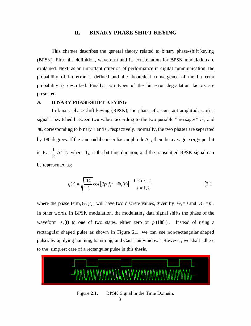
Figure 2.1. BPSK Signal in the Time Domain.

4

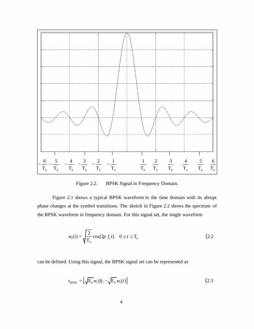
Figure 2.2. BPSK Signal in Frequency Domain.

Figure 2.1 shows a typical BPSK waveform in the time domain with its abrupt

phase changes at the symbol transitions. The sketch in Figure 2.2 shows the spectrum of

the BPSK waveform in frequency domain. For this signal set, the single waveform

1

2( ) cos(2 )c

b

w t f tπ=Τ

bt Τ≤≤0 ( )2.2

can be defined. Using this signal, the BPSK signal set can be represented as

{ }1 1( ) , ( )BPSK b bs w t w t= Ε − Ε ( )3.2

1

bΤ2

bΤ6

bΤ1

b

−Τ

2

b

−Τ

6

b

−Τ

3

bΤ4

bΤ5

bΤ4

b

−Τ

3

b

−Τ

5

b

−Τ

/ ■ "T"" r

1 1 /

/A f\ \ i | \r -/

i i i i

5

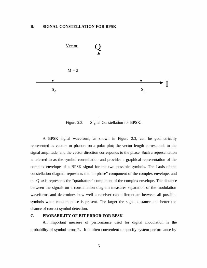
B. SIGNAL CONSTELLATION FOR BPSK

Vector

M = 2

S1 S2

I

Q

••

Figure 2.3. Signal Constellation for BPSK.

A BPSK signal waveform, as shown in Figure 2.3, can be geometrically

represented as vectors or phasors on a polar plot; the vector length corresponds to the

signal amplitude, and the vector direction corresponds to the phase. Such a representation

is referred to as the symbol constellation and provides a graphical representation of the

complex envelope of a BPSK signal for the two possible symbols. The I-axis of the

constellation diagram represents the “in-phase” component of the complex envelope, and

the Q-axis represents the “quadrature” component of the complex envelope. The distance

between the signals on a constellation diagram measures separation of the modulation

waveforms and determines how well a receiver can differentiate between all possible

symbols when random noise is present. The larger the signal distance, the better the

chance of correct symbol detection.

C. PROBABILITY OF BIT ERROR FOR BPSK

An important measure of performance used for digital modulation is the

probability of symbol error, ΕΡ . It is often convenient to specify system performance by

6

the probability of bit error ΒΡ , even when decisions are made on the basis of symbols

rather than bits. The relationship between ΒΡ and ΕΡ for orthogonal signaling is:

2logΕ

ΒΡ

Ρ =Μ

( )4.2

where M is the number of symbols.

For BPSK modulation (M=2), the symbol error probability is equal to the bit error

probability. When the signals are assumed equally likely and signal )(tsi ( )2,1=i is

transmitted, the received signal, ( )q t , is equal to )()( tntsi + , where )(tn is modeled as

additive white Gaussian noise (AWGN). The antipodal signals (signals of equal

amplitude and opposite polarity) )(1 ts and )(2 ts are [cf. Eq. ( )3.2 ]:

1 1( ) ( )bs t w t= Ε 0 bt≤ ≤ Τ ( )5.2

2 1( ) ( )bs t w t= − Ε 0 bt≤ ≤ Τ ( )6.2

The detection and demodulation of the received signal involves a correlation with

each of the antipodal signals, as explained in Chapter 3. At the end of each symbol

duration bΤ , the output of the correlator yields a sample ( )bz Τ , called the detection

statistic given by

( ) ( ) ( )b i b bz v nοΤ = Τ + Τ 1,2i = ( )2.7

where ( )i bv Τ is the desired signal component and ( )bnο Τ is the noise component. The

noise component is a zero mean Gaussian random variable, and thus ( )bz Τ is a Gaussian

7

random variable with a mean of either 1v or 2v depending on whether ( )1s t or ( )2s t was

sent.

The decision stage of the detector will choose the )(tsi with the largest correlator

output )(tzi , or in this case of equal-energy antipodal signals, the detector, using the

decision rules, decides:

)(1 ts if ( )bz ογΤ > ( )2.8

)(2 ts otherwise ( )2.9

where ογ denotes the decision threshold (equal to 0 for equally probable antipodal

signals) and ( )bz Τ is the correlator output at time bΤ . Two types of detection errors can

be made. The first type of error takes place if )(1 ts is transmitted but the detector

measures a negative value for ( )bz Τ and decides (incorrectly) that signal )(2 ts was sent.

The second type of error takes place if signal )(2 ts is transmitted but the detector

measures a positive value for ( )bz Τ and decides (again incorrectly) that signal )(1 ts was

sent. Therefore, the probability of bit error, ΒΡ , is the sum:

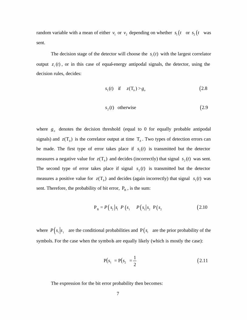
( ) ( ) ( ) ( )2 1 1 1 2 2P s s P s P s s sΒΡ = + Ρ ( )2.10

where ( )i jP s s are the conditional probabilities and ( )isΡ are the prior probability of the

symbols. For the case when the symbols are equally likely (which is mostly the case):

( ) ( )21

21 =Ρ=Ρ ss ( )2.11

The expression for the bit error probability then becomes:

8

( ) ( )2 1 1 2

1 12 2

P s s P s sΒΡ = + ( )2.12

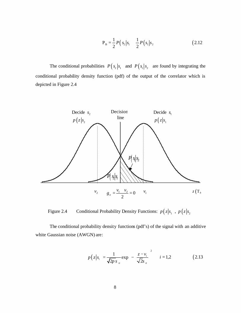
The conditional probabilities ( )2 1P s s and ( )1 2P s s are found by integrating the

conditional probability density function (pdf) of the output of the correlator which is

depicted in Figure 2.4

Figure 2.4 Conditional Probability Density Functions: ( )1p z s , ( )2p z s

The conditional probability density functions (pdf’s) of the signal with an additive

white Gaussian noise (AWGN) are:

( )2

1exp

2 2i

i

z vp z s

ο οπ σ σ

− = − 2,1=i ( )2.13

1 2 02

v vογ

+= =2v 1v ( )bz Τ

Decide 2s

( )2p z s

Decide 1s

( )1p z s

Decision line

( )1 2P s s

( )2 1P s s

9

i.e., the conditional pdf’s ( )ip z s ( )2,1=i are Gaussian with mean value iv , and

variance 2οσ where 2

οσ corresponds to the noise variance at the output of the correlator.

Because of the symmetry of ( )ip z s , the bit error probability of Eq. ( )2.12 reduces to:

( ) ( )2 1 1 2P s s P s sΒΡ = = ( )2.14

Thus, the probability of a BPSK bit error ΒΡ is numerically equal to the area

under the “tail” of either pdf ( )1p z s or ( )2p z s that falls on the incorrect side of the

threshold. We can therefore compute ΒΡ by either integrating ( )1p z s between the limits

∞− and ογ or by integrating ( )2szp between the limits ογ and ∞ , where

ογ = ( )1 2 2v v+ is the optimum threshold. Hence,

( )2p z s dzογ

∞

ΒΡ = ∫ ( )2.15

Using Eq. ( )2.13 , the probability of bit error for BPSK is:

2

21 1exp

22z v

dzο ογ ο

σσ π

∞

Β

− Ρ = −

∫ ( )2.16

If we introduce 2z vu

οσ−

= and dzdu =οσ , the integral simplifies to

( )1 2

21 2

2

1exp

2 22v v

v vudu Q

ο οσ σπ

∞

Β−

−Ρ = − =

∫ ( )2.17

10

where ( )⋅Q is the complementary error function defined as:

duu

xQx∫∞

−=

2exp

2

1)(

2

π ( )2.18

For equal energy antipodal signaling, such as the BPSK format in Eq. (2.3), the

receiver output signal components are 1 bv = Ε when )(1 ts is sent and 2 bv = − Ε when

)(2 ts is sent. For AWGN, the noise variance 2οσ of the correlator output can be written

as 2οN , where 2οN is two-sided power spectral density of the noise. Thus, we can

rewrite probability of bit error as follows:

Ε=

−=Ρ ∫

∞

ΕΒ

οοπ N

Qduu b

Nb

22

exp21 2

2

( )2.19

D. BIT ERROR PROBABILITY CONVERGENCE

In digital communications, we more often use οNbΕ , a normalized version of

average signal power to average noise power ratio ( S N or SNR ), as a figure of merit.

bΕ is bit energy and can be described as signal power S times the bit time bT . οN is

noise power spectral density, and can be described as noise power N divided by

bandwidth W . Since the bit time and bit rate bR are reciprocal, we can replace bΤ with

bR1 and write

b b bST S RN N W N Wο

Ε= = ( )2.20

If we use R instead of bR to represent bits/sec, and we rewrite Equation ( )2.20

to emphasize that οNbΕ is just a version of S N normalized by bandwidth and bit rate,

we obtain:

11

=

ΕRW

NS

Nb

ο

( )2.21

One of the most important metrics of performance in a digital communication

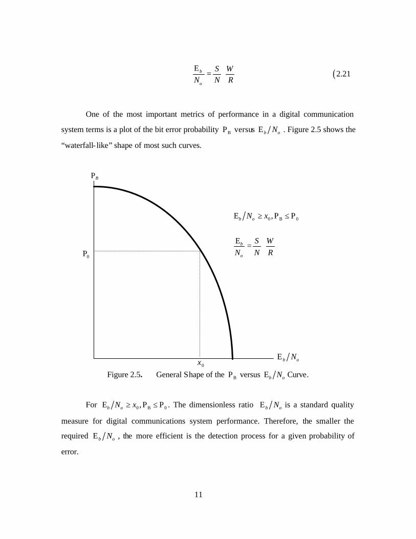
system terms is a plot of the bit error probability ΒΡ versus οNbΕ . Figure 2.5 shows the

“waterfall- like” shape of most such curves.

Figure 2.5. General Shape of the ΒΡ versus οNbΕ Curve.

For 0 0,b N xο ΒΕ ≥ Ρ ≤ Ρ . The dimensionless ratio οNbΕ is a standard quality

measure for digital communications system performance. Therefore, the smaller the

required οNbΕ , the more efficient is the detection process for a given probability of

error.

0 0,b

b

N x

S WN N R

ο

ο

ΒΕ ≥ Ρ ≤ Ρ

Ε = 0Ρ

0x οNbΕ

BΡ

or

12

To optimize (minimize) ΒΡ in the context of an AWGN channel and the receiver,

we need to select the optimum receiving filter and the optimum decision threshold. For

the binary case, the optimum decision threshold is ογ = ( )1 2 2v v+ and it was shown in

Equation ( )2.17 that this threshold results in ( )1 2 2Q v v οσΒΡ = − . Next, for

minimizing ΒΡ , it is necessary to maximize the argument of ( )xQ . Thus, we need to

maximize ( )1 2 2v v οσ− or equivalently, maximize

( )2

1 22

v vSNR

οσ−

= ( )2.22

where ( )1 2v v− is the difference of the desired signal components at the filter output at

time bt = Τ , and the square of this difference signal is the instantaneous power of the

difference signal. The SNR can also be maximized by minimizing οσ 2 ; however, 2οσ is

usually not under our control.

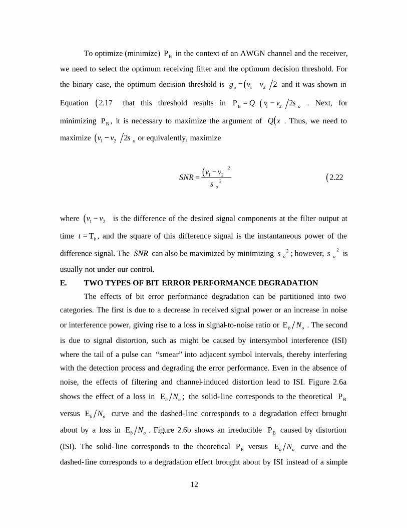
E. TWO TYPES OF BIT ERROR PERFORMANCE DEGRADATION

The effects of bit error performance degradation can be partitioned into two

categories. The first is due to a decrease in received signal power or an increase in noise

or interference power, giving rise to a loss in signal-to-noise ratio or οNbΕ . The second

is due to signal distortion, such as might be caused by intersymbol interference (ISI)

where the tail of a pulse can “smear” into adjacent symbol intervals, thereby interfering

with the detection process and degrading the error performance. Even in the absence of

noise, the effects of filtering and channel- induced distortion lead to ISI. Figure 2.6a

shows the effect of a loss in ;b NοΕ the solid- line corresponds to the theoretical ΒΡ

versus οNbΕ curve and the dashed- line corresponds to a degradation effect brought

about by a loss in οNbΕ . Figure 2.6b shows an irreducible ΒΡ caused by distortion

(ISI). The solid- line corresponds to the theoretical ΒΡ versus οNbΕ curve and the

dashed- line corresponds to a degradation effect brought about by ISI instead of a simple

13

loss in signal-to-noise ratio. The bit error rate in this case cannot further be reduced by

increasing the signal power.

Figure 2.6. (a) Loss in οNbΕ . (b) Irreducible ΒΡ Caused by Distortion.

)(dBNb οΕ

10 12

1

110−

210−

310−

410−

510−

ΒΡ

)(dBNb οΕ

10 12

1

110−

210−

310−

410−

510−

ΒΡ

Caused by distortion

14

THIS PAGE INTENTIONALLY LEFT BLANK

15

III. EXPERIMENTAL DESCRIPTION

In this chapter, we describe the experiments and simulation procedure used in this

thesis. First, as a part of BPSK signal generation, time-domain and frequency-domain

BPSK representations and Power Spectral Density (PSD) for BPSK are analytically

derived. Second, we describe the Monterey-Miami Parabolic Equation (MMPE) acoustic

simulation model and how to generate the ocean responses in the time-domain and

frequency-domain from the MMPE model. Third, we describe the ocean environment for

our simulations and the input data for the MMPE model. Finally, we present the results of

BPSK demodulation and multi-path mitigation.

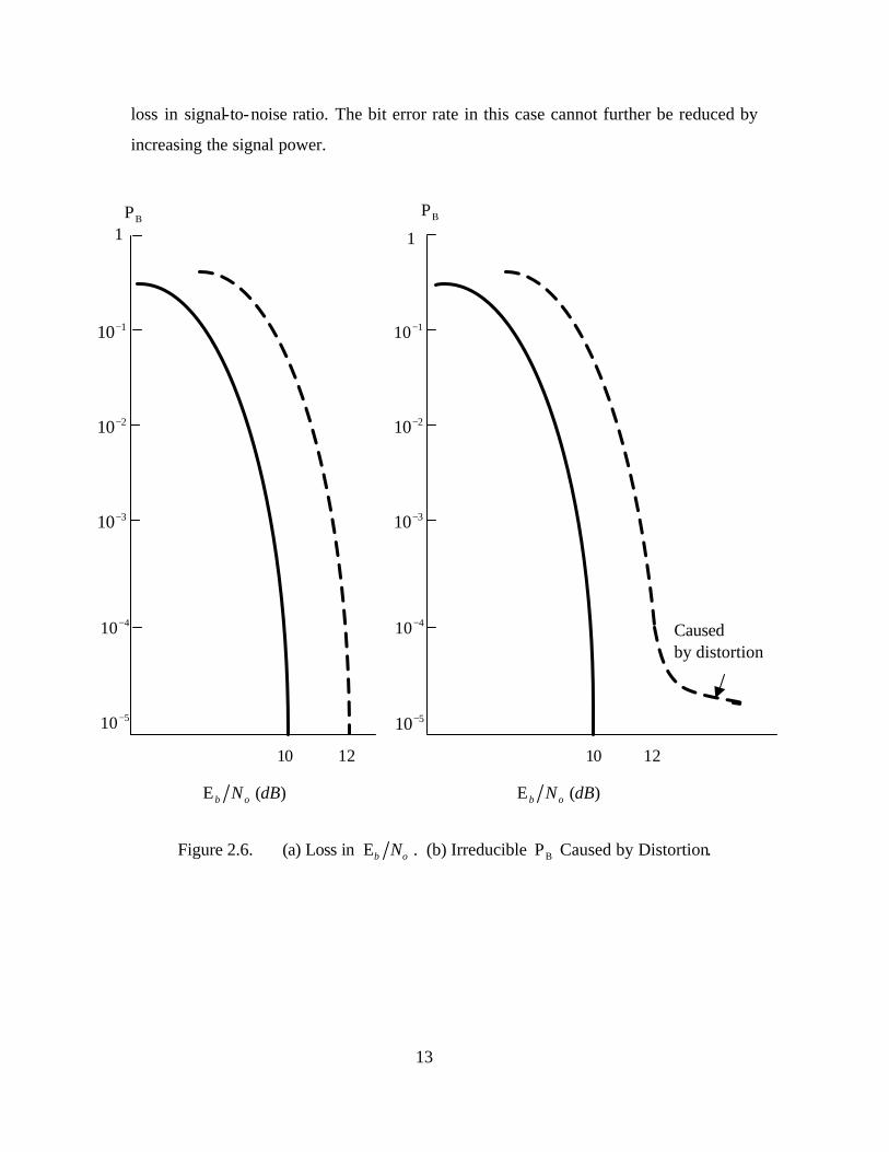
A. BPSK SIGNAL GENERATION

In Chapter II, we described the properties of BPSK. In this section, time-domain

and frequency-domain representations for the BPSK waveform are described and related

to the ocean impulse response, and the power spectral density of the received signal.

Figure 3.1 shows a diagram for BPSK signal generation. The quantity )(tb is a random

binary signal at baseband. The message data, { }na represent a set of random variables

with 1±=na and probabilities ( ) ( )21

11 =−=== nn aPaP . The function ( )bg t n− Τ is a

shaped pulse in general; however we will take it to be a rectangular pulse with bit time

duration, .bΤ The signal )(tφ is a sinusoidal carrier with center frequency cf and

amplitude cA . The output )(ts is the modulated BPSK signal.

Figure 3.1. BPSK Signal Generation.

( )( ) n bn

b t a g t n∞

=−∞

= − Τ∑ )()()( ttbts φ⋅=

Random binary signal BPSK signal

( )( ) cos 2c ct A f tφ π= Sinusoidal carrier

16

The Fourier transform for a rectangular pulse with amplitude one and bit duration

bΤ is given by:

( )2

2

2 sin( )( )

b

b

bb

b

j ft fG f g t e

fπ π

π

Τ−

Τ−

ΤΤ

Τ= =∫ ( )1.3

The Power Spectral Density (PSD) for a random binary signal, ( ),b t will be

evaluated by first truncating )(tb as follows:

( ) ( )n N

T n bn N

b t a g t n=

=−

= − Τ∑ , 2 2tο ο− Τ ≤ ≤ Τ ( )2.3

where )(tbT is the truncated signal and ( )2 1 2 .bNοΤ = + Τ The Fourier transform of the

truncated signal, ( ),Tb t is then,

[ ] ( )[ ] ∑∑−=

Τ−

−=

=Τ−==N

Nn

njn

N

NnbnTT

befGantgFTatbFTfB ω)()()(

∑−=

Τ−=N

Nn

njn

beafG ω)( ( )3.3

where the notation [ ]⋅FT represents the Fourier transform operation and ( )G f is the

resulting Fourier transform of ( )g t .

The PSD for the random signal )(tb can be defined by [Ref 3]

( ) 2

( ) limT

b

B fP f

ο οΤ →∞

= Τ

( )4.3

17

where ( )fBT represents the Fourier transform of the corresponding truncated signal and

the overbar represents statistical expectation. Upon substituting ( )3.3 into ( )4.3 , the PSD

of )(tb becomes

( )2

22 21 1 2 1( ) lim ( ) ( ) lim 1 limb

N Nj n

b nn N n N

NP f G f a e G f G f

ο ο ο

ω

ο ο ο

− Τ

Τ →∞ Τ →∞ Τ →∞=− =−

+ = = = Τ Τ Τ ∑ ∑

where we have assumed that the na are statistically independent. Now, using

( )2 1 2 bT Nο = + Τ , we obtain

( )

222 )sin(

)(1

1212

lim)()(

Τ

ΤΤ=

Τ=

Τ+

+=

∞→b

bb

bbNb f

ffG

NN

fGfPπ

π ( )5.3

where Eq. ( )1.3 has been used for )( fG . This is the PSD of the signal at “baseband.”

For the modulated BPSK signal we have

( )tfAtbts cc π2cos)()( = ( )6.3

The corresponding PSD is given by

( ) ( )cbc

cbc

s ffPA

ffPA

fP −++=44

)(22

( )7.3

(see Ref 3), where bP is the PSD of the baseband signal )(tb . Upon substituting ( )5.3

into ( )7.3 we obtain

18

( ) ( )[ ]222

4)( cc

bcs ffGffG

AfP −++

Τ=

( )

( )( )

( )

Τ−

Τ−+

Τ+

Τ+Τ=

222 sinsin4 bc

bc

bc

bcbc

ffff

ffffA

ππ

ππ

( )8.3

B. MMPE MODEL DESCRIPTION

The Parabolic Equation (PE) method was introduced into underwater acoustics in

the early 1970’s by Tappert [Ref 8]. The Monterey-Miami Parabolic Equation (MMPE)

model [Ref 9] is a numerical model to solve acoustic wave propagation problems in the

ocean using the PE method. The MMPE Model is used to compute the response at the

receiver location of a signal transmitted from a source and traveling through the ocean.

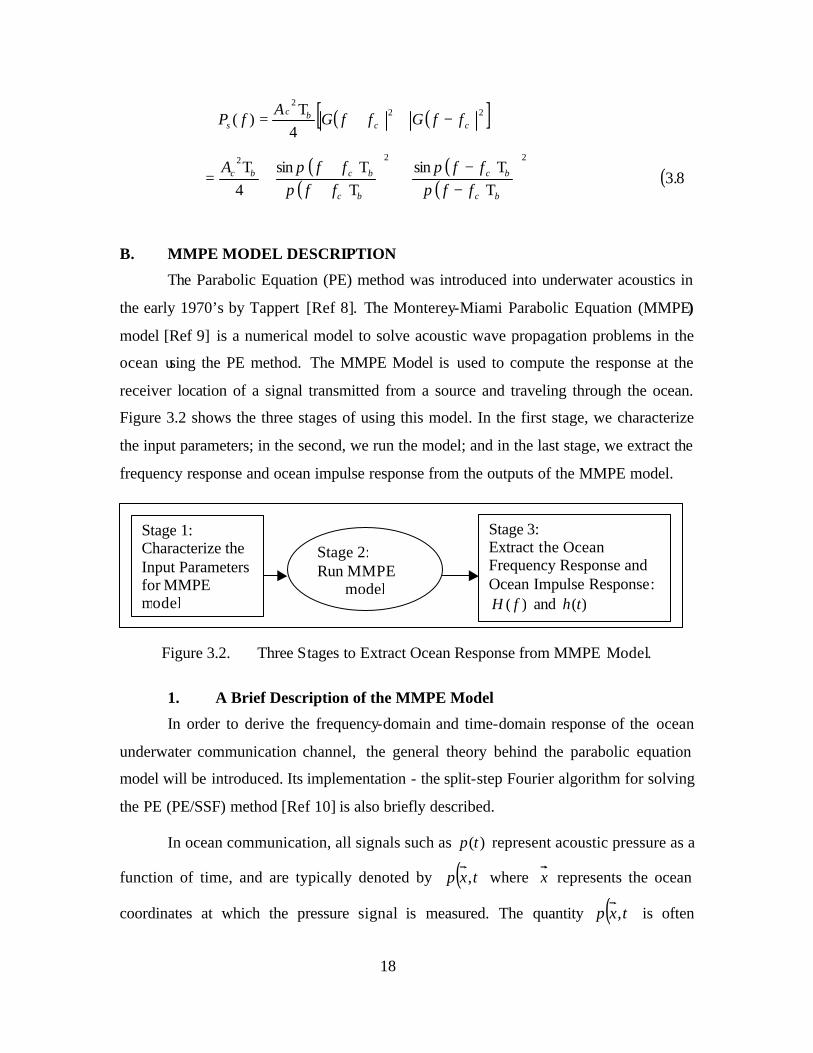
Figure 3.2 shows the three stages of using this model. In the first stage, we characterize

the input parameters; in the second, we run the model; and in the last stage, we extract the

frequency response and ocean impulse response from the outputs of the MMPE model.

Figure 3.2. Three Stages to Extract Ocean Response from MMPE Model.

1. A Brief Description of the MMPE Model

In order to derive the frequency-domain and time-domain response of the ocean

underwater communication channel, the general theory behind the parabolic equation

model will be introduced. Its implementation - the split-step Fourier algorithm for solving

the PE (PE/SSF) method [Ref 10] is also briefly described.

In ocean communication, all signals such as )(tp represent acoustic pressure as a

function of time, and are typically denoted by ( )txp , where x represents the ocean

coordinates at which the pressure signal is measured. The quantity ( )txp , is often

Stage 1:

Characterize the Input Parameters for MMPE model

Stage 2: Run MMPE

model

Stage 3: Extract the Ocean Frequency Response and Ocean Impulse Response:

)( fH and )(th

19

referred to as a space-time signal, since it is a function of the spatial parameters x and

time t . When measured at a fixed (receiver) location (say x = 1x ) it becomes a function

of time only. It is transformed into an electrical signal by an acoustic transducer or

hydrophone.

The inhomogeneous wave (Helmholtz) equation for the acoustic pressure ),( txp

in a medium with sound speed ( )c xr

and density ( )xρr

can be expressed as

( ) ( )( ) ( )

( ) ( )2

2 2

, ,1,

p x t p x tx S x t

tx c xρ

ρ

∇ ∂ ∇ ⋅ − = ∂

r rr r

r r ( )9.3

where ( ),S x tr

represents the sound source distribution as a function of both position x

and time t . In our application (as in most) there is a single source at a particular location

x xο=r r

. Hence ( )txS , is formally a spatial “impulse” at οx with time dependence

)(ts corresponding to the transmitted waveform.

The parabolic equation model is based on an approximation of the Helmholtz

wave equation in a cylindrical coordinate system. Because of the ocean’s relative

shallowness compared to horizontal propagation distance for the majority of

environments, it is well suited for a description in cylindrical coordinates.

The signals of interest in underwater communications such as BPSK have

complicated time dependence; thus analytical solution to the wave equation ( )9.3 would

be impossible. However the equation is linear, and a solution can be computed relatively

easily for sources that have time dependence of the form ftje π2 for a single frequency f .

Thus for a source with a time dependence of the form ftjAe π2 , the output at a point x = 1x

is dependent on f and can be written as ftj

xefH π2)(

1. This is referred to by people

working in ocean acoustics as a “time harmonic” solution to the wave equation. The

quantity )(1

fHx

is the ocean frequency reponse and its inverse Fourier transform is the

20

ocean impulse response (Green’s function). The time harmonic solution forms the basis

of computing the response due to a source with arbitrary time dependence by using

Fourier analysis/synthesis methods.

From this point forward the analysis will be carried out in discrete time. This is

appropriate since numerical techniques (i.e., the DFT) are used to perform the

computations in both the time and frequency domains. We focus first on the analysis of

low-pass signals at baseband 2 2W f W− ≤ ≤ and later extend the discussion to the

case of bandpass signals such as BPSK centered around some higher carrier frequency. In

particular, let us sample a signal )(ts at times 0t = , T , 2T ,K and represent the

resulting discrete-time signal [ ] ( )nTsns = in terms of its Discrete Fourier Transform

(DFT):

[ ] [ ]21

0

1 knL jL

k

s n S k eL

π−

=

= ∑ ( )10.3

Here [ ]kS is the DFT coefficient representing the frequency component of the signal at

frequency f k LT= :

[ ] [ ]21

0

knL jL

n

S k s n eπ− −

=

= ∑ ( )11.3

and L is the number of time and frequency samples used in the transform. The number of

samples L and time interval T must of course be chosen to cover the time duration and

bandwith of the signal.

With the representation Eq. ( )10.3 for the source waveform, the output waveform

at a point 1x can be computed from

21

[ ] [ ]1

21

0

1 2 knL jL

xk

kq n H S k e

L L

ππ−

=

=

∑ r ( )12.3

where the ocean frequency response has been evaluated at the frequency 2f k Lπ= and

multiplied by the Fourier coefficient [ ]kS for the source.

The ocean frequency response terms that need to be computed by MMPE are

2

0,x

kH k

Lπ =

r 1, 2, K , 1

2L

− ( )13.3

which represent frequencies up to the Nyquist “fold-over” frequency T

f s 21

2 = . The

other terms in the transform represent the “negative” frequencies and may be computed

from

( )22

,2x x

L kk LH H k

L Lππ ∗ − = =

r r 1,

2L

+ ,K 12L

− ( )14.3

Both the forward DFT in Eq. ( )11.3 needed to compute the frequency coefficients [ ]kS

of the source signal and the inverse DFT represented in Eq. ( )12.3 are performed using

an FFT program.

To compute ( )fHx

we proceed as follows. Assuming a time harmonic solution,

the Helmholtz equation takes the form

22

2 2

2 2 2

1 ( , , , ) 1 ( , , , ) ( , , , )p r z f p r z f p r z fr

r r r r zϕ ϕ ϕ

ϕ∂ ∂ ∂ ∂ + + ∂ ∂ ∂ ∂

2 20 0( , , ) ( , , , ) 4 ( ),sk l r z p r z f P r rϕ ϕ π δ+ = − −

r ur ( )15.3

where

2( , , , ) ( , , ) j ftp r z f p r z e πϕ ϕ −= ( )16.3

The reference wavenumber kο is related to a reference sound speed, 0c , by

00

2c

fk

π= , ( )17.3

and the acoustic index of refraction is defined by

0

( , , )c

lc r z ϕ

= . ( )18.3

Note that in this derivation the density variances are neglected. By defining the effective

index of refraction which contains the appropriate addition terms, the influence of the

density differences at the water-bottom interface can be included [Ref 8].

By assuming that the ocean acts as a waveguide with a cylindrical coordinate

system, acoustic energy is mainly propagated outward from a source in the ho rizontal

direction. Therefore, the pressure field can be approximated by

( ) ( ) ( )(1)0 0, , , , , ,p r z f r z f k rϕ ϕ= Ψ H ( )19.3

23

where ( ), , ,r z fϕΨ is a slowly varying envelope function, or PE field function and

( )(1)0 0k rH is the zero-th order Hankel function of the first kind of the outgoing acoustic

wave. Taking advantage of the far- field ( )10 >>rk asymptotic approximation of the

Hankel function, Eq. ( )19.3 can be rewritten as

( ) ( ) 00 0, , , , , , jk rP Rp r z f r z f e

rϕ ϕ= Ψ , )20.3(

normalized such that at the reference range 0Rr = , 0Pp = . Substituting Eq. ( )20.3 into

Eq. ( )15.3 and dropping the source term on the right hand side gives

( )2 2 2

2 20 02 2 2 2 2

1 12 1 0

4j k k l

r r r z rϕ∂ Ψ ∂Ψ ∂ Ψ ∂ Ψ + + + + − + Ψ = ∂ ∂ ∂ ∂

. ( )21.3

Neglecting the azimuthal coupling and the far- field terms, and dropping the first term due

to the slow modulation of the envelope function, Eq. ( )21.3 can be rewritten as

( )2

22 2

0 0

1 11

2 2j

lk r k z

∂Ψ ∂ Ψ= − − − Ψ

∂ ∂ . ( )22.3

Now, by defining the operators

∂∂

−= 2

2

202

1zk

Top ( )23.3

and

24

( )211

2opU l= − − , ( )24.3

Eq. ( )22.3 can be rewritten as

( )0

op op

jT U

k r∂Ψ

= + Ψ∂

. ( )25.3

Equation ( )25.3 is known as the “standard” parabolic equation (SPE) [Ref 8], with

accurate solutions limited to a half width of o15± for the propagation angle and

represents the complete description of the outgoing acoustic energy propagation in the

waveguide. In order to extend this limit to o40± , a higher order wide-angle parabolic

equation (WAPE) approximation [Ref 11] is used. Its operators are defined by

2

2

20

111

zkTWAPE ∂

∂+−= , ( )26.3

and

( )1WAPEU l= − − . ( )27.3

The MMPE uses the split-step Fourier (SSF) method in order to solve the

parabolic equation numerically. This algorithm integrates the solution in range by

applying the WAPET and the WAPEU operators in the wavenumber ( zk )-domain and the

25

spatial ( z )-domain, respectively, where each operator is a scalar multiplier. In the zk -

space, the wide angle WAPET∧

operator to simplify calculation is defined as

−−=

∧

20

2

11kk

T zWAPE . ( )28.3

The field function at range rr ∆+ is expressed as

( )( ) ( ) ( )

( )0 00,12 2, , ,

WAPE WAPEWAPE z

r rjk U r r jk U r zjk rT kr r z f e FT e FT e r z∧∆ ∆− +∆ −− ∆ −

Ψ + ∆ = Ψ

. ( )29.3

Since the output data of the MMPE model is the field function in the form of

equation ( )29.3 , we substitute Eq. ( )29.3 into Eq. ( )20.3 . The ocean frequency response

(with respect to pressure) at range r and depth z is then given by

( ) ( ) ( ) 0,

1( ) , , , , jk r

r zH f p r z f r z f er

= = Ψ . ( )30.3

As described earlier, for broadband signals, the output results require knowing

( ) )(, fH zr for all frequencies in the bandwidth of the signal [see Eq. ( )12.3 ]. Thus the

MMPE model must be run for all frequencies within the band. The model produces

frequency domain results which are written to an output file. A post processing program

performs the synthesis specified in Eq. ( )12.3 .

2. Signal Representation in MMPE

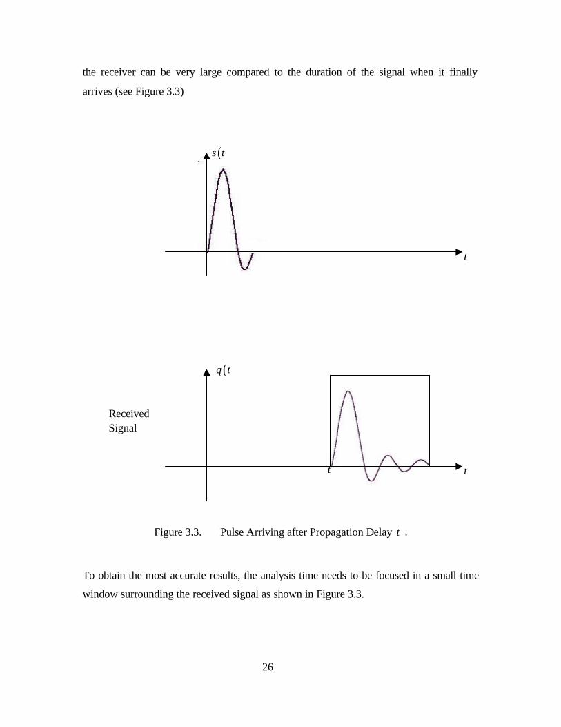
The time intervals encountered in ocean acoustics can be large. In particular the

time due to propagation delay from source to receiver driving which no sound is heard at

26

the receiver can be very large compared to the duration of the signal when it finally

arrives (see Figure 3.3)

Figure 3.3. Pulse Arriving after Propagation Delay τ .

To obtain the most accurate results, the analysis time needs to be focused in a small time

window surrounding the received signal as shown in Figure 3.3.

( )s t

ource

( )q t

Received Signal

t

tτ

27

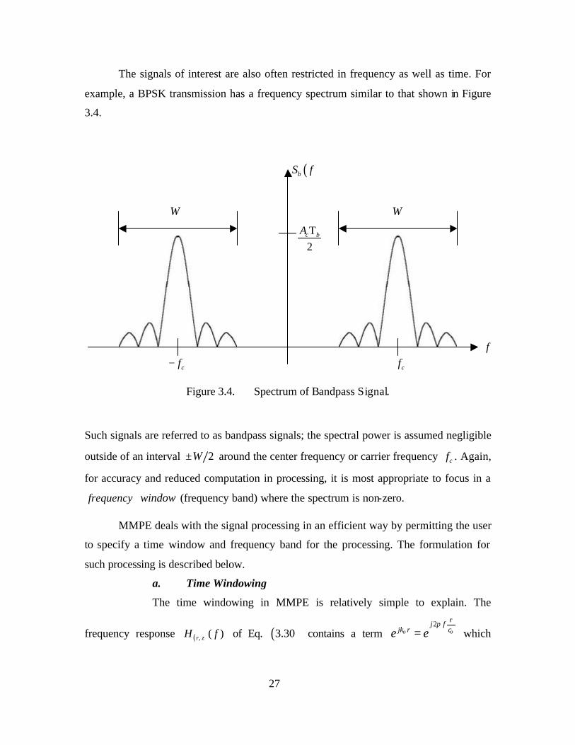
The signals of interest are also often restricted in frequency as well as time. For

example, a BPSK transmission has a frequency spectrum similar to that shown in Figure

3.4.

W W

2c bA Τ

Figure 3.4. Spectrum of Bandpass Signal.

Such signals are referred to as bandpass signals; the spectral power is assumed negligible

outside of an interval 2W± around the center frequency or carrier frequency cf . Again,

for accuracy and reduced computation in processing, it is most appropriate to focus in a

frequency window (frequency band) where the spectrum is non-zero.

MMPE deals with the signal processing in an efficient way by permitting the user

to specify a time window and frequency band for the processing. The formulation for

such processing is described below.

a. Time Windowing

The time windowing in MMPE is relatively simple to explain. The

frequency response ( ) )(, fH zr of Eq. ( )3.30 contains a term 2 rj f

jk r ce eο οπ

= which

cf−

( )bS f

cff

28

corresponds to the gross propagation delay r cοτ = from source to receiver in the ocean.

MMPE drops this term, so that the modified frequency response is given by

( )( , )' 1

( ) , ,r zH f r z fr

= Ψ ( )3.31

The time domain signals resulting from this modified frequency response correspond to a

reduced time scale 't defined as

' rt t t

cο

τ= − = − ( )3.32

and referred to as reduced time . MMPE uses this reduced time for its output results.

Absolute time (relative to the source) can be obtained by adding back in the gross

propagation delay r c οτ = .

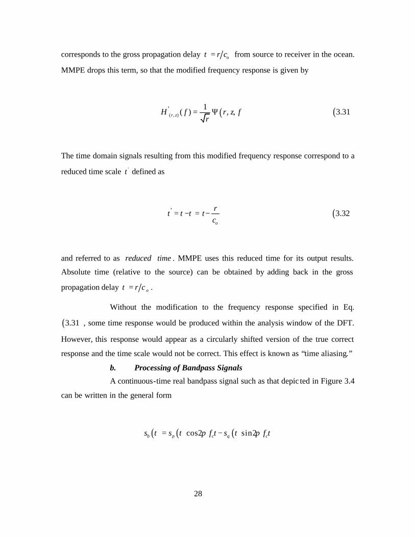
Without the modification to the frequency response specified in Eq.

( )3.31 , some time response would be produced within the analysis window of the DFT.

However, this response would appear as a circularly shifted version of the true correct

response and the time scale would not be correct. This effect is known as “time aliasing.”

b. Processing of Bandpass Signals

A continuous-time real bandpass signal such as that depic ted in Figure 3.4

can be written in the general form

( ) ( ) ( )cos2 sin2b p c q cs t s t f t s t f tπ π= −

29

Here ( )ps t and ( )qs t are known as the “in-phase” and “quadrature” modulation

components. The bandpass signal can be equivalently expressed as

( ) ( ) 2Re cj f tbs t s t e π =

% ( )3.33

where

( ) ( ) ( )p qs t s t js t= +%

is known as the complex envelope . The complex envelope is a complex-valued low-pass

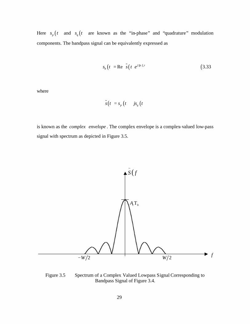
signal with spectrum as depicted in Figure 3.5.

Figure 3.5 Spectrum of a Complex Valued Lowpass Signal Corresponding to Bandpass Signal of Figure 3.4.

f

c bA Τ

2W− 2W

( )fS~

30

The complex envelope may be obtained from the original bandpass signal by discarding

the negative-frequency part of the spectrum, moving the positive-frequency part of the

spectrum from a center point of cf f= to 0f = (“baseband”) and scaling by a factor of

2.

The advantage of using complex envelope representation for the bandpass

signal is that the processing can be focused in the bandpass region by processing the

complex envelope at baseband. Let us denote the sampled version of the complex

envelope as

[ ] ( ) ( ) ( )p qs n s nT s nT js nT= = +%

(The notation [ ]s n was previously used to denote a sampled real band- limited baseband

signal; the only difference now is that [ ]s n is complex.) The complex baseband signal

can be represented as in Eq. ( )3.10 where [ ]S k are the frequency components at

baseband defined by Eq. ( )3.11 . However a frequency in the DFT of 2 k Lπ represents

an actual frequency in the ocean of 2 ck L fπ + . Hence the ocean frequency response

( )1x

H fr must be computed by MMPE at this higher frequency (2 ck L fπ + ). The time-

sampled complex envelope of the received signal is then given by

[ ] [ ]1

21

0

1 2 knL jL

cxk

kq n H f S k e

L L

ππ−

=

= +

∑ r ( )3.34

(Compare this to Eq. ( )3.12 ). The sampled real bandpass signal at the receiver is thus

given by

31

[ ] [ ] 22Re cj f n Tbq n q n e π = ( )3.35

3. Input Parameters for the MMPE Model

The input data for the MMPE model fall into three main categories: the main

input file, the source data, and the environmental data. Each of these is described below.

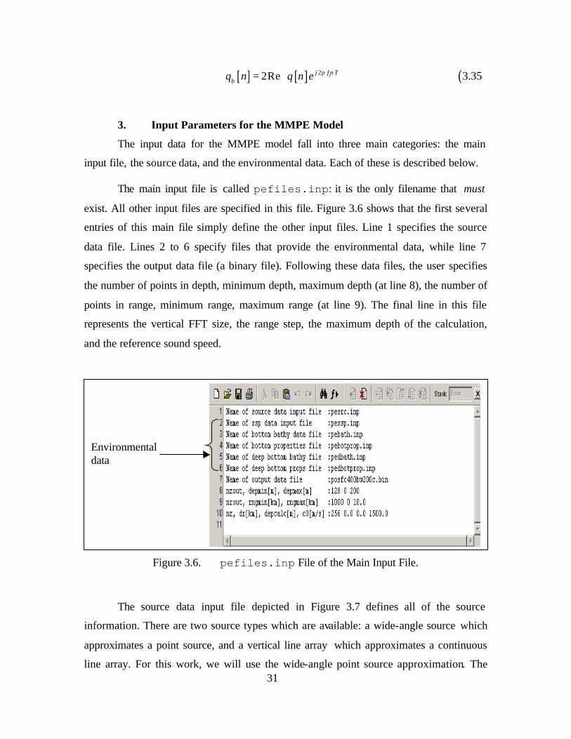
The main input file is called pefiles.inp: it is the only filename that must

exist. All other input files are specified in this file. Figure 3.6 shows that the first several

entries of this main file simply define the other input files. Line 1 specifies the source

data file. Lines 2 to 6 specify files that provide the environmental data, while line 7

specifies the output data file (a binary file). Following these data files, the user specifies

the number of points in depth, minimum depth, maximum depth (at line 8), the number of

points in range, minimum range, maximum range (at line 9). The final line in this file

represents the vertical FFT size, the range step, the maximum depth of the calculation,

and the reference sound speed.

Figure 3.6. pefiles.inp File of the Main Input File.

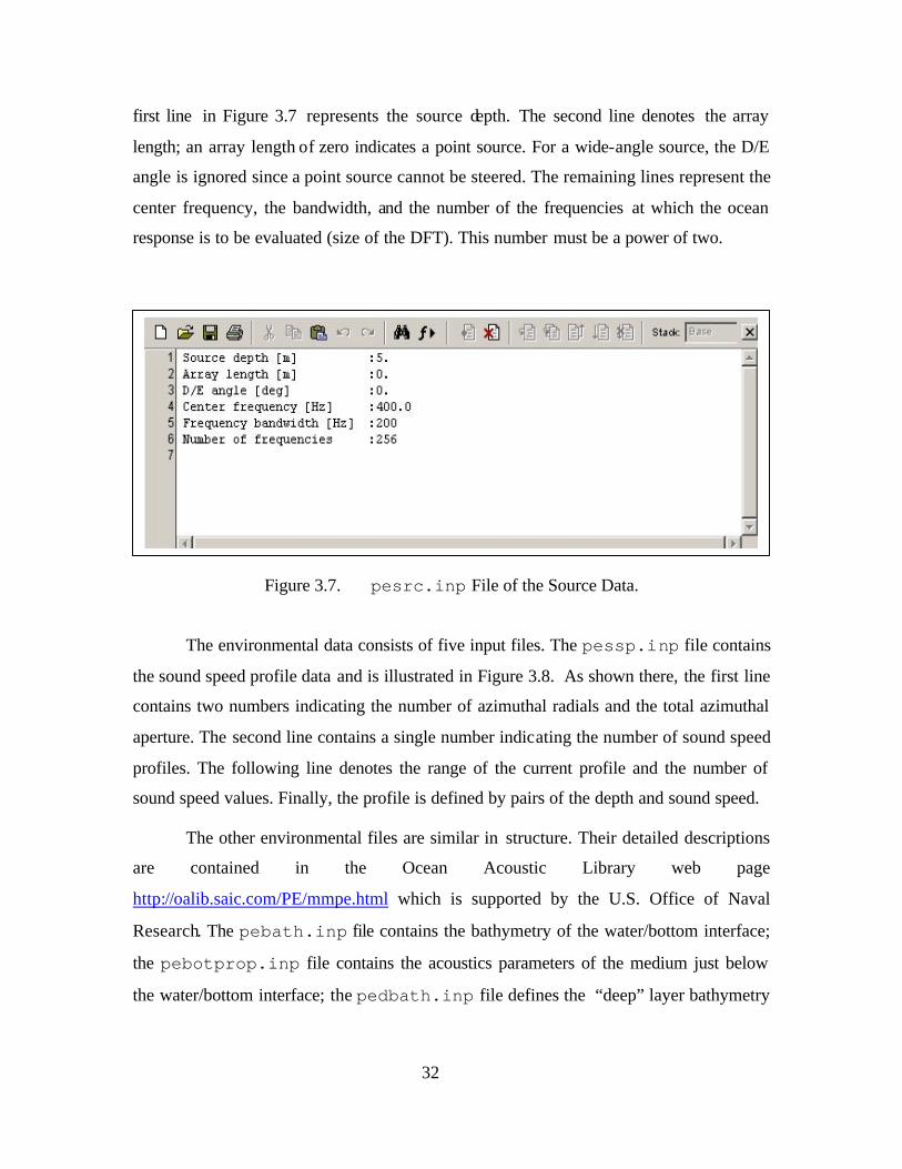
The source data input file depicted in Figure 3.7 defines all of the source

information. There are two source types which are available: a wide-angle source which

approximates a point source, and a vertical line array which approximates a continuous

line array. For this work, we will use the wide-angle point source approximation. The

Environmental data

I* m c* */► @i Stack: Base

Nate of source data input file 2 Nate of ssp data input file 3 Name of bottoi bathy data file

«e of bottoi properties file 5 Name of deep bottoi bathy file

Naie of deep bottoi props file Naie of output data file

8 nzout, depiin[i], depiax[i] nrout, rngiin[lii], rnpax[ki]

0 nz, dr[ki], depcalc[i], cO[i/s]

:pesrc.inp :pessp.inp :pebath.inp :pebotprop.inp ipedbath.inp

:pedbotprop.inp :posfc400bw200c.bin

:128 0 200 :1000 0 10.0 :256 0.0 0.0 1500.0

i±r

32

first line in Figure 3.7 represents the source depth. The second line denotes the array

length; an array length of zero indicates a point source. For a wide-angle source, the D/E

angle is ignored since a point source cannot be steered. The remaining lines represent the

center frequency, the bandwidth, and the number of the frequencies at which the ocean

response is to be evaluated (size of the DFT). This number must be a power of two.

Figure 3.7. pesrc.inp File of the Source Data.

The environmental data consists of five input files. The pessp.inp file contains

the sound speed profile data and is illustrated in Figure 3.8. As shown there, the first line

contains two numbers indicating the number of azimuthal radials and the total azimuthal

aperture. The second line contains a single number indicating the number of sound speed

profiles. The following line denotes the range of the current profile and the number of

sound speed values. Finally, the profile is defined by pairs of the depth and sound speed.

The other environmental files are similar in structure. Their detailed descriptions

are contained in the Ocean Acoustic Library web page

http://oalib.saic.com/PE/mmpe.html which is supported by the U.S. Office of Naval

Research. The pebath.inp file contains the bathymetry of the water/bottom interface;

the pebotprop.inp file contains the acoustics parameters of the medium just below

the water/bottom interface; the pedbath.inp file defines the “deep” layer bathymetry

DtfHi ■■ ü e -o ^ M /► gi Stack: Base xJ Source depth [m] Array length [in] D/E angle [deg] Center frequency [Hz] Frequency bandwidth [Hz] Number of frequencies

5. 0. 0. 400.0 200 256

l>

33

beneath the water/sediment interface; and finally, the pedbotprop.inp file contains

the acoustic properties of the deep layer.

Figure 3.8. pessp.inp File of the Environmental Data.

The last file, the output data file is a binary file produced by MMPE. It is read by the

postprocessing program to produce final results

C. OCEAN ENVIRONMENTAL CHARACTERIZATION

For our simulation studies of underwater communication, we focused on shallow

water environments. Three different ocean environments which have three different

sound speed profiles (SSP) were simulated to test the performance of underwater

communication using a BPSK signal. The complete set of MMPE input files for all three

cases are given in Appendix A.

1. Case 1: Positive SSP Gradient

For this case, the source is located at a range of 0 m and at a depth of 5 m. The

sound speed is range- independent with a positive, linear gradient SSP of 1497 m/s at the

surface and 1499 m/s at a depth of 100m. The density of water is assumed to be 1.0

g/cm3. The bottom is chosen to be a ‘bumpy’ bottom with the following depths: 102m at

0 km; 101 m at 2.5 km; 99m at 5 km; 102 m at 7.5 km; and 99 m at 10 km. Its

compressional sound speed is 1700 m/s, the sound speed gradient 1 1−s , density 1.5

g/cm3, and compressional attenuation 0.1 dB/km/Hz. Figure 3.9 shows the positive

sound speed profile versus depth and the corresponding sound transmission loss plot

D^Bi #* /► a e i t mm Stack: f& J<|

1 2 3 4 5 6 7 8

1 0. 1 0. 4

0.0 1490.0 100.0 1500.0 150.0 1510.0 250.0 1520.0

-1

<l M

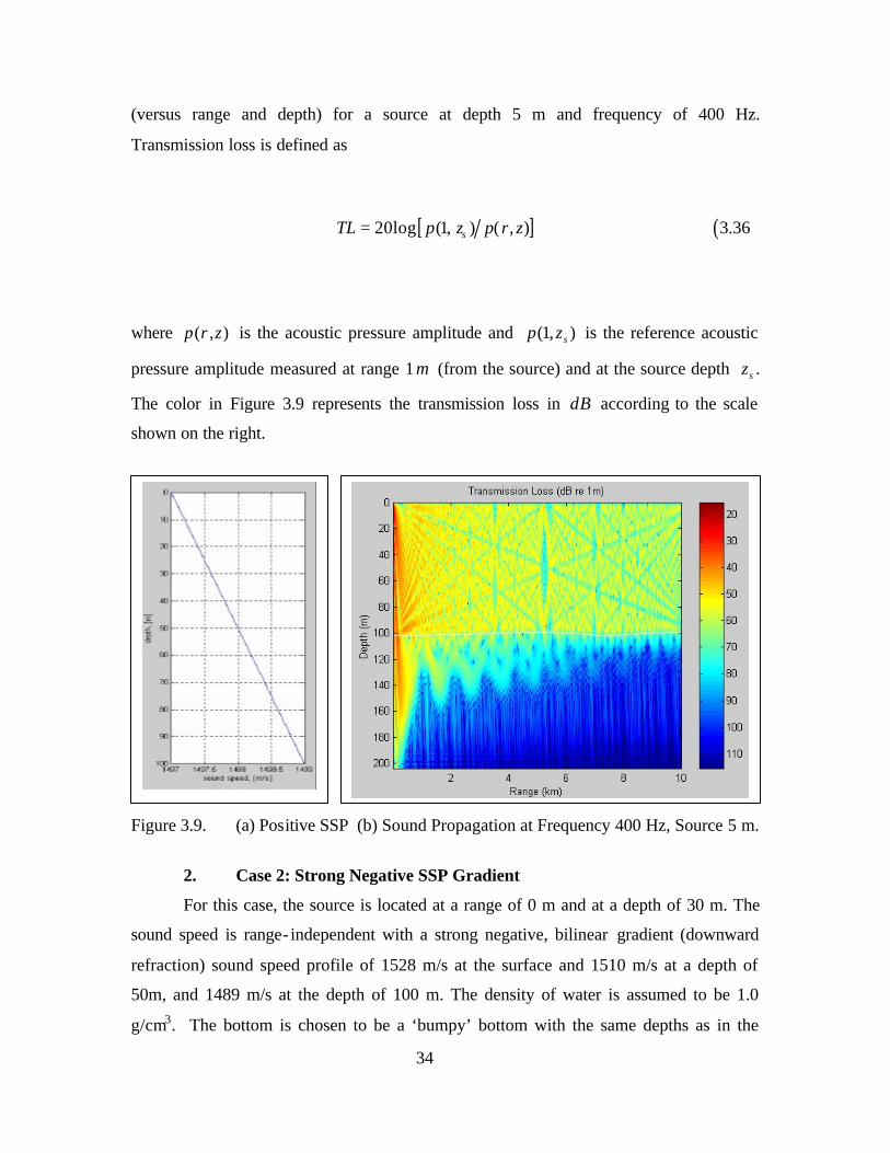
34

(versus range and depth) for a source at depth 5 m and frequency of 400 Hz.

Transmission loss is defined as

[ ]20log (1, ) ( , )sTL p z p r z= ( )3.36

where ( , )p r z is the acoustic pressure amplitude and (1, )sp z is the reference acoustic

pressure amplitude measured at range 1m (from the source) and at the source depth sz .

The color in Figure 3.9 represents the transmission loss in dB according to the scale

shown on the right.

Figure 3.9. (a) Positive SSP (b) Sound Propagation at Frequency 400 Hz, Source 5 m.

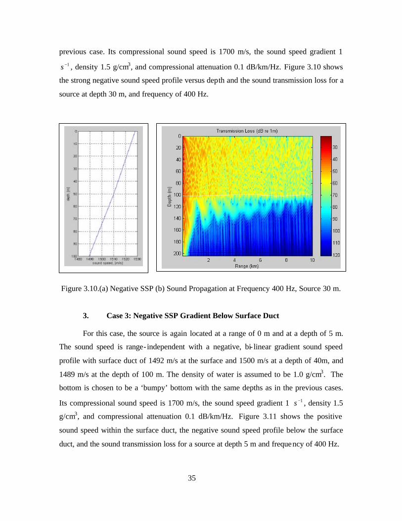
2. Case 2: Strong Negative SSP Gradient

For this case, the source is located at a range of 0 m and at a depth of 30 m. The

sound speed is range- independent with a strong negative, bilinear gradient (downward

refraction) sound speed profile of 1528 m/s at the surface and 1510 m/s at a depth of

50m, and 1489 m/s at the depth of 100 m. The density of water is assumed to be 1.0

g/cm3. The bottom is chosen to be a ‘bumpy’ bottom with the same depths as in the

1* to

f

..A. \ 1

T497 1407t 1498 14305 1409 iduiid ipaaa \m>n

Transmission Loss (dB re 1m)

35

previous case. Its compressional sound speed is 1700 m/s, the sound speed gradient 1 1−s , density 1.5 g/cm3, and compressional attenuation 0.1 dB/km/Hz. Figure 3.10 shows

the strong negative sound speed profile versus depth and the sound transmission loss for a

source at depth 30 m, and frequency of 400 Hz.

Figure 3.10.(a) Negative SSP (b) Sound Propagation at Frequency 400 Hz, Source 30 m.

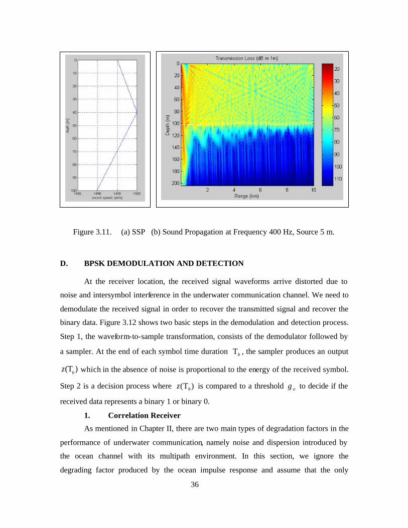
3. Case 3: Negative SSP Gradient Below Surface Duct

For this case, the source is again located at a range of 0 m and at a depth of 5 m.

The sound speed is range- independent with a negative, bi- linear gradient sound speed

profile with surface duct of 1492 m/s at the surface and 1500 m/s at a depth of 40m, and

1489 m/s at the depth of 100 m. The density of water is assumed to be 1.0 g/cm3. The

bottom is chosen to be a ‘bumpy’ bottom with the same depths as in the previous cases.

Its compressional sound speed is 1700 m/s, the sound speed gradient 1 1−s , density 1.5

g/cm3, and compressional attenuation 0.1 dB/km/Hz. Figure 3.11 shows the positive

sound speed within the surface duct, the negative sound speed profile below the surface

duct, and the sound transmission loss for a source at depth 5 m and frequency of 400 Hz.

6

i"

IDJ

«.

..;../..

; /

• /

_j

r ; ; 1 l«0 Iff» 1530 131C «TOT

&DUI4 ipwd. |T>*!|

36

Figure 3.11. (a) SSP (b) Sound Propagation at Frequency 400 Hz, Source 5 m.

D. BPSK DEMODULATION AND DETECTION

At the receiver location, the received signal waveforms arrive distorted due to

noise and intersymbol interference in the underwater communication channel. We need to

demodulate the received signal in order to recover the transmitted signal and recover the

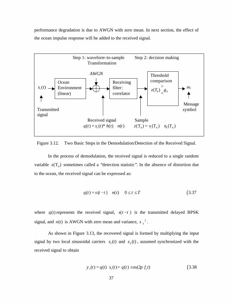
binary data. Figure 3.12 shows two basic steps in the demodulation and detection process.

Step 1, the waveform-to-sample transformation, consists of the demodulator followed by

a sampler. At the end of each symbol time duration bΤ , the sampler produces an output

( )bz Τ which in the absence of noise is proportional to the energy of the received symbol.

Step 2 is a decision process where ( )bz Τ is compared to a threshold ογ to decide if the

received data represents a binary 1 or binary 0.

1. Correlation Receiver

As mentioned in Chapter II, there are two main types of degradation factors in the

performance of underwater communication, namely noise and dispersion introduced by

the ocean channel with its multipath environment. In this section, we ignore the

degrading factor produced by the ocean impulse response and assume that the only

37

performance degradation is due to AWGN with zero mean. In next section, the effect of

the ocean impulse response will be added to the received signal.

Figure 3.12. Two Basic Steps in the Demodulation/Detection of the Received Signal.

In the process of demodulation, the received signal is reduced to a single random

variable ( )bz Τ sometimes called a “detection statistic”. In the absence of distortion due

to the ocean, the received signal can be expressed as:

( ) ( ) ( )q t s t n tτ= − + Tt ≤≤0 ( )3.37

where ( )q t represents the received signal, ( )s t τ− is the transmitted delayed BPSK

signal, and )(tn is AWGN with zero mean and variance, 2οσ .

As shown in Figure 3.13, the recovered signal is formed by multiplying the input

signal by two local sinusoidal carriers )(1 ts and )(2 ts , assumed synchronized with the

received signal to obtain

1 1( ) ( ) ( ) ( ) cos(2 )cy t q t s t q t f tπ= ⋅ = ⋅ ( )3.38

Step 1: waveform-to-sample Step 2: decision making Transformation

AWGN

)(tsi im∧

Message Transmitted symbol signal

Received signal Sample ( ) ( ) ( ) ( )iq t s t h t n t= ∗ + 0( ) ( ) ( )b i b bz v nΤ = Τ + Τ

Receiving filter: correlator

Threshold comparison

0( )bz T γ><

Ocean Environment (linear)

38

and

2 2( ) ( ) ( ) ( ) cos(2 )cy t q t s t q t f tπ= ⋅ = − ⋅ ( )3.39

Figure 3.13. Correlator Receiver.

The recovered signals ( )1y t and ( )2y t are integrated over the bit interval to

obtain

( ) ( ) ( ) ( )i b i iz y t dt q t s t dtΤ = =∫ ∫ 2,1=i ( )3.40

and the outputs of the integrations are subtracted to form the detection statistic

1 2( ) ( ) ( )b b bz z zΤ = Τ − Τ ( )3.41

Local sinusoidal carrier )2cos()(1 tfts cπ=

1( )bz Τ stageDecision

( )( ) ( )

b

i b b

zv n

Τ =Τ + Τ

( )q t im∧

Output (logical 1 ( )2 bz Τ or logical 0)

)2cos()(2 tfts cπ−=

0( )bz γ>

Τ<

∫

∫

∑

39

In the decision stage, ( )bz Τ is compared to an optimum threshold as follows

( )bz T><

1 2

2v v

ογ+

= ( )3.42

where 1v is the signal component of ( )bz Τ when )(1 ts is transmitted, and 2v is the signal

component of ( )bz Τ when )(2 ts is transmitted. The threshold level 0γ defined by

( )1 2 2v vογ = + is the optimum threshold for minimizing the probability of bit error [Ref

1]. For equal energy, equally likely antipodal signals, where )()( 21 tsts −= and 1 2v v= − ,

the decision rule becomes

0( ) 0bz γ>

Τ =<

( )3.43a

Assuming that )(1 ts corresponds to binary 1 and )(2 ts is binary 0, the decision

rule thus reduces to

decide binary 1 if 1 2( ) ( )b bz zΤ > Τ ( )3.43b

decide binary 0 otherwise

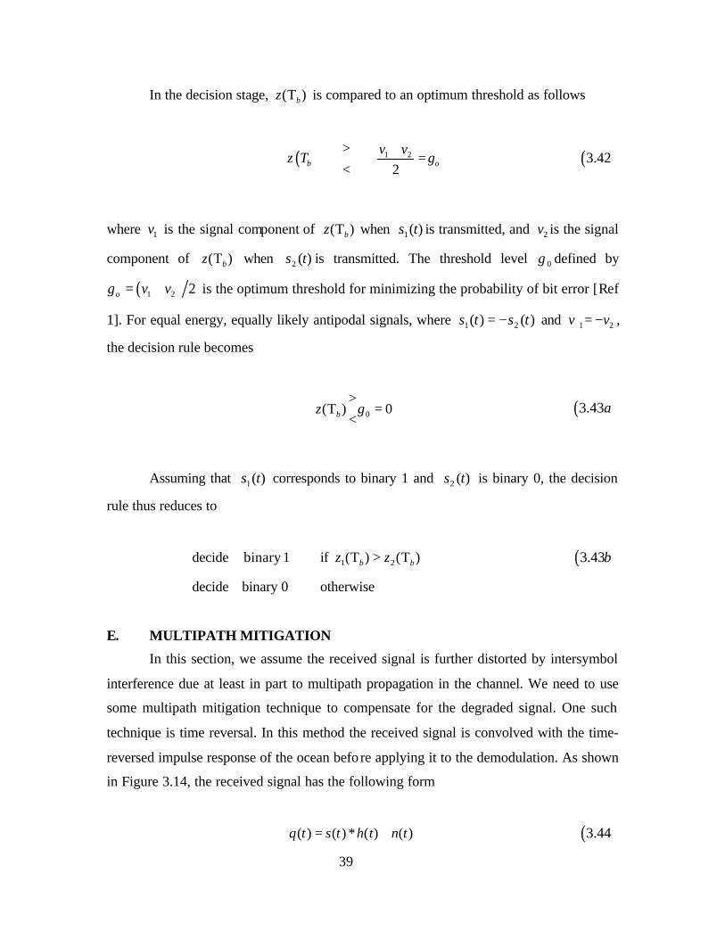
E. MULTIPATH MITIGATION

In this section, we assume the received signal is further distorted by intersymbol

interference due at least in part to multipath propagation in the channel. We need to use

some multipath mitigation technique to compensate for the degraded signal. One such

technique is time reversal. In this method the received signal is convolved with the time-

reversed impulse response of the ocean befo re applying it to the demodulation. As shown

in Figure 3.14, the received signal has the following form

( ) ( ) ( ) ( )q t s t h t n t= ∗ + ( )3.44

40

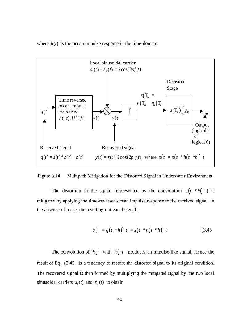
where )(th is the ocean impulse response in the time-domain.

Figure 3.14 Multipath Mitigation for the Distorted Signal in Underwater Environment.

The distortion in the signal (represented by the convolution ( ) ( )s t h t∗ ) is

mitigated by applying the time-reversed ocean impulse response to the received signal. In

the absence of noise, the resulting mitigated signal is

( ) ( ) ( ) ( ) ( ) ( )s t q t h t s t h t h t∧

= ∗ − = ∗ ∗ − ( )3.45

The convolution of ( )h t with ( )h t− produces an impulse-like signal. Hence the

result of Eq. ( )3.45 is a tendency to restore the distorted signal to its original condition.

The recovered signal is then formed by multiplying the mitigated signal by the two local

sinusoidal carriers )(1 ts and )(2 ts to obtain

Local sinusoidal carrier )2cos(2)()( 21 tftsts cπ=−

Decision

Stage

( )( ) ( )

b

i b b

z

v nο

Τ =

Τ + Τ

( )q t im

∧

Output (logical 1 or logical 0)

Received signal Recovered signal

( ) ( ) ( ) ( )q t s t h t n t= ∗ + ( ) ( ) 2cos(2 )cy t s t f tπ∧

= ⋅ , where ( ) ( ) ( ) ( )s t s t h t h t∧

= ∗ ∗ −

0( )bz γ>

Τ<

Time reversed ocean impulse response:

)(),( fHth ∗−

( )y t( )s t$

∫

41

( ) )2cos(2)()()()()( 21 tftststststy cπ⋅=−⋅=∧∧

( )3.46

The recovered signals )(ty are integrated over the bit time duration to form the

detection statistic. This is compared to a threshold as before to produce the recovered

binary data.

42

THIS PAGE INTENTIONALLY LEFT BLANK

43

IV. SIMULATION RESULTS

A. EVALUATION OF BIT ERROR PROBABILITY FOR BPSK SIGNAL

In this section, the parameters (bandwidth, sampling frequency, bit rate, samples

per bit, interpolation factor and up-sampling frequency) for the BPSK signal and a Finite

Impulse Response (FIR) filter are defined, and the effect of the AWGN on the bit error

performance is evaluated.

1. Evaluation for BPSK Parameters

An important theorem of communication is based on the assumption of a strictly

bandlimited channel, i.e. one in which no signal power whatever is allowed outside the

band of interest. For our work, we need to define the bandwidth for the BPSK signal

transmission. The single-sided power spectral density for the BPSK signal (also known as

the analytic signal) is given by

( )( )

22 sin

( )4

c bc bBPSK

c b

f fAP f

f fπ

π+ − ΤΤ

= − Τ

( )1.4

This follows from Eq. ( )3.8 by dropping the terms for negative frequencies. This

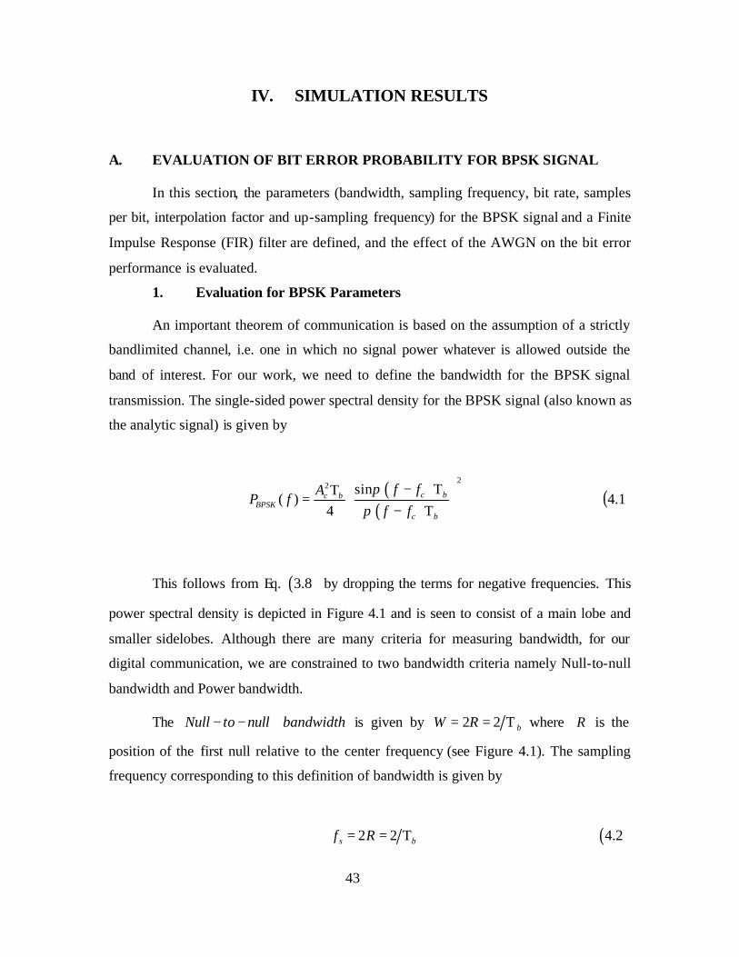
power spectral density is depicted in Figure 4.1 and is seen to consist of a main lobe and

smaller sidelobes. Although there are many criteria for measuring bandwidth, for our

digital communication, we are constrained to two bandwidth criteria namely Null-to-null

bandwidth and Power bandwidth.

The Null to null− − bandwidth is given by 2 2 bW R= = Τ where R is the

position of the first null relative to the center frequency (see Figure 4.1). The sampling

frequency corresponding to this definition of bandwidth is given by

2 2s bf R= = Τ ( )4.2

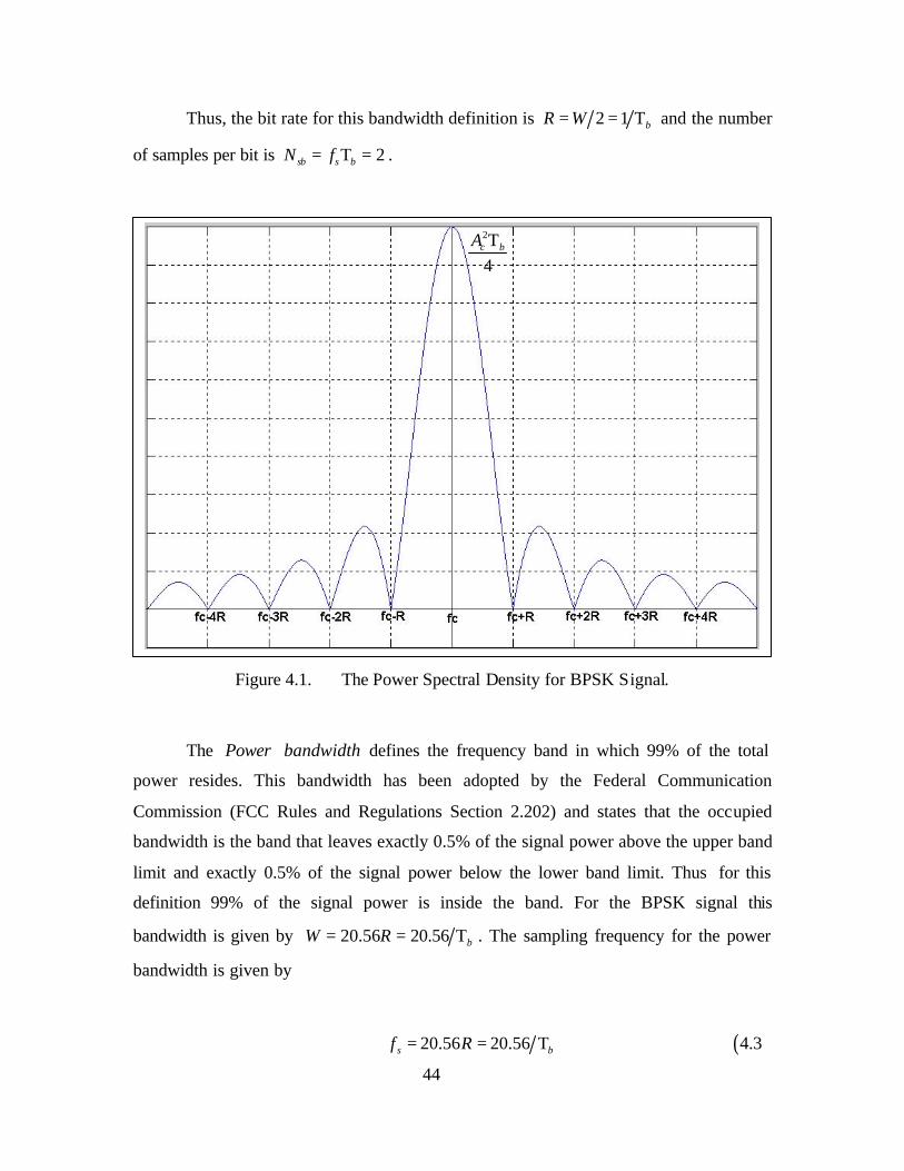
44

Thus, the bit rate for this bandwidth definition is 2 1 bR W= = Τ and the number

of samples per bit is 2sb s bN f= Τ = .

Figure 4.1. The Power Spectral Density for BPSK Signal.

The Power bandwidth defines the frequency band in which 99% of the total

power resides. This bandwidth has been adopted by the Federal Communication

Commission (FCC Rules and Regulations Section 2.202) and states that the occupied

bandwidth is the band that leaves exactly 0.5% of the signal power above the upper band

limit and exactly 0.5% of the signal power below the lower band limit. Thus for this

definition 99% of the signal power is inside the band. For the BPSK signal this

bandwidth is given by 20.56 20.56 bW R= = Τ . The sampling frequency for the power

bandwidth is given by

20.56 20.56s bf R= = Τ ( )4.3

2

4c bA Τ

11111/ \ ! ! ! !

\ 1 1 1 1 <. <. •_ -___J_ ....I.... \ I

\ i i ! !

I III/ till 1 111!!

j j 1 . Z.>_ - -I- H \w f V VVA

fct4R fc^R fq-2R fq-R f: fc+R f<?+2R fc+3R fc+4R I I I I ! ! ! !

III!! ! ! ! !

45

Thus, the bit rate for this bandwidth is 20.56 1 bR W= = Τ and the number of

samples per bit is 20.56sb s bN f= Τ = .

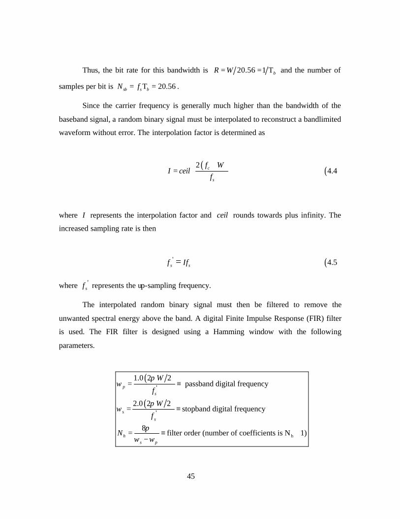
Since the carrier frequency is generally much higher than the bandwidth of the

baseband signal, a random binary signal must be interpolated to reconstruct a bandlimited

waveform without error. The interpolation factor is determined as

( )2 c

s

f WI ceil

f+

=

( )4.4

where I represents the interpolation factor and ceil rounds towards plus infinity. The

increased sampling rate is then

's sf If= ( )4.5

where 'sf represents the up-sampling frequency.

The interpolated random binary signal must then be filtered to remove the

unwanted spectral energy above the band. A digital Finite Impulse Response (FIR) filter

is used. The FIR filter is designed using a Hamming window with the following

parameters.

( )

( )s

h

'

'

1.0 2 2 passband digital frequency

2.0 2 2stopband digital frequency

8filter order (number of coefficients is N 1)

ps

s

hs p

W

f

W

f

N

πω

πω

πω ω

= ≡

= ≡

= ≡ +−

46

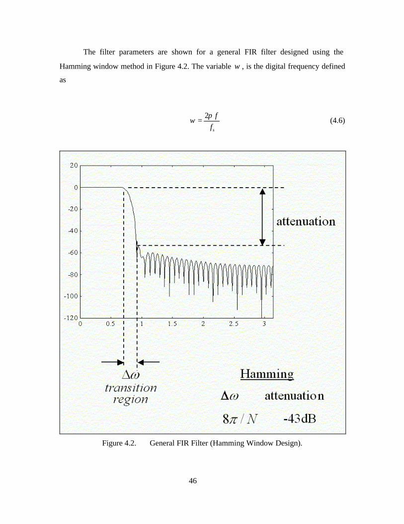
The filter parameters are shown for a general FIR filter designed using the

Hamming window method in Figure 4.2. The variable ω , is the digital frequency defined

as

2

s

ff

πω = (4.6)

Figure 4.2. General FIR Filter (Hamming Window Design).

47

In the following experiments, the frequency response of the BPSK signal for the

Null-to-null bandwidth and Power bandwidth is shown. Figure 4.3 shows the frequency

response for 1000 bits of a BPSK signal which is sampled according to the Null-to-null

bandwidth and has parameters R =100 bits/sec, cf =400 Hz, sf =200 Hz. sbN =2, 6I =

and ' 1200sf = Hz. Figure 4.4 shows the frequency response for 1000 bits of a BPSK

signal which is sampled according to the Power bandwidth criterion with parameters

R =100 bits/sec, cf =4000 Hz, sf =2100 Hz, 6I = , ' 12600sf = Hz and sbN =21

= ( )20.56ceil . The complete procedures to generate the BPSK signal are explained in

Appendix B.

Figure 4.3. Frequency Response for BPSK Signal Sampled by Null- to-null

Bandwidth.

Figure 4.4. Frequency Response for BPSK Signal Sampled by Power Bandwidth.

As shown in Figure 4.3 and Figure 4.4, sampling according to the Power

bandwidth is more reliable than the Null- to-null bandwidth since 99% of the signal power

is within the bandwidth. However, since the most energy is contained within the Null- to-

null bandwidth, it is sufficient to work with the Null-to-null bandwidth for our work. In

Frcquarcy Response <l BPSK Syral al fc= iOO Hi

Frequency Response crt BPSK Signoi a fc- OD Hr

1 BOD |

■■('

< - T" -

I '. I -.1 ; II D Ml «D I i: Frequency (Hü)

48

the next subsection, the bit error performance under AWGN for BPSK signal having

Null-to-null bandwidth is evaluated.

2. Influence of AWGN on Bit Error Probability

For evaluation of the bit error performance under AWGN, the bit error probability

was tested for various values of the average signal power to average noise power ratio

( SNR ). The average signal power was kept constant.

The average signal power to average noise power ratio is defined as SNR = 2b

tοσΕ

∆

where bΕ =2

2bcA Τ

is the average signal power, 2οσ is the white Gaussian noise variance,

and b

sb

tNΤ

∆ = . The SNR is thus given by

SNR =2

22c bA

tοσΤ∆

( )4.7

or in decibels as

SNR (dB)=10log ( SNR )

∆Τ

=t

A bc2

2

2log10

οσ ( )4.8

The theoretical value of the bit error probability ΒΡ from Eq. ( )2.19 is:

( )2

2

22

b c bB

AQ Q SNR Q

N tο οσ

Ε ΤΡ = = = ∆

( )4.9

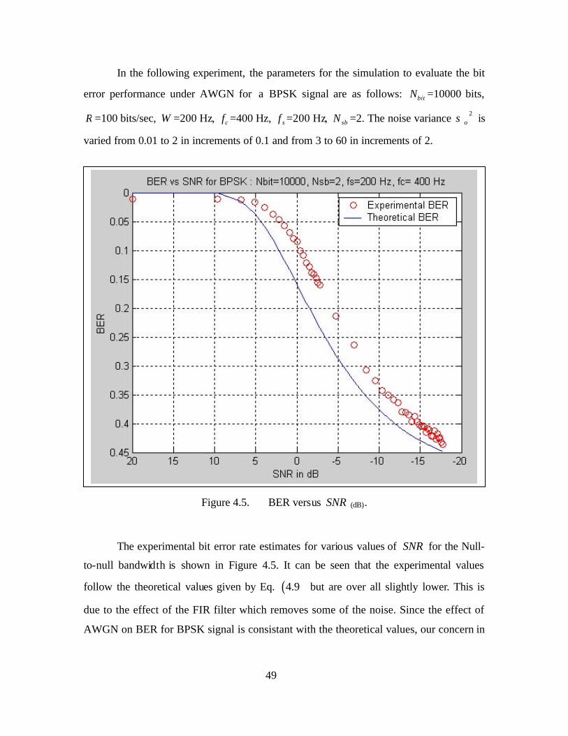
49

In the following experiment, the parameters for the simulation to evaluate the bit

error performance under AWGN for a BPSK signal are as follows: bitN =10000 bits,

R =100 bits/sec, W =200 Hz, cf =400 Hz, sf =200 Hz, sbN =2. The noise variance 2οσ is

varied from 0.01 to 2 in increments of 0.1 and from 3 to 60 in increments of 2.

Figure 4.5. BER versus SNR (dB).

The experimental bit error rate estimates for various values of SNR for the Null-

to-null bandwidth is shown in Figure 4.5. It can be seen that the experimental values

follow the theoretical values given by Eq. ( )4.9 but are over all slightly lower. This is

due to the effect of the FIR filter which removes some of the noise. Since the effect of

AWGN on BER for BPSK signal is consistant with the theoretical values, our concern in

BER YS SNR for BPSK : Nbit=1QGGG. Nsb=2. fs=200 Hz. fc= 400 Hz

5 0-5 SNR in dB

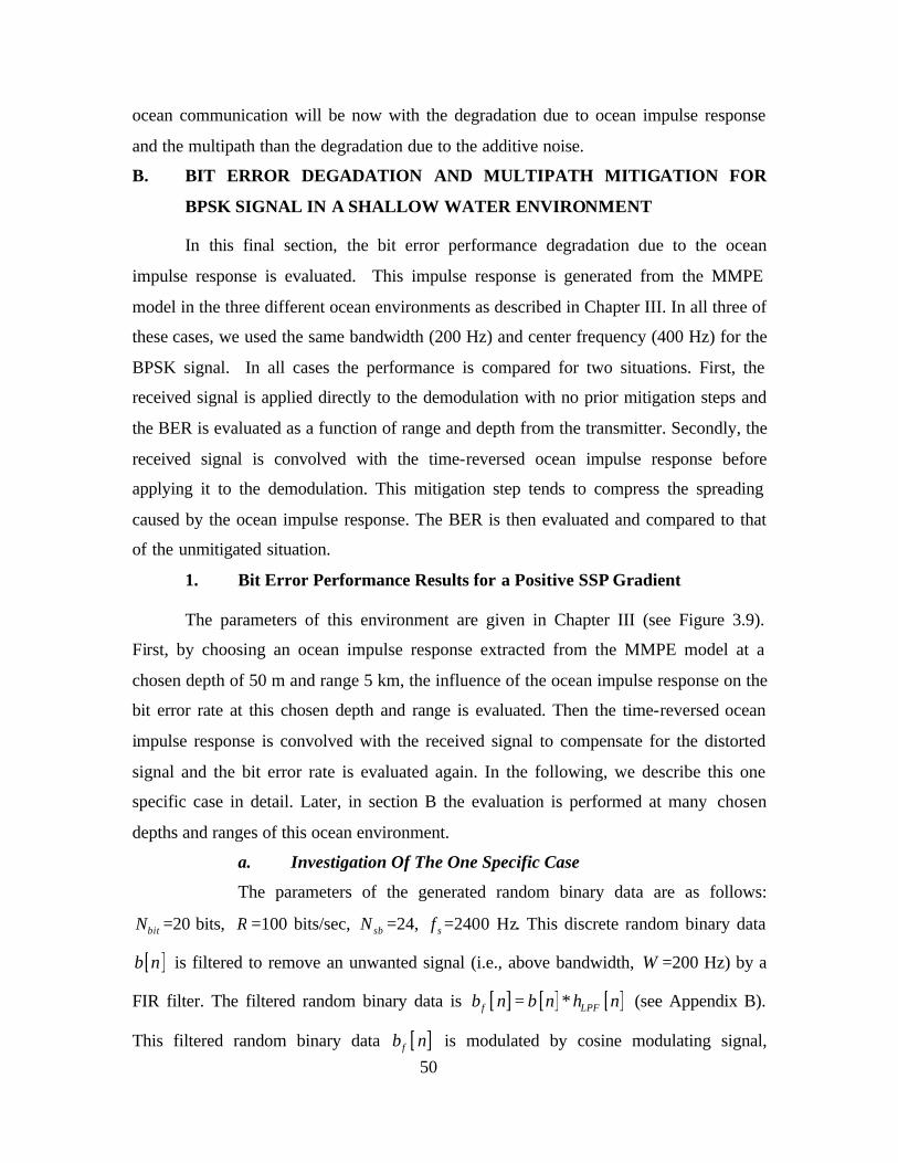
50

ocean communication will be now with the degradation due to ocean impulse response

and the multipath than the degradation due to the additive noise.

B. BIT ERROR DEGADATION AND MULTIPATH MITIGATION FOR

BPSK SIGNAL IN A SHALLOW WATER ENVIRONMENT

In this final section, the bit error performance degradation due to the ocean

impulse response is evaluated. This impulse response is generated from the MMPE

model in the three different ocean environments as described in Chapter III. In all three of

these cases, we used the same bandwidth (200 Hz) and center frequency (400 Hz) for the

BPSK signal. In all cases the performance is compared for two situations. First, the

received signal is applied directly to the demodulation with no prior mitigation steps and

the BER is evaluated as a function of range and depth from the transmitter. Secondly, the

received signal is convolved with the time-reversed ocean impulse response before

applying it to the demodulation. This mitigation step tends to compress the spreading

caused by the ocean impulse response. The BER is then evaluated and compared to that

of the unmitigated situation.

1. Bit Error Performance Results for a Positive SSP Gradient

The parameters of this environment are given in Chapter III (see Figure 3.9).

First, by choosing an ocean impulse response extracted from the MMPE model at a

chosen depth of 50 m and range 5 km, the influence of the ocean impulse response on the

bit error rate at this chosen depth and range is evaluated. Then the time-reversed ocean

impulse response is convolved with the received signal to compensate for the distorted

signal and the bit error rate is evaluated again. In the following, we describe this one

specific case in detail. Later, in section B the evaluation is performed at many chosen

depths and ranges of this ocean environment.

a. Investigation Of The One Specific Case

The parameters of the generated random binary data are as follows:

bitN =20 bits, R =100 bits/sec, sbN =24, sf =2400 Hz. This discrete random binary data

[ ]b n is filtered to remove an unwanted signal (i.e., above bandwidth, W =200 Hz) by a

FIR filter. The filtered random binary data is [ ] [ ] [ ]f LPFb n b n h n= ∗ (see Appendix B).

This filtered random binary data [ ]fb n is modulated by cosine modulating signal,

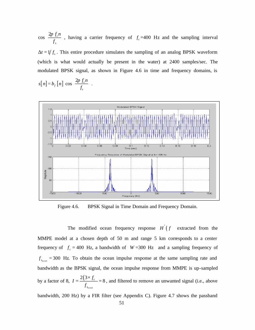
51

2cos c

s

f nf

π

, having a carrier frequency of cf =400 Hz and the sampling interval

1 st f∆ = . This entire procedure simulates the sampling of an analog BPSK waveform

(which is what would actually be present in the water) at 2400 samples/sec. The

modulated BPSK signal, as shown in Figure 4.6 in time and frequency domains, is

[ ] [ ] 2cos c

fs

f ns n b n

fπ

= ⋅

.

Figure 4.6. BPSK Signal in Time Domain and Frequency Domain.

The modified ocean frequency response ( )'H f extracted from the

MMPE model at a chosen depth of 50 m and range 5 km corresponds to a center

frequency of 400cf = Hz, a bandwidth of W =300 Hz and a sampling frequency of

300oceansf = Hz. To obtain the ocean impulse response at the same sampling rate and

bandwidth as the BPSK signal, the ocean impulse response from MMPE is up-sampled

by a factor of 8, ( )2 3

8ocean

c

s

fI

f×

= = , and filtered to remove an unwanted signal (i.e., above

bandwidth, 200 Hz) by a FIR filter (see Appendix C). Figure 4.7 shows the passband

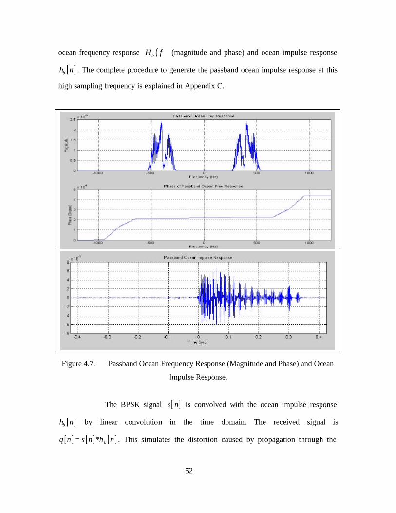
52

ocean frequency response ( )bH f (magnitude and phase) and ocean impulse response

[ ]bh n . The complete procedure to generate the passband ocean impulse response at this

high sampling frequency is explained in Appendix C.

Figure 4.7. Passband Ocean Frequency Response (Magnitude and Phase) and Ocean

Impulse Response.

The BPSK signal [ ]s n is convolved with the ocean impulse response

[ ]bh n by linear convolution in the time domain. The received signal is

[ ] [ ] [ ]bq n s n h n= ∗ . This simulates the distortion caused by propagation through the

0 Time (sot)

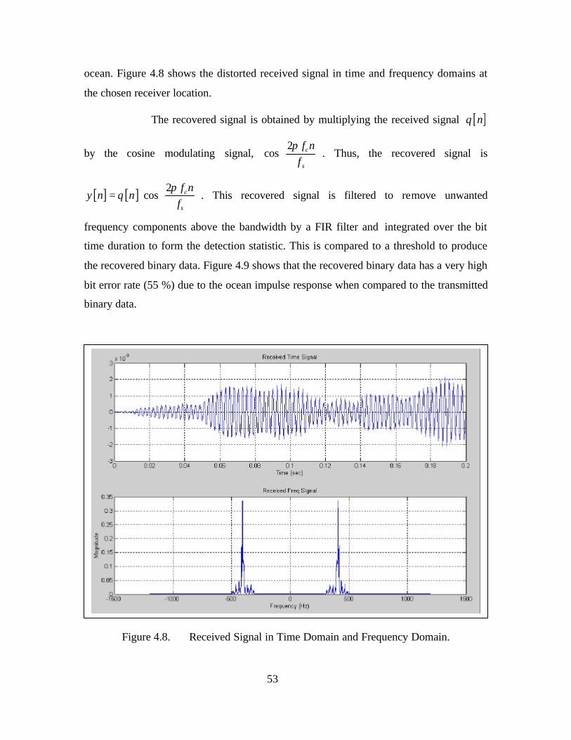
53

ocean. Figure 4.8 shows the distorted received signal in time and frequency domains at

the chosen receiver location.

The recovered signal is obtained by multiplying the received signal [ ]q n

by the cosine modulating signal, 2

cos c

s

f nf

π

. Thus, the recovered signal is

[ ] [ ] 2cos c

s

f ny n q n

fπ

= ⋅

. This recovered signal is filtered to remove unwanted

frequency components above the bandwidth by a FIR filter and integrated over the bit

time duration to form the detection statistic. This is compared to a threshold to produce

the recovered binary data. Figure 4.9 shows that the recovered binary data has a very high

bit error rate (55 %) due to the ocean impulse response when compared to the transmitted

binary data.

Figure 4.8. Received Signal in Time Domain and Frequency Domain.

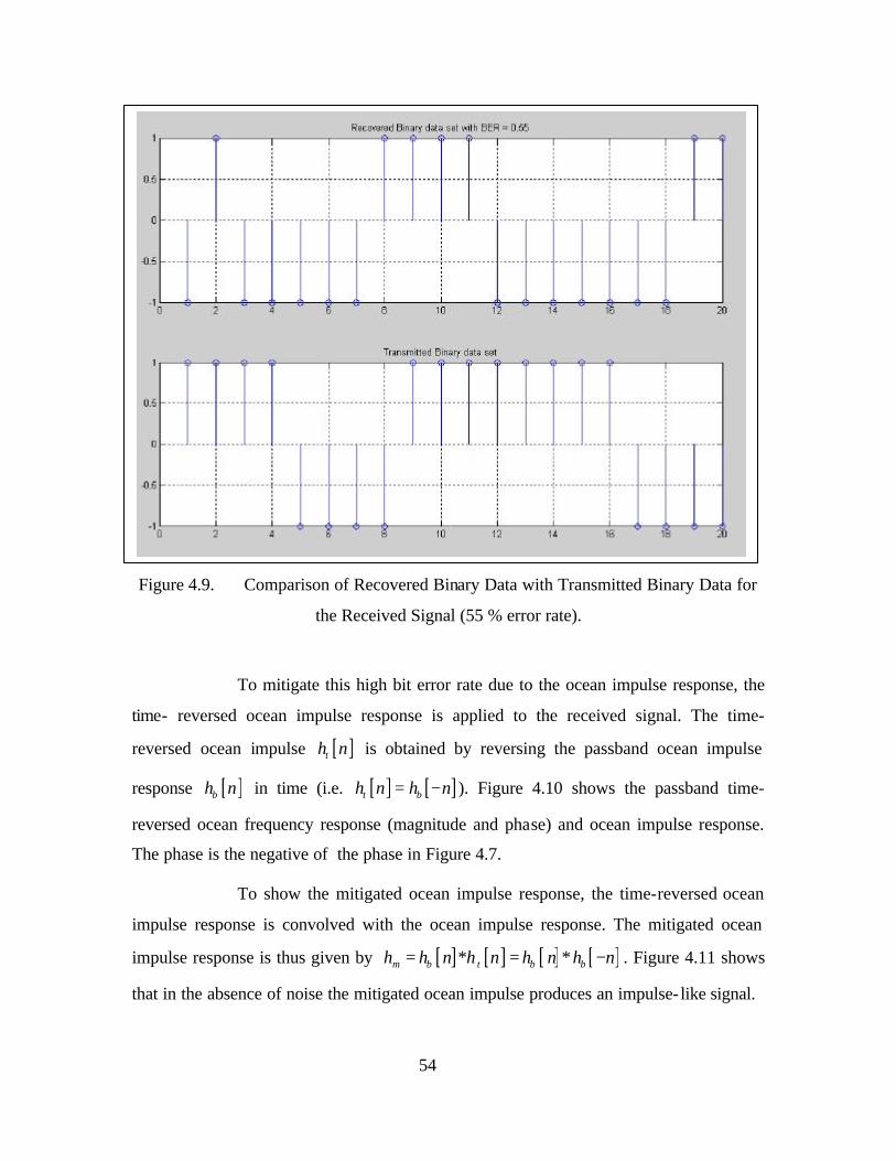
54

Figure 4.9. Comparison of Recovered Binary Data with Transmitted Binary Data for

the Received Signal (55 % error rate).

To mitigate this high bit error rate due to the ocean impulse response, the

time- reversed ocean impulse response is applied to the received signal. The time-

reversed ocean impulse [ ]th n is obtained by reversing the passband ocean impulse

response [ ]bh n in time (i.e. [ ] [ ]t bh n h n= − ). Figure 4.10 shows the passband time-

reversed ocean frequency response (magnitude and phase) and ocean impulse response.

The phase is the negative of the phase in Figure 4.7.

To show the mitigated ocean impulse response, the time-reversed ocean

impulse response is convolved with the ocean impulse response. The mitigated ocean

impulse response is thus given by [ ] [ ] [ ] [ ]m b t b bh h n h n h n h n= ∗ = ∗ − . Figure 4.11 shows

that in the absence of noise the mitigated ocean impulse produces an impulse- like signal.

1 > *. Rscn-sied Binary data set wlh BER = 0.56 1 \ rt 1

0.5

a

•0.5

1

1 T F ' 1 < ' r i 1 i 1 ' i < i

i 1 1 i

J i i i i i • i i , < i i i i i i i 11 i i £

\ ) - 2 " * * 6 10 ii ' ■ n - • % ~ is 33

1

0.6

:

\ > *. > a t *. Transmuted Binary data set i*. j*\ ^*. > *. t * J * t * V \ ■ i "^ K T ^ I r | ! i 1 i ! i i 1 I ■

1 1 f i

i i

1

i i

i

* 1

] ] j i , f fi i i

10 12 u is v & a

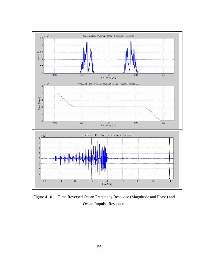
55

Figure 4.10. Time Reversed Ocean Frequency Response (Magnitude and Phase) and

Ocean Impulse Response.

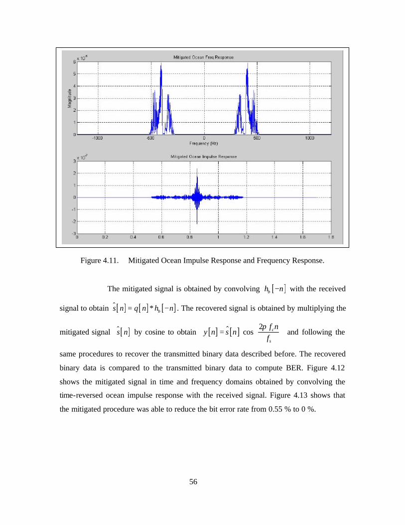
56

Figure 4.11. Mitigated Ocean Impulse Response and Frequency Response.

The mitigated signal is obtained by convolving [ ]bh n− with the received

signal to obtain [ ] [ ] [ ]bs n q n h n= ∗ −$ . The recovered signal is obtained by multiplying the

mitigated signal [ ]s n$ by cosine to obtain [ ] [ ] 2cos c

s

f ny n s n

fπ

= ⋅

$ and following the

same procedures to recover the transmitted binary data described before. The recovered

binary data is compared to the transmitted binary data to compute BER. Figure 4.12

shows the mitigated signal in time and frequency domains obtained by convolving the

time-reversed ocean impulse response with the received signal. Figure 4.13 shows that

the mitigated procedure was able to reduce the bit error rate from 0.55 % to 0 %.

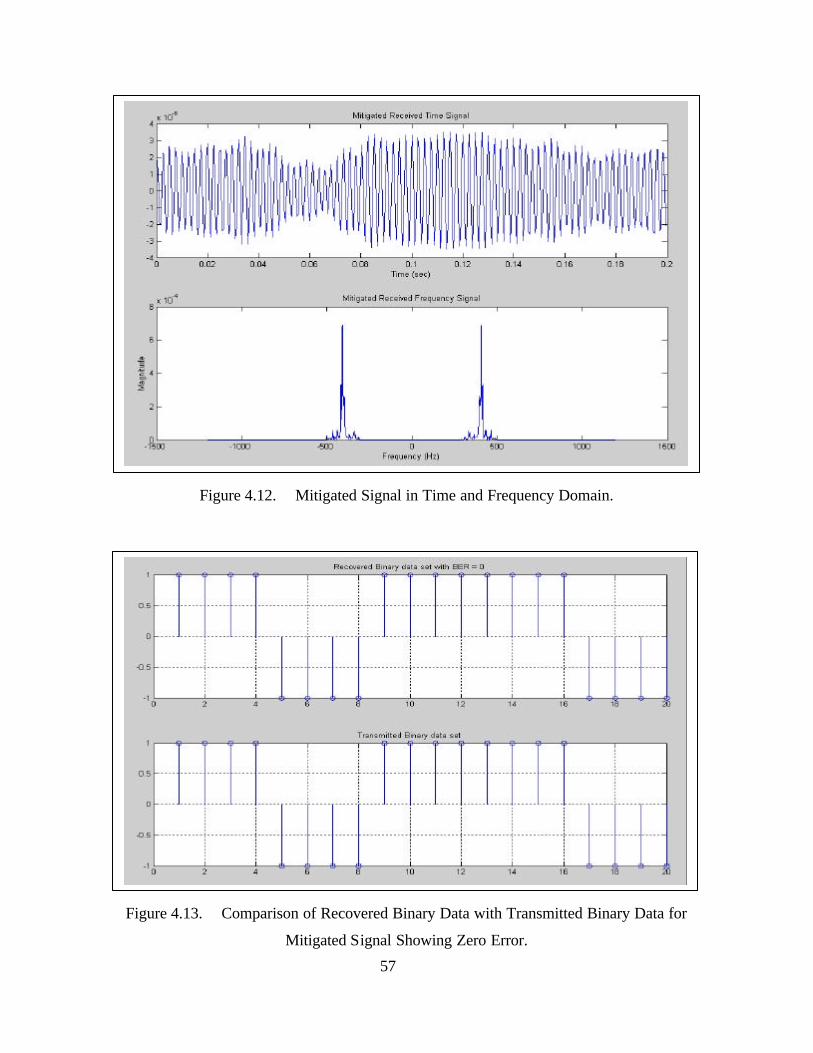
57

Figure 4.12. Mitigated Signal in Time and Frequency Domain.

Figure 4.13. Comparison of Recovered Binary Data with Transmitted Binary Data for

Mitigated Signal Showing Zero Error.

Racovarad Binary dal a gal «ill EER = D

05

•

1 1 T 1 T K s * p ( s <

j

|

i i i

i 1 2 a

> j « 1—! j

i i i i i. i 10 12 14 16

1 1 1

1 1 ~t\

■

rianamitted 9 ■■-1/ data ; -1 1 © c 1 K p ( ! ! —* 1 T 3 C |J * 3 I 1 I ' I

I j j | j f j

! ^ L_ . L I

1 ! ! i i i i ( , ■t 1 t ;.

< 1 1 ' j i i . i i a 1 2 1 A i 3 i J a

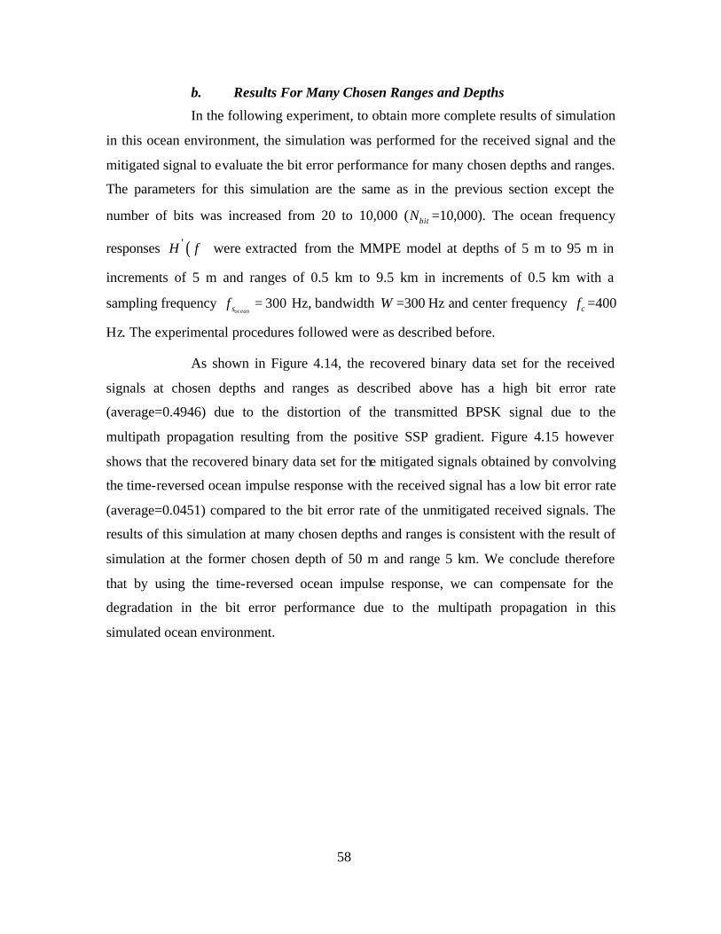
58

b. Results For Many Chosen Ranges and Depths

In the following experiment, to obtain more complete results of simulation

in this ocean environment, the simulation was performed for the received signal and the

mitigated signal to evaluate the bit error performance for many chosen depths and ranges.

The parameters for this simulation are the same as in the previous section except the

number of bits was increased from 20 to 10,000 ( bitN =10,000). The ocean frequency

responses ( )'H f were extracted from the MMPE model at depths of 5 m to 95 m in

increments of 5 m and ranges of 0.5 km to 9.5 km in increments of 0.5 km with a

sampling frequency 300oceansf = Hz, bandwidth W =300 Hz and center frequency cf =400

Hz. The experimental procedures followed were as described before.

As shown in Figure 4.14, the recovered binary data set for the received

signals at chosen depths and ranges as described above has a high bit error rate

(average=0.4946) due to the distortion of the transmitted BPSK signal due to the

multipath propagation resulting from the positive SSP gradient. Figure 4.15 however

shows that the recovered binary data set for the mitigated signals obtained by convolving

the time-reversed ocean impulse response with the received signal has a low bit error rate

(average=0.0451) compared to the bit error rate of the unmitigated received signals. The

results of this simulation at many chosen depths and ranges is consistent with the result of

simulation at the former chosen depth of 50 m and range 5 km. We conclude therefore

that by using the time-reversed ocean impulse response, we can compensate for the

degradation in the bit error performance due to the multipath propagation in this

simulated ocean environment.

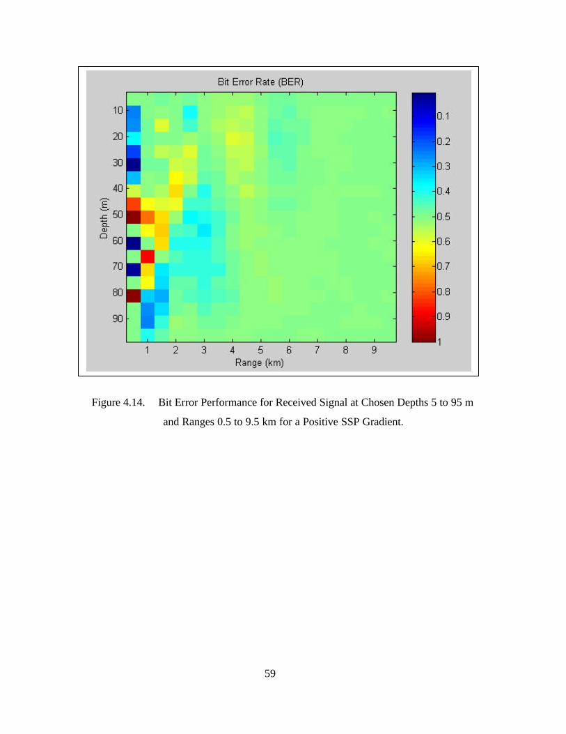
59

Figure 4.14. Bit Error Performance for Received Signal at Chosen Depths 5 to 95 m

and Ranges 0.5 to 9.5 km for a Positive SSP Gradient.

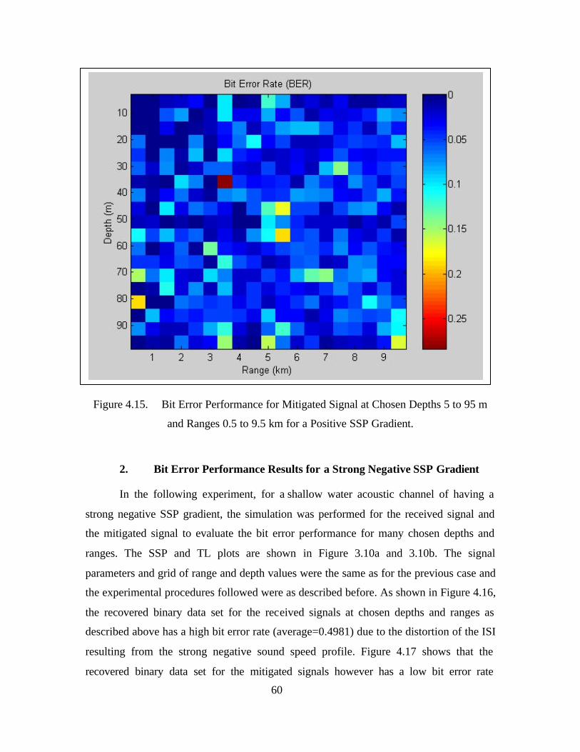
60

Figure 4.15. Bit Error Performance for Mitigated Signal at Chosen Depths 5 to 95 m

and Ranges 0.5 to 9.5 km for a Positive SSP Gradient.

2. Bit Error Performance Results for a Strong Negative SSP Gradient

In the following experiment, for a shallow water acoustic channel of having a

strong negative SSP gradient, the simulation was performed for the received signal and

the mitigated signal to evaluate the bit error performance for many chosen depths and

ranges. The SSP and TL plots are shown in Figure 3.10a and 3.10b. The signal

parameters and grid of range and depth values were the same as for the previous case and

the experimental procedures followed were as described before. As shown in Figure 4.16,

the recovered binary data set for the received signals at chosen depths and ranges as

described above has a high bit error rate (average=0.4981) due to the distortion of the ISI

resulting from the strong negative sound speed profile. Figure 4.17 shows that the

recovered binary data set for the mitigated signals however has a low bit error rate

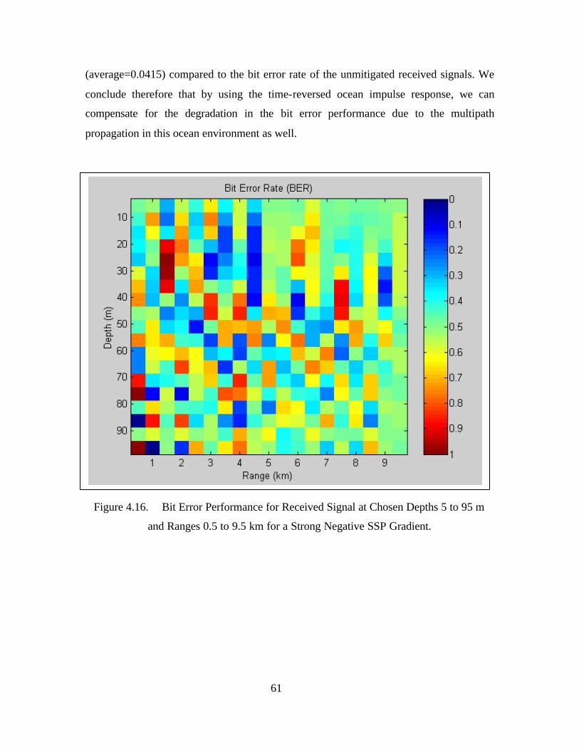
61

(average=0.0415) compared to the bit error rate of the unmitigated received signals. We

conclude therefore that by using the time-reversed ocean impulse response, we can

compensate for the degradation in the bit error performance due to the multipath

propagation in this ocean environment as well.

Figure 4.16. Bit Error Performance for Received Signal at Chosen Depths 5 to 95 m

and Ranges 0.5 to 9.5 km for a Strong Negative SSP Gradient.

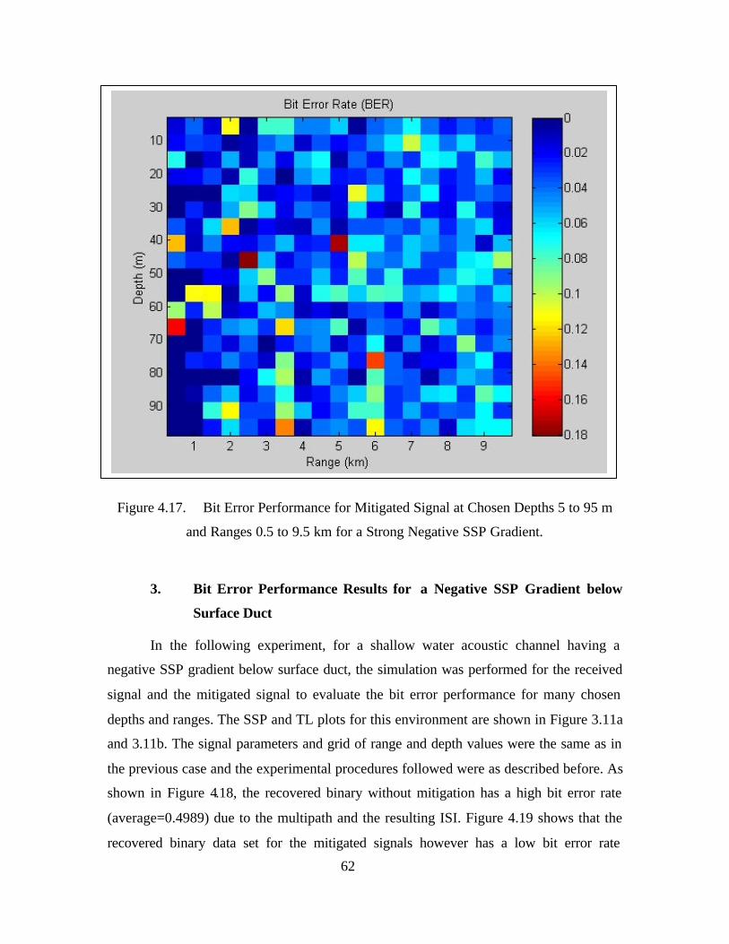
62

Figure 4.17. Bit Error Performance for Mitigated Signal at Chosen Depths 5 to 95 m

and Ranges 0.5 to 9.5 km for a Strong Negative SSP Gradient.

3. Bit Error Performance Results for a Negative SSP Gradient below

Surface Duct

In the following experiment, for a shallow water acoustic channel having a

negative SSP gradient below surface duct, the simulation was performed for the received

signal and the mitigated signal to evaluate the bit error performance for many chosen

depths and ranges. The SSP and TL plots for this environment are shown in Figure 3.11a

and 3.11b. The signal parameters and grid of range and depth values were the same as in

the previous case and the experimental procedures followed were as described before. As

shown in Figure 4.18, the recovered binary without mitigation has a high bit error rate

(average=0.4989) due to the multipath and the resulting ISI. Figure 4.19 shows that the

recovered binary data set for the mitigated signals however has a low bit error rate

4 5 6 Range (km)

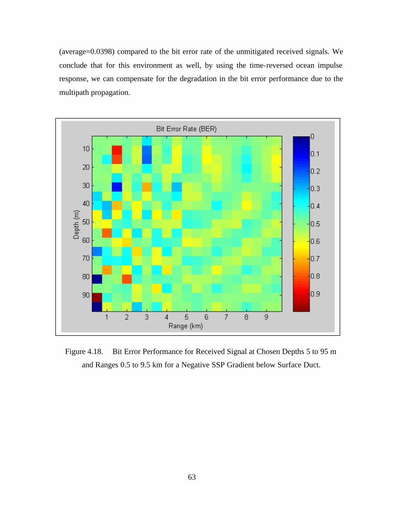
63

(average=0.0398) compared to the bit error rate of the unmitigated received signals. We

conclude that for this environment as well, by using the time-reversed ocean impulse

response, we can compensate for the degradation in the bit error performance due to the

multipath propagation.

Figure 4.18. Bit Error Performance for Received Signal at Chosen Depths 5 to 95 m

and Ranges 0.5 to 9.5 km for a Negative SSP Gradient below Surface Duct.

Bit Error Rate (BER)

I ■

12 3 4 5 6 Range (km)

■0.4

0.5

■06

■0.7

08

0.9

8

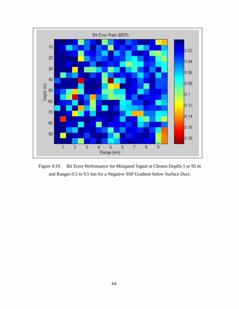
64

Figure 4.19. Bit Error Performance for Mitigated Signal at Chosen Depths 5 to 95 m

and Ranges 0.5 to 9.5 km for a Negative SSP Gradient below Surface Duct.

65

V. CONCLUSIONS AND RECOMMENDATIONS

A. CONCLUSIONS

The primary goal of this thesis was to investigate mitigating the degradation on

the bit error performance of the BPSK signal by convolving the time-reversed ocean

impulse response with the received signal distorted by the multipath propagation in three

different shallow water acoustic channels. The simulation was validated by a comparison

of the results of the bit error performance from the received signal and those from the

mitigated signal. In our experiments, it was possible to reduce the high bit error rate as

follows. For a positive SSP gradient, the average bit error rate decreased from 0.4946 to

0.0451. For a strong negative SSP gradient, the average bit error rate decreased from

0.4981 to 0.0415. For a negative SSP gradient below the surface duct, the average bit

error rate decreased from 0.4989 to 0.0398. Thus, it was possible to improve the bit error

performance of a BPSK signal by using the time-reversed ocean impulse response.

The experiments assumed that the correct ocean impulse response was used at

each position of the receiver. The sensitivity to range and depth or incorrect ocean

impulse response was not investigated in any quantitative manner. There were some

indications, however, of a fair amount of sensitivity to change in position.

B. RECOMMENDATIONS

Although our experiment was not able to produce a sufficiently low bit error rate

needed to achieve an effective underwater communication in the ocean environment, the

algorithm may be of some use if appropriate error correction coding is employed to

reduce the bit error rate. Experiments with a time-reversed ocean impulse response

showed reasonable success in reducing the bit error rate of the distorted BPSK signal due

to the intersymbol interference. The combination of appropriate other filtering and

coding/decoding with this time-reversed ocean impulse response may therefore be worthy

of further investigation.

66

THIS PAGE INTENTIONALLY LEFT BLANK

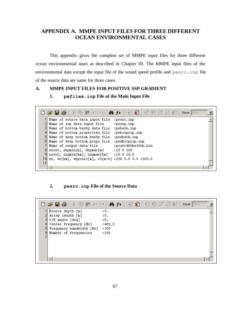
67

APPENDIX A. MMPE INPUT FILES FOR THREE DIFFERENT OCEAN ENVIRONMENTAL CASES

This appendix gives the complete set of MMPE input files for three different

ocean environmental cases as described in Chapter III. The MMPE input files of the

environmental data except the input file of the sound speed profile and pesrc.inp file

of the source data are same for three cases.

A. MMPE INPUT FILES FOR POSITIVE SSP GRADIENT

1. pefiles.inp File of the Main Input File

2. pesrc.inp File of the Source Data

D & *n r* /► gj ß Stack: p 2SJ

9

11

Name of source data input file Name of ssp data input file Name of bottom bathy data file Name of bottom properties file Name of deep bottom bathy file Name of deep bottom props file Name of output data file nz out, depmin[m], depmax[m] nr out, rngmin[km], rngmax[km] nz, dr[km], depcalcfm], cOfm/s]

<l

:pesrc.inp :pessp.inp :pebath.inp :pebotprop.inp :pedbath.inp :pedbotprop.inp :posfc400bw300b.bin :10 0 200 :10 0 10.0 :256 0.0 0.0 1500.0

ur

D ^ is m p o o. /► © £1 Sladc f" ~ 2<

1 [Source depth [m] 2 Array length [m] 3 D/E angle [deg] 4 Center frequency [Hz] 5 Frequency bandwidth [Hz]

Number of frequencies

5. D. 0. 400.0 300 256

iT

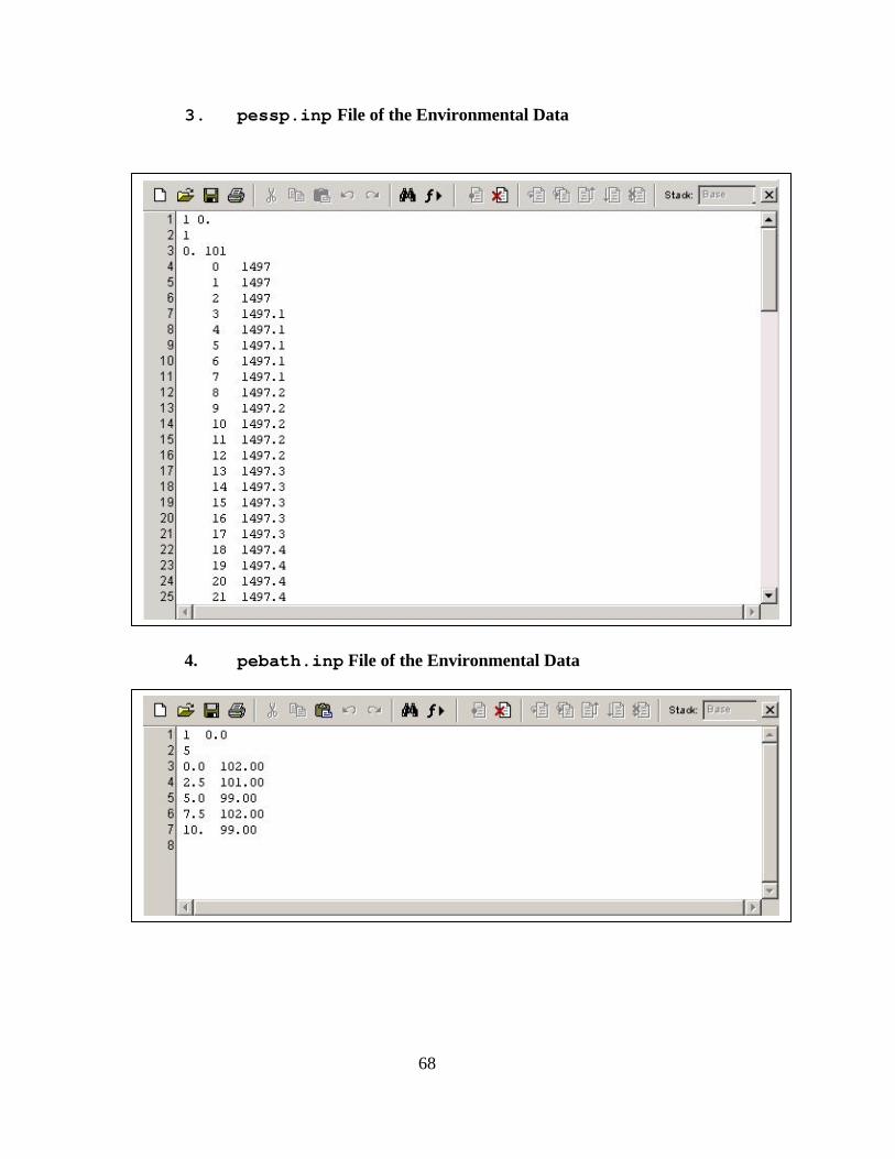
68

3. pessp.inp File of the Environmental Data

4. pebath.inp File of the Environmental Data

□ G£ H ß ^ ^ I M /► I © & I *u Stack ".*] 1 2

1 0. 1

3 0. 101 4 0 1497 5 1 1497 6 2 1497 7 3 1497.1 8 4 1497.1 S 5 1497.1

10 6 1497.1 11 7 1497.1 12 8 1497.2 13 9 1497.2 14 10 1497.2 15 11 1497.2 ie 12 1497.2 17 13 1497.3 18 14 1497.3 19 15 1497.3 2C 16 1497.3 21 17 1497.3 22 18 1497.4 23 19 1497.4 24 20 1497.4 25 21 1497.4

.

I S

D*I4 *U-|i^ ft /► gi <H 3ü IF JB € Stack: B ^XJ

1 1 0.0 5 0.0 102.00 2.5 101.00 5.0 99.00 7.5 102.00 10. 99.00

w I

<l

69

5. pebotprop.inp File of the Environmental Data

6. pedbath.inp File of the Environmental Data

7. pefiles.inp File of the Environmental Data

DG£H# IS «/►(♦H€l|1[i^][llTe©| Stadc: K X\

0. 1700. 1. 1.5 0.1 0. 0.

r

D & e m x % m « ^ #* /► MI ß hm © Uff © © sta* r i 0. 200.

liT

Dc*i«|x§iB«o. ;ä/>| ü ß | «ü © nr ü © st** [^ xJ

0. 200Q. 0. 3. 0.25 0. 0.

±] LT

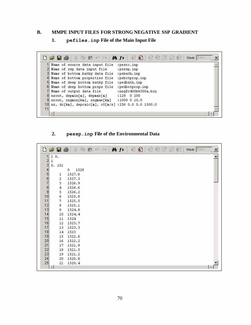
70

B. MMPE INPUT FILES FOR STRONG NEGATIVE SSP GRADIENT

1. pefiles.inp File of the Main Input File

2. pessp.inp File of the Environmental Data

D & S ft »a c* /► E ß Stack: :*l

9 10 11

Name o Name o Name o Name o Name o Name o Name o nzout, nrout, nz, dr

f source data input file f ssp data input file f bottom bathy data file f bottom properties file if deep bottom bathy file f deep bottom props file f output data file depmin[m], depmax[m] rngmin[km], rngmax[km]

[km], depcalc[m], c0[m/s]

iJ.

:pesrc.inp :pessp.inp :pebath.inp :pebotprop.inp :pedbath.inp :pedbotprop.inp :negfc400bra300a.bin :128 0 200 :1000 0 10.0 :256 0.0 0.0 1500.0

hT

□ & H H ä /► I @ fl 1 1 0. 2 1 3 0. 101 4 0 1528 5 1 1527.6 6 2 1527.3 7 3 1526.9 8 4 1526.6 9 5 1526.2

10 6 1525.8 11 7 1525.5 12 8 1525.1 13 9 1524.8 14 10 1524.4 15 11 1524 16 12 1523.7 17 13 1523.3 18 14 1523 19 15 1522.6 20 16 1522.2 21 17 1521.9 22 18 1521.5 23 19 1521.2 24 20 1520.8 25 21 1520.4

I ►r1

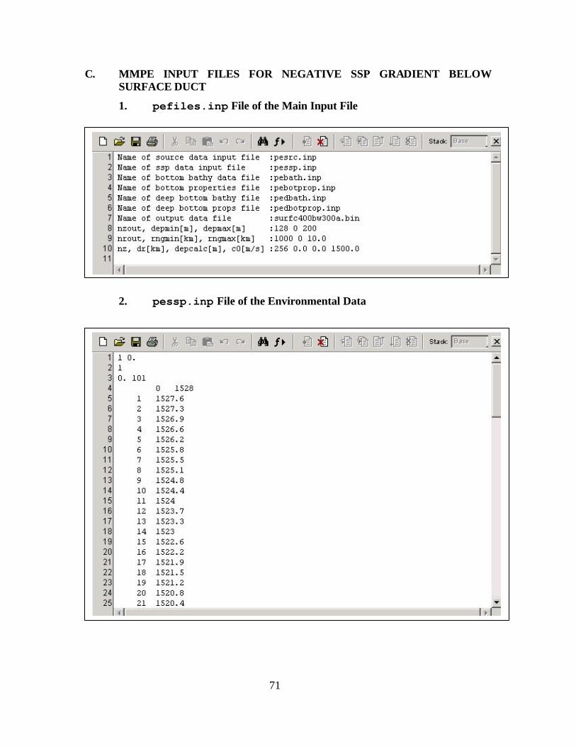
71

C. MMPE INPUT FILES FOR NEGATIVE SSP GRADIENT BELOW SURFACE DUCT

1. pefiles.inp File of the Main Input File

2. pessp.inp File of the Environmental Data

0 GS Q X in c* /► ß StJ*: r .-si 1 2 3 4 S 6 7 8 9

10 11

Name o Name o Name o Name o Name o Name o Name o nzout, nLOut, nz, dr

f source data inpuc file f ssp data input file f bottom bathy data file if bottom properties file f deep bottom bathy file f deep bottom props file f output data file depmin[m], depmax[m] mgmin[km], mgmax[km]

[km], depcalc[m], cO[m/s]

ipesrc.inp :pessp.inp ipebath.inp ipebotprop.inp ipedbath.inp ipedbotprop.inp :surfc400bu300a.bin :128 0 200 :1000 0 10.0 :2S6 0.0 0.0 1S00.0

Dc*H»|*Qife^^ « /► it m © if © © | «a* 2<

\

1 0. 1

A

3 0. 101 4 0 1S28 5 1 1527.6 6 2 1527.3 7 3 1526.9 —

8 4 1526.6 9 5 1526.2

10 6 1525.8 11 7 1525.5 12 8 1525.1 13 9 1524.8 14 10 1524.4 15 11 1524 16 12 1523.7 17 13 1523.3 18 14 1523 19 15 1522.6 20 16 1522.2 21 17 1521.9 22 18 1521.5 23 19 1521.2 24 20 1520.8 25 21 1520.4

72

THIS PAGE INTENTIONALLY LEFT BLANK

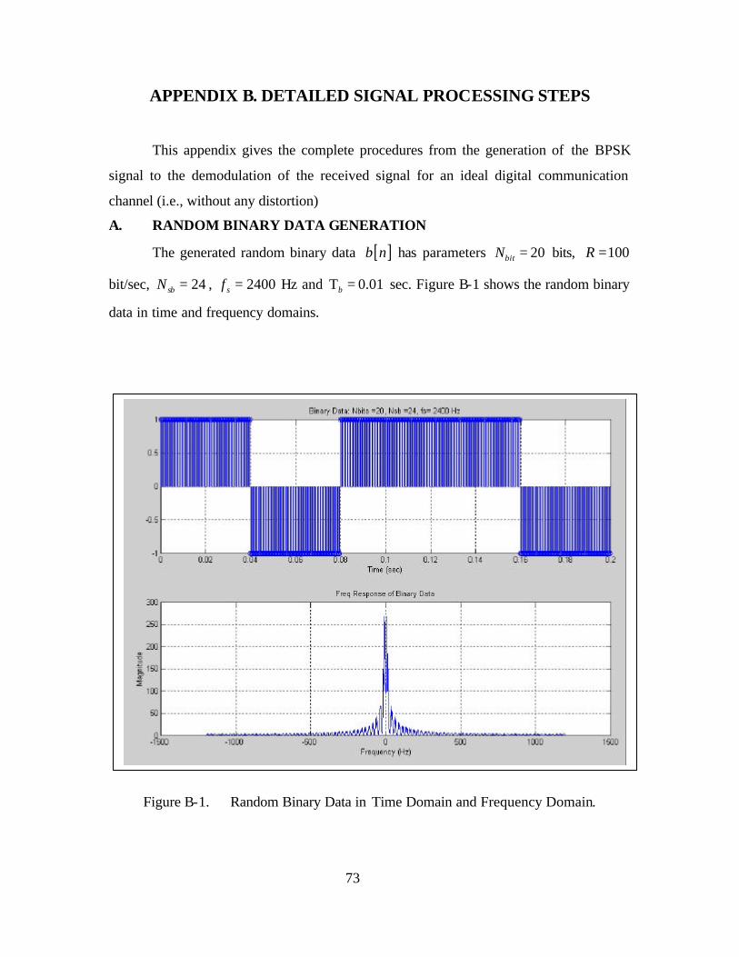
73

APPENDIX B. DETAILED SIGNAL PROCESSING STEPS

This appendix gives the complete procedures from the generation of the BPSK

signal to the demodulation of the received signal for an ideal digital communication

channel (i.e., without any distortion)

A. RANDOM BINARY DATA GENERATION

The generated random binary data [ ]b n has parameters 20bitN = bits, 100R =

bit/sec, 24sbN = , 2400sf = Hz and 0.01bΤ = sec. Figure B-1 shows the random binary

data in time and frequency domains.

Figure B-1. Random Binary Data in Time Domain and Frequency Domain.

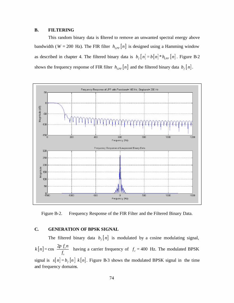
74

B. FILTERING

This random binary data is filtered to remove an unwanted spectral energy above

bandwidth ( 200W = Hz). The FIR filter [ ]LPFh n is designed using a Hamming window

as described in chapter 4. The filtered binary data is [ ] [ ] [ ]f LPFb n b n h n= ∗ . Figure B-2

shows the frequency response of FIR filter [ ]LPFh n and the filtered binary data [ ]fb n .

Figure B-2. Frequency Response of the FIR Filter and the Filtered Binary Data.

C. GENERATION OF BPSK SIGNAL

The filtered binary data [ ]fb n is modulated by a cosine modulating signal,

[ ] 2cos c

s

f nk n

fπ

=

having a carrier frequency of 400cf = Hz. The modulated BPSK

signal is [ ] [ ] [ ]fs n b n k n= ⋅ . Figure B-3 shows the modulated BPSK signal in the time and frequency domains.

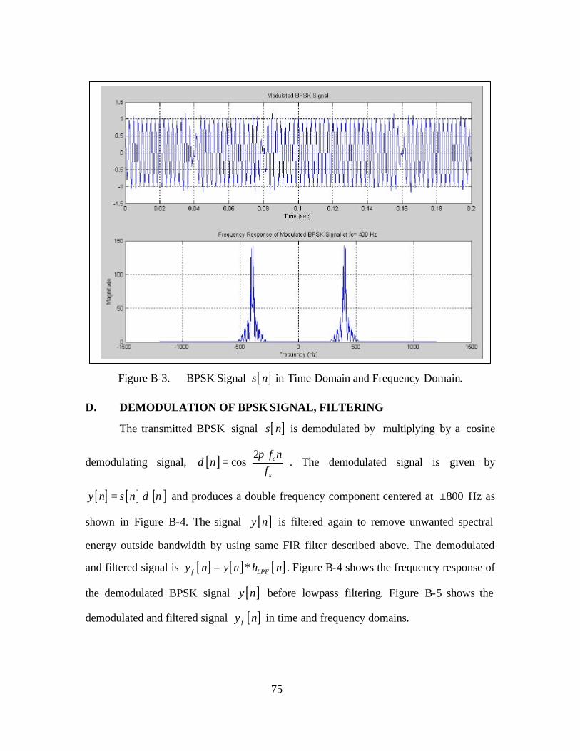
75

Figure B-3. BPSK Signal [ ]s n in Time Domain and Frequency Domain.

D. DEMODULATION OF BPSK SIGNAL, FILTERING

The transmitted BPSK signal [ ]s n is demodulated by multiplying by a cosine

demodulating signal, [ ] 2cos c

s

f nd n

fπ

=

. The demodulated signal is given by

[ ] [ ] [ ]y n s n d n= ⋅ and produces a double frequency component centered at 800± Hz as

shown in Figure B-4. The signal [ ]y n is filtered again to remove unwanted spectral

energy outside bandwidth by using same FIR filter described above. The demodulated

and filtered signal is [ ] [ ] [ ]f LPFy n y n h n= ∗ . Figure B-4 shows the frequency response of

the demodulated BPSK signal [ ]y n before lowpass filtering. Figure B-5 shows the

demodulated and filtered signal [ ]fy n in time and frequency domains.

1*0

ice -

SJ

-läLD

F(84u9flC) Response tf MrtiJ *ied BPSK Sigral si ic^ 4)0 Hl 1 1

..................... ..................... ...

i ! !

!

i Äi i -wW llvi j -10X •510 0 SO

FtB3JBTOT tH(] IJl«J -..-

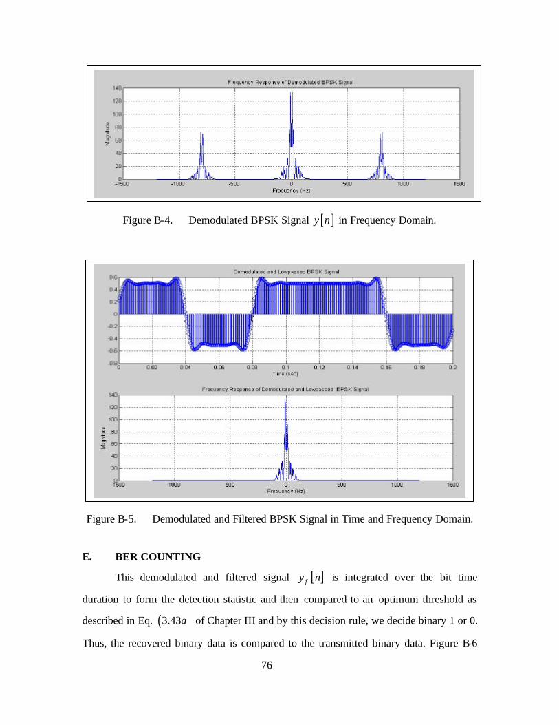
76

Figure B-4. Demodulated BPSK Signal [ ]y n in Frequency Domain.

Figure B-5. Demodulated and Filtered BPSK Signal in Time and Frequency Domain.

E. BER COUNTING

This demodulated and filtered signal [ ]fy n is integrated over the bit time

duration to form the detection statistic and then compared to an optimum threshold as

described in Eq. ( )3.43a of Chapter III and by this decision rule, we decide binary 1 or 0.

Thus, the recovered binary data is compared to the transmitted binary data. Figure B-6

1—i' I'll- ' -"' ■■■■: ■---.■■■!■; Sigi

■nil .- --*., mia ■.-.'... :i. .•- .. -1 . a.- ..■.-■ • I -■■' ■ : •

1JJ ■

10J -

i

;o

IOJL -... tOJ IXC ■ ,.. si ■ - ;■■:

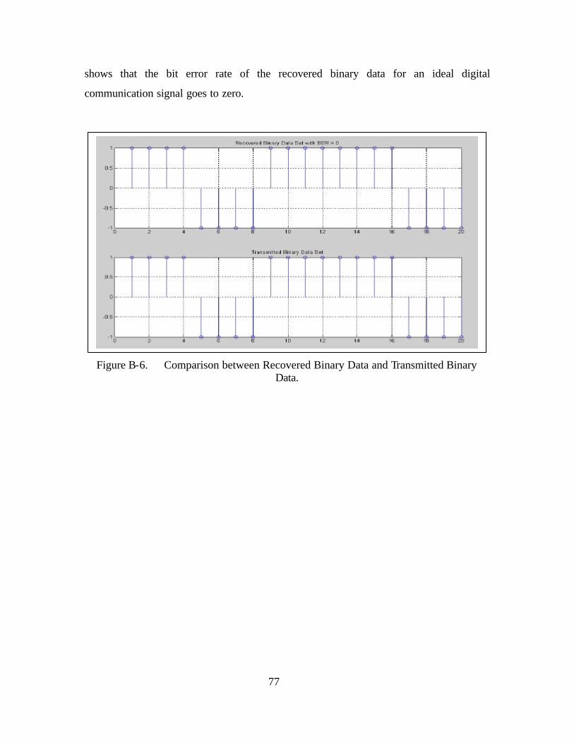
77

shows that the bit error rate of the recovered binary data for an ideal digital

communication signal goes to zero.

Figure B-6. Comparison between Recovered Binary Data and Transmitted Binary Data.

1

05

Rocc<o<6d Blnaiy Dais Sal ->(h BER = 0 '—■'—- —- ■— 1 | . . . . , , . ■ , , , j

'

i

.«.»i.» i i i *

^

i i i , i

i 1 2 4

r»— i 'SlE12

Ifadirtiniil Sifter) Data Stil

M Ü IS 2

1 r*

"""~

1

i— 1 — i j i !

i i i i i 4 -■—

0 10 13 14 ^ " <S' 3

78

THIS PAGE INTENTIONALLY LEFT BLANK

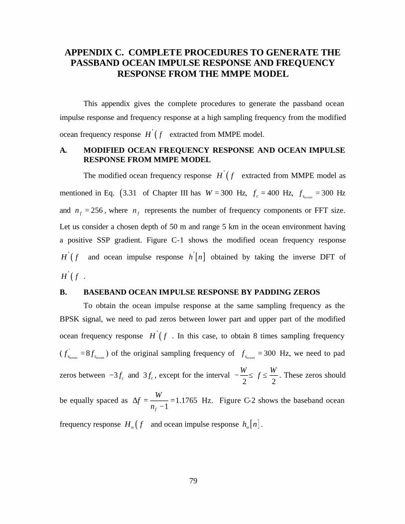
79

APPENDIX C. COMPLETE PROCEDURES TO GENERATE THE PASSBAND OCEAN IMPULSE RESPONSE AND FREQUENCY

RESPONSE FROM THE MMPE MODEL

This appendix gives the complete procedures to generate the passband ocean

impulse response and frequency response at a high sampling frequency from the modified

ocean frequency response ( )'H f extracted from MMPE model.

A. MODIFIED OCEAN FREQUENCY RESPONSE AND OCEAN IMPULSE RESPONSE FROM MMPE MODEL

The modified ocean frequency response ( )'H f extracted from MMPE model as

mentioned in Eq. ( )3.31 of Chapter III has 300W = Hz, 400cf = Hz, 300oceansf = Hz

and 256fn = , where fn represents the number of frequency components or FFT size.

Let us consider a chosen depth of 50 m and range 5 km in the ocean environment having

a positive SSP gradient. Figure C-1 shows the modified ocean frequency response

( )'H f and ocean impulse response [ ]'h n obtained by taking the inverse DFT of

( )'H f .

B. BASEBAND OCEAN IMPULSE RESPONSE BY PADDING ZEROS

To obtain the ocean impulse response at the same sampling frequency as the

BPSK signal, we need to pad zeros between lower part and upper part of the modified

ocean frequency response ( )'H f . In this case, to obtain 8 times sampling frequency

( ' 8ocean oceans sf f= ) of the original sampling frequency of 300

oceansf = Hz, we need to pad

zeros between 3 cf− and 3 cf , except for the interval 2 2

W Wf− ≤ ≤ . These zeros should

be equally spaced as 1.17651f

Wf

n∆ = =

− Hz. Figure C-2 shows the baseband ocean

frequency response ( )oH f and ocean impulse response [ ]oh n .

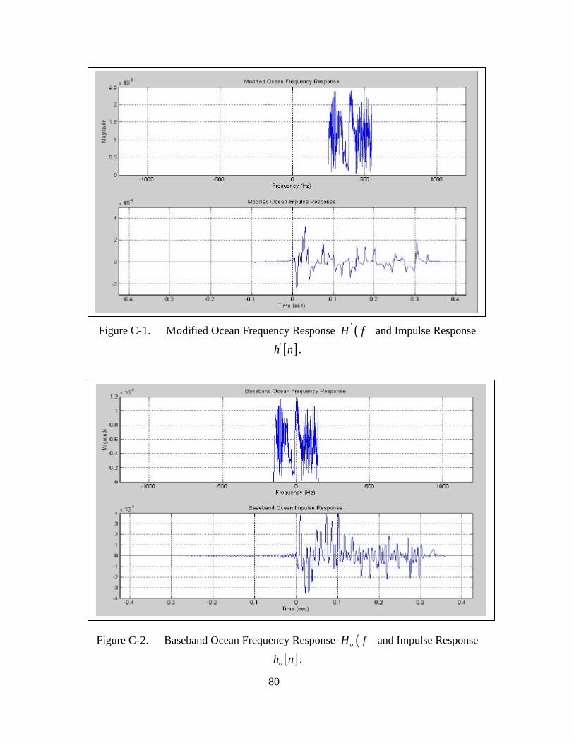
80

Figure C-1. Modified Ocean Frequency Response ( )'H f and Impulse Response

[ ]'h n .

Figure C-2. Baseband Ocean Frequency Response ( )oH f and Impulse Response

[ ]oh n .

MWilsd Oceo" Fiwiuc'icj' Renpsn

tffiJD

»10

•OT3 510 Frrswncy (Hz)

Mcmied Oces" h^uiee Responds

1COJ

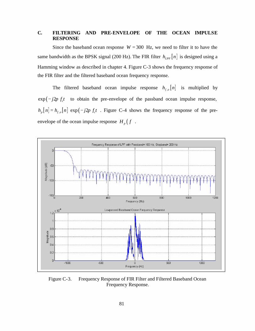
81

C. FILTERING AND PRE-ENVELOPE OF THE OCEAN IMPULSE RESPONSE

Since the baseband ocean response 300W = Hz, we need to filter it to have the

same bandwidth as the BPSK signal (200 Hz). The FIR filter [ ]LPFh n is designed using a

Hamming window as described in chapter 4. Figure C-3 shows the frequency response of

the FIR filter and the filtered baseband ocean frequency response.

The filtered baseband ocean impulse response [ ],f oh n is multiplied by

( )exp 2 cj f tπ− to obtain the pre-envelope of the passband ocean impulse response,

[ ] [ ] ( ), exp 2p f o ch n h n j f tπ= ⋅ − . Figure C-4 shows the frequency response of the pre-

envelope of the ocean impulse response ( )pH f .

Figure C-3. Frequency Response of FIR Filter and Filtered Baseband Ocean Frequency Response.

1.2 t ID Lowpesaefl Baseband Ocean Frequency Response

1 —

ii -•

-1QX -.J; Q Ftequency (Hi)

£00 1LCD

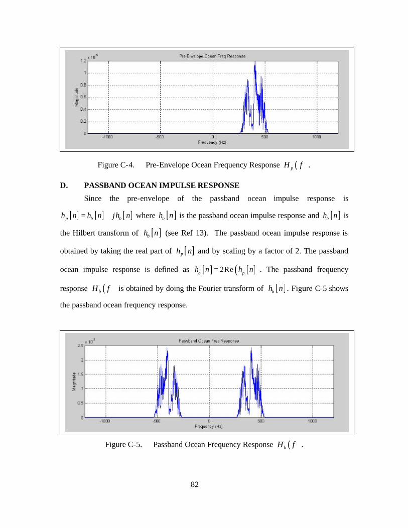
82

Figure C-4. Pre-Envelope Ocean Frequency Response ( )pH f .

D. PASSBAND OCEAN IMPULSE RESPONSE

Since the pre-envelope of the passband ocean impulse response is

[ ] [ ] µ [ ]p b bh n h n jh n= + where [ ]bh n is the passband ocean impulse response and µ [ ]bh n is

the Hilbert transform of [ ]bh n (see Ref 13). The passband ocean impulse response is

obtained by taking the real part of [ ]ph n and by scaling by a factor of 2. The passband

ocean impulse response is defined as [ ] [ ]( )2Reb ph n h n= . The passband frequency

response ( )bH f is obtained by doing the Fourier transform of [ ]bh n . Figure C-5 shows

the passband ocean frequency response.

Figure C-5. Passband Ocean Frequency Response ( )bH f .

25

2

1.5

. II Pr"ssi>ör;JOceän Fteq I

1 -

"- ■iam ■II gti iajD

Frequency (Hz)

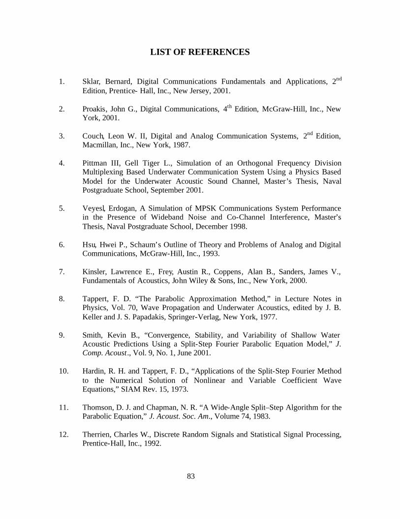
83

LIST OF REFERENCES

1. Sklar, Bernard, Digital Communications Fundamentals and Applications, 2nd Edition, Prentice- Hall, Inc., New Jersey, 2001.

2. Proakis, John G., Digital Communications, 4th Edition, McGraw-Hill, Inc., New

York, 2001. 3. Couch, Leon W. II, Digital and Analog Communication Systems, 2nd Edition,

Macmillan, Inc., New York, 1987. 4. Pittman III, Gell Tiger L., Simulation of an Orthogonal Frequency Division

Multiplexing Based Underwater Communication System Using a Physics Based Model for the Underwater Acoustic Sound Channel, Master’s Thesis, Naval Postgraduate School, September 2001.

5. Veyesl, Erdogan, A Simulation of MPSK Communications System Performance

in the Presence of Wideband Noise and Co-Channel Interference, Master’s Thesis, Naval Postgraduate School, December 1998.

6. Hsu, Hwei P., Schaum’s Outline of Theory and Problems of Analog and Digital

Communications, McGraw-Hill, Inc., 1993. 7. Kinsler, Lawrence E., Frey, Austin R., Coppens, Alan B., Sanders, James V.,

Fundamentals of Acoustics, John Wiley & Sons, Inc., New York, 2000. 8. Tappert, F. D. “The Parabolic Approximation Method,” in Lecture Notes in

Physics, Vol. 70, Wave Propagation and Underwater Acoustics, edited by J. B. Keller and J. S. Papadakis, Springer-Verlag, New York, 1977.

9. Smith, Kevin B., “Convergence, Stability, and Variability of Shallow Water

Acoustic Predictions Using a Split-Step Fourier Parabolic Equation Model,” J. Comp. Acoust., Vol. 9, No. 1, June 2001.

10. Hardin, R. H. and Tappert, F. D., “Applications of the Split-Step Fourier Method

to the Numerical Solution of Nonlinear and Variable Coefficient Wave Equations,” SIAM Rev. 15, 1973.

11. Thomson, D. J. and Chapman, N. R. “A Wide-Angle Split–Step Algorithm for the

Parabolic Equation,” J. Acoust. Soc. Am., Volume 74, 1983. 12. Therrien, Charles W., Discrete Random Signals and Statistical Signal Processing,

Prentice-Hall, Inc., 1992.

84

13. Ziomek, L. J., Fundamentals of Acoustic Field Theory and Space Time Signal Processing, CRC Press, Boca Raton, Fl, 1995.

85

INITIAL DISTRIBUTION LIST

1. Defense Technical Information Center Ft. Belvoir, Virginia

2. Dudley Knox Library Naval Postgraduate School Monterey, California

3. Prof. Kevin B. Smith, Code PH/SK Department of Physics

Naval Postgraduate School Monterey, California

4. Chairman, Code EC Department of Electrical and Computer Engineering

Naval Postgraduate School Monterey, California

5. Prof. Charles W. Therrien Department of Electrical and Computer Engineering

Naval Postgraduate School Monterey, California

6. Prof. Murali Tummala

Department of Electrical and Computer Engineering Naval Postgraduate School Monterey, California

7. LT Jung, Du San

Naval Postgraduate School Monterey, California