Final Report 2003-10 - Connect NCDOT · FINAL REPORT FHWA/NC/2004-12 in ... 2.1 Permeability 12 2.1.1 Constant Head and Falling Head Tests 12 2.2 Permeability in Pavements 14

DETERMINATION OF OPTIMUM GRADATION FOR RESISTANCE

TO PERMEABILITY,

RUTTING AND FATIGUE CRACKING

by

N. Paul Khoslaand

S. Sadasivam

HWY-2003-10

FINAL REPORTFHWA/NC/2004-12

in Cooperation with

North Carolina Department of Transportation

Department of Civil Engineering

North Carolina State University

February 2005

i

Technical Report Documentation Page

1. Report No.FHWA/NC/2004-12

2. Government Accession No. 3. Recipient’s Catalog No.

4. Title and SubtitleDetermination of Optimum Gradation for Resistance to Permeability,

5. Report Date02/28/2005

Rutting and Fatigue Cracking 6. Performing Organization Code7. Author(s)

N. Paul Khosla and S. Sadasivam8. Performing Organization Report No.

9. Performing Organization Name and AddressDepartment of Civil Engineering

10. Work Unit No. (TRAIS)

North Carolina State UniversityRaleigh, NC, 27695-7908

11. Contract or Grant No.

12. Sponsoring Agency Name and AddressNorth Carolina Department of TransportationResearch and Analysis Group

13. Type of Report and Period CoveredFinal Report2002-2004

1 South Wilmington StreetRaleigh, North Carolina 27601

14. Sponsoring Agency Code2003-10

15. Supplementary Notes:

16. Abstract

Permeability has become a major concern in recent years with the implementation of Superpave mixtures. It is important to havepavements that possess characteristics of low permeability which would minimize the effects due to moisture damage andincrease the service life of pavements. The permeability of mixtures mainly depends on percent air voids, nominal maximum sizeof aggregate and the type of gradation. At any given air void content or nominal size, the permeability depends on the size andcontinuity of air voids. The nature of gradation influences the size and continuity of voids. So the aggregate gradation wasoptimized for lower permeability without compromising the fatigue and rutting performance of mixtures. The application ofBailey method of gradation analysis showed that the permeability is greatly influenced by the aggregates of #4, #8 and # 16 sizes.Guidelines were proposed for the mix designers to arrive at aggregate blends with low or high permeability. The guidelinesrecommend a low proportion of #4 size aggregates and high proportion of #8 and # 16 size aggregates for low permeablemixtures. The higher proportions of 1/2" and 3/8" aggregates can be used to ensure the discontinuity of smaller voids. Theseguidelines were validated by permeability tests on a separate set of newly developed gradations.

The gradation and the binder content of the field cores were used to compact a reference mixture using the Superpave Gyratorycompactor in the laboratory. This reference mixture, the "unmodified gradation", is used for permeability tests and performanceanalysis. Four new mixtures were designed for both 12.5mm and 9.5mm mixtures in such a way that two mixtures had lowerpermeability and other two mixtures had higher permeability than the coefficient of the unmodified gradation. Performanceevaluation tests were conducted on field cores, the unmodified gradations, low permeable and high permeable mixtures beforeand after moisture damage. The performance evaluation tests included the Frequency Sweep Test at Constant Height, theRepeated Shear Test at Constant Height and the Asphalt Pavement Analyzer Test. The performance analysis indicated that thepermeability of the mixtures directly influences their performance in terms of fatigue life, rutting life and moisture susceptibility.The low permeable mixtures have higher fatigue life and rutting life than the high permeable mixtures. The low permeablemixtures have lower percent of reduction in service life due to moisture damage than the high permeable mixtures.

17. Key WordsPermeability, Gradations, Bailey Method, MoistureDamage, Superpave Mixture Performance.

18. Distribution Statement

19. Security Classif. (of this report)Unclassified

20. Security Classif. (of this page)Unclassified

21. No. of Pages141

22. Price

Form DOT F 1700.7 (8-72) Reproduction of completed page authorized

ii

DISCLAMIER

The contents of this report reflect the views of the authors and not necessarily the views of

the University. The authors are responsible for the facts and the accuracy of the data

presented herein. The contents do not necessarily reflect the official views or policies of

either the North Carolina Department of Transportation or the Federal Highway

Administration at the time of publication. This report does not constitute a standard,

specification, or regulation.

iii

ACKNOWLEDGMENTS

The author expresses his sincere appreciation to the authorities of the North Carolina

Department of Transportation for making available the funds needed for this research.

Sincere thanks go to Mr. Cecil Jones, Chairman, Steering and Implementation Committee,

for his interest and helpful suggestions through the course of this study. Equally, the

appreciation is extended to other members of the committee, Mr. Jack Cowsert, Mr. M.

Kadibhai, Mr. S. Sweitzer, Mr. Chris Bacchi, Dr. Judith Corley-lay, Mr. E. Powell, Mr. R.

Rochelle, Mr. .J. Phillips, Mr. L. Love for their continuous support during this study.

iv

TABLE OF CONTENTS

Chapter 1 Introduction 1

1.1 Background and Problem Statement 1

1.2 Objectives 4

1.3 Research Plan and Methodology 4

Chapter 2 Literature Review 12

2.1 Permeability 12

2.1.1 Constant Head and Falling Head Tests 12

2.2 Permeability in Pavements 14

2.3 Factors affecting Permeability Characteristics of Pavements 15

2.4 Critical Permeability Values 28

2.5 Permeability and Shear Strength 29

2.6 Correlation between Lab and Field Permeability values 29

2.7 Factors Influencing Lab Measurement of Permeability 30

2.8 Analysis of Gradations: A Background Study 31

Chapter 3 Optimization of Aggregate Gradations and

Permeability Tests of Mixtures 33

3.1 Bailey Method of Gradation Analysis 33

3.2 Trial Gradations 39

3.3 Permeability Apparatus and Test 40

3.4 Guidelines for Selecting Aggregate Gradations 50

3.4.1 Guidelines for 12.5mm Mixtures 51

3.4.2 Guidelines for 9.5mm Mixtures 54

3.5 Validation of Guidelines 56

Chapter 4 Asphalt Mixture Design 60

4.1 Field Specimens 60

4.2 Design of Asphalt Concrete Mixtures 61

v

4.2.1 Unmodified Gradation 61

4.2.2 Design of 12.5mm Mixtures 67

4.2.3 Design of 9.5mm Mixtures 70

Chapter 5 Performance Evaluation of Mixtures 73

5.1 Performance Evaluation using the Simple Shear Tester 73

5.2 Frequency Sweep Test at Constant Height 75

5.3 Analysis of FSCH Test Results 76

5.3.1 FSCH Test Results for 12.5mm Mixtures 76

5.3.2 FSCH Test Results for 9.5mm Mixtures 84

5.4 Repeated Shear Test at Constant Height 92

5.5 Analysis of RSCH Test Results 93

5.5.1 RSCH Test Results for 12.5mm Mixtures 93

5.5.2 RSCH Test Results for 9.5mm Mixtures 99

5.6 APA Rut Tests 104

Chapter 6 Performance Analysis of Mixtures 107

6.1 SUPERPAVE Fatigue Model Analysis 107

6.1.1 Fatigue Analysis of 12.5mm Mixtures 110

6.1.2 Fatigue Analysis of 9.5mm Mixtures 115

6.2 SUPERPAVE Rutting Model Analysis 119

Chapter 7 Discussion of Results and Conclusions 123

7.1 Discussion of Results 123

7.2 Conclusions 127

References 129

vi

LIST OF TABLES

Table No. Title Page

2.1 Typical Permeability Values for Different Nominal Maximum Sizes 18

2.2 Permeability Index for Different Gradations 22

2.3 Critical Permeability Values as Provided by AHTD Studies 28

2.4 Critical Permeability Values for Various Nominal Maximum Sizes 29

3.1 Control Sieves 38

3.2 Trial Gradations of 12.5mm Mixtures 41

3.3 Trial Gradations of 9.5mm Mixtures 42

3.4 Summary of Aggregate Ratios for 12.5mm Mixtures 43

3.5 Summary of Aggregate Ratios for 9.5mm Mixtures 43

3.6 Parameters used in Permeability Tests 47

3.7 Permeability Coefficients of 12.5mm mixtures 47

3.8 Permeability Coefficients of 9.5mm mixtures 48

3.9 Mixtures Selected for Performance Evaluation 49

3.10 Control Points for 12.5mm Mixtures 52

3.11 Control Points for 9.5mm Mixtures 54

3.12 Gradations of 12.5mm Mixtures for Validation 57

3.13 Gradations of 9.5mm Mixtures for Validation 57

3.14 Permeability Test Results 58

4.1 Mixture Properties of Field Cores 61

4.2 Unmodified Gradations 63

4.3 Combined Gradation and RAP 64

4.4 Volumetric Properties of 12.5mm Mixture with Unmodified Gradation 66

4.5 Volumetric Properties of 9.5mm Mixture with Unmodified Gradation 66

4.6 Percent Passing on Each Sieve (12.5mm Mixtures) 67

4.7 Compaction Criteria 69

4.8 Summary of Mix Design for Selected Gradations (12.5mm Mixtures) 69

4.9 Percent Passing on Each Sieve (9.5mm Mixtures) 70

4.10 Summary of Mix Design for Selected Gradations (9.5mm Mixtures) 72

vii


5.1 Frequency Sweep at Constant Height Test Results 77

(Field Cores and Unmodified)

5.2 FSCH Test Results (Low Permeable Mixtures) 77

5.3 FSCH Test Results (High Permeable Mixtures) 78

5.4 Comparison of |G*| @ 10Hz of 12.5mm Mixtures 81

5.5 Statistical Analysis of |G*| at 10 Hz for 12.5mm Mixtures 83

5.6 ANOVA Results for 12.5mm Mixtures (Unconditioned) 84

5.7 ANOVA Results for 12.5mm Mixtures (Conditioned) 84

5.8 Frequency Sweep at Constant Height Test Results 85

(Field Cores and Unmodified)

5.9 FSCH Test Results (Low Permeable Mixtures) 85

5.10 FSCH Test Results (High Permeable Mixtures) 86

5.11 Comparison of |G*| @ 10Hz of 9.5mm Mixtures 89

5.12 Statistical Analysis of |G*| at 10 Hz for 12.5mm Mixtures 91



5.15 RSCH Test Results of 12.5mm Mixtures 95

5.16 Statistical Analysis of Shear Strain for 12.5mm Mixtures 98



5.19 RSCH Test Results of 9.5mm Mixtures 100

5.20 Statistical Analysis of Shear Strain for 9.5mm Mixtures 103



5.23 APA Rut Depths of Unconditioned Specimens 105

5.24 APA Rut Depth of Conditioned Specimens 105

6.1 Summary of Estimated Material Properties for 12.5mm Mixtures 110

6.2 Fatigue Life Analysis of 12.5mm Mixtures 111

6.3 Summary of Fatigue Life of 12.5mm Mixtures (Nsupply) 112

viii


6.4 ANOVA Results for Fatigue Life of 12.5mm Mixtures (Unconditioned) 114

6.5 ANOVA Results for Fatigue Life of 12.5mm Mixtures (Conditioned) 114

6.6 Summary of Estimated Material Properties for 9.5mm Mixtures 115

6.7 Fatigue Life Analysis of 9.5mm Mixtures 116

6.8 Summary of Fatigue Life of 9.5mm Mixtures (Nsupply) 117

6.9 ANOVA Results for Fatigue Life of 9.5mm Mixtures (Unconditioned) 119

6.10 ANOVA Results for Fatigue Life of 9.5mm Mixtures (Conditioned) 119

6.11 Rut Depths of 12.5mm Mixtures 121

6.12 Rut Depths of 9.5mm Mixtures 121

ix

LIST OF FIGURES

Fig. No Figure Title Page

2.1 Constant Head Permeameter 13

2.2 Permeability vs Air Voids 17

2.3 Influence of Nominal Maximum Size of Aggregates on Permeability 18

2.4 Effect of Nominal Maximum Size on Field Permeability 19

2.5 Gradations used in Studies by Waddah Abdullah et al 21

2.6 Effect of Air Voids on Permeability for Different Gradations 22

2.7 Lab Permeability vs Ratio of Lift Thickness to NMAS 25

2.8 Relationship between Field Permeability Lift Thickness and Density 25

2.9 Relationship between Lab Permeability Lift Thickness and Density 26

2.10 Influence of Thickness of Asphalt Layer on Permeability 27

2.11 Relationships between Field and Lab Permeability Measurements 31

3.1 Division Points in Coarse and Fine Aggregate Fractions 35

3.2 Permeability Apparatus 45

3.3 Permeability Apparatus 46

3.4 Comparison of Permeability Coefficients (12.5mm Mixtures) 48

3.5 Comparison of Permeability Coefficients (9.5mm Mixtures) 49

3.6 Recommended Gradation Bands for 12.5mm Mixtures 53

3.7 Recommended Gradation Bands for 9.5mm Mixtures 55

3.8 Comparison of Permeability Coefficients for 12.5mm Mixtures 58

3.9 Comparison of Permeability Coefficients for 9.5mm Mixtures 59

4.1 Gradation Curve of 12.5mm Mixture 62

4.2 Gradation Curve of 9.5mm Mixture 62

4.3 Ignition Oven 64

4.4 Aggregate Leftover from Ignition Method 65

4.5 Gradation Curves for Low Permeable Mixtures (12.5mm Mixtures) 68

4.6 Gradation Curves for High Permeable Mixtures (12.5mm Mixtures) 68

4.7 Gradation Curves for Low Permeable Mixtures (9.5mm Mixtures) 71

4.8 Gradation Curves for High Permeable Mixtures (9.5mm Mixtures) 71

x

Fig. No Figure Title Page

5.1 Dynamic Modulus vs Frequency (Unconditioned Specimens) 78

5.2 Dynamic Modulus vs Frequency (Conditioned Specimens) 79

5.3 Phase Angle vs Frequency (Unconditioned Specimens) 79

5.4 Phase Angle vs Frequency (Conditioned Specimens) 80

5.5 Comparison of Dynamic Modulus at 10 Hz of 12.5mm Mixtures 82

5.6 Dynamic Modulus vs Frequency (Unconditioned Specimens) 86

5.7 Dynamic Modulus vs Frequency (Conditioned Specimens) 87

5.8 Phase Angle vs Frequency (Unconditioned Specimens) 87

5.9 Phase Angle vs Frequency (Conditioned Specimens) 88

5.10 Comparison of Dynamic Modulus at 10 Hz of 9.5mm Mixtures 89

5.11 RSCH Test Results for 12.5mm Mixtures (Unconditioned) 95

5.12 RSCH Test Results for 12.5mm Mixtures (Conditioned) 96

5.13 Comparison of Shear Strains of 12.5mm Mixtures 96

5.14 RSCH Test Results for 9.5mm Mixtures (Unconditioned) 100

5.15 RSCH Test Results for 9.5mm Mixtures (Conditioned) 101

5.16 Comparison of Shear Strains of 9.5mm Mixtures 101

5.17 Comparison of APA Rut Depths of Unconditioned Mixtures 105

6.1 Typical Pavement Structure and Loading 109

6.2 Fatigue Life of 12.5mm Mixtures 112

6.3 Fatigue Life of 9.5mm Mixtures 117

1

CHAPTER 1

INTRODUCTION

1.1 Background and Problem Statement

From 1988 to 1993, the Strategic Highway Research Program (SHRP) spent

approximately $50 million on research to develop new methods for specifying and

designing Hot Mix Asphalt. The result of this large research effort was a new mix design

system called "Superpave". Superpave included requirements for aggregates, asphalt

binders, and the compacted mixture. Checks and balances were included within the

Superpave mix design system to help ensure that the resulting pavements would be both

rut resistant and durable. One of the basic and important requirements of asphalt concrete

pavements is durability. Durability is critical to the long-term performance of asphalt

pavements as it reflects the ability of the mixture to resist weathering from air, water, and

solar radiation, as well as abrasion from traffic action. A recent review of the

performance of Superpave designed mixes conducted by National Center of Asphalt

Technology (NCAT) showed that they provide good resistance to rutting (1). However,

the review also indicated that there was a potential durability problem with some

Superpave mixtures.

Permeability of asphalt pavements has become a significant concern and an important

issue in recent years. Several states have expressed concerns that the Superpave designed

pavements are more permeable than pavements previously designed with the Marshall

Mix Design. If the mix is too permeable, premature stripping occurs, shortening the life

2

expectancy of the pavement. Permeability is a problem because the relatively coarser

nature of newer asphalt mixtures produces a greater number of interconnected voids,

allowing air and water to penetrate a pavement. Air increases the likelihood of oxidation

of the asphalt binder which can lead to pavement cracking. When water enters the

pavement structure, a variety of problems can result, including rutting and stripping, as

well as base and subgrade problems.

The amount of voids plays an important role in the durability of asphalt concrete

pavements and, in particular, in influencing the resistance to the action of air and water.

High voids make the pavement structure more permeable to air and water. High

permeability to water encourages stripping of the asphalt from the aggregate particles,

and endangering the subgrade layer and the base course as well. Low voids cause rutting

and shoving of asphalt mixtures. Low asphalt content, on the other hand, causes

pavements to ravel under the action of traffic. Voids content in an asphalt concrete

pavement can have a contrasting effect on its properties and performance. Therefore, the

voids must be carefully chosen so that none of the important characteristics are sacrificed.

The voids are directly related to the density of a mixture: thus, density must be closely

controlled to ensure that the initial in-place voids for dense-graded mixtures should be no

higher than eight percent and never fall below three percent during the life of the

pavement (2).

McLaughlin and Goetz surmised that permeability actually gives a better measure of a

pavement’s durability than does density (3). Permeability provides an indication of how

3

HMA will transmit water through the pavement, whereas density is just an indirect

measure of in-place air voids. As long as the voids are below eight percent, permeability

should not be a problem, but the permeability increases quickly as the void level exceeds

eight percent. It is important to realize that the permeability does not depend solely on the

total void content but also the nature of the voids in the mix. Mixtures of identical voids

content have significantly different permeability coefficients. Size and continuity of air

voids should be considered along with the total void content. Large size air pockets are

associated with coarse graded mixes, and the larger the air pockets, the greater the

possibility to obtain continuity between them. Once the continuity is established, water

can easily flow through these connected voids, and eventually causes serious damage to

the asphalt pavement layer and the layers underneath it. The permeability of a mixture

depends on the aggregate gradation and the compaction level.

With the new Superpave mix design system in use today, more and more coarse graded

mix designs are being used. Superpave mixtures are said to have a different void

structure than the conventional dense graded mixtures. It is believed that the air voids

within the Superpave mixtures are larger in size than the conventional dense graded

mixtures if both are compacted to the same air void content. Since the voids are larger,

there are more interconnected voids in the pavement layers, causing higher permeability.

These permeable pavements allow water to pass through them and cause premature

failures. Thus it is important that gradation be developed for surface course mixtures

which are coarser in nature with fewer interconnected voids so that their performance is

not affected by the moisture damage.

4

1.2 Objectives

The primary objectives of this study were to

1. Select several 12.5mm and 9.5mm mixtures with gradations on the coarser side and

review their void structure and permeability characteristics.

2. Modify the gradations in (1) above, using the Bailey Method to arrive at the desired

void structure.

3. Evaluate the gradations developed in (2) above in terms of permeability and

recommend a gradation band that will have different permeability levels.

4. Evaluate the effect of permeability on the performance characteristics of mixtures,

e.g. rutting and fatigue characteristics.

5. Evaluate the effect of moisture damage on performance characteristics of mixtures

such as fatigue life and rutting.

1.3 Research Plan and Methodology

The research plan had the following four main tasks:

1. The field sites were selected in consultation with NCDOT from which test samples

were collected.

2. The void structure and permeability characteristics of the field cores were evaluated.

Modifications in aggregate gradation were made to alter the void structure and

permeability of the field mixtures to minimize the moisture damage as well as help in

maintaining the high quality performance of the pavements. A band of gradation for

both 12.5mm and 9.5mm mixtures was proposed for arriving at different permeability

levels.

5

3. The performance characteristics were evaluated that included parameters from

Repeated Shear at Constant Height (RSCH) tests and Frequency Sweep at Constant

Height (FSCH) tests for both unconditioned and conditioned specimens.

Task 1: Field Site Selection and Test Material Procurement

The location and the total number of test sites were selected after consultation with

NCDOT. Ideally, these sites were the pavements that contain SUPERPAVE

volumetrically designed mixtures being used in either new or overlay constructions.

These test sites typically had coarser gradations of 12.5mm and 9.5mm nominal

maximum size of aggregate (NMSA) with high permeability. The mixture information

including gradations and mix designs were obtained. The field cores from these sites as

well as the raw materials used in these field sections were procured for further analysis in

the laboratory.

Task 2.1: Modification of Gradations

The concepts of Bailey Method of Gradation Evaluation were used to modify the

gradations of 12.5 and 9.5mm field mixtures to have a coarser aggregate structure but

with fewer interconnected voids or low permeability. Voids in an asphalt mixture, which

are fundamental in mixture design, are greatly influenced by changes in the volume

percentage of coarse aggregate in the mixture. Permeability of a mixture depends not

only on the VMA but also on the size and interconnectivity of the voids. Changing the

gradation of the coarse aggregate changes the size of the voids in the coarse aggregate, in

turn affecting the resulting VMA in the mixture. The aggregate ratios play an important

6

role in the modification of the nature of gradations. Based on the concepts provided by

the Bailey’s method, the aggregate gradations were modified for different levels of

permeability.

Task 2.2: Evaluation of Permeability Characteristics

Permeability can be defined as the property of a material which permits the passage of

fluids through the pores. The permeability characteristics of pavements are based on the

Darcy’s empirical law that was established for fine grained soils. The seepage of water

through pavements is characterized by the parameter “Darcy Coefficient of Permeability

(k)”. Two general approaches are used to measure permeability of a material using

Darcy’s law: a constant head test and a falling head test. The falling head test is generally

applied for studying the permeability characteristics of pavement cores. The falling head

test involves determining the amount of head loss through a given sample over a given

time. For the falling head test, the coefficient of permeability is calculated as follows:

k = (a L / At) * ln(h1/h2)

where

k = coefficient of permeability

a = area of stand pipe

L = length of sample

A = cross-sectional area of sample

t = time over which head is allowed to fall

h1= water head at beginning of test

h2 = water head at end of test

7

Literature suggests that for asphalt mixtures, the falling head test apparatus is better

suited than the constant head test apparatus (4). The constant head apparatus does not

allow the low-pressure differentials necessary to measure water flow in semi-porous

mixtures. However, for open-graded friction courses, a constant head permeability test

may be more appropriate.

Therefore, the falling head permeability test was chosen for this study. The test procedure

followed to the “Florida Method of Measurement of Water Permeability of Compacted

Asphalt Paving Mixtures” currently used by NCDOT (5).

Task 3: Performance Evaluation

The performance testing and performance prediction models are important in designing

and managing pavements. The mixtures with modified gradations using the Bailey’s

method were evaluated for its performance characteristics using the APA and the SST.

Task 3.1: Asphalt Pavement Analyzer

The rutting susceptibility of the mixtures was assessed by placing samples under

repetitive loads of a wheel-tracking device, known as Asphalt Pavement Analyzer (APA).

APA is the new generation of the Georgia Loaded Wheel Tester (GLWT). The APA has

additional features that include a water storage tank and is capable of testing both

gyratory and beam specimens. The APA basically consists of three parallel steel wheels,

rolling on a pressurized rubber tube, which applies loading to beam or cylindrical

8

specimens in a linear track. The test specimens, loading tubes and wheels are all

contained in a thermostatically controlled environmental chamber. The depth of rutting in

the test specimens was measured after the application of 8000 loading cycles.

Task 3.2: Simple Shear Tester

The SST is a closed-loop system that consists of four major components such as the

testing apparatus, the test control unit and data acquisition system, the environmental

control chamber, and the hydraulic system. In this study, repeated shear test at constant

height and frequency sweep test at constant height were used to analyze the performance

of HMA mixtures. A full description of the test procedures can be found in AASHTO

TP7. The rutting and fatigue analyses were conducted using the test results.

The frequency sweep test at constant height was used to analyze the permanent

deformation and fatigue cracking. A repeated shearing load was applied to the specimen

to achieve a controlled shearing strain of 0.05 percent. The specimen was tested at each

of the following loading frequencies: 10, 5, 2, 1, 0.5, 0.2, 0.1, 0.05, 0.02 and 0.01 Hz. The

dynamic shear modulus G* and phase angle φ were determined by this test.

The repeated shear test at constant height was performed to identify an asphalt mixture

that is prone to tertiary rutting. Tertiary rutting occurs at low air void contents and is the

result of bulk mixture instability. In this test, repeated synchronized shear and axial load

were applied to the specimen. The test specimens were subjected to load cycles of 5000

cycles or until the permanent strain reached five- percent. One load cycle consists of 0.1-

9

second load followed by 0.6-second rest period. The permanent shear strains were

measured in this test.

Task 3.3: Analysis of the Service Life of the Pavement Structure

The resulting parameters of FSCH and RSCH tests are the material responses that can be

used to predict the pavement’s performance under service for distresses such as fatigue

cracking and rutting. Fatigue and rutting analysis were performed using surrogate

models developed by SHRP 003-A project. Fatigue analysis of SHRP model considers

material properties as well as pavement structural layer thickness whereas rutting analysis

considers only the material properties. Such a rutting and fatigue analysis of

representative pavement sections was performed. A brief summary of the procedure for

rutting and fatigue analysis is presented in the following sections.

Task 3.3.1: Fatigue Analysis

Fatigue distress is a function of and dependent on both mixture properties as well as the

pavement structural layer thickness. The fatigue analysis procedure requires an estimate

of the flexural stiffness modulus (So) of the asphalt-aggregate mix at the desired

temperature. In this investigation, it is assumed that the effective temperature for fatigue

cracking is 20o C. This estimated flexure stiffness was used in the multilayered elastic

analysis to determine the critical strain to which asphalt concrete mixture will be

subjected under a standard traffic loading. The critical strain was then used to compute

fatigue life of the mixture.

10

The flexural properties of mixtures were estimated from the RSCH tests using the

following equations:

So = 8.560(Go)0.013

So" = 81.125 (Go") 0.725

where,

So = flexural stiffness in psi

Go = dynamic shear stiffness at 10Hz in psi

So" = flexural loss stiffness in psi, and

Go" = dynamic shear loss stiffness at 10 Hz in psi

The critical tensile strain (εo) under the asphalt concrete layer was evaluated. The

following equation is used to evaluate the laboratory fatigue resistance of the asphalt mix.

Nsupply = 273800 * e (0.077.VFA) * (εo)-3.624 * (So") -2.720

where,

Nsupply = the number of E18 load repetitions to laboratory fatigue cracking,

εo = critical tensile strain,

So" = the flexural loss stiffness in psi, and

VFA = the voids filled with asphalt in percent.

Task 3.3.2: Rutting Analysis

The rut depth is calculated using the following relationship:

Rut Depth (in.) = 11 x (γp)

where,

11

γp= the maximum permanent shear strain in the RSCH test.

The conversion of the number of RSCH cycles to ESALS is done as follows:

Log (Cycles) = -4.36 + 1.24 log (ESALs)

The rut depths were estimated from the shear strains of RSCH tests using the above

equations.

12

CHAPTER 2

LITERATURE REVIEW

In this chapter, the earlier research studies about the permeability characteristics of the

asphalt pavements are discussed. The theory of permeability and the various factors

influencing permeability are discussed. The Bailey method of gradation analysis is also

described in this chapter.

2.1 Permeability

Permeability can be defined as the ability of a porous medium to transmit fluid. Based on

Darcy’s studies, the fundamental theory of permeability for soils was established. He

showed that the rate of water flow was proportional to the hydraulic gradient and area of

a sample. The hydraulic gradient is a very important concept when evaluating

permeability. It can be defined as the head loss per unit length. The head loss increases

linearly with the velocity of water transmitted through a medium as long as the flow of

water is laminar. Once the flow of water becomes turbulent, the relationship between

head loss and velocity is nonlinear. Thus in a turbulent water flow condition, Darcy’s law

is invalid (6). Two general approaches are used to measure permeability of a material

using Darcy’s law: a constant head test and a falling head test.

2.1.1 Constant Head and Falling Head Tests

The constant head test with soils testing setup similar to that described in ASTM D 5084

was used, as shown in Figure 2.1. The 152-cm-diameter specimen was enclosed in a

13

rubber membrane with porous stones at the top and bottom. The specimen was then

placed in a cell, and water was used to apply a confining pressure. Both the inlet pressure

and outlet pressure could be controlled on the water as it flowed through the length of the

specimen. It was desirable to have low differential pressure so as not to get turbulent flow

(4).

Figure 2.1 Constant Head Permeameter

The coefficient of permeability was calculated according to the following formula:

=

AthQL

k

where

k = permeability, cm/s

Q = quantity of flow, cm3

L = length of specimen, cm

A = cross-sectional area of specimen, cm2

t = interval of time over which flow Q occurs, s

h = difference in hydraulic head across the specimen, cm.

14

The falling head test involves determining the amount of head loss through a given

sample over a given time. This type of test is more suitable for less permeable materials

(4).

For the falling head test, the coefficient of permeability is calculated as follows:

k = (a L / At) * ln(h1/h2)

where

k = coefficient of permeability

a = area of stand pipe

L = length of sample

A = cross-sectional area of sample

t = time over which head is allowed to fall

h1= water head at beginning of test

h2 = water head at end of test

2.2 Permeability in Pavements

Within the hot mix asphalt community, it is generally accepted that the proper

compaction of HMA is vital for a stable and durable pavement. For dense-graded

mixtures, numerous studies have shown that initial in-place air void contents should not

be below 3 percent or above approximately 8 percent. Low air voids have been shown to

lead to rutting and shoving, while high air voids are believed to allow water and air to

penetrate into the pavement resulting in an increased potential for moisture damage,

raveling, and/or cracking.

15

In the past, it has been thought that for most conventionally designed dense-graded HMA

(Hveem and Marshall), increases in in-place air void contents have meant increases in

permeability. Zube showed that dense-graded HMA pavements become highly permeable

to water at approximately 8 percent air voids (7). Figure 2.2 shows that as long as the

voids are below 8 percent, permeability should not be a problem, but the permeability

increases quickly as the void level exceeds 8 percent. Brown, Collins and Brownfield, in

a study of segregated mixes in Georgia, also showed that HMA mixtures are

impermeable to water as long as the air void content was below approximately 8 percent

(8). Figure 2.2 shows that permeability increases rapidly at voids content above 8 percent.

However, due to problems associated with some coarse-graded Superpave designed

mixes in Florida (gradation passing below maximum density line and restricted zone), the

size and interconnectivity of the air voids have been shown to greatly influence pavement

permeability(9). The problems encountered with coarse-graded Superpave mixes in

Florida and elsewhere have put a high emphasis on the permeability testing of HMA

pavements. This is likely due to permeability giving a better indication of a pavement’s

durability than density alone.

2.3 Factors affecting Permeability Characteristics of Pavements

Permeability in hot mix asphalt pavements is not a new problem. However, since the

adoption of the Superpave mix design system the problem has gotten a lot of publicity.

Numerous studies have been conducted to identify and investigate the factors affecting

16

permeability characteristics of pavements. The findings of earlier research are compiled

here. A number of mixture and construction factors seem to significantly affect the

permeability characteristics of pavements. The major factors that affect the permeability

characteristics are as follows:

• Air voids

• Nominal Maximum Size of the Aggregate (NMAS)

• Gradation of Aggregates (above or below the Maximum Density Line)

• Lift Thickness

• Roller type

• Time of Construction

Air voids:

The prominent factor that affects the permeability of a pavement is the air voids.

Numerous studies have reported that the permeability increases with increasing air voids.

A pronounced increase in the permeability is observed when the air voids level of the

pavement increases above 8 percent. Choubane et al found that there was no significant

change in permeability when the amount of air voids falls below seven percent (9). The

researchers recommended an air void content of 6 percent or less for an impervious

coarse-graded Superpave pavement. Cooley et al found a strong relationship between the

permeability and in-place air voids (10). Studies by Mallick et al confirmed the influence

of air voids on the permeability, as shown in Figure 2.2 (11).

17

Figure 2.2 Permeability vs Air Voids

Nominal Maximum Size of Aggregate (NMAS):

The permeability of pavements has a direct relationship with the nominal sizes of the

aggregates. As the NMAS increases, the size of air voids within a pavement also likely

increases, especially in coarse graded Superpave mixes. As the size of voids increases,

the potential for interconnected air voids also increases. The in-place permeability of

pavements is directly related to the amount of interconnected voids. Therefore, as the

NMAS increases the air void level at which a pavement becomes excessively permeable

would be expected to decrease.

Permeability Studies by Mallick et al (11) show the change of permeability

characteristics with an increase in NMAS, as shown in Figure 2.3. The figure clearly

shows that permeability increases with increasing NMAS and so do the in-place air voids.

18

The authors provide an instance of permeability values for different nominal sizes at an

in-place air void level of 6 percent, as shown in Table 2.1.

Table 2.1 Typical Permeability Values for Different Nominal Maximum Sizes

NMAS mm Permeability, cm/sec

9.5

12.5

19.0

25.0

6 x 10-5

40 x 10-5

140 x 10-5

1200 x 10-5

Figure 2.3 Influence of Nominal Maximum Size of Aggregates on Permeability

19

Another study by Cooley et al confirms the effect of NMAS on permeability (12). The

authors found that at a given air void content, the 19.0 mm NMAS mixes showed

significantly higher permeability values than the 9.5 and 12.5 mm NMAS mixes. Also,

the 25.0 mm NMAS mixes had about three times higher permeability value than the 19.0

mm NMAS mixes at the same air void content. The results are illustrated in Figure 2.4.

So the nominal maximum aggregate size of the mix affects the permeability

characteristics of a pavement. Mixes having larger nominal maximum aggregate sizes

have a potential for high permeability.

Figure 2.4 Effect of Nominal Maximum Size on Field Permeability

20

Gradation:

Another factor that affects permeability characteristics is a mixture’s gradation shape.

Gradations that pass below the maximum density line (MDL) tend to become excessively

permeable at lower in-place air void contents than mixes having gradations that pass on

the fine side of the MDL. Similar to NMAS, gradation shape likely affects the size of the

air voids within a compacted pavement. Coarser gradations contain a higher percentage

of coarse aggregate which results in larger individual air voids and, thus, a higher

potential for interconnected air voids.

One of the earlier papers that dealt with the influence of gradation on permeability

characteristics is “Influence of Aggregate Type and Gradations on Voids of asphalt

Concrete Pavements” by Waddah Abdullah et al (13). The researchers used three

aggregate types and five gradations in their study. The three gradations were crushed

limestone, crushed basalt and crushed granite. As shown in Figure 2.5, the five gradations

were as follows:

• ASTM upper limit

• ASTM lower limit

• ASTM middle limit

• Gradation within the ASTM, designated as “A”

• Gradation obtained by Lees’ rational method, designated as “rational”

21

Figure 2.5 Gradations used in Studies by Waddah Abdullah et al

Water permeability studies showed that the coefficient of permeability of a specific

asphalt concrete mix yields more or less a straight line relationship with air voids in the

mix when plotted as “log10 k (permeability coefficient) vs. air content” in that mix. The

test results showed that asphalt concrete mixtures prepared with the ASTM lower limit

gradation and the A-gradation yielded the highest permeability values for the three types

of aggregates. Asphalt concrete mixtures prepared by Lees rational gradation yielded the

lowest values of permeability for the types of aggregates. The results showed that the

permeability values were influenced by the size of the voids and voids content itself.

The water permeability index Iwk was calculated for the combinations of the aggregate

types and gradations, as shown in Table 2.2. The index Iwk is defined as follows:

Iwk = dlog10 K/dAv

The rate of increase of the coefficient of permeability with increasing voids in the mix is

not the same for asphalt mixes made with different aggregate gradations. The coarser the

mix, the higher the rate of increase and vice versa. This behavior is attributed to the fact

22

that asphalt mixes, based on coarse gradations, have large size void sizes. The more the

air voids of this kind, the more the connectability of these voids, thus giving rise to large

diameter conduits for water to flow through them.

Figure 2.6 Effect of Air Voids on Permeability for Different Gradations

Table 2.2 Permeability Index for Different Gradations

(Studies by Waddah Abdullah et al)

Permeability index for Different Gradations.Type of

Aggregate Rational A Upper Middle Lower

Limestone 0.017 0.301 0.10 0.143 0.301

Granite 0.114 0.43 0.065 0.178 0.449

Basalt 0.04 0.37 0.10 0.174 0.484

23

Lift Thickness:

A construction issue that could also affect permeability is the lift thickness at which a

pavement is placed. As the lift thickness increases, the potential for permeability is likely

to decrease. There are two reasons for lift thickness to make a difference. First, thicker

lifts are generally easier to compact in the field because a thicker lift retains heat better

and allows more room for aggregate particles to orientate properly; hence, an increase in

pavement density. Secondly, permeability is the result of interconnected voids. Within

dense-graded hot mix asphalt, all air voids are not interconnected. As lift thickness

increases, the chance for voids being interconnected with a sufficient length to allow

water to flow decreases. For this reason, thinner pavements may have more potential for

permeability.

As with soils, HMA permeability is directly related to the amount of interconnected voids

within the pavement. The interconnected voids are the conduits through which water

flows. However, unlike soils all voids within HMA pavements are not interconnected.

Take for instance a pavement that is 50 mm thick. A single interconnected air void may

exist that allows water to flow through the pavement. If the same pavement is 75 mm

thick, it is not necessarily true that the same interconnected air void will exist throughout

the entire pavement since all air voids are not interconnected.

A study by Mallick et al shows that the thicker pavements are less permeable (11).

Figure 2.7 illustrates that the permeability of asphalt pavements is related the thickness of

samples. This figure present the results of the laboratory experiment conducted on lab

24

compacted loose mix from three of the five projects. The projects include the coarse

graded 9.5 mm, 12.5 mm, and 19.0 mm NMAS mixtures. This figure shows that as the

thickness increases (or thickness to NMAS ratio increases), the permeability also

decreases. At a thickness to NMAS (t/NMAS) ratio of 2.5, all three mixes exhibit the

largest permeability value. Likewise, at the t/NMAS ratio of 4, all mixes had the lowest

permeability value. The 12.5 mm NMAS mix did show an anomaly at the 3.5:1 t/NMAS

ratio in that the permeability was higher than at the 3 t/NMAS ratio. However, the

permeability did again decrease at the t/NMAS ratio of 4. Even with the anomaly, the

data clearly shows that the thicker pavements should be less permeable.

Another study by Cooley et al on the issues pertaining to the permeability characteristics

of coarse graded mixtures proved that the field permeability is a function of lift thickness

and density (12). A multiple linear regression was performed to relate permeability to

density, thickness and nominal size. The relationships for field permeability and

laboratory permeability with R2 values of 0.66 and 0.51, respectively, are shown below:

Ln(Field Permeability) = -1.787 + 0.592(Air Voids) + 0.196(NMAS) - 0.23(t/NMAS)

Ln(Lab Permeability) = -5.335 + 4.61*Ln(Air Voids) + 0.138(NMAS) - .024(Thickness)

Figures 2.7, 2.8 and 2.9 illustrate the results of multiple linear regression for field as well

as laboratory data.

25

Figure 2.7 Lab Permeability vs Ratio of Lift Thickness to NMAS

Figure 2.8 Relationship between Field Permeability Lift Thickness and Density

26

Figure 2.9 Relationship between Lab Permeability Lift Thickness and Density

A study by Arkansas State Highway and Transportation department shows that the

permeability coefficient k decreases with increasing lift thickness as shown in Figure

2.10 (13). They developed a regression equation that related permeability coefficient with

in-place air voids and thickness. The regression equation (R2 = 0.748) is shown below:

k = (1.38 x 10-7) (3.92%AV) (0.61Lift Thickness)

The study recommended that the minimum lift thickness should be greater than 2 inches

or 4 times the maximum nominal aggregate size.

27

Figure 2.10 Influence of Thickness of Asphalt Layer on Permeability

Roller Type:

Another construction issue that may influence permeability is roller type. Work by

Cechetini has suggested that the type of roller and rolling pattern during construction can

affect pavement permeability (14). According to Cechetini, vibratory rollers reduce the

potential for permeability. Also, there was a suggestion in the past that the use of

pneumatic tire rollers may decrease the potential for permeable pavements. Pneumatic

rollers tend to knead the pavement during compaction which may reduce the potential for

interconnected voids.

Time of Construction:

Zube found that the time of the construction will affect the permeability characteristics

(7). Pavements constructed in the spring can be expected to “seal up” due to the summer

traffic thus reducing the permeability better than if the mix was placed in the fall.

Pavements constructed in the fall may not “seal up” due to cooler weather and lead to

28

permeability problems for an extended time period. This is a valid point and shows why a

fixed “paving season” is essential to quality pavements.

2.4 Critical Permeability Values

Few research studies have drawn up certain guidelines for categorizing pavement

sections according to the permeability values of their representative cores. The University

of Arkansas as part of the AHTD’s Transportation Research Project No. 82, "Asphalt

Mix Permeability" categorizes as shown in Table 2.3. The above classification is

categorized only on the permeability coefficients, irrespective of the NMAS and density.

Table 2.3 Critical Permeability Values as Provided by AHTD Studies

Permeability Category Permeability Rates

High Permeability 101-10-4

Low Permeability 10-4-10-6

Practically Impervious 10-6-10-9

In a research study at NCAT, Cooley et al developed critical values of permeability

taking the pavement density and nominal size into account (15). Table 2.4 furnishes the

critical values of permeability and pavement density for various nominal sizes such as

9.5mm, 12.5mm, 19.0mm and 25.0 mm. The term “critical” used in that study inferred

the point at which a pavement becomes excessively permeable. For the larger NMAS

mixes, some permeability may be acceptable as long as the upper layers are impermeable.

29

Table 2.4 Critical Permeability Values for Various Nominal Maximum Sizes

NMAS, mm Permeability, cm/sec Density

9.5 100 x 10-5 92.3 %

12.5 100 x 10-5 92.3%

19.0 120 x 10-5 94.5%

25.0 150 x 10-5 95.6%

2.5 Permeability and Shear Strength

Kentucky Transportation Center investigated a pavement section which had permeability

related problems (16). The field permeability tests showed that in the areas and locations

where the mat failed to meet density requirements exhibited very high permeability in

those locations. When the direct shear tests were performed on these cores, the results

showed a direct relationship between maximum shear strength and density. The authors

concluded that nearly all of the laboratory shear tests had maximum shear strengths less

than the stresses calculated from the layered elastic analysis. There is a high probability

that rutting would have occurred due to excessive amount of consolidation in the wheel

paths. So an inverse relationship seems to exist between permeability and shear strengths

of the mixtures.

2.6 Correlation between Lab and Field Permeability values

It would be interesting to study the correlation between the lab and field permeability

values. This is important as the mechanism of percolation of water is different in

laboratory and field measurement. In the laboratory test, Darcy’s law of one-dimensional

flow is applicable. Measuring the in-situ permeability of an in-place pavement is different

as water flow is two dimensional. Other factors that would affect the measurement are the

30

degree of saturation, boundary conditions of the flow etc. In a study on Kansas

pavements, the field permeability values are always much higher than the laboratory

permeability values. Cooley et al (15) found that there was a nearly one-to-one

correlation for permeability values less than 500 x 10-5 cm/sec. But as the permeability

increases, field permeability values are expected to be higher than the lab permeability

values, as shown in Figure 2.11. However at high air voids (which leads to a high

probability of large interconnected air voids), laboratory permeability results were higher.

In a similar study by Mallick et al, there was no significant difference between the lab

and field permeability values for 9.5mm and 12.5mm values (11). However, for the 19

mm coarse and 25 mm coarse mixes, the differences were very significant, all of the

differences were positive (which indicates field permeability is higher), and the

differences tend to increase with an increase in VTM. It is believed that permeability was

strongly influenced by the aggregate structure and flowpaths in the mixes.

2.7 Factors Influencing Lab Measurement of Permeability

Maupin found that there are few factors that influence the measurement of permeability

in laboratory (4). The factors are listed as follows:

• Constant Head or Falling Head Permeameter

• Use of sealant

• Confining pressure

• Faces of Specimens (sawed/unsawed)

31

Figure 2.11 Relationships between Field and Lab Permeability Measurements

2.8 Analysis of Gradations: A Background Study

The consensus properties of aggregates are discussed (17) in this section. In HMA

design, aggregate type and gradation are considered routinely. The Bailey’s method for

optimizing gradation is discussed in the next chapter. Mix designers learn by experience

the combination of aggregates that will provide adequate voids in the mineral aggregate.

Adequate rules or laws that govern the effect of gradation on aggregate packing are not

available to mix designers. In a mix design with a given compactive effort, three

aggregate properties control the packing characteristics (VMA):

Ø Gradation

Ø Surface texture

Ø Shape

32

Gradation:

Changing the gradation (particle size distribution) of a mixture will influence the amount

of space in the aggregate skeleton. The effect of gradation is separated from shape and

surface texture effects if all sized particles have the same shape and texture.

Surface Texture:

The way in which aggregate particles pack together for any given gradation is influenced

by the surface texture of the particles. Rougher textures generate more friction between

aggregate particles and resist compaction. Therefore, under a standard compactive effort

(say, a design number of gyrations), the mixture will not compact as much and VMA will

be higher. Typically crushed faces have more texture than non-crushed faces. In the case

of gravel aggregate, the more of the particle surface that has a crushed face, the more

surface texture will be available. Usually the more crushed a particle is, the more surface

texture it will have, but not always. Some aggregates fracture with very smooth faces, so

crushing may not always increase texture.

Shape:

For any given gradation, the shape of the particles influences the density to which

aggregate particles will pack. Cube-shaped particles will not pack as tightly as flat potato

chip particles. In the gyratory compactor, as under traffic, the flat particles lay down flat,

one on top of the other. Therefore, there is not much space between them and the VMA is

low.

33

CHAPTER 3

OPTIMIZATION OF AGGREGATE GRADATIONS AND PERMEABILITY

TESTS OF MIXTURES

The permeability of the asphalt mixtures depends not only on the total void content but

also on the size and continuity of the voids. The aggregate gradation plays an important

role in determining the size and continuity of the voids. To control the permeability of the

mixtures, the aggregate gradations can be modified. This chapter deals with the

optimization of the aggregate gradations for a required level of permeability.

3.1 Bailey Method of Gradation Analysis

Changing the aggregate gradation of a mixture alters the particle size distribution which

in turn influences the amount of space in the aggregate skeleton. The Bailey Method of

Gradation Analysis can be used for optimizing aggregate gradations. The Bailey method

primarily deals with the estimation/measurement of aggregate interlock for required rut

resistance using a regression relationship between VMA and packing coefficients. The

methodology of the Bailey Method of Gradation Analysis takes into consideration the

packing characteristics of individual aggregates and provides quantified criteria that can

be used to adjust the packing characteristics of a blend of materials (17). The Bailey

Method involves the following approach:

Ø Evaluates packing of coarse and fine aggregates individually

Ø Contains a definition for coarse and fine aggregate

Ø Evaluates the ratio of different size particles

Ø Evaluates the individual aggregates and the combined blend by volume

34

The end result is an aggregate blend that is packed together in a systematic manner to

form an aggregate skeleton. This method also provides the user with a method to closely

evaluate and adjust an aggregate blend to

Ø Achieve or maintain volumetric properties

Ø Alter mix compactibility

Ø Alter mix-handling characteristics

The Bailey Method of Gradation Analysis presents the foundation for a comprehensive

gradation evaluation procedure. It outlines a method to combine aggregates that provides

aggregate interlock as the backbone for the aggregate skeleton. Aggregate ratios, which

are based on particle packing principles, are used to analyze the particle packing of the

overall aggregate structure. This method postulates the use of coarse aggregate as the

primary component in an asphalt mixture for developing the aggregate structure and the

effect of aggregate gradation on VMA.

Four sieves are defined to quantify the shape of the gradation curve. The sieves are

represented in Figure 3.1.

Ø The primary control sieve is selected as the split between coarse aggregate

and fine aggregate.

Ø The half sieve is selected as an intermediate sieve in the coarse aggregate

Ø The fine aggregate break sieve is selected as the split between the coarser

and finer part of the fine aggregate

35

Ø The fine aggregate break sieve is selected as an intermediate sieve in the

finest part of the aggregate gradation

Figure 3.1 Division Points in Coarse and Fine Aggregate Fractions

The primary control sieve is determined as follows to find the closest sized sieve:

PCS = NMPS x 0.22

where,

PCS = primary control sieve for the overall blend

NMPS – nominal maximum particle size for the overall blend

The value 0.22 is the factor that gives the average size opening between the coarse

particles, considering the different shapes of aggregates. Therefore, the average size of

the coarse aggregate voids in a 9.5-mm nominal maximum size mix is smaller than the

voids in a 19-mm nominal maximum size mix. Thus, coarse aggregate void size is a

0102030405060708090

100

FA Break Primary Control Sieve

Half Sieve

FineFine

Fine

Coarse Coarse

Coarse

36

function of particle size and shape. The coarse portion of any blend is defined as that

portion retained on the primary control sieve. The coarse aggregate can be further broken

down into what is considered to be the coarse portion of the coarse aggregate and the fine

portion of the coarse aggregate using a ‘half’ sieve, which is determined as follows:

Half sieve = NMPS x 0.5

The half sieve represents a division in the coarse aggregate structure where changes could

alter the packing characteristics of the coarse aggregate fraction of the mix.

The Fine Aggregate Initial Break (FAIB) sieve and the Fine Aggregate Secondary Break

(FASB) sieve are defined as follows:

FAIB = PCS x 0.22

FASB = FAIB x 0.22

Three ratios define the shape of the gradation curve. One ratio defines the shape of the

coarse aggregate portion of the gradation. The second ratio defines the shape of the

coarse portion of the fine aggregate, and the third ratio defines the shape of the fine

portion of the fine aggregate. All three ratios influence VMA in the combined gradation.

The CA ratio is used to represent the packing characteristics of the coarse aggregate

fraction of the combined blend and is defined as follows:

CA Ratio = (%half sieve - % PCS) / (100 - % half sieve)

where,

% half sieve = percent passing the half sieve

% PCS = percent passing the primary control sieve

37

The top half of this ratio is the fine portion of the coarse aggregate, referred as

interceptors because they will push apart the larger rock sizes. The bottom half of the

ratio is the coarse aggregate, referred as pluggers because adding a rock of this size will

fill space and reduce VMA. The CA ratio normally falls between 0.4 and 0.8. Mixtures

with a low CA ratio can be prone to segregation since there is an unbalance in the coarse

aggregate fraction of the mix. As this ratio approaches 1.00, the mixture may be hard to

compact, especially in the field, and tend to move more under rolling. As the CA ratio

exceeds 1.00, the fine portion of the coarse aggregate dominates the formation of coarse

aggregate skeleton. At this point, the coarse portion of the coarse aggregate begins to act

as pluggers and close the voids in the coarse aggregate skeleton since they are completely

spread apart from each other.

The FAC ratio of the fine aggregate is used to estimate the packing characteristics of the

coarse portion of the fine aggregate:

FAC = % FAIB / % PCS

For most dense graded mixtures, the FAC ratio should be approximately 0.25 to 0.50. As

the ratio increases, the fine aggregate fraction of the overall blend packs together tighter.

The FAF ratio of the fine aggregate is used to estimate the packing characteristics of the

fine portion of the fine aggregate:

FAF = % FASB / % FAIB

38

The FAF ratio should be approximately 0.25 to 0.50 to prevent overfilling the voids

created by the larger particles. It influences the voids that will remain in the overall fine

portion of the blend since it represents the particles that fill the smallest voids created.

The FAC ratio has the greatest influence on VMA in the combined blend. As the FAC

ratio decreases, VMA increases. Also, the CA ratio and the FAF ratio influence the

amount of VMA of the mixture. The VMA increases with a decrease in the FAF ratio and

an increase in CA ratio. These ratios can be used to estimate the VMA of a mixture by

the following relationship:

VMA = -24.6 + 20.1(CA)2 – 3.8 CA – 191.1FAC2 + 181.0 FAC + 87.3 FAF

2 –36.6FAF

Multiple regression was performed to create the above model with the data collected

from 25 mixtures. The R-square of the model is 0.92. The model indicates that the coarse

portion of the fine aggregate is of the highest importance in the development of the

aggregate structure. Although the data set used in the generation of this model is not

comprehensive in the independent changing of all the aggregate ratios, the resulting

model is appropriate for the prediction of VMA with the combination of the given

aggregates. Table 3.1 provides the control sieves for 12.5mm and 9.5mm mixtures.

Table 3.1 Control Sieves

Nominal Size,

mm

Primary

Control Sieve

Half Sieve Initial Break Secondary

Break

12.5 2.36 4.75 0.6 0.15

9.5 2.36 4.75 0.6 0.15

39

3.2 Trial Gradations

The concepts of Bailey method was applied for optimizing aggregate gradations for a

required level of permeability. The gradations of field cores of 12.5mm and 9.5mm

mixtures were modified. Trial gradations were designed with various combinations of the

aggregate coefficients such as CA ratio, FAC, FAF. The permeability tests were

conducted on the mixtures of these trial gradations to select two mixtures with higher

permeability and two mixtures with lower permeability.

The gradation curves of the field cores of both the mixtures were below the restricted

zone. The gradations that are below the restricted zone are highly susceptible to

permeability problems. When these gradations pass above the restricted zone, the

proportion of fine aggregate particles would be higher than the coarse aggregate particles,

and thereby nature of the mix becomes fine. The effect of permeability is insignificant

when the gradation of the mixture passes above the restricted zone. So it was decided to

modify the gradation of the mixtures without shifting the gradation to the region above

the restricted zone. All the modified mixtures would have gradations passing only below

the restricted zone.

Ten trial gradations were selected with different combinations of aggregate ratios. The

cylindrical specimens were compacted using the Superpave Gyratory Compactor at five

percent asphalt content. The Rice specific gravity values (Gmm) of the mixtures were

measured. All the mixtures were compacted at 8.5% air voids. Permeability tests were

performed on all these mixtures. The permeability of the mixtures increases drastically as

40

the voids level exceeds the eight percent level. The permeability of a mixture is usually

low as long as the voids are below eight percent. In this study, all permeability tests and

performance evaluation tests were performed at 8.5% air voids as the permeability of the

specimen would be critical at this air void content.

The trial gradations of 12.5mm mixtures and 9.5mm mixtures are furnished in Tables 3.2

and 3.3, respectively. The aggregate ratios (CA, FAC, FAF) for all the gradations are

provided in Tables 3.4 and 3.5 for 12.5mm and 9.5mm mixtures, respectively.

3.3 Permeability Apparatus and Test

A new permeability apparatus was procured and calibrated. Tests for calibration were

done in accordance with “North Carolina Test Method A-100”. A brief description of the

permeability test is described below. The objective of the permeability test is to study the

water conductivity of a compacted mixture sample. A falling head permeability

apparatus, as shown in Figures 3.2 and 3.3, was used to determine the rate of flow of

water through the specimen.

The asphalt concrete specimen, chosen for the study, was confined using a flexible latex

membrane. The dimensions of the specimen were 6 inches (152.4mm) in diameter and

3.15 inches (80mm) in height. The faces of the test sample were sawed. The sample was

washed thoroughly with water to remove any loose and fine material resulting from saw

cutting. The bulk specific gravity of the specimen was determined. The average height of

the sample was measured at three different points was determined.

41

Table 3.2 Trial Gradations for 12.5mm Mixtures

Sieve Size Unmodified Grad1 Grad2 Grad3 Grad4 Grad 5 Grad 6 Grad 7 Grad 8 Grad 9 Grad 10

19 100.0 100.0 100.0 100.0 100.0 100.0 100.0 100.0 100.0 100.0 100.0

12.5 93.6 91.0 91.0 92.0 89.0 96.0 93.6 93.6 90.0 90.0 87.0

9.5 83.5 83.5 85.0 81.0 81.0 86.0 83.5 83.5 85.0 80.0 79.0

4.75 50.8 54.8 58.0 56.4 66.0 59.0 62.3 57.6 68.0 58.0 64.0

2.36 32.2 36.0 42.0 29.0 46.0 33.0 32.2 36.0 48.0 28.0 44.0

1.18 22.5 22.5 22.0 22.0 22.0 25.0 18.0 22.5 20.0 20.0 23.0

0.6 16.8 12.9 14.7 15.4 15.0 13.0 12.9 17.7 12.0 14.0 16.0

0.3 11.9 8.0 10.0 11.0 9.0 9.0 8.0 10.0 10.0 8.0 10.5

0.15 7.1 3.9 5.9 7.7 6.0 6.5 6.4 7.1 6.0 6.0 7.5

0.075 4.1 2.5 3.5 3.5 4.0 4.5 4.1 4.1 4.1 3.9 4.0

Pan 0.0 0.0 0.0 0.0 0.0 0.0 0.0 0.0 0.0 0.0 0.0

42

Table 3.3 Trial Gradations for 9.5mm Mixtures

Sieve Size Unmodified Grad1 Grad2 Grad3 Grad4 Grad 5 Grad 6 Grad 7 Grad 8 Grad 9 Grad 10

19 100.0 100.0 100.0 100.0 100.0 100.0 100.0 100.0 100.0 100.0 100.0

12.5 98.0 98.0 98.0 98.0 98.0 98.0 98.0 98.0 98.0 98.0 98.0

9.5 91.0 91.0 92.0 94.0 94.0 92.0 93.0 91.0 91.0 95.0 92.0

4.75 56.0 66.0 60.0 50.0 70.0 55.0 72.0 49.0 50.0 51.0 52.0

2.36 37.0 40.0 45.0 30.0 50.0 30.0 40.0 38.0 35.0 29.0 33.0

1.18 27.0 26.0 29.0 21.0 25.0 19.0 25.0 29.0 25.0 19.0 22.0

0.6 19.0 14.0 20.0 15.0 15.0 12.0 20.0 22.0 20.0 12.0 15.0

0.3 14.0 10.0 12.0 11.0 11.0 9.0 15.0 17.0 15.0 9.0 8.0

0.15 9.0 7.0 8.0 8.0 8.0 7.0 10.0 11.0 10.0 7.0 6.0

0.075 5.3 4.0 5.0 5.0 5.0 4.0 5.0 5.0 5.0 4.0 3.0

Pan 0.0 0.0 0.0 0.0 0.0 0.0 0.0 0.0 0.0 0.0 0.0

43

Table 3.4 Summary of Aggregate Ratios for 12.5mm Mixtures

Gradation CA FAC FAF

Unmodified 0.38 0.52 0.42

Grad 1 0.42 0.36 0.30

Grad 2 0.38 0.35 0.40

Grad 3 0.63 0.53 0.50

Grad 4 0.59 0.33 0.40

Grad 5 0.63 0.39 0.50

Grad 6 0.80 0.40 0.50

Grad 7 0.51 0.49 0.40

Grad 8 0.63 0.25 0.50

Grad 9 0.71 0.50 0.43

Grad 10 0.56 0.36 0.47

Table 3.5 Summary of Aggregate Ratios for 9.5mm Mixtures

Gradation CA FAC FAF

Unmodified 0.43 0.51 0.47

Grad 1 0.76 0.35 0.50

Grad 2 0.38 0.44 0.40

Grad 3 0.40 0.50 0.53

Grad 4 0.67 0.30 0.53

Grad 5 0.56 0.40 0.58

Grad 6 1.14 0.50 0.50

Grad 7 0.22 0.58 0.50

Grad 8 0.30 0.57 0.50

Grad 9 0.45 0.41 0.58

Grad 10 0.40 0.45 0.40

44

The test sample was placed in the permeability apparatus. The container was filled with

water so that the specimen has at least one inch of water above the surface. The air was

evacuated from the membrane cavity. The membrane was inflated to 12.5 psi and this

pressure was maintained throughout the test. Water was filled to a level above the

graduated, upper timing mark. The timing device was started when the bottom of the

meniscus of the water reached the upper timing mark. The timing device was stopped

when the bottom of the meniscus of the water reached the lower timing mark. The time

was recorded to the nearest second. This test was performed three times and checked for

saturation. Saturation is defined as the repeatability of the time to run 500ml of water

through the specimen. A specimen is considered saturated when the percent difference

between the first and the third test is ≤ 4%.

The coefficient of permeability is determined using the following equation:

k = (a L / At) * ln(h1/h2) tc

where

k = coefficient of permeability, cm/s

a = cross sectional area of stand pipe

L = average thickness of the sample

A = cross-sectional area of the sample

t = elapsed time between h1 and h2

h1= initial water head across the test specimen

h2 = final water head across the test specimen

tc = temperature correction factor for viscosity of water.

45

Figure 3.2 Permeability Apparatus

46

Figure 3.3 Permeability Apparatus

The permeability tests were conducted on the specimens of these gradations and field

cores. The parameters that were used in the equation such as head levels, cross section of

burette and specimens are given in Table 3.6. The permeability coefficients (k) for

12.5mm and 9.5mm mixtures are furnished in Tables 3.7 and 3.8, respectively. The tables

also provide the time taken for 75mm thick specimens for the water to percolate down

from its initial head to the final head. As the height of the specimens might not be exactly

same, the measured time is normalized to 75mm. The comparison of permeability

coefficients is shown in Figures 3.4 and 3.5 for 12.5mm mixtures and 9.5mm mixtures,

respectively.

47

Table 3.6 Parameters used in Permeability Tests

Area of Burette (a) 784.26 mm2

Area of Specimen (A) 70685.83 mm2

Initial Head 51 cm

Final Head 1 cm

Height of Specimen (L) Variable

Time Measured

Table 3.7 Permeability Coefficients of 12.5mm mixtures

Time for 75mm SpecimenGradations Permeability (k),cm/sec

Minutes Seconds

Field Cores 3.24E-04 7 19

Unmodified 5.78E-05 40 58

Grad 1 1.33E-04 17 48

Grad 2 5.81E-05 40 46

Grad 3 1.22E-04 19 25

Grad 4 2.80E-05 84 35

Grad 5 5.42E-05 43 42

Grad 6 4.24E-05 55 51

Grad 7 5.42E-05 43 42

Grad 8 3.61E-05 65 36

Grad 9 1.57E-04 15 5

Grad 10 3.70E-05 64 0

48

Table 3.8 Permeability Coefficients of 9.5mm mixtures

Time for 75mm SpecimenGradations Permeability (k),cm/sec

Minutes Seconds

Field Cores 3.27E-04 7 15

Unmodified 4.11E-04 5 46

Grad 1 2.46E-04 9 38

Grad 2 2.84E-04 8 20

Grad 3 5.73E-04 4 8

Grad 4 1.59E-04 14 54

Grad 5 2.02E-04 11 43

Grad 6 1.35E-04 17 33

Grad 7 1.74E-04 13 37

Grad 8 1.78E-04 13 18

Grad 9 8.36E-04 2 50

Grad 10 3.47E-04 6 50

Permeability of 12.5mm Mixtures

0.00E+00

2.00E-04

4.00E-04

6.00E-04

8.00E-04

1.00E-03

Field C

ores

Unmod

ified

Grad 1

Grad 2

Grad 3

Grad 4

Grad 5

Grad 6

Grad 7

Grad 8

Grad 9

Grad 10

Per

mea

bili

ty C

oef

fici

ent

(k)

cm/s

ec

Figure 3.4 Comparison of Permeability Coefficients (12.5mm Mixtures)

49

Permeability of 9.5mm Mixtures

0.00E+00

2.00E-04

4.00E-04

6.00E-04

8.00E-04

1.00E-03

Field C

ores

Unmod

ified

Grad1

Grad2

Grad3

Grad4

Grad5

Grad6

Grad7

Grad8

Grad9

Grad10P

erm

eab

ility

Co

effi

cien

ts, c

m/s

ec

Figure 3.5 Comparison of Permeability Coefficients (9.5mm Mixtures)

Four mixtures for each nominal size were selected from the spectrum based on the

permeability values. The permeability coefficient of “Unmodified” mixture was used as a

reference value. Two mixtures with higher permeability and two mixtures with lower

permeability were selected for 12.5mm as well as 9.5mm mixtures. The selected mixtures

were designated as L1, L2, H1 and H2 where L and H represent low and high

permeability, respectively. Table 3.9 shows the selected mixtures for both the 12.5 and

9.5mm mixtures.

Table 3.9 Mixtures Selected for Performance Evaluation

Mixture 12.5mm Mixture 9.5mm Mixture

L1

L2

Grad 4

Grad 10

Grad 4

Grad 6

H1

H2

Grad 3

Grad 9

Grad 3

Grad 9

50

3.4 Guidelines for Selecting Aggregate Gradations

In this section, the guidelines for selecting aggregate gradations for better control of

permeability are discussed. These guidelines are framed based on the concepts of Bailey

method and interpretations from the permeability tests of trial gradations. If these

guidelines are followed, the mix designer would have better chance of formulating

gradations with low permeability.

It should be borne in mind that size and continuity of voids influences the permeability

characteristics of asphalt concrete mixtures. The Bailey method defines the role of half

sieve which divides coarse and fine fractions of coarse aggregate. For 12.5mm and

9.5mm mixtures, half sieve is #4 sieve (4.75mm). The primary control sieve (PCS)

defines the break between fine and coarse aggregates in an aggregate blend. For 12.5mm

and 9.5mm mixtures, PCS is # 8 sieve (2.36mm). The coarse aggregate part of aggregate

blend should be modified for arriving at gradations with low permeability. The fine

aggregate part of aggregate blend would not allow sufficient space for modification, as all

the gradations pass below the restricted zone.

The Bailey method defines “CA ratio” as the ratio of the fine fraction of coarse aggregate

to the coarse fraction of coarse aggregate.

CA ratio = (% half sieve - % PCS) / (100-%half sieve)

CA ratio = (% 4.75- % 2.36) / (100-% 4.75)

for 12.5mm and 9.5mm mixtures

51

The top half of this ratio is the fine portion of the coarse aggregate, referred to as

interceptors because they will push apart the larger rock sizes. The bottom half of this

ratio is the coarse portion of the coarse aggregate, referred to as pluggers because adding

a rock of this size will fill space and reduce VMA. These concepts of “interceptors” and

“pluggers” are used in developing the guidelines.

The permeability characteristics of aggregate blend mainly hinges on the amount of #4

(4.75) sizes and #8 (2.36) sizes. The amount of #4 and #8 fractions dictate the

permeability characteristics and other fractions would fall in place relative to the amount

of these fractions. The Bailey method of gradation analysis is not directly employed in

these guidelines. The Bailey method considers the overall packing characteristics of the

aggregates. The method provides a relationship between VMA and blend ratios. For this

study, only sieve sizes greater than #16 are considered as all the gradations should pass

below the restricted zone. The concepts of this method were taken into account and

modified for the requirements of this study. The CA ratio for mixtures as recommended

by Bailey method falls within the range of 0.4 to 0.8. The value of 0.5 can be considered

as “break” between low and high permeable mixtures. At the same time, the control

points and restricted zone for sieve sizes as recommended by the Superpave mixture

design system should also be taken into account.

3.4.1 Guidelines for 12.5mm Mixtures

The guidelines are discussed for gradations with a nominal size of 12.5mm mixtures. The

control points and boundaries of restricted zone for #8 and #16 fractions are reproduced

52

in Table 3.10. Two types of percentages are used in this discussion – Percent Passing

(PP) and Percent Fraction (PF). Percent Fraction is the percent of a particular fraction of

aggregate in the total blend of aggregates e.g., 20% PF of #4 means that the total blend of

aggregates contains 20% of 4.75 mm size aggregates. The guidelines are provided as

bands of gradations for #4, #8 and #16 sieve sizes in Figure 3.6. Separate bands are

provided for both low and high permeability. The gradation curves should pass through

the bands for achieving either low or high permeability.

Table 3.10 Control Points for 12.5mm Mixtures

Sieve, mm Control Points Restricted Zone Boundary

2.36 (#8) 28.0 58.0 39.1 39.1

1.18 (#16) - - 25.6 31.6

1. Number 4 Sieve Size: For low permeable mixtures, the percent passing of #4

would fall in the range from 60% to 65%. For high permeable mixtures, the

percent passing of #4 would fall between in the range of 45% to 53%.



percent passing of #8 would fall between in the range of 30% to 35%.

3. Number 16 Sieve Size: For any type of mixture, the percent passing of # 16 would

fall in the range of 20% to 25%. The minimum boundary of restriction zone for

#16 is 25.6 %. The percent fraction of # 16 for low permeable mixtures would be

53

more than 10% PF, whereas the PF of # 16 for high permeable mixtures would be

less than 10% PF.

4. 1/2" and 3/8" Sieve Size: Lower fractions of # 4 size and higher fractions of # 8

and # 16 sizes would decrease the void size. Smaller void size alone would not

provide low permeable mixtures, as the continuity of voids can still exist. The

continuity of small size voids would not decrease permeability until this

continuity is broken. It is recommended to use relatively higher fractions of

12.5mm and 9.5mm fractions in the coarser part of coarse aggregates. By

increasing these sizes of aggregates, the percent fraction of #4 reduces. A

presence of larger particle size would plug the continuity of voids efficiently.

Figure 3.6 Recommended Gradation Bands for 12.5mm Mixtures

0.010.020.030.040.050.0

60.070.080.090.0

100.0

Sieve Sizes (mm)

Perc

ent P

assi

ng

0.010.020.030.040.050.0

60.070.080.090.0100.0

Perc

ent P

assi

ng

SIEVE SIZES RAISED TO 0.45

0.075 259.5 1912.54.752.361.180.6

0.30.15

37.5

Low Perm High Perm

54

3.4.2 Guidelines for 9.5mm Mixtures

The guidelines are discussed for gradations with a nominal size of 9.5mm mixtures.

The control points and boundaries of restricted zone for #8 and #16 fractions are

reproduced in Table 3.11. The recommended band gradations are shown in Figure 3.7

Table 3.11 Control Points for 9.5mm Mixtures

Sieve, mm Control Points Restricted Zone Boundary

2.36 (#8) 32.0 67.0 47.2 47.2

1.18 (#16) - - 31.6 37.6



percent passing of #4 would fall between in the range of 45% to 50%. If we

assume that the PP of 3/8 " is 90%, the PF of #4 for low permeable mixtures

would range from 23% to 30% and the PF of #4 for high permeable mixtures

would range from 40% to 45%.

2. Number 8 and 16 Sieve Sizes: As the control points restrict the percent passing of

# 8 to 32%, the percent passing of # 8 can be extended to a maximum value of

32.0%. The restricted zone restricts that the percent passing of # 16 should be kept

below 31.6%, and therefore, a number below 30% can be selected for the percent

passing of # 16 size aggregates.

For high permeable mixtures, the PF of # 8 ranges from 10 % to 18%, only up to a

PP of 32%. The PF of #16 can range from 5% to 10% but should not exceed 10%.

55

For low permeable mixtures, the combined PF of #8 and # 16 fractions should be

a minimum of 35%. The fractions of # 8 and # 16 can be split in the proportion of

3:2 to 2:1.

3. 1/2" and 3/8" Sieve Size: It is recommended to use relatively higher fractions of

12.5mm and 9.5mm fractions in the coarser part of coarse aggregates. By

increasing these sizes of aggregates, the percent fraction of #4 reduces. A

presence of larger particle size would plug the continuity of voids efficiently.

Figure 3.7 Recommended Gradation Bands for 9.5mm Mixtures

0.0

10.0

20.0

30.0

40.0

50.0

60.0

70.0

80.0

90.0

100.0

Sieve Sizes (mm)

Perc

ent P

assi

ng

0.0

10.0

20.0

30.0

40.0

50.0

60.0

70.0

80.0

90.0

100.0

Perc

ent P

assi

ng


0.075 259.5 1912.54.752.361.180.6

0.30.15

37.5

Low Perm High Perm

56

3.5 Validation of Guidelines

The proposed guidelines for selecting gradations were validated with new set of

gradations. A total of 10 gradations, five each for 12.5mm and 9.5mm mixtures, were

selected. The gradations were selected in such a way that two gradations were from low

permeability zone, two from high permeability zone and one in-between the high and low

permeable zones. The mixtures were designated like 12.5VL1, 9.5VH2, 12.5VM where

12.5/9.5 is the nominal size, V is for validation and L/H/M is for low/high/intermediate

zone and 1or 2 is the number assigned to the gradation. Tables 3.12 and 3.13 provide the

aggregate gradations for 12.5mm and 9.5mm mixtures, respectively. Permeability tests

were conducted on the specimens of these gradations at 8.5% air voids. The results of

permeability tests are provided in Table 3.14. The permeability coefficients are compared

in Figures 3.8 and 3.9 for 12.5mm and 9.5mm mixtures, respectively.

The permeability test results validate the guidelines developed for selecting aggregate

gradations. The results clearly identified the high permeable mixtures viz. 12.5H1,

12.5H2, 9.5H1 and 9.5 H2. These guidelines can be used while designing the aggregate

blends. As packing characteristics of different fractions in the spectrum of an aggregate

blend is very complex in nature, following the guidelines alone can not completely ensure

the desired level of permeability. There might be a few discrepancies but a trial and error

procedure by following these guidelines would certainly provide aggregate blends with

the desired level of permeability.

57

Table 3.12 Gradations of 12.5mm Mixtures for Validation

Sieve Size 12.5VL1 12.5VL2 12.5VM 12.5VH1 12.5VH2

19 100 100 100 100 100

12.5 89 90 92 91 92

9.5 80 81 85 83 84

4.75 62 60 55 51 47

2.36 37 35 35 31 31

1.18 25 24 22 22 20

0.6 18 16 15 15 13

0.3 12 11 11 11 10

0.15 7 8 8 8 8

0.075 4 4 3.5 5 6

Pan 0 0 0 0 0

Table 3.13 Gradations of 9.5mm Mixtures for Validation

Sieve Size 9.5VL1 9.5VL2 9.5VM 9.5VH1 9.5VH2

19 100 100 100 100 100

12.5 98 98 98 98 98

9.5 92 91 95 94 96

4.75 66 65 57 51 44

2.36 41 46 40 37 32

1.18 28 30 28 26 22

0.6 20 22 21 20 17

0.3 15 17 14 15 11

0.15 9 12 8 10 7

0.075 4 6 4 5 4

Pan 0 0 0 0 0

58

Table 3.14 Permeability Test Results

Time for 75mm SpecimenMixture PermeabilityCoefficient (k),

cm/sec Minutes Seconds

12.5H1 6.67E-04 3 33

12.5H2 2.42E-04 9 48

12.5M 9.40E-05 25 12

12.5L1 7.56E-05 31 20

12.5L2 8.66E-05 27 20

9.5H1 5.30E-04 4 28

9.5H2 1.33E-03 1 47

9.5M 2.26E-04 10 30

9.5L1 1.70E-04 13 57

9.5L2 1.50E-04 15 50

Validation of Permeability 12.5mm Mixtures

0.0E+001.0E-042.0E-043.0E-044.0E-045.0E-046.0E-047.0E-048.0E-04

12.5H1 12.5H2 12.5M 12.5L1 12.5L2

k (c

m/s

ec)

Figure 3.8 Comparison of Permeability Coefficients for 12.5mm Mixtures

59

Validation of Permeability 9.5mm Mixtures

0.0E+00

2.0E-04

4.0E-04

6.0E-04

8.0E-04

1.0E-03

1.2E-03

1.4E-03

9.5H1 9.5H2 9.5M 9.5L1 9.5L2

k (c

m/s

ec)

Figure 3.9 Comparison of Permeability Coefficients for 9.5mm Mixtures

60

CHAPTER 4

ASPHALT MIXTURE DESIGN

In this chapter, the results of Superpave volumetric mixture design for 12.5mm and

9.5mm mixtures are presented. Four new mixtures for each nominal size were designed

and the volumetric properties are briefly described in this chapter.

4.1 Field Specimens

The field cores of 12.5mm and 9.5mm mixtures were obtained from the pavement

sections of Davison county and Forsyth county, respectively. The pavement section of I-

85 in Davidson County was a surface mix with 12.5mm nominal maximum size of

aggregates with a gradation passing below the restricted zone. The source of aggregates

was from Martin Marietta, Jamestown, NC. The effective specific gravity of the

aggregates was 2.708. The grade of asphalt binder used was PG 64-22 with a specific

gravity of 1.03. The field cores of 9.5mm mixtures were obtained from Forsyth County,

NC. The pavement section was a surface course mix with 9.5mm nominal size of

aggregates with Type RS 9.5C. This mixture contained Reclaimed Asphalt Pavement

(RAP) material of 15% and an anti-strip additive (Arr-Maz products) of 0.5%. The

asphalt binder grade was PG 70-22. Table 4.1 provides the information of the mixture

properties.

61

Table 4.1 Mixture Properties of Field Cores

Mixture TypeProperties

12.5mm 9.5mm

% Asphalt Binder 4.9 4.9

Gmb @ Ndes 2.419 2.509

Max. Sp.Gr (Gmm) 2.507 2.614

% Voids – Total Mix (VTM) 3.5 4.0

% Solids – Total Mix 96.5 96.0

% Voids in Mineral Agg. (VMA) 14.4 15.70

% Voids filled with AC (VFA) 75.63 73.60

% Asphalt from RAP Binder - 0.7

Gyrations 8/100/160 8/100/160

4.2 Design of Asphalt Concrete Mixtures

4.2.1 Unmodified Gradation

The aggregate gradation of the field cores of the mixtures was not changed. The SGC

compacted mixtures, which used the same job mix formula of the field cores, are

designated as “Unmodified” throughout this study. In the laboratory, the mixtures were

designed using the asphalt binder of PG 64-22 and the gyration levels of 8/100/160. The

unmodified gradations of the two mixtures are given in Table 4.2. Figures 4.1 and 4.2

give the gradation of the field specimens of 12.5mm as well as 9.5mm nominal sizes,

respectively. As the 9.5mm mixtures contained RAP, an analysis was conducted to

determine the gradation of the RAP material.

62

Figure 4.1 Gradation Curve of 12.5mm Mixture

Figure 4.2 Gradation Curve of 9.5mm Mixture

0.0

20.0

40.0

60.0

80.0

100.0

Sieve Sizes (mm)

Perc

ent P

assi

ng

0.0

20.0

40.0

60.0

80.0

100.0

Perc

ent P

assi

ng


0.075 259.5 1912.54.752.361.180.6

0.30.15

37.5

0.010.020.030.040.050.060.070.080.090.0

100.0

Sieve Sizes (mm)

Per

cent

Pas

sing

0.010.020.030.040.050.060.070.080.090.0100.0

Per

cent

Pas

sing


0.075 29.5 1912.54.752.361.180.6

0.30.15

37.5

63

Table 4.2 Unmodified Gradations

Percent PassingSieve Size12.5mm 9.5mm

1912.59.54.752.361.180.60.30.150.075Pan

100.093.683.550.832.222.516.811.97.14.10.0

100989156372719149

5.30

RAP Analysis:

The RAP material was analyzed to determine its gradation in accordance with AASHTO

TP 53 “Standard Test Method for Determining the Asphalt Content of the HMA using the

Ignition Method.” In this test procedure, a sample of RAP or asphalt concrete was heated

to approximately 538oC and the asphalt cement binder was removed from the sample by

ignition and burning. The sample was heated until the sample reached a constant final

mass and the asphalt content of the sample was determined from the difference in the

initial and final sample masses. In addition to the binder content of the asphalt mixture

sample, the ignition method produced a clean aggregate sample that was used to

determine aggregate gradation of the RAP material. Figure 4.3 shows an ignition oven

used in this study while Figure 4.4 shows the clean aggregate byproduct of the ignition

method. The remaining aggregate after burning was subjected to sieve analysis.

AASHTO T27-88 “Sieve Analysis of Fine and Coarse Aggregates” and AASTHO T11-

64

90 “Material Finer Than 75µm (No. 200) Sieve in Mineral Aggregates by Washing” were

used to determine the gradation of the aggregate recovered from the RAP samples by

ignition. The average of three RAP samples was determined from this analysis. Table 4.3

shows the combined gradation and RAP for each sieve size.

Table 4.3 Combined Gradation and RAP

Percent PassingSieve SizeCombined RAP

1912.59.54.752.361.180.60.30.150.075Pan

100989156372719149

5.30

10096.087.455.536.826.419.913.68.34.00.0

Figure 4.3 Ignition Oven

65

Figure 4.4 Aggregate Leftover from Ignition Method

Volumetric Properties:

The mixtures with unmodified gradations for both the 12.5mm and 9.5mm nominal sizes

were mixed and compacted. Tables 4.4 and 4.5 provide the volumetric data for 12.5mm

mixtures and 9.5mm mixtures, respectively. The PG 64-22 grade asphalt binder was used

in the design of both 12.5mm and 9.5mm mixtures. For 9.5mm mixtures, the RAP

material contributed 0.7% of asphalt binder.

As mentioned earlier, the unmodified mixtures were mixed and compacted using the

information such as the gradation, binder content and temperatures provided in the job-

mix formula of the field cores. The mixtures were not designed in the laboratory. The

unmodified mixture was used as a reference mixture for comparison with low and high

66

permeable mixtures. The volumetric data provided in Tables 4.4and 4.5 show the air

voids of the mixture were low for both 12.5mm and 9.5mm mixtures.

Table 4.4 Volumetric Properties of 12.5mm Mixture with Unmodified Gradation

Mix Parameter Value

% Asphalt Binder 4.9

%Gmb @ Ndes 96.77

Max. Sp.Gr (Gmm) 2.507

% Voids – Total Mix (VTM) 3.23

% Voids in Mineral Agg. (VMA) 14.29

% Voids filled with AC (VFA) 72.01

%Gmm @ Nini 8 87.34

%Gmm @ Nmax 160 97.92

Table 4.5 Volumetric Properties of 9.5mm Mixture with Unmodified Gradation

Mix Parameter Value

% Asphalt Binder (Total) 4.9

% Asphalt Binder (RAP) 0.7

% Asphalt Binder (Actual) 4.2

%Gmb @ Ndes 97.58

Max. Sp.Gr (Gmm) 2.614

% Voids – Total Mix (VTM) 2.42

% Voids in Mineral Agg. (VMA) 14.48

% Voids filled with AC (VFA) 72.38

%Gmm @ Nini 8 88.62

%Gmm @ Nmax 160 98.71

67

4.2.2 Design of 12.5mm Mixtures

The aggregate gradations L1, L2, H1 and H2 were selected from the trial gradations

based on the permeability test results. The gradations were selected in such a way that

two mixtures (L1 and L2) have low permeability and two mixtures (H1 and H2) have

high permeability. The percent passing of these four gradations on each sieve is

summarized in Table 4.6. Figures 4.5 and 4.6 show the gradation curves of low

permeable mixtures L1 and L2 and high permeable mixtures H1 and H2, respectively.

Table 4.6 Percent Passing on Each Sieve (12.5mm Mixtures)

Sieve Size Unmodified H1 H2 L1 L2

19(3/4) 100.0 100 100 100.0 100.0

12.5(1/2) 93.6 92.0 90.0 89.0 87.0

9.5(3/8) 83.5 81.0 80.0 81.0 79.0

4.75(4) 50.8 56.4 58.0 66.0 64.0

2.36(8) 32.2 29.0 28.0 46.0 44.0

1.18(16) 22.5 22.0 20.0 22.0 23.0

0.6(30) 16.8 15.4 14.0 15.0 16.0

0.3(50) 11.9 11.0 8.0 9.0 10.5

0.15(100) 7.1 7.7 6.0 6.0 7.5

0.075 (200) 4.1 3.5 3.9 4.0 4.0

68

0.0

20.0

40.0

60.0

80.0

100.0

Sieve Sizes (mm)

Perc

ent P

assi

ng

0.0

20.0

40.0

60.0

80.0

100.0

Perc

ent P

assi

ng

L1 L2 U


0.075 259.5 1912.54.752.361.180.6

0.30.15

37.5

Figure 4.5 Gradation Curves for Low Permeable Mixtures (12.5mm Mixtures)

0.0

20.0

40.0

60.0

80.0

100.0

Sieve Sizes (mm)

Perc

ent P

assi

ng

0.0

20.0

40.0

60.0

80.0

100.0

Perc

ent P

assi

ng

H1 H2 U


0.075 259.5 1912.54.752.361.180.6

0.30.15

37.5

Figure 4.6 Gradation Curves for High Permeable Mixtures (12.5mm Mixtures)

69

The mixtures of selected gradations were designed in accordance with the Superpave

design criteria. The compaction criteria used for the design of mixtures are shown in

Table 4.7. The summary of the volumetric properties and densification information for

the mixtures is shown in Table 4.8. As is evident from Table 4.8, all the mixtures met the

Superpave specifications. The air voids of all the mixtures are within the acceptable range

of 3.0 to 5.0%. The VMA values were greater than the minimum criterion of 14.0. The

mixtures satisfied the requirements of VFA, percent Gmm values at initial and final

number of gyrations.

Table 4.7 Compaction Criteria

ESAL Range (millions) 0.3 to 10

Temperature 149oC

Binder PG 64 -22

Gyrations 8/100/160

Table 4.8 Summary of Mix Design for Selected Gradations (12.5mm Mixtures)

Gradation Percent

Asphalt

Gmm @

Ndes

Percent

Air

VMA VFA %Gmm

@ Nini

%Gmm

@ Nmax

H1 4.9 96.2 3.8 15 74.7 86.5 97.5

H2 5.2 96.0 4.0 15.9 74.8 83.8 97.3

L1 5.7 95.8 4.2 16.7 75.8 87.5 97.0

L2 5.2 96.0 4.0 15.6 74.3 88.2 97.4

Criteria 4.0 14.0 Min 65-76 89.0 Max 98.0 Max

70

4.2.3 Design of 9.5mm Mixtures

Based on the permeability test results, four aggregate gradations of 9.5mm mixtures L1,

L2, H1 and H2 were selected from the trial gradations. The gradations were selected in

such a way that two mixtures (L1 and L2) have low permeability and two mixtures (H1

and H2) have high permeability. The percent passing of these four gradations on each

sieve is summarized in Table 4.9. Figures 4.7 and 4.8 show the gradation curves of low

permeable mixtures and high permeable mixtures, respectively.

Table 4.9 Percent Passing on Each Sieve (9.5mm Mixtures)

Sieve Size L1 L2 H1 H2

19(3/4) 100 100 100 100

12.5(1/2) 98 98 98 98

9.5(3/8) 94 93 94 95

4.75(4) 70 72 50 51

2.36(8) 50 40 30 29

1.18(16) 25 25 21 19

0.6(30) 15 20 15 12

0.3(50) 11 15 11 9

0.15(100) 8 10 8 7

0.075 (200) 5 5 5 4

71

Figure 4.7 Gradation Curves for Low Permeable Mixtures (9.5mm Mixtures)

Figure 4.8 Gradation Curves for High Permeable Mixtures (9.5mm Mixtures)

0.0

10.0

20.0

30.0

40.0

50.0

60.0

70.0

80.0

90.0

100.0

Sieve Sizes (mm)

Per

cent

Pas

sing

0.0

10.0

20.0

30.0

40.0

50.0

60.0

70.0

80.0

90.0

100.0

Per

cent

Pas

sing

U L1 L2


0.075 29.5 1912.54.752.361.180.6

0.30.15

37.5

0.0

10.0

20.0

30.0

40.0

50.0

60.0

70.0

80.0

90.0

100.0

Sieve Sizes (mm)

Perc

ent P

assi

ng

0.0

10.0

20.0

30.0

40.0

50.0

60.0

70.0

80.0

90.0

100.0

Perc

ent P

assi

ng

U H1 H2


0.075 29.5 1912.54.752.361.180.6

0.30.15

37.5

72

Mix designs for the 9.5mm mixtures were conducted for the selected gradations to meet

the Superpave design criteria. The summary of the volumetric properties and

densification information for the mixtures is shown in Table 4.10. The mixtures had the

air void content of 4% which was within the acceptable range of 3 to 5%. All the

mixtures met the Superpave requirements of volumetric properties such as VMA, VFA,

and Percent Gmm at initial as well as at final number of gyrations.

Table 4.10 Summary of Mix Design for Selected Gradations (9.5mm Mixtures)

Gradation Percent

Asphalt

%Gmm

@ Ndes

Percent

Air

VMA VFA %Gmm

@ Nini

%Gmm

@ Nmax

L1 5.8 96.0 4.0 17.6 77.2 86.8 97.3

L2 4.9 96.0 4.0 16.2 75.2 86.7 96.7

H1 4.9 96.0 4.0 15.3 73.8 86.3 97.5

H2 5.2 96.0 4.0 16.7 75.8 85.5 97.3

The mixtures designed in the laboratory were evaluated for their performance using the

Shear tests and APA rut tests. The results of performance evaluation tests are discussed in

detail in the next chapter.

73

CHAPTER 5

PERFORMANCE EVALUATION OF MIXTURES

In this chapter, the mixtures were characterized for their overall mixture stiffness and

shear strain. The effect of permeability was studied on different mixtures before and after

moisture damage. The characteristics of mixtures were evaluated using the Simple Shear

Tester and the Asphalt Pavement Analyzer.

5.1 Performance Evaluation using the Simple Shear Tester

Shear tests were performed to measure the stiffness and phase angles of mixtures by

dynamic Frequency Sweep at Constant Height (FSCH) Test using the Superpave Simple

Shear Tester (SST). The SST was also utilized to measure shear strength of each mixture,

or what more accurately may be termed as the mixture resistance to plastic shear strain,

using the Repeated Shear at Constant Height (RSCH) Test. Both test procedures were

conducted in accordance with AASHTO TP7-94 “Test Method for Determining the

Permanent Deformation and Fatigue Cracking Characteristics of Hot Mix Asphalt (HMA

Using the Simple Shear Test (SST) Device” (18). The tests were conducted on

unconditioned as well as conditioned specimens of 12.5mm and 9.5mm mixtures. The

results were used to ascertain the damage induced by water on the mixtures of different

permeability levels.

Specimen Preparation:

The specimens prepared for shear tests were 150mm (6-in.) in diameter. The specimens

were sawed to a thickness of 50 mm (2-in.). The specific gravities of the specimens were

74

measured. The specimens were then glued between the loading platens using ‘DEVCON’

5-minute plastic putty and were allowed to cure for several hours before testing. All the

specimens were compacted using the Superpave Gyratory Compactor at 8.5% air voids.

The reason for choosing a high level of air voids is that the effect of permeability on

specimens would be more pronounced at 8.5% air voids than at 7% or 4% air voids. The

shears were conducted for specimens in unconditioned and conditioned state.

The conditioning of specimens was performed in accordance with AASHTO T-283

procedure. The specimens were partially saturated with water by applying vacuum to

around 65-70% degree of saturation. The specimens were immersed for conditioning in a

water bath for 24 hours at a temperature of 60oC. Then the specimens were cooled at the

room temperature for drying. This procedure was performed to induce moisture damage

in the specimens.

Selection of Test Temperature:

In the abridged fatigue analysis (SHRP A-003A) procedure, the pavement temperature is

assumed to be 20oC through out the year. The resistance of a mix to fatigue cracking is

calculated based on the mix properties evaluated using FSCH at 20oC. The seven-day

average high pavement temperature at 50-mm depth from pavement surface at 98%

reliability was estimated using SHRPBIND version 2.0 software for our immediate area

is 58.9oC.

75

5.2 Frequency Sweep Test at Constant Height

The Frequency Sweep Test at Constant Height (FSCH test) for asphalt concrete mixtures

is performed to measure linear visco-elastic properties of asphalt concrete for rutting and

fatigue cracking analysis. The FSCH tests used in this study were conducted in

accordance with Procedure E of AASHTO TP7-94 “Standard Test Method for

Determining the Permanent Deformation and Fatigue Cracking Characteristics of Hot

Mix Asphalts (HMA) Using the Simple Shear Test (SST) Device”. This test used a

dynamic type of loading and is a strain controlled test with the maximum shear strain

limited to ± 0.005 percent (maximum peak to peak of 0.0001 mm/mm). This test is

conducted at a constant height requiring the vertical actuator to be controlled by the

vertical LVDT. The specimen is preconditioned by applying a sinusoidal horizontal shear

strain with amplitude of approximately 0.0001 mm/mm at a frequency of 10 Hz for 100

cycles. After preconditioning the specimen, a series of 10 tests are conducted in

descending order of frequency. The following order of frequencies is used: 10, 5, 2, 1,

0.5, 0.2, 0.1, 0.05, 0.02 and 0.01 Hz. A specific number of cycles between 4 and 50 are

applied. During the test, axial and shear loads and deformations are measured and

recorded.

The FSCH test gives the mixture’s stiffness as measured by the complex modulus (G*)

over the range of frequencies tested. Asphalt concrete mixtures are thermal visco-elestic

materials, meaning that they exhibit predominantly viscous or elastic stress-strain

responses depending on loading rate and test temperature. For a given temperature, the

76

complex modulus for a mixture will decrease with a decrease in loading rate or

frequency.

5.3 Analysis of FSCH Test Results

Three replicate specimens were used to conduct the FSCH test. Since the FSCH test is a

nondestructive test, the replicates could be reused for the destructive RSCH test. This

procedure ensured that the average volumetric properties of the test specimens would be

identical to those determined during the design process. All mixtures were tested using

the FSCH Test at a temperature of 20oC. Although AASHTO requires that the FSCH Test

be conducted at 4, 20 and 40oC for a complete SUPERPAVE mixture analysis, the SHRP

A-003A performance prediction model used in this research simply requires the

mixture’s stiffness at 20oC.

5.3.1 FSCH Test Results for 12.5mm Mixtures

The measured dynamic modulus |G*| and phase angle (δ) with respect to loading

frequency from the FSCH test for 12.5mm mixtures are shown in Tables 5.1 to 5.3.

Figures 5.1 and 5.2 show the results of mixture stiffness for all the mixtures, both

unconditioned and conditioned specimens. The results show that as loading frequency

increases, the stiffness of the mixtures increases. Figures 5.3 and 5.4 show the change of

phase angles for unconditioned as well as conditioned specimens of all the mixtures. This

behavior was anticipated due to the widely accepted theory of an asphaltic material’s

visco-elastic response under loading. The visco-elastic theory is also manifested in the

measured phase angle of the mixtures shown in Figures 5.3 and 5.4. As the load

frequency increases, the phase angle (time differential between applied load and

77

measured strain response) generally decreases as the elastic component (G’) of the

mixture’s stiffness becomes more predominant in the load response of the material.

Table 5.1 Frequency Sweep at Constant Height Test Results(Field Cores and Unmodified)

Average G* (Pa)/Phase Angle(Deg)Freq.(Hz.) FC-UC FC-C UM-UC UM-C

0.01 1.51E+08/33.36 6.03E+07/39.67 1.03E+08/42.95 4.57E+07/36.26

0.02 1.89E+08/33.81 7.63E+07/39.91 1.39E+08/43.78 6.07E+07/37.14

0.05 2.56E+08/33.16 1.04E+08/39.24 2.05E+08/43.03 8.84E+07/38.45

0.1 3.20E+08/33.51 1.32E+08/39.20 2.75E+08/42.88 1.17E+08/40.15

0.2 4.02E+08/31.83 1.67E+08/38.74 3.69E+08/41.69 1.56E+08/40.83

0.5 5.42E+08/29.74 2.27E+08/37.34 5.45E+08/39.02 2.27E+08/41.61

1 6.80E+08/27.64 2.87E+08/35.96 7.32E+08/35.01 3.02E+08/40.87

2 8.52E+08/23.35 3.64E+08/33.56 9.83E+08/31.87 4.01E+08/38.72

5 1.15E+09/23.15 4.96E+08/31.83 1.45E+09/25.78 5.83E+08/37.11

10 1.44E+09/17.52 6.21E+08/29.82 1.95E+09/20.90 7.75E+08/34.84

Table 5.2 FSCH Test Results (Low Permeable Mixtures)

Average G* (Pa)/Phase Angle(Deg)Freq.

(Hz.) L1-UC L1-C L2-UC L2-C

0.01 7.18E+07/42.40 2.71E+07/43.06 7.51E+07/42.74 4.83E+07/42.14

0.02 9.67E+07/42.96 3.72E+07/45.01 1.07E+08/41.75 6.75E+07/43.93

0.05 1.43E+08/42.65 5.66E+07/46.11 1.69E+08/42.50 1.05E+08/44.30

0.1 1.93E+08/42.36 7.76E+07/48.27 2.40E+08/42.73 1.47E+08/44.38

0.2 2.60E+08/41.19 1.07E+08/49.01 3.40E+08/42.40 2.05E+08/44.77

0.5 3.85E+08/38.37 1.62E+08/47.52 5.41E+08/41.29 3.20E+08/42.39

1 5.18E+08/34.97 2.22E+08/48.53 7.67E+08/39.47 4.47E+08/39.57

2 6.97E+08/29.46 3.05E+08/44.12 1.09E+09/31.93 6.25E+08/38.09

5 1.03E+09/26.54 4.63E+08/42.16 1.73E+09/28.91 9.73E+08/34.00

10 1.39E+09/22.91 6.35E+08/43.06 2.45E+09/21.60 1.36E+09/28.88

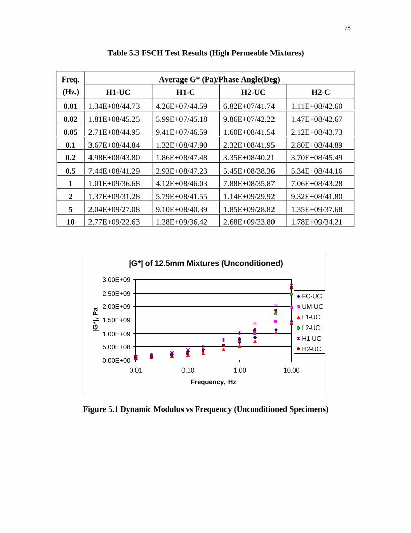
78

Table 5.3 FSCH Test Results (High Permeable Mixtures)

Average G* (Pa)/Phase Angle(Deg)Freq.(Hz.) H1-UC H1-C H2-UC H2-C

0.01 1.34E+08/44.73 4.26E+07/44.59 6.82E+07/41.74 1.11E+08/42.60

0.02 1.81E+08/45.25 5.99E+07/45.18 9.86E+07/42.22 1.47E+08/42.67

0.05 2.71E+08/44.95 9.41E+07/46.59 1.60E+08/41.54 2.12E+08/43.73

0.1 3.67E+08/44.84 1.32E+08/47.90 2.32E+08/41.95 2.80E+08/44.89

0.2 4.98E+08/43.80 1.86E+08/47.48 3.35E+08/40.21 3.70E+08/45.49

0.5 7.44E+08/41.29 2.93E+08/47.23 5.45E+08/38.36 5.34E+08/44.16

1 1.01E+09/36.68 4.12E+08/46.03 7.88E+08/35.87 7.06E+08/43.28

2 1.37E+09/31.28 5.79E+08/41.55 1.14E+09/29.92 9.32E+08/41.80

5 2.04E+09/27.08 9.10E+08/40.39 1.85E+09/28.82 1.35E+09/37.68

10 2.77E+09/22.63 1.28E+09/36.42 2.68E+09/23.80 1.78E+09/34.21

|G*| of 12.5mm Mixtures (Unconditioned)

0.00E+00

5.00E+08

1.00E+09

1.50E+09

2.00E+09

2.50E+09

3.00E+09

0.01 0.10 1.00 10.00

Frequency, Hz

|G*|

, P

a

FC-UC

UM-UC

L1-UC

L2-UC

H1-UC

H2-UC

Figure 5.1 Dynamic Modulus vs Frequency (Unconditioned Specimens)

79

FSCH Tests: 12.5mm Mixtures-Conditioned

0.00E+00

5.00E+08

1.00E+09

1.50E+09

2.00E+09

2.50E+09

3.00E+09

0.01 0.1 1 10

Frequency, Hz

|G*|

, P

aFC-C

UM-UC

H1-C

L1-C

H2-C

L2-C

Figure 5.2 Dynamic Modulus vs Frequency (Conditioned Specimens)

Phase Angles of 12.5mm Mixtures (Unconditioned)

0.00

10.00

20.00

30.00

40.00

50.00

0.01 0.10 1.00 10.00

Frequency,Hz

Ph

ase

An

gle

FC-UC

UM-UC

L1-UC

L2-UC

H1-UC

H2-UC

Figure 5.3 Phase Angle vs Frequency (Unconditioned Specimens)

80

Phase Angles of 12.5mm Mixtures (Conditioned )

0.00

10.00

20.00

30.00

40.00

50.00

0.01 0.10 1.00 10.00

Frequency, Hz

Ph

ase

An

gle

FC-C

UM-C

L1-C

L2-C

H1-C

H2-C

Figure 5.4 Phase Angle vs Frequency (Conditioned Specimens)

For the unconditioned mixtures, the results indicate that three mixtures H1, H2 and L2

have higher stiffness than the other mixtures. The mixture L1 and field specimens have

lower stiffness than the other mixtures. The field cores have lower stiffness than the SGC

specimens. The variability between the stiffness values of H1 and H2 is smaller than

compared to the variability between that of L1 and L2. The stiffness of L1 is at least 45%

of the stiffness of L2. The difference in the stiffness values between the two mixtures of

low permeability indicates that the stiffness of the mixture does not depend on the

permeability of the specimen.

When the specimen is subjected to moisture damage in accordance with AASHTO T-

283, the stiffness of the mixture reduces. The stiffness values of undamaged specimens

are higher than the stiffness values of moisture damaged specimens. After moisture

81

damage, the same set of mixtures H1, H2 and L2 have higher stiffness than the other

mixtures.

The results also show that there is no clear differentiation between the phase angles of

low and high permeability. But the average values of phase angles of high permeable

mixtures are little higher than the phase angles of low permeable mixtures. This trend is

found in both unconditioned and conditioned specimens. Figure 5.5 and Table 5.4

summarize the dynamic modulus of both unconditioned and conditioned specimens. The

percent reduction of stiffness due to moisture induced damage is almost around 50%,

ranging from 33% to 60%. The presence of moisture causes the loss of bonding between

the aggregate surface and the asphalt binder and thereby reduces the stiffness of the

mixture.

Table 5.4 Comparison of |G*| @ 10Hz of 12.5mm Mixtures

|G*| @ 10Hz, PaMixture

Unconditioned Conditioned

% Reduction

FC 1.44E+09 6.21E+08 56.9

UM 1.95E+09 7.75E+08 60.3

L1 1.39E+09 6.35E+08 54.3

L2 2.45E+09 1.36E+09 44.5

H1 2.77E+09 1.28E+09 53.8

H2 2.68E+09 1.78E+09 33.6

82

0.00E+00

5.00E+08

1.00E+09

1.50E+09

2.00E+09

2.50E+09

3.00E+09

FC UM L1 L2 H1 H2

|G*|

at

10 H

z


Figure 5.5 Comparison of Dynamic Modulus at 10 Hz of 12.5mm Mixtures

The fatigue life of a mixture depends on the stiffness of mixture at 10Hz, the

corresponding phase angle and the VFA content. In the SHRP model, the fatigue life of

the mixture is estimated by the combination of these three parameters, (G*| at 10Hz, δ at

10 Hz and VFA. Though the individual values of stiffness and phase angles give unclear

trend with respect to permeability, the estimated fatigue life using these parameters in the

SHRP fatigue model provides a clear trend as discussed in the next chapter.

Statistical Variability:

The average (µ) stiffness values for all the mixtures are summarized in Table 5.5. The

standard deviation (σ) of the stiffness values were calculated. The percentage of σ/µ is a

measure of scatter of data from its average. The results of statistical variability are

summarized in Table 5.5. The results show that the variability in data ranges from 1.6%

83

to 16.1% for unconditioned specimens and from 3.1% to 21.8% for conditioned

specimens.

Table 5.5 Statistical Analysis of |G*| at 10 Hz for 12.5mm Mixtures

Unconditioned ConditionedMixture

µ σ σ/µ*100 µ σ σ/µ*100

FC

UM

L1

L2

H1

H2

1.44E+09

1.95E+09

1.39E+09

2.45E+09

2.77E+09

2.68E+09

1.55E+08

1.25E+08

2.23E+08

4.58E+07

4.36E+07

4.09E+08

10.8

6.4

16.1

1.9

1.6

15.2

6.21E+08

7.75E+08

6.35E+08

1.36E+09

1.28E+09

1.78E+09

1.91E+07

7.49E+07

7.71E+07

2.72E+08

2.79E+08

2.69E+08

3.1

9.7

12.1

20.0

21.8

15.1

Analysis of Variance:

Analysis of Variance (ANOVA) tests were performed on the dynamic modulus values of

12.5mm mixtures. The tests were performed at 95% confidence level. It was

hypothesized that there was no significant difference among the stiffness values of the six

mixtures. The rejection of hypothesis indicates that there exists a statistically significant

difference among the stiffness values of the mixtures. Tables 5.6 and 5.7 furnish the

results of ANOVA tests for unconditioned and conditioned specimens. The Fm statistic

(measured F) and the limiting value of F at certain degrees of freedom is shown in the

tables. The results from the ANOVA table indicate that the Fm statistics are higher than

their limiting values. The Fm values were 18.85 and 16.50 for unconditioned and

conditioned specimens whereas the limiting F value for 95% confidence level is 3.11.

84

This indicates that there exists significant difference among the dynamic modulus values

at 10 Hz of the 12.5mm mixtures.

Table 5.6 ANOVA Results for 12.5mm Mixtures (Unconditioned)

Parameter Sum of

Squares

df Mean Sum

of Squares

Fm F 5,12

Between

treatments

5.61E+18 5 1.12E+18

Error 7.14E+17 12 5.95E+16

Total 6.13E+18 17 3.6E+17

18.85 3.11

Table 5.7 ANOVA Results for 12.5mm Mixtures (Conditioned)

Parameter Sum of

Squares

df Mean Sum

of Squares

Fm F 5,12

Between

treatments

3.33E+18 5 6.66E+17

Error 4.84E+17 12 4.04E+16

Total 3.80E+18 17 2.24E+17

16.50 3.11

5.3.2 FSCH Test Results for 9.5mm Mixtures

The measured dynamic modulus |G*| and phase angle (δ) with respect to loading

frequency from the FSCH test for 9.5mm mixtures are shown in Table 5.8 to 5.10.

Figures 5.6 and 5.7 show the results of stiffness values for all 9.5mm mixtures, both

unconditioned and conditioned specimens. It can be observed that as loading frequency

increases, the stiffness of the mixtures increases. Figures 5.8 and 5.9 show the change of

85

phase angles with varying frequencies for unconditioned as well as conditioned

specimens of all the mixtures.

Table 5.8 Frequency Sweep at Constant Height Test Results(Field Cores and Unmodified)


(Hz.) FC-UC FC-C UM-UC UM-C

0.01 1.17E+08/42.86 7.44E+07/44.59 2.12E+08/38.47 1.21E+08/39.86

0.02 1.55E+08/42.88 9.50E+07/43.95 2.75E+08/38.83 1.57E+08/38.20

0.05 2.13E+08/41.73 1.32E+08/42.10 3.75E+08/37.60 2.13E+08/37.77

0.1 3.15E+08/40.73 2.83E+08/41.96 5.34E+08/37.02 2.99E+08/37.22

0.2 4.42E+08/39.50 3.84E+08/41.75 7.08E+08/35.05 3.95E+08/36.66

0.5 7.26E+08/37.16 5.81E+08/34.43 1.02E+09/31.61 5.84E+08/35.05

1 1.24E+09/33.51 7.73E+08/30.86 1.37E+09/27.33 7.92E+08/30.74

2 1.25E+09/25.15 1.10E+09/26.50 1.62E+09/22.22 1.03E+09/25.57

5 2.37E+09/22.20 1.41E+09/24.89 2.18E+09/19.15 1.44E+09/23.87

10 3.10E+09/19.23 2.23E+09/23.48 2.50E+09/15.34 1.84E+09/19.20

Table 5.9 FSCH Test Results (Low Permeable Mixtures)


(Hz.) L1-UC L1-C L2-UC L2-C

0.01 1.06E+08/37.14 1.47E+08/35.88 2.55E+08/33.67 2.13E+08/39.16

0.02 1.39E+08/37.36 1.82E+08/35.61 3.06E+08/33.40 2.22E+08/38.90

0.05 1.92E+08/36.76 2.36E+08/34.71 3.80E+08/31.71 2.79E+08/35.57

0.1 2.75E+08/36.27 3.20E+08/34.99 5.06E+08/32.08 4.44E+08/35.84

0.2 3.70E+08/35.70 4.14E+08/34.42 6.42E+08/30.31 5.86E+08/36.43

0.5 5.56E+08/34.32 5.83E+08/33.21 9.00E+08/28.92 8.91E+08/34.25

1 7.60E+08/31.82 7.53E+08/30.80 1.17E+09/25.85 1.27E+09/28.89

2 9.21E+08/26.48 9.42E+08/27.76 1.29E+09/22.17 1.35E+09/20.95

5 1.32E+09/24.09 1.22E+09/24.15 1.83E+09/18.05 1.66E+09/18.22

10 1.62E+09/18.73 1.47E+09/20.63 2.16E+09/14.40 1.90E+09/16.52

86

Table 5.10 FSCH Test Results (High Permeable Mixtures)


(Hz.) H1-UC H1-C H2-UC H2-C

0.01 1.22E+08/36.91 1.45E+08/38.03 1.24E+08/38.08 9.38E+07/40.70

0.02 1.65E+08/36.62 1.81E+08/38.36 1.59E+08/37.73 1.19E+08/40.71

0.05 3.04E+08/36.31 2.36E+08/37.03 2.14E+08/36.97 1.56E+08/40.19

0.1 3.75E+08/36.78 3.26E+08/37.46 3.08E+08/36.08 2.19E+08/40.15

0.2 4.96E+08/35.80 4.31E+08/36.88 4.07E+08/35.23 2.89E+08/39.40

0.5 6.80E+08/32.62 6.37E+08/34.83 6.26E+08/33.57 4.22E+08/37.35

1 9.34E+08/28.43 8.60E+08/32.01 8.42E+08/30.88 5.67E+08/35.17

2 1.11E+09/24.42 1.02E+09/28.50 9.97E+08/26.81 7.27E+08/32.63

5 1.83E+09/22.85 1.51E+09/26.98 1.38E+09/23.89 9.92E+08/31.03

10 2.47E+09/19.23 1.87E+09/24.68 1.74E+09/21.11 1.21E+09/28.78

|G*| of 9.5mm Mixtures (Unconditioned)

0.00E+00

5.00E+08

1.00E+09

1.50E+09

2.00E+09

2.50E+09

3.00E+09

3.50E+09

0.01 0.1 1 10

Frequency, Hz

|G*|

@ 1

0 H

z, P

a FC-UC

UM-UC

H1-UC

L1-UC

H2-UC

L2-UC

Figure 5.6 Dynamic Modulus vs Frequency (Unconditioned Specimens)

87

|G*| of 9.5mm Mixtures (Conditioned)

0.00E+00

5.00E+08

1.00E+09

1.50E+09

2.00E+09

2.50E+09

3.00E+09

3.50E+09

0.01 0.1 1 10

Frequency, Hz

|G*|

@ 1

0 H

z, P

a FC-C

UM-UC

H1-C

L1-C

H2-C

L2-C

Figure 5.7 Dynamic Modulus vs Frequency (Conditioned Specimens)

Phase Angles of 9.5mm Mixtures (Unconditioned)

0

10

20

30

40

50

0.01 0.1 1 10Frequency, Hz

Ph

ase

An

gle

FC-UC

UM-UC

H1-UC

L1-UC

H2-UC

L2-UC

Figure 5.8 Phase Angle vs Frequency (Unconditioned Specimens)

88

Phase Angles of 9.5mm Mixtures (Conditioned)

0

10

20

30

40

50

0.01 0.1 1 10

Frequency, Hz

Ph

ase

An

gle

FC-C

UM-UC

H1-C

L1-C

H2-C

L2-C

Figure 5.9 Phase Angle vs Frequency (Conditioned Specimens)

Figure 5.10 and Table 5.11 summarize the dynamic modulus of both unconditioned and

conditioned specimens. The results show that the field cores have higher stiffness than

the other mixtures. The mixtures L1 and H2 have lower stiffness than the mixtures L2

and H1. The mixtures H1 and UM have almost same stiffness values for unconditioned

specimens. This trend is found in both unconditioned and conditioned specimens. Even

though there is no clear trend observed in the phase angles of the mixtures but the phase

angles of high permeable mixtures are little higher than the phase angles of low

permeable mixtures. A reduction in the stiffness of mixtures is observed after the

conditioning of mixtures. The conditioned specimens have higher phase angles than the

unconditioned specimens. The mixtures with low permeability have lower reduction in

stiffness around 10% compared to other mixtures. The other mixtures have reduced

stiffness of around 25% due to moisture damage. The water induced during the

conditioning process causes the damage in the form of stripping of aggregate surfaces

and asphalt binder and hence the reduction in stiffness.

89

Table 5.11 Comparison of |G*| @ 10Hz of 9.5mm Mixtures

|G*| @ 10Hz, PaMixture


% Reduction

FC 3.10E+09 2.23E+09 28.1

UM 2.50E+09 1.84E+09 26.4

L1 1.62E+09 1.47E+09 9.3

L2 2.16E+09 1.90E+09 12.0

H1 2.47E+09 1.87E+09 24.3

H2 1.74E+09 1.21E+09 30.5

0.00E+00

1.00E+09

2.00E+09

3.00E+09

4.00E+09

FC UM L1 L2 H1 H2

|G*|

@10

Hz


Figure 5.10 Comparison of Dynamic Modulus at 10 Hz of 9.5mm Mixtures

90


The average (µ) stiffness values for all the 9.5mm mixtures are summarized in Table

5.12. The standard deviation (σ) of the stiffness values were also calculated. The

percentage of σ/µ is a measure for determining the variability in the data. The results of

statistical variability are summarized in Table 5.12. The results show that the variability

in data ranges from around 10% to 20% for unconditioned specimens and from 5.5% to

18.1% for conditioned specimens.


Analysis of Variance (ANOVA) tests were also performed on the dynamic modulus

values of 9.5mm mixtures. The tests were performed at the same 95% confidence level. It

was hypothesized that there was no significant difference among the stiffness values of

all the mixtures. The rejection of hypothesis indicates that there exists a statistically

significant difference among the stiffness values of the mixtures. Tables 5.13 and 5.14

furnish the results of ANOVA tests for unconditioned and conditioned specimens. The Fm

statistics and the limiting value of F at certain degrees of freedom are shown in the tables.

The ANOVA results indicate that the Fm statistics are higher than their limiting values.

The Fm values were 17.16 and 5.47 for unconditioned and conditioned specimens

whereas the limiting F value for 95% confidence level is 3.11. Thus there exists a

significant difference among the dynamic modulus values at 10 Hz of the 9.5mm

mixtures.

91

Table 5.12 Statistical Analysis of |G*| at 10 Hz for 12.5mm Mixtures


µ σ σ/µ*100 µ σ σ/µ*100

FC

UM

L1

L2

H1

H2

3.10E+09

2.50E+09

1.62E+09

2.16E+09

2.47E+09

1.74E+09

3.06E+08

4.94E+08

3.16E+08

3.82E+08

4.10E+08

2.80E+08

9.9

19.7

19.5

17.7

14.2

16.1

2.23E+09

1.84E+09

1.47E+09

1.90E+09

1.87E+09

1.21E+09

2.63E+08

1.18E+08

8.08E+07

3.08E+08

3.39E+08

1.18E+08

11.8

6.4

5.5

16.2

18.1

9.8


Parameter Sum of

Squares

df Mean Sum

of Squares

Fm F 5,12

Between

treatments

5.46E+18 5 1.09E+18

Error 7.64E+17 12 6.37E+16

Total 7.12E+18 17 4.19E+17

17.16 3.11


Parameter Sum of

Squares

df Mean Sum

of Squares

Fm F 5,12

Between

treatments

1.92E+18 5 3.84E+17

Error 8.43E+17 12 7.02E+16

Total 2.55E+18 17 1.50E+17

5.47 3.11

92

5.4 Repeated Shear Test at Constant Height

This test was performed to measure the accumulating plastic shear strain of the mixtures

and there by estimating their rutting potential. The visco-elastic properties of an asphalt

mixture at high temperatures are related to its permanent deformation characteristics. The

accumulation of plastic shear strain in a mixture under repeated loading can give some

indication about the mixture’s resistance to permanent deformation. The repeated shear

testing at constant height was selected to evaluate the accumulated shear strain and

permanent deformation characteristics of the mixtures.

The RSCH test is a stress-controlled test with the feedback to the vertical load actuator

from the magnitude of the shear load. The test is conducted at constant height, requiring

the vertical actuator to be controlled by the vertical LVDT. The horizontal actuator under

control by the shear load cell applies haversine loads. It preconditions the specimen by

applying a haversine load corresponding to a 7-kPa shear stress for 100 cycles. The 0.7-

second load cycle consists of a 0.1-second shear load followed by 0.6-second rest period.

After preconditioning the specimen, it applies a 68 ± 5 kPa haversine shear pulse for

5,000 cycles or until 5% shear strain is reached. This corresponds to a frequency of

approximately 1.43 Hz. During the test, axial and shear loads and deformations are

measured and recorded. This test was conducted according to AASHTO TP-7 Procedure

F (15). RSCH tests were performed on specimens of four mixtures and three compaction

methods. The tests were conducted at their respective seven-day average high pavement

temperature at 50-mm depth from the pavement surface.

93

5.5 Analysis of RSCH Test Results

Three replicate specimens were used to conduct the RSCH test. Since the FSCH test is a

nondestructive test, the replicates were reused for the destructive RSCH test. All mixtures

were tested using the RSCH test at a temperature of 58.4oC. The RSCH tests were

conducted either for 5000 loading cycles or until the maximum shear strain of 5% was

reached, whichever was earlier. The permanent shear strain accumulated at the end of

5000 cycles was measured. This shear strain was used for predicting the in-service rut

depth using the SHRP Rutting model, as discussed in the next chapter. The results of

RSCH tests for both 12.5mm and 9.5mm mixtures are discussed in the following

sections.

5.5.1 RSCH Test Results for 12.5mm Mixtures

Table 5.15 furnishes the results of RSCH test results for 12.5mm mixtures. The shear

strains for both unconditioned specimens and conditioned specimens are provided. In

Figures 5.11 and 5.12, the change of plastic shear strain with number of loading cycles is

plotted for unconditioned and conditioned specimens, respectively. Figure 5.13 shows a

bar chart comparing the shear strains of all the mixtures.

All the mixtures passed the RSCH test criterion of 5000 cycles. This indicates that the

designed mixtures have good resistance for rutting and are expected have rut depths

below the allowable rut depth of 0.5 inch. The results show that the shear strains of

mixtures of high permeability of unconditioned specimens are higher than the other

mixtures. The mixtures of low permeability have lower shear strains than the field cores

94

and the mixture of unmodified gradation. The results of conditioned specimens show that

mixtures of high permeability have higher shear strains. The field cores and the mixture

of unmodified gradation have lower shear strains. The mixture L1 has much higher shear

strain in conditioned state than in unconditioned state. The shear strains of unconditioned

specimens are higher than the shear strains of the conditioned specimens. The increase in

shear strain indicates the loss in shear strength of the mixtures due to the damage induced

during the conditioning. The increase in shear strain due to conditioning is higher in the

mixtures of low permeability than in the mixtures of high permeability. This observation

was drawn out from the results of the RSCH tests. The low permeable mixtures have

higher moisture damage than high permeable mixtures owing to higher surface area

available for stripping. However, low permeable pavement sections may not experience

more rutting damage than the high permeable pavement sections.

The moisture damage in specimens is induced in the laboratory in accordance with the

AASHTO T-283 procedure. The specimens are saturated to a level of 70% and then

conditioned for 24 hours at 60oC. The low permeable mixtures would generally take

longer time than the high permeable mixtures to reach any level of saturation.

Irrespective of the permeability levels, the specimens are forced to saturate to the same

level for both low and high permeable mixtures. In the field, the pavement sections take

their natural course of time to saturate to a given level due to the different levels of

permeability. The low permeable pavement sections would take longer time than the high

permeable pavement sections to reach the same level of saturation that would activate the

moisture related damage.

95

Table 5.15 RSCH Test Results of 12.5mm Mixtures


Shear Strain Cycles Shear Strain Cycles

Field Cores

Unmodified

Low Perm – 1

Low Perm – 2

High Perm – 1

High Perm - 2

0.0207

0.0220

0.0132

0.0154

0.0310

0.0320

5000

5000

5000

5000

5000

5000

0.0308

0.0270

0.0368

0.0292

0.0339

0.0381

5000

5000

5000

5000

5000

5000

12.5mm Mixtures - Unconditioned

0

0.005

0.01

0.015

0.02

0.025

0.03

0.035

0 1000 2000 3000 4000 5000 6000

Number of Cycles

Pla

stic

Sh

ear

Str

ain

FC

UM

L1

L2

H1

H2

Figure 5.11 RSCH Test Results for 12.5mm Mixtures (Unconditioned)

96

12.5mm Mixtures - Conditioned

0.000

0.005

0.010

0.015

0.020

0.025

0.030

0.035

0.040

0 1000 2000 3000 4000 5000 6000

Number of Cycles

Pla

stic

Sh

ear

Str

ain

FCD

UMD

L1D

L2D

H1D

H2D

Figure 5.12 RSCH Test Results for 12.5mm Mixtures (Conditioned)

0

0.01

0.02

0.03

0.04

FC UM L1 L2 H1 H2

Sh

ear

Str

ain


Figure 5.13 Comparison of Shear Strains of 12.5mm Mixtures


The average (µ) shear strains for all the 12.5mm mixtures are summarized in Table 5.16.

The standard deviation (σ) of the stiffness values were also calculated. The percentage of

σ/µ is a measure of scatter of data from its average. The results of statistical variability

97

are summarized in Table 5.16. The results show that the variability in data is around 10%

for unconditioned specimens as well as conditioned specimens.


Analysis of Variance (ANOVA) tests were also performed on the shear strains of

12.5mm mixtures. The tests were performed at the same 95% confidence level. It was

hypothesized that there was no significant difference among the shear strains of the



results of ANOVA tests for unconditioned and conditioned specimens. The Fm statistics

and the limiting value of F at certain degrees of freedom are shown in the tables. The

ANOVA results indicate that the Fm statistics are higher than their limiting values. The

Fm values were 18.88 and 6.16 for unconditioned and conditioned specimens whereas the

limiting F value for 95% confidence level is 3.11. Thus there exists a significant

difference among the shear strains of the 12.5mm mixtures. The Fm value of conditioned

specimens is lower than that of unconditioned specimens. The above observation

indicates that the magnitude of difference in shear strains among the mixtures in

unconditioned state decreases compared to the shear strains of the same specimens

measured after conditioning. The decrease in Fm is due to the fact that the effect of

moisture damage on shear strains of low permeable mixtures is higher than that of high

permeable mixtures.

98

Table 5.16 Statistical Analysis of Shear Strain for 12.5mm Mixtures


µ σ µ/σ*100 µ σ µ/σ*100

FC

UM

L1

L2

H1

H2

0.021

0.022

0.0132

0.0154

0.031

0.032

2.43E-03

1.74E-03

1.01E-03

1.14E-03

2.32E-03

3.84E-03

11.6

7.9

7.7

7.4

7.6

12.0

0.0308

0.0270

0.0368

0.0292

0.0339

0.038

1.93E-03

1.47E-03

3.16E-03

6.81E-04

3.61E-04

3.61E-03

6.3

5.5

8.5

2.3

1.1

9.6


Parameter Sum of

Squares

df Mean Sum

of Squares

Fm F 5,12

Between treatments 8.87E-04 5 1.77E-04

Error 1.13E-04 12 9.40E-06

Total 9.50E-04 17 5.59E-05

18.88 3.11


Parameter Sum of

Squares

df Mean Sum

of Squares

Fm F 5,12

Between treatments 2.78E-04 5 5.55E-04

Error 1.08E-04 12 9.01E-06

Total 3.37E-04 17 1.98E-05

6.16 3.11

99

5.5.2 RSCH Test Results for 9.5mm Mixtures

Table 5.19 provides the shear strains of 9.5mm mixtures in unconditioned as well as

conditioned states. In Figures 5.14 and 5.15, the change of plastic shear strain with

number of loading cycles is plotted for unconditioned and conditioned specimens,

respectively. A comparison of shear strains is shown in Figure 5.16.

The results of 9.5mm mixture indicate that the shear strains of mixtures with high

permeability of unconditioned specimens are higher than the other mixtures. The

mixtures of low permeability have lower shear strains than the field cores and the mixture

of unmodified gradation. The results of conditioned specimens show that mixtures of

high permeability have higher shear strains than other mixtures. The mixtures L1 and L2

have lower shear strains than other mixtures in conditioned state too. The field cores and

the mixture of unmodified gradation have shear strains in between low permeable and

high permeable mixtures.

The shear strains of conditioned specimens are higher than the shear strains of the

unconditioned specimens. The increase in shear strain indicates the loss in shear strength

of the mixtures due to the damage induced during the conditioning. The increase in shear

strain due to conditioning is higher in the mixtures of low permeability than in the

mixtures of high permeability. In spite of a greater increase in shear strain as observed in

low permeable mixtures due to conditioning, the shear strains of mixtures L1 and L2 are

lower than the mixtures H1 and H2.

100

Table 5.19 RSCH Test Results of 9.5mm Mixtures


Shear Strain Cycles Shear Strain Cycles

Field Cores

Unmodified

Low Perm 1

Low Perm 2

High Perm 1

High Perm 2

0.0200

0.0211

0.0164

0.0126

0.0256

0.0241

5000

5000

5000

5000

5000

5000

0.0366

0.0277

0.0225

0.0211

0.0332

0.0308

5000

5000

5000

5000

5000

5000

9.5mm Mixtures- Unconditioned

0

0.005

0.01

0.015

0.02

0.025

0.03

0 1000 2000 3000 4000 5000 6000

Number of Cycles

Pla

stic

Sh

ear

Str

ain

FC

UM

L1

L2

H1

H2

Figure 5.14 RSCH Test Results for 9.5mm Mixtures (Unconditioned)

101

9.5mm Mixtures - Conditioned

00.0050.01

0.0150.02

0.0250.03

0.0350.04

0 1000 2000 3000 4000 5000 6000

Number of Cycles

Pla

stic

Sh

ear

Str

ain FCD

UMD

L1D

L2D

H1D

H2D

Figure 5.15 RSCH Test Results for 9.5mm Mixtures (Conditioned)

0

0.01

0.02

0.03

0.04

FC UM L1 L2 H1 H2

Sh

ear

Str

ain


Figure 5.16 Comparison of Shear Strains of 9.5mm Mixtures


The average (µ) shear strains for all the 12.5mm mixtures are summarized in Table 5.20.

The standard deviation (σ) of the stiffness values were also calculated. The percentage of

σ/µ gives is a measure to explain the scatter of data. The results of statistical variability

102

are summarized in Table 5.20. The results show that the variability in data ranges from

3.7% to 14% for unconditioned specimens and from 4.2% to 19.5% for conditioned

specimens.


Analysis of Variance (ANOVA) tests were also performed on the shear strains of 9.5 mm

mixtures. The tests were performed at the same 95% confidence level. It was

hypothesized that there was no significant difference among the shear strains of the



results of ANOVA tests for unconditioned and conditioned specimens. The Fm statistics

and the limiting value of F at certain degrees of freedom are shown in the tables. The

ANOVA results indicate that the Fm statistics are higher than their limiting values. The

Fm values were 15.0 and 7.2 for unconditioned and conditioned specimens whereas the

limiting F value for 95% confidence level is 3.11. Thus there exists a significant

difference among the shear strains of the 12.5mm mixtures. As observed in the 12.5mm

mixtures, the difference in Fm between unconditioned and conditioned mixtures can be

attributed to the fact that the percent increase in shear strains of high permeable mixtures

due to moisture damage is lower than the percent increase in shear strains of low

permeable mixtures.

103

Table 5.20 Statistical Analysis of Shear Strain for 9.5mm Mixtures


µ σ µ/σ*100 µ σ µ/σ*100

FC

UM

L1

L2

H1

H2

0.0200

0.0211

0.0164

0.0126

0.0256

0.0241

1.53E-03

1.60E-03

6.08E-04

1.70E-03

3.61E-03

1.97E-03

7.8

7.6

3.7

13.5

14.1

8.2

0.0366

0.0277

0.0225

0.0211

0.0332

0.0308

7.11E-03

3.05E-03

9.50E-04

8.72E-04

4.19E-03

3.75E-03

19.5

11.0

4.2

4.2

12.6

12.2


Parameter Sum of

Squares

df Mean Sum

of Squares

Fm F 5,12

Between

treatments

3.51E-04 5 7.02E-04

Error 5.62E-04 12 4.68E-06

Total 4.01E-04 17 2.36E-05

15.00 3.11


Parameter Sum of

Squares

df Mean Sum

of Squares

Fm F 5,12

Between

treatments

5.59E-04 5 1.12E-04

Error 1.86E-04 12 1.55E-05

Total 7.45E-04 17 4.39E-05

7.20 3.11

104

5.6 APA Rut Tests

The APA rut tests were conducted on specimens of both 12.5mm and 9.5mm mixtures to

evaluate the rutting susceptibility of the mixtures. The Asphalt Pavement Analyzer

(APA) is a modification of the Georgia Loaded Wheel Tester (GLWT) and was first

manufactured in 1996 by Pavement Technology, Inc. The APA is a multifunctional

Loaded Wheel Tester used for evaluating permanent deformation, fatigue cracking and

moisture susceptibility. The APA features controllable wheel load and contact pressure

that are representative of actual field conditions. Each sample is subjected to repetitive

linear wheel tracking actions with controlled pressure on cylindrical or beam specimens

for rut testing. The theory behind a loaded wheel tester is to apply an appropriate cyclical

loading to asphalt concrete specimens to best simulate actual traffic. This is accomplished

by air pressurized hoses lying across samples with a loaded wheel coming in contact with

the hose and applying a predetermined load to the hose and thus the specimens. The

wheel rolls back and forth up to 8,000 times or cycles. The rut depth is then measured at

the end of 8000 loading cycles.

In the APA testing, only rutting potential of the mixtures was investigated. The rutting

tests were conducted on the field cores and unconditioned specimens of all the mixtures.

All the specimens were tested at 8.5% air voids. The test temperature was 64oC. The

results of the APA test on unconditioned specimens are given in Table 5.23. The rut

depths are compared in Figure 5.17. There are few issues in the evaluation of conditioned

specimens using the APA rut test. As a simulative test, the mechanism of rutting in APA

rut test is different from the measurement of shear strain in RSCH test. Only two of the

105

six mixtures were tested for rutting in the conditioned state. The results of APA test of

mixtures after conditioning are provided in Table 5.24.

Table 5.23 APA Rut Depths of Unconditioned Specimens

APA Rut Depth, mm


Field Cores 4.78 4.11

Unmodified 4.98 4.27

Low Perm 1 4.47 3.90

Low Perm 2 4.55 3.22

High Perm 1 5.75 5.26

High Perm 2 5.41 4.48

Table 5.24 APA Rut Depth of Conditioned Specimens


Low Perm 2 4.62 2.13

High Perm 2 5.03 3.64

APA Rut Depths

0

1

2

3

4

5

6

7

12.5mm 9.5mmMixtures

Ru

t D

epth

, mm

FC

UM

L1

L2

H1

H2

Figure 5.17 Comparison of APA Rut Depths of Unconditioned Mixtures

106

As indicated by the results in Table 5.23, the trends of APA rut tests reasonably agree

with shear strain trends of RSCH tests. The low permeable mixtures have lower rut

depths than high permeable mixtures and unmodified mixtures. The high permeable

mixtures have higher rut depths than all other mixtures. The same trend was observed in

the results of RSCH tests. For conditioned mixtures, the APA rut depths of low

permeable mixtures (12.5 L2 and 9.5 L2) were a little lower than the rut depths of high

permeable mixtures (12.5 H2 and 9.5 H2).

However, the rut depths of conditioned specimens are lower than the rut depths of

unconditioned specimens. The decrease in rut depth of mixtures due to conditioning is

contrary to the expected trends. The conditioning procedure of the specimens might have

contributed to this unexpected trend. The APA test was conducted on conditioned

specimens in dry state. The ASTM procedure recommends slightly a different method for

determining moisture susceptibility of mixtures by the APA test using freeze-thaw cycles.

In this study, dry specimens after AASHTO T-283 conditioning were used for the APA

test, as the same procedure was adopted for the RSCH test. But the AASHTO T-283

procedure was not successful in measuring the effect of moisture damage on APA rut

depths.

The stiffness, phase angles and shear strains of mixtures were used for performance

prediction of mixtures in the estimation of fatigue and rutting life. The performance of

low and high permeable mixtures and the effects of moisture damage are discussed in the

Chapter 6.

107

CHAPTER 6

PERFORMANCE ANALYSIS OF MIXTURES

The FSCH tests and RSCH tests were conducted to characterize the material properties of

12.5mm and 9.5mm mixtures. The stiffness, phase angle and shear strain of the mixtures

are the material responses that were used to predict the pavement’s performance under

service for distresses such as fatigue cracking and rutting. Fatigue and Rutting analysis

are performed using surrogate models developed by SHRP 003-A project. Fatigue

analysis of SHRP model considers material properties as well as pavement structural

layer thickness whereas rutting analysis considers only the material properties.

6.1 SUPERPAVE Fatigue Model Analysis

The abridged fatigue analysis system from SHRP A-003A predicts the resistance of mix

to fatigue distress for a pavement structure under a given traffic load. The resistance of a

mix to fatigue cracking depends on the material properties such as initial flexural loss

stiffness and voids filled with asphalt (VFA) and the pavement structural property,

horizontal tensile strain at the bottom of the asphalt concrete layer. The abridged

procedure requires an estimate of the flexural stiffness modulus of the asphalt aggregate

mix at 20oC (19). The flexural stiffness can be estimated from the shear stiffness of the

mixture as measured from the FSCH tests at 10 Hz at 20oC. This estimate is used in the

multilayer elastic analysis to determine the critical level of strain to which the mix is

subjected under the standard traffic load.

108

Multi-layer elastic analysis is used to determine the design strain, the maximum principal

tensile strain at the bottom of the asphalt concrete layer, under the standard AASHTO

axle load of 18 kips. For this purpose, a pavement structure was assumed to conduct this

analysis. The pavement structure and loading are given in Figure 6.1. The assumed

pavement structure consists of an asphalt concrete layer, an aggregate base course, a

subbase resting on the subgrade. The asphalt concrete layer is 4 inches thick and the two

layers beneath have a thickness of 8 inches each. The Poisson ratios and modulus of

layers are shown in Figure 6.1. A standard 18-kip single axle load with dual tires inflated

to 100 psi was used. The horizontal tensile strains at the bottom of AC layer are estimated

at outer edge, center, inner edge, and center of dual tires using EVERSTRESS software for

multilayer elastic analysis of pavement sections. The critical tensile strain is used as the

design strain in this analysis.

The flexural properties of the mixtures are estimated using the following regression

equations.

So = 8.56 * (Go)0.913 R2 = 0.712

So” = 81.125 * (Go”)0.725 R2 = 0.512

where

So = initial flexural stiffness at 50th loading cycle is psi

Go = shear stiffness at 10 Hz in psi

So” = initial flexural loss stiffness at 50th loading cycle is psi

Go” = shear loss stiffness at 10 Hz in psi

109

Figure 6.1 Typical Pavement Structure and Loading

The fatigue resistance of a mix is then estimated from the following strain-dependent

surrogate model.

Nsupply = 2.738E5* e 0.077VFB* ε0-3.624* S0” –2.72

where

Nsupply = estimated fatigue life of the given pavement section in ESALs

VFB = voids filled with asphalt

ε0 = critical tensile strain at the bottom of AC layer

AC Layer E from FSTCH 4" thick ν =0.35

Agg. Base Course E = 35 ksi 8" thick ν = 0.35

Subbase E = 20 ksi 8" thick ν = 0.40

Subgrade E = 5 ksi ν = 0.45

4500 lb 4500 lbSingle AxleDual tires 12" c/cTire Pressure 100 psiContact radius 3.78"

110

The coefficient of determination for the surrogate model for fatigue analysis is 0.79 with

a coefficient of variation of 90 percent. The estimation of fatigue life for 12.5mm

mixtures and 9.5mm mixtures are discussed in the following sections.

6.1.1 Fatigue Analysis of 12.5mm Mixtures

The fatigue life of the 12.5mm mixtures were estimated using the abridged fatigue

analysis system for both unconditioned and conditioned specimens. First, the flexural

stiffness modulus values of the mixtures were estimated using the shear stiffness and

phase angles at 10 Hz measured in the FSCH tests. The flexural and shear modulus

values of 12.5mm mixtures are summarized in Table 6.1.

Table 6.1 Summary of Estimated Material Properties for 12.5mm Mixtures

Mix |G*| pa PhaseAngle

|G*| psi Go'' So So''

FC-UC 1.44E+09 17.5 2.09E+05 6.29E+04 6.16E+05 2.44E+05

FC-C 6.21E+08 29.8 9.01E+04 4.48E+04 2.86E+05 1.91E+05

UM-UC 1.95E+09 20.9 2.83E+05 1.01E+05 8.12E+05 3.45E+05

UM-C 7.75E+08 34.8 1.12E+05 6.42E+04 3.50E+05 2.48E+05

L1-UC 1.39E+09 22.9 2.02E+05 7.83E+04 5.96E+05 2.87E+05

L1-C 6.35E+08 38.1 9.21E+04 5.68E+04 2.92E+05 2.27E+05

L2-UC 2.45E+09 21.6 3.55E+05 1.31E+05 1.00E+06 4.15E+05

L2-C 1.36E+09 28.9 1.97E+05 9.52E+04 5.85E+05 3.30E+05

H1-UC 2.77E+09 22.6 4.02E+05 1.54E+05 1.12E+06 4.69E+05

H1-C 1.28E+09 36.4 1.86E+05 1.10E+05 5.53E+05 3.67E+05

H2-UC 2.68E+09 23.8 3.89E+05 1.57E+05 1.09E+06 4.74E+05

H2-C 1.78E+09 34.2 2.58E+05 1.45E+05 7.47E+05 4.48E+05

111

The fatigue resistance of the mixtures, as expected in service life of the pavement, is

estimated in terms of number of ESALs (Nsupply) that corresponds to 50% reduction in

the mixture stiffness. The Nsupply values were estimated by considering the flexural loss

modulus, voids filled with asphalt (VFA) and critical tensile strain at the bottom of

asphalt concrete layer, as shown in Table 6.2. The results for 12.5mm mixtures are

summarized in Table 6.3 and Figure 6.2. The percent reduction in fatigue life of different

mixtures due to conditioning is given in Table 6.3.

Table 6.2 Fatigue Life Analysis of 12.5mm Mixtures

Mix So" VFA Strain Nsupply

FC-UC 2.44E+05 71.92 2.37E-04 2.11E+06

FC-C 1.91E+05 71.92 3.29E-04 1.25E+06

UM-UC 3.45E+05 71.92 2.06E-04 1.37E+06

UM-C 2.48E+05 71.92 3.05E-04 8.15E+05

L1-UC 2.87E+05 75.8 2.41E-04 1.74E+06

L1-C 2.27E+05 75.8 3.27E-04 1.09E+06

L2-UC 4.15E+05 74.35 1.85E-04 1.48E+06

L2-C 3.30E+05 74.35 2.43E-04 1.02E+06

H1-UC 4.69E+05 74.67 1.74E-04 1.37E+06

H1-C 3.67E+05 74.67 2.50E-04 7.15E+05

H2-UC 4.74E+05 74.8 1.76E-04 1.28E+06

H2-C 4.48E+05 74.8 2.16E-04 7.13E+05

112

Table 6.3 Summary of Fatigue Life of 12.5mm Mixtures (Nsupply)

Mix Unconditioned

(UC)

Conditioned

(C)

Percent Difference

= (UC- C)/UC *100

Field Cores

Unmodified

Low Perm – 1

Low Perm – 2

High Perm – 1

High Perm - 2

2.11E+06

1.37E+06

1.74E+06

1.48E+06

1.37E+06

1.28E+06

1.25E+06

8.15E+05

1.09E+06

1.02E+06

7.15E+05

7.13E+05

40.5

40.3

37.4

31.1

48.0

44.4

Fatigue Life of 12.5mm Mixtures

0.00E+00

5.00E+05

1.00E+06

1.50E+06

2.00E+06

2.50E+06

FC U L1 L2 H1 H2

Nsu

pp

ly E

SA

Ls

UC

C

Figure 6.2 Fatigue Life of 12.5mm Mixtures

The results clearly indicate that the mixtures of low permeability have higher fatigue life

than the mixtures of higher permeability in both states of conditioning. For the

unconditioned specimens, the field cores have the highest fatigue life. The SGC

compacted specimen that had the same gradation as that of the field cores have lower

fatigue life than the field cores. The same trend is observed even after conditioning.

113

These specimens experience the same amount of reduction in fatigue life due to the

damage caused during the conditioning process. The low permeable mixtures have higher

fatigue life than the high permeable mixtures and the mixture of unmodified gradation.

The mixture L1 has better fatigue life than L2 for the low permeable mixtures whereas

the mixture H1 is better than H2 for the high permeable mixtures. This trend is observed

in both states of conditioning.

The fatigue life values of low permeable mixtures, L1 and L2, reduce by 37.4 % and 31.1

% due to moisture damage, respectively. The high permeable mixtures, H1 and H2 have a

reduction of 48.0% and 44.4% in their fatigue life due to moisture damage, respectively.

For field cores and the unmodified mixtures, the fatigue life reduces by almost 40.5% and

40.3%, respectively. The Nsupply values and the percent reduction due to conditioning

indicate that the mixtures with low permeability have higher fatigue life and lower

damage compared to the mixtures of high permeability. The loss in tensile strength could

be lower in low permeable mixtures than in the high permeable mixtures.


The ANOVA tests were conducted for the results of fatigue life of 12.5mm mixtures. The

values of fatigue life given in Table 6.2 were calculated by assuming the mean dynamic

modulus and phase angle at 10Hz of each mixture. The values used in Table 6.1 and 6.2

are the mean averages of data points of three replicates used in FSCH tests. The

individual data points, |G*| and δ at 10 Hz, were used to compute the individual fatigue

life values of mixtures for the ANOVA test. The test was conducted to check whether at

114

least one significant difference exists among the fatigue life values of mixtures. The

ANOVA tests were conducted separately for unconditioned and conditioned mixtures.

The results of the ANOVA tests are provided in Tables 6.4 and 6.5 for unconditioned and

conditioned mixtures, respectively.

Table 6.4 ANOVA Results for Fatigue Life of 12.5mm Mixtures (Unconditioned)

Parameter Sum of

Squares

df Mean Sum

of Squares

F* F 5,12

Between treatments 1.51E+12 5 3.01E+11

Error 3.91E+11 12 3.26E+10

Total 1.90E+12 17 1.12E+11

9.24 3.11

Table 6.5 ANOVA Results for Fatigue Life of 12.5mm Mixtures (Conditioned)

Parameter Sum of

Squares

df Mean Sum

of Squares

F* F 5,12

Between

treatments

6.29E+11 5 1.28E+11

Error 8.35E+10 12 6.96E+09

Total 7.23E+11 17 4.25E+10

18.37 3.11

The results show that the computed F* statistic is greater than the limiting F value at 95%

confidence level for both type of specimens. This indicates that at least one significant

difference exists among the fatigue life values of mixtures. This difference is more

115

pronounced among the conditioned specimens than the unconditioned specimens as the

F* value of conditioned specimens (18.37) is higher than the F* value of unconditioned

specimens (9.24)

6.1.2 Fatigue Analysis of 9.5mm Mixtures

The fatigue life of the 9.5mm mixtures were estimated using the abridged fatigue analysis

system for both unconditioned and conditioned specimens. The estimations of flexural

and shear modulus values of 9.5mm mixtures are summarized in Table 6.6.

Table 6.6 Summary of Estimated Material Properties for 9.5mm Mixtures

Mix |G*| pa Phase |G*| psi Go'' So So''

FC-UC 3.10E+09 19.23 4.50E+05 1.48E+05 1.24E+06 4.55E+05

FC-C 2.23E+09 23.48 3.23E+05 1.29E+05 9.18E+05 4.11E+05

UM-UC 2.50E+09 15.34 3.63E+05 9.59E+04 1.02E+06 3.32E+05

UM-C 1.84E+09 19.20 2.67E+05 8.78E+04 7.70E+05 3.11E+05

L1-UC 1.62E+09 18.73 2.35E+05 7.54E+04 6.86E+05 2.79E+05

L1-C 1.47E+09 20.63 2.13E+05 7.51E+04 6.28E+05 2.78E+05

L2-UC 2.16E+09 14.40 3.13E+05 7.79E+04 8.92E+05 2.85E+05

L2-C 1.90E+09 16.52 2.76E+05 7.84E+04 7.93E+05 2.87E+05

H1-UC 2.47E+09 19.23 3.58E+05 1.18E+05 1.01E+06 3.86E+05

H1-C 1.87E+09 24.68 2.71E+05 1.13E+05 7.82E+05 3.74E+05

H2-UC 1.74E+09 21.11 2.52E+05 9.09E+04 7.32E+05 3.19E+05

H2-C 1.21E+09 28.78 1.75E+05 8.45E+04 5.25E+05 3.03E+05

116

The fatigue life of mixtures was estimated using the SHRP fatigue relationship discussed

earlier in this chapter. The Nsupply values as estimated by considering the flexural loss

modulus, voids filled with asphalt (VFA) and critical tensile strain at the bottom of

asphalt concrete layer are shown in Table 6.7. The results for 9.5mm mixtures are

summarized in Table 6.8 and Figure 6.3. The percent reduction in fatigue life due to

conditioning of different mixtures is given in Table 6.8.

Table 6.7 Fatigue Life Analysis of 9.5mm Mixtures

Mix So" VFA Strain Nsupply

FC-UC 4.55E+05 72.38 1.64E-04 1.54E+06

FC-C 4.11E+05 72.38 1.94E-04 1.11E+06

UM-UC 3.32E+05 72.38 1.83E-04 2.44E+06

UM-C 3.11E+05 72.38 2.12E-04 1.69E+06

L1-UC 2.79E+05 77.2 2.25E-04 2.67E+06

L1-C 2.78E+05 77.2 2.35E-04 2.30E+06

L2-UC 2.85E+05 75.25 1.97E-04 3.53E+06

L2-C 2.87E+05 75.25 2.09E-04 2.79E+06

H1-UC 3.86E+05 73.8 1.84E-04 1.78E+06

H1-C 3.74E+05 73.8 2.11E-04 1.17E+06

H2-UC 3.19E+05 75.83 2.18E-04 1.88E+06

H2-C 3.03E+05 75.83 2.56E-04 1.21E+06

It is evident from the results of 9.5mm mixtures that the mixtures of low permeability

have higher fatigue life than the mixtures of higher permeability in both states of

conditioning. The mixture L2 has the highest fatigue life in unconditioned and

conditioned state. Another low permeable mixture, L1 has the second highest fatigue life

among all the mixtures. The high permeable mixtures have lower fatigue life than the low

117

permeable mixtures and the unmodified mixture. This trend is observed in both states of

conditioning.

Table 6.8 Summary of Fatigue Life of 9.5mm Mixtures (Nsupply)

Mix Unconditioned

(UC)

Conditioned

(C)

Percent Difference

= (UC- C)/UC *100

Field Cores

Unmodified

Low Perm – 1

Low Perm – 2

High Perm – 1

High Perm - 2

1.54E+06

2.44E+06

2.67E+06

3.53E+06

1.78E+06

1.88E+06

1.11E+06

1.69E+06

2.30E+06

2.79E+06

1.17E+06

1.21E+06

27.9

30.6

13.8

20.9

34.0

35.7

Fatigue Life of 9.5mm Mixtures

0.00E+00

1.00E+06

2.00E+06

3.00E+06

4.00E+06

FC U L1 L2 H1 H2

Nsu

pp

ly E

SA

Ls

UC

C

Figure 6.3 Fatigue Life of 9.5mm Mixtures

118

Contrary to the trend of 12.5mm mixtures, the field cores of 9.5mm mixtures have the

lowest fatigue life. The specimens of unmodified mixture have higher fatigue life than the

field cores. But the field cores as well as unmodified mixture have the same amount of

reduction in fatigue life due to the induced moisture damage during the conditioning

process.

The percent reduction in fatigue life for low permeable mixture is less than 20%. The

high permeable mixtures have a reduction in fatigue life by around 35% due to moisture

damage. The field cores and unmodified mixture have reduction in their fatigue life by

around 28-30% which lies in between the values of low and high permeable mixtures.

The Nsupply values and the percent reduction due to conditioning indicate that the mixtures

with low permeability have higher fatigue life and lower damage when compared to the

mixtures of high permeability. The loss in tensile strength could be lower in low

permeable mixtures than in the high permeable mixtures.


The ANOVA tests were performed for the fatigue life values of 9.5 mm mixtures. The

fatigue life values estimated from the individual dynamic modulus and phase angles of

replicates of mixtures. The results are summarized in Tables 6.9 and 6.10. As the

calculated F* statistic value is higher than the limiting value of F for both states of

specimen conditioning of 9.5mm mixtures, there exists at least one significant difference

among the fatigue life values of mixtures at 95% confidence level. The F* values are 6.60

and 22.46 for unconditioned and conditioned specimens, respectively. This observation

119

indicates that the difference is more pronounced in conditioned specimens than the

unconditioned specimens.

Table 6.9 ANOVA Results for Fatigue Life of 9.5mm Mixtures (Unconditioned)

Parameter Sum of

Squares

df Mean Sum

of Squares

F* F 5,12

Between treatments 8.71E+12 5 1.74E+12

Error 3.07E+12 12 2.56E+11

Total 1.18E+13 17 6.93E+11

6.80 3.11

Table 6.10 ANOVA Results for Fatigue Life of 9.5mm Mixtures (Conditioned)

Parameter Sum of

Squares

df Mean Sum

of Squares

F* F 5,12

Between

treatments

7.55E+12 5 1.51E+12

Error 8.07E+11 12 6.72E+10

Total 8.36E+12 17 4.92E+11

22.46 3.11

6.2 SUPERPAVE Rutting Model Analysis

The permanent deformation system of SHRP A-003A estimates rut depth from the

maximum permanent shear strain obtained from RSCH test using the following relation.

Rut depth (in.) = 11 * Maximum permanent shear strain

120

If rutting in millimeters is desired, the coefficient of the above equation is about 275. The

above relationship is obtained for a tire pressure of 100psi and asphalt layer thickness of

15inch. Studies performed for the similar pavement structure at 200psi and 500psi

suggest that this relationship is independent of the tire pressure. But the same is not true

in the case of pavement thickness. The coefficient is expected to decrease with a decrease

in asphalt layer thickness(19).

The conversion of the number of RSCH test cycles to ESALs is determined by the

following equation:

log (cycles) = -4.36 + 1.24 log (ESALs)

where,

cycles = number of cycles obtained from the RSCH test

ESALs = equivalent 18-kip single axle load

According to the above relationship, 5000 cycles of the RSCH test correspond to 3.156

million ESALs. Tables 6.11 and 6.12 give the estimated rut depth of 12.5mm mixtures

and 9.5mm mixtures, respectively. As the shear strains are to be multiplied by the factor

11 for estimating the rut depth, the same trend of the shear strains would be observed

here.

The results show that the rut depths of all the mixtures increase due to damage caused by

conditioning. This increase is observed in both 12.5mm and 9.5mm mixtures. All the

mixtures have rut depths less than the maximum allowable rut depth of 0.5 inches. The

mixtures with low permeability have lower rut depths than the mixtures with higher

permeability. The unconditioned specimens of low permeable mixtures have rut depths

121

less than 0.2 inches whereas the conditioned specimens have rut depths higher than 0.3

inches for 12.5mm mixtures and 0.25 for 9.5mm mixtures. The increase in rut depth due

to moisture damage for low permeable mixtures is higher than the increase in rut depth

for high permeable mixtures.

Table 6.11 Rut Depths of 12.5mm Mixtures

Mixture Unconditioned Conditioned

Field Cores

Unmodified

Low Perm – 1

Low Perm – 2

High Perm – 1

High Perm - 2

0.231

0.242

0.145

0.169

0.341

0.352

0.339

0.297

0.408

0.321

0.373

0.418

Table 6.12 Rut Depths of 9.5mm Mixtures

Rut Depth, inchesMixture


Field Cores

Unmodified

Low Perm 1

Low Perm 2

High Perm 1

High Perm 2

0.22

0.23

0.18

0.14

0.28

0.27

0.40

0.30

0.25

0.23

0.37

0.34

122

Thus the performance analysis of mixtures shows that the fatigue life and rutting life is

higher for low permeable mixtures than the fatigue life and rutting life high permeable

mixtures. In general, the effect of permeability is more predominant in fatigue life than

rutting. The water percolation owing to the high permeability of pavements causes

moisture damage in the mixtures. The moisture damage causes failure in the aggregate-

asphalt interface that result in loss of cohesion and adhesion. The reduction in tensile

strength and stiffness of the mixtures due to stripping, reduces the fatigue life of

mixtures. The rutting susceptibility of the mixtures also increases due to asphalt-

aggregate debonding. By comparing the reduction in fatigue life and increase in rutting, it

can be judged that the effect of moisture damage or permeability is more predominant in

fatigue life than in rutting.

123

CHAPTER 7

DISCUSSION OF RESULTS AND CONCLUSIONS

7.1 Discussion of Results

The permeability of pavements has become a major concern in recent years with the

implementation of Superpave mixtures. High permeable pavements allow the percolation

of water which in turn causes loss of adhesion between asphalt binder and aggregate

surface and subsequent crack initiation for fatigue damage. The permeability of mixtures

depends on air void content, nominal maximum size, gradation of aggregates and other

factors. The size and continuity of air voids in the aggregate structure controls the

permeability of a mixture. The aggregate gradations can be fine-tuned to have a desired

level of permeability. So it was decided to optimize the gradations that pass below the

restricted zone for lower permeability without comprising the performance of mixtures in

terms of fatigue life and rutting.

The concepts of Bailey method of gradation analysis was used for optimizing aggregate

blends. This method defines different “sieves” and “aggregate ratios” to quantify the

shape of aggregate gradation. Aggregate ratios, which are based on particle packing

principles, are used to analyze the particle packing of the overall aggregate structure. The

method recommended the use of #4 or 4.75mm sieve (half sieve) and #8 or 2.36 sieve

(primary control sieve) for 12.5mm and 9.5mm mixtures. Applying the concepts of

Bailey method, trial gradations were developed with different values of CA ratios. Other

ratios such as the FAC ratio and the FAF ratio of the fine aggregate is not given

importance as this method postulates the use of coarse aggregate as the primary

124

component in an asphalt mixture for developing the aggregate structure. Moreover the

trial gradations were selected in such a way that all gradations would pass below the

restricted zone so that proportion of fine aggregates in the blend would be less than 30%.

This leaves fewer options for varying the fine aggregate fractions in the overall blend of

aggregates.

The permeability tests were conducted with mixtures of these trial gradations at 8.5 % air

voids content. Two gradations were chosen by the NCDOT which had potential

permeability problems. One gradation had a nominal size of 12.5mm and another

gradation had a nominal size of 9.5mm gradation. The permeability coefficient of this

“unmodified” gradation was considered as the reference gradation for comparing

permeability level of trial gradations. Four gradations were chosen for each nominal size

such that two mixtures had higher permeability and other two mixtures had lower

permeability than the permeability coefficient of reference or unmodified gradation.

Lessons learned from the permeability tests of trial gradations were applied to propose

guidelines for developing aggregate blends for desired level of permeability. Separate

guidelines were developed for 12.5mm and 9.5mm mixtures. These guidelines would

help the designers to arrive at aggregate blends with low or high permeability. The #4

(4.75) size of aggregates forms the fulcrum of permeability characteristics of both

12.5mm and 9.5mm mixtures. The proportion of #4 fraction influences relative

proportion of other fractions in the aggregate blend. High permeable mixtures have

higher proportion of #4 fraction (around 40%) and lower proportion of #8 and # 16

whereas low permeable mixtures have lower proportion of #4 fraction (around 25%) and

125

higher proportion of #8 and #16 fractions. In a gradation that passes below the restricted

zone, the amount of #4 size of aggregates influences the amount of #8 size needed in a

coarse gradation. A lower amount of #4 size would increase the amount of #8 size

aggregates. The high proportion of #8 and # 16 reduces the size of voids but does not

ensure the discontinuity of voids. The continuity of smaller size voids would not lock up

the water flow in the specimens. It is recommended to have relatively higher fractions of

12.5mm and 9.5mm sizes for low permeable mixtures in order to plug the continuity of

voids. The new gradations were developed with these guidelines for both the 12.5mm and

9.5mm mixtures. The permeability coefficients of these mixtures were used to validate

the guidelines proposed in this study.

The mixtures of selected gradations were designed in the laboratory using the Superpave

mixture design system. These mixtures along with the field cores were used for

performance evaluation tests. A total of 12 mixtures with 6 each for 12.5mm and 9.5mm

mixtures were tested using Shear tests and APA tests. Two sets of these 12 mixtures were

tested with one set of specimens unconditioned and another set conditioned in accordance

with AASHTO T-283 procedure. Performance evaluation tests included FSCH tests,

RSCH tests and APA tests.

The dynamic modulus and phase angles of the mixtures were measured from the FSCH

tests. These parameters are used in the SHRP model to estimate the fatigue life of the

mixtures. The |G*| values at 10Hz of 12.5mm mixtures show that all unconditioned

mixtures are stiffer than the conditioned mixtures. The stiffness of the mixtures decreases

126

due to the moisture damage induced during the conditioning process. The percentage

reduction in the stiffness due to conditioning is around 50 percent. The |G*| values at

10Hz of 9.5mm mixtures also show that unconditioned mixtures are stiffer than the

conditioned mixtures. The percentage reduction in stiffness for low permeable mixture is

lower than other mixtures. For low permeable mixtures, the percent reduction is about

10% and for other mixtures, the percentage increases to about 25%. The stiffness values

do not show any trend among the mixtures in both 12.5mm and 9.5mm mixtures. The

stiffness values combined with phase angles influence the fatigue characteristics of the

mixtures. For 12.5mm mixtures, the phase angles of unconditioned mixtures are lower

than the phase angles of conditioned mixtures. The phase angle at 10Hz ranges from 17.5

to 23.8 for 12.5mm mixtures and from 15.24 to 21.11 for 9.5mm mixtures in

unconditioned state. When the specimens are subjected to conditioning, the phase angles

increase to a range of 28.9 to 43.1 for 12.5mm mixtures and 16.5 to 28.8 for 9.5mm

mixtures. There is an increase in phase angle values for all mixtures when these

specimens are subjected to moisture damage. The phase angles of the mixtures do not

show any trend among the mixtures but considering the averages, the phase angle seems

to be higher for the high permeable mixtures than the low permeable mixtures. The

average percent increase in phase angle due to conditioning is about 60% for 12.5mm

mixtures and about 23% for 9.5mm mixtures.

The fatigue life of mixtures was estimated using the SHRP model for fatigue analysis and

assumed pavement structure. The results of the SHRP fatigue analysis show that the low

permeable mixtures have higher fatigue life than the high permeable mixtures. This trend

127

is observed in both 12.5mm mixtures and 9.5mm mixtures. The field cores and

unmodified mixtures rank between the low and the high permeable mixtures. The percent

reduction in fatigue life is lower for low permeable mixtures than all of the other

mixtures. For 12.5mm mixtures, the average reduction in fatigue life due to conditioning

is about 30% for the low permeable mixtures, 44% for the high permeable mixtures and

37% for the unmodified mixtures. For 9.5mm mixtures, the average reduction in fatigue

life is about 20% for the low permeable mixtures, 30% for the high permeable mixtures

and 26% for the unmodified mixtures. This indicates that permeability has a direct

influence on the fatigue performance of the mixtures.

The RSCH tests were conducted to evaluate the rutting potential of mixtures. The results

of RSCH tests show that all the mixtures passed the allowable criteria of 5000 cycles

with none of the mixtures crossing the 5% shear strain limit. For unconditioned

specimens, the low permeable mixtures of both the nominal sizes have lower shear strains

than the other mixtures, whereas the high permeable mixtures have higher shear strains.

The shear strains increase when the specimens are subjected to moisture damage. For

conditioned specimens, the same trend is observed as the low permeable mixtures have

lower shear strains and the high permeable mixtures have higher shear strains as

compared with all other mixtures. The rut depths of mixtures were estimated using the

SHRP rutting model.

7.2 Conclusions

Based on the analysis and discussion of the test data, the following conclusions can be

drawn:

128

1. The permeability of the mixtures directly influences their performance in terms of

fatigue life, rutting life and moisture susceptibility. The low permeable mixtures

are more desirable than the high permeable mixtures as these mixtures have

higher fatigue life and rutting life.

2. The percent reduction in service life due to moisture damage is lower in low

permeability mixtures than in the high permeable mixtures.

3. The guidelines for developing aggregate blends for a desired level of permeability

are proposed in this study. These guidelines would help the designers to select

appropriate gradations for Superpave mixture design.

4. The #4 size of aggregate fraction plays a pivotal role in determining the

permeability characteristics of both 12.5mm and 9.5mm mixtures. A higher

fraction of #4 size in an aggregate blend increases the permeability whereas a

lower fraction of #4 size decreases the permeability. A maximum of 25% for #4

size aggregates is recommended for low permeability.

5. Higher fractions of #8, #16, 3/8" and 1/2" sizes in an aggregate blend are desired

for low permeable mixtures. The fractions of #8 and #16 would decrease the size

of air voids but might not efficiently plug the continuity of voids. The inclusion of

higher fractions of 3/8" and 1/2" along with #8 and #16 would ensure the

discontinuity of voids and thereby decreasing the permeability of the mixtures.

6. The proportion of #4 size in an aggregate blend influences the amount of #8 and

#16 fractions to be included in the gradations that pass below the restricted zone.

129

REFERENCES

1. Don Christensen and Allen Cooley, HMAT Magazine, National AsphaltPavement Association, Jan-Feb 2004, pp. 17 -21.

2. E.R. Brown, “Density of Asphalt Concrete – How much is needed?”Transportation Research Record 1282, pp27-32.

3. McLauglin, J.F. and W.H.Goetz, “Permeability, Void Content, and Durability ofBituminous Concrete,” Proceedings, Highway Research Board, Vol.34, 1955.

4. G.W.Maupin, Jr., “Investigations of Test Methods, Pavements, and LaboratoryDesign Related to Asphalt Permeability,” Virginia Transportation ResearchCouncil, VTRC 00-R24, June 2000.

5. North Carolina Test Method for Measurement of Water Permeability ofCompacted Asphalt Paving Mixtures Designation: North Carolina Test MethodA-100

6. L Allen Cooley, “Permeability of Superpave Mixtures: Evaluation of FieldPermeabilities,” NCAT Report No 99-1, February 1999.

7. Zube, E., “Compaction Studies of Asphalt Concrete Pavements as Related to theWater Permeability Test”. Highway Research Board, Bulletin 358, TRB, NationalResearch Council, Washington, DC, 1962.

8. Brown, E.R., R. Collins, and J.R. Brownfield. “Investigation of Segregation ofAsphalt Mixtures in the State of Georgia”. Transportation Research Record 1217,TRB, National Research Council, Washington, DC, 1989.

9. Choubane, B., G.C. Page, and J.A. Musselman, “Investigation of WaterPermeability of Coarse Graded Superpave Pavements,” AAPT, March 16-18,1998.

10. Waddah S. Abdullah et al, “Influence of Aggregate Type and gradation on Voidsof Asphalt Concrete Pavements,” ASCE Journal of Materials in CivilEngineering, May 1998, pp 76-85

11. Rajib B. Mallick et al, “An Evaluation of Factors Affecting Permeability ofSuperpave Designed Pavements” , June 2003, NCAT Report 03-02

12. Allen Cooley, Jr., Brian D. Prowell, E. Ray Brown, “Issues Pertaining to thePermeability Characteristics of Coarse-graded Superpave Mixtures,” NCATReport No. 2002-06, July 2002

130

13. Jerry R. Westerman, “AHTD's Experience with Superpave PavementPermeability”, Arkansas State Highway and Transportation Department”,Website: http://www.utexas.edu/research/superpave/articles/jrw10a.html

14. J.A. Cechetini. “Vibratory Compaction of Asphalt Concrete Pavements.”Association of Asphalt Paving Technologists, Volume 43. 1974.

15. Cooley, L.A., Jr., Brown, E.R., Maghsoodloo, S., “Development of Critical FieldPermeability and Pavement Density Values for Coarse-Graded SuperpavePavements”, NCAT Report No. 2001-3, September 2001

16. D.A.Allen, “Analysis of Field Permeability and Laboratory Shear Stresses forWestern Kentucky Parkway,” Kentucky Transportation Center Feb 2003 KTC-03-05/SPR 245-02-11

17. Vavrik, W.R., W.J.Pine, G.Huber, S.H.Carpenter and R.Bailey, “The BaileyMethod of Gradation Evaluation,” Proceedings of the Association of AsphaltPaving Technologists, Vol.70, 2001.

18. Standard Test Method for Determining the Permanent Deformation and FatigueCracking Characteristics of Hot Mix Asphalt Using the Simple Shear Test Device,AASHTO TP-7, AASHTO, Washington D.C., 1996.

Documents

Final Report 2003-10 - Connect NCDOT · FINAL REPORT FHWA/NC/2004-12 in ... 2.1 Permeability 12 2.1.1 Constant Head and Falling Head Tests 12 2.2 Permeability in Pavements 14