Embed Size (px)
Citation preview
Final Report: 2013–2014
Utah Home Energy Savings
Program Evaluation April 25, 2016
Rocky Mountain Power
1407 W North Temple
Salt Lake City, UT 84116

This page left blank.
Prepared by:
Danielle Kolp
Sarah Delp
Anders Wood
Emily Miller
Andrew Carollo
Jason Christensen
Byron Boyle
Steve Cofer
Karen Horkitz
Cadmus

This page left blank.
i
Table of Contents Glossary of Terms.......................................................................................................................................... 3
Executive Summary ....................................................................................................................................... 5
Key Findings ............................................................................................................................................ 5
Summary and Recommendations ........................................................................................................ 10
Introduction ................................................................................................................................................ 13
Program Description ............................................................................................................................. 13
Program Participation .......................................................................................................................... 14
Data Collection and Evaluation Activities ............................................................................................. 17
Impact Evaluation ....................................................................................................................................... 20
Evaluated Gross Savings ....................................................................................................................... 23
Evaluated Net Savings .......................................................................................................................... 58
Lighting Leakage Study ......................................................................................................................... 67
Process Evaluation ...................................................................................................................................... 84
Methodology ........................................................................................................................................ 84
Program Implementation and Delivery ................................................................................................ 86
Marketing ............................................................................................................................................. 90
Program Challenges and Successes ...................................................................................................... 91
Customer Response .............................................................................................................................. 92
Cost-Effectiveness ..................................................................................................................................... 102
Conclusions and Recommendations ......................................................................................................... 106
Measure Categorization ..................................................................................................................... 106
Upstream Lighting Tracking Database ................................................................................................ 106
Lighting Cross-Sector Sales ................................................................................................................. 107
Nonparticipant Spillover ..................................................................................................................... 107
Lighting Leakage ................................................................................................................................. 107
Lighting Spillover ................................................................................................................................ 108
Customer Outreach ............................................................................................................................ 108
Application Processing ....................................................................................................................... 109
Satisfaction with Program Experience................................................................................................ 109
Appendices ................................................................................................................................................ 110
ii
Appendix A. Survey and Data Collection Forms ................................................................................. 110
Appendix B. Lighting Impacts ............................................................................................................. 110
Appendix C. Billing Analysis ................................................................................................................ 110
Appendix D. Self-Report NTG Methodology ...................................................................................... 110
Appendix E. Nonparticipant Spillover ................................................................................................. 110
Appendix F. Lighting Retailer Allocation Review ................................................................................ 110
Appendix G. Measure Category Cost-Effectiveness ........................................................................... 110
Appendix H. Logic Model .................................................................................................................... 110
3
Glossary of Terms
Analysis of Covariance (ANCOVA)
An ANCOVA model is an Analysis of Variance (ANOVA) model with a continuous variable added. An
ANCOVA model explains the variation in the independent variable, based on a series of characteristics
(expressed as binary variables equaling either zero or one).
Evaluated Gross Savings
Evaluated gross savings represent the total program savings, based on the validated savings and
installations, before adjusting for behavioral effects such as freeridership or spillover. They are most
often calculated for a given measure ‘i’ as:
𝐸𝑣𝑎𝑙𝑢𝑎𝑡𝑒𝑑 𝐺𝑟𝑜𝑠𝑠 𝑆𝑎𝑣𝑖𝑛𝑔𝑠𝑖 = 𝑉𝑒𝑟𝑖𝑓𝑖𝑒𝑑 𝐼𝑛𝑠𝑡𝑎𝑙𝑙𝑎𝑡𝑖𝑜𝑛𝑠𝑖 ∗ 𝑈𝑛𝑖𝑡 𝐶𝑜𝑛𝑠𝑢𝑚𝑝𝑡𝑖𝑜𝑛𝑖
Evaluated Net Savings
Evaluated net savings are the program savings net of what would have occurred in the program’s
absence. These savings are the observed impacts attributable to the program. Net savings are calculated
as the product of evaluated gross savings and net-to-gross (NTG) ratio:
𝑁𝑒𝑡 𝑆𝑎𝑣𝑖𝑛𝑔𝑠 = 𝐸𝑣𝑎𝑙𝑢𝑎𝑡𝑒𝑑 𝐺𝑟𝑜𝑠𝑠 𝑆𝑎𝑣𝑖𝑛𝑔𝑠 ∗ 𝑁𝑇𝐺
Freeridership
Freeridership in energy-efficiency programs is participants who would have adopted the energy-efficient
measure in the program’s absence. This is often expressed as the freeridership rate, or the proportion of
evaluated gross savings that can be classified as freeridership.
Gross Realization Rate
The ratio of evaluated gross savings and the savings reported (or claimed) by the program administrator.
In-Service Rate (ISR)
The ISR (also called the installation rate) is the proportion of incented measures actually installed.
Net-to-Gross (NTG)
The NTG ratio is the ratio of net savings to evaluated gross savings. Analytically, NTG is defined as:
𝑁𝑇𝐺 = (1 − 𝐹𝑟𝑒𝑒𝑟𝑖𝑑𝑒𝑟𝑠ℎ𝑖𝑝 𝑅𝑎𝑡𝑒) + 𝑆𝑝𝑖𝑙𝑙𝑜𝑣𝑒𝑟 𝑅𝑎𝑡𝑒
P-Value
A p-value indicates the probability that a statistical finding might be due to chance. A p-value less than
0.10 indicates that, with 90% confidence, the finding was due to the intervention.
4
Spillover
Spillover is the adoption of an energy-efficiency measure induced by the program’s presence, but not
directly funded by the program. As with freeridership, this is expressed as a fraction of evaluated gross
savings (or the spillover rate).
T-Test
In regression analysis, a t-test is applied to determine whether the estimated coefficient differs
significantly from zero. A t-test with a p-value less than 0.10 indicates that there is a 90% probability that
the estimated coefficient is different from zero.
Trade Ally
For the purposes of the process evaluation, trade allies are respondents of the participant
retailer/contractor survey. Trade allies include retailers and contractors who supply and install
discounted compact florescent lamps (CFLs), appliances, HVAC, or insulation through the program.

5
Executive Summary
Rocky Mountain Power first offered the Home Energy Savings (HES) Program in Utah in 2006. The
program provides residential customers with incentives to facilitate their purchases of energy-efficient
products and services through upstream (manufacturer) and downstream (customer) incentive
mechanisms. During the 2013 and 2014 program years, Rocky Mountain Power’s HES program reported
gross electricity savings of 171,614,661 kWh. The largest of Rocky Mountain Power’s Utah residential
programs, the HES program contributed 63% of the reported Utah residential portfolio savings and 35%
of Utah’s total wattsmart portfolio savings in 2013 and 2014.1
During the evaluation period (2013-2014), the HES program included energy efficiency measures in four
categories:
1. Appliances: Rocky Mountain Power provided customer incentives for efficient clothes washers,
dishwashers, refrigerators, freezers, room air conditioners, portable evaporative coolers, ceiling
fans, light fixtures, and high-efficiency electric storage water heaters.
2. Heating, ventilation, and air conditioning (HVAC): Rocky Mountain Power provided customer
incentives for high-efficiency heating and cooling equipment and services, heat pump water
heaters, and duct sealing and insulation.
3. Lighting: Rocky Mountain Power provided upstream incentives for manufacturers to reduce
retail prices on CFLs, LEDs, and began providing light fixtures upstream starting in 2015.
4. Weatherization: Rocky Mountain Power provided customer incentives for attic, wall, and floor
insulation as well as for high-efficiency windows.
Rocky Mountain Power contracted with Cadmus to conduct impact and process evaluations of the Utah
HES program for program years 2013 and 2014. For the impact evaluation, Cadmus assessed energy
impacts and program cost-effectiveness. For the process evaluation, Cadmus assessed program delivery
and efficacy, bottlenecks, barriers, best practices, and opportunities for improvements. This document
presents these evaluations’ results.
Key Findings Cadmus’ impact evaluation addressed over 99% of the HES program savings. Cadmus collected primary
data on the top savings measures, performed billing analyses for insulation and HVAC measures, and
completed engineering reviews using secondary data for the remaining measures. CFLs and LEDs, which
accounted for almost 76% of total HES program reported savings, were the primary focus of the
evaluation.
1 Residential portfolio and total portfolio savings (at the customer site) sourced from the 2013 and 2014 Rocky
Mountain Power Utah annual reports.
6
Key Impact Evaluation Findings
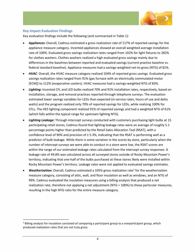
Key evaluation findings include the following (and summarized in Table 1):
Appliances: Overall, Cadmus estimated a gross realization rate of 117% of reported savings for the
appliance measure category. Incented appliances showed an overall weighted average installation
rate of 100%. Evaluated gross savings realization rates ranged from 102% for light fixtures to 282%
for clothes washers. Clothes washers realized a high evaluated gross savings mainly due to
differences in the baselines between reported and evaluated savings (current practice baseline vs.
federal standard baseline). Appliance measures had a savings-weighted net-to-gross (NTG) of 81%.
HVAC: Overall, the HVAC measure category realized 104% of reported gross savings. Evaluated gross
savings realization rates ranged from 91% (gas furnace with an electrically commutated motor
[ECM]) to 112% (evaporative coolers). HVAC measures had a savings-weighted NTG of 83%.
Lighting: Incented CFL and LED bulbs realized 70% and 91% installation rates, respectively, based on
installation, storage, and removal practices reported through telephone surveys. The evaluation
estimated lower savings variables for LEDs than expected (in-service rates, hours-of use and delta
watts) and the program realized only 70% of reported savings for LEDs, while realizing 100% for
CFLs. The HES lighting component realized 91% of reported savings and had a weighted NTG of 61%
(which falls within the typical range for upstream lighting NTG).
Lighting Leakage: Through intercept surveys conducted with customers purchasing light bulbs at 15
participating retail stores, Cadmus found that lighting leakage rates were an average of roughly 5.1
percentage points higher than predicted by the Retail Sales Allocation Tool (RSAT), with a
confidence level of 90% and precision of ± 5.3%, indicating that the RSAT is performing well as a
predictor of bulb leakage. While there is some variation in the scores by store, particularly when the
number of intercept surveys we were able to conduct in a store were low, the RSAT scores are
within the range of our estimated leakage rates calculated from the intercept survey responses. A
leakage rate of 49.8% was calculated across all surveyed stores outside of Rocky Mountain Power’s
territory, indicating that one-half of the bulbs purchased at these stores likely were installed within
Rocky Mountain Power’s territory. Leakage rates were not applied to evaluated savings estimates.
Weatherization: Overall, Cadmus estimated a 105% gross realization rate2 for the weatherization
measure category, consisting of attic, wall, and floor insulation as well as windows, and an NTG of
99%. Cadmus evaluated the insulation measures using a billing analysis that produced a net
realization rate, therefore not applying a net adjustment (NTG = 100%) to those particular measures,
resulting in the high NTG ratio for the entire measure category.
2 Billing analysis for insulation consisted of comparing a participant group to a nonparticipant group, which produced realization rates that are not truly gross.
7
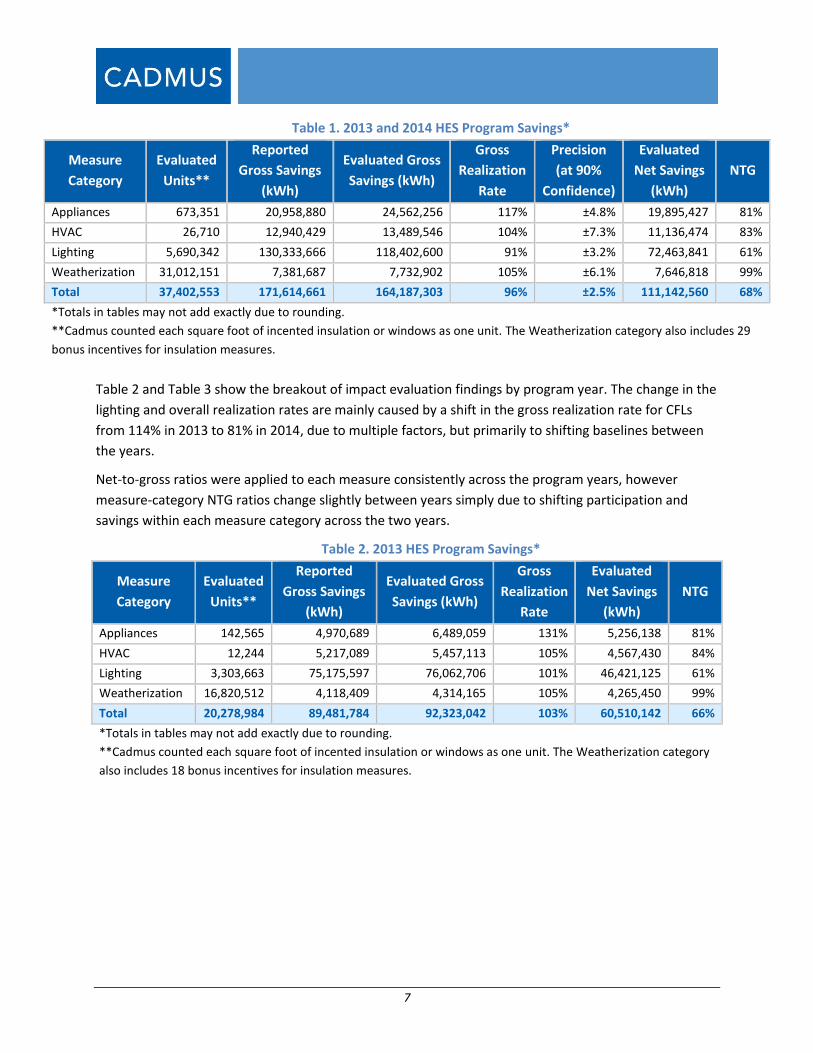
Table 1. 2013 and 2014 HES Program Savings*
Measure
Category
Evaluated
Units**
Reported
Gross Savings
(kWh)
Evaluated Gross
Savings (kWh)
Gross
Realization
Rate
Precision
(at 90%
Confidence)
Evaluated
Net Savings
(kWh)
NTG
Appliances 673,351 20,958,880 24,562,256 117% ±4.8% 19,895,427 81%
HVAC 26,710 12,940,429 13,489,546 104% ±7.3% 11,136,474 83%
Lighting 5,690,342 130,333,666 118,402,600 91% ±3.2% 72,463,841 61%
Weatherization 31,012,151 7,381,687 7,732,902 105% ±6.1% 7,646,818 99%
Total 37,402,553 171,614,661 164,187,303 96% ±2.5% 111,142,560 68%
*Totals in tables may not add exactly due to rounding.
**Cadmus counted each square foot of incented insulation or windows as one unit. The Weatherization category also includes 29
bonus incentives for insulation measures.
Table 2 and Table 3 show the breakout of impact evaluation findings by program year. The change in the
lighting and overall realization rates are mainly caused by a shift in the gross realization rate for CFLs
from 114% in 2013 to 81% in 2014, due to multiple factors, but primarily to shifting baselines between
the years.
Net-to-gross ratios were applied to each measure consistently across the program years, however
measure-category NTG ratios change slightly between years simply due to shifting participation and
savings within each measure category across the two years.
Table 2. 2013 HES Program Savings*
Measure
Category
Evaluated
Units**
Reported
Gross Savings
(kWh)
Evaluated Gross
Savings (kWh)
Gross
Realization
Rate
Evaluated
Net Savings
(kWh)
NTG
Appliances 142,565 4,970,689 6,489,059 131% 5,256,138 81%
HVAC 12,244 5,217,089 5,457,113 105% 4,567,430 84%
Lighting 3,303,663 75,175,597 76,062,706 101% 46,421,125 61%
Weatherization 16,820,512 4,118,409 4,314,165 105% 4,265,450 99%
Total 20,278,984 89,481,784 92,323,042 103% 60,510,142 66%
*Totals in tables may not add exactly due to rounding.
**Cadmus counted each square foot of incented insulation or windows as one unit. The Weatherization category
also includes 18 bonus incentives for insulation measures.
8
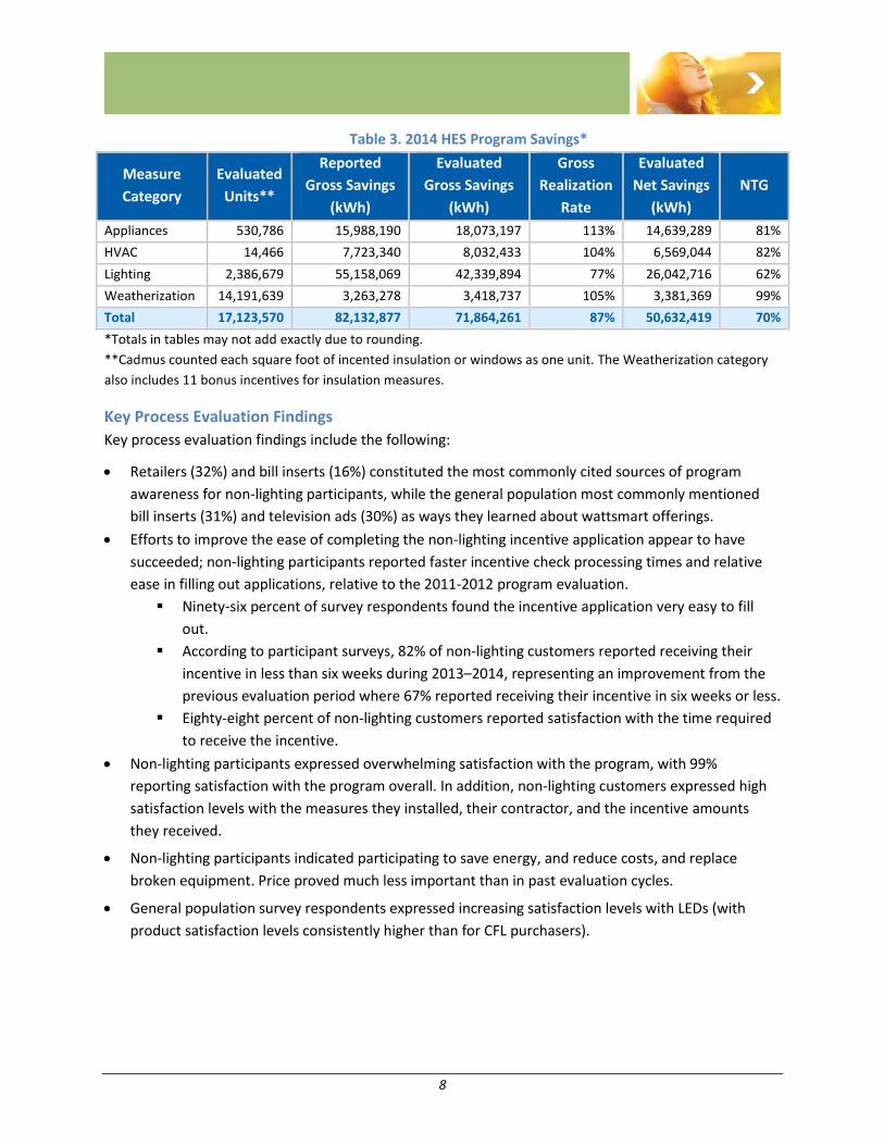
Table 3. 2014 HES Program Savings*
Measure
Category
Evaluated
Units**
Reported
Gross Savings
(kWh)
Evaluated
Gross Savings
(kWh)
Gross
Realization
Rate
Evaluated
Net Savings
(kWh)
NTG
Appliances 530,786 15,988,190 18,073,197 113% 14,639,289 81%
HVAC 14,466 7,723,340 8,032,433 104% 6,569,044 82%
Lighting 2,386,679 55,158,069 42,339,894 77% 26,042,716 62%
Weatherization 14,191,639 3,263,278 3,418,737 105% 3,381,369 99%
Total 17,123,570 82,132,877 71,864,261 87% 50,632,419 70%
*Totals in tables may not add exactly due to rounding.
**Cadmus counted each square foot of incented insulation or windows as one unit. The Weatherization category
also includes 11 bonus incentives for insulation measures.
Key Process Evaluation Findings
Key process evaluation findings include the following:
Retailers (32%) and bill inserts (16%) constituted the most commonly cited sources of program
awareness for non-lighting participants, while the general population most commonly mentioned
bill inserts (31%) and television ads (30%) as ways they learned about wattsmart offerings.
Efforts to improve the ease of completing the non-lighting incentive application appear to have
succeeded; non-lighting participants reported faster incentive check processing times and relative
ease in filling out applications, relative to the 2011-2012 program evaluation.
Ninety-six percent of survey respondents found the incentive application very easy to fill
out.
According to participant surveys, 82% of non-lighting customers reported receiving their
incentive in less than six weeks during 2013–2014, representing an improvement from the
previous evaluation period where 67% reported receiving their incentive in six weeks or less.
Eighty-eight percent of non-lighting customers reported satisfaction with the time required
to receive the incentive.
Non-lighting participants expressed overwhelming satisfaction with the program, with 99%
reporting satisfaction with the program overall. In addition, non-lighting customers expressed high
satisfaction levels with the measures they installed, their contractor, and the incentive amounts
they received.
Non-lighting participants indicated participating to save energy, and reduce costs, and replace
broken equipment. Price proved much less important than in past evaluation cycles.
General population survey respondents expressed increasing satisfaction levels with LEDs (with
product satisfaction levels consistently higher than for CFL purchasers).
9
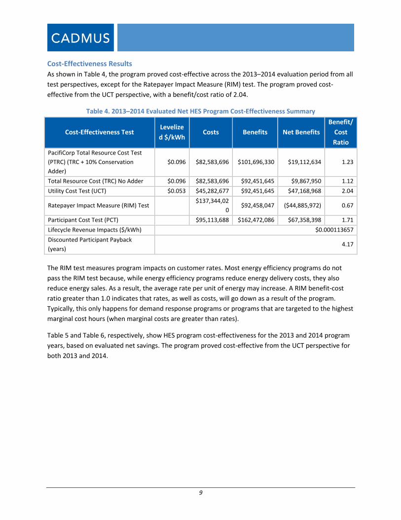
Cost-Effectiveness Results
As shown in Table 4, the program proved cost-effective across the 2013–2014 evaluation period from all
test perspectives, except for the Ratepayer Impact Measure (RIM) test. The program proved cost-
effective from the UCT perspective, with a benefit/cost ratio of 2.04.
Table 4. 2013–2014 Evaluated Net HES Program Cost-Effectiveness Summary
Cost-Effectiveness Test Levelize
d $/kWh Costs Benefits Net Benefits
Benefit/
Cost
Ratio
PacifiCorp Total Resource Cost Test
(PTRC) (TRC + 10% Conservation
Adder)
$0.096 $82,583,696 $101,696,330 $19,112,634 1.23
Total Resource Cost (TRC) No Adder $0.096 $82,583,696 $92,451,645 $9,867,950 1.12
Utility Cost Test (UCT) $0.053 $45,282,677 $92,451,645 $47,168,968 2.04
Ratepayer Impact Measure (RIM) Test $137,344,02
0 $92,458,047 ($44,885,972) 0.67
Participant Cost Test (PCT) $95,113,688 $162,472,086 $67,358,398 1.71
Lifecycle Revenue Impacts ($/kWh) $0.000113657
Discounted Participant Payback
(years) 4.17
The RIM test measures program impacts on customer rates. Most energy efficiency programs do not
pass the RIM test because, while energy efficiency programs reduce energy delivery costs, they also
reduce energy sales. As a result, the average rate per unit of energy may increase. A RIM benefit-cost
ratio greater than 1.0 indicates that rates, as well as costs, will go down as a result of the program.
Typically, this only happens for demand response programs or programs that are targeted to the highest
marginal cost hours (when marginal costs are greater than rates).
Table 5 and Table 6, respectively, show HES program cost-effectiveness for the 2013 and 2014 program
years, based on evaluated net savings. The program proved cost-effective from the UCT perspective for
both 2013 and 2014.
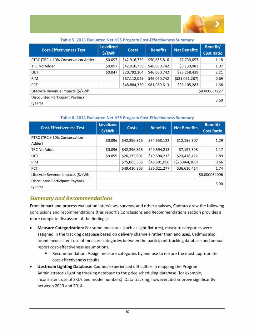
10
Table 5. 2013 Evaluated Net HES Program Cost-Effectiveness Summary
Cost-Effectiveness Test Levelized
$/kWh Costs Benefits Net Benefits
Benefit/
Cost Ratio
PTRC (TRC + 10% Conservation Adder) $0.097 $42,916,759 $50,655,816 $7,739,057 1.18
TRC No Adder $0.097 $42,916,759 $46,050,742 $3,133,983 1.07
UCT $0.047 $20,792,304 $46,050,742 $25,258,439 2.21
RIM $67,112,029 $46,050,742 ($21,061,287) 0.69
PCT $48,884,330 $81,989,613 $33,105,283 1.68
Lifecycle Revenue Impacts ($/kWh) $0.000054127
Discounted Participant Payback
(years) 3.60
Table 6. 2014 Evaluated Net HES Program Cost-Effectiveness Summary
Cost-Effectiveness Test Levelized
$/kWh Costs Benefits Net Benefits
Benefit/
Cost Ratio
PTRC (TRC + 10% Conservation
Adder) $0.096 $42,396,815 $54,553,122 $12,156,307 1.29
TRC No Adder $0.096 $42,396,815 $49,594,213 $7,197,398 1.17
UCT $0.059 $26,175,801 $49,594,213 $23,418,412 1.89
RIM $75,065,356 $49,601,056 ($25,464,300) 0.66
PCT $49,410,863 $86,021,277 $36,610,414 1.74
Lifecycle Revenue Impacts ($/kWh) $0.000064096
Discounted Participant Payback
(years) 3.90
Summary and Recommendations From impact and process evaluation interviews, surveys, and other analyses, Cadmus drew the following
conclusions and recommendations (this report’s Conclusions and Recommendations section provides a
more complete discussion of the findings):
Measure Categorization: For some measures (such as light fixtures), measure categories were
assigned in the tracking database based on delivery channels rather than end uses. Cadmus also
found inconsistent use of measure categories between the participant tracking database and annual
report cost-effectiveness assumptions.
Recommendation: Assign measure categories by end use to ensure the most appropriate
cost-effectiveness results.
Upstream Lighting Database: Cadmus experienced difficulties in mapping the Program
Administrator’s lighting tracking database to the price scheduling database (for example,
inconsistent use of SKUs and model numbers). Data tracking, however, did improve significantly
between 2013 and 2014.
11
Recommendation: Track all data in a consistent manner across each program evaluation
period (i.e. 2015-2016, 2016-2017 etc.).
Lighting Cross-Sector Sales: Cadmus estimated that 3.9% of efficient bulbs purchased at retail stores
ultimately would be installed in commercial applications. Bulbs installed in commercial spaces
produce higher first-year savings than bulbs installed in a residential space as commercial locations
typically have a higher daily use of bulbs than residential locations (i.e., higher HOU). Currently,
Rocky Mountain Power does not account for cross-sector sales from the upstream lighting
incentives.
Recommendation: Consider accounting for commercial installation of upstream bulbs in the
reported savings.
Nonparticipant Spillover: Nonparticipant spillover results in energy savings caused by, but not
rebated through, a utility’s demand-side management activities. Through responses to the general
population survey, Cadmus estimated nonparticipant spillover as 1% of HES program savings. As the
estimation of these savings is relatively new in the industry, and as savings have not been assessed
in previous program evaluations, Cadmus did not apply this adjustment.
Recommendation: Consider allowing nonparticipant spillover analysis to be an integral
component of NTG estimations for all programs.
Lighting Leakage: The RSAT allocation score is performing well in Utah. Through intercept surveys
conducted with customers purchasing light bulbs at 15 participating retail stores, Cadmus found that
lighting leakage rates were an average of roughly 5.1 points higher than predicted by the RSAT, with
a confidence level of 90% and precision of ± 5.3%, indicating that the RSAT is performing well as a
predictor of bulb leakage. While there is some variation in the scores by store, particularly when the
number of intercept surveys we were able to conduct in a store were low, the RSAT scores are
within the range of our estimated leakage rates calculated from the intercept survey responses.
Recommendation: Rocky Mountain Power should continue using the RSAT to determine
which stores in their territory should be included as participating stores in the program.
Lighting Spillover: This evaluation examined a portion of participant spillover found from the
upstream lighting store intercept leakage survey, however, it was not an exhaustive view of spillover
since the sample was designed to capture leakage and not spillover. Stores were chosen for
intercepts based on their RSAT scores, instead of randomly sampled within all participating stores
within the Rocky Mountain Power territory, which is what would be required to calculate spillover.
Recommendation: Consider additional studies to quantify spillover and market
transformation for use in lighting NTG calculations.
Customer Outreach: Bill inserts and retailers constituted the most commonly cited program
awareness sources for non-lighting participants. While the website was an influential source of
general wattsmart awareness for the general population of customers, it did not serve as a main
participation driver for the non-lighting program.
Recommendation: Continue to pursue a multi-touch marketing strategy, using a mix of bill
inserts and retailer/contractor training. Given the large percentage of customers who
learned of wattsmart offerings through bill inserts, examine the proportion of customers
12
selecting to receive online bills and ensure these online channels proportionately advertise
the programs with the messages that motivated customers to participate: long-lasting
products, saving energy, replacing equipment and reducing costs.
Application Processing: Despite substantive improvements in participant-reported application
processing times, reported processing times remained lengthy for duct sealing and insulation and
attic, floor and wall insulation, indicating opportunities for improvements for these specific
measures.
Recommendation: Continue to review methods for simplifying the applications, particularly
for duct sealing and insulation applications which have been prone to greater errors.
Implement additional training for HVAC and weatherization contractors to help mitigate this
issue by covering the data points required for a complete application and how to best
support a customer who chooses to fill out the application, and explore making duct sealing
and insulation an online application to reduce errors.
Satisfaction with Program Experience: While Cadmus was not able to verify the efficacy of the
program administrator’s efforts to reach out to non-registered contractors who worked with rebate-
seeking participants, the program’s efforts to mitigate contractor confusion regarding tariff changes
appeared to support the customers’ reported satisfaction.
Recommendation: Continue regular trainings with trade allies (e.g., distributors, retailers,
sales associates, contractors), updating them on tariff changes and, where appropriate,
supporting them with sales and marketing training. Analyze success of efforts to register
non-registered contractors who worked with rebate participants within 90 days to
determine whether the additional outreach mitigated the number of rejected applications
due to non-qualified contractors.

13
Introduction
Program Description CLEAResult (formerly Portland Energy Conservation Inc.) administered the program during the 2013-
2014 period, providing prescriptive incentives to residential customers who purchased qualifying, high-
efficiency appliances, heating, ventilation, and air conditioning (HVAC) and weatherization measures.
The HES program also included an upstream lighting component, with incentives applied to eligible CFLs
and LEDs at the manufacturer level, providing discounted high-efficiency lighting options. In early 2015,
light fixtures moved from a prescriptive offering to an upstream delivery.
The HES program offered the following measures for part or all of the evaluation period:
Appliances:
Ceiling fan
Clothes washer
Dishwasher
Electric water heater
Freezer
Light fixture
Portable evaporative cooler
Refrigerator
Room air conditioner
HVAC:
Central air conditioner best practice installations
Central air conditioner proper sizing
Central air conditioners
Duct sealing and insulation
Evaporative cooler (permanently installed, premium, ducted, and replacement)
Gas furnaces with an electronically commutated motor (ECM)
Heat pump water heater
Lighting
CFLs
LEDs
Weatherization:
Insulation (attic, floor, and wall)
Windows

14
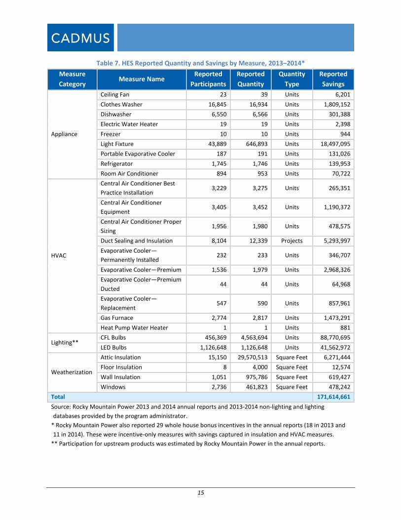
Program Participation During the 2013–2014 HES program years, Rocky Mountain Power provided prescriptive incentives to
over 60,000 residential customers and provided upstream discounts for over 6,000,000 products. Table
7 shows participation and savings by measures and measure categories for this period.
15
Table 7. HES Reported Quantity and Savings by Measure, 2013–2014*
Measure
Category Measure Name
Reported
Participants
Reported
Quantity
Quantity
Type
Reported
Savings
Appliance
Ceiling Fan 23 39 Units 6,201
Clothes Washer 16,845 16,934 Units 1,809,152
Dishwasher 6,550 6,566 Units 301,388
Electric Water Heater 19 19 Units 2,398
Freezer 10 10 Units 944
Light Fixture 43,889 646,893 Units 18,497,095
Portable Evaporative Cooler 187 191 Units 131,026
Refrigerator 1,745 1,746 Units 139,953
Room Air Conditioner 894 953 Units 70,722
HVAC
Central Air Conditioner Best
Practice Installation 3,229 3,275 Units 265,351
Central Air Conditioner
Equipment 3,405 3,452 Units 1,190,372
Central Air Conditioner Proper
Sizing 1,956 1,980 Units 478,575
Duct Sealing and Insulation 8,104 12,339 Projects 5,293,997
Evaporative Cooler—
Permanently Installed 232 233 Units 346,707
Evaporative Cooler—Premium 1,536 1,979 Units 2,968,326
Evaporative Cooler—Premium
Ducted 44 44 Units 64,968
Evaporative Cooler—
Replacement 547 590 Units 857,961
Gas Furnace 2,774 2,817 Units 1,473,291
Heat Pump Water Heater 1 1 Units 881
Lighting** CFL Bulbs 456,369 4,563,694 Units 88,770,695
LED Bulbs 1,126,648 1,126,648 Units 41,562,972
Weatherization
Attic Insulation 15,150 29,570,513 Square Feet 6,271,444
Floor Insulation 8 4,000 Square Feet 12,574
Wall Insulation 1,051 975,786 Square Feet 619,427
Windows 2,736 461,823 Square Feet 478,242
Total 171,614,661
Source: Rocky Mountain Power 2013 and 2014 annual reports and 2013-2014 non-lighting and lighting
databases provided by the program administrator.
* Rocky Mountain Power also reported 29 whole house bonus incentives in the annual reports (18 in 2013 and
11 in 2014). These were incentive-only measures with savings captured in insulation and HVAC measures.
** Participation for upstream products was estimated by Rocky Mountain Power in the annual reports.
16
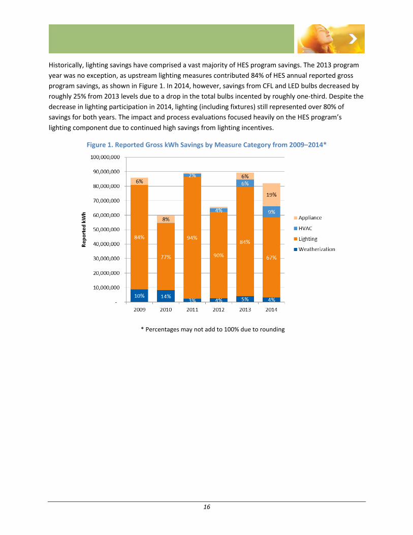
Historically, lighting savings have comprised a vast majority of HES program savings. The 2013 program
year was no exception, as upstream lighting measures contributed 84% of HES annual reported gross
program savings, as shown in Figure 1. In 2014, however, savings from CFL and LED bulbs decreased by
roughly 25% from 2013 levels due to a drop in the total bulbs incented by roughly one-third. Despite the
decrease in lighting participation in 2014, lighting (including fixtures) still represented over 80% of
savings for both years. The impact and process evaluations focused heavily on the HES program’s
lighting component due to continued high savings from lighting incentives.
Figure 1. Reported Gross kWh Savings by Measure Category from 2009–2014*
* Percentages may not add to 100% due to rounding
17
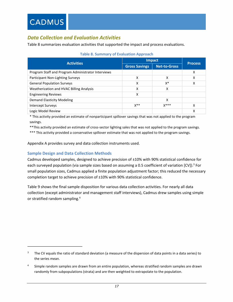
Data Collection and Evaluation Activities Table 8 summarizes evaluation activities that supported the impact and process evaluations.
Table 8. Summary of Evaluation Approach
Activities Impact
Process Gross Savings Net-to-Gross
Program Staff and Program Administrator Interviews X
Participant Non-Lighting Surveys X X X
General Population Surveys X X* X
Weatherization and HVAC Billing Analysis X X
Engineering Reviews X
Demand Elasticity Modeling X
Intercept Surveys X** X*** X
Logic Model Review X
* This activity provided an estimate of nonparticipant spillover savings that was not applied to the program
savings.
**This activity provided an estimate of cross-sector lighting sales that was not applied to the program savings.
*** This activity provided a conservative spillover estimate that was not applied to the program savings.
Appendix A provides survey and data collection instruments used.
Sample Design and Data Collection Methods
Cadmus developed samples, designed to achieve precision of ±10% with 90% statistical confidence for
each surveyed population (via sample sizes based on assuming a 0.5 coefficient of variation [CV]).3 For
small population sizes, Cadmus applied a finite population adjustment factor; this reduced the necessary
completion target to achieve precision of ±10% with 90% statistical confidence.
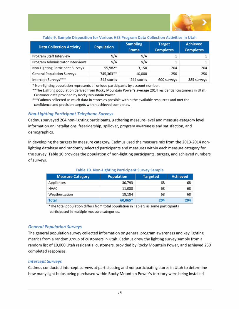
Table 9 shows the final sample disposition for various data collection activities. For nearly all data
collection (except administrator and management staff interviews), Cadmus drew samples using simple
or stratified random sampling.4
3 The CV equals the ratio of standard deviation (a measure of the dispersion of data points in a data series) to
the series mean.
4 Simple random samples are drawn from an entire population, whereas stratified random samples are drawn
randomly from subpopulations (strata) and are then weighted to extrapolate to the population.
18
Table 9. Sample Disposition for Various HES Program Data Collection Activities in Utah
Data Collection Activity Population Sampling
Frame
Target
Completes
Achieved
Completes
Program Staff Interview N/A N/A 1 1
Program Administrator Interviews N/A N/A 1 1
Non-Lighting Participant Surveys 55,982* 3,150 204 204
General Population Surveys 745,363** 10,000 250 250
Intercept Surveys*** 345 stores 244 stores 600 surveys 385 surveys
* Non-lighting population represents all unique participants by account number. **The Lighting population derived from Rocky Mountain Power’s average 2014 residential customers in Utah.
Customer data provided by Rocky Mountain Power. ***Cadmus collected as much data in stores as possible within the available resources and met the
confidence and precision targets within achieved completes.
Non-Lighting Participant Telephone Surveys
Cadmus surveyed 204 non-lighting participants, gathering measure-level and measure-category level
information on installations, freeridership, spillover, program awareness and satisfaction, and
demographics.
In developing the targets by measure category, Cadmus used the measure mix from the 2013-2014 non-
lighting database and randomly selected participants and measures within each measure category for
the survey. Table 10 provides the population of non-lighting participants, targets, and achieved numbers
of surveys.
Table 10. Non-Lighting Participant Survey Sample
Measure Category Population Targeted Achieved
Appliances 30,793 68 68
HVAC 11,088 68 68
Weatherization 18,184 68 68
Total 60,065* 204 204
*The total population differs from total population in Table 9 as some participants
participated in multiple measure categories.
General Population Surveys
The general population survey collected information on general program awareness and key lighting
metrics from a random group of customers in Utah. Cadmus drew the lighting survey sample from a
random list of 10,000 Utah residential customers, provided by Rocky Mountain Power, and achieved 250
completed responses.
Intercept Surveys
Cadmus conducted intercept surveys at participating and nonparticipating stores in Utah to determine
how many light bulbs being purchased within Rocky Mountain Power’s territory were being installed
19
outside of the territory (leakage), with the primary purpose to evaluate the accuracy of the Retail Sales
Allocation Tool (RSAT).
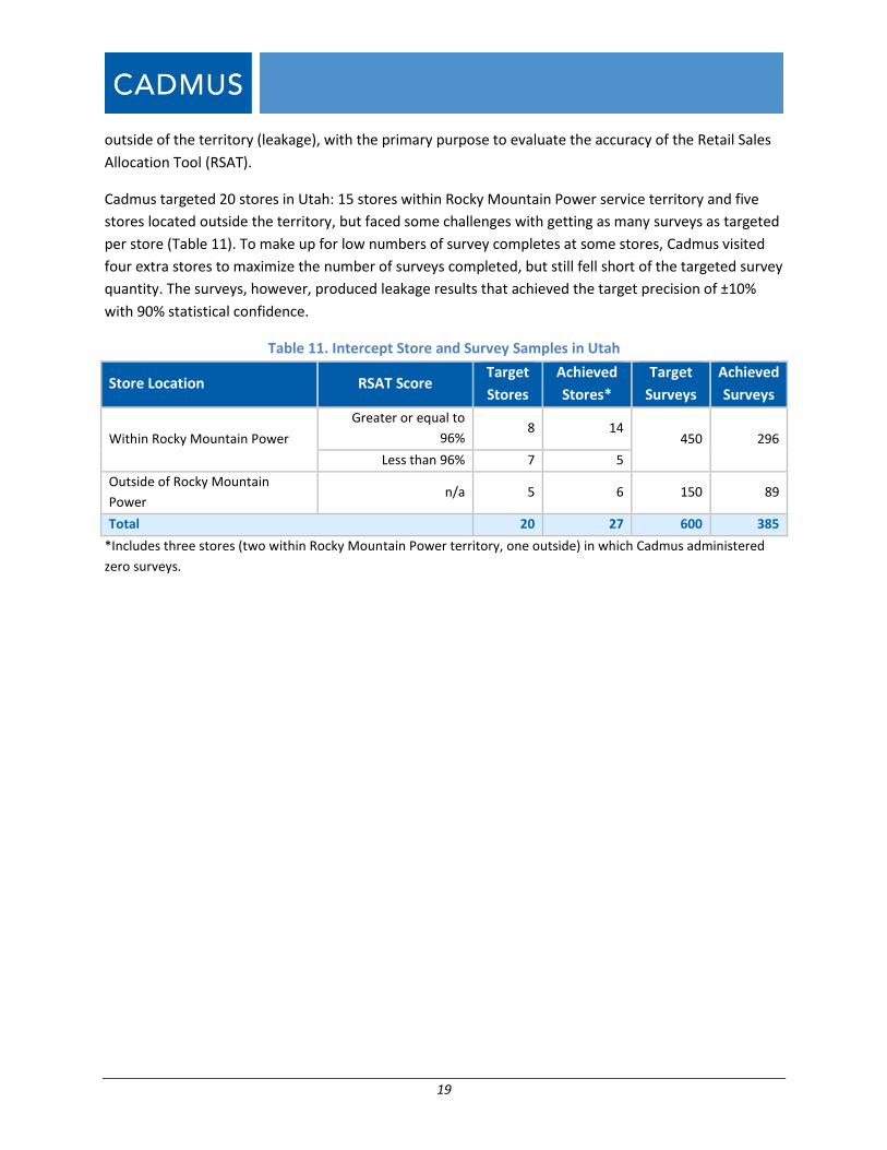
Cadmus targeted 20 stores in Utah: 15 stores within Rocky Mountain Power service territory and five
stores located outside the territory, but faced some challenges with getting as many surveys as targeted
per store (Table 11). To make up for low numbers of survey completes at some stores, Cadmus visited
four extra stores to maximize the number of surveys completed, but still fell short of the targeted survey
quantity. The surveys, however, produced leakage results that achieved the target precision of ±10%
with 90% statistical confidence.
Table 11. Intercept Store and Survey Samples in Utah
Store Location RSAT Score Target
Stores
Achieved
Stores*
Target
Surveys
Achieved
Surveys
Within Rocky Mountain Power
Greater or equal to
96% 8 14
450 296
Less than 96% 7 5
Outside of Rocky Mountain
Power n/a 5 6 150 89
Total 20 27 600 385
*Includes three stores (two within Rocky Mountain Power territory, one outside) in which Cadmus administered
zero surveys.

20
Impact Evaluation
This chapter provides impact evaluation findings for the HES program, based on Cadmus’ data analysis,
which used the following methods:
Participant surveys
General population surveys
Intercept surveys
Billing analysis
Engineering reviews
Elasticity modeling
This report presents two evaluated saving values: gross savings and net savings. To determine evaluated
net savings, Cadmus applied all four steps shown in Table 12 and described in the following text.
Reported gross savings are electricity savings (kWh) that Rocky Mountain Power reported in the 2013
and 2014 Rocky Mountain Power Energy Efficiency and Peak Reduction Annual Reports (annual
reports).5
Table 12. Impact Steps to Determine Evaluated Net Savings
Savings Estimate Step Action
Evaluated Gross
Savings
1 Tracking Database Review: validate accuracy of data in the participant
database
2 Verification: Adjust gross savings with the actual installation rate
3 Unit Energy Savings: Validate saving calculations (i.e., billing analysis and
engineering reviews)
Evaluated Net Savings 4 Attribution: Apply net-to-gross adjustments
Step one (verify participant database) included reviewing the program tracking database to ensure
participants and reported savings matched 2013 and 2014 annual reports.
Step two (adjust gross savings with the actual installation rate) determined the number of program
measures installed and remaining installed. Cadmus determined this value through telephone surveys.
5 Rocky Mountain Power Utah Annual Reports:
2013 - http://www.pacificorp.com/content/dam/pacificorp/doc/Energy_Sources/Demand_Side_Management/2014/2013-UT-Annual-Report-FINAL-Report-051614.pdf
2014 - http://www.pacificorp.com/content/dam/pacificorp/doc/Energy_Sources/Demand_Side_Management/2015/UT_2014-Annual-Report_FINAL042915.pdf
21
Step three (estimate gross unit energy savings [UES]) included reviews of measure saving assumptions,
equations, and inputs (e.g., engineering reviews for lighting and appliances, billing analysis for
weatherization and HVAC measures).
The first three steps determined evaluated gross savings. The fourth step (applying net adjustments)
determined evaluated net savings. Cadmus calculated the net saving adjustments using results from
customer self-response and demand elasticity modeling.
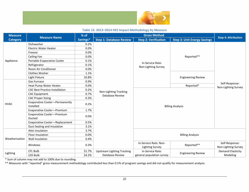
Table 13 outlines the methodology for each gross and net savings step, by measure, in the 2013–2014
HES program.
22
Table 13. 2013–2014 HES Impact Methodology by Measure
Measure Category
Measure Name % of
Savings*
Gross Method Step 4: Attribution
Step 1: Database Review Step 2: Verification Step 3: Unit Energy Savings
Appliance
Dishwasher 0.2%
Non-Lighting Tracking Database Review
In-Service Rate: Non-Lighting Survey
Reported**
Self-Response: Non-Lighting Survey
Electric Water Heater 0.0%
Freezer 0.0%
Ceiling Fan 0.0%
Portable Evaporative Cooler 0.1%
Refrigerator 0.1%
Room Air Conditioner 0.0%
Clothes Washer 1.1%
Engineering Review Light Fixture 10.8%
HVAC
Gas Furnace 0.9%
Heat Pump Water Heater 0.0% Reported*
CAC Best Practice Installation 0.2%
Billing Analysis
CAC Equipment 0.7%
CAC Proper Sizing 0.3%
Evaporative Cooler—Permanently Installed
0.2%
Evaporative Cooler—Premium 1.7%
Evaporative Cooler—Premium Ducted
0.0%
Evaporative Cooler—Replacement 0.5%
Duct Sealing and Insulation 3.1%
Weatherization
Attic Insulation 3.7%
Billing Analysis Floor Insulation 0.0%
Wall Insulation 0.4%
Windows 0.3% In-Service Rate: Non-
Lighting Survey Reported**
Self-Response: Non-Lighting Survey
Lighting CFL Bulb 51.7% Upstream Lighting Tracking
Database Review In-Service Rate:
general population survey Engineering Review
Demand Elasticity Modeling LED Bulb 24.2%
* Sum of column may not add to 100% due to rounding. ** Measures with “reported” gross measurement methodology contributed less than 0.5% of program savings and did not qualify for measurement analysis.
23
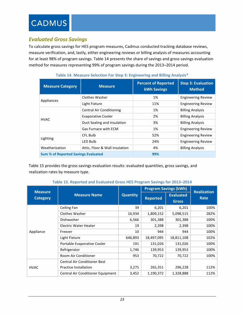
Evaluated Gross Savings To calculate gross savings for HES program measures, Cadmus conducted tracking database reviews,
measure verification, and, lastly, either engineering reviews or billing analysis of measures accounting
for at least 98% of program savings. Table 14 presents the share of savings and gross savings evaluation
method for measures representing 99% of program savings during the 2013–2014 period.
Table 14. Measure Selection For Step 3: Engineering and Billing Analysis*
Measure Category Measure Percent of Reported
kWh Savings
Step 3: Evaluation
Method
Appliances Clothes Washer 1% Engineering Review
Light Fixture 11% Engineering Review
HVAC
Central Air Conditioning 1% Billing Analysis
Evaporative Cooler 2% Billing Analysis
Duct Sealing and Insulation 3% Billing Analysis
Gas Furnace with ECM 1% Engineering Review
Lighting CFL Bulb 52% Engineering Review
LED Bulb 24% Engineering Review
Weatherization Attic, Floor & Wall Insulation 4% Billing Analysis
Sum % of Reported Savings Evaluated 99%
Table 15 provides the gross savings evaluation results: evaluated quantities, gross savings, and
realization rates by measure type.
Table 15. Reported and Evaluated Gross HES Program Savings for 2013–2014
Measure
Category Measure Name Quantity
Program Savings (kWh) Realization
Rate Reported Evaluated
Gross
Appliance
Ceiling Fan 39 6,201 6,201 100%
Clothes Washer 16,934 1,809,152 5,098,515 282%
Dishwasher 6,566 301,388 301,388 100%
Electric Water Heater 19 2,398 2,398 100%
Freezer 10 944 944 100%
Light Fixture 646,893 18,497,095 18,811,108 102%
Portable Evaporative Cooler 191 131,026 131,026 100%
Refrigerator 1,746 139,953 139,953 100%
Room Air Conditioner 953 70,722 70,722 100%
HVAC
Central Air Conditioner Best
Practice Installation 3,275 265,351 296,228 112%
Central Air Conditioner Equipment 3,452 1,190,372 1,328,888 112%

24
Measure
Category Measure Name Quantity
Program Savings (kWh) Realization
Rate Reported Evaluated
Gross
Central Air Conditioner Proper
Sizing 1,980 478,575 534,264 112%
Duct Sealing and Insulation 12,339 5,293,997 5,645,973 107%
Evaporative Cooler—Permanently
Installed 233 346,707 354,946 102%
Evaporative Cooler—Premium 1,979 2,968,326 3,038,862 102%
Evaporative Cooler—Premium
Ducted 44 64,968 66,512 102%
Evaporative Cooler—Replacement 590 857,961 878,349 102%
Gas Furnace with ECM 2,817 1,473,291 1,344,644 91%
Heat Pump Water Heater 1 881 881 100%
Lighting CFL Bulbs 4,563,694 88,770,695 89,199,262 100%
LED Bulbs 1,126,648 41,562,972 29,203,338 70%
Weatherization
*
Attic Insulation 29,570,513 6,271,444 6,590,506 105%
Floor Insulation 4,000 12,574 13,214 105%
Wall Insulation 975,786 619,427 650,940 105%
Windows 461,823 478,242 478,242 100%
Total** 171,614,661 164,187,303 96%
*Quantities for weatherization measures are in square feet.
**Savings may not add exactly to total row due to rounding.
Step 1: Tracking Database Reviews
The program administrator provided two tracking databases containing Utah data, covering all 2013 and
2014 participation for the two delivery methods: upstream (lighting) and downstream (non-lighting).
The upstream lighting measures database collected meaningful information, tracking lighting at a per-
bulb level and including information such as retailers, electric savings, purchased dates, and stock
keeping units (SKUs).6 Cadmus’ review of the database tracking for 2013 and 2014 found no
discrepancies in total reported quantities or total savings compared to the 2013 and 2014 annual
reports.
Cadmus also reviewed the program administrator’s tracking of 2013 and 2014 non-lighting measures.
This database collected measure-level information such as efficiency standards, quantities of units,
purchase dates, and incentive amounts. Cadmus found the total quantities and savings exactly matched
the 2013 and 2014 annual reports.
6 SKU numbers represent unique make and model indicators for a specific retailer.
25
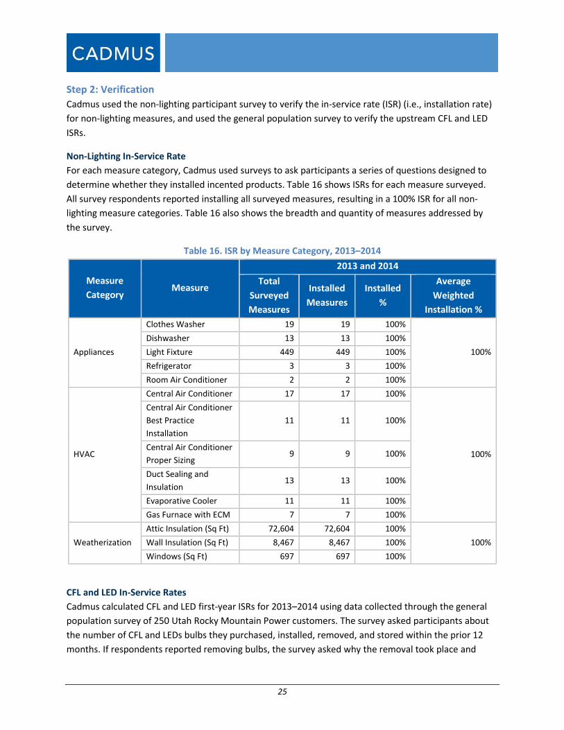
Step 2: Verification
Cadmus used the non-lighting participant survey to verify the in-service rate (ISR) (i.e., installation rate)
for non-lighting measures, and used the general population survey to verify the upstream CFL and LED
ISRs.
Non-Lighting In-Service Rate
For each measure category, Cadmus used surveys to ask participants a series of questions designed to
determine whether they installed incented products. Table 16 shows ISRs for each measure surveyed.
All survey respondents reported installing all surveyed measures, resulting in a 100% ISR for all non-
lighting measure categories. Table 16 also shows the breadth and quantity of measures addressed by
the survey.
Table 16. ISR by Measure Category, 2013–2014
Measure
Category Measure
2013 and 2014
Total
Surveyed
Measures
Installed
Measures
Installed
%
Average
Weighted
Installation %
Appliances
Clothes Washer 19 19 100%
100%
Dishwasher 13 13 100%
Light Fixture 449 449 100%
Refrigerator 3 3 100%
Room Air Conditioner 2 2 100%
HVAC
Central Air Conditioner 17 17 100%
100%
Central Air Conditioner
Best Practice
Installation
11 11 100%
Central Air Conditioner
Proper Sizing 9 9 100%
Duct Sealing and
Insulation 13 13 100%
Evaporative Cooler 11 11 100%
Gas Furnace with ECM 7 7 100%
Weatherization
Attic Insulation (Sq Ft) 72,604 72,604 100%
100% Wall Insulation (Sq Ft) 8,467 8,467 100%
Windows (Sq Ft) 697 697 100%
CFL and LED In-Service Rates
Cadmus calculated CFL and LED first-year ISRs for 2013–2014 using data collected through the general
population survey of 250 Utah Rocky Mountain Power customers. The survey asked participants about
the number of CFL and LEDs bulbs they purchased, installed, removed, and stored within the prior 12
months. If respondents reported removing bulbs, the survey asked why the removal took place and
26
adjusted the ISR accordingly. The calculated ISR does not account for installations occurring after the
first year of purchase. Appendix D of the 2011-2012 Rocky Mountain Power Home Energy Savings
Program Evaluation Report provides more information regarding second and third year ISRs. The
Uniform Methods Project (UMP) recommends adjusting (increasing) the ISR to account for bulbs initially
placed in storage that the customer will subsequently install in the years following the purchase.7 This
evaluation takes a conservative approach and claims savings attributed to just the first year of bulb
installations.
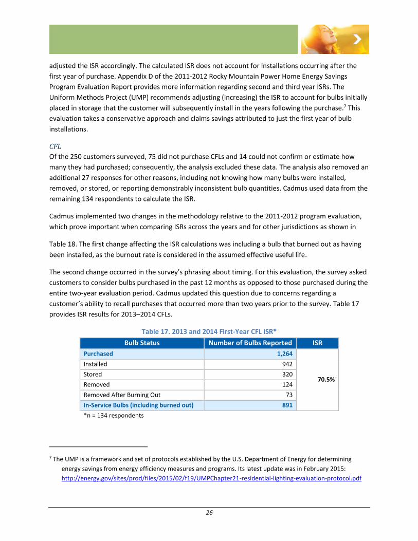
CFL
Of the 250 customers surveyed, 75 did not purchase CFLs and 14 could not confirm or estimate how
many they had purchased; consequently, the analysis excluded these data. The analysis also removed an
additional 27 responses for other reasons, including not knowing how many bulbs were installed,
removed, or stored, or reporting demonstrably inconsistent bulb quantities. Cadmus used data from the
remaining 134 respondents to calculate the ISR.
Cadmus implemented two changes in the methodology relative to the 2011-2012 program evaluation,
which prove important when comparing ISRs across the years and for other jurisdictions as shown in
Table 18. The first change affecting the ISR calculations was including a bulb that burned out as having
been installed, as the burnout rate is considered in the assumed effective useful life.
The second change occurred in the survey’s phrasing about timing. For this evaluation, the survey asked
customers to consider bulbs purchased in the past 12 months as opposed to those purchased during the
entire two-year evaluation period. Cadmus updated this question due to concerns regarding a
customer’s ability to recall purchases that occurred more than two years prior to the survey. Table 17
provides ISR results for 2013–2014 CFLs.
Table 17. 2013 and 2014 First-Year CFL ISR*
Bulb Status Number of Bulbs Reported ISR
Purchased 1,264
70.5%
Installed 942
Stored 320
Removed 124
Removed After Burning Out 73
In-Service Bulbs (including burned out) 891
*n = 134 respondents
7 The UMP is a framework and set of protocols established by the U.S. Department of Energy for determining
energy savings from energy efficiency measures and programs. Its latest update was in February 2015:
http://energy.gov/sites/prod/files/2015/02/f19/UMPChapter21-residential-lighting-evaluation-protocol.pdf

27
The revised formula for calculating the lighting ISR is:
𝐼𝑆𝑅 =𝐼𝑛𝑠𝑡𝑎𝑙𝑙𝑒𝑑 𝑖𝑛 𝑓𝑖𝑟𝑠𝑡 𝑦𝑒𝑎𝑟 − (𝑅𝑒𝑚𝑜𝑣𝑒𝑑 − 𝑅𝑒𝑚𝑜𝑣𝑒𝑑 𝐴𝑓𝑡𝑒𝑟 𝐵𝑢𝑟𝑛𝑖𝑛𝑔 𝑂𝑢𝑡)
𝑃𝑢𝑟𝑐ℎ𝑎𝑠𝑒𝑑
Table 18 compares first-year ISRs evaluated for similar programs across the country (and for some past
HES program evaluations in Utah). Utah’s CFL ISR has remained very stable over the past three
evaluations (e.g., 2009–2010, 2011–2012, and 2013–2014).
Table 18. Comparison of Evaluated First-Year CFL ISR Estimates
Source Data Collection Method Reported Year ISR
Midwest Utility 1 Self-reporting: determined by interview
during home inventory site visits 2016 86%
Avista 2012-2013 Electric Impact
Report Regional Technical Forum (RTF)* 2014 75%
Northeast Utility Self-Reporting: 200 telephone surveys 2012 73%
Rocky Mountain Power Utah 2013–
2014 HES Evaluation
Self-reporting: 134 in-territory lighting
surveys 2016 70%
Rocky Mountain Power Utah 2011–
2012 HES Evaluation
Self-reporting: 245 in-territory lighting
surveys 2014 69%
Rocky Mountain Power Utah 2009-
2010 HES Evaluation
Self-reporting: 250 in-territory lighting
surveys 2011 69%
Midwest Utility 2 Self-reporting: 301 customer surveys 2012 68%
*The RTF is an advisory committee in the northwest that develops standards to verify and evaluate
conservation savings.
LED
Cadmus calculated the first-year LED ISR using the same methodology and customer sample as those
used for CFLs. After filtering survey results for those purchased LEDs and provided reliable responses,
99 customers remained for inclusion in the LED ISR analysis. Table 19 summarizes the LED ISR results
and shows a higher, LED ISR compared to the CFL ISR. The higher cost of LEDs is most likely driving the
higher ISR: customers are more likely to install the bulb right after purchasing it if they just spent a
significant amount of money on the bulb (significant compared to CFL costs).
28
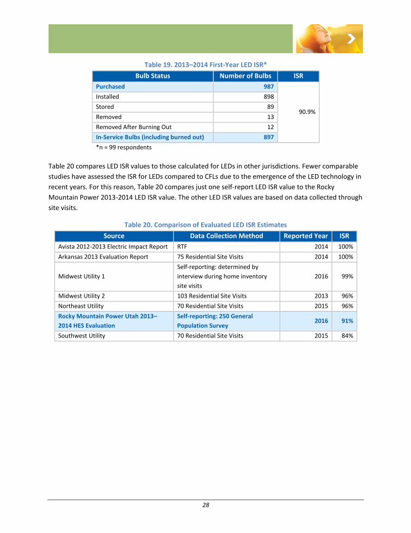
Table 19. 2013–2014 First-Year LED ISR*
Bulb Status Number of Bulbs ISR
Purchased 987
90.9%
Installed 898
Stored 89
Removed 13
Removed After Burning Out 12
In-Service Bulbs (including burned out) 897
*n = 99 respondents
Table 20 compares LED ISR values to those calculated for LEDs in other jurisdictions. Fewer comparable
studies have assessed the ISR for LEDs compared to CFLs due to the emergence of the LED technology in
recent years. For this reason, Table 20 compares just one self-report LED ISR value to the Rocky
Mountain Power 2013-2014 LED ISR value. The other LED ISR values are based on data collected through
site visits.
Table 20. Comparison of Evaluated LED ISR Estimates
Source Data Collection Method Reported Year ISR
Avista 2012-2013 Electric Impact Report RTF 2014 100%
Arkansas 2013 Evaluation Report 75 Residential Site Visits 2014 100%
Midwest Utility 1
Self-reporting: determined by
interview during home inventory
site visits
2016 99%
Midwest Utility 2 103 Residential Site Visits 2013 96%
Northeast Utility 70 Residential Site Visits 2015 96%
Rocky Mountain Power Utah 2013–
2014 HES Evaluation
Self-reporting: 250 General
Population Survey 2016 91%
Southwest Utility 70 Residential Site Visits 2015 84%
29
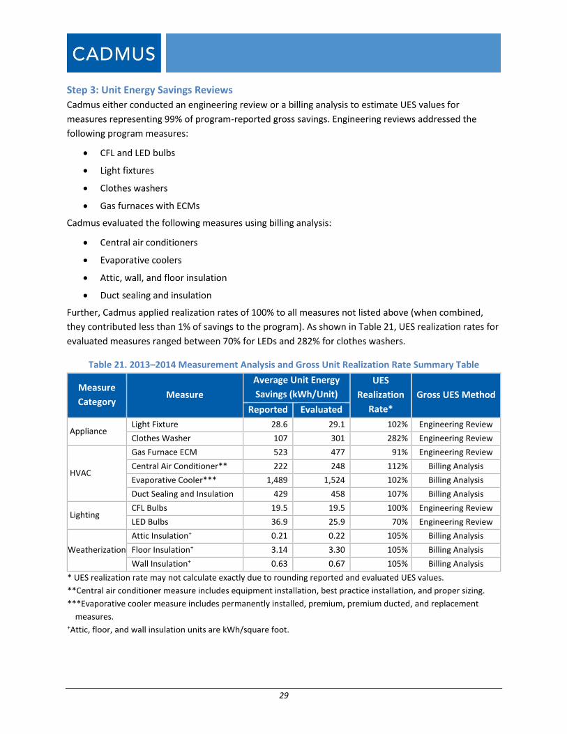
Step 3: Unit Energy Savings Reviews
Cadmus either conducted an engineering review or a billing analysis to estimate UES values for
measures representing 99% of program-reported gross savings. Engineering reviews addressed the
following program measures:
CFL and LED bulbs
Light fixtures
Clothes washers
Gas furnaces with ECMs
Cadmus evaluated the following measures using billing analysis:
Central air conditioners
Evaporative coolers
Attic, wall, and floor insulation
Duct sealing and insulation
Further, Cadmus applied realization rates of 100% to all measures not listed above (when combined,
they contributed less than 1% of savings to the program). As shown in Table 21, UES realization rates for
evaluated measures ranged between 70% for LEDs and 282% for clothes washers.
Table 21. 2013–2014 Measurement Analysis and Gross Unit Realization Rate Summary Table
Measure
Category Measure
Average Unit Energy
Savings (kWh/Unit)
UES
Realization
Rate*
Gross UES Method
Reported Evaluated
Appliance Light Fixture 28.6 29.1 102% Engineering Review
Clothes Washer 107 301 282% Engineering Review
HVAC
Gas Furnace ECM 523 477 91% Engineering Review
Central Air Conditioner** 222 248 112% Billing Analysis
Evaporative Cooler*** 1,489 1,524 102% Billing Analysis
Duct Sealing and Insulation 429 458 107% Billing Analysis
Lighting CFL Bulbs 19.5 19.5 100% Engineering Review
LED Bulbs 36.9 25.9 70% Engineering Review
Weatherization
Attic Insulation+ 0.21 0.22 105% Billing Analysis
Floor Insulation+ 3.14 3.30 105% Billing Analysis
Wall Insulation+ 0.63 0.67 105% Billing Analysis
* UES realization rate may not calculate exactly due to rounding reported and evaluated UES values.
**Central air conditioner measure includes equipment installation, best practice installation, and proper sizing.
***Evaporative cooler measure includes permanently installed, premium, premium ducted, and replacement
measures. +Attic, floor, and wall insulation units are kWh/square foot.
30
The following sections describe the methodology and results of the measurement activities for each
measure listed in Table 21.
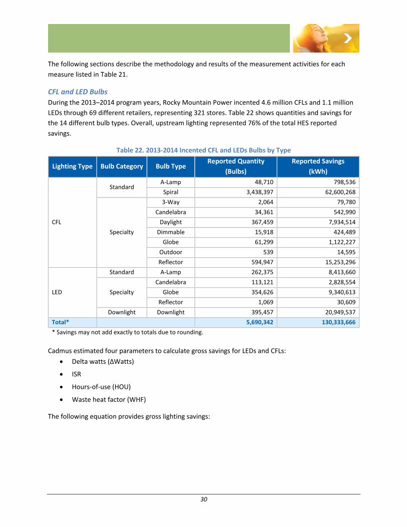
CFL and LED Bulbs
During the 2013–2014 program years, Rocky Mountain Power incented 4.6 million CFLs and 1.1 million
LEDs through 69 different retailers, representing 321 stores. Table 22 shows quantities and savings for
the 14 different bulb types. Overall, upstream lighting represented 76% of the total HES reported
savings.
Table 22. 2013-2014 Incented CFL and LEDs Bulbs by Type
Lighting Type Bulb Category Bulb Type Reported Quantity
(Bulbs)
Reported Savings
(kWh)
CFL
Standard A-Lamp 48,710 798,536
Spiral 3,438,397 62,600,268
Specialty
3-Way 2,064 79,780
Candelabra 34,361 542,990
Daylight 367,459 7,934,514
Dimmable 15,918 424,489
Globe 61,299 1,122,227
Outdoor 539 14,595
Reflector 594,947 15,253,296
LED
Standard A-Lamp 262,375 8,413,660
Specialty
Candelabra 113,121 2,828,554
Globe 354,626 9,340,613
Reflector 1,069 30,609
Downlight Downlight 395,457 20,949,537
Total* 5,690,342 130,333,666
* Savings may not add exactly to totals due to rounding.
Cadmus estimated four parameters to calculate gross savings for LEDs and CFLs:
Delta watts (ΔWatts)
ISR
Hours-of-use (HOU)
Waste heat factor (WHF)
The following equation provides gross lighting savings:
31
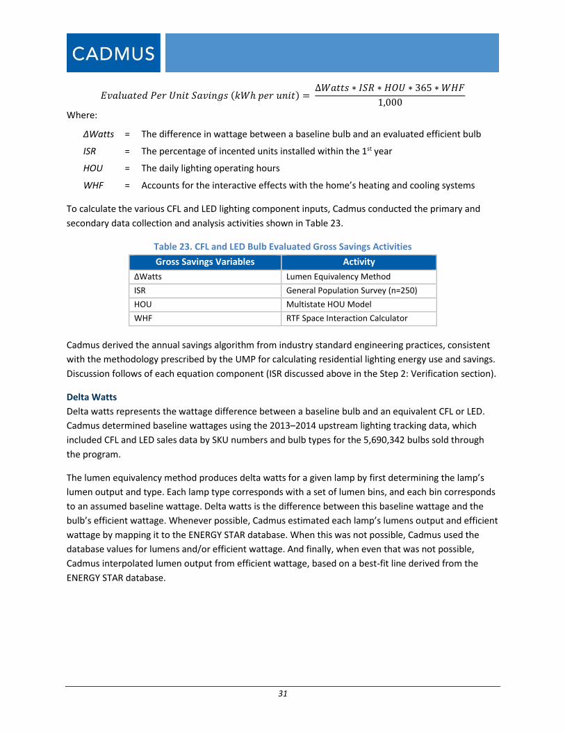
𝐸𝑣𝑎𝑙𝑢𝑎𝑡𝑒𝑑 𝑃𝑒𝑟 𝑈𝑛𝑖𝑡 𝑆𝑎𝑣𝑖𝑛𝑔𝑠 (𝑘𝑊ℎ 𝑝𝑒𝑟 𝑢𝑛𝑖𝑡) = ∆𝑊𝑎𝑡𝑡𝑠 ∗ 𝐼𝑆𝑅 ∗ 𝐻𝑂𝑈 ∗ 365 ∗ 𝑊𝐻𝐹
1,000
Where:
ΔWatts = The difference in wattage between a baseline bulb and an evaluated efficient bulb
ISR = The percentage of incented units installed within the 1st year
HOU = The daily lighting operating hours
WHF = Accounts for the interactive effects with the home’s heating and cooling systems
To calculate the various CFL and LED lighting component inputs, Cadmus conducted the primary and
secondary data collection and analysis activities shown in Table 23.
Table 23. CFL and LED Bulb Evaluated Gross Savings Activities
Gross Savings Variables Activity
ΔWatts Lumen Equivalency Method
ISR General Population Survey (n=250)
HOU Multistate HOU Model
WHF RTF Space Interaction Calculator
Cadmus derived the annual savings algorithm from industry standard engineering practices, consistent
with the methodology prescribed by the UMP for calculating residential lighting energy use and savings.
Discussion follows of each equation component (ISR discussed above in the Step 2: Verification section).
Delta Watts
Delta watts represents the wattage difference between a baseline bulb and an equivalent CFL or LED.
Cadmus determined baseline wattages using the 2013–2014 upstream lighting tracking data, which
included CFL and LED sales data by SKU numbers and bulb types for the 5,690,342 bulbs sold through
the program.
The lumen equivalency method produces delta watts for a given lamp by first determining the lamp’s
lumen output and type. Each lamp type corresponds with a set of lumen bins, and each bin corresponds
to an assumed baseline wattage. Delta watts is the difference between this baseline wattage and the
bulb’s efficient wattage. Whenever possible, Cadmus estimated each lamp’s lumens output and efficient
wattage by mapping it to the ENERGY STAR database. When this was not possible, Cadmus used the
database values for lumens and/or efficient wattage. And finally, when even that was not possible,
Cadmus interpolated lumen output from efficient wattage, based on a best-fit line derived from the
ENERGY STAR database.
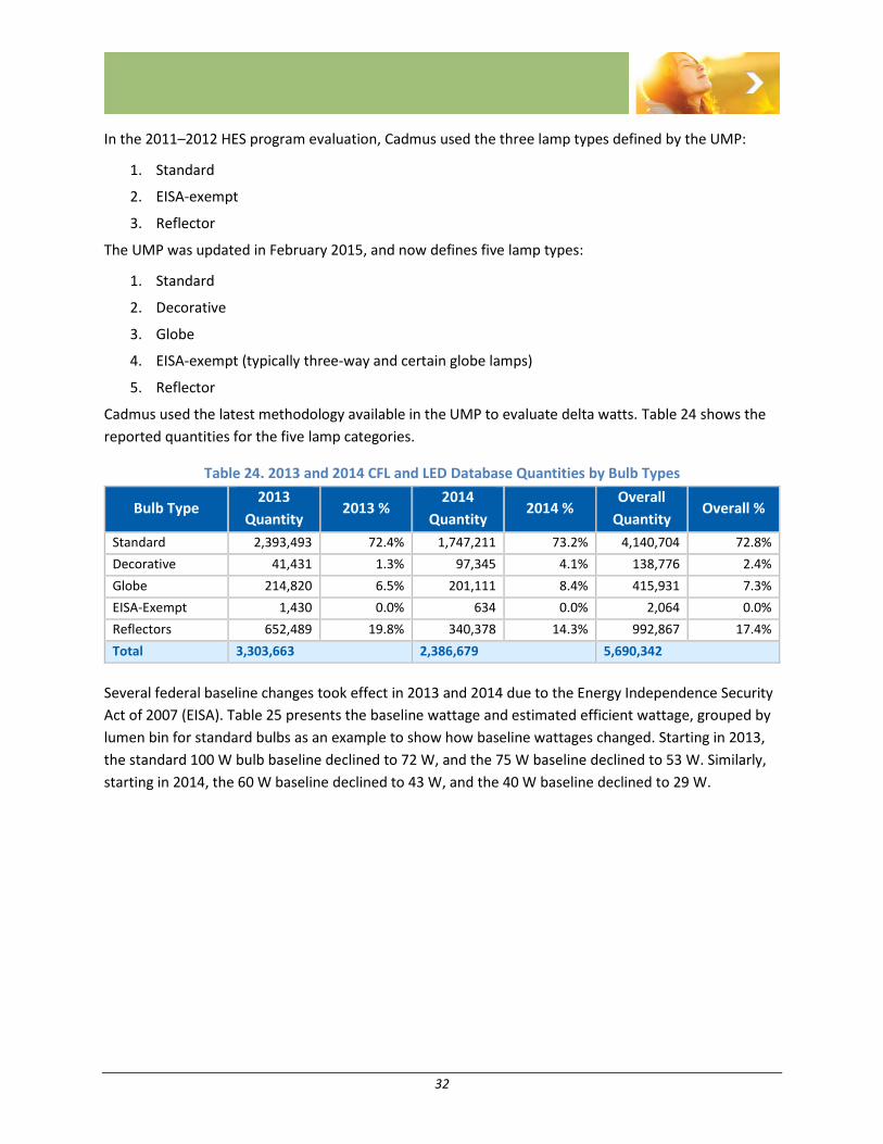
32
In the 2011–2012 HES program evaluation, Cadmus used the three lamp types defined by the UMP:
1. Standard
2. EISA-exempt
3. Reflector
The UMP was updated in February 2015, and now defines five lamp types:
1. Standard
2. Decorative
3. Globe
4. EISA-exempt (typically three-way and certain globe lamps)
5. Reflector
Cadmus used the latest methodology available in the UMP to evaluate delta watts. Table 24 shows the
reported quantities for the five lamp categories.
Table 24. 2013 and 2014 CFL and LED Database Quantities by Bulb Types
Bulb Type 2013
Quantity 2013 %
2014
Quantity 2014 %
Overall
Quantity Overall %
Standard 2,393,493 72.4% 1,747,211 73.2% 4,140,704 72.8%
Decorative 41,431 1.3% 97,345 4.1% 138,776 2.4%
Globe 214,820 6.5% 201,111 8.4% 415,931 7.3%
EISA-Exempt 1,430 0.0% 634 0.0% 2,064 0.0%
Reflectors 652,489 19.8% 340,378 14.3% 992,867 17.4%
Total 3,303,663 2,386,679 5,690,342
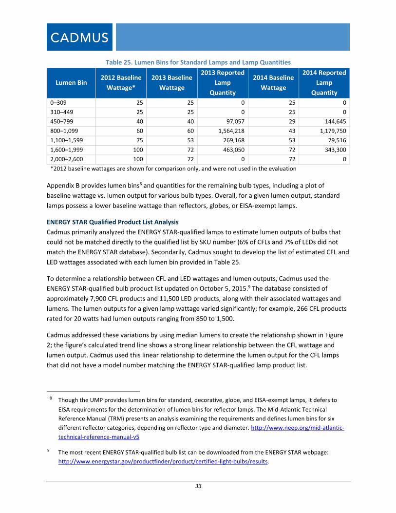
Several federal baseline changes took effect in 2013 and 2014 due to the Energy Independence Security
Act of 2007 (EISA). Table 25 presents the baseline wattage and estimated efficient wattage, grouped by
lumen bin for standard bulbs as an example to show how baseline wattages changed. Starting in 2013,
the standard 100 W bulb baseline declined to 72 W, and the 75 W baseline declined to 53 W. Similarly,
starting in 2014, the 60 W baseline declined to 43 W, and the 40 W baseline declined to 29 W.
33
Table 25. Lumen Bins for Standard Lamps and Lamp Quantities
Lumen Bin 2012 Baseline
Wattage*
2013 Baseline
Wattage
2013 Reported
Lamp
Quantity
2014 Baseline
Wattage
2014 Reported
Lamp
Quantity
0–309 25 25 0 25 0
310–449 25 25 0 25 0
450–799 40 40 97,057 29 144,645
800–1,099 60 60 1,564,218 43 1,179,750
1,100–1,599 75 53 269,168 53 79,516
1,600–1,999 100 72 463,050 72 343,300
2,000–2,600 100 72 0 72 0
*2012 baseline wattages are shown for comparison only, and were not used in the evaluation
Appendix B provides lumen bins8 and quantities for the remaining bulb types, including a plot of
baseline wattage vs. lumen output for various bulb types. Overall, for a given lumen output, standard
lamps possess a lower baseline wattage than reflectors, globes, or EISA-exempt lamps.
ENERGY STAR Qualified Product List Analysis
Cadmus primarily analyzed the ENERGY STAR-qualified lamps to estimate lumen outputs of bulbs that
could not be matched directly to the qualified list by SKU number (6% of CFLs and 7% of LEDs did not
match the ENERGY STAR database). Secondarily, Cadmus sought to develop the list of estimated CFL and
LED wattages associated with each lumen bin provided in Table 25.
To determine a relationship between CFL and LED wattages and lumen outputs, Cadmus used the
ENERGY STAR-qualified bulb product list updated on October 5, 2015.9 The database consisted of
approximately 7,900 CFL products and 11,500 LED products, along with their associated wattages and
lumens. The lumen outputs for a given lamp wattage varied significantly; for example, 266 CFL products
rated for 20 watts had lumen outputs ranging from 850 to 1,500.
Cadmus addressed these variations by using median lumens to create the relationship shown in Figure
2; the figure’s calculated trend line shows a strong linear relationship between the CFL wattage and
lumen output. Cadmus used this linear relationship to determine the lumen output for the CFL lamps
that did not have a model number matching the ENERGY STAR-qualified lamp product list.
8 Though the UMP provides lumen bins for standard, decorative, globe, and EISA-exempt lamps, it defers to
EISA requirements for the determination of lumen bins for reflector lamps. The Mid-Atlantic Technical
Reference Manual (TRM) presents an analysis examining the requirements and defines lumen bins for six
different reflector categories, depending on reflector type and diameter. http://www.neep.org/mid-atlantic-
technical-reference-manual-v5
9 The most recent ENERGY STAR-qualified bulb list can be downloaded from the ENERGY STAR webpage:
http://www.energystar.gov/productfinder/product/certified-light-bulbs/results.

34
Figure 2. Median Lumens vs. CFL Wattage for ENERGY STAR-Qualified Standard CFLs
Figure 3 shows the same chart for LED standard lamps.
Figure 3. Median Lumens vs. LED Wattage for ENERGY STAR-Qualified Standard LEDs
In total, the upstream lighting analysis employed six linear best-fit lines such as those shown above: for
LED and CFL standard, reflector, and specialty lamps. Generally, watts and lumens exhibited a stronger
relationship for CFLs than for LEDs, as shown in the above figures. Cadmus created two additional trend
lines from the ENERGY STAR database for CFL and LED fixtures. All trend lines employed are listed in
Appendix B.
Hours of Use
For 2013–2014 lighting products, Cadmus calculated an average of 1.87 HOU for CFLs and 1.92 HOU for
LEDs using analysis of covariance (ANCOVA) model coefficients, drawn from combined, multistate,
multiyear data produced by two recent CFL HOU metering studies. This model expressed average HOU
35
as a function of room type. Appendix B provides a more detailed explanation of the impact methodology
Cadmus used to estimate HOU as well as differences in the model between evaluations.
This method is consistent with those used in the 2009–2010 and 2011–2012 program year evaluations,
though the metering studies from which the data were sourced have been updated. The data used for
the 2011–2012 evaluation consisted of data for five states (Maryland, Michigan, Maine, Missouri, and
Ohio) whereas the data for the current evaluation uses data from only two (Maryland and Missouri). The
number of loggers included in the current data from just two states, however, is greater than the
number from the five states used for the previous evaluation, which allowed Cadmus to use the states
Missouri and Maryland, which are most latitudinally representative of Utah without sacrificing precision.
Lastly, these two data sources included LEDs in the logger sample, which allowed testing for differences
in HOU for LEDs and CFLs, whereas the prior data did not.
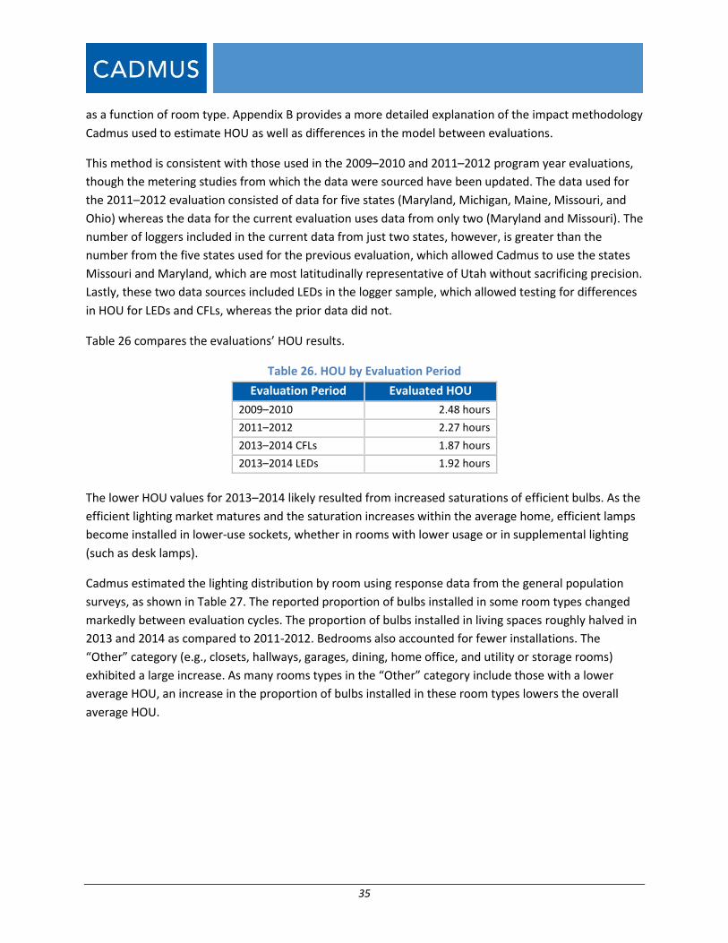
Table 26 compares the evaluations’ HOU results.
Table 26. HOU by Evaluation Period
Evaluation Period Evaluated HOU
2009–2010 2.48 hours
2011–2012 2.27 hours
2013–2014 CFLs 1.87 hours
2013–2014 LEDs 1.92 hours
The lower HOU values for 2013–2014 likely resulted from increased saturations of efficient bulbs. As the
efficient lighting market matures and the saturation increases within the average home, efficient lamps
become installed in lower-use sockets, whether in rooms with lower usage or in supplemental lighting
(such as desk lamps).
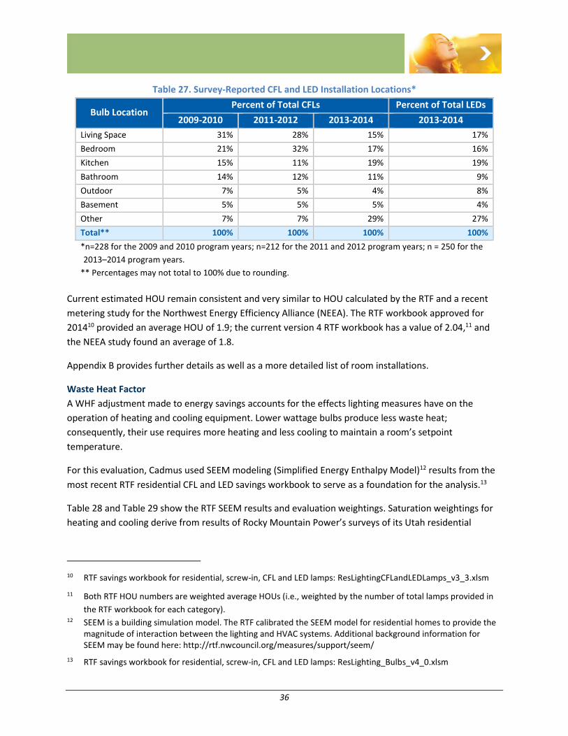
Cadmus estimated the lighting distribution by room using response data from the general population
surveys, as shown in Table 27. The reported proportion of bulbs installed in some room types changed
markedly between evaluation cycles. The proportion of bulbs installed in living spaces roughly halved in
2013 and 2014 as compared to 2011-2012. Bedrooms also accounted for fewer installations. The
“Other” category (e.g., closets, hallways, garages, dining, home office, and utility or storage rooms)
exhibited a large increase. As many rooms types in the “Other” category include those with a lower
average HOU, an increase in the proportion of bulbs installed in these room types lowers the overall
average HOU.
36
Table 27. Survey-Reported CFL and LED Installation Locations*
Bulb Location Percent of Total CFLs Percent of Total LEDs
2009-2010 2011-2012 2013-2014 2013-2014
Living Space 31% 28% 15% 17%
Bedroom 21% 32% 17% 16%
Kitchen 15% 11% 19% 19%
Bathroom 14% 12% 11% 9%
Outdoor 7% 5% 4% 8%
Basement 5% 5% 5% 4%
Other 7% 7% 29% 27%
Total** 100% 100% 100% 100%
*n=228 for the 2009 and 2010 program years; n=212 for the 2011 and 2012 program years; n = 250 for the
2013–2014 program years.
** Percentages may not total to 100% due to rounding.
Current estimated HOU remain consistent and very similar to HOU calculated by the RTF and a recent
metering study for the Northwest Energy Efficiency Alliance (NEEA). The RTF workbook approved for
201410 provided an average HOU of 1.9; the current version 4 RTF workbook has a value of 2.04,11 and
the NEEA study found an average of 1.8.
Appendix B provides further details as well as a more detailed list of room installations.
Waste Heat Factor
A WHF adjustment made to energy savings accounts for the effects lighting measures have on the
operation of heating and cooling equipment. Lower wattage bulbs produce less waste heat;
consequently, their use requires more heating and less cooling to maintain a room’s setpoint
temperature.
For this evaluation, Cadmus used SEEM modeling (Simplified Energy Enthalpy Model)12 results from the
most recent RTF residential CFL and LED savings workbook to serve as a foundation for the analysis.13
Table 28 and Table 29 show the RTF SEEM results and evaluation weightings. Saturation weightings for
heating and cooling derive from results of Rocky Mountain Power’s surveys of its Utah residential
10 RTF savings workbook for residential, screw-in, CFL and LED lamps: ResLightingCFLandLEDLamps_v3_3.xlsm
11 Both RTF HOU numbers are weighted average HOUs (i.e., weighted by the number of total lamps provided in
the RTF workbook for each category). 12 SEEM is a building simulation model. The RTF calibrated the SEEM model for residential homes to provide the
magnitude of interaction between the lighting and HVAC systems. Additional background information for SEEM may be found here: http://rtf.nwcouncil.org/measures/support/seem/
13 RTF savings workbook for residential, screw-in, CFL and LED lamps: ResLighting_Bulbs_v4_0.xlsm
37
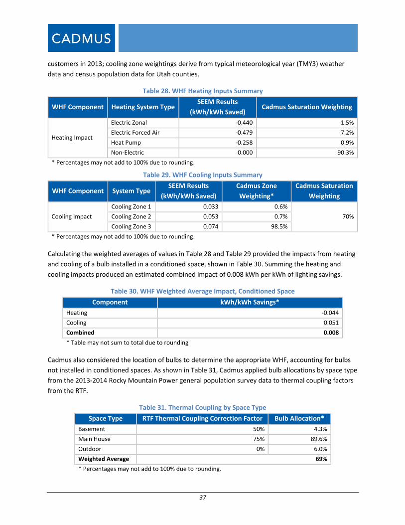
customers in 2013; cooling zone weightings derive from typical meteorological year (TMY3) weather
data and census population data for Utah counties.
Table 28. WHF Heating Inputs Summary
WHF Component Heating System Type SEEM Results
(kWh/kWh Saved) Cadmus Saturation Weighting
Heating Impact
Electric Zonal -0.440 1.5%
Electric Forced Air -0.479 7.2%
Heat Pump -0.258 0.9%
Non-Electric 0.000 90.3%
* Percentages may not add to 100% due to rounding.
Table 29. WHF Cooling Inputs Summary
WHF Component System Type SEEM Results
(kWh/kWh Saved)
Cadmus Zone
Weighting*
Cadmus Saturation
Weighting
Cooling Impact
Cooling Zone 1 0.033 0.6%
70% Cooling Zone 2 0.053 0.7%
Cooling Zone 3 0.074 98.5%
* Percentages may not add to 100% due to rounding.
Calculating the weighted averages of values in Table 28 and Table 29 provided the impacts from heating
and cooling of a bulb installed in a conditioned space, shown in Table 30. Summing the heating and
cooling impacts produced an estimated combined impact of 0.008 kWh per kWh of lighting savings.
Table 30. WHF Weighted Average Impact, Conditioned Space
Component kWh/kWh Savings*
Heating -0.044
Cooling 0.051
Combined 0.008
* Table may not sum to total due to rounding
Cadmus also considered the location of bulbs to determine the appropriate WHF, accounting for bulbs
not installed in conditioned spaces. As shown in Table 31, Cadmus applied bulb allocations by space type
from the 2013-2014 Rocky Mountain Power general population survey data to thermal coupling factors
from the RTF.
Table 31. Thermal Coupling by Space Type
Space Type RTF Thermal Coupling Correction Factor Bulb Allocation*
Basement 50% 4.3%
Main House 75% 89.6%
Outdoor 0% 6.0%
Weighted Average 69%
* Percentages may not add to 100% due to rounding.
38
Multiplying the combined impact from Table 30 with the weighted thermal coupling in Table 31 and
adding 1 provided the final WHF shown in Table 32.
Table 32. Utah CFL and LED Bulb WHF, Average Installation Location
Fuel Value Units
Electric 1.005* kWh/kWh Saved
*Final WHF value does not compute exactly from reported variables due to rounding.
Cross-Sector Sales
During the intercept surveys, Cadmus collected data on the intended installation locations of efficient
bulbs purchased at retailer stores. Recent data collected in several jurisdictions around the country,
reveal that many program bulbs are installed in commercial settings. Bulbs installed in commercial
spaces produce more first-year savings than bulbs installed in a residential space because commercial
locations typically have a higher daily use of bulbs than residential locations (i.e., higher HOU).
Percentages of bulbs purchased from retail stores and installed in commercial buildings are called cross-
sector sales.
Of all bulbs purchased at participating retailers, Cadmus estimated that 3.9% of efficient bulbs
ultimately would be installed in commercial applications. Cadmus did not include this adjustment in the
gross savings calculation. Other jurisdictions around the country have increasingly accommodated cross-
sector sales factors in calculating lighting savings; such an adjustment would require an update to
savings calculations from those presented in this report. Appendix B contains further details regarding
cross-sector sales methodology and results.
CFL and LED Bulbs Total Savings
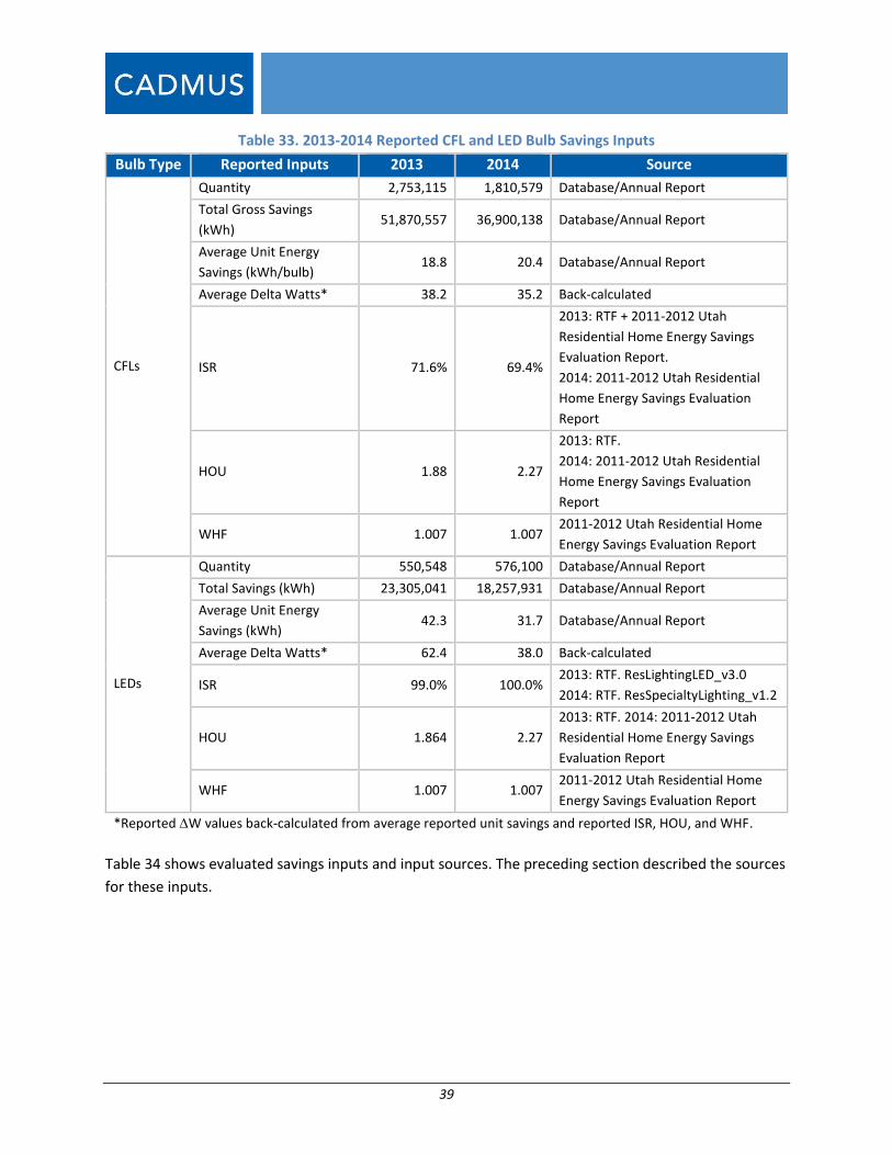
Table 33 shows reported savings inputs and input sources. Cadmus determined these inputs using
assumptions provided by Rocky Mountain Power and information drawn from the tracking database.
Reported values for ISR, HOU, and WHF were sourced directly from the assumption workbooks
provided. Reported values for UES were calculated from the tracking database, and average values for
delta watts were back-calculated from the reported savings using the ISR, HOU, and WHF assumptions
from the UES workbooks provided.
39
Table 33. 2013-2014 Reported CFL and LED Bulb Savings Inputs
Bulb Type Reported Inputs 2013 2014 Source
CFLs
Quantity 2,753,115 1,810,579 Database/Annual Report
Total Gross Savings
(kWh) 51,870,557 36,900,138 Database/Annual Report
Average Unit Energy
Savings (kWh/bulb) 18.8 20.4 Database/Annual Report
Average Delta Watts* 38.2 35.2 Back-calculated
ISR 71.6% 69.4%
2013: RTF + 2011-2012 Utah
Residential Home Energy Savings
Evaluation Report.
2014: 2011-2012 Utah Residential
Home Energy Savings Evaluation
Report
HOU 1.88 2.27
2013: RTF.
2014: 2011-2012 Utah Residential
Home Energy Savings Evaluation
Report
WHF 1.007 1.007 2011-2012 Utah Residential Home
Energy Savings Evaluation Report
LEDs
Quantity 550,548 576,100 Database/Annual Report
Total Savings (kWh) 23,305,041 18,257,931 Database/Annual Report
Average Unit Energy
Savings (kWh) 42.3 31.7 Database/Annual Report
Average Delta Watts* 62.4 38.0 Back-calculated
ISR 99.0% 100.0% 2013: RTF. ResLightingLED_v3.0
2014: RTF. ResSpecialtyLighting_v1.2
HOU 1.864 2.27
2013: RTF. 2014: 2011-2012 Utah
Residential Home Energy Savings
Evaluation Report
WHF 1.007 1.007 2011-2012 Utah Residential Home
Energy Savings Evaluation Report
*Reported W values back-calculated from average reported unit savings and reported ISR, HOU, and WHF.
Table 34 shows evaluated savings inputs and input sources. The preceding section described the sources
for these inputs.
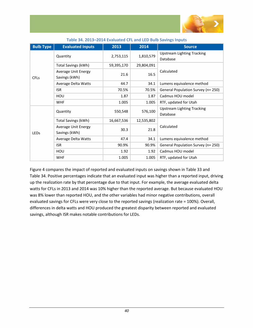
40
Table 34. 2013–2014 Evaluated CFL and LED Bulb Savings Inputs
Bulb Type Evaluated Inputs 2013 2014 Source
CFLs
Quantity 2,753,115 1,810,579 Upstream Lighting Tracking
Database
Total Savings (kWh) 59,395,170 29,804,091
Calculated Average Unit Energy
Savings (kWh) 21.6 16.5
Average Delta Watts 44.7 34.1 Lumens equivalence method
ISR 70.5% 70.5% General Population Survey (n= 250)
HOU 1.87 1.87 Cadmus HOU model
WHF 1.005 1.005 RTF, updated for Utah
LEDs
Quantity 550,548 576,100 Upstream Lighting Tracking
Database
Total Savings (kWh) 16,667,536 12,535,802
Calculated Average Unit Energy
Savings (kWh) 30.3 21.8
Average Delta Watts 47.4 34.1 Lumens equivalence method
ISR 90.9% 90.9% General Population Survey (n= 250)
HOU 1.92 1.92 Cadmus HOU model
WHF 1.005 1.005 RTF, updated for Utah
Figure 4 compares the impact of reported and evaluated inputs on savings shown in Table 33 and
Table 34. Positive percentages indicate that an evaluated input was higher than a reported input, driving
up the realization rate by that percentage due to that input. For example, the average evaluated delta
watts for CFLs in 2013 and 2014 was 10% higher than the reported average. But because evaluated HOU
was 8% lower than reported HOU, and the other variables had minor negative contributions, overall
evaluated savings for CFLs were very close to the reported savings (realization rate = 100%). Overall,
differences in delta watts and HOU produced the greatest disparity between reported and evaluated
savings, although ISR makes notable contributions for LEDs.
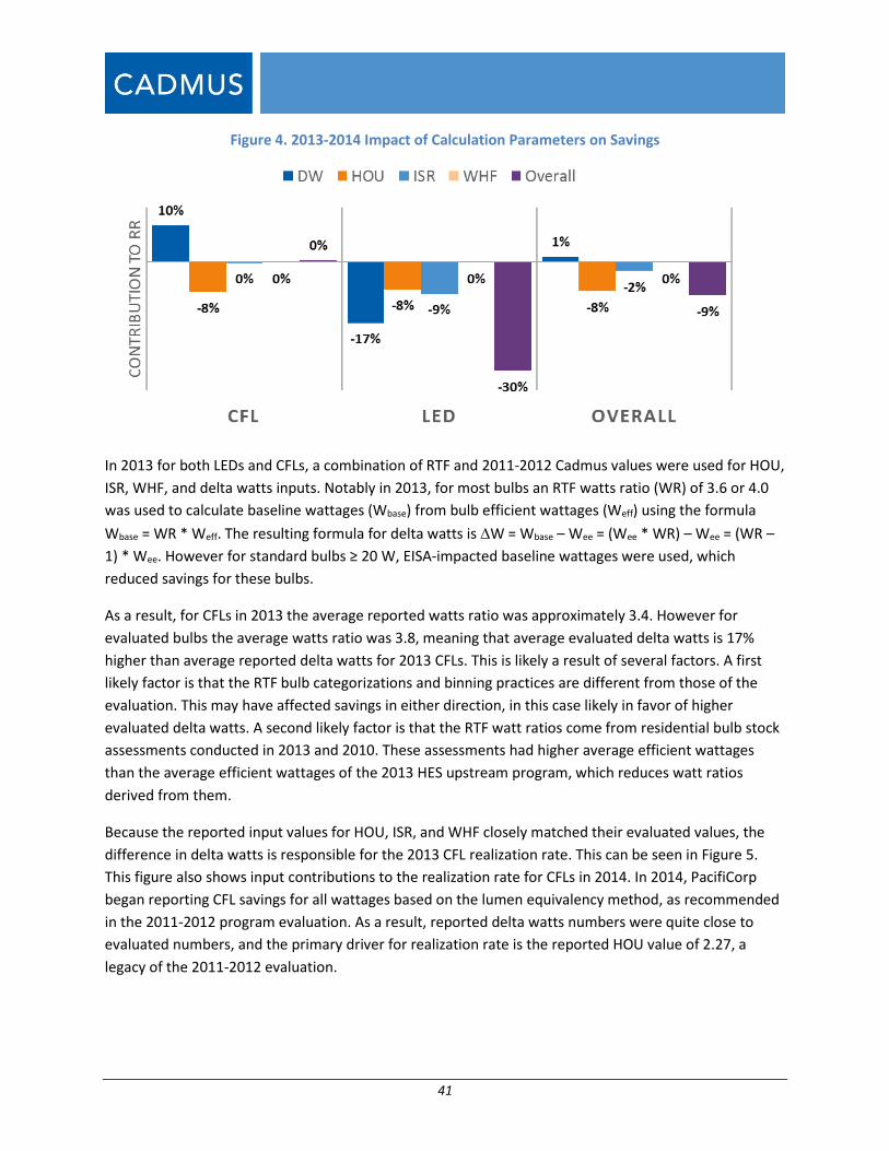
41
Figure 4. 2013-2014 Impact of Calculation Parameters on Savings
In 2013 for both LEDs and CFLs, a combination of RTF and 2011-2012 Cadmus values were used for HOU,
ISR, WHF, and delta watts inputs. Notably in 2013, for most bulbs an RTF watts ratio (WR) of 3.6 or 4.0
was used to calculate baseline wattages (Wbase) from bulb efficient wattages (Weff) using the formula
Wbase = WR * Weff. The resulting formula for delta watts is W = Wbase – Wee = (Wee * WR) – Wee = (WR –
1) * Wee. However for standard bulbs ≥ 20 W, EISA-impacted baseline wattages were used, which
reduced savings for these bulbs.
As a result, for CFLs in 2013 the average reported watts ratio was approximately 3.4. However for
evaluated bulbs the average watts ratio was 3.8, meaning that average evaluated delta watts is 17%
higher than average reported delta watts for 2013 CFLs. This is likely a result of several factors. A first
likely factor is that the RTF bulb categorizations and binning practices are different from those of the
evaluation. This may have affected savings in either direction, in this case likely in favor of higher
evaluated delta watts. A second likely factor is that the RTF watt ratios come from residential bulb stock
assessments conducted in 2013 and 2010. These assessments had higher average efficient wattages
than the average efficient wattages of the 2013 HES upstream program, which reduces watt ratios
derived from them.
Because the reported input values for HOU, ISR, and WHF closely matched their evaluated values, the
difference in delta watts is responsible for the 2013 CFL realization rate. This can be seen in Figure 5.
This figure also shows input contributions to the realization rate for CFLs in 2014. In 2014, PacifiCorp
began reporting CFL savings for all wattages based on the lumen equivalency method, as recommended
in the 2011-2012 program evaluation. As a result, reported delta watts numbers were quite close to
evaluated numbers, and the primary driver for realization rate is the reported HOU value of 2.27, a
legacy of the 2011-2012 evaluation.
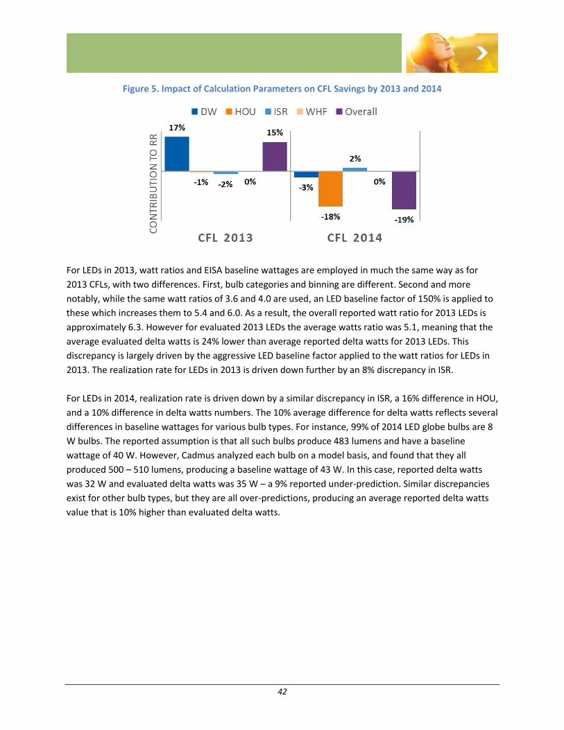
42
Figure 5. Impact of Calculation Parameters on CFL Savings by 2013 and 2014
For LEDs in 2013, watt ratios and EISA baseline wattages are employed in much the same way as for
2013 CFLs, with two differences. First, bulb categories and binning are different. Second and more
notably, while the same watt ratios of 3.6 and 4.0 are used, an LED baseline factor of 150% is applied to
these which increases them to 5.4 and 6.0. As a result, the overall reported watt ratio for 2013 LEDs is
approximately 6.3. However for evaluated 2013 LEDs the average watts ratio was 5.1, meaning that the
average evaluated delta watts is 24% lower than average reported delta watts for 2013 LEDs. This
discrepancy is largely driven by the aggressive LED baseline factor applied to the watt ratios for LEDs in
2013. The realization rate for LEDs in 2013 is driven down further by an 8% discrepancy in ISR.
For LEDs in 2014, realization rate is driven down by a similar discrepancy in ISR, a 16% difference in HOU,
and a 10% difference in delta watts numbers. The 10% average difference for delta watts reflects several
differences in baseline wattages for various bulb types. For instance, 99% of 2014 LED globe bulbs are 8
W bulbs. The reported assumption is that all such bulbs produce 483 lumens and have a baseline
wattage of 40 W. However, Cadmus analyzed each bulb on a model basis, and found that they all
produced 500 – 510 lumens, producing a baseline wattage of 43 W. In this case, reported delta watts
was 32 W and evaluated delta watts was 35 W – a 9% reported under-prediction. Similar discrepancies
exist for other bulb types, but they are all over-predictions, producing an average reported delta watts
value that is 10% higher than evaluated delta watts.
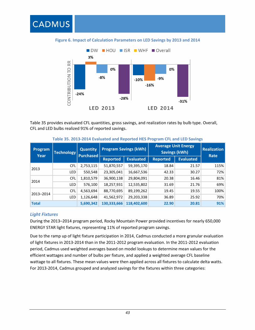
43
Figure 6. Impact of Calculation Parameters on LED Savings by 2013 and 2014
Table 35 provides evaluated CFL quantities, gross savings, and realization rates by bulb type. Overall, CFL and LED bulbs realized 91% of reported savings.
Table 35. 2013-2014 Evaluated and Reported HES Program CFL and LED Savings
Program
Year Technology
Quantity
Purchased
Program Savings (kWh) Average Unit Energy
Savings (kWh) Realization
Rate Reported Evaluated Reported Evaluated
2013 CFL 2,753,115 51,870,557 59,395,170 18.84 21.57 115%
LED 550,548 23,305,041 16,667,536 42.33 30.27 72%
2014 CFL 1,810,579 36,900,138 29,804,091 20.38 16.46 81%
LED 576,100 18,257,931 12,535,802 31.69 21.76 69%
2013–2014 CFL 4,563,694 88,770,695 89,199,262 19.45 19.55 100%
LED 1,126,648 41,562,972 29,203,338 36.89 25.92 70%
Total 5,690,342 130,333,666 118,402,600 22.90 20.81 91%
Light Fixtures
During the 2013–2014 program period, Rocky Mountain Power provided incentives for nearly 650,000
ENERGY STAR light fixtures, representing 11% of reported program savings.
Due to the ramp up of light fixture participation in 2014, Cadmus conducted a more granular evaluation
of light fixtures in 2013-2014 than in the 2011-2012 program evaluation. In the 2011-2012 evaluation
period, Cadmus used weighted averages based on model lookups to determine mean values for the
efficient wattages and number of bulbs per fixture, and applied a weighted average CFL baseline
wattage to all fixtures. These mean values were then applied across all fixtures to calculate delta watts.
For 2013-2014, Cadmus grouped and analyzed savings for the fixtures within three categories:
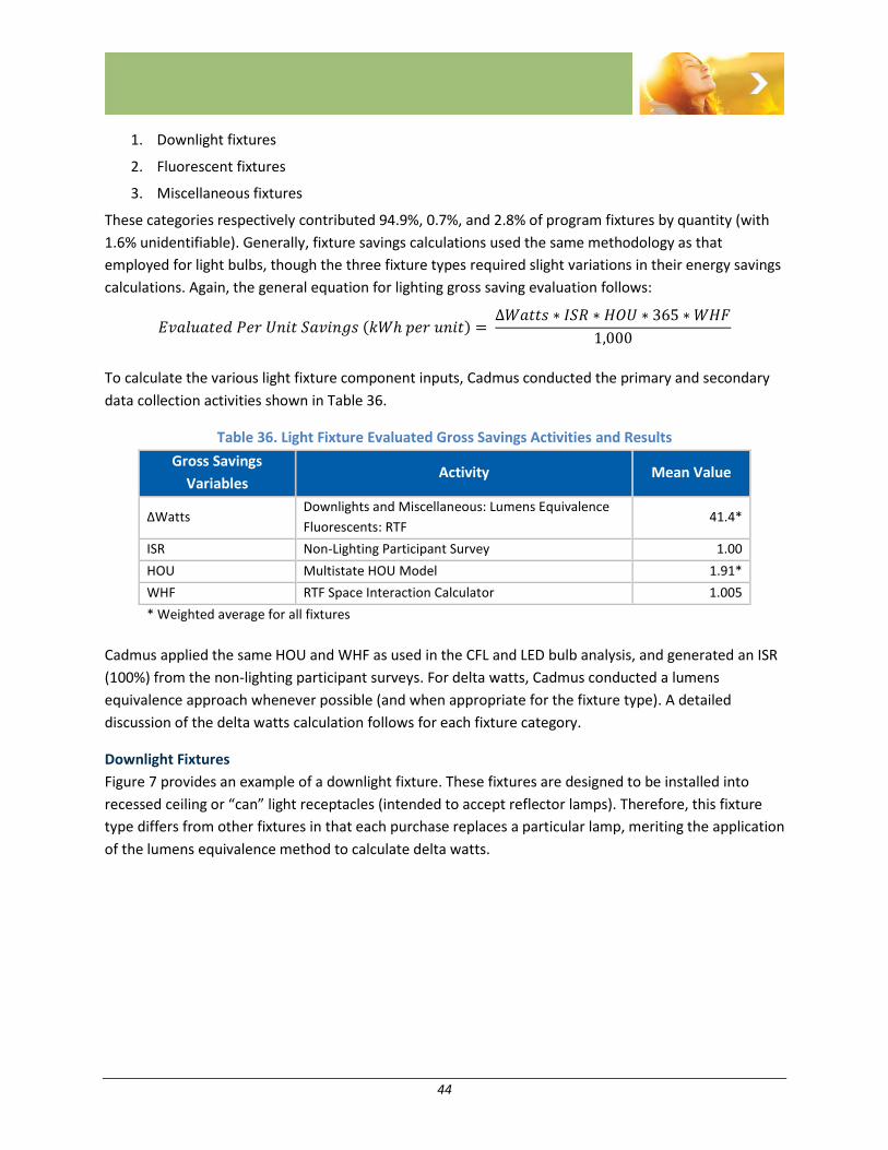
44
1. Downlight fixtures
2. Fluorescent fixtures
3. Miscellaneous fixtures
These categories respectively contributed 94.9%, 0.7%, and 2.8% of program fixtures by quantity (with
1.6% unidentifiable). Generally, fixture savings calculations used the same methodology as that
employed for light bulbs, though the three fixture types required slight variations in their energy savings
calculations. Again, the general equation for lighting gross saving evaluation follows:
𝐸𝑣𝑎𝑙𝑢𝑎𝑡𝑒𝑑 𝑃𝑒𝑟 𝑈𝑛𝑖𝑡 𝑆𝑎𝑣𝑖𝑛𝑔𝑠 (𝑘𝑊ℎ 𝑝𝑒𝑟 𝑢𝑛𝑖𝑡) = ∆𝑊𝑎𝑡𝑡𝑠 ∗ 𝐼𝑆𝑅 ∗ 𝐻𝑂𝑈 ∗ 365 ∗ 𝑊𝐻𝐹
1,000
To calculate the various light fixture component inputs, Cadmus conducted the primary and secondary
data collection activities shown in Table 36.
Table 36. Light Fixture Evaluated Gross Savings Activities and Results
Gross Savings
Variables Activity Mean Value
ΔWatts Downlights and Miscellaneous: Lumens Equivalence
Fluorescents: RTF 41.4*
ISR Non-Lighting Participant Survey 1.00
HOU Multistate HOU Model 1.91*
WHF RTF Space Interaction Calculator 1.005
* Weighted average for all fixtures
Cadmus applied the same HOU and WHF as used in the CFL and LED bulb analysis, and generated an ISR
(100%) from the non-lighting participant surveys. For delta watts, Cadmus conducted a lumens
equivalence approach whenever possible (and when appropriate for the fixture type). A detailed
discussion of the delta watts calculation follows for each fixture category.
Downlight Fixtures
Figure 7 provides an example of a downlight fixture. These fixtures are designed to be installed into
recessed ceiling or “can” light receptacles (intended to accept reflector lamps). Therefore, this fixture
type differs from other fixtures in that each purchase replaces a particular lamp, meriting the application
of the lumens equivalence method to calculate delta watts.

45
Figure 7. Example of a Donwlight Fixture
The types of lamps typically replaced by LED downlight fixtures must be determined in order to calculate
baseline wattages for LED downlights. While recessed ceiling fixtures are typically designed to
accommodate reflector lamps that point light down to maximize the light output, sometimes other lamp
types may be installed. Using data compiled from household lighting inventories conducted in four other
jurisdictions across the United States, Cadmus calculated a weighted baseline wattage for LED downlight
fixtures that accounts for the mix of bulb types typically installed in recessed ceiling receptacles.
To do this, Cadmus first calculated an average set of reflector lumen bins and baseline wattages that
account for the six different types of reflector lamps. The lumen bins and baseline wattages for each
reflector type were weighted by their quantities in the upstream lighting database, which is the closest
source of granular sales data available.
This set of average reflector baseline wattages and lumen bins was then combined with the lumen bins
and baseline wattages for other lamp types, weighted by saturation of bulb types typically installed in
recessed ceiling receptacles as determined by the four lighting inventories. The inventories collected
data on the type of bulb installed in every fixture in over 200 homes. Using this data, Cadmus
determined saturation levels of various lamp types typically installed in recessed ceiling receptacles.
Results are presented in Table 37, showing that 85.6% of lamps installed in ceiling receptacles were
reflector lamps and 13.5% were standard lamps, with the other categories comprising the rest. These
saturation values were used to create an average set of lumen bins and baseline wattages for recessed
ceiling receptacles, for both 2013 and 2014. Plots of the weighted reflector and final recessed can lumen
bins and baseline wattages can be seen in Appendix B. Like reflector baseline wattages in general, the
recessed can baseline wattage values are generally higher than those for standard lamps.

46
Table 37. Lamp Type Saturation in Recessed Ceiling Receptacles
Lamp Type Southwestern
Utility
Central
Utility
Midwest
Utility
Mid-Atlantic
Utility Combined
Standard 11.70% 17.60% 13.20% 12.70% 13.52%
Globe 0.60% 0.50% 0.00% 0.90% 0.60%
Reflector 87.70% 81.90% 86.00% 86.00% 85.57%
Decorative 0.00% 0.00% 0.30% 0.40% 0.22%
EISA-Exempt 0.00% 0.00% 0.50% 0.00% 0.09%
Total Bulbs 473 431 393 928 2225
Total Households 38 46 68 65 217
Fluorescent Fixtures
The lumens equivalency method cannot be applied to fluorescent lamps (0.7% of fixtures). Instead, a
single delta watts value was applied for all fluorescent lamps in the database. While the database
includes some circline and other types of fluorescent lights, the majority (> 80%) of fluorescent lamps
are two-lamp T8 fluorescents.
Cadmus applied the delta watts value from the RTF for fluorescent fixtures. The High-Performance T8
Lamps Workbook14 (Version 1.1) provides a delta watts value of 42 W for 4-foot, two-lamp T8 fixtures
installed in kitchens and 43 W value for the same fixtures installed in garages. As the installation
locations for these fixtures remains unknown, Cadmus applied a 42.5 delta watts value for all
fluorescent lamp fixtures in the database. Cadmus applied CFL values for HOU and WHF.
Miscellaneous Fixtures
Just under 3% of fixtures sold could not be classified as downlights or fluorescent lights (e.g., single- and
multi-bulb sconce lights, motion sensors, track lighting). Roughly one third were single-lamp CFL fixtures,
one third were two-lamp CFL fixtures, and one third were LED fixtures of various types. Cadmus applied
the lumens equivalence approach to evaluate these fixtures.
Unknown Fixtures
The database included 1.6% of fixtures falling within unknown categories. Of these, 94% had no model
numbers in the database. The remainder could not be matched to the ENERGY STAR database.
Consequently, Cadmus applied the weighted average UES for the downlight, fluorescent, and
miscellaneous fixture categories.
Lighting Fixture Findings
In 2013–2014, the HES program provided incentives for 646,893 light fixtures. Table 38 provides lamp
quantities, savings, and realization rates by fixture type for 2013–2014.
14 http://rtf.nwcouncil.org/measures/res/ResLightingHPT8Lamps_v1_1.xlsm
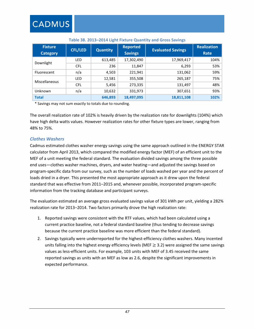
47
Table 38. 2013–2014 Light Fixture Quantity and Gross Savings
Fixture
Category CFL/LED Quantity
Reported
Savings Evaluated Savings
Realization
Rate
Downlight LED 613,485 17,302,490 17,969,417 104%
CFL 236 11,847 6,293 53%
Fluorescent n/a 4,503 221,941 131,062 59%
Miscellaneous LED 12,581 355,508 265,187 75%
CFL 5,456 273,335 131,497 48%
Unknown n/a 10,632 331,973 307,651 93%
Total 646,893 18,497,095 18,811,108 102%
* Savings may not sum exactly to totals due to rounding.
The overall realization rate of 102% is heavily driven by the realization rate for downlights (104%) which
have high delta watts values. However realization rates for other fixture types are lower, ranging from
48% to 75%.
Clothes Washers
Cadmus estimated clothes washer energy savings using the same approach outlined in the ENERGY STAR
calculator from April 2013, which compared the modified energy factor (MEF) of an efficient unit to the
MEF of a unit meeting the federal standard. The evaluation divided savings among the three possible
end uses—clothes washer machines, dryers, and water heating—and adjusted the savings based on
program-specific data from our survey, such as the number of loads washed per year and the percent of
loads dried in a dryer. This presented the most appropriate approach as it drew upon the federal
standard that was effective from 2011–2015 and, whenever possible, incorporated program-specific
information from the tracking database and participant surveys.
The evaluation estimated an average gross evaluated savings value of 301 kWh per unit, yielding a 282%
realization rate for 2013–2014. Two factors primarily drove the high realization rate:
1. Reported savings were consistent with the RTF values, which had been calculated using a
current practice baseline, not a federal standard baseline (thus tending to decrease savings
because the current practice baseline was more efficient than the federal standard).
2. Savings typically were underreported for the highest-efficiency clothes washers. Many incented
units falling into the highest energy efficiency levels (MEF ≥ 3.2) were assigned the same savings
values as less-efficient units. For example, 103 units with MEF of 3.45 received the same
reported savings as units with an MEF as low as 2.6, despite the significant improvements in
expected performance.
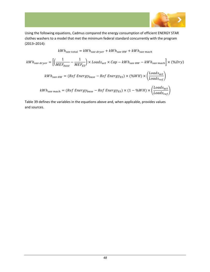
48
Using the following equations, Cadmus compared the energy consumption of efficient ENERGY STAR
clothes washers to a model that met the minimum federal standard concurrently with the program
(2013–2014):
𝑘𝑊ℎ𝑠𝑎𝑣 𝑡𝑜𝑡𝑎𝑙 = 𝑘𝑊ℎ𝑠𝑎𝑣 𝑑𝑟𝑦𝑒𝑟 + 𝑘𝑊ℎ𝑠𝑎𝑣 𝐻𝑊 + 𝑘𝑊ℎ𝑠𝑎𝑣 𝑚𝑎𝑐ℎ
𝑘𝑊ℎ𝑠𝑎𝑣 𝑑𝑟𝑦𝑒𝑟 = [(1
𝑀𝐸𝐹𝑏𝑎𝑠𝑒−
1
𝑀𝐸𝐹𝐸𝑆) × 𝐿𝑜𝑎𝑑𝑠𝑎𝑐𝑡 × 𝐶𝑎𝑝 − 𝑘𝑊ℎ𝑠𝑎𝑣 𝐻𝑊 − 𝑘𝑊ℎ𝑠𝑎𝑣 𝑚𝑎𝑐ℎ] × (%𝐷𝑟𝑦)
𝑘𝑊ℎ𝑠𝑎𝑣 𝐻𝑊 = (𝑅𝑒𝑓 𝐸𝑛𝑒𝑟𝑔𝑦𝑏𝑎𝑠𝑒 − 𝑅𝑒𝑓 𝐸𝑛𝑒𝑟𝑔𝑦𝐸𝑆) × (%𝑊𝐻) × (𝐿𝑜𝑎𝑑𝑠𝑎𝑐𝑡
𝐿𝑜𝑎𝑑𝑠𝑟𝑒𝑓)
𝑘𝑊ℎ𝑠𝑎𝑣 𝑚𝑎𝑐ℎ = (𝑅𝑒𝑓 𝐸𝑛𝑒𝑟𝑔𝑦𝑏𝑎𝑠𝑒 − 𝑅𝑒𝑓 𝐸𝑛𝑒𝑟𝑔𝑦𝐸𝑆) × (1 − %𝑊𝐻) × (𝐿𝑜𝑎𝑑𝑠𝑎𝑐𝑡
𝐿𝑜𝑎𝑑𝑠𝑟𝑒𝑓)
Table 39 defines the variables in the equations above and, when applicable, provides values
and sources.
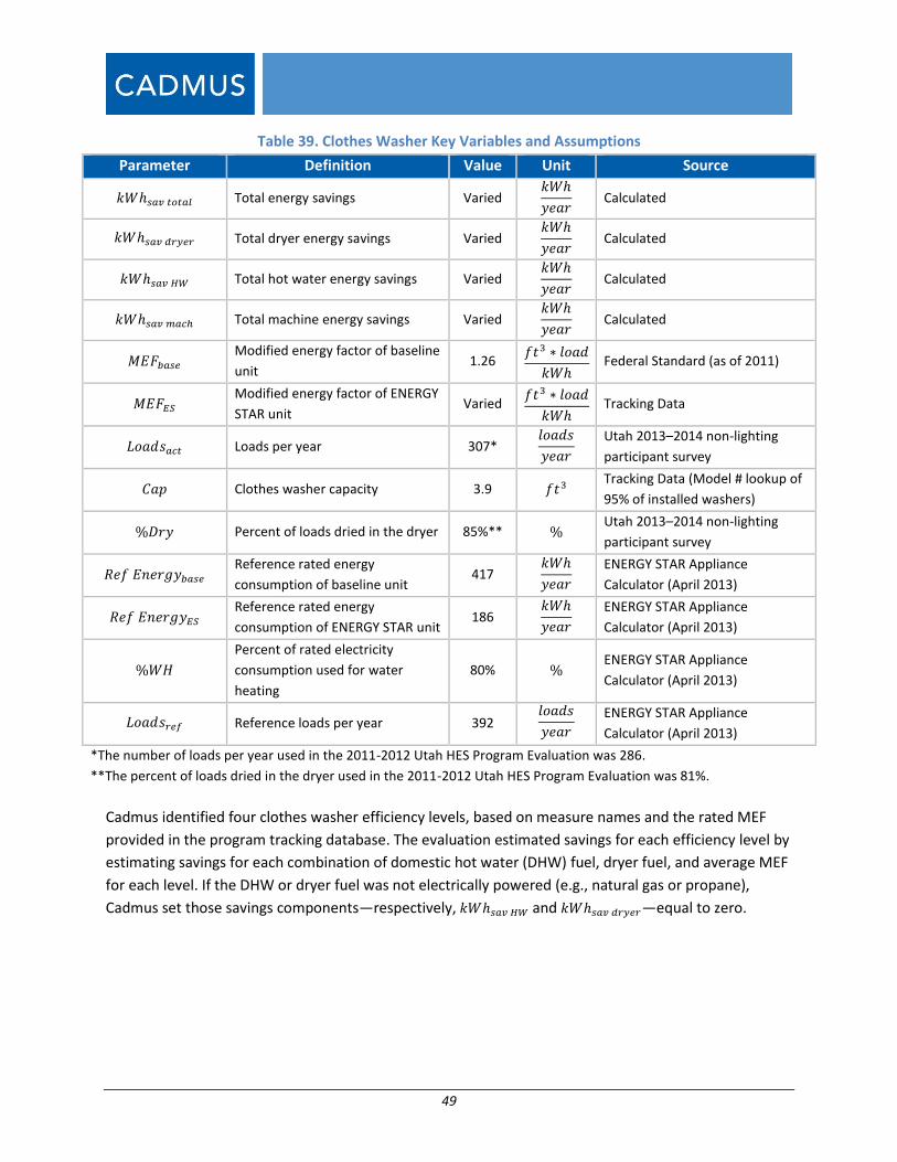
49
Table 39. Clothes Washer Key Variables and Assumptions
Parameter Definition Value Unit Source
𝑘𝑊ℎ𝑠𝑎𝑣 𝑡𝑜𝑡𝑎𝑙 Total energy savings Varied 𝑘𝑊ℎ
𝑦𝑒𝑎𝑟 Calculated
𝑘𝑊ℎ𝑠𝑎𝑣 𝑑𝑟𝑦𝑒𝑟 Total dryer energy savings Varied 𝑘𝑊ℎ
𝑦𝑒𝑎𝑟 Calculated
𝑘𝑊ℎ𝑠𝑎𝑣 𝐻𝑊 Total hot water energy savings Varied 𝑘𝑊ℎ
𝑦𝑒𝑎𝑟 Calculated
𝑘𝑊ℎ𝑠𝑎𝑣 𝑚𝑎𝑐ℎ Total machine energy savings Varied 𝑘𝑊ℎ
𝑦𝑒𝑎𝑟 Calculated
𝑀𝐸𝐹𝑏𝑎𝑠𝑒 Modified energy factor of baseline
unit 1.26
𝑓𝑡3 ∗ 𝑙𝑜𝑎𝑑
𝑘𝑊ℎ Federal Standard (as of 2011)
𝑀𝐸𝐹𝐸𝑆 Modified energy factor of ENERGY
STAR unit Varied
𝑓𝑡3 ∗ 𝑙𝑜𝑎𝑑
𝑘𝑊ℎ Tracking Data
𝐿𝑜𝑎𝑑𝑠𝑎𝑐𝑡 Loads per year 307* 𝑙𝑜𝑎𝑑𝑠
𝑦𝑒𝑎𝑟
Utah 2013–2014 non-lighting
participant survey
𝐶𝑎𝑝 Clothes washer capacity 3.9 𝑓𝑡3 Tracking Data (Model # lookup of
95% of installed washers)
%𝐷𝑟𝑦 Percent of loads dried in the dryer 85%** % Utah 2013–2014 non-lighting
participant survey
𝑅𝑒𝑓 𝐸𝑛𝑒𝑟𝑔𝑦𝑏𝑎𝑠𝑒 Reference rated energy
consumption of baseline unit 417
𝑘𝑊ℎ
𝑦𝑒𝑎𝑟
ENERGY STAR Appliance
Calculator (April 2013)
𝑅𝑒𝑓 𝐸𝑛𝑒𝑟𝑔𝑦𝐸𝑆 Reference rated energy
consumption of ENERGY STAR unit 186
𝑘𝑊ℎ
𝑦𝑒𝑎𝑟
ENERGY STAR Appliance
Calculator (April 2013)
%𝑊𝐻
Percent of rated electricity
consumption used for water
heating
80% % ENERGY STAR Appliance
Calculator (April 2013)
𝐿𝑜𝑎𝑑𝑠𝑟𝑒𝑓 Reference loads per year 392 𝑙𝑜𝑎𝑑𝑠
𝑦𝑒𝑎𝑟
ENERGY STAR Appliance
Calculator (April 2013)
*The number of loads per year used in the 2011-2012 Utah HES Program Evaluation was 286.
**The percent of loads dried in the dryer used in the 2011-2012 Utah HES Program Evaluation was 81%.
Cadmus identified four clothes washer efficiency levels, based on measure names and the rated MEF
provided in the program tracking database. The evaluation estimated savings for each efficiency level by
estimating savings for each combination of domestic hot water (DHW) fuel, dryer fuel, and average MEF
for each level. If the DHW or dryer fuel was not electrically powered (e.g., natural gas or propane),
Cadmus set those savings components—respectively, 𝑘𝑊ℎ𝑠𝑎𝑣 𝐻𝑊 and 𝑘𝑊ℎ𝑠𝑎𝑣 𝑑𝑟𝑦𝑒𝑟—equal to zero.
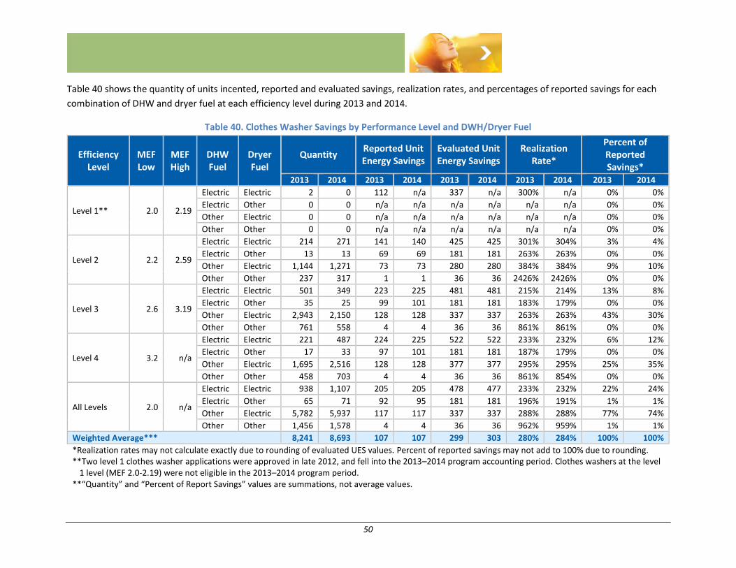
50
Table 40 shows the quantity of units incented, reported and evaluated savings, realization rates, and percentages of reported savings for each
combination of DHW and dryer fuel at each efficiency level during 2013 and 2014.
Table 40. Clothes Washer Savings by Performance Level and DWH/Dryer Fuel
Efficiency Level
MEF Low
MEF High
DHW Fuel
Dryer Fuel
Quantity Reported Unit Energy Savings
Evaluated Unit Energy Savings
Realization Rate*
Percent of Reported Savings*
2013 2014 2013 2014 2013 2014 2013 2014 2013 2014
Level 1** 2.0 2.19
Electric Electric 2 0 112 n/a 337 n/a 300% n/a 0% 0%
Electric Other 0 0 n/a n/a n/a n/a n/a n/a 0% 0%
Other Electric 0 0 n/a n/a n/a n/a n/a n/a 0% 0%
Other Other 0 0 n/a n/a n/a n/a n/a n/a 0% 0%
Level 2 2.2 2.59
Electric Electric 214 271 141 140 425 425 301% 304% 3% 4%
Electric Other 13 13 69 69 181 181 263% 263% 0% 0%
Other Electric 1,144 1,271 73 73 280 280 384% 384% 9% 10%
Other Other 237 317 1 1 36 36 2426% 2426% 0% 0%
Level 3 2.6 3.19
Electric Electric 501 349 223 225 481 481 215% 214% 13% 8%
Electric Other 35 25 99 101 181 181 183% 179% 0% 0%
Other Electric 2,943 2,150 128 128 337 337 263% 263% 43% 30%
Other Other 761 558 4 4 36 36 861% 861% 0% 0%
Level 4 3.2 n/a
Electric Electric 221 487 224 225 522 522 233% 232% 6% 12%
Electric Other 17 33 97 101 181 181 187% 179% 0% 0%
Other Electric 1,695 2,516 128 128 377 377 295% 295% 25% 35%
Other Other 458 703 4 4 36 36 861% 854% 0% 0%
All Levels
2.0 n/a
Electric Electric 938 1,107 205 205 478 477 233% 232% 22% 24%
Electric Other 65 71 92 95 181 181 196% 191% 1% 1%
Other Electric 5,782 5,937 117 117 337 337 288% 288% 77% 74%
Other Other 1,456 1,578 4 4 36 36 962% 959% 1% 1%
Weighted Average*** 8,241 8,693 107 107 299 303 280% 284% 100% 100%
*Realization rates may not calculate exactly due to rounding of evaluated UES values. Percent of reported savings may not add to 100% due to rounding. **Two level 1 clothes washer applications were approved in late 2012, and fell into the 2013–2014 program accounting period. Clothes washers at the level
1 level (MEF 2.0-2.19) were not eligible in the 2013–2014 program period. **“Quantity” and “Percent of Report Savings” values are summations, not average values.
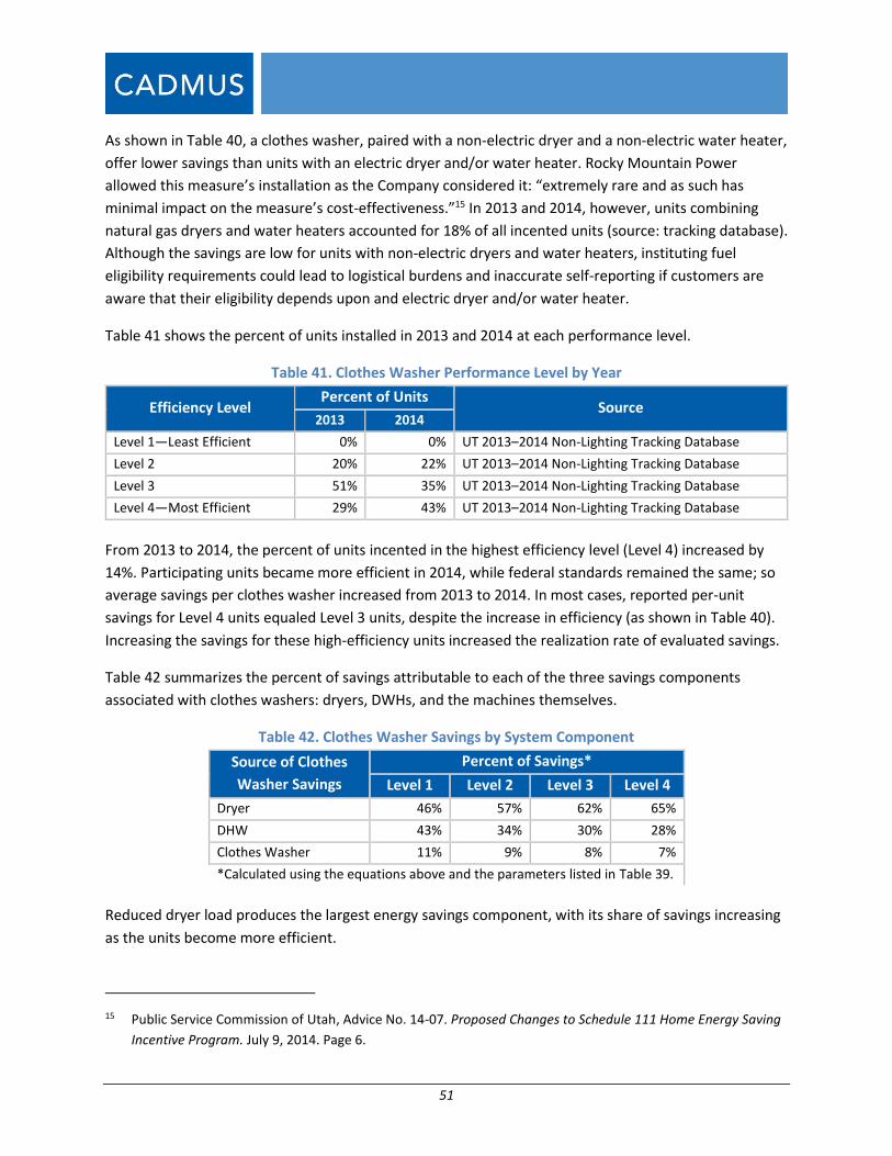
51
As shown in Table 40, a clothes washer, paired with a non-electric dryer and a non-electric water heater,
offer lower savings than units with an electric dryer and/or water heater. Rocky Mountain Power
allowed this measure’s installation as the Company considered it: “extremely rare and as such has
minimal impact on the measure’s cost-effectiveness.”15 In 2013 and 2014, however, units combining
natural gas dryers and water heaters accounted for 18% of all incented units (source: tracking database).
Although the savings are low for units with non-electric dryers and water heaters, instituting fuel
eligibility requirements could lead to logistical burdens and inaccurate self-reporting if customers are
aware that their eligibility depends upon and electric dryer and/or water heater.
Table 41 shows the percent of units installed in 2013 and 2014 at each performance level.
Table 41. Clothes Washer Performance Level by Year
Efficiency Level Percent of Units
Source 2013 2014
Level 1—Least Efficient 0% 0% UT 2013–2014 Non-Lighting Tracking Database
Level 2 20% 22% UT 2013–2014 Non-Lighting Tracking Database
Level 3 51% 35% UT 2013–2014 Non-Lighting Tracking Database
Level 4—Most Efficient 29% 43% UT 2013–2014 Non-Lighting Tracking Database
From 2013 to 2014, the percent of units incented in the highest efficiency level (Level 4) increased by
14%. Participating units became more efficient in 2014, while federal standards remained the same; so
average savings per clothes washer increased from 2013 to 2014. In most cases, reported per-unit
savings for Level 4 units equaled Level 3 units, despite the increase in efficiency (as shown in Table 40).
Increasing the savings for these high-efficiency units increased the realization rate of evaluated savings.
Table 42 summarizes the percent of savings attributable to each of the three savings components
associated with clothes washers: dryers, DWHs, and the machines themselves.
Table 42. Clothes Washer Savings by System Component
Source of Clothes
Washer Savings
Percent of Savings*
Level 1 Level 2 Level 3 Level 4
Dryer 46% 57% 62% 65%
DHW 43% 34% 30% 28%
Clothes Washer 11% 9% 8% 7%
*Calculated using the equations above and the parameters listed in Table 39.
Reduced dryer load produces the largest energy savings component, with its share of savings increasing
as the units become more efficient.
15 Public Service Commission of Utah, Advice No. 14-07. Proposed Changes to Schedule 111 Home Energy Saving
Incentive Program. July 9, 2014. Page 6.

52
Table 43 shows the percent of units installed in homes with electrically heated DHW and dryers.
Table 43. Clothes Washer Percent of Electric DHW and Dryer Fuel
Input Categories 2013–2014 Saturation
of Fuel Types
2011–2012
Saturation of
Fuel Types
Source
DHW Fuel Electric 12.9% 99.2%*
UT 2011–2012 and 2013–2014 Non-
Lighting Tracking Databases
Other 87.1% 0.8%
Dryer Fuel Electric 81.3% 91.2%
Other 18.7% 8.8%
*In 2011 and 2012, applicants were required to have an electric hot water heater in order to receive a clothes
washer incentive until the requirement was removed in November 2012.
Only 12.9% of the clothes washers incented from 2013-2014 were installed in homes that had electric
hot water heaters. This is a significant decrease from the previous evaluation period (2011-2012), during
which time electric DHW was a requirement of the program. The electric dryer fuel saturation also
decreased since the 2011–2012 program period, from 91.2% to 81.3%. The decrease in electric DHW
and dryer fuel saturations reduced the average per unit savings, but increased the total savings by
broadening the eligibility requirements for clothes washers incented through this program.
Gas Furnace ECM
Cadmus estimated evaluated gross savings for furnace ECMs, based on metered data collected in 2013
for an ECM study in Wisconsin and Utah weather data.16 This study provided the best available estimate
of savings for this technology. No other comparable metering study exists within the PacifiCorp regions.
The 2013 Wisconsin study involved collecting fan use data over a two-year period from 67 single-family
homes. Cadmus calculated gross electric savings for gas furnaces with ECMs within Rocky Mountain
Power’s territory by applying a linear ratio adjustment, using typical heating degree days (HDDs) and
cooling degree days (CDDs) in Wisconsin and Utah.
Cadmus used the following equations to estimate savings:
𝑘𝑊ℎ𝑠𝑎𝑣𝑖𝑛𝑔𝑠 𝑡𝑜𝑡𝑎𝑙 = 𝑘𝑊ℎ𝑠𝑎𝑣𝑖𝑛𝑔𝑠 𝑐𝑜𝑜𝑙 + 𝑘𝑊ℎ𝑠𝑎𝑣𝑖𝑛𝑔𝑠 ℎ𝑒𝑎𝑡 + 𝑘𝑊ℎ𝑠𝑎𝑣𝑖𝑛𝑔𝑠 𝑐𝑖𝑟𝑐
𝑘𝑊ℎ𝑠𝑎𝑣𝑖𝑛𝑔𝑠 𝑐𝑜𝑜𝑙 = 𝑡𝑜𝑛𝑠 × 𝐸𝐹𝐿𝐻𝑐𝑜𝑜𝑙𝑖𝑛𝑔 × 12 × (1
𝑆𝐸𝐸𝑅𝑏𝑎𝑠𝑒−
1
𝑆𝐸𝐸𝑅𝐸𝐶𝑀) × %𝐴𝐶
𝑘𝑊ℎ𝑠𝑎𝑣𝑖𝑛𝑔𝑠 ℎ𝑒𝑎𝑡 = ℎ𝑜𝑢𝑟𝑠ℎ𝑒𝑎𝑡 × Δ𝑘𝑊ℎ𝑒𝑎𝑡
16 Cadmus. Focus on Energy Evaluated Deemed Savings Changes. Prepared for the Public Service Commission of
Wisconsin. November 14, 2014. Available online:
https://focusonenergy.com/sites/default/files/FoE_Deemed_WriteUp%20CY14%20Final.pdf.

53
𝑘𝑊ℎ𝑠𝑎𝑣𝑖𝑛𝑔𝑠 𝑐𝑖𝑟𝑐 = ℎ𝑜𝑢𝑟𝑠𝑐𝑖𝑟𝑐 × Δ𝑘𝑊𝑐𝑖𝑟𝑐
Table 44 outlines the values used in the above equations, the sources for these values, and the resulting
energy savings.
Table 44. ECM Assumptions and Calculated Savings
Parameter Definition Value Unit Source
𝑡𝑜𝑛𝑠 Air conditioner capacity 2.425 𝑡𝑜𝑛𝑠
Focus on Energy Evaluation, Residential
Programs: CY09 Deemed Savings Review.
March 26, 2010
𝐸𝐹𝐿𝐻𝑐𝑜𝑜𝑙𝑖𝑛𝑔 Effective full load
cooling hours 926 ℎ𝑜𝑢𝑟𝑠
Cadmus Wisconsin 2013 metering study
scaled using CDD ratios between Salt Lake
City, UT, and average CDDs in Wisconsin*
12 Unit conversion 12 𝑘𝐵𝑡𝑢
𝑡𝑜𝑛 Constant
𝑆𝐸𝐸𝑅𝑏𝑎𝑠𝑒 Baseline SEER 12 𝑘𝐵𝑡𝑢
𝑘𝑊ℎ 2013 Cadmus Wisconsin ECM metering study
𝑆𝐸𝐸𝑅𝐸𝐶𝑀 Efficient SEER 13 𝑘𝐵𝑡𝑢
𝑘𝑊ℎ 2013 Cadmus Wisconsin ECM metering study
%𝐴𝐶 Percentage of furnaces
with air conditioning 95% %
Utah 2013–2014 non-lighting participant
survey.
𝒌𝑾𝒉𝒔𝒂𝒗𝒊𝒏𝒈𝒔 𝒄𝒐𝒐𝒍 Cooling mode energy
savings 164
𝒌𝑾𝒉
𝒚𝒆𝒂𝒓 Calculated
ℎ𝑜𝑢𝑟𝑠ℎ𝑒𝑎𝑡 Hours of heating
operation 880
ℎ𝑜𝑢𝑟𝑠
𝑦𝑒𝑎𝑟
Cadmus metering study, scaled using HDD
ratios between Salt Lake City, UT, and
average HDDs in Wisconsin*
Δ𝑘𝑊ℎ𝑒𝑎𝑡 Power savings in heating 0.116 𝑘𝑊 2013 Cadmus Wisconsin ECM metering study
𝒌𝑾𝒉𝒔𝒂𝒗𝒊𝒏𝒈𝒔 𝒉𝒆𝒂𝒕 Heating mode energy
savings 102
𝒌𝑾𝒉
𝒚𝒆𝒂𝒓 Calculated
ℎ𝑜𝑢𝑟𝑠𝑐𝑖𝑟𝑐 Hours of fan-only
operation 1,020
ℎ𝑜𝑢𝑟𝑠
𝑦𝑒𝑎𝑟 2013 Cadmus Wisconsin ECM metering study
Δ𝑘𝑊𝑐𝑖𝑟𝑐 Power savings in fan-
only mode 0.207 𝑘𝑊 2013 Cadmus Wisconsin ECM metering study
𝒌𝑾𝒉𝒔𝒂𝒗𝒊𝒏𝒈𝒔 𝒄𝒊𝒓𝒄 Circulation mode
energy savings 211
𝒌𝑾𝒉
𝒚𝒆𝒂𝒓 Calculated
𝒌𝑾𝒉𝒔𝒂𝒗𝒊𝒏𝒈𝒔 𝒕𝒐𝒕𝒂𝒍 Total Savings 477 𝒌𝑾𝒉
𝒚𝒆𝒂𝒓 Calculated
*Website for HDDs and CDDs: http://www.climate-zone.com/climate/united-states/

54
The 2013 Cadmus metering study used a baseline SEER of 12 rather than the federal standard baseline
SEER of 13 as the study found: “many air conditioners were not replaced when the furnace was replaced
and were installed before the minimum efficiency standard increased to 13 SEER.”17
Attic, Wall, and Floor Insulation
Cadmus conducted billing analysis to assess actual net energy savings associated with insulation
measure installations.18 The analysis determined the savings estimate using a pooled, conditional
savings analysis (CSA) regression model, which included the following groups:
2013–2014 insulation participants (combined attic, wall, and floor insulation); and
Nonparticipant homes, serving as the comparison group.
Cadmus used program participants, a control group, billing consumption, and Utah weather data to
create a final database for conducting the billing analysis. This required matching participant program
data with billing data, and, using zip codes, mapping daily HDDs and CDDs to respective monthly read-
date periods. The process defined the billing analysis pre-period as 2012 (before measure installations
occurred) and the post-period as September 2014 through August 2015.19
To ensure the final model used complete pre- and post-participation and nonparticipant billing data,
Cadmus applied several screening mechanisms (Appendix C provides further details).
Insulation Results
Cadmus estimated average insulation savings of 284 kWh per participant, translating to a 105% net
realization rate for insulation measures. This analysis resulted in net (rather than gross) savings as it
compared participant usage trends to a nonparticipant group, accounting for market conditions outside
of the program.
With an average participant pre-usage of 12,690 kWh, savings represented a 2% reduction in total
energy usage from insulation measures installed. Table 45 presents the overall net savings estimate for
wall, floor, and attic insulation.
17 Cadmus. Focus on Energy Evaluated Deemed Savings Changes. Prepared for the Public Service Commission of
Wisconsin. November 14, 2014. Available online:
https://focusonenergy.com/sites/default/files/FoE_Deemed_WriteUp%20CY14%20Final.pdf.
18 Billing analysis performed for customers installing only attic, wall, or floor insulation measures.
19 As participants who installed measures in late 2014 had less than 10 months of post-period data, Cadmus
removed them from the analysis. Similarly, Cadmus removed customers participating in 2013 with measure
installation dates before November 2012 as this produced less than 10 months of pre-period data.
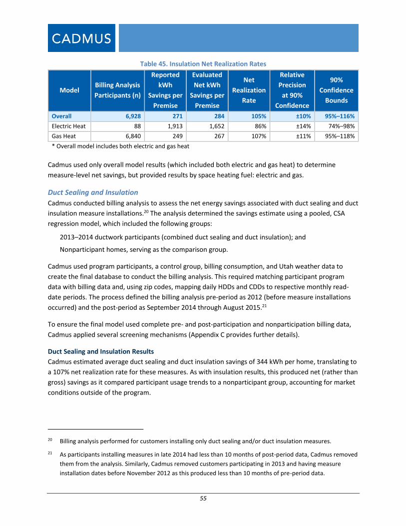
55
Table 45. Insulation Net Realization Rates
Model Billing Analysis
Participants (n)
Reported
kWh
Savings per
Premise
Evaluated
Net kWh
Savings per
Premise
Net
Realization
Rate
Relative
Precision
at 90%
Confidence
90%
Confidence
Bounds
Overall 6,928 271 284 105% ±10% 95%–116%
Electric Heat 88 1,913 1,652 86% ±14% 74%–98%
Gas Heat 6,840 249 267 107% ±11% 95%–118%
* Overall model includes both electric and gas heat
Cadmus used only overall model results (which included both electric and gas heat) to determine
measure-level net savings, but provided results by space heating fuel: electric and gas.
Duct Sealing and Insulation
Cadmus conducted billing analysis to assess the net energy savings associated with duct sealing and duct
insulation measure installations.20 The analysis determined the savings estimate using a pooled, CSA
regression model, which included the following groups:
2013–2014 ductwork participants (combined duct sealing and duct insulation); and
Nonparticipant homes, serving as the comparison group.
Cadmus used program participants, a control group, billing consumption, and Utah weather data to
create the final database to conduct the billing analysis. This required matching participant program
data with billing data and, using zip codes, mapping daily HDDs and CDDs to respective monthly read-
date periods. The process defined the billing analysis pre-period as 2012 (before measure installations
occurred) and the post-period as September 2014 through August 2015.21
To ensure the final model used complete pre- and post-participation and nonparticipation billing data,
Cadmus applied several screening mechanisms (Appendix C provides further details).
Duct Sealing and Insulation Results
Cadmus estimated average duct sealing and duct insulation savings of 344 kWh per home, translating to
a 107% net realization rate for these measures. As with insulation results, this produced net (rather than
gross) savings as it compared participant usage trends to a nonparticipant group, accounting for market
conditions outside of the program.
20 Billing analysis performed for customers installing only duct sealing and/or duct insulation measures.
21 As participants installing measures in late 2014 had less than 10 months of post-period data, Cadmus removed
them from the analysis. Similarly, Cadmus removed customers participating in 2013 and having measure
installation dates before November 2012 as this produced less than 10 months of pre-period data.

56
With average participant pre-usage of 10,925 kWh, savings represented a 3% reduction in total energy
usage from duct sealing and duct insulation measures installed. Table 46 presents the overall savings
estimate for duct sealing and duct insulation.
Table 46. Ductwork Net Realization Rates
Model
Billing
Analysis
Participant (n)
Reported
kWh Savings
per Premise
Evaluated Net
kWh Savings
per Premise
Net
Realization
Rate
Relative
Precision
at 90%
Confidence
90%
Confidence
Bounds
Overall 753 323 344 107% ±23% 82%–131%
Electric Heat 7 2,472 1,683 68% ±44% 38%–98%
Gas Heat 746 303 331 110% ±24% 84%–135%
* Overall model includes both electric and gas heat
Cadmus only used overall model results (electric and gas heat combined) to determine measure-level
net savings, but provided results by space heating fuel: electric and non-electric. Overall, electrically
heated homes achieved duct sealing and duct insulation savings of 1,683 kWh per home.
Central Air Conditioners and Evaporative Coolers
Cadmus conducted billing analyses to assess gross energy savings associated with high-efficiency air
conditioners and evaporative coolers. The analysis required construction of three regression models
(Appendix C provides further details on the regression model):
1. A central air conditioner and sizing and installation measures (SEER 15+) model22
2. An evaporative cooling model
3. A model of SEER 13 nonparticipant units (to serve as a baseline)23
Cadmus used program participants, billing consumption, Utah weather, and square footage data to
create the final database for conducting the billing analysis, the results of which provided gross
realization rates for central air conditioners and evaporative cooler equipment types across both years.
This billing analysis resulted in gross savings (as opposed to the net savings that the billing analysis for
ductwork and insulations estimated) due of the nature of the comparisons group used. The central air
conditioner and evaporative cooler comparison group did not reflect the average market conditions as
22 This model contained sizing + TXV (thermal expansion valve) and proper installation central air-conditioning
measures. It calculated a realization rate applying to all of these measures.
23 This assessment adopted a central assumption: participants would have installed a base-efficiency (13 SEER)
unit had they not participated in the program. Given this, Cadmus used a control group composed of 2005
Cool Cash Program participants known to have received a 13 SEER air-conditioning unit—without sizing + TXV
or proper installation incentives—as their primary cooling system. SEER 13 air-conditioning equipment
represents the federal minimum efficiency level for residential central air conditioners manufactured after
January 2006.
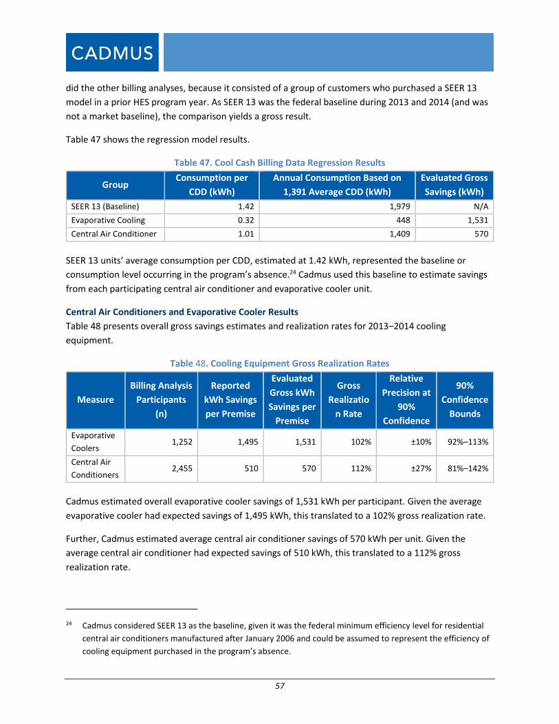
57
did the other billing analyses, because it consisted of a group of customers who purchased a SEER 13
model in a prior HES program year. As SEER 13 was the federal baseline during 2013 and 2014 (and was
not a market baseline), the comparison yields a gross result.
Table 47 shows the regression model results.
Table 47. Cool Cash Billing Data Regression Results
Group Consumption per
CDD (kWh)
Annual Consumption Based on
1,391 Average CDD (kWh)
Evaluated Gross
Savings (kWh)
SEER 13 (Baseline) 1.42 1,979 N/A
Evaporative Cooling 0.32 448 1,531
Central Air Conditioner 1.01 1,409 570
SEER 13 units’ average consumption per CDD, estimated at 1.42 kWh, represented the baseline or
consumption level occurring in the program’s absence.24 Cadmus used this baseline to estimate savings
from each participating central air conditioner and evaporative cooler unit.
Central Air Conditioners and Evaporative Cooler Results
Table 48 presents overall gross savings estimates and realization rates for 2013–2014 cooling
equipment.
Table 48. Cooling Equipment Gross Realization Rates
Measure
Billing Analysis
Participants
(n)
Reported
kWh Savings
per Premise
Evaluated
Gross kWh
Savings per
Premise
Gross
Realizatio
n Rate
Relative
Precision at
90%
Confidence
90%
Confidence
Bounds
Evaporative
Coolers 1,252 1,495 1,531 102% ±10% 92%–113%
Central Air
Conditioners 2,455 510 570 112% ±27% 81%–142%
Cadmus estimated overall evaporative cooler savings of 1,531 kWh per participant. Given the average
evaporative cooler had expected savings of 1,495 kWh, this translated to a 102% gross realization rate.
Further, Cadmus estimated average central air conditioner savings of 570 kWh per unit. Given the
average central air conditioner had expected savings of 510 kWh, this translated to a 112% gross
realization rate.
24 Cadmus considered SEER 13 as the baseline, given it was the federal minimum efficiency level for residential
central air conditioners manufactured after January 2006 and could be assumed to represent the efficiency of
cooling equipment purchased in the program’s absence.
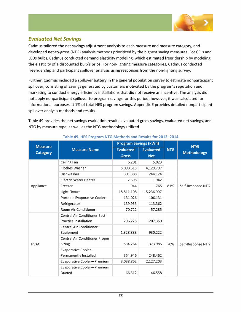
58
Evaluated Net Savings Cadmus tailored the net savings adjustment analysis to each measure and measure category, and
developed net-to-gross (NTG) analysis methods prioritized by the highest saving measures. For CFLs and
LEDs bulbs, Cadmus conducted demand elasticity modeling, which estimated freeridership by modeling
the elasticity of a discounted bulb’s price. For non-lighting measure categories, Cadmus conducted
freeridership and participant spillover analysis using responses from the non-lighting survey.
Further, Cadmus included a spillover battery in the general population survey to estimate nonparticipant
spillover, consisting of savings generated by customers motivated by the program’s reputation and
marketing to conduct energy efficiency installations that did not receive an incentive. The analysis did
not apply nonparticipant spillover to program savings for this period, however, it was calculated for
informational purposes at 1% of total HES program savings. Appendix E provides detailed nonparticipant
spillover analysis methods and results.
Table 49 provides the net savings evaluation results: evaluated gross savings, evaluated net savings, and
NTG by measure type, as well as the NTG methodology utilized.
Table 49. HES Program NTG Methods and Results for 2013–2014
Measure
Category Measure Name
Program Savings (kWh)
NTG NTG
Methodology Evaluated
Gross
Evaluated
Net
Appliance
Ceiling Fan 6,201 5,023
81% Self-Response NTG
Clothes Washer 5,098,515 4,129,797
Dishwasher 301,388 244,124
Electric Water Heater 2,398 1,942
Freezer 944 765
Light Fixture 18,811,108 15,236,997
Portable Evaporative Cooler 131,026 106,131
Refrigerator 139,953 113,362
Room Air Conditioner 70,722 57,285
HVAC
Central Air Conditioner Best
Practice Installation 296,228 207,359
70% Self-Response NTG
Central Air Conditioner
Equipment 1,328,888 930,222
Central Air Conditioner Proper
Sizing 534,264 373,985
Evaporative Cooler—
Permanently Installed 354,946 248,462
Evaporative Cooler—Premium 3,038,862 2,127,203
Evaporative Cooler—Premium
Ducted 66,512 46,558
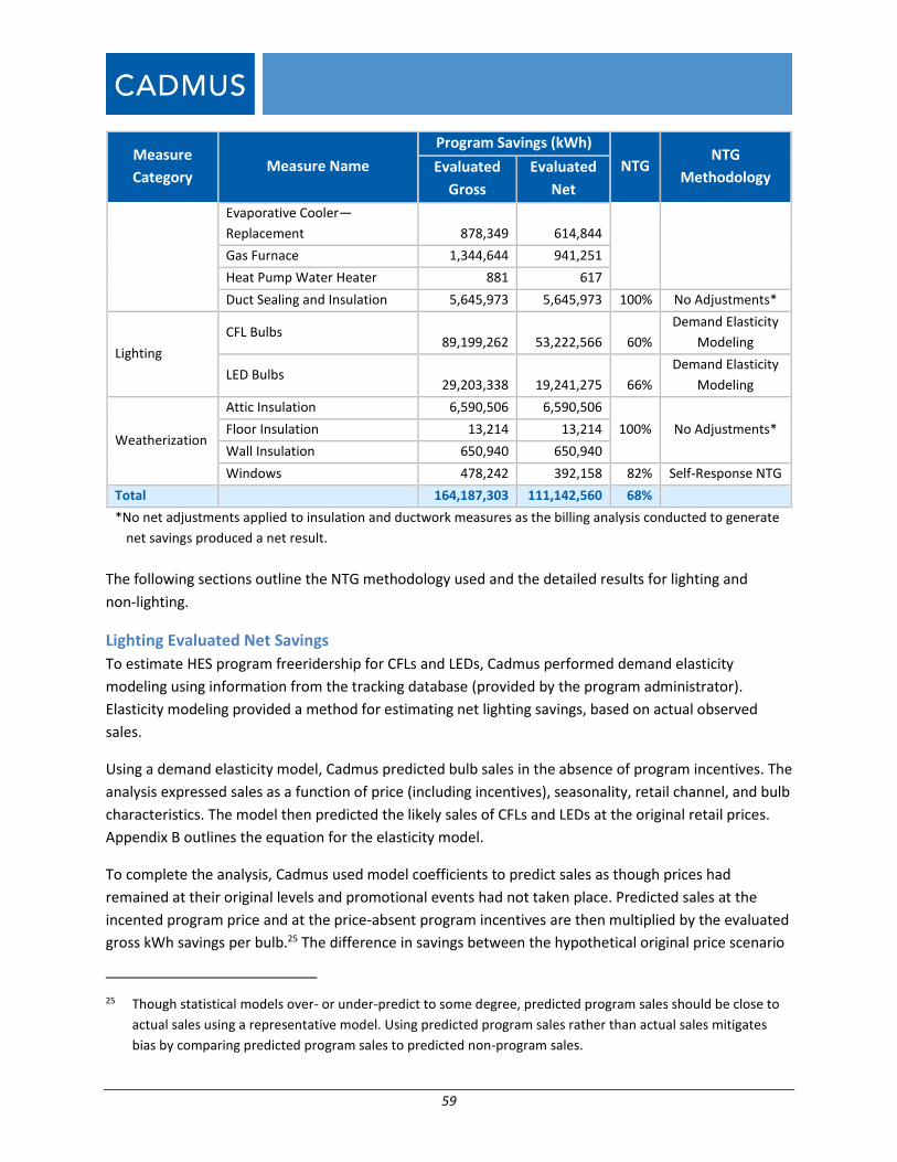
59
Measure
Category Measure Name
Program Savings (kWh)
NTG NTG
Methodology Evaluated
Gross
Evaluated
Net
Evaporative Cooler—
Replacement 878,349 614,844
Gas Furnace 1,344,644 941,251
Heat Pump Water Heater 881 617
Duct Sealing and Insulation 5,645,973 5,645,973 100% No Adjustments*
Lighting
CFL Bulbs 89,199,262 53,222,566 60%
Demand Elasticity
Modeling
LED Bulbs 29,203,338 19,241,275 66%
Demand Elasticity
Modeling
Weatherization
Attic Insulation 6,590,506 6,590,506
100% No Adjustments* Floor Insulation 13,214 13,214
Wall Insulation 650,940 650,940
Windows 478,242 392,158 82% Self-Response NTG
Total 164,187,303 111,142,560 68%
*No net adjustments applied to insulation and ductwork measures as the billing analysis conducted to generate
net savings produced a net result.
The following sections outline the NTG methodology used and the detailed results for lighting and
non-lighting.
Lighting Evaluated Net Savings
To estimate HES program freeridership for CFLs and LEDs, Cadmus performed demand elasticity
modeling using information from the tracking database (provided by the program administrator).
Elasticity modeling provided a method for estimating net lighting savings, based on actual observed
sales.
Using a demand elasticity model, Cadmus predicted bulb sales in the absence of program incentives. The
analysis expressed sales as a function of price (including incentives), seasonality, retail channel, and bulb
characteristics. The model then predicted the likely sales of CFLs and LEDs at the original retail prices.
Appendix B outlines the equation for the elasticity model.
To complete the analysis, Cadmus used model coefficients to predict sales as though prices had
remained at their original levels and promotional events had not taken place. Predicted sales at the
incented program price and at the price-absent program incentives are then multiplied by the evaluated
gross kWh savings per bulb.25 The difference in savings between the hypothetical original price scenario
25 Though statistical models over- or under-predict to some degree, predicted program sales should be close to
actual sales using a representative model. Using predicted program sales rather than actual sales mitigates
bias by comparing predicted program sales to predicted non-program sales.
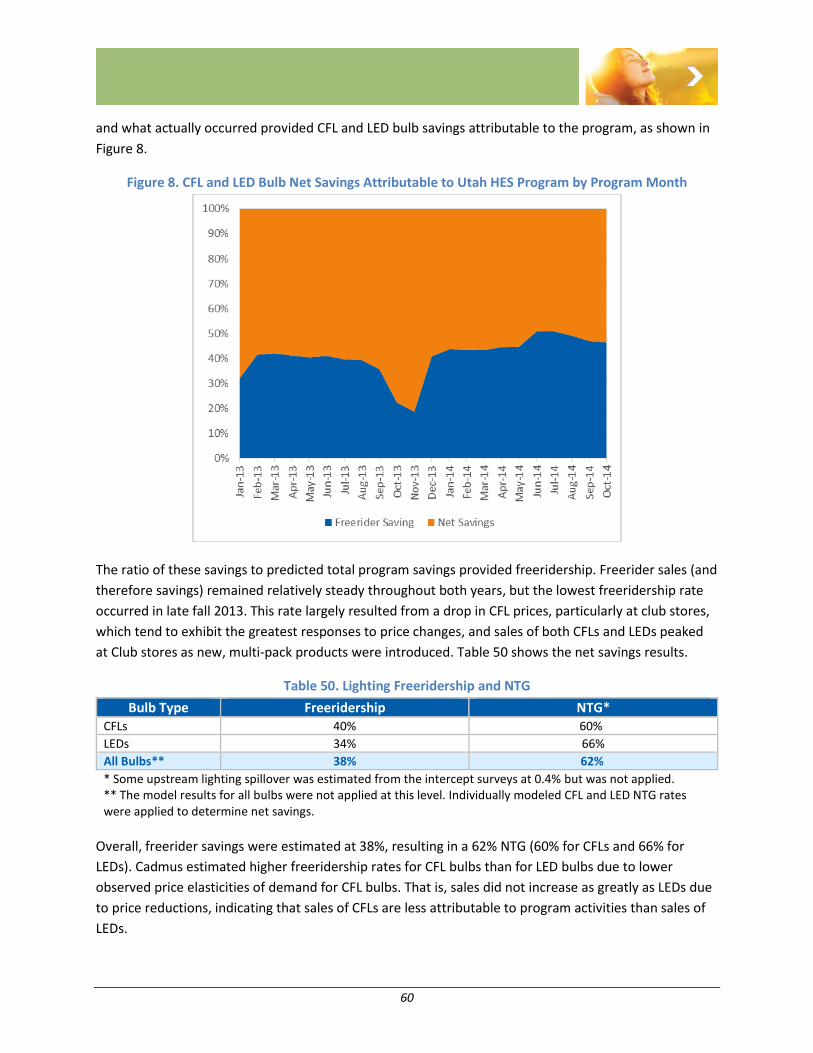
60
and what actually occurred provided CFL and LED bulb savings attributable to the program, as shown in
Figure 8.
Figure 8. CFL and LED Bulb Net Savings Attributable to Utah HES Program by Program Month
The ratio of these savings to predicted total program savings provided freeridership. Freerider sales (and
therefore savings) remained relatively steady throughout both years, but the lowest freeridership rate
occurred in late fall 2013. This rate largely resulted from a drop in CFL prices, particularly at club stores,
which tend to exhibit the greatest responses to price changes, and sales of both CFLs and LEDs peaked
at Club stores as new, multi-pack products were introduced. Table 50 shows the net savings results.
Table 50. Lighting Freeridership and NTG
Bulb Type Freeridership NTG* CFLs 40% 60%
LEDs 34% 66%
All Bulbs** 38% 62%
* Some upstream lighting spillover was estimated from the intercept surveys at 0.4% but was not applied. ** The model results for all bulbs were not applied at this level. Individually modeled CFL and LED NTG rates were applied to determine net savings.
Overall, freerider savings were estimated at 38%, resulting in a 62% NTG (60% for CFLs and 66% for
LEDs). Cadmus estimated higher freeridership rates for CFL bulbs than for LED bulbs due to lower
observed price elasticities of demand for CFL bulbs. That is, sales did not increase as greatly as LEDs due
to price reductions, indicating that sales of CFLs are less attributable to program activities than sales of
LEDs.
61
As shown in Table 51, Cadmus also estimated freeridership by distribution channel. Upon predicting
monthly savings for each individual bulb model, as described above, Cadmus aggregated the results by
retail channel and bulb type. Taking the difference between predicted savings with the program and in
the program’s absence provides freeridership estimates by retail channels and bulb types.
Table 51. Per-Bulb Price and Freeridership by Retail Channel and Bulb Type
Retail Channel Bulb Type Average Original
Price Per Bulb
Average Final
Price Per Bulb Markdown % Freeridership
Non-Club Store CFL $ 2.56 $ 1.25 51% 56%
LED $ 15.37 $10.61 31% 77%
Club Store CFL $ 1.96 $ 0.67 66% 34%
LED $ 9.74 $ 4.99 49% 30%
Freeridership was lower at club stores than at non-club stores, both for LEDs and CFLs. This likely
resulted from a number of factors:
The price elasticities at club stores are greater than those at non-club stores, particularly for LEDs,
which were more than twice the non-club store elasticities26. This suggests club store shoppers tend
to be more sensitive to price changes, the same proportional markdown (i.e., the incentive as a
share of the original price) led to a greater increase in sales at club stores compared to non-club
stores.
As shown in Table 51, incentive levels were higher at club stores than at non-club stores for both
CFLs and LEDs. This contributed to average per-bulb prices at club stores roughly one-half of per-
bulb prices at non-club stores.
Club stores offer a different product mix compared to non-club stores, with club stores often only
stocking a few options for the most commonly purchased products and not dedicating much shelf
space to products with more limited uses.
Big-box, non-club retailers, accounting for the majority of non-club store sales, tend to stock a wide
assortment of products, some with limited, specialty applications. Demand for these products tends
to be the least elastic, lowering average elasticities within a retail channel.
Appendix B provides a detailed report on the price response modeling methodology and results.
Freeridership Comparisons
Table 52 compares CFL freeridership estimates from several recent evaluations using the elasticity
model approach. The table also shows the average, sales-weighted original retail price of program bulbs
and the markdown as a percent of the original price, which is a significant driver of freeridership
estimates.
26 LED elasticities for general purpose bulbs were 1.706 at club stores compared to 0.743 at non-club stores. Full model details and detailed elasticity estimates are included in Appendix B.
62
The freeridership estimates for Rocky Mountain Power are within the range of those observed in other
programs, however, they have increased since the 2011-2012 modeling effort. Part of the increase may
be the maturation of the efficient lighting market. As CFLs become a more familiar and accepted
technology, demand may become less elastic – that is, for those consumers who are willing to substitute
CFLs for less efficient bulbs, their willingness to buy CFLs may have become less dependent on
promotional activities over time. Some of this effect may be due to utility-sponsored programs, such as
the Rocky Mountain Power program, as well factors such as improved lighting quality and customers
realizing energy savings from switching to CFLs. And for those that are less inclined to substitute CFLs,
their decision may remain the same regardless of price changes.
Saturation of CFLs could be another factor. Customers that responded to price drops in 2011 or 2012
and stocked up on CFLs may buy fewer bulbs in subsequent years if they still have previously purchased
bulbs in storage.
Another potential factor could be the lack of merchandising data. Without data to explicitly control for
sales lift due to merchandising in either evaluation, there is an unobserved variable influencing sales.
Because the model is trying to explain variation in sales over time, the price elasticity estimates may
absorb some of the impact of product merchandising to the degree that merchandising and price
changes co-vary. That is to say, if prices decrease are observed and sales increase at the same time, but
there are also promotions occurring at the same time but are unobserved, the model will attribute the
change in sales to the price change because that is the variable that is observed.
Table 52. Comparisons of CFL Freeridership and Incentive Levels
Utility Bulb
Type
Average
Original Price
per bulb
Average
Markdown
per bulb
Markdown
% Freeridership
Rocky Mountain Power Utah
2011-2012 Standard $2.18 $1.37 63% 17%
Mid-Atlantic Utility 1 Standard $1.97 $1.41 72% 27%
Mid-Atlantic Utility 3 Standard $2.10 $1.59 76% 27%
New England Standard $2.11 $1.00 47% 32%
Mid-Atlantic Utility 2 Standard $2.14 $1.43 67% 35%
Mid-Atlantic Utility 4 Standard $2.22 $1.46 66% 35%
Rocky Mountain Power
Utah 2013-2014 Standard $2.21 $1.30 58% 40%
Midwest Utility Standard $1.82 $1.13 62% 43%
Southeast Standard $2.15 $1.09 51% 48%
63
Table 53 shows LED freeridership estimates for four other recent evaluations. Additional details for
markdown levels and prices are not provided because the retail and product mix varies considerably
between evaluations, which is a major factor in the per-bulb prices. The Rocky Mountain Power Utah
program is in the lower range of observed freeridership estimates.
Table 53. Comparison of LED Freeridership
Utility Freeridership
Wisconsin (2015) 29%
Midwest (2014) 30%
Rocky Mountain Power Utah (2013-2014) 34%
South (2015) 48%
Mid-Atlantic (2014-2015) 48%
Upstream Lighting Spillover
Upstream participant lighting spillover was estimated from the intercept surveys at 0.4% (the Intercept
Survey Spillover section outlines the methodology). That is, for every 1,000 kWh of evaluated gross
savings, an additional 4 kWh of unreported savings may have occurred as a result of the program’s
operation. This value, however, was not applied due to the nature of sampling which was prioritized by
the leakage study. The majority of stores that Cadmus visited were on the edges and outside of Rocky
Mountain Power’s service territory, and therefore the results did not represent the full picture of
spillover occurring from the upstream lighting incentives, and likely provided a low estimate. Also,
spillover proves particularly difficult to measure for upstream programs. As customers often remain
unaware of their participation in the program, they generally cannot identify its influence on other
purchasing decisions.
Non-Lighting Evaluated Net Savings
Cadmus relied on the non-lighting participant survey to determine non-lighting NTG for appliance,
HVAC, and weatherization measure categories for 2013 and 2014 participants.
Freeridership and participant spillover constitute the NTG. Cadmus used the following formula to
determine the final NTG ratio for each non-lighting program measure:
Net-to-gross ratio = (1 – Freeridership) + Spillover
Methodology
Cadmus determined the freeridership amount based on a previously developed approach for Rocky
Mountain Power, which ascertained freeridership using patterns of responses to a series of survey
questions. These questions—answered as “yes,” “no,” or “don’t know”—asked whether participants
would have installed the same equipment in the program’s absence, at the same time, amount, and
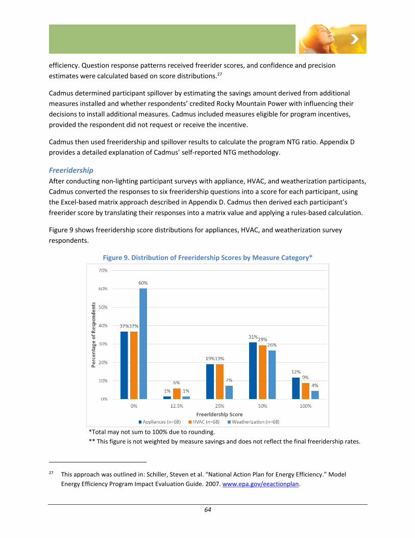
64
efficiency. Question response patterns received freerider scores, and confidence and precision
estimates were calculated based on score distributions.27
Cadmus determined participant spillover by estimating the savings amount derived from additional
measures installed and whether respondents’ credited Rocky Mountain Power with influencing their
decisions to install additional measures. Cadmus included measures eligible for program incentives,
provided the respondent did not request or receive the incentive.
Cadmus then used freeridership and spillover results to calculate the program NTG ratio. Appendix D
provides a detailed explanation of Cadmus’ self-reported NTG methodology.
Freeridership
After conducting non-lighting participant surveys with appliance, HVAC, and weatherization participants,
Cadmus converted the responses to six freeridership questions into a score for each participant, using
the Excel-based matrix approach described in Appendix D. Cadmus then derived each participant’s
freerider score by translating their responses into a matrix value and applying a rules-based calculation.
Figure 9 shows freeridership score distributions for appliances, HVAC, and weatherization survey
respondents.
Figure 9. Distribution of Freeridership Scores by Measure Category*
*Total may not sum to 100% due to rounding.
** This figure is not weighted by measure savings and does not reflect the final freeridership rates.
27 This approach was outlined in: Schiller, Steven et al. “National Action Plan for Energy Efficiency.” Model
Energy Efficiency Program Impact Evaluation Guide. 2007. www.epa.gov/eeactionplan.
65
Approximately 37% of appliance and HVAC measure respondents and 60% of weatherization
respondents indicated no freeridership. That is, they would not have purchased the efficient measure in
the absence of Rocky Mountain Power’s program. More appliance respondents indicated high
freeridership (scores of 50-100%) than the other measure categories.
Spillover
This section presents the results from additional, energy-efficient measures customers installed after
participating in the HES program. While many participants installed such measures after receiving
incentives from Rocky Mountain Power, Cadmus only attributed program spillover to additional
purchases significantly influenced by HES program participation and not claimed through the program.
Only one respondent—an HVAC participant—fell into this category.
Cadmus used evaluated savings values from the deemed savings analysis to estimate spillover measure
savings. This involved estimating the spillover percentage for the HVAC measure category by dividing the
sum of the additional spillover savings by the total incentivized gross savings achieved by all 68 HVAC
respondents. Table 54 shows the results.
Table 54. Non-Lighting Spillover Responses
Measure
Category
Spillover Measure
Installed Quantity
Electric Savings
(kWh)
Surveyed Measure
Category Savings
Spillover
Ratio
HVAC Furnace 1 477 35,915 1%
Non-Lighting NTG Findings
Cadmus conducted 68 surveys with participants in each measure category (appliance, HVAC and
weatherization) to generate NTG ratios ranging from 70% for HVAC measures to 82% for weatherization.
Table 55 summarizes these findings.
Table 55. Non-Lighting NTG Ratio by Measure Category
Program
Category Responses (n)
Freeridership
Ratio
Spillover
Ratio NTG
Absolute Precision
at 90% Confidence
Appliances 68 19% 0% 81% ±6%
HVAC 68 31% 1% 70% ±9%
Weatherization 68 18% 0% 82% ±6%
*Weighted by evaluated program savings.
The NTG column indicates the percentage of gross savings attributable to the program. For example,
participants purchasing an appliance measure received an 81% NTG, indicating that 81% of gross savings
for appliance measures could be attributed to the HES program.
Table 56 shows freeridership, spillover, and NTG estimates for appliance and HVAC rebate programs
reported for prior Rocky Mountain Power program years as well as for other utilities with similar
programs and measure offerings.

66
Table 56. Non-Lighting NTG Comparisons*
Utility/Region Reported
Year
Responses
(n) FR** %
Spillover
% NTG
Appliances
Rocky Mountain Power Utah 2013–2014
HES Evaluation: Appliances 2016 68 19% 0% 81%
Rocky Mountain Power Utah 2011–2012
HES Evaluation: Appliances 2013 247 42% 8% 66%
Northeast Utility—Appliances 2015 65 65% 3% 38%
Northwest Utility—Appliances 2014 73 79% 2% 23 %
HVAC
Rocky Mountain Power Utah 2011–2012
HES Evaluation: HVAC 2013 64 11% 0% 89%
Rocky Mountain Power Utah 2013–2014
HES Evaluation: HVAC 2016 68 31% 1% 70%
Midwest Utility—HVAC 2015 73 51% 1% 50%
Northwest Utility—HVAC 2014 48 72% 1% 29%
Weatherization
Rocky Mountain Power Utah 2013–2014
HES Evaluation: Weatherization 2016 68 18% 0% 82%
Midwest Utility—Weatherization 2015 208 30% 2% 72%
Midwest Utility—Weatherization 2015 79 36% 2% 66%
*NTG values derive from self-response surveys, though differences in analysis and scoring methodologies may vary
across evaluations.
**Freeridership.
For the appliance measure category, fewer respondents in 2013–2014 reported already purchasing
measures before learning of the program—the largest driver of the NTG increase compared with the
2011–2012 evaluation. Fewer appliance measure category respondents in 2013-2014 reported that they
would have purchased a measure at the same efficiency level within one year without the HES program
incentive compared to 2011-2012 respondents. These shifts in freeridership response patterns are key
contributing factors to HES appliance freeridership rates decreasing since the prior evaluation.
Another contributing factor to the drop in appliance measure category freeridership since the 2011-
2012 evaluation is that lighting fixture respondents represented 47% of total appliance measure
category responses in the 2013–2014 analysis and lighting fixture respondents indicated an average 7%
freeridership rate. In the 2011–2012 appliance measure category’s freeridership analysis sample,
lighting fixture respondents represented 28% of the appliance category analysis sample, with an
average, estimated freeridership rate of 27%. All other appliance measure level freeridership estimates
in the 2011–2012 and 2013–2014 evaluations were over 38%.
67
The 2013–2014 HVAC measure category exhibited a NTG estimate of 70%, which is higher than other
utilities’ comparable HVAC programs, but lower than the 89% estimate for 2011–2012 HVAC NTG.
Comparing HVAC NTG ratios across evaluation years for HES proved challenging due to different
measure categories in the participant sample. The 2011–2012 evaluation mostly included duct sealing
and duct insulation respondents, while the 2013–2014 respondents received HES rebates for central air
conditioners, evaporative coolers, furnaces, and room air conditioners measures. Compared to the
2011–2012 HVAC NTG estimate, the 2013–2014 HVAC NTG came closer to NTG estimates from other
recent utility evaluations with similar HVAC program measure offerings.
In 2013–2014, the weatherization measure category’s 82% NTG estimate was higher than for other
utilities’ comparable weatherization programs. The 2011–2012 Utah HES Evaluation did not include a
weatherization NTG estimate.
Lighting Leakage Study Cadmus conducted intercept surveys at stores in Utah, Idaho, and Washington which were designed to
determine how many light bulbs purchased within PacifiCorp’s territory had been installed outside of
PacifiCorp’s territory—generally referred to as leakage.28 Cadmus also conducted intercept surveys at
stores outside of PacifiCorp’s territory to determine the percentage of those light bulbs installed within
PacifiCorp’s territory. Given the low number of surveys completed in Washington and Idaho, and that
the RSAT algorithm is the same across states, Cadmus combined the results for all states to show key
findings along with Utah-specific results.
The leakage study sought to test scores from PacifiCorp’s RSAT, developed to determine the best stores
for cost-effectively offering discounted energy-efficient light bulbs. The Retailer Allocation Review in
Appendix F describes the RSAT; this section also discusses the leakage study’s methodology and results.
Overall, Cadmus found that the RSAT is performing well. While there is some variation in the results by
store, particularly when the number of intercept surveys we were able to conduct in a store were low,
the RSAT scores were within our estimate range of leakage scores calculated from the intercept survey
responses. Cadmus found that lighting leakage rates were an average of roughly 5.1 percentage points
higher than predicted by the RSAT, with a confidence level of 90% and precision of ± 5.3%.
Methodology
Cadmus targeted 20 Utah stores for intercept surveys—15 stores in Rocky Mountain Power’s service
territory and five stores outside its territory. Of the 15 stores in the service territory, Cadmus established
targets of eight stores with RSAT scores greater than or equal to 96% and seven stores with RSAT scores
less than 96%, which included 34 nonparticipating stores.
28 This study did not review internet lighting purchases, only those made at a brick and mortar stores.
68
The program administrator provided Cadmus with store rosters for each state. These included retailer
addresses, phone numbers, and RSAT scores, and indicated each store’s location within the service
territory. For stores outside of the territory, Cadmus created a roster for each state, using Pacific
Power’s and Rocky Mountain Power’s service area maps29 to select cities/territories near the service
territory. Cadmus then used Google Maps to identify all relevant retailers in the specified areas,
supplemented by phone calls to the stores to verify they were outside of Rocky Mountain Power’s
territory.
To set up store visits, a Cadmus representative called a targeted store and asked for a manager or
another employee in charge of daily operations. Representatives then used a script as a guide in
explaining the study’s purpose and Cadmus’ intention in conducting intercept surveys at their stores. By
calling ahead, Cadmus sought to ensure store visits by Cadmus field technicians would not only be
authorized but welcome. From late October to early December (depending on contact availability),
Cadmus attempted to contact each store’s manager or owner until it was able to confirm whether the
store manager would or would not participate (consequently, the study contacted many stores more
than once). For each store authorizing the intercept surveys, Cadmus used phone contacts to schedule
two-day visits, and, field technicians followed up with each store in advance of the visit to remind them
of the appointments.
Cadmus achieved more success in scheduling visits with independent retailers or independently owned
franchises than with big-box home and hardware stores. Managers of large retail chains (e.g., Home
Depot, Lowe’s, Bed Bath & Beyond, Walmart, Target, Albertson’s, Dollar Tree) frequently redirected
Cadmus to their corporate offices, which most commonly resulted in rejections or nonresponses to the
contact attempts. This is explored further in the section: Leakage Survey Results by Store Size.
This difficulty gaining cooperation of big-box stores limited the number of surveys Cadmus could
complete, given the extensive foot traffic large retailers draw. Further, Cadmus observed that stores’
agreed participation rates—about one in eight stores contacted—would likely prevent achievement of
the original targets.
29 https://www.rockymountainpower.net/content/dam/pacificorp/doc/About_Us/Company_Overview/PC-10k-
ServiceAreaMap-2015-v2.pdf
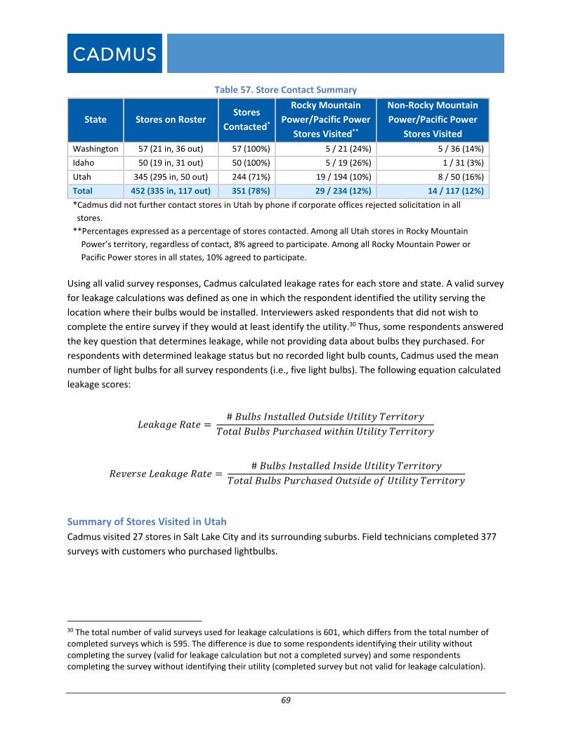
69
Table 57. Store Contact Summary
State Stores on Roster Stores
Contacted*
Rocky Mountain
Power/Pacific Power
Stores Visited**
Non-Rocky Mountain
Power/Pacific Power
Stores Visited
Washington 57 (21 in, 36 out) 57 (100%) 5 / 21 (24%) 5 / 36 (14%)
Idaho 50 (19 in, 31 out) 50 (100%) 5 / 19 (26%) 1 / 31 (3%)
Utah 345 (295 in, 50 out) 244 (71%) 19 / 194 (10%) 8 / 50 (16%)
Total 452 (335 in, 117 out) 351 (78%) 29 / 234 (12%) 14 / 117 (12%)
*Cadmus did not further contact stores in Utah by phone if corporate offices rejected solicitation in all
stores.
**Percentages expressed as a percentage of stores contacted. Among all Utah stores in Rocky Mountain
Power’s territory, regardless of contact, 8% agreed to participate. Among all Rocky Mountain Power or
Pacific Power stores in all states, 10% agreed to participate.
Using all valid survey responses, Cadmus calculated leakage rates for each store and state. A valid survey
for leakage calculations was defined as one in which the respondent identified the utility serving the
location where their bulbs would be installed. Interviewers asked respondents that did not wish to
complete the entire survey if they would at least identify the utility.30 Thus, some respondents answered
the key question that determines leakage, while not providing data about bulbs they purchased. For
respondents with determined leakage status but no recorded light bulb counts, Cadmus used the mean
number of light bulbs for all survey respondents (i.e., five light bulbs). The following equation calculated
leakage scores:
𝐿𝑒𝑎𝑘𝑎𝑔𝑒 𝑅𝑎𝑡𝑒 = # 𝐵𝑢𝑙𝑏𝑠 𝐼𝑛𝑠𝑡𝑎𝑙𝑙𝑒𝑑 𝑂𝑢𝑡𝑠𝑖𝑑𝑒 𝑈𝑡𝑖𝑙𝑖𝑡𝑦 𝑇𝑒𝑟𝑟𝑖𝑡𝑜𝑟𝑦
𝑇𝑜𝑡𝑎𝑙 𝐵𝑢𝑙𝑏𝑠 𝑃𝑢𝑟𝑐ℎ𝑎𝑠𝑒𝑑 𝑤𝑖𝑡ℎ𝑖𝑛 𝑈𝑡𝑖𝑙𝑖𝑡𝑦 𝑇𝑒𝑟𝑟𝑖𝑡𝑜𝑟𝑦
𝑅𝑒𝑣𝑒𝑟𝑠𝑒 𝐿𝑒𝑎𝑘𝑎𝑔𝑒 𝑅𝑎𝑡𝑒 = # 𝐵𝑢𝑙𝑏𝑠 𝐼𝑛𝑠𝑡𝑎𝑙𝑙𝑒𝑑 𝐼𝑛𝑠𝑖𝑑𝑒 𝑈𝑡𝑖𝑙𝑖𝑡𝑦 𝑇𝑒𝑟𝑟𝑖𝑡𝑜𝑟𝑦
𝑇𝑜𝑡𝑎𝑙 𝐵𝑢𝑙𝑏𝑠 𝑃𝑢𝑟𝑐ℎ𝑎𝑠𝑒𝑑 𝑂𝑢𝑡𝑠𝑖𝑑𝑒 𝑜𝑓 𝑈𝑡𝑖𝑙𝑖𝑡𝑦 𝑇𝑒𝑟𝑟𝑖𝑡𝑜𝑟𝑦
Summary of Stores Visited in Utah
Cadmus visited 27 stores in Salt Lake City and its surrounding suburbs. Field technicians completed 377
surveys with customers who purchased lightbulbs.
30 The total number of valid surveys used for leakage calculations is 601, which differs from the total number of completed surveys which is 595. The difference is due to some respondents identifying their utility without completing the survey (valid for leakage calculation but not a completed survey) and some respondents completing the survey without identifying their utility (completed survey but not valid for leakage calculation).
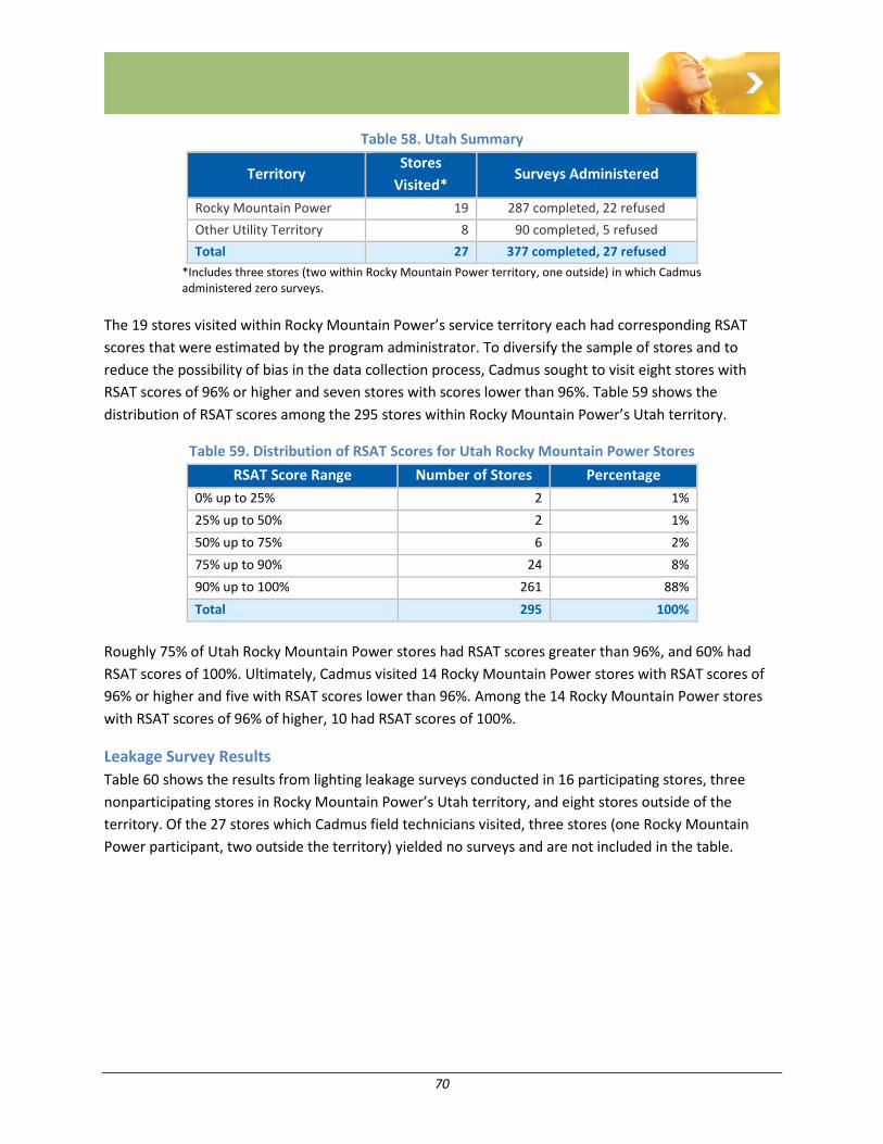
70
Table 58. Utah Summary
Territory Stores
Visited* Surveys Administered
Rocky Mountain Power 19 287 completed, 22 refused
Other Utility Territory 8 90 completed, 5 refused
Total 27 377 completed, 27 refused
*Includes three stores (two within Rocky Mountain Power territory, one outside) in which Cadmus administered zero surveys.
The 19 stores visited within Rocky Mountain Power’s service territory each had corresponding RSAT
scores that were estimated by the program administrator. To diversify the sample of stores and to
reduce the possibility of bias in the data collection process, Cadmus sought to visit eight stores with
RSAT scores of 96% or higher and seven stores with scores lower than 96%. Table 59 shows the
distribution of RSAT scores among the 295 stores within Rocky Mountain Power’s Utah territory.
Table 59. Distribution of RSAT Scores for Utah Rocky Mountain Power Stores
RSAT Score Range Number of Stores Percentage
0% up to 25% 2 1%
25% up to 50% 2 1%
50% up to 75% 6 2%
75% up to 90% 24 8%
90% up to 100% 261 88%
Total 295 100%
Roughly 75% of Utah Rocky Mountain Power stores had RSAT scores greater than 96%, and 60% had
RSAT scores of 100%. Ultimately, Cadmus visited 14 Rocky Mountain Power stores with RSAT scores of
96% or higher and five with RSAT scores lower than 96%. Among the 14 Rocky Mountain Power stores
with RSAT scores of 96% of higher, 10 had RSAT scores of 100%.
Leakage Survey Results
Table 60 shows the results from lighting leakage surveys conducted in 16 participating stores, three
nonparticipating stores in Rocky Mountain Power’s Utah territory, and eight stores outside of the
territory. Of the 27 stores which Cadmus field technicians visited, three stores (one Rocky Mountain
Power participant, two outside the territory) yielded no surveys and are not included in the table.
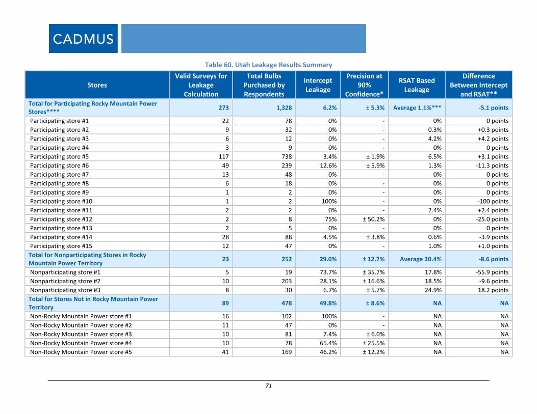
71
Table 60. Utah Leakage Results Summary
Stores Valid Surveys for
Leakage Calculation
Total Bulbs Purchased by Respondents
Intercept Leakage
Precision at 90%
Confidence*
RSAT Based Leakage
Difference Between Intercept
and RSAT** Total for Participating Rocky Mountain Power Stores****
273 1,328 6.2% ± 5.3% Average 1.1%*** -5.1 points
Participating store #1 22 78 0% - 0% 0 points
Participating store #2 9 32 0% - 0.3% +0.3 points
Participating store #3 6 12 0% - 4.2% +4.2 points
Participating store #4 3 9 0% - 0% 0 points
Participating store #5 117 738 3.4% ± 1.9% 6.5% +3.1 points
Participating store #6 49 239 12.6% ± 5.9% 1.3% -11.3 points
Participating store #7 13 48 0% - 0% 0 points
Participating store #8 6 18 0% - 0% 0 points
Participating store #9 1 2 0% - 0% 0 points
Participating store #10 1 2 100% - 0% -100 points
Participating store #11 2 2 0% - 2.4% +2.4 points
Participating store #12 2 8 75% ± 50.2% 0% -25.0 points
Participating store #13 2 5 0% - 0% 0 points
Participating store #14 28 88 4.5% ± 3.8% 0.6% -3.9 points
Participating store #15 12 47 0% - 1.0% +1.0 points
Total for Nonparticipating Stores in Rocky Mountain Power Territory
23 252 29.0% ± 12.7% Average 20.4% -8.6 points
Nonparticipating store #1 5 19 73.7% ± 35.7% 17.8% -55.9 points
Nonparticipating store #2 10 203 28.1% ± 16.6% 18.5% -9.6 points
Nonparticipating store #3 8 30 6.7% ± 5.7% 24.9% 18.2 points
Total for Stores Not in Rocky Mountain Power Territory
89 478 49.8% ± 8.6% NA NA
Non-Rocky Mountain Power store #1 16 102 100% - NA NA
Non-Rocky Mountain Power store #2 11 47 0% - NA NA
Non-Rocky Mountain Power store #3 10 81 7.4% ± 6.0% NA NA
Non-Rocky Mountain Power store #4 10 78 65.4% ± 25.5% NA NA
Non-Rocky Mountain Power store #5 41 169 46.2% ± 12.2% NA NA
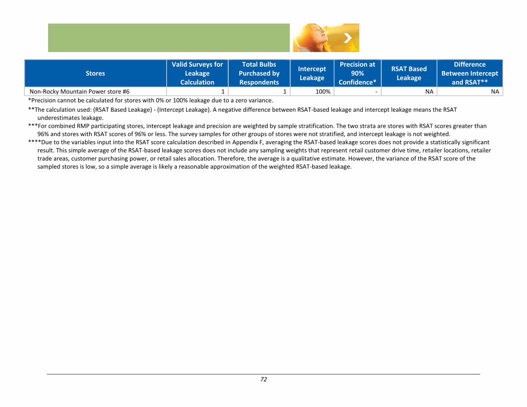
72
Stores Valid Surveys for
Leakage Calculation
Total Bulbs Purchased by Respondents
Intercept Leakage
Precision at 90%
Confidence*
RSAT Based Leakage
Difference Between Intercept
and RSAT** Non-Rocky Mountain Power store #6 1 1 100% - NA NA
*Precision cannot be calculated for stores with 0% or 100% leakage due to a zero variance.
**The calculation used: (RSAT Based Leakage) - (Intercept Leakage). A negative difference between RSAT-based leakage and intercept leakage means the RSAT underestimates leakage.
***For combined RMP participating stores, intercept leakage and precision are weighted by sample stratification. The two strata are stores with RSAT scores greater than 96% and stores with RSAT scores of 96% or less. The survey samples for other groups of stores were not stratified, and intercept leakage is not weighted.
****Due to the variables input into the RSAT score calculation described in Appendix F, averaging the RSAT-based leakage scores does not provide a statistically significant result. This simple average of the RSAT-based leakage scores does not include any sampling weights that represent retail customer drive time, retailer locations, retailer trade areas, customer purchasing power, or retail sales allocation. Therefore, the average is a qualitative estimate. However, the variance of the RSAT score of the sampled stores is low, so a simple average is likely a reasonable approximation of the weighted RSAT-based leakage.
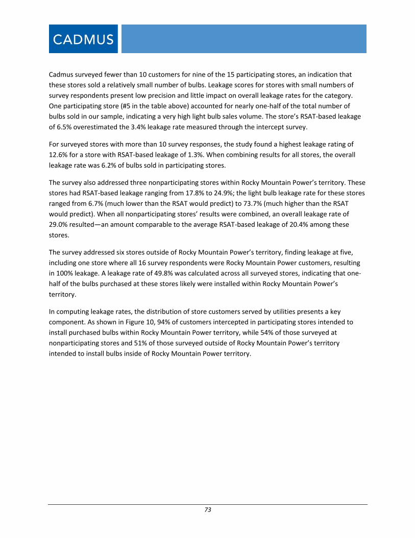
73
Cadmus surveyed fewer than 10 customers for nine of the 15 participating stores, an indication that
these stores sold a relatively small number of bulbs. Leakage scores for stores with small numbers of
survey respondents present low precision and little impact on overall leakage rates for the category.
One participating store (#5 in the table above) accounted for nearly one-half of the total number of
bulbs sold in our sample, indicating a very high light bulb sales volume. The store’s RSAT-based leakage
of 6.5% overestimated the 3.4% leakage rate measured through the intercept survey.
For surveyed stores with more than 10 survey responses, the study found a highest leakage rating of
12.6% for a store with RSAT-based leakage of 1.3%. When combining results for all stores, the overall
leakage rate was 6.2% of bulbs sold in participating stores.
The survey also addressed three nonparticipating stores within Rocky Mountain Power’s territory. These
stores had RSAT-based leakage ranging from 17.8% to 24.9%; the light bulb leakage rate for these stores
ranged from 6.7% (much lower than the RSAT would predict) to 73.7% (much higher than the RSAT
would predict). When all nonparticipating stores’ results were combined, an overall leakage rate of
29.0% resulted—an amount comparable to the average RSAT-based leakage of 20.4% among these
stores.
The survey addressed six stores outside of Rocky Mountain Power’s territory, finding leakage at five,
including one store where all 16 survey respondents were Rocky Mountain Power customers, resulting
in 100% leakage. A leakage rate of 49.8% was calculated across all surveyed stores, indicating that one-
half of the bulbs purchased at these stores likely were installed within Rocky Mountain Power’s
territory.
In computing leakage rates, the distribution of store customers served by utilities presents a key
component. As shown in Figure 10, 94% of customers intercepted in participating stores intended to
install purchased bulbs within Rocky Mountain Power territory, while 54% of those surveyed at
nonparticipating stores and 51% of those surveyed outside of Rocky Mountain Power’s territory
intended to install bulbs inside of Rocky Mountain Power territory.
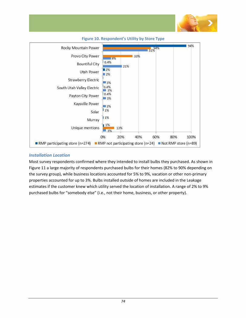
74
Figure 10. Respondent’s Utility by Store Type
Installation Location
Most survey respondents confirmed where they intended to install bulbs they purchased. As shown in
Figure 11 a large majority of respondents purchased bulbs for their homes (82% to 90% depending on
the survey group), while business locations accounted for 5% to 9%, vacation or other non-primary
properties accounted for up to 3%. Bulbs installed outside of homes are included in the Leakage
estimates if the customer knew which utility served the location of installation. A range of 2% to 9%
purchased bulbs for “somebody else” (i.e., not their home, business, or other property).
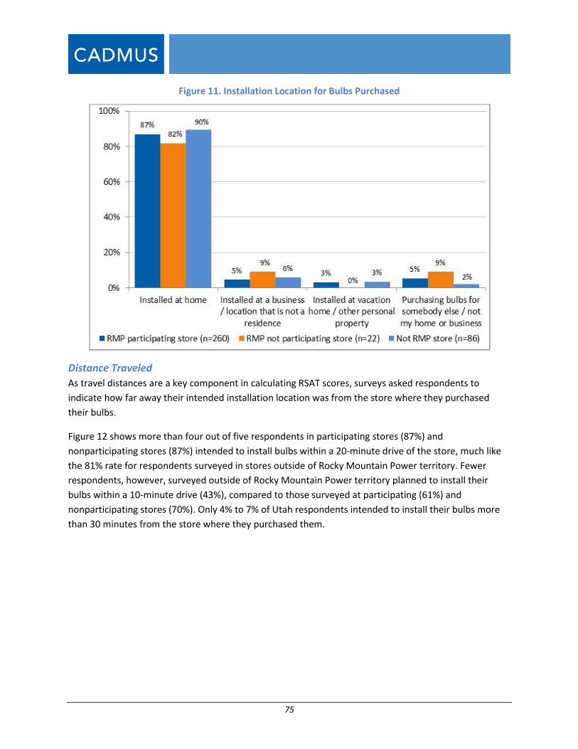
75
Figure 11. Installation Location for Bulbs Purchased
Distance Traveled
As travel distances are a key component in calculating RSAT scores, surveys asked respondents to
indicate how far away their intended installation location was from the store where they purchased
their bulbs.
Figure 12 shows more than four out of five respondents in participating stores (87%) and
nonparticipating stores (87%) intended to install bulbs within a 20-minute drive of the store, much like
the 81% rate for respondents surveyed in stores outside of Rocky Mountain Power territory. Fewer
respondents, however, surveyed outside of Rocky Mountain Power territory planned to install their
bulbs within a 10-minute drive (43%), compared to those surveyed at participating (61%) and
nonparticipating stores (70%). Only 4% to 7% of Utah respondents intended to install their bulbs more
than 30 minutes from the store where they purchased them.
76
Figure 12. Distance from Store to Installation Location
Purchase Quantities
Figure 13 shows the distribution of total bulbs (all types) purchased by survey respondents. Customers
surveyed in all three store types purchased similar numbers of bulbs, with nearly one-half (42% to 50%
per group) purchasing one or two bulbs and about one-third (29% to 31%) buying at least six bulbs. For
participating stores, customers purchased a mean number of 4.9 bulbs, with a median of 4.0 bulbs. For
stores outside of Rocky Mountain Power’s territory, customers purchased a mean of 5.4 bulbs and a
median of 3.0 bulbs. For nonparticipating stores, customers purchased a mean of 4.9 bulbs, with a
median of 2.0 bulbs.31
31 One survey respondent purchased six 24-packs of infrared heat lamp bulbs (i.e., 144 bulbs in total), saying
they were “for pets.” Though the figure includes this respondent Cadmus withheld this response from
calculation of the mean and median bulbs purchased by respondents in nonparticipating stores. Had the
outlier been included, the mean number of bulbs purchased for this group would have been 11, with a median
of three.
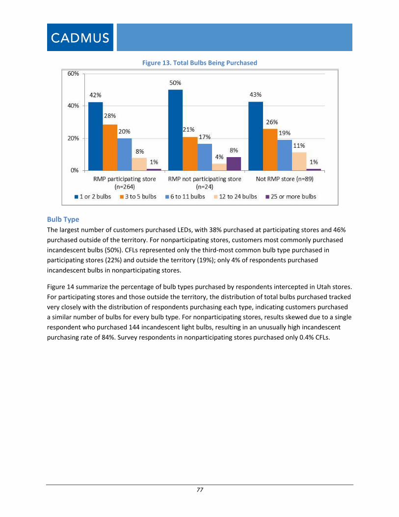
77
Figure 13. Total Bulbs Being Purchased
Bulb Type
The largest number of customers purchased LEDs, with 38% purchased at participating stores and 46%
purchased outside of the territory. For nonparticipating stores, customers most commonly purchased
incandescent bulbs (50%). CFLs represented only the third-most common bulb type purchased in
participating stores (22%) and outside the territory (19%); only 4% of respondents purchased
incandescent bulbs in nonparticipating stores.
Figure 14 summarize the percentage of bulb types purchased by respondents intercepted in Utah stores.
For participating stores and those outside the territory, the distribution of total bulbs purchased tracked
very closely with the distribution of respondents purchasing each type, indicating customers purchased
a similar number of bulbs for every bulb type. For nonparticipating stores, results skewed due to a single
respondent who purchased 144 incandescent light bulbs, resulting in an unusually high incandescent
purchasing rate of 84%. Survey respondents in nonparticipating stores purchased only 0.4% CFLs.
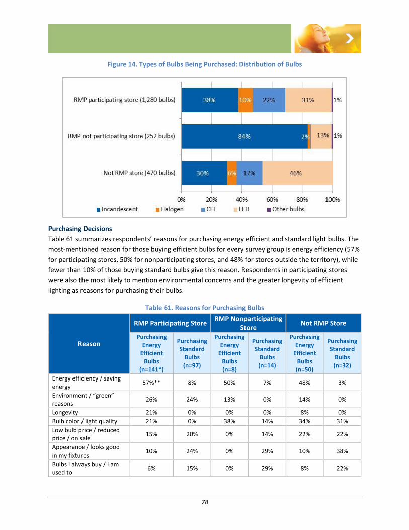
78
Figure 14. Types of Bulbs Being Purchased: Distribution of Bulbs
Purchasing Decisions
Table 61 summarizes respondents’ reasons for purchasing energy efficient and standard light bulbs. The
most-mentioned reason for those buying efficient bulbs for every survey group is energy efficiency (57%
for participating stores, 50% for nonparticipating stores, and 48% for stores outside the territory), while
fewer than 10% of those buying standard bulbs give this reason. Respondents in participating stores
were also the most likely to mention environmental concerns and the greater longevity of efficient
lighting as reasons for purchasing their bulbs.
Table 61. Reasons for Purchasing Bulbs
Reason
RMP Participating Store RMP Nonparticipating
Store Not RMP Store
Purchasing Energy
Efficient Bulbs
(n=141*)
Purchasing Standard
Bulbs (n=97)
Purchasing Energy
Efficient Bulbs (n=8)
Purchasing Standard
Bulbs (n=14)
Purchasing Energy
Efficient Bulbs (n=50)
Purchasing Standard
Bulbs (n=32)
Energy efficiency / saving energy
57%** 8% 50% 7% 48% 3%
Environment / “green” reasons
26% 24% 13% 0% 14% 0%
Longevity 21% 0% 0% 0% 8% 0%
Bulb color / light quality 21% 0% 38% 14% 34% 31%
Low bulb price / reduced price / on sale
15% 20% 0% 14% 22% 22%
Appearance / looks good in my fixtures
10% 24% 0% 29% 10% 38%
Bulbs I always buy / I am used to
6% 15% 0% 29% 8% 22%
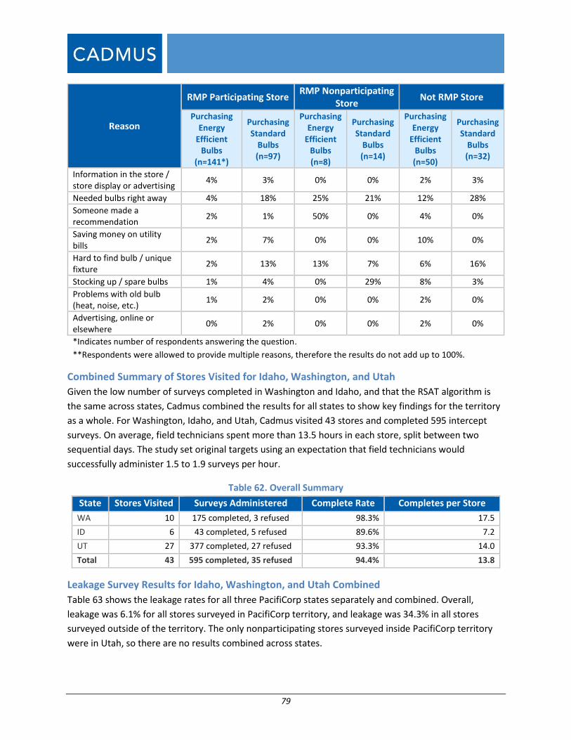
79
Reason
RMP Participating Store RMP Nonparticipating
Store Not RMP Store
Purchasing Energy
Efficient Bulbs
(n=141*)
Purchasing Standard
Bulbs (n=97)
Purchasing Energy
Efficient Bulbs (n=8)
Purchasing Standard
Bulbs (n=14)
Purchasing Energy
Efficient Bulbs (n=50)
Purchasing Standard
Bulbs (n=32)
Information in the store / store display or advertising
4% 3% 0% 0% 2% 3%
Needed bulbs right away 4% 18% 25% 21% 12% 28%
Someone made a recommendation
2% 1% 50% 0% 4% 0%
Saving money on utility bills
2% 7% 0% 0% 10% 0%
Hard to find bulb / unique fixture
2% 13% 13% 7% 6% 16%
Stocking up / spare bulbs 1% 4% 0% 29% 8% 3%
Problems with old bulb (heat, noise, etc.)
1% 2% 0% 0% 2% 0%
Advertising, online or elsewhere
0% 2% 0% 0% 2% 0%
*Indicates number of respondents answering the question.
**Respondents were allowed to provide multiple reasons, therefore the results do not add up to 100%.
Combined Summary of Stores Visited for Idaho, Washington, and Utah
Given the low number of surveys completed in Washington and Idaho, and that the RSAT algorithm is
the same across states, Cadmus combined the results for all states to show key findings for the territory
as a whole. For Washington, Idaho, and Utah, Cadmus visited 43 stores and completed 595 intercept
surveys. On average, field technicians spent more than 13.5 hours in each store, split between two
sequential days. The study set original targets using an expectation that field technicians would
successfully administer 1.5 to 1.9 surveys per hour.
Table 62. Overall Summary
State Stores Visited Surveys Administered Complete Rate Completes per Store
WA 10 175 completed, 3 refused 98.3% 17.5
ID 6 43 completed, 5 refused 89.6% 7.2
UT 27 377 completed, 27 refused 93.3% 14.0
Total 43 595 completed, 35 refused 94.4% 13.8
Leakage Survey Results for Idaho, Washington, and Utah Combined
Table 63 shows the leakage rates for all three PacifiCorp states separately and combined. Overall,
leakage was 6.1% for all stores surveyed in PacifiCorp territory, and leakage was 34.3% in all stores
surveyed outside of the territory. The only nonparticipating stores surveyed inside PacifiCorp territory
were in Utah, so there are no results combined across states.
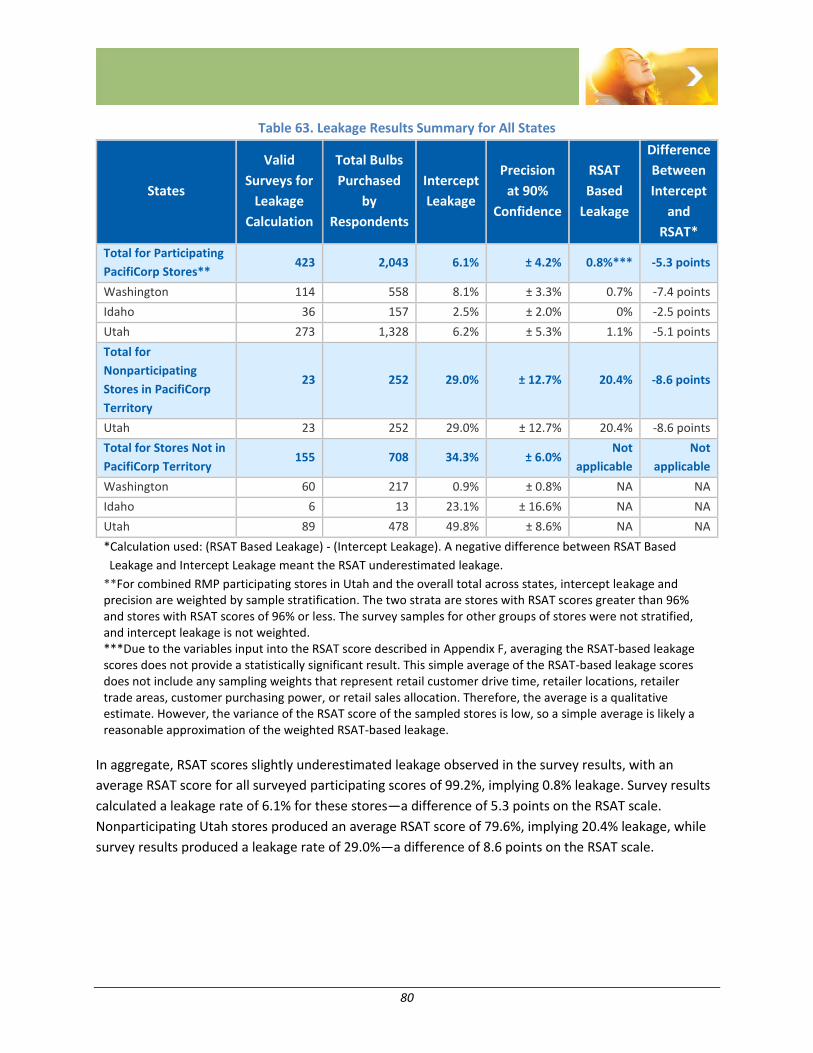
80
Table 63. Leakage Results Summary for All States
States
Valid
Surveys for
Leakage
Calculation
Total Bulbs
Purchased
by
Respondents
Intercept
Leakage
Precision
at 90%
Confidence
RSAT
Based
Leakage
Difference
Between
Intercept
and
RSAT*
Total for Participating
PacifiCorp Stores** 423 2,043 6.1% ± 4.2% 0.8%*** -5.3 points
Washington 114 558 8.1% ± 3.3% 0.7% -7.4 points
Idaho 36 157 2.5% ± 2.0% 0% -2.5 points
Utah 273 1,328 6.2% ± 5.3% 1.1% -5.1 points
Total for
Nonparticipating
Stores in PacifiCorp
Territory
23 252 29.0% ± 12.7% 20.4% -8.6 points
Utah 23 252 29.0% ± 12.7% 20.4% -8.6 points
Total for Stores Not in
PacifiCorp Territory 155 708 34.3% ± 6.0%
Not
applicable
Not
applicable
Washington 60 217 0.9% ± 0.8% NA NA
Idaho 6 13 23.1% ± 16.6% NA NA
Utah 89 478 49.8% ± 8.6% NA NA
*Calculation used: (RSAT Based Leakage) - (Intercept Leakage). A negative difference between RSAT Based
Leakage and Intercept Leakage meant the RSAT underestimated leakage.
**For combined RMP participating stores in Utah and the overall total across states, intercept leakage and precision are weighted by sample stratification. The two strata are stores with RSAT scores greater than 96% and stores with RSAT scores of 96% or less. The survey samples for other groups of stores were not stratified, and intercept leakage is not weighted. ***Due to the variables input into the RSAT score described in Appendix F, averaging the RSAT-based leakage scores does not provide a statistically significant result. This simple average of the RSAT-based leakage scores does not include any sampling weights that represent retail customer drive time, retailer locations, retailer trade areas, customer purchasing power, or retail sales allocation. Therefore, the average is a qualitative estimate. However, the variance of the RSAT score of the sampled stores is low, so a simple average is likely a reasonable approximation of the weighted RSAT-based leakage.
In aggregate, RSAT scores slightly underestimated leakage observed in the survey results, with an
average RSAT score for all surveyed participating scores of 99.2%, implying 0.8% leakage. Survey results
calculated a leakage rate of 6.1% for these stores—a difference of 5.3 points on the RSAT scale.
Nonparticipating Utah stores produced an average RSAT score of 79.6%, implying 20.4% leakage, while
survey results produced a leakage rate of 29.0%—a difference of 8.6 points on the RSAT scale.

81
Leakage Survey Results by Store Size
Cadmus categorized stores as “big box32” stores or “other stores,” enabling leakage result comparisons
between the two types. There is only one big box store in PacifiCorp’s Idaho territory, which we were
not allowed to visit; and all big box stores in Washington were participating stores in PacifiCorp’s
territory. All Utah big box stores were participating stores in PacifiCorp’s territory, but both store types
were surveyed among those outside PacifiCorp’s territory and among participating stores within the
territory. Overall, Cadmus interviewed 57% (n=601) of survey respondents in big box stores, with these
surveys accounting for 56% (n=3,003) of the total bulbs purchased by all respondents. Table 64 shows
big box stores usually exhibited leakage rates that were slightly higher than other stores, though
comparisons within states are not statistically significant.
Table 64. Leakage Results by Size of Store
States
Big Box Stores* Other Stores**
Valid
Surveys
for
Leakage
Calculation
Total
Bulbs
Purchased
Intercept
Leakage
Valid
Surveys for
Leakage
Calculation
Total
Bulbs
Purchased
Intercept
Leakage
Total for Participating
PacifiCorp Stores*** 291 1,447 7.7% 132 596 3.2%
Washington 72 287 11.5% 42 271 4.4%
Idaho 0 0 NA 36 157 2.5%
Utah 219 1,160 6.6% 54 168 3.9%
Total for
Nonparticipating Stores
in PacifiCorp Territory
0 0 NA 23 252 29.0%
Utah 0 0 NA 23 252 29.0%
Total for Stores Not in
PacifiCorp Territory 51 247 52.2% 104 461 24.7%
Washington 0 0 NA 60 217 0.9%
Idaho 0 0 NA 6 13 23.1%
Utah 51 247 52.2% 38 231 47.2%
*Twelve big box stores total: nine in Utah, three in Washington, zero in Idaho. **Twenty-seven other stores total: 15 in Utah, six in Washington, six in Idaho. ***For combined RMP participating stores in Utah and the overall total across states, intercept leakage and precision are weighted by sample stratification. The two strata are stores with RSAT scores greater than 96% and stores with RSAT scores of 96% or less. The survey samples for other groups of stores were not stratified, and intercept leakage is not weighted.
32 Large retail chains such as Home Depot, Lowe’s, Walmart, Target, Sutherland’s, and Big Lots.
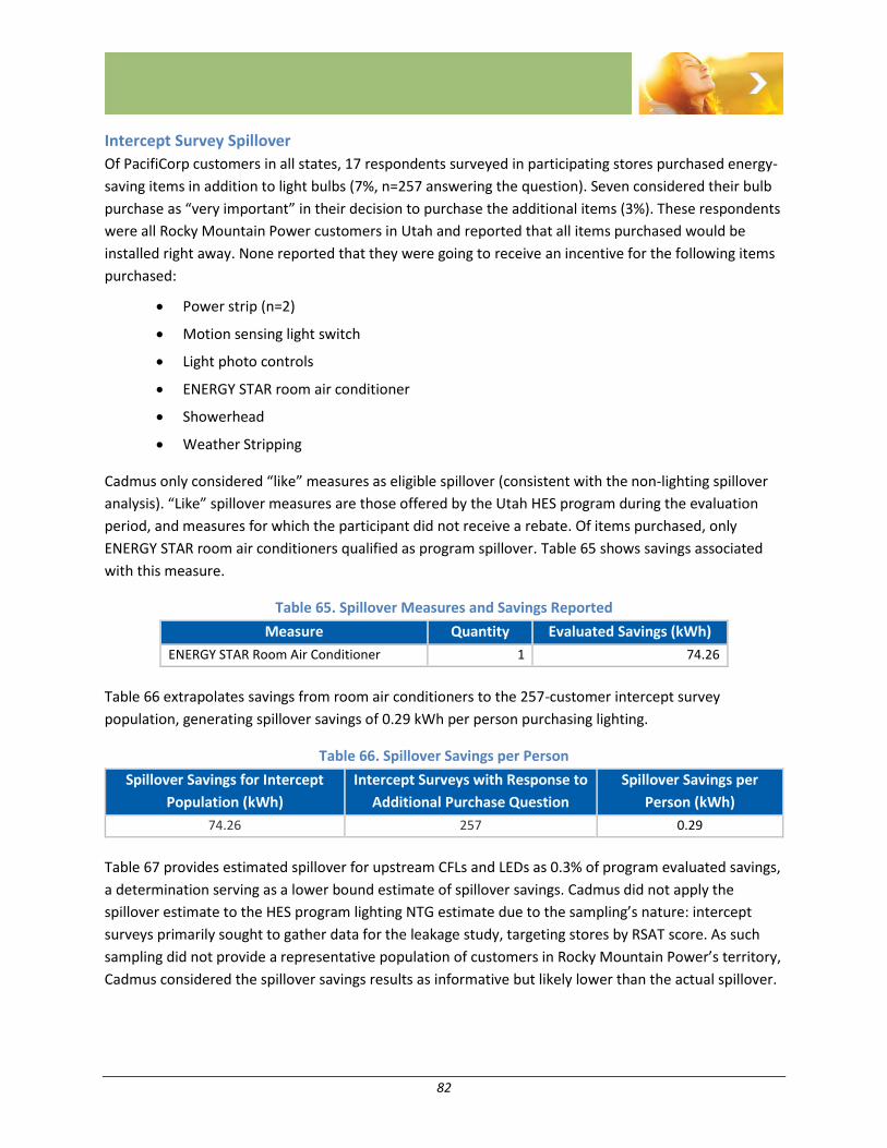
82
Intercept Survey Spillover
Of PacifiCorp customers in all states, 17 respondents surveyed in participating stores purchased energy-
saving items in addition to light bulbs (7%, n=257 answering the question). Seven considered their bulb
purchase as “very important” in their decision to purchase the additional items (3%). These respondents
were all Rocky Mountain Power customers in Utah and reported that all items purchased would be
installed right away. None reported that they were going to receive an incentive for the following items
purchased:
Power strip (n=2)
Motion sensing light switch
Light photo controls
ENERGY STAR room air conditioner
Showerhead
Weather Stripping
Cadmus only considered “like” measures as eligible spillover (consistent with the non-lighting spillover
analysis). “Like” spillover measures are those offered by the Utah HES program during the evaluation
period, and measures for which the participant did not receive a rebate. Of items purchased, only
ENERGY STAR room air conditioners qualified as program spillover. Table 65 shows savings associated
with this measure.
Table 65. Spillover Measures and Savings Reported
Measure Quantity Evaluated Savings (kWh)
ENERGY STAR Room Air Conditioner 1 74.26
Table 66 extrapolates savings from room air conditioners to the 257-customer intercept survey
population, generating spillover savings of 0.29 kWh per person purchasing lighting.
Table 66. Spillover Savings per Person
Spillover Savings for Intercept
Population (kWh)
Intercept Surveys with Response to
Additional Purchase Question
Spillover Savings per
Person (kWh)
74.26 257 0.29
Table 67 provides estimated spillover for upstream CFLs and LEDs as 0.3% of program evaluated savings,
a determination serving as a lower bound estimate of spillover savings. Cadmus did not apply the
spillover estimate to the HES program lighting NTG estimate due to the sampling’s nature: intercept
surveys primarily sought to gather data for the leakage study, targeting stores by RSAT score. As such
sampling did not provide a representative population of customers in Rocky Mountain Power’s territory,
Cadmus considered the spillover savings results as informative but likely lower than the actual spillover.
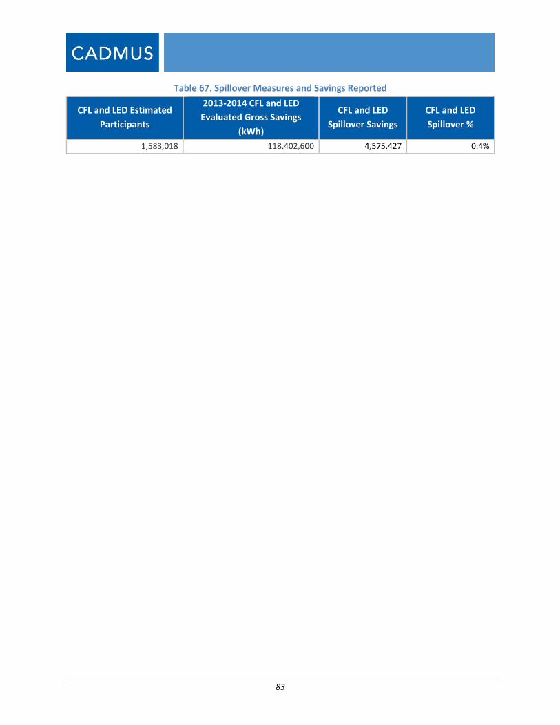
83
Table 67. Spillover Measures and Savings Reported
CFL and LED Estimated
Participants
2013-2014 CFL and LED
Evaluated Gross Savings
(kWh)
CFL and LED
Spillover Savings
CFL and LED
Spillover %
1,583,018 118,402,600 4,575,427 0.4%
84
Process Evaluation
This section describes the detailed findings of Cadmus’ process evaluation of the HES program. These
findings draw upon analysis of data collected through program staff interviews, a participant survey, the
general population survey, and secondary research. In conducting the evaluation, Cadmus focused on
assessing the following:
The delivery structure’s and implementation strategy’s effectiveness;
Marketing approaches;
Customer satisfaction; and
Internal and external communication channels.
Table 68 outlines the primary research questions.
Table 68. Research Areas
Research
Areas Researchable Questions and Topics
Program Status How did the program perform in 2013–2014, and what opportunities and challenges do
program staff foresee for future program years?
Satisfaction How satisfied are customers with their CFLs/LEDs or incented non-lighting measures? Why?
Awareness
Is the general population of customers aware of Rocky Mountain Power programs? If so,
how did they learn about the programs? How did non-lighting participants learn about the
HES program?
Motivations What actions have customers taken to save energy, and what motivated them to purchase
a CFL, LED, or non-lighting measure?
Demographics How do awareness/activities/behaviors vary by demographic characteristics?
Methodology Cadmus conducted the following process evaluation research:
Program and marketing materials review
Utility and administrator staff interviews
General population survey
Non-lighting participant survey
Program Materials Review
The program materials review focused on critical program documents, including past evaluation reports,
the program logic model, and program marketing and communications materials developed to promote
HES program participation and to educate target audiences in Utah about program offerings. In addition
to the materials review, Cadmus discussed marketing effectiveness with program stakeholders and
considered their insights when analyzing participant survey findings and industry best practices.

85
The materials review included the following:
In assessing program progress and analyzing trends across program years, Cadmus considered
the findings and conclusions from the Rocky Mountain Power 2011–2012 Utah Residential Home
Energy Savings Evaluation and the Rocky Mountain Power 2009-2010 Utah Residential Home
Energy Savings Evaluation.
Cadmus reviewed the HES program logic model to reflect the 2013–2014 program processes
(see Appendix H) and, based on information gathered through program staff interviews,
determined that the logic model accurately reflected current program operations.
Cadmus reviewed Rocky Mountain Power’s marketing plans and online materials and compared
their messages to the challenges and motivations described by customers, seeking to assess
whether the program’s marketing has been appropriately targeted. Cadmus reviewed the HES
program marketing strategy, executional plans, and online (website) and social media elements.
Utility and Administrator Staff Interviews
Cadmus developed stakeholder interview guides and collected information about key topics from
program management staff. The evaluation involved two interviews: one with two program staff at
Rocky Mountain Power; and one with two program staff at CLEAResult (the program administrator),
which oversees the HES program in five PacifiCorp service territory states.
The interviews covered the following topics:
Program status and delivery processes;
Program design and implementation changes;
Marketing and outreach tactics; and
Barriers and areas for improvement.
Cadmus conducted the interviews by telephone and contacted the interviewees via e-mail with follow-
up questions or clarification requests.
Participant Survey
Cadmus conducted a telephone survey with non-lighting participating customers, designing the survey
instrument to collect data regarding the following process topics:
Program process. Details to inform the following performance indicators:
o Effectiveness of the program processes;
o Program awareness;
o Participation motivations and barriers;
o Customer satisfaction; and
o Program strengths and/or areas for improvement.
Customer information. Demographic information and household statistics.

86
General Population Survey
Cadmus conducted a telephone survey with customers regarding lighting purchases, designing the
survey instrument to collect data regarding the following process topics:
Program process. Details to inform the following performance indicators:
o Upstream lighting rebate awareness;
o Lighting purchase decisions and barriers to purchasing energy-efficient lighting;
o Customer satisfaction with products purchased; and
Customer information. Demographic information and household statistics.
Program Implementation and Delivery Drawing on stakeholder interviews and participant survey data, this section discusses HES program
implementation and delivery.
Program Overview
Through the 2013-2014 HES program, Rocky Mountain Power provided cash incentives to residential
customers for purchases of energy-efficient products, home improvements, and heating and cooling
equipment and services. Under the program, customers could install multiple measures to create
customized efficiency portfolios, thus lowering their utility bills. Rocky Mountain Power encouraged all
its residential customers, including non-homeowners and owners of multifamily buildings and
manufactured homes, to participate in the program.
During the evaluation period, Rocky Mountain Power in Utah offered energy efficiency measures in two
primary categories, based on the program’s two delivery channels: lighting and non-lighting. Only
internal program staff referred to these two categories; the company did not market the program this
way to customers. The lighting component used an upstream incentive mechanism that may not be
apparent to customers, whereas the non-lighting component operated using a mail-in or online (for
select measures) incentive approach, which requires participant awareness and action. All incentives
were prescriptive. In 2015, program staff expanded the program by adding a mail-order energy
efficiency kit option.
Tariff Changes
Each year, Rocky Mountain Power files program modifications (i.e., tariff changes) with the Utah Public
Utilities Commission. Two key program changes during 2013 and 2014 included the addition of direct-
install duct sealing for customers in manufactured homes and a realignment of incentives for
comprehensive whole-home upgrades. Program staff also made minor adjustments to the efficiency
level required for several measures eligible for program incentives, such as clothes washers,
refrigerators, and freezers.
87
Delivery Structure and Processes
Per program staff, the HES program saw minimal changes to its customer delivery method since 2009.
Program staff coordinated with participating distributors, retailers, and trade allies to deliver the
program’s different components. For most program-qualifying measures customers received cash-back
incentives. For qualifying light bulbs, program staff paid incentives directly to manufacturers, who
provided high efficiency bulbs to retailers at a discount; retailers, sales associates, and trade allies
supported the program by encouraging customers to purchase higher-efficiency equipment that
qualifies for an incentive.
Data Tracking
The program administrator reported that data tracking systems in place met, and in some cases
exceeded, its needs, allowing meaningful use of data collected. Program administrator staff reported
entering program data into their Key What You See (KWYS) system, a Microsoft Access-based tool. Some
KWYS data were transferred into a Salesforce database. Weekly aggregation of participant databases
allowed the program administrator to monitor incentives paid and goal achieved, and each month the
program administrator provided Rocky Mountain Power with a report which allows program staff to
evaluate and diagnose the causes of program activity changes, enabling program delivery adjustments, if
needed.
In 2013, the program administrator began transitioning rebate data entry to a third-party vendor,
National Business Systems (NBS), because the program administrator reported dissatisfaction with the
previous vendor. The transition began with the program administrator providing NBS access to one
measure at a time until it could prove it could operate under all program rules. Program staff reported
the transition a success.
The program processed upstream lighting invoices through a system called Sprocket. The program
administrator received invoices from the manufacturer, verified the information’s accuracy, and entered
data into a tool. The data flowed through a validation and quality control (QC) process before entering
Sprocket.
While upstream lighting data tracking effectively served the program administrator’s and Rocky
Mountain Power’s needs and expectations, Cadmus experienced some challenges when using the data
for evaluation purposes. Specifically, significant issues emerged when matching lighting tracking data
(Sprocket) to price scheduling data for linking bulb prices and incentives to lighting products sold. These
data issues included the following:
1. Inconsistent bulb types for each SKU.
2. Inconsistent use of SKUs vs. model numbers to track products.
3. Inconsistent use of “posted,” “reconciled,” and “posted-reconciled” tags to track the final
quantities of bulbs sold through the program.
4. Very limited tracking of product merchandising and promotional events.
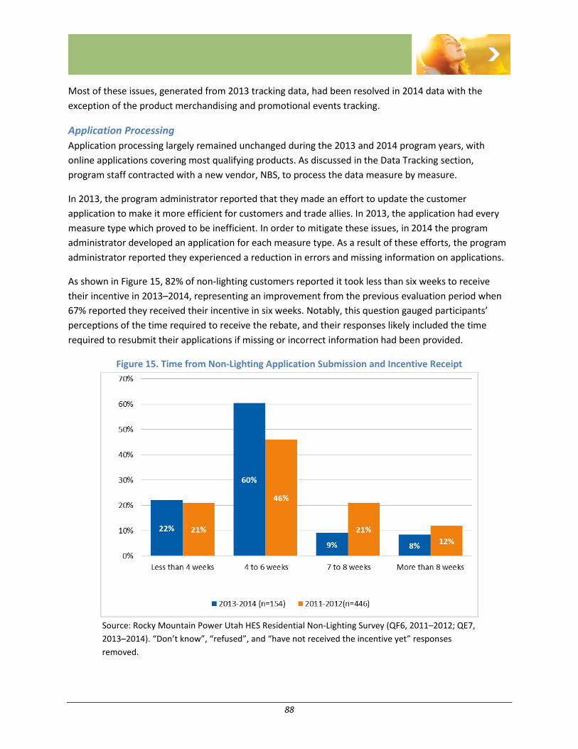
88
Most of these issues, generated from 2013 tracking data, had been resolved in 2014 data with the
exception of the product merchandising and promotional events tracking.
Application Processing
Application processing largely remained unchanged during the 2013 and 2014 program years, with
online applications covering most qualifying products. As discussed in the Data Tracking section,
program staff contracted with a new vendor, NBS, to process the data measure by measure.
In 2013, the program administrator reported that they made an effort to update the customer
application to make it more efficient for customers and trade allies. In 2013, the application had every
measure type which proved to be inefficient. In order to mitigate these issues, in 2014 the program
administrator developed an application for each measure type. As a result of these efforts, the program
administrator reported they experienced a reduction in errors and missing information on applications.
As shown in Figure 15, 82% of non-lighting customers reported it took less than six weeks to receive
their incentive in 2013–2014, representing an improvement from the previous evaluation period when
67% reported they received their incentive in six weeks. Notably, this question gauged participants’
perceptions of the time required to receive the rebate, and their responses likely included the time
required to resubmit their applications if missing or incorrect information had been provided.
Figure 15. Time from Non-Lighting Application Submission and Incentive Receipt
Source: Rocky Mountain Power Utah HES Residential Non-Lighting Survey (QF6, 2011–2012; QE7,
2013–2014). “Don’t know”, “refused”, and “have not received the incentive yet” responses
removed.
89
Cadmus also analyzed participants’ reported wait times by measure. For example, in 2013–2014, 85% of
insulation participants reported receiving their incentives within six weeks, compared to 59% in 2011–
2012. Similarly, 80% of window participants reported receiving their incentives within six weeks,
compared to 67% in 2011–2012.33 Only duct sealing and insulation exhibited poor performance, with
42% of customers reported a wait of seven or more weeks (n=12).
Eighty-eighty percent of non-lighting customers expressed satisfaction with the time required to receive
the incentive. Among the 12% of customers who expressed dissatisfaction (19 total customers), four
reported having to resubmit paperwork.
Overall, 64% of non-lighting customers expressed high satisfaction rates (“very satisfied”) with the
application process. Thirty-two percent said they were somewhat satisfied, 1% said they were not very
satisfied, and 2% said they were not at all satisfied. Dissatisfied customers offered the following reasons
for their discontent:
“The application process was easy, but they kept asking questions of the contract process they
didn’t need [to].”
“I have not received the incentive check yet.”
“We never got the rebate.”/“I didn’t receive the incentive.”
“The length, and the frustration, and the rejection of a completely filled out application.”/
“It was too much to do.”
“It didn’t do what it was supposed to do.”
“Filling out the application was too complicated.”
“[Our contractor] tried to get us to pay because they can’t work with [Rocky Mountain Power]
and couldn’t get the paperwork they needed.”
Retailers and Trade Allies
Program staff continued using the tiered account management system, developed in earlier program
years to streamline the process of working with trade allies and retailers: the program administrator
divides trade allies into two tiers for internal tracking purposes only. Program staff estimated that Tier 1
trade allies accounted for 80% of the program savings and tended to conduct the most work with
customers. Tier 2 trade allies do fewer projects per year than Tier 1 trade allies.
The program administrator regularly (at least three times per year) offered training to distributors,
retailers, and their associates. Program administrator staff reported the regular training necessary due
to the following reasons:
Addressing rapid turnover in the industry;
Keeping trade allies abreast of program changes; and
33 Statistically significant change (p-value <0.10).
90
Working toward the program administrators’ goal to use trade ally education to reduce the
number of applications with errors.
For example, at the beginning of heating season, the program administrator contacted retailer account
managers to discuss products in demand in that season. For the upstream lighting component, the
program administrator focused on delivering training to Home Depot and Lowes to educate each sales
associate about the program and to train them on how to sell energy-efficient products to a customer.
The program administrator reported the trainings resulted in increased retailer participation between
2013 and 2014, especially during the summer cooling season.
The program administrator also reported focusing its Tier 1 trade ally training and communication
efforts on technology and tariff changes. For example, following the 2014 state tariffs update in Utah,
the program administrator conducted trainings with trade allies to ensure they understood the changes
and their implications. The efforts sought to aid in seamless tariff implementation without failures in
customer service.
Marketing
Approach
To operate as efficiently as possible, program staff reported streamlining the Utah marketing and
outreach approaches to maximize the delivery of direct energy-saving opportunities. According to the
2014 Marketing Plan, this strategy resulted in a shift of resources toward targeted marketing and away
from mass marketing. Staff used bill inserts, social media, sell sheets, and website features that
employed tailored messages.
For 2014, the following five key strategies emerged:
1. Focus on priority measures during key seasonal selling windows (e.g., heating season, cooling
season, and lighting season).
2. Shift the marketing mix to more cost-effective, flexible, and measureable delivery.
3. Simplify and enhance the customer experience to increase participation.
4. Streamline basic program processes, leverage opportunities, and track results to reduce cost of
marketing
5. Strategically support unplanned opportunities.
Materials and Website Review
The 2014 Marketing Communications Plan developed by the program administrator clearly outlines a
broad marketing strategy for the HES program. While the plan effectively maps out major strategic focus
areas, it lacks details regarding the tactics program staff intended to use and over what time period to
execute the marketing strategy.
Primarily, the plan identifies a need to shift most program marketing and application processes to an
online format. By the end of 2014, the program website reflected a simple, easy-to-understand
91
structure (by measure category), allowing customers to apply online and to check an application’s status
for most measure categories. These changes, meant to simplify the process for customers, likely
contributed to program satisfaction discussed in this report. The website, however, lacks language to
motivate a customer to participate (i.e., a “call to action”).
Effectiveness
The program administrator tracks marketing effectiveness on a limited basis, with the marketing team
tracking click-through statistics for the program website. In 2015, the team began tracking time spent on
the website, how customers reached the website, and materials they viewed.
The program administrator staff also noted that the guerrilla (marketing in an unconventional way) tool
kit developed for lighting and appliances effectively engaged retailers. The tool kit provided talking
points that educated retail employees about the business case for energy efficiency and its contribution
to retailer profits.
Program Challenges and Successes HES program staff reported the program faced a primary challenge: communicating tariff changes to
trade allies. For example, when the Utah tariff changed, trade allies had difficulty understanding the
tariff, its changes, and the way it was written. The program administrator mitigated confusion over
future tariff changes by providing education and training opportunities to trade allies once a tariff
changed.
In 2013, increased U.S. DOE and the ENERGY STAR program standards for clothes washers and
refrigerators eliminated a majority of program-qualifying models, causing challenges with retailers.
Program staff reported this change stressed relationships with retailers, but offered staff an opportunity
to contact and begin a dialogue with retail partners.
Program staff reported that the program’s requirement of using an eligible contractor to allow the
customer to qualify for rebates presented challenges in 2013 and 2014 as many trade allies did not
know about the program and had not yet become a part of the trade ally network. Some customers
expressed frustration that their upgrades did not qualify as they did not use an eligible contractor. To
mitigate this, program staff began reaching out to new trade allies, encouraging them to enroll with the
program within 90 days of a customer submitting a rebate application to permit the customer’s
application processing.
The Utah market’s rural customer population also presented significant challenges. As rural Rocky
Mountain Power customers did not frequent a participating retailer’s store, where they would have
seen program advertisements or would have been able to purchase some HES products, program staff
began rethinking their marketing and outreach approach with these customers. These conversations
ultimately led to the development of the energy efficiency kits, introduced in 2015 (and hence not
covered by this evaluation).
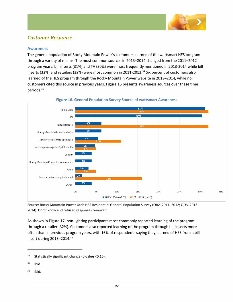
92
Customer Response
Awareness
The general population of Rocky Mountain Power’s customers learned of the wattsmart HES program
through a variety of means. The most common sources in 2013–2014 changed from the 2011–2012
program years: bill inserts (31%) and TV (30%) were most frequently mentioned in 2013-2014 while bill
inserts (32%) and retailers (32%) were most common in 2011-2012.34 Six percent of customers also
learned of the HES program through the Rocky Mountain Power website in 2013–2014, while no
customers cited this source in previous years. Figure 16 presents awareness sources over these time
periods.35
Figure 16. General Population Survey Source of wattsmart Awareness
Source: Rocky Mountain Power Utah HES Residential General Population Survey (QB2, 2011–2012; QD3, 2013–
2014). Don’t know and refused responses removed.
As shown in Figure 17, non-lighting participants most commonly reported learning of the program
through a retailer (32%). Customers also reported learning of the program through bill inserts more
often than in previous program years, with 16% of respondents saying they learned of HES from a bill
insert during 2013–2014.36
34 Statistically significant change (p-value <0.10).
35 Ibid.
36 Ibid.
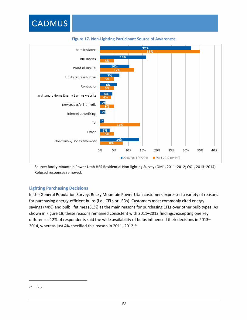
93
Figure 17. Non-Lighting Participant Source of Awareness
Source: Rocky Mountain Power Utah HES Residential Non-lighting Survey (QM1, 2011–2012; QC1, 2013–2014).
Refused responses removed.
Lighting Purchasing Decisions
In the General Population Survey, Rocky Mountain Power Utah customers expressed a variety of reasons
for purchasing energy-efficient bulbs (i.e., CFLs or LEDs). Customers most commonly cited energy
savings (44%) and bulb lifetimes (31%) as the main reasons for purchasing CFLs over other bulb types. As
shown in Figure 18, these reasons remained consistent with 2011–2012 findings, excepting one key
difference: 12% of respondents said the wide availability of bulbs influenced their decisions in 2013–
2014, whereas just 4% specified this reason in 2011–2012.37
37 Ibid.
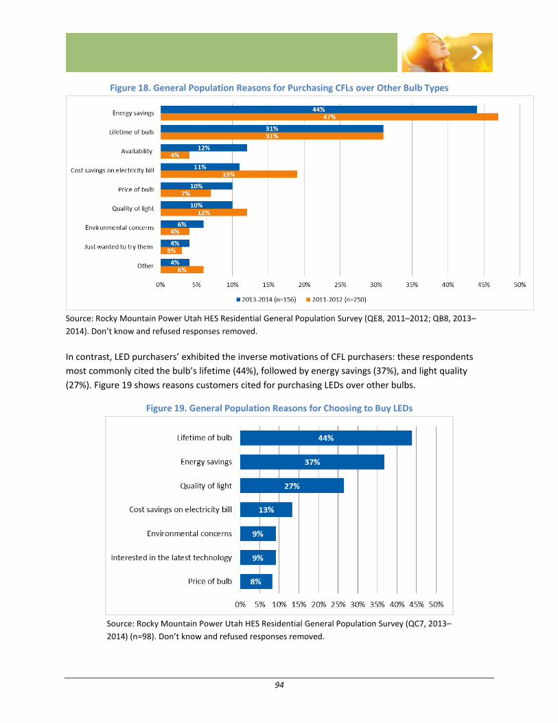
94
Figure 18. General Population Reasons for Purchasing CFLs over Other Bulb Types
Source: Rocky Mountain Power Utah HES Residential General Population Survey (QE8, 2011–2012; QB8, 2013–
2014). Don’t know and refused responses removed.
In contrast, LED purchasers’ exhibited the inverse motivations of CFL purchasers: these respondents
most commonly cited the bulb’s lifetime (44%), followed by energy savings (37%), and light quality
(27%). Figure 19 shows reasons customers cited for purchasing LEDs over other bulbs.
Figure 19. General Population Reasons for Choosing to Buy LEDs
Source: Rocky Mountain Power Utah HES Residential General Population Survey (QC7, 2013–
2014) (n=98). Don’t know and refused responses removed.
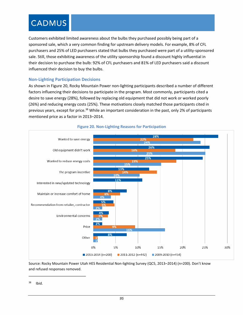
95
Customers exhibited limited awareness about the bulbs they purchased possibly being part of a
sponsored sale, which a very common finding for upstream delivery models. For example, 8% of CFL
purchasers and 25% of LED purchasers stated that bulbs they purchased were part of a utility-sponsored
sale. Still, those exhibiting awareness of the utility sponsorship found a discount highly influential in
their decision to purchase the bulb: 92% of CFL purchasers and 81% of LED purchasers said a discount
influenced their decision to buy the bulbs.
Non-Lighting Participation Decisions
As shown in Figure 20, Rocky Mountain Power non-lighting participants described a number of different
factors influencing their decisions to participate in the program. Most commonly, participants cited a
desire to save energy (28%), followed by replacing old equipment that did not work or worked poorly
(26%) and reducing energy costs (25%). These motivations closely matched those participants cited in
previous years, except for price.38 While an important consideration in the past, only 2% of participants
mentioned price as a factor in 2013–2014.
Figure 20. Non-Lighting Reasons for Participation
Source: Rocky Mountain Power Utah HES Residential Non-lighting Survey (QC5, 2013–2014) (n=200). Don’t know
and refused responses removed.
38 Ibid.

96
Satisfaction
Lighting
Customers differed somewhat in their satisfaction levels with products they purchased, depending on
whether they purchased CFLs or LEDs. Consistent with prior years, 50% of CFL customers said they were
very satisfied with their purchase and 36% said they were somewhat satisfied, as shown in Figure 21.
Figure 21. General Population CFL Satisfaction
Source: Rocky Mountain Power Utah HES Residential General Population Survey (QG1, 2011–2012,
QB15, 2013–2014). Don’t know and refused responses removed.
Customers purchasing LEDs expressed higher satisfaction, with 76% very satisfied and 19% somewhat
satisfied. As shown in Figure 22, LED satisfaction levels appear to have increased over the evaluation
periods.
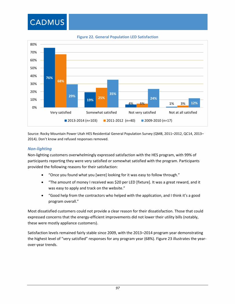
97
Figure 22. General Population LED Satisfaction
Source: Rocky Mountain Power Utah HES Residential General Population Survey (QM8, 2011–2012, QC14, 2013–
2014). Don’t know and refused responses removed.
Non-lighting
Non-lighting customers overwhelmingly expressed satisfaction with the HES program, with 99% of
participants reporting they were very satisfied or somewhat satisfied with the program. Participants
provided the following reasons for their satisfaction:
“Once you found what you [were] looking for it was easy to follow through.”
“The amount of money I received was $20 per LED [fixture]. It was a great reward, and it
was easy to apply and track on the website.”
“Good help from the contractors who helped with the application, and I think it’s a good
program overall.”
Most dissatisfied customers could not provide a clear reason for their dissatisfaction. Those that could
expressed concerns that the energy-efficient improvements did not lower their utility bills (notably,
these were mostly appliance customers).
Satisfaction levels remained fairly stable since 2009, with the 2013–2014 program year demonstrating
the highest level of “very satisfied” responses for any program year (68%). Figure 23 illustrates the year-
over-year trends.
76%
19%4% 1%
68%
25%
5% 3%
29%35%
24%12%
0%
10%
20%
30%
40%
50%
60%
70%
80%
Very satisfied Somewhat satisfied Not very satisfied Not at all satisfied
2013-2014 (n=103) 2011-2012 (n=40) 2009-2010 (n=17)
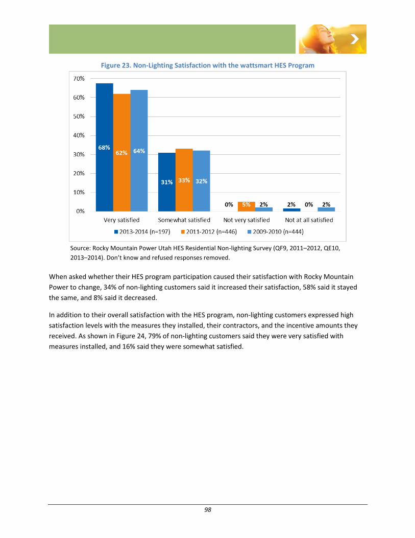
98
Figure 23. Non-Lighting Satisfaction with the wattsmart HES Program
Source: Rocky Mountain Power Utah HES Residential Non-lighting Survey (QF9, 2011–2012, QE10,
2013–2014). Don’t know and refused responses removed.
When asked whether their HES program participation caused their satisfaction with Rocky Mountain
Power to change, 34% of non-lighting customers said it increased their satisfaction, 58% said it stayed
the same, and 8% said it decreased.
In addition to their overall satisfaction with the HES program, non-lighting customers expressed high
satisfaction levels with the measures they installed, their contractors, and the incentive amounts they
received. As shown in Figure 24, 79% of non-lighting customers said they were very satisfied with
measures installed, and 16% said they were somewhat satisfied.

99
Figure 24. Non-Lighting Satisfaction with Measures, Contractors, Incentive Amounts
Source: Rocky Mountain Power Utah HES Residential Non-lighting Survey (QE1, E3, E6 2013–2014).
Don’t know and refused responses removed.
About three-quarters of participants hired contractors to install measures for which they received
program incentives; 82% of these participants reported being very satisfied with their contractors and
16% were somewhat satisfied. A slightly smaller share of participants expressed satisfaction with the
incentive amounts they received, with 64% reporting they were very satisfied with the incentive
amounts. An additional 31% said they were somewhat satisfied, and just 6% said they were not very or
not at all satisfied.
Non-lighting customers also found the HES program incentive application easy to fill out, with 71% of
respondents reporting it very easy to fill out, 25% reporting it somewhat, 1% reporting it not very easy,
and 3% reporting it not at all easy. Participants experiencing difficulty with filling out the application
noted the following challenges:
“I just wasn’t able to navigate it very well.”
“It was repetitive.”
“Because I had to get copies of forms for every [online] window.”
“It was too long and requested info that no user would ever have on hand; I had to go back
to the dealer for more information.”
Customer Demographics
As shown in Figure 25, most of the general population surveyed and non-lighting participants lived in
single-family homes, with a small percentage of customers residing in condominiums, townhomes,
apartments, or mobile homes.
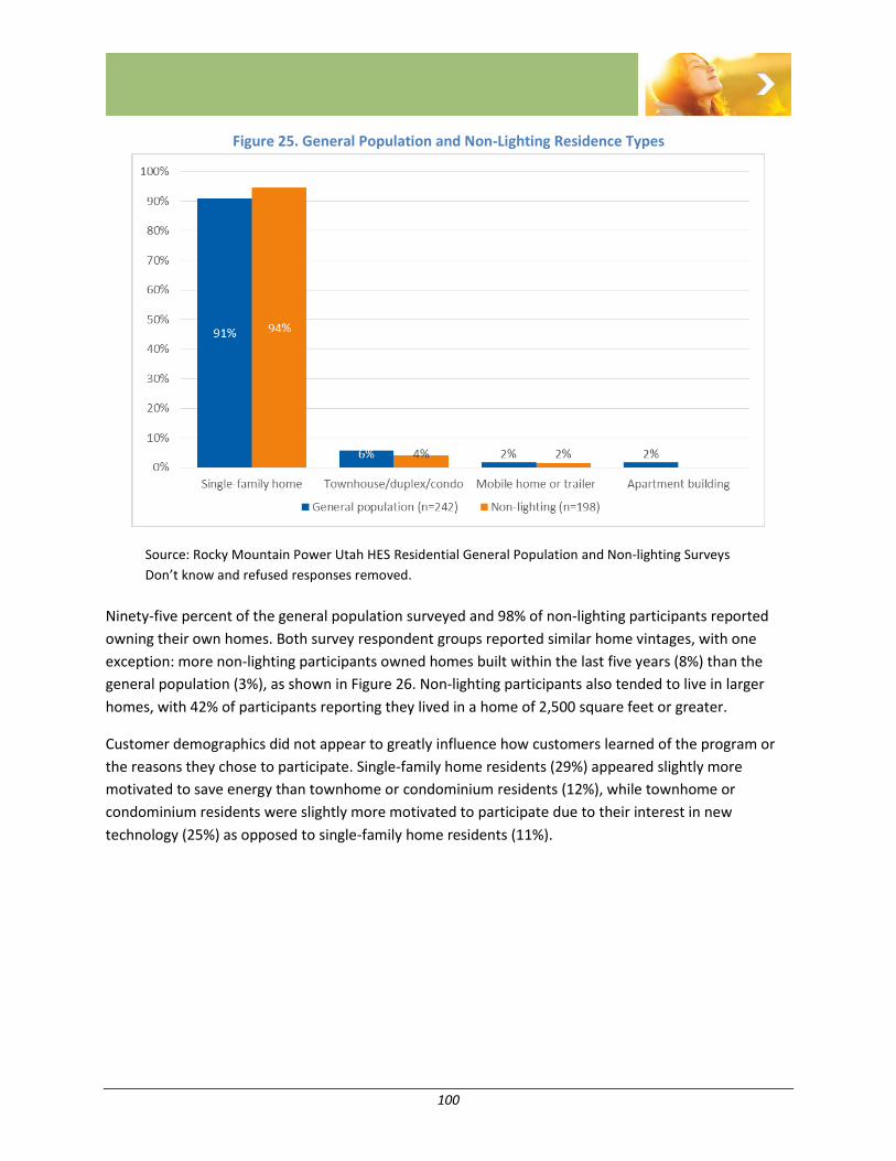
100
Figure 25. General Population and Non-Lighting Residence Types
Source: Rocky Mountain Power Utah HES Residential General Population and Non-lighting Surveys
Don’t know and refused responses removed.
Ninety-five percent of the general population surveyed and 98% of non-lighting participants reported
owning their own homes. Both survey respondent groups reported similar home vintages, with one
exception: more non-lighting participants owned homes built within the last five years (8%) than the
general population (3%), as shown in Figure 26. Non-lighting participants also tended to live in larger
homes, with 42% of participants reporting they lived in a home of 2,500 square feet or greater.
Customer demographics did not appear to greatly influence how customers learned of the program or
the reasons they chose to participate. Single-family home residents (29%) appeared slightly more
motivated to save energy than townhome or condominium residents (12%), while townhome or
condominium residents were slightly more motivated to participate due to their interest in new
technology (25%) as opposed to single-family home residents (11%).
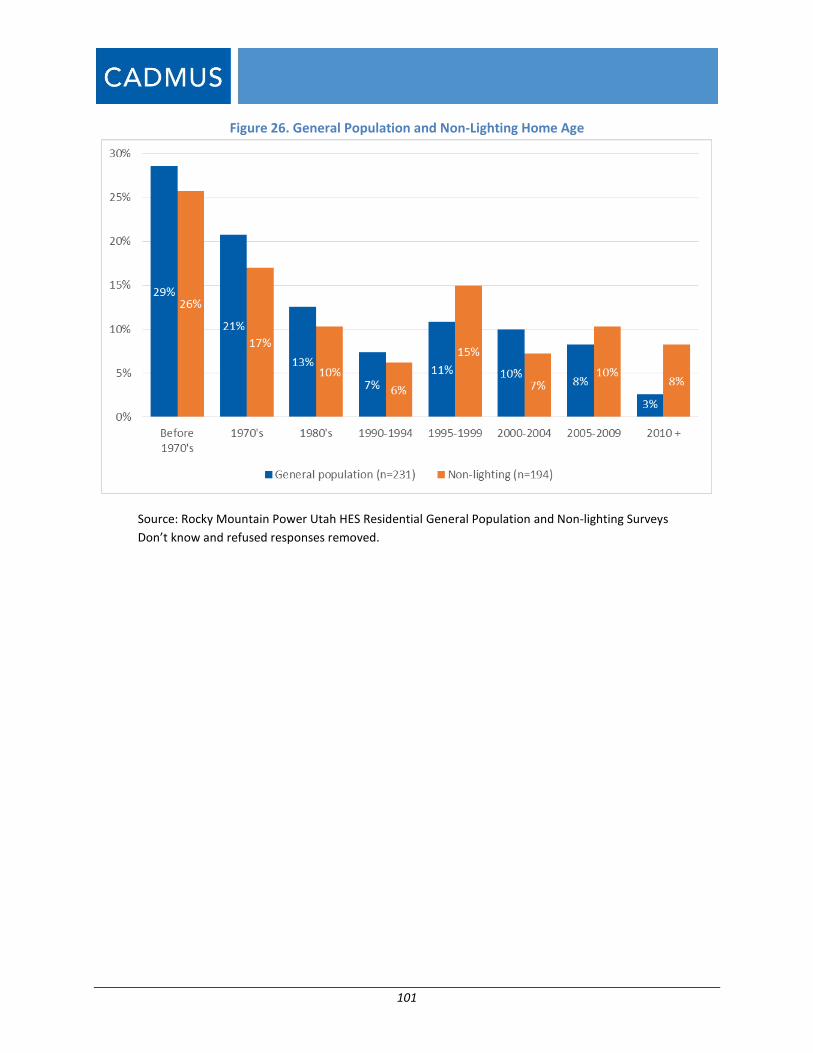
101
Figure 26. General Population and Non-Lighting Home Age
Source: Rocky Mountain Power Utah HES Residential General Population and Non-lighting Surveys
Don’t know and refused responses removed.
102
Cost-Effectiveness
In assessing HES program cost-effectiveness, Cadmus analyzed program costs and benefits from five
different perspectives, using Cadmus’ DSM Portfolio Pro39 model. The California Standard Practice
Manual for assessing DSM program cost-effectiveness describes the benefit/cost ratios Cadmus used for
the following five tests:
1. PacifiCorp Total Resource Cost (PTRC) Test: This test examined program benefits and costs from
Rocky Mountain Power’s and Rocky Mountain Power customers’ perspectives (combined). On
the benefit side, it included avoided energy costs, capacity costs, and line losses, plus a 10%
adder to reflect non-quantified benefits. On the cost side, it included costs incurred by both the
utility and participants.
2. Total Resource Cost (TRC) Test: This test also examined program benefits and costs from Rocky
Mountain Power’s and Rocky Mountain Power customers’ perspectives (combined). On the
benefit side, it included avoided energy costs, capacity costs, and line losses. On the cost side, it
included costs incurred by both the utility and participants.
3. Utility Cost Test (UCT): This test examined program benefits and costs solely from Rocky
Mountain Power’s perspective. The benefits included avoided energy, capacity costs, and line
losses. Costs included program administration, implementation, and incentive costs associated
with program funding.
4. Ratepayer Impact Measure (RIM) Test: All ratepayers (participants and nonparticipants) may
experience rate increases designed to recover lost revenues. The benefits included avoided
energy costs, capacity costs, and line losses. Costs included all Rocky Mountain Power program
costs and lost revenues.
5. Participant Cost Test (PCT): From this perspective, program benefits included bill reductions and
incentives received. Costs included a measure’s incremental cost (compared to the baseline
measures), plus installation costs incurred by the customer.
Table 69 summarizes the five tests’ components.
39 DSM Portfolio Pro has been independently reviewed by various utilities, their consultants, and a number of
regulatory bodies, including the Iowa Utility Board, the Public Service Commission of New York, the Colorado
Public Utilities Commission, and the Nevada Public Utilities Commission.
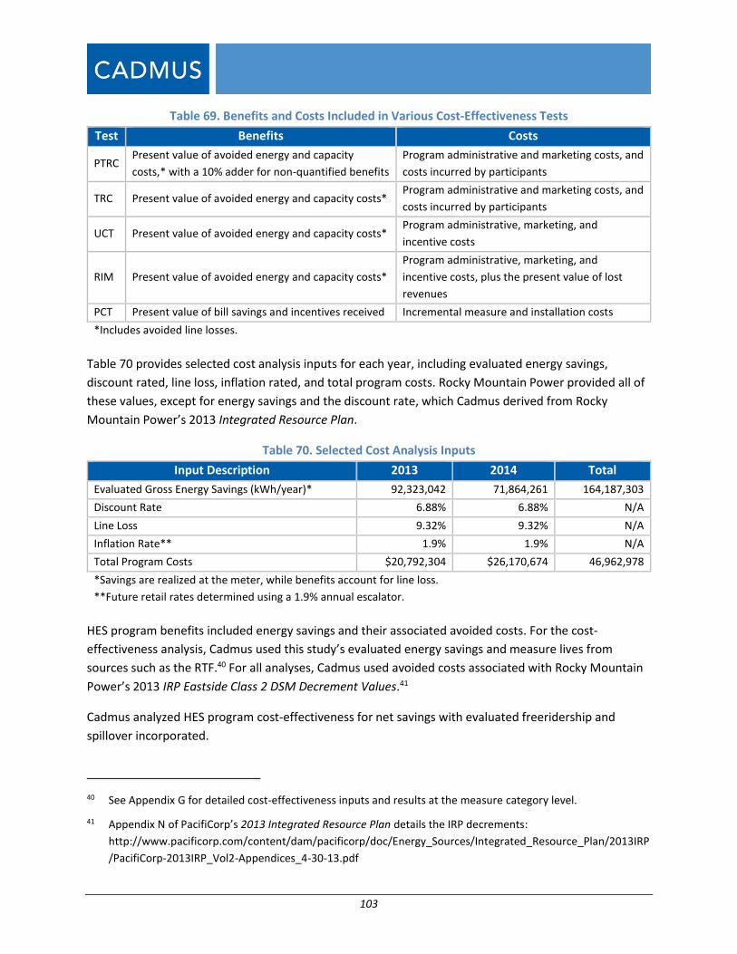
103
Table 69. Benefits and Costs Included in Various Cost-Effectiveness Tests
Test Benefits Costs
PTRC Present value of avoided energy and capacity
costs,* with a 10% adder for non-quantified benefits
Program administrative and marketing costs, and
costs incurred by participants
TRC Present value of avoided energy and capacity costs* Program administrative and marketing costs, and
costs incurred by participants
UCT Present value of avoided energy and capacity costs* Program administrative, marketing, and
incentive costs
RIM Present value of avoided energy and capacity costs*
Program administrative, marketing, and
incentive costs, plus the present value of lost
revenues
PCT Present value of bill savings and incentives received Incremental measure and installation costs
*Includes avoided line losses.
Table 70 provides selected cost analysis inputs for each year, including evaluated energy savings,
discount rated, line loss, inflation rated, and total program costs. Rocky Mountain Power provided all of
these values, except for energy savings and the discount rate, which Cadmus derived from Rocky
Mountain Power’s 2013 Integrated Resource Plan.
Table 70. Selected Cost Analysis Inputs
Input Description 2013 2014 Total
Evaluated Gross Energy Savings (kWh/year)* 92,323,042 71,864,261 164,187,303
Discount Rate 6.88% 6.88% N/A
Line Loss 9.32% 9.32% N/A
Inflation Rate** 1.9% 1.9% N/A
Total Program Costs $20,792,304 $26,170,674 46,962,978
*Savings are realized at the meter, while benefits account for line loss.
**Future retail rates determined using a 1.9% annual escalator.
HES program benefits included energy savings and their associated avoided costs. For the cost-
effectiveness analysis, Cadmus used this study’s evaluated energy savings and measure lives from
sources such as the RTF.40 For all analyses, Cadmus used avoided costs associated with Rocky Mountain
Power’s 2013 IRP Eastside Class 2 DSM Decrement Values.41
Cadmus analyzed HES program cost-effectiveness for net savings with evaluated freeridership and
spillover incorporated.
40 See Appendix G for detailed cost-effectiveness inputs and results at the measure category level.
41 Appendix N of PacifiCorp’s 2013 Integrated Resource Plan details the IRP decrements:
http://www.pacificorp.com/content/dam/pacificorp/doc/Energy_Sources/Integrated_Resource_Plan/2013IRP
/PacifiCorp-2013IRP_Vol2-Appendices_4-30-13.pdf
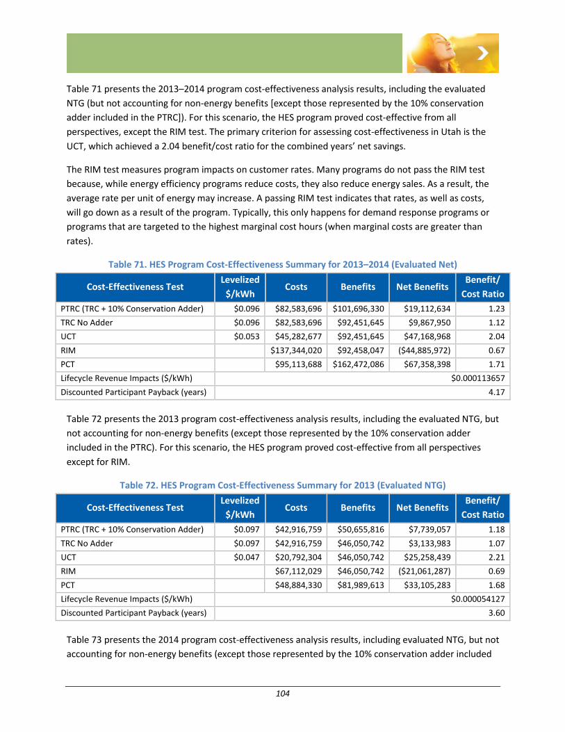
104
Table 71 presents the 2013–2014 program cost-effectiveness analysis results, including the evaluated
NTG (but not accounting for non-energy benefits [except those represented by the 10% conservation
adder included in the PTRC]). For this scenario, the HES program proved cost-effective from all
perspectives, except the RIM test. The primary criterion for assessing cost-effectiveness in Utah is the
UCT, which achieved a 2.04 benefit/cost ratio for the combined years’ net savings.
The RIM test measures program impacts on customer rates. Many programs do not pass the RIM test
because, while energy efficiency programs reduce costs, they also reduce energy sales. As a result, the
average rate per unit of energy may increase. A passing RIM test indicates that rates, as well as costs,
will go down as a result of the program. Typically, this only happens for demand response programs or
programs that are targeted to the highest marginal cost hours (when marginal costs are greater than
rates).
Table 71. HES Program Cost-Effectiveness Summary for 2013–2014 (Evaluated Net)
Cost-Effectiveness Test Levelized
$/kWh Costs Benefits Net Benefits
Benefit/
Cost Ratio
PTRC (TRC + 10% Conservation Adder) $0.096 $82,583,696 $101,696,330 $19,112,634 1.23
TRC No Adder $0.096 $82,583,696 $92,451,645 $9,867,950 1.12
UCT $0.053 $45,282,677 $92,451,645 $47,168,968 2.04
RIM $137,344,020 $92,458,047 ($44,885,972) 0.67
PCT $95,113,688 $162,472,086 $67,358,398 1.71
Lifecycle Revenue Impacts ($/kWh) $0.000113657
Discounted Participant Payback (years) 4.17
Table 72 presents the 2013 program cost-effectiveness analysis results, including the evaluated NTG, but
not accounting for non-energy benefits (except those represented by the 10% conservation adder
included in the PTRC). For this scenario, the HES program proved cost-effective from all perspectives
except for RIM.
Table 72. HES Program Cost-Effectiveness Summary for 2013 (Evaluated NTG)
Cost-Effectiveness Test Levelized
$/kWh Costs Benefits Net Benefits
Benefit/
Cost Ratio
PTRC (TRC + 10% Conservation Adder) $0.097 $42,916,759 $50,655,816 $7,739,057 1.18
TRC No Adder $0.097 $42,916,759 $46,050,742 $3,133,983 1.07
UCT $0.047 $20,792,304 $46,050,742 $25,258,439 2.21
RIM $67,112,029 $46,050,742 ($21,061,287) 0.69
PCT $48,884,330 $81,989,613 $33,105,283 1.68
Lifecycle Revenue Impacts ($/kWh) $0.000054127
Discounted Participant Payback (years) 3.60
Table 73 presents the 2014 program cost-effectiveness analysis results, including evaluated NTG, but not
accounting for non-energy benefits (except those represented by the 10% conservation adder included
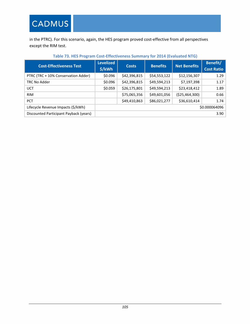
105
in the PTRC). For this scenario, again, the HES program proved cost-effective from all perspectives
except the RIM test.
Table 73. HES Program Cost-Effectiveness Summary for 2014 (Evaluated NTG)
Cost-Effectiveness Test Levelized
$/kWh Costs Benefits Net Benefits
Benefit/
Cost Ratio
PTRC (TRC + 10% Conservation Adder) $0.096 $42,396,815 $54,553,122 $12,156,307 1.29
TRC No Adder $0.096 $42,396,815 $49,594,213 $7,197,398 1.17
UCT $0.059 $26,175,801 $49,594,213 $23,418,412 1.89
RIM $75,065,356 $49,601,056 ($25,464,300) 0.66
PCT $49,410,863 $86,021,277 $36,610,414 1.74
Lifecycle Revenue Impacts ($/kWh) $0.000064096
Discounted Participant Payback (years) 3.90
106
Conclusions and Recommendations
Based on the findings previously presented, Cadmus offers the following conclusions and
recommendations.
Measure Categorization Some measure categories were assigned based on delivery channels rather than end uses (e.g., light
fixtures were assigned as appliances while in the downstream delivery channel). For cost-effectiveness
purposes, measure categories should be allocated by end use to ensure employing the most appropriate
load shape.
Recommendation
Assign measure categories by end use to ensure use of the most appropriate cost-effectiveness results.
Ensure consistent applications of measure categories in all data tracking and reporting efforts (including
annual reports, evaluations, and participant databases).
Upstream Lighting Tracking Database While Cadmus was able to match the quantities and savings in the lighting tracking database to annual
reports, the data proved challenging to use for evaluation purposes. Specifically, Cadmus encountered
difficulties in mapping the lighting tracking database to the price scheduling database.
The tracking database contained several inconsistences: bulb types were inconsistently defined for each
SKU; SKUs and model numbers were used interchangeably; and reconciled quantities were
inconsistently labeled. The program administrator also could not provide detailed tracking information
on product merchandising or promotional events. Data tracking, however, improved significantly
between 2013 and 2014. Many of the inconsistencies were changes due to manufacturers updating
descriptions between price schedules (the negotiated period for which prices and incentives are agreed
upon between manufacturers/retailers and the program implementer). The 2014 tracking data included
the schedule name in both the pricing data as well as the sales data, which improved the accuracy in
matching prices to sales rather than having to rely on inconsistent secondary descriptions. If the data
continues to be collected in the same way for 2015-2016 as it was in 2014, Cadmus will not face as many
challenges in the next evaluation.
Recommendation
Track all data in a consistent manner across each program period. This specifically includes
the following:
Provide consistently defined bulb types for each SKU;
Provide consistent SKUs or model numbers;
Provide tracking data with final and reconciled quantities; and
107
Track all product merchandising and promotional events (was not tracked in either 2013 or
2014).
Lighting Cross-Sector Sales Cadmus estimated that 3.9% of efficient bulbs purchased at retail store ultimately would be installed in
commercial applications, which is a similar result to findings in other jurisdictions that also implement
upstream lighting programs. Bulbs installed in commercial spaces produce more first-year savings than
bulbs installed in a residential space as commercial locations typically have a higher daily use of bulbs
than residential locations (i.e., higher HOU). Currently, Rocky Mountain Power does not account for
cross-sector sales from the upstream lighting incentives.
Recommendation
Other jurisdictions around the country increasingly have accommodated cross-sector sales factors in
calculating reported lighting savings. Cadmus recommends that Rocky Mountain Power explore
accounting for commercial installation of upstream bulbs in the reported savings.
Accounting for these installations can be complex due the nature of the split between residential and
nonresidential programs within the wattsmart portfolio. One option would be to calculate savings values
for each bulb, accounting for the different HOUs for residential and nonresidential installations
weighted by the cross-sector sales factor. This option would also require calculating a lower measure life
to account for commercial bulbs burning out faster. Finally, Rocky Mountain Power would then need to
decide if all of the lighting savings from the program would fall under the residential wattsmart portfolio
or if some of the savings would be transferred onto the nonresidential side.
Nonparticipant Spillover Nonparticipant spillover results in energy savings caused by, but not rebated through, utilities’ demand-
side management activities. Effective program marketing and outreach generates program participation
and increases general energy efficiency awareness among customers. The cumulative effect of sustained
utility program marketing can affect customers’ perceptions of their energy usage and, in some cases,
motivate customers to take efficiency actions outside of the utility’s program.
Through responses to the general population survey, Cadmus estimated nonparticipant spillover as 1%
of HES program savings. Due to the introduction of this type of spillover to the evaluation, Cadmus did
not apply this adjustment.
Recommendation
Consider allowing nonparticipant spillover to be an integral component of NTG estimations for all
programs.
Lighting Leakage Through intercept surveys conducted with customers purchasing light bulbs at 15 participating retail
stores, Cadmus found that lighting leakage rates were an average of roughly 5.1 percentage points
108
higher than predicted by the RSAT, with a confidence level of 90% and precision of ± 5.3%, indicating
that the RSAT is performing well as a predictor of bulb leakage.
Cadmus estimated a leakage rate of 49.8% across all surveyed stores outside of (but bordering) Rocky
Mountain Power’s territory, indicating that one-half of the bulbs purchased at these stores likely were
installed within Rocky Mountain Power’s territory. These stores did not have RSAT scores to compare
against.
Customers were more likely to purchase CFLs and LEDs at participating stores (53% of bulbs purchased
were CFLs or LEDs) than at nonparticipating stores (13% of bulbs purchased were CFLs or LEDs) in Utah.
Recommendation
The RSAT allocation score is performing well in Utah. Rocky Mountain Power should continue using the
RSAT to determine which stores in its territory should be included as participating stores in the program.
Lighting Spillover This evaluation examined a portion of spillover found from the upstream lighting leakage survey through
store intercepts, however, it was not an exhaustive view of spillover since sufficient time could not pass
for customers to implement measures. Also, the store intercept sampling plan was primarily designed to
support the RSAT calculations, meaning that most sampled stores either were on the edges or outside of
Rocky Mountain Power’s territory. Therefore, the 0.4% spillover calculated is likely a low estimate and
further studies are needed to estimate lighting spillover.
Recommendation
Consider additional studies to quantify spillover (and potentially market transformation) for use in
lighting NTG calculations.
Customer Outreach Bill inserts and retailers constituted the most commonly cited program awareness sources for non-
lighting participants. While the program website was an influential source of general wattsmart
awareness for the general population, it did not serve as a main participation driver for the non-lighting
program.
Recommendation
Continue to pursue a multi-touch marketing strategy, using a mix of bill inserts and retailer/contractor
training. Given the large percentage of customers who learned of wattsmart offerings through bill
inserts, examine the proportion of customers selecting to receive online bills and ensure these online
channels proportionately advertise the programs with the messages that motivated customers to
participate: long-lasting products, saving energy, replacing equipment and reducing costs.
109
Application Processing Efforts to improve the ease of completing the non-lighting incentive application appear to have
succeeded: non-lighting participants reported faster incentive check processing times and relative ease
in filling out applications. Ninety-six percent of survey respondents found it very easy to fill out the
incentive application.
Despite these substantive improvements, participant-reported application processing times remained
lengthy for duct sealing and insulation customers and also attic, floor, and wall insulation, indicating
opportunities for improvements regarding specific measures.
Recommendation
Continue to review methods for simplifying the applications, particularly for duct sealing and insulation
applications which have been prone to greater data entry errors. Implement additional training for
HVAC and weatherization contractors to help mitigate this issue by reviewing the criteria required for a
complete application and how to best support a customer who chooses to fill out the application.
Explore making duct sealing and insulation an online application to reduce errors.
Satisfaction with Program Experience Customers generally expressed satisfaction with their program experiences, including high satisfaction
levels with contractors. While Cadmus was not able to verify the efficacy of the program administrator’s
efforts to reach out to non-registered contractors who worked with rebate-seeking participants, the
program’s efforts to mitigate contractor confusion regarding tariff changes appeared to support the
customers’ reported satisfaction.
Recommendation
Continue regular trainings with trade allies (e.g., distributors, retailers, sales associates, contractors),
updating them on tariff changes and, where appropriate, supporting them with sales and marketing
training. Analyze success of efforts to register non-registered contractors who worked with rebate
participants within 90 days to determine whether the additional outreach mitigated the number of
rejected applications due to non-qualified contractors.

110
Appendices
A separate volume contains the following appendices:
Appendix A. Survey and Data Collection Forms
Appendix B. Lighting Impacts
Appendix C. Billing Analysis
Appendix D. Self-Report NTG Methodology
Appendix E. Nonparticipant Spillover
Appendix F. Lighting Retailer Allocation Review
Appendix G. Measure Category Cost-Effectiveness
Appendix H. Logic Model

Appendix A. Survey Instruments and Data Collection Tools
Management Staff and Program Partner Interview Guide ........................................................................ A-1
Rebate Participant Survey .......................................................................................................................... A-5
Upstream Lighting Survey ........................................................................................................................ A-32
Lighting Leakage Survey ........................................................................................................................... A-57

Appendix A-1
PacifiCorp HES Program PM Staff Interview Guide PY 2013 - 2014
Name: Title: Interviewer: Date of Interview:
Introduction
The purpose of the interview is to explore your experience with the HES Program. We use input from a variety of staff involved with the program to describe how the program worked during 2013 and 2014, what made it successful, and where there may be opportunities for improvement. Please feel free to let me know if there are questions that may not apply to your role so that we can focus on the areas with which you have worked most closely.
Program Overview, Management Roles and Responsibilities:
1. To start, please tell me about your role and associated responsibilities with the HES Program.
a. How long have you been involved?
b. Who are the other key PacifiCorp staff involved in the 2013 and 2014 program period and what are their roles?
Program Goal and Objectives:
2. How would you describe the main objective of the 2013 and 2014 HES Program?
3. What were the savings and participation goals of the program for 2013 and 2014? How did the program do with respect to those goals?
4. Did the program have any informal or internal goals/Key Performance Indicators for this year, such as level of trade ally engagement, participant satisfaction, participation in certain regions, etc.?
a. How or why were these goals developed?

Appendix A-2
b. How did the program perform in terms of reaching the internal goals (for each state)?
5. Please walk me through how the program worked from a customer perspective. For example, how would a customer hear about the program, how would participation be initiated, and what steps would I go through as a customer? (for all delivery channels – upstream, rebate and kits).
6. How did this customer experience differ among the five states?
7. [If not covered above] Please tell me about how the program worked with trade allies. What types of trade allies did you work with? What are their roles and responsibilities?
Program Design:
Thank you. Now I’d like to ask you about the program design.
8. [If not answered above] Who is your target market for this program?
9. How well did the current program design meet customer needs? (Probe: measures, incentive levels, documentation required, etc.)
10. Were any major changes made to the program since 2012? (incentives, program components (kits), etc) [Probe: Simple Steps, kits]?
a. What was the reason kits were introduce to ID, CA and WA? Are there plans to provide the kits in UT and WY too?
b. Are the kits a standard set of measures or can customers choose which components they want? How is this tracked? [Cadmus will request the specifications for each kit item during a follow-up data request]
c. Were any changes made to the rebate application forms (recommendation from last evaluation)?
d. Have there been any tariff changes since 2012?
11. What worked well in the 2013-2014 period?
12. Conversely, what was not working as well as anticipated?

Appendix A-3
13. What barriers or challenges did the program face in 2013-2014? What was done/what is planned to address them?
14. What changes are planned or now in place for the HES program (by state)?
15. What was the program’s QA/QC process like in 2013-2014? Would you please describe that?
16. In your opinion, what other ways can the program design be improved? (Probe: What? Why?)
Program Marketing
17. [If not covered above] Please describe how the program was marketed (through the website, one-on-one outreach, through trade allies, etc.)?
18. Do you have a marketing plan from 2013-2014 you could share with me? What were the primary marketing activities during that time period?
a. Did all five states use the same marketing plan and tactics?
b. How did the messaging differ in the five states?
c. How much of the marketing is wattsmart vs program specific (HES)?
d. Who is the primary target audience for the program?
19. Did you track marketing effectiveness? What did you track?
a. What was the most effective marketing approach? (Why do you say this?)
Customer Experience:
20. Did you have a process by which you receive customer feedback about the program? (Probe: What is that process and how frequently does it happen, what happens to the information, if a response is required who does that?)
21. What feedback did you receive from customers about the program? What did they say? (Probe: incentive levels, timing for project approvals, incentive payments, satisfaction with studies, trade allies, etc.)
Appendix A-4
Trade Ally Experience:
22. How did the program recruit trade allies (contractors and retailers)?
23. Do you feel you had sufficient trade allies to support the program? Why or why not?
24. What barriers have the trade allies said they encounter with the program?
a. What steps have been taken to address these?
b. What remains to be done to remove these barriers?
25. What kind of training was required and/or offered for trade allies? How frequently and on what topics?
26. Did the program provide marketing resources or sales training to trade allies?
Data Tracking and Savings
27. Please tell us about program data tracking and reporting. How were rebate forms processed? (Probe: What systems did they use, how well did systems communicate, how did trade allies and other stakeholders submit information to the program?). Please describe for all delivery mechanisms (rebates, upstream, kits).
28. Did the data tracking systems in place meet your needs? Why or why not?
29. How were savings deemed for each program measure? How often were the unit energy savings values updated? [Cadmus will request unit energy saving calculators/assumptions during a follow-up data request]
Closing
30. Are there specific topics you are interested in learning more about from our evaluation this year?
31. For the purposes of our customer survey, what should we call the program? Will customers recognize Home Energy Savings, or should we use wattsmart/bewattsmart?
Thank you very much for your time today!
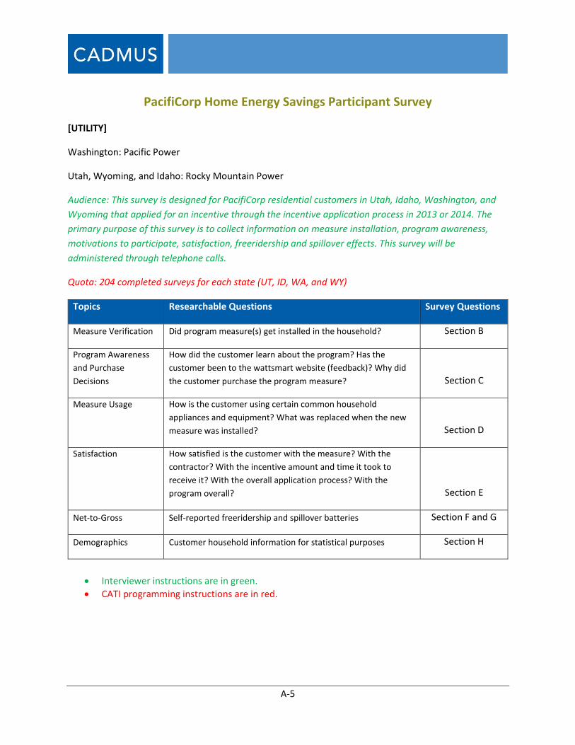
A-5
PacifiCorp Home Energy Savings Participant Survey
[UTILITY]
Washington: Pacific Power
Utah, Wyoming, and Idaho: Rocky Mountain Power
Audience: This survey is designed for PacifiCorp residential customers in Utah, Idaho, Washington, and
Wyoming that applied for an incentive through the incentive application process in 2013 or 2014. The
primary purpose of this survey is to collect information on measure installation, program awareness,
motivations to participate, satisfaction, freeridership and spillover effects. This survey will be
administered through telephone calls.
Quota: 204 completed surveys for each state (UT, ID, WA, and WY)
Topics Researchable Questions Survey Questions
Measure Verification Did program measure(s) get installed in the household? Section B
Program Awareness
and Purchase
Decisions
How did the customer learn about the program? Has the
customer been to the wattsmart website (feedback)? Why did
the customer purchase the program measure? Section C
Measure Usage How is the customer using certain common household
appliances and equipment? What was replaced when the new
measure was installed? Section D
Satisfaction How satisfied is the customer with the measure? With the
contractor? With the incentive amount and time it took to
receive it? With the overall application process? With the
program overall? Section E
Net-to-Gross Self-reported freeridership and spillover batteries Section F and G
Demographics Customer household information for statistical purposes Section H
Interviewer instructions are in green.
CATI programming instructions are in red.
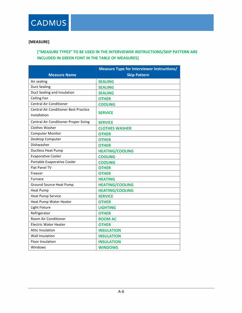
A-6
[MEASURE]
[“MEASURE TYPES” TO BE USED IN THE INTERVIEWER INSTRUCTIONS/SKIP PATTERN ARE
INCLUDED IN GREEN FONT IN THE TABLE OF MEASURES]
Measure Name
Measure Type for Interviewer Instructions/
Skip Pattern
Air sealing SEALING
Duct Sealing SEALING Duct Sealing and Insulation SEALING Ceiling Fan OTHER Central Air Conditioner COOLING Central Air Conditioner Best Practice
Installation SERVICE
Central Air Conditioner Proper Sizing SERVICE Clothes Washer CLOTHES WASHER Computer Monitor OTHER Desktop Computer OTHER Dishwasher OTHER Ductless Heat Pump HEATING/COOLING Evaporative Cooler COOLING Portable Evaporative Cooler COOLING Flat Panel TV OTHER
Freezer OTHER
Furnace HEATING
Ground Source Heat Pump HEATING/COOLING
Heat Pump HEATING/COOLING
Heat Pump Service SERVICE Heat Pump Water Heater OTHER Light Fixture LIGHTING
Refrigerator OTHER
Room Air Conditioner ROOM AC
Electric Water Heater OTHER
Attic Insulation INSULATION
Wall Insulation INSULATION
Floor Insulation INSULATION Windows WINDOWS
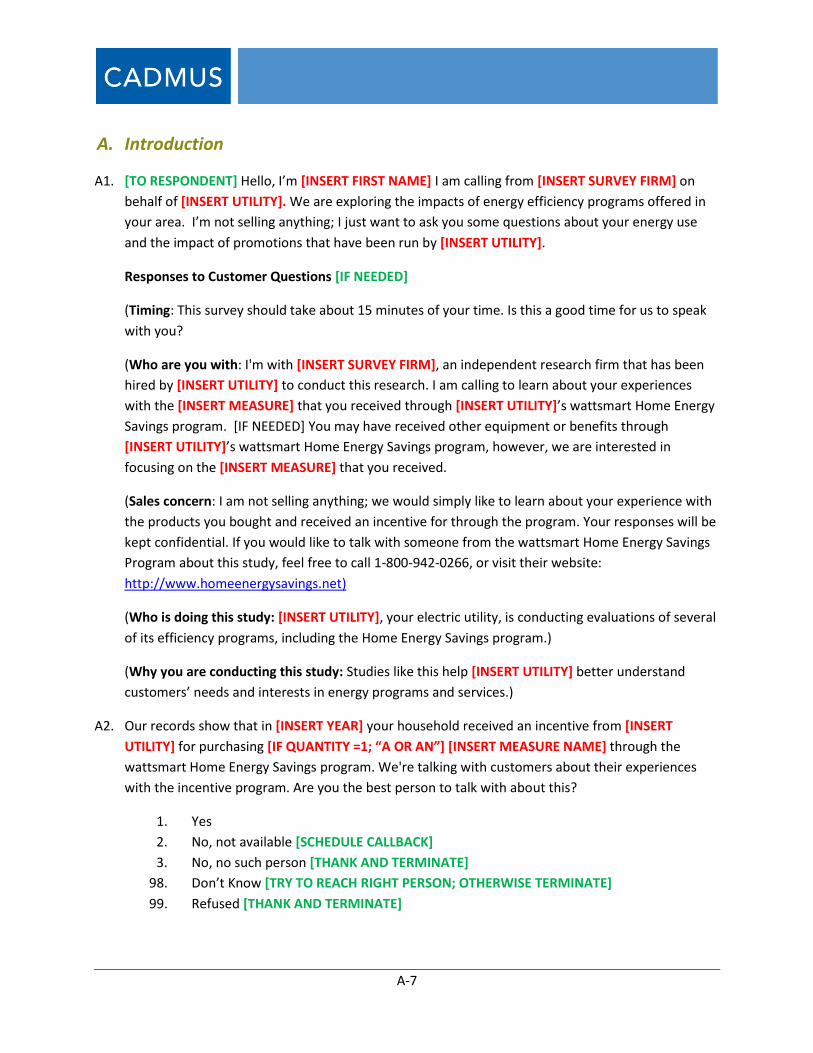
A-7
A. Introduction
A1. [TO RESPONDENT] Hello, I’m [INSERT FIRST NAME] I am calling from [INSERT SURVEY FIRM] on
behalf of [INSERT UTILITY]. We are exploring the impacts of energy efficiency programs offered in
your area. I’m not selling anything; I just want to ask you some questions about your energy use
and the impact of promotions that have been run by [INSERT UTILITY].
Responses to Customer Questions [IF NEEDED]
(Timing: This survey should take about 15 minutes of your time. Is this a good time for us to speak
with you?
(Who are you with: I'm with [INSERT SURVEY FIRM], an independent research firm that has been
hired by [INSERT UTILITY] to conduct this research. I am calling to learn about your experiences
with the [INSERT MEASURE] that you received through [INSERT UTILITY]’s wattsmart Home Energy
Savings program. [IF NEEDED] You may have received other equipment or benefits through
[INSERT UTILITY]’s wattsmart Home Energy Savings program, however, we are interested in
focusing on the [INSERT MEASURE] that you received.
(Sales concern: I am not selling anything; we would simply like to learn about your experience with
the products you bought and received an incentive for through the program. Your responses will be
kept confidential. If you would like to talk with someone from the wattsmart Home Energy Savings
Program about this study, feel free to call 1-800-942-0266, or visit their website:
http://www.homeenergysavings.net)
(Who is doing this study: [INSERT UTILITY], your electric utility, is conducting evaluations of several
of its efficiency programs, including the Home Energy Savings program.)
(Why you are conducting this study: Studies like this help [INSERT UTILITY] better understand
customers’ needs and interests in energy programs and services.)
A2. Our records show that in [INSERT YEAR] your household received an incentive from [INSERT
UTILITY] for purchasing [IF QUANTITY =1; “A OR AN”] [INSERT MEASURE NAME] through the
wattsmart Home Energy Savings program. We're talking with customers about their experiences
with the incentive program. Are you the best person to talk with about this?
1. Yes
2. No, not available [SCHEDULE CALLBACK]
3. No, no such person [THANK AND TERMINATE]
98. Don’t Know [TRY TO REACH RIGHT PERSON; OTHERWISE TERMINATE]
99. Refused [THANK AND TERMINATE]
A-8
A3. Were you the primary decision-maker when deciding to purchase the [INSERT MEASURE](S)]?
1. Yes
2. No [REQUEST TO SPEAK TO THE PRIMARY DECISION MAKER, IF AVAILABLE START
OVER, IF NOT, SCHEDULE TIME TO CALL BACK]
98. Don’t Know [THANK AND TERMINATE]
99. Refused [THANK AND TERMINATE]
A4. Have you, or anyone in your household, ever been employed by with [INSERT UTILITY] or any of its
affiliates?
1. Yes [THANK AND TERMINATE]
2. No [CONTINUE]
98. Don’t Know [THANK AND TERMINATE]
99. Refused [THANK AND TERMINATE]
B. Measure Verification
Now I have a few questions to verify my records are correct.
[FOR SECTION B “MEASURE VERIFICATION, FOLLOW THE RULES BELOW TO DETERMINE WHICH
QUESTIONS TO ASK BEFORE CONTINUING TO SECTION C:
IF MEASURE TYPE = SEALING OR SERVICE SKIP TO B7 AND ASK QUESTIONS B7 TO B8;
IF MEASURE TYPE = INSULATION OR WINDOWS SKIP TO B9 AND ASK QUESTIONS B9 TO B14;
ALL REMAINING MEASURE TYPES, CONTINUE TO B1 AND ASK QUESTIONS B1 TO B6]
B1. [INSERT UTILITY] records show that you applied for an incentive for [IF MEASURE QUANTITY = 1
SAY “A”] [IF MEASURE QUANTITY >1 INSERT MEASURE QUANTITY] [INSERT MEASURE](S) in [YEAR
OF PARTICIPATION]. Is that correct? [DO NOT READ RESPONSES]
[IF NEEDED SAY: “WE KNOW YOU MAY HAVE APPLIED FOR OTHER INCENTIVES, BUT FOR THIS
SURVEY, WE’D LIKE TO FOCUS ON JUST THIS ONE TYPE OF EQUIPMENT.”]
1. Yes [SKIP TO B4]
2. No, quantity is incorrect [CONTINUE TO B2]
3. No, measure is incorrect [SKIP TO B3]
4. No, both quantity and measure are incorrect [SKIP TO B3]
98. Don’t Know [SKIP TO B3]
99. Refused [TERMINATE]
A-9
B2. [ASK IF B1 = 2] For how many [INSERT MEASURE](S) did you apply for an incentive? [NUMERIC
OPEN ENDED. DOCUMENT AND USE AS QUANTITY FOR REMAINDER OF SURVEY]
1. [RECORD] [SKIP TO B4]
98. Don’t Know [SKIP TO B4]
99. Refused [SKIP TO B4]
B3. [ASK IF B1 = 3 OR 4 OR 98] Please tell me for what type of equipment you applied for an incentive?
[PROBE FOR MEASURE AND QUANTITY THEN SAY: “Thanks for your time, but unfortunately you
do not qualify for this survey.” THEN THANK AND TERMINATE]
1. [RECORD VERBATIM] [IF RESPONSE = SAME MEASURE, GO BACK TO B1]
98. Don’t Know [THANK AND TERMINATE]
99. Refused [THANK AND TERMINATE]
B4. Did [IF MEASURE QUANTITY >1 SAY “ALL OF”] the [INSERT MEASURE](S) get installed in your
home? [DO NOT READ RESPONSES]
1. Yes [SKIP TO C1]
2. No [CONTINUE TO B5]
98. Don’t know [SKIP TO C1]
99. Refused [SKIP TO C1]
[ASK B5 IF B4 = 2 AND MEASURE QUANTITY > 1 OTHERWISE SKIP TO B6]
B5. How many [INSERT MEASURE](S) were installed?
1. [RECORD # 1-100] [CONTINUE TO B6]
98. Don’t Know [CONTINUE TO B6]
99. Refused [CONTINUE TO B6]
A-10
B6. [ASK IF B4 = 2] Why haven't you installed the [INSERT MEASURE](S) [MULTIPLE RESPONSE UP TO
3; DO NOT READ, THEN SKIP TO C1]
1. Failed or broken unit [SKIP TO C1]
2. Removed because did not like it [SKIP TO C1]
3. Have not had time to install it yet [SKIP TO C1]
4. In-storage [SKIP TO C1]
5. Back up equipment to install when other equipment fails [SKIP TO C1]
6. Have not hired a contractor to install it yet [SKIP TO C1]
7. Purchased more than was needed [SKIP TO C1]
8. Other [RECORD] [SKIP TO C1]
98. Don’t Know [SKIP TO C1]
99. Refused [SKIP TO C1]
B7. [INSERT UTILITY] records show that you applied for an incentive for [INSERT MEASURE] in [YEAR
OF PARTICIPATION]. Is that correct? [DO NOT READ RESPONSES]
[IF NEEDED SAY: “WE KNOW YOU MAY HAVE APPLIED FOR OTHER INCENTIVES, BUT FOR THIS
SURVEY, WE’D LIKE TO FOCUS ON JUST THIS ONE TYPE OF EQUIPMENT.”]
1. Yes [SKIP TO C1]
2. No, measure is incorrect [SKIP TO B8]
98. Don’t Know [SKIP TO B8]
99. Refused [TERMINATE]
B8. [ASK IF B7 = 2 OR 98] Please tell me for what type of equipment you applied for an incentive?
[PROBE FOR MEASURE AND QUANTITY THEN SAY: “Thanks for your time, but unfortunately you
do not qualify for this survey.” THEN THANK AND TERMINATE]
1. [RECORD VERBATIM] [IF RESPONSE =SAME MEASURE, GO BACK TO B7]
98. Don’t Know [THANK AND TERMINATE]
99. Refused [THANK AND TERMINATE]
A-11
B9. [INSERT UTILITY] records show that you applied for an incentive for [INSERT MEASURE QUANTITY]
square feet of [INSERT MEASURE](S) in [YEAR OF PARTICIPATION]. Is that correct? [DO NOT READ
RESPONSES; IF CORRECTED YEAR IS NOT 2013 OR 2014, THANK AND TERMINATE,]
[IF NEEDED SAY: “WE KNOW YOU MAY HAVE APPLIED FOR OTHER INCENTIVES, BUT FOR THIS
SURVEY, WE’D LIKE TO FOCUS ON JUST THIS ONE TYPE OF EQUIPMENT.”]
1. Yes [SKIP TO B12]
2. No, quantity is incorrect [CONTINUE TO B10]
3. No, measure is incorrect [SKIP TO B11]
4. No, both quantity and measure are incorrect [SKIP TO B11]
98. Don’t Know [SKIP TO B11]
99. Refused [TERMINATE]
B10. [ASK IF B9 = 2] How many square feet of [INSERT MEASURE](S) did you apply for an incentive?
[NUMERIC OPEN ENDED. DOCUMENT AND USE AS QUANTITY FOR REMAINDER OF SURVEY]
1. [RECORD] [SKIP TO B12]
98. Don’t Know [SKIP TO B12]
99. Refused [SKIP TO B12]
B11. [ASK IF B9 = 3 OR 4 OR 98] Please tell me for what type of equipment you applied for an incentive?
[PROBE FOR MEASURE AND QUANTITY THEN SAY: “Thanks for your time, but unfortunately you
do not qualify for this survey.” THEN THANK AND TERMINATE]
1. [RECORD VERBATIM] [IF RESPONSE = SAME MEASURE, GO BACK TO B9]
98. Don’t Know [THANK AND TERMINATE]
99. Refused [THANK AND TERMINATE]
B12. Did all of the [INSERT MEASURE QUANTITY] square feet of [INSERT MEASURE](S) get installed in
your home? [DO NOT READ RESPONSES]
1. Yes [SKIP TO C1]
2. No [CONTINUE TO B13]
98. Don’t know [SKIP TO C1]
99. Refused [SKIP TO C1]
B13. What percentage of the [INSERT MEASURE](S) was installed?
1. [RECORD 0-100%] [CONTINUE TO B14]
98. Don’t Know [CONTINUE TO B14]
99. Refused [CONTINUE TO B14]
A-12
B14. Why haven’t you had a chance to install all [INSERT MEASURE QUANTITY] square feet of [INSERT
MEASURE] (S)? [MULTIPLE RESPONSE UP TO 3; DO NOT READ, THEN SKIP TO C1]
1. Failed or broken unit [SKIP TO C1]
2. Removed because did not like it [SKIP TO C1]
3. Have not had time to install it yet [SKIP TO C1]
4. In-storage [SKIP TO C1]
5. Back up equipment to install when other equipment fails [SKIP TO C1]
6. Have not hired a contractor to install it yet [SKIP TO C1]
7. Purchased more than was needed [SKIP TO C1]
8. Other [RECORD] [SKIP TO C1]
98. Don’t Know [SKIP TO C1]
99. Refused [SKIP TO C1]
A-13
C. Program Awareness & Purchase Decisions
C1. How did you first hear about [INSERT UTILITY]’s wattsmart Home Energy Savings program? [DO
NOT PROMPT. RECORD ONLY THE FIRST WAY HEARD ABOUT THE PROGRAM.]
1. Bill Inserts
2. Billboard/outdoor ad
3. Family/friends/word-of-mouth
4. Home Energy Reports
5. Home Shows/Trade Shows (Home and Garden Shows)
6. Internet Advertising/Online Ad
7. Newspaper/Magazine/Print Media
8. Northwest Energy Efficiency Alliance (NEEA)
9. Other website
10. Radio
11. Retailer/Store
12. Rocky Mountain Power/Pacific Power Representative
13. Rocky Mountain Power/Pacific Power website
14. Social Media
15. Sporting event
16. TV
17. wattsmart Home Energy Savings website
18. Other [RECORD VERBATIM]
98. [DO NOT READ] Don’t Know
99. [DO NOT READ] Refused
C2. [ASK IF C1 <> 13 0R 17, OTHERWISE SKIP TO C3] Have you been to the [INSERT UTILITY] wattsmart
Home Energy Savings program website? [DO NOT READ RESPONSES]
1. Yes
2. No
C3. [ASK IF C1 = 13 OR 17, OR IF C2 = 1, OTHERWISE SKIP TO C5] Was the website… [READ]
1. Very helpful [SKIP TO C5]
2. Somewhat helpful
3. Somewhat unhelpful
4. Very unhelpful
98. [DO NOT READ] Don’t Know
99. [DO NOT READ] Refused
A-14
C4. [ASK IF C3= 2, 3, OR 4. OTHERWISE SKIP TO C5] What would make the website more helpful for
you? [DO NOT READ RESPONSES, MARK ALL THAT APPLY]
1. Nothing, it is already very helpful for me.
2. Make the website easier to navigate or more user-friendly (clear hierarchy)
3. Make program information more clear and concise
4. Incorporate more visual information (charts, graphs, images) and less text
5. Provide easier access to customer service or FAQs
6. Other [RECORD]
C5. Please think back to the time when you were deciding to buy the energy saving [INSERT
MEASURE](S). What factors motivated you to purchase the [INSERT MEASURE](S)? [DO NOT READ.
INDICATE ALL THAT APPLY. ONCE THEY RESPONDENT HAS FINISHED, SAY: “ARE THERE ANY
OTHER FACTORS?”]
1. Old equipment didn’t work
2. Old equipment working poorly
3. The program incentive
4. A program affiliated contractor
5. Wanted to save energy
6. Wanted to reduce energy costs
7. Environmental concerns
8. Recommendation from other utility [PROBE: “WHAT UTILITY?” RECORD]
9. Recommendation of dealer/retailer [PROBE: “FROM WHICH STORE?” RECORD]
10. Recommendation from friend, family member, or colleague
11. Recommendation from a contractor
12. Advertisement in newspaper [PROBE: “FOR WHAT PROGRAM?” RECORD]
13. Radio advertisement [PROBE: “FOR WHAT PROGRAM?” RECORD]
14. Health or medical reasons
15. Maintain or increase comfort of home
16. Interested in new/updated technology
17. Other [RECORD]
98. Don’t Know
99. Refused

A-15
D. Measure Usage
[SAY “I HAVE SOME QUESTIONS ABOUT YOUR GENERAL HOUSEHOLD ENERGY USE AND
COMMON HOUSEHOLD APPLIANCES”]
D1. [IF MEASURE TYPE = CLOTHES WASHER, SKIP TO D2] Do you have a clothes washer installed in
your home?
1. Yes
2. No [SKIP TO D9]
98. Don’t Know [SKIP TO D9]
99. Refused [SKIP TO D9]
D2. Approximately how many loads of clothes does your household wash in a typical week?
1. [RECORD]
98. Don’t Know
99. Refused
D3. [ASK IF MEASURE TYPE = CLOTHES WASHER, OTHERWISE SKIP TO D5] How does the number of
wash loads you do now compare to the number that you did with your old clothes washer? [DO
NOT READ RESPONSES]
1. Same [SKIP TO D5]
2. Different [CONTINUE TO D4]
98. Don’t Know [SKIP TO D5]
99. Refused [SKIP TO D5]
D4. [ASK IF D3 = 2]Do you do more or fewer loads now than you did before? Could you estimate a
percentage?
1. More loads now, Record percentage [MUST BE GREATER THAN 100%, EG 125% FOR
25% MORE]
2. Fewer loads now, Record percentage [MUST BE LESS THAN 100%, EG 75% FOR 25%
LESS THAN BEFORE]
98. Don’t Know
99. Refused

A-16
D5. On what percentage of loads do you use a high-speed spin cycle? [IF NEEDED: HIGH-SPEED SPIN
CYCLES REMOVE MORE WATER FROM THE LOAD, RESULTING IN SHORTER DRYING TIMES]
1. Never
2. LESS THAN 25%
3. 25-50%
4. 50-75%
5. 75-99%
6. Always or 100% [SKIP TO D7]
98. [DO NOT READ] Don’t know [SKIP TO D7]
99. [DO NOT READ] Refused [SKIP TO D7]
D6. [ASK IF D5 = 1-5] When you do not use the high spin cycle, what is your reason? [DO NOT READ.
INDICATE ALL THAT APPLY]
1. Noise/vibration
2. Impact on clothing
3. Always use high spin
4. Other [RECORD]
98. [DO NOT READ]Don’t know
99. [DO NOT READ] Refused
D7. What percentage of your loads do you dry using a clothes dryer? [READ CATEGORIES IF NEEDED]
1. Never [SKIP TO D9]
2. LESS THAN 25%
3. 25-50%
4. 50-75%
5. 75- 99%
6. Always or 100%
98. Don’t know [SKIP TO D9]
99. Refused [SKIP TO D9]
D8. When you dry your clothes do you… [READ]
1. Use a timer to determine drying times.
2. Use the dryer’s moisture sensor to determine when the load is dry.
3. Other [SPECIFY]
98. [DO NOT READ] Don’t know
99. [DO NOT READ] Refused
A-17
D9. How many times a week do you use a dishwasher?
1. [RECORD]
2. Don’t have a dishwasher
98. Don’t Know
99. Refused
[IF MEASURE TYPE= HEATING SKIP TO D13 OR HEATING/COOLING SKIP TO D20]
D10. What type of heating system do you primarily use… [READ]
1. Furnace
2. Boiler
3. Air Source Heat Pump
4. Ground Source Heat Pump
5. Ductless Heat Pump
6. Stove
7. Baseboard
8. No heating system [SKIP TO D13]
9. Other [SPECIFY]
98. [DO NOT READ] Don’t Know
99. [DO NOT READ] Refused
D11. How many years old is the heating system?
1. [RECORD]
98. Don’t Know
99. Refused
D12. What type of fuel does the heating system use… [READ]
1. Gas
2. Electric
3. Oil
4. Propane
5. Coal
6. Wood
7. Other [SPECIFY]
98. [DO NOT READ] Don’t Know
99. [DO NOT READ] Refused

A-18
D13. [IF MEASURE TYPE= COOLING SKIP TO D23] What type of cooling system do you primarily use [IF
MEASURE TYPE = ROOM AC THEN SAY “BESIDES THE ROOM AIR CONDITIONER”]? A… [READ,
MULTIPLE CHOICES ALLOWED]
1. Central Air Conditioner
2. Evaporative Cooler
3. Air Source Heat Pump
4. Ground Source Heat Pump
5. Ductless heat pump
6. Whole house fan
7. No central cooling system [SKIP TO D15]
8. Other [SPECIFY]
98. [DO NOT READ] Don’t Know
99. [DO NOT READ] Refused
D14. How many years old is your current cooling system?
1. [RECORD]
98. Don’t Know
99. Refused
D15. [ASK IF MEASURE TYPE = LIGHTING] in which room(S) [is/are] the lighting fixture(s) installed?
[MULTIPLE RESPONSES ALLOWED]
1. Living/family room
2. Bedroom
3. Unoccupied bedroom
4. Bathroom
5. Kitchen
6. Garage
7. Office
8. Attic
9. Closet/storage
10. Hallway
11. Exterior
98. Don’t Know
99. Refused
[FOR QUESTIONS D16 - D24 USE THE FOLLOWING SKIP PATTERN
FOR MEASURE TYPES OTHER, CLOTHES WASHER, ROOM AC, AND LIGHTING: READ QUESTIONS D16 TO
D17 THEN SKIP TO E1;
FOR MEASURE TYPE WINDOWS: READ QUESTIONS D18 AND D19 THEN SKIP TO E1;
A-19
FOR MEASURE TYPE HEATING: READ QUESTIONS D20 TO D22 THEN SKIP TO E1
FOR MEASURE TYPE COOLING: READ QUESTIONS D23 TO D24 THEN SKIP TO E1;
FOR MEASURE TYPE HEATING/COOLING: READ QUESTIONS D20 TO D24 THEN SKIP TO E1;
FOR MEASURE TYPES SEALING, INSULATION AND SERVICE: SKIP TO E1]
D16. Was the purchase of your new [INSERT MEASURE](S) intended to replace [AN] old [INSERT
MEASURE TYPE]?
1. Yes [CONTINUE TO D17]
2. No [SKIP TO E1]
98. Don’t Know [SKIP TO E1]
99. Refused [SKIP TO E1]
D17. [ASK IF D16 = 1] What did you do with the old [INSERT MEASURE TYPE] after you got your new
[INSERT MEASURE](S)? [READ CATEGORIES IF NEEDED]
1. Sold or given away [SKIP TO E1]
2. Recycled [SKIP TO E1]
3. Installed in another location in the home [SKIP TO E1]
4. Still in home but permanently removed [stored in garage, etc.] [SKIP TO E1]
5. Thrown away [SKIP TO E1]
98. [DO NOT READ] Don’t Know [SKIP TO E1]
99. [DO NOT READ] Refused [SKIP TO E1]
D18. [ASK IF MEASURE TYPE= WINDOWS AND (B9 = 1 OR B13.1>0%). OTHERWISE SKIP TO E1] What
type of windows did you have before the new windows were installed?
1. Single pane [OLDER WINDOWS]
2. Double Pane [NEWER WINDOWS]
3. Triple Pane [RARE]
98. Don’t Know
99. Refused
D19. [ASK IF MEASURE = WINDOWS AND (B9= 1 OR B13.1>0%), OTHERWISE SKIP TO E1] What type of
window frames (not window trim, which is almost always wood) did you have before the new
windows were installed?
1. Wood
2. Vinyl
3. Metal
98. Don’t Know
99. Refused
A-20
[ASK D20 TO D22 IF MEASURE TYPE = HEATING OR HEATING/COOLING. OTHERWISE SKIP TO E1]
D20. What type of heating system did you have before the new [INSERT MEASURE] was installed?
1. Furnace
2. Boiler
3. Air Source Heat Pump
4. Ground Source Heat Pump
5. Ductless Heat Pump
6. Stove
7. Baseboard
8. No heating system before [SKIP TO E1]
9. Other [SPECIFY]
98. [DO NOT READ] Don’t Know
99. [DO NOT READ] Refused
D21. How many years old was the previous heating system?
1. [RECORD]
98. Don’t Know
99. Refused
D22. What type of fuel does the new heating system use… [READ]
1. Gas
2. Electric
3. Oil
4. Propane
5. Coal
6. Wood
7. Other [SPECIFY]
98. [DO NOT READ] Don’t Know
99. [do not read] Refused
A-21
[ASK D23 TO D24 IF MEASURE TYPE = COOLING OR HEATING/COOLING]
D23. What type of cooling system did you have before the new [INSERT MEASURE] was installed?
[READ]
1. Central Air Conditioner
2. Room Air Conditioner
3. Evaporative Cooler
4. Air Source Heat Pump
5. Ground Source Heat Pump
6. Ductless Heat Pump
7. Whole house fan
8. No cooling system before [SKIP TO E1]
9. Other [SPECIFY]
98. [DO NOT READ] Don’t Know
99. [DO NOT READ] Refused
D24. How many years old was the previous cooling system?
1. [RECORD]
98. Don’t Know
99. Refused
E. Satisfaction
E1. Overall, how satisfied are you with your [INSERT MEASURE](S) Would you say you are…? [READ
CATEGORIES; RECORD FIRST RESPONSE ONLY]
1. Very Satisfied
2. Somewhat Satisfied
3. Not Very Satisfied
4. Not At All Satisfied
98. [DO NOT READ] Don’t Know
99. [DO NOT READ] Refused
E2. Did a contractor install the [INSERT MEASURE](S) for you?
1. Yes
2. No
98. Don’t Know
99. Refused

A-22
E3. [ASK IF E2=1] How satisfied were you with the contractor that installed the [INSERT MEASURE](S)
for you? [READ CATEGORIES; RECORD FIRST RESPONSE ONLY]
1. Very Satisfied
2. Somewhat Satisfied
3. Not Very Satisfied
4. Not At All Satisfied
98. [DO NOT READ] Don’t Know
99. [DO NOT READ] Refused
E4. [IF E3 = 3 OR 4] Why were you not satisfied with the contractor that installed the [INSERT
MEASURE](S)?
1. [RECORD]
98. Don’t know
99. Refused
E5. How easy did you find filling out the wattsmart Home Energy Savings Program incentive
application? [READ CATEGORIES; RECORD FIRST RESPONSE ONLY]
1. Very Easy
2. Somewhat Easy
3. Not Very Easy [PROBE FOR REASON AND RECORD]
4. Not At All Easy [PROBE FOR REASON AND RECORD]
98. [DO NOT READ] Don’t Know
99. [DO NOT READ] Refused
E6. How satisfied were you with the amount of the incentive you received for the [INSERT
MEASURE](S)?
1. Very Satisfied
2. Somewhat Satisfied
3. Not Very Satisfied [PROBE FOR REASON AND RECORD]
4. Not At All Satisfied [PROBE FOR REASON AND RECORD]
98. Don’t Know
99. Refused

A-23
E7. After you submitted the incentive application for the [INSERT MEASURE](S), how long did it take to
receive the incentive check from [INSERT UTILITY]? Was it… [READ CATEGORIES IF NEEDED,
RECORD ONLY FIRST RESPONSE]
1. Less than 4 weeks
2. Between 4 and 6 weeks
3. Between 7 and 8 weeks
4. More than 8 weeks
5. Have not received the incentive yet
98. [DO NOT READ] Don’t Know [SKIP TO E9]
99. [DO NOT READ] Refused [SKIP TO E9]
E8. [ASK IF E7<> 5] Were you satisfied with how long it took to receive the incentive?
1. Yes
2. No [PROBE FOR REASON AND RECORD]
98. Don’t Know
99. Refused
E9. How satisfied were you with the entire application process?
1. Very Satisfied
2. Somewhat Satisfied
3. Not Very Satisfied [PROBE FOR REASON AND RECORD]
4. Not At All Satisfied [PROBE FOR REASON AND RECORD]
E10. Overall, how satisfied are you with the wattsmart Home Energy Savings program? [READ
CATEGORIES; RECORD ONLY FIRST RESPONSE]
1. Very Satisfied [PROBE FOR REASON AND RECORD]
2. Somewhat Satisfied [PROBE FOR REASON AND RECORD]
3. Not Very Satisfied [PROBE FOR REASON AND RECORD]
4. Not At All Satisfied [PROBE FOR REASON AND RECORD]
98. [DO NOT READ] Don’t Know
99. [DO NOT READ] Refused
A-24
E11. Did your participation in [INSERT UTILITY]’s wattsmart Home Energy Savings Program cause your
satisfaction with [INSERT UTILITY] to…
1. Increase
2. Stay the same
3. Decrease
98. [DO NOT READ] Don’t Know
99. [DO NOT READ] Refused
F. Freeridership
Now I’d like to talk with you a little more about the [INSERT MEASURE](S) you purchased.
F1. When you first heard about the incentive from [INSERT UTILITY], had you already been planning to
purchase the [INSERT MEASURE](S)?
1. Yes
2. No [SKIP TO F4]
98. Don’t Know [SKIP TO F4]
99. Refused [SKIP TO F4]
F2. Ok. Had you already purchased or installed the new [INSERT MEASURE](S) before you learned
about the incentive from the wattsmart Program?
1. Yes
2. No [SKIP TO F4]
98. Don’t Know [SKIP TO F4]
99. Refused [SKIP TO F4]
F3. Just to confirm, you learned about the [INSERT UTILITY] rebate program after you had already
purchased or installed the [INSERT MEASURE](S) ?
1. Yes [SKIP TO F13]
2. No
98. Don’t Know
99. Refused
[IF F3= 1 SKIP TO F13]

A-25
F4. Would you have purchased the same [INSERT MEASURE](S) without the incentive from the
wattsmart Home Energy Savings program?
1. Yes [SKIP TO F6]
2. No
98. Don’t Know
99. Refused
[IF F4 = 1 THEN SKIP TO F6]
F5. [ASK IF F4 = 2, -98 OR -99] Help me understand, would you have purchased something without the
wattsmart Home Energy Savings program incentive? [DO NOT READ RESPONSES]
1. Yes, I would have purchased something
2. No, I would not have purchased anything [SKIP TO F9]
98. Don’t Know [SKIP TO F13]
99. Refused [SKIP TO F13]
[IF F5 = 2 SKIP TO F9. IF F5 = -98 OR -99 SKIP TO F13]
F6. [ASK IF F4= 1 OR F5 = 1] Let me make sure I understand. When you say you would have purchased
[A] [MEASURE](S) without the program incentive, would you have purchased [A] [INSERT
MEASURE](S)] THAT [WAS/WERE] JUST AS ENERGY EFFICIENT”?
1. Yes
2. No
98. Don’t Know
99. Refused
F7. [ASK IF F4= 1 OR F5 = 1 AND MEASURE QUANTITY >1] Without the program incentive would you
have purchased the same amount of [INSERT MEASURE](S)?
1. Yes, I would have purchased the same amount
2. No, I would have purchased less
98. Don’t Know
99. Refused
A-26
F8. [ASK IF F4= 1 OR F5 = 1] Without the program incentive would you have purchased the [INSERT
MEASURE](S)… [READ]
1. At the same time
2. Within one year?
3. In more than one year?
98. [DO NOT READ] Don’t Know
99. [DO NOT READ] Refused
[SKIP TO F13]
F9. [ASK IF F5=2] To confirm, when you say you would not have purchased the same [INSERT
MEASURE](S) without the program incentive, do you mean you would not have purchased the
[INSERT MEASURE](S) at all?
1. Yes
2. No
98. Don’t Know
99. Refused
[IF F9 = 1 SKIP TO F13]
F10. [ASK IF F9 = 2, -98, -99] Again, help me understand. Without the program incentive, would you
have purchased the same type of [INSERT MEASURE](S) but [A] [[INSERT MEASURE](S)] THAT
[WAS/WERE] NOT AS ENERGY EFFICIENT?
1. Yes
2. No
98. Don’t Know
99. Refused
F11. [ASK IF F9= 2, -98, -99 AND QTY MEASURE>1] Without the program incentive would you have
purchased the same amount of [INSERT MEASURE](S)?
1. Yes, I would purchase the same amount
2. No, I would have purchased less
98. Don’t Know
99. Refused
A-27
F12. [ASK IF F9 = 2, -98, -99]And, would you have purchased the [INSERT MEASURE](S)… [READ]
1. At the same time
2. Within one years?
3. In more than one year?
98. [DO NOT READ] Don’t Know
99. [DO NOT READ] Refused
F13. In your own words, please tell me the influence the Home Energy Saving incentive had on your
decision to purchase [INSERT MEASURE](S)?
1. ______ [RECORD RESPONSE]
G. Spillover
G1. Since participating in the program, have you added any other energy efficient equipment or
services in your home that were not incentivized through the wattsmart Home Energy Savings
Program?
1. Yes
2. No
98. Don’t Know
99. Refused
[IF G1 = 2, -98 OR -99 SKIP TO H1]
A-28
G2. What high-efficiency energy-saving equipment or services have you purchased since applying for
the incentive, not including the [INSERT MEASURE] that we have been discussing today? [LIST OF
OTHER ELIGIBLE APPLIANCES AND MEASURES OTHER THAN THOSE LISTED IN PROGRAM
RECORDS. PROMPT IF NEEDED]
1. Clothes Washer [RECORD QUANTITY]
2. Refrigerator [RECORD QUANTITY]
3. Dishwasher [RECORD QUANTITY]
4. Windows [RECORD QUANTITY IN SQ FT]
5. Fixtures [RECORD QUANTITY]
6. Heat Pump [RECORD QUANTITY]
7. Central Air Conditioner [RECORD QUANTITY]
8. Room Air Conditioner [RECORD QUANTITY]
9. Ceiling Fans [RECORD QUANTITY]
10. Electric Storage Water Heater [RECORD QUANTITY]
11. Electric Heat Pump Water Heater [RECORD QUANTITY]
12. CFLs [RECORD QUANTITY]
13. LEDs [RECORD QUANTITY]
14. Insulation [RECORD QUANTITY IN SQ FT]
15. Air Sealing [RECORD QUANTITY IN CFM REDUCTION]
16. Duct Sealing [RECORD QUANTITY IN CFM REDUCTION]
17. Programmable thermostat [RECORD QUANTITY]
18. Other [RECORD] [RECORD QUANTITY]
19. None
98. Don’t Know
99. Refused
[IF G2 = 12 (ONLY), -98 OR -99 SKIP TO H1. REPEAT G3 THROUGH G5 FOR ALL RESPONSES TO G2]
G3. In what year did you purchase [INSERT MEASURE TYPE FROM G2]?
1. 2013
2. 2014
3. Other [RECORD YEAR]
98. Don’t Know
99. Refused
A-29
G4. Did you receive an incentive for [INSERT MEASURE TYPE FROM G2]?
1. Yes [PROBE AND RECORD]
2. No
98. Don’t Know
99. Refused
G5. How influential would you say the wattsmart Home Energy Savings program was in your decision to
add the [INSERT MEASURE FROM G2] to your home? Was it… [REPEAT FOR EACH MEASURE
LISTED IN G2]
1. Highly Influential
2. Somewhat Influential
3. Not very influential
4. Not at all influential
98. Don’t Know
99. Refused
H. Demographics
I have just a few more questions about your household. Again, all your answers will be strictly
confidential.
H1. Which of the following best describes your house? [READ LIST]:
1. Single-family home
2. Townhouse or duplex
3. Mobile home or trailer
4. Apartment building with 4 or more units
5. Other [RECORD]
98. [DO NOT READ] Don’t Know
99. [DO NOT READ] refused
H2. Do you rent or own your home?
1. Own
2. Rent
3. Other [RECORD]
98. Don’t Know
99. Refused
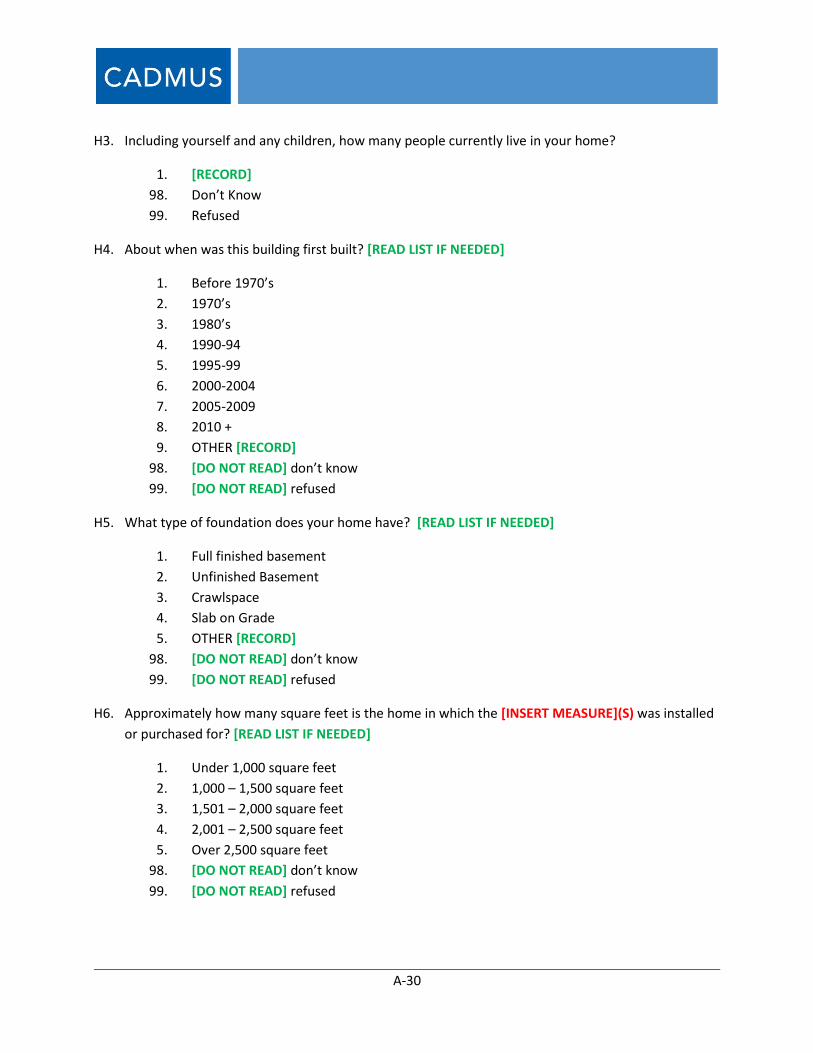
A-30
H3. Including yourself and any children, how many people currently live in your home?
1. [RECORD]
98. Don’t Know
99. Refused
H4. About when was this building first built? [READ LIST IF NEEDED]
1. Before 1970’s
2. 1970’s
3. 1980’s
4. 1990-94
5. 1995-99
6. 2000-2004
7. 2005-2009
8. 2010 +
9. OTHER [RECORD]
98. [DO NOT READ] don’t know
99. [DO NOT READ] refused
H5. What type of foundation does your home have? [READ LIST IF NEEDED]
1. Full finished basement
2. Unfinished Basement
3. Crawlspace
4. Slab on Grade
5. OTHER [RECORD]
98. [DO NOT READ] don’t know
99. [DO NOT READ] refused
H6. Approximately how many square feet is the home in which the [INSERT MEASURE](S) was installed
or purchased for? [READ LIST IF NEEDED]
1. Under 1,000 square feet
2. 1,000 – 1,500 square feet
3. 1,501 – 2,000 square feet
4. 2,001 – 2,500 square feet
5. Over 2,500 square feet
98. [DO NOT READ] don’t know
99. [DO NOT READ] refused
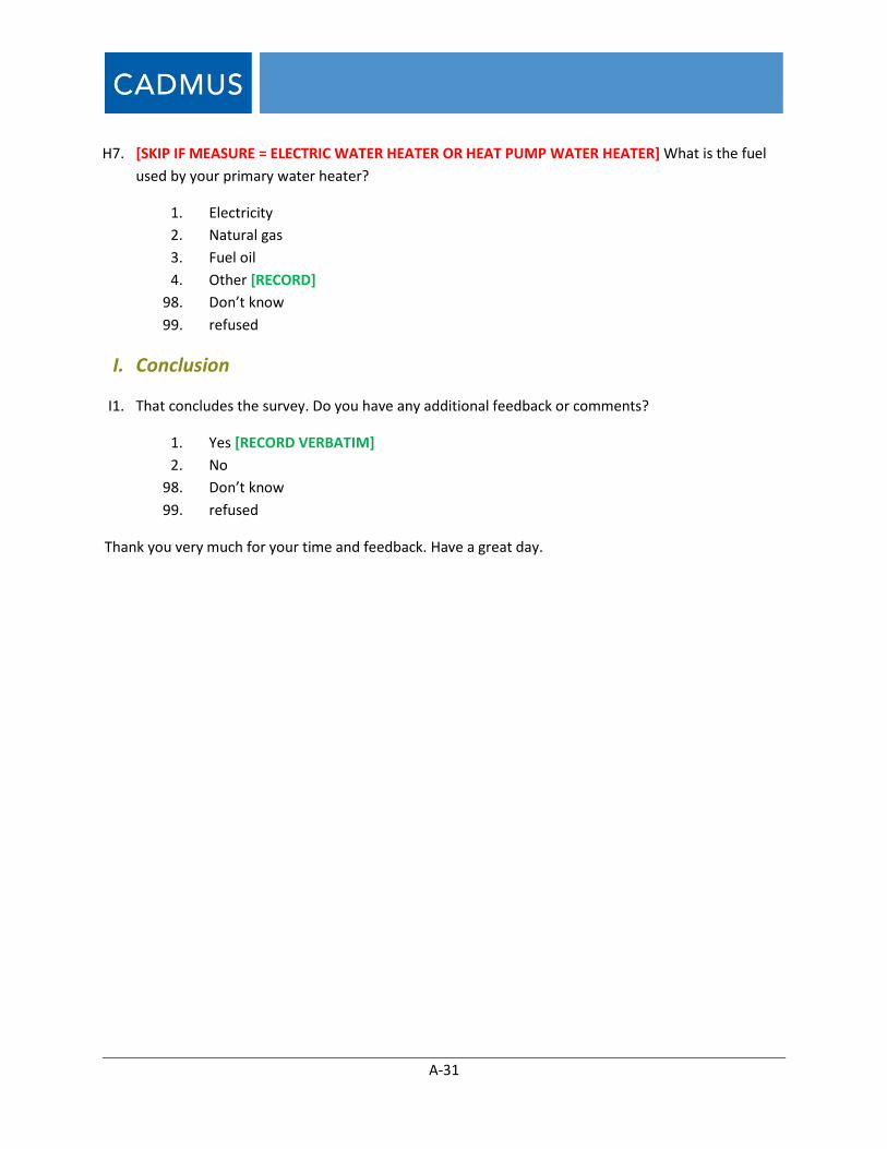
A-31
H7. [SKIP IF MEASURE = ELECTRIC WATER HEATER OR HEAT PUMP WATER HEATER] What is the fuel
used by your primary water heater?
1. Electricity
2. Natural gas
3. Fuel oil
4. Other [RECORD]
98. Don’t know
99. refused
I. Conclusion
I1. That concludes the survey. Do you have any additional feedback or comments?
1. Yes [RECORD VERBATIM]
2. No
98. Don’t know
99. refused
Thank you very much for your time and feedback. Have a great day.
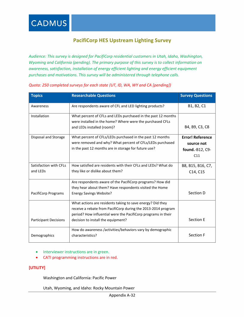
Appendix A-32
PacifiCorp HES Upstream Lighting Survey
Audience: This survey is designed for PacifiCorp residential customers in Utah, Idaho, Washington,
Wyoming and California (pending). The primary purpose of this survey is to collect information on
awareness, satisfaction, installation of energy efficient lighting and energy efficient equipment
purchases and motivations. This survey will be administered through telephone calls.
Quota: 250 completed surveys for each state (UT, ID, WA, WY and CA [pending])
Topics Researchable Questions Survey Questions
Awareness Are respondents aware of CFL and LED lighting products? B1, B2, C1
Installation What percent of CFLs and LEDs purchased in the past 12 months
were installed in the home? Where were the purchased CFLs
and LEDs installed (room)? B4, B9, C3, C8
Disposal and Storage What percent of CFLs/LEDs purchased in the past 12 months
were removed and why? What percent of CFLs/LEDs purchased
in the past 12 months are in storage for future use?
Error! Reference
source not
found.-B12, C9-
C11
Satisfaction with CFLs
and LEDs
How satisfied are residents with their CFLs and LEDs? What do
they like or dislike about them?
B8, B15, B16, C7,
C14, C15
PacifiCorp Programs
Are respondents aware of the PacifiCorp programs? How did
they hear about them? Have respondents visited the Home
Energy Savings Website? Section D
Participant Decisions
What actions are residents taking to save energy? Did they
receive a rebate from PacifiCorp during the 2013-2014 program
period? How influential were the PacifiCorp programs in their
decision to install the equipment? Section E
Demographics
How do awareness /activities/behaviors vary by demographic
characteristics? Section F
Interviewer instructions are in green.
CATI programming instructions are in red.
[UTILITY]
Washington and California: Pacific Power
Utah, Wyoming, and Idaho: Rocky Mountain Power

Appendix A-33
A. Introduction
A1. [TO RESPONDENT] Hello, I’m [INSERT FIRST NAME], calling from [INSERT SURVEY FIRM], on behalf
of [UTILITY]. May I please speak with [INSERT NAME]?
Hello, we are conducting a survey about household lighting and home energy use and would like to
ask you some questions about your household’s lighting and energy use. We would greatly
appreciate your opinions.
[IF NOT AVAILABLE, ASK FOR AN ADULT IN THE HOUSEHOLD WHO IS RESPONSIBLE FOR
PURCHASING THE LIGHT BULBS. IF NO ONE APPROPRIATE IS AVAILABLE, TRY TO RESCHEDULE
AND THEN TERMINATE. IF TRANSFERRED TO ANOTHER PERSON, REPEAT INTRO AND THEN
CONTINUE.]
Responses to Customer Questions [IF NEEDED]
(Timing: This survey should take about 10 to 15 minutes of your time. Is this a good time for us to
speak with you?)
(Who are you with: I'm with [INSERT SURVEY FIRM], an independent research firm that has been
hired by [UTILITY] to conduct this research. I am calling to learn about your household lighting and
home energy use)
(Sales concern: I am not selling anything; we would simply like to learn about your household
lighting and home energy use. Your responses will be kept confidential. If you would like to talk
with someone from the Home Energy Savings Program about this study, feel free to call 1-800-942-
0266, or visit their website: http://www.homeenergysavings.net/.)
(Who is doing this study: [INSERT UTILITY], your electric utility, is conducting evaluations of
several of its efficiency programs.)
(Why are you conducting this study: Studies like this help [INSERT UTILITY] better understand
customers’ need and interest in energy programs and services.)
A2. This call may be monitored for quality assurance. First, are you the person who usually purchases
light bulbs for your household?
1. Yes
2. No, but person who does can come to phone [START OVER AT INTRO SCREEN WITH
NEW RESPONDENT]
3. No, and the person who does is not available [SCHEDULE CALLBACK]
98. Don’t Know [THANK AND TERMINATE]
99. Refused [THANK AND TERMINATE]

Appendix A-34
A3. Have you, or anyone in your household, ever been employed by or affiliated with [INSERT UTILITY]
or any of its affiliates?
1. Yes [THANK AND TERMINATE]
2. No [CONTINUE]
98. Don’t Know [CONTINUE]
99. Refused [THANK AND TERMINATE]
B. CFL Awareness and Purchases
B1. Before this call today, had you ever heard of a type of energy-efficient light bulb called a “compact
fluorescent light bulb”, or CFL, for short?
1. Yes [SKIP TO B3]
2. No
B2. CFLs usually do not look like traditional incandescent light bulbs. The most common type of CFL has
a spiral shape, resembling soft-serve ice cream, and it fits in a regular light bulb socket. Before
today, had you heard of CFLs?
1. Yes
2. No [SKIP TO C1]
B3. I have some questions about your lighting purchases during the last twelve months. Did you
purchase any CFLs in the last twelve months?
1. Yes
2. No [SKIP TO C1]
98. Don’t Know [SKIP TO C1]
99. Refused [SKIP TO C1]
B4. During the last twelve months, how many CFLs did you or your household purchase? Please try to
estimate the total number of individual CFL bulbs, as opposed to packages. [IF “DON’T KNOW,”
PROBE: “IS IT LESS THAN OR MORE THAN FIVE BULBS?” WORK FROM THERE TO GET AN
ESTIMATE]
1. [RECORD # OF CFLS: NUMERIC OPEN END] [IF QUANTITY=0, SKIP TO C1]
98. Don’t Know [PROBE: “IS IT LESS THAN OR MORE THAN FIVE BULBS?” WORK FROM
THERE TO GET AN ESTIMATE] [IF UNABLE TO GET AN ANSWER,
SKIP TO C1]
99. Refused [SKIP TO C1]

Appendix A-35
B5. Where did you purchased the [B4.1] CFLs? [PROBE FOR RETAIL CHAINS OR ONLINE] [DO NOT
READ, MULTIPLE REPSONSES ALLOWED]
1. Ace Hardware [CITY, STATE, # PURCHASED]
2. Broulim’s Fresh Foods [CITY, STATE, # PURCHASED]
3. Barrett’s Foodtown [CITY, STATE, # PURCHASED]
4. Batteries Plus [CITY, STATE, # PURCHASED]
5. Bi-Mart [CITY, STATE, # PURCHASED]
6. Big Lots [CITY, STATE, # PURCHASED]
7. Corner Grocery & Hardware [CITY, STATE, # PURCHASED]
8. Costco [CITY, STATE, # PURCHASED]
9. Delta Jubilee Foods [CITY, STATE, # PURCHASED]
10. Do It Best [CITY, STATE, # PURCHASED]
11. Dollar Tree [CITY, STATE, # PURCHASED]
12. Family Dollar [CITY, STATE, # PURCHASED]
13. Fresh Markets [CITY, STATE, # PURCHASED]
14. Kamas Foodtown [CITY, STATE, # PURCHASED]
15. Kroger – Fred Meyer [CITY, STATE, # PURCHASED]
16. Griffith Foodtown [CITY, STATE, # PURCHASED]
17. Gunnison Market [CITY, STATE, # PURCHASED]
18. Hess Lumber Co [CITY, STATE, # PURCHASED]
19. Habitat for Humanity [CITY, STATE, # PURCHASED]
20. Harmons [CITY, STATE, # PURCHASED]
21. Lowe’s [CITY, STATE, # PURCHASED]
22. Menards [CITY, STATE, # PURCHASED]
23. Petersons Fresh Market [CITY, STATE, # PURCHASED]
24. Rancho Markets [CITY, STATE, # PURCHASED]
25. Ream’s Foods [CITY, STATE, # PURCHASED]
26. Ridley’s [CITY, STATE, # PURCHASED]
27. Safeway [CITY, STATE, # PURCHASED]
28. Sam’s Club [CITY, STATE, # PURCHASED]
29. Smith’s [CITY, STATE, # PURCHASED]
30. Stokes Market Place [CITY, STATE, # PURCHASED]
31. Sutherlands [CITY, STATE, # PURCHASED]
32. Thomas Market [CITY, STATE, # PURCHASED]
33. Target [CITY, STATE, # PURCHASED]
34. Home Depot [CITY, STATE, # PURCHASED]
35. The Market [CITY, STATE, # PURCHASED]
36. True Value Hardware [CITY, STATE, # PURCHASED]
37. Walgreens [CITY, STATE, # PURCHASED]
38. Walmart [CITY, STATE, # PURCHASED]
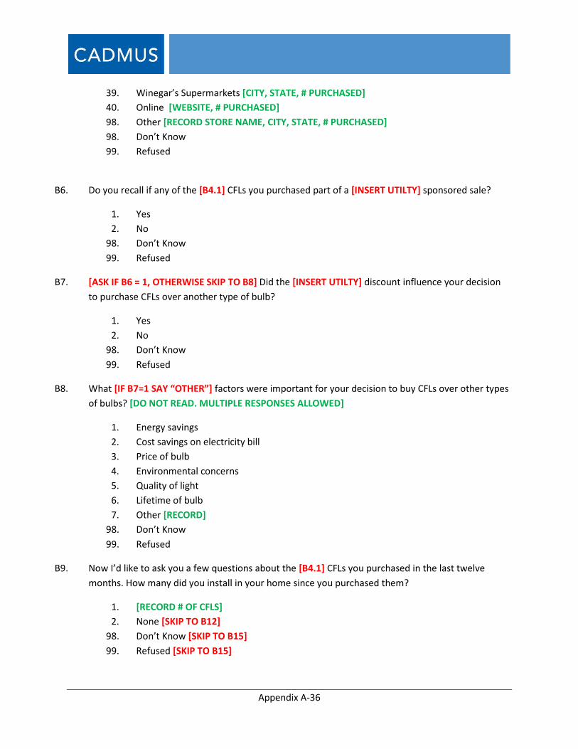
Appendix A-36
39. Winegar’s Supermarkets [CITY, STATE, # PURCHASED]
40. Online [WEBSITE, # PURCHASED]
98. Other [RECORD STORE NAME, CITY, STATE, # PURCHASED]
98. Don’t Know
99. Refused
B6. Do you recall if any of the [B4.1] CFLs you purchased part of a [INSERT UTILTY] sponsored sale?
1. Yes
2. No
98. Don’t Know
99. Refused
B7. [ASK IF B6 = 1, OTHERWISE SKIP TO B8] Did the [INSERT UTILTY] discount influence your decision
to purchase CFLs over another type of bulb?
1. Yes
2. No
98. Don’t Know
99. Refused
B8. What [IF B7=1 SAY “OTHER”] factors were important for your decision to buy CFLs over other types
of bulbs? [DO NOT READ. MULTIPLE RESPONSES ALLOWED]
1. Energy savings
2. Cost savings on electricity bill
3. Price of bulb
4. Environmental concerns
5. Quality of light
6. Lifetime of bulb
7. Other [RECORD]
98. Don’t Know
99. Refused
B9. Now I’d like to ask you a few questions about the [B4.1] CFLs you purchased in the last twelve
months. How many did you install in your home since you purchased them?
1. [RECORD # OF CFLS]
2. None [SKIP TO B12]
98. Don’t Know [SKIP TO B15]
99. Refused [SKIP TO B15]
Appendix A-37
B10. Have you since removed any of those CFL bulbs from the sockets?
1. Yes [ASK “HOW MANY DID YOU REMOVE?” RECORD # OF CFLS]
2. No [SKIP TO B12]
98. Don’t Know
99. Refused
B11. What were the reasons you removed the [B10.1] purchased CFLs from the sockets? [QUANTITIES
SHOULD ADD TO B10.1, IF NOT, ASK “WHAT ABOUT THE REMAINING BULBS YOU REMOVED?]
[DO NOT READ, MULTIPLE RESPONSES ALLOWED]
1. Bulb burned out [ASK: “HOW MANY DID YOU REMOVE BECAUSE OF THIS?” RECORD #
OF CFLS]
2. Bulbs were too bright [ASK: “HOW MANY DID YOU REMOVE BECAUSE OF THIS?”
RECORD # OF CFLS]
3. Bulbs were not bright enough [ASK: “HOW MANY DID YOU REMOVE BECAUSE OF
THIS?” RECORD # OF CFLS]
4. Delay in light coming on [ASK: “HOW MANY DID YOU REMOVE BECAUSE OF THIS?”
RECORD # OF CFLS]
5. Did not work with dimmer/3-way switch [ASK: “HOW MANY DID YOU REMOVE
BECAUSE OF THIS?” RECORD # OF CFLS]
6. Didn’t fit properly [ASK: “HOW MANY DID YOU REMOVE BECAUSE OF THIS?” RECORD #
OF CFLS]
7. Stuck out of fixture [ASK: “HOW MANY DID YOU REMOVE BECAUSE OF THIS?” RECORD
# OF CFLS]
8. Light color [ASK: “HOW MANY DID YOU REMOVE BECAUSE OF THIS?” RECORD # OF
CFLS]
9. Concerned about mercury [ASK: “HOW MANY DID YOU REMOVE BECAUSE OF THIS?”
RECORD # OF CFLS]
10. Replaced with LEDs for better efficiency [ASK: “HOW MANY DID YOU REMOVE
BECAUSE OF THIS?” RECORD # OF CFLS]
11. Other [RECORD VERBATIM] [ASK: “HOW MANY DID YOU REMOVE BECAUSE OF THIS?”
RECORD # OF CFLS]
98. Don’t Know
99. Refused
B12. Are any of the [B4.1] CFLs you purchased in the last twelve months currently in storage for later
use?
1. Yes [ASK: “HOW MANY ARE NOW IN STORAGE?” RECORD # OF CFLS]
2. No
98. Don’t Know
99. Refused
Appendix A-38
B13. [SKIP TO C1 IF B9= 2, 98 OR 99] Of the [B9.1] bulbs that you installed in your home that were
purchased during the last twelve months, can you tell me how many CFLs were installed in each
room in your house?
1. Bedroom [RECORD]
2. Bedroom (unoccupied) [RECORD]
3. Basement [RECORD]
4. Bathroom [RECORD]
5. Closet [RECORD]
6. Dining [RECORD]
7. Foyer [RECORD]
8. Garage [RECORD]
9. Hallway [RECORD]
10. Kitchen [RECORD]
11. Office/Den [RECORD]
12. Living Space [RECORD]
13. Storage [RECORD]
14. Outdoor [RECORD]
15. Utility [RECORD]
16. Other [RECORD VERBATIM]
98. Don’t Know
99. Refused
B14. [ASK ONLY IF TOTAL BULBS IN B13 <QUANTITY FROM B9.1 (IF TOTAL NUMBER OF BULBS LISTED
IN EACH ROOM DOES NOT MATCH THE NUMBER OF BULBS INSTALLED STATED IN B9.1,
OTHERWISE SKIP TO B15] Thanks, that accounts for [TOTAL BULBS IN B13] of the total quantity
that were installed in your home. Can you tell me where the [B9.1 MINUS TOTAL BULBS IN B13]
other bulbs were installed?
1. [RECORD VERBATIM]
98. Don’t Know
99. Refused
B15. How satisfied are you with the compact fluorescent light bulb(s) that you purchased during the last
twelve months? Would you say you are… [READ]
1. Very Satisfied
2. Somewhat Satisfied
3. Not Very Satisfied
4. Not At All Satisfied
98. [DO NOT READ] Don’t Know
99. [DO NOT READ] Refused
Appendix A-39
B16. [ASK ONLY IF B15 = 3 OR 4] Why would you say you are [INSERT ANSWER FROM B15] with CFLs?
[DO NOT READ LIST AND RECORD ALL THAT APPLY]
1. Bulb burned out
2. Bulbs are too bright
3. Bulbs are not bright enough
4. Delay in light coming on
5. Did not work with dimmer/3-way switch
6. Didn’t fit properly
7. Stuck out of fixture
8. Light color
9. Too expensive
10. Concerned about mercury
11. Replaced with LEDs for better efficiency
12. Other [RECORD VERBATIM]
98. Don’t Know
99. Refused
C. LED Awareness and Purchases
C1. Another type of light bulb that is used in homes is called a light emitting diode or L-E-D [SAY THE
LETTERS L-E-D]. These bulbs have regular screw bases that fit into most household sockets. [IF
NEEDED: LEDS HAVE HISTORICALLY BEEN USED FOR NIGHTLIGHTS, FLASHLIGHTS, AND HOLIDAY
LIGHTS. HOWEVER, WE ARE NOT ASKING ABOUT THESE TYPES OF LEDS.]. Before today, had you
heard of LEDs that can be used in regular, screw based light sockets?
1. Yes
2. No [IF ALSO B2= 2 THANK AND TERMINATE, OTHERWISE CONTINUE]
C2. Did you purchase any LEDs in the last twelve months?
1. Yes
2. No [THANK AND TERMINATE IF B2= 2, B3=2, OR B4.1 = 0, OTHERWISE SKIP TO SECTION
D]
98. Don’t Know [THANK AND TERMINATE IF B2= 2, B3=2, OR B4.1 = 0, OTHERWISE SKIP TO
SECTION D]
99. Refused [THANK AND TERMINATE IF B2= 2, B3=2, OR B4.1 = 0, OTHERWISE SKIP TO
SECTION D]
Appendix A-40
C3. In the last 12 months, how many screw base LEDs did you or your household purchase? Please try
to estimate the total number of individual LED bulbs, as opposed to packages. [IF “DON’T KNOW,”
PROBE: “IS IT LESS THAN OR MORE THAN FIVE BULBS?” WORK FROM THERE TO GET AN
ESTIMATE]
[NUMERIC OPEN END: RECORD NUMBER OF LEDS, NOT A RANGE.] [IF QUANTITY=0 AND (IF B2= 2,
B3=2, OR B4.1 = 0) THANK AND TERMINATE, OTHERWISE IF QUANTITY = 0 SKIP TO SECTION D]
1. [RECORD # OF LEDS]
98. Don’t Know [PROBE FOR ESTIMATES; IF UNABLE TO GET AN ANSWER,
SKIP TO D1]
99. Refused [SKIP TO D1]
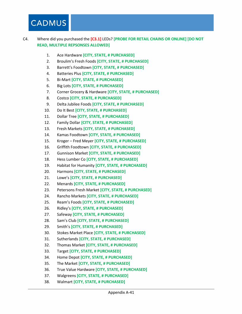
Appendix A-41
C4. Where did you purchased the [C3.1] LEDs? [PROBE FOR RETAIL CHAINS OR ONLINE] [DO NOT
READ, MULTIPLE REPSONSES ALLOWED]
1. Ace Hardware [CITY, STATE, # PURCHASED]
2. Broulim’s Fresh Foods [CITY, STATE, # PURCHASED]
3. Barrett’s Foodtown [CITY, STATE, # PURCHASED]
4. Batteries Plus [CITY, STATE, # PURCHASED]
5. Bi-Mart [CITY, STATE, # PURCHASED]
6. Big Lots [CITY, STATE, # PURCHASED]
7. Corner Grocery & Hardware [CITY, STATE, # PURCHASED]
8. Costco [CITY, STATE, # PURCHASED]
9. Delta Jubilee Foods [CITY, STATE, # PURCHASED]
10. Do It Best [CITY, STATE, # PURCHASED]
11. Dollar Tree [CITY, STATE, # PURCHASED]
12. Family Dollar [CITY, STATE, # PURCHASED]
13. Fresh Markets [CITY, STATE, # PURCHASED]
14. Kamas Foodtown [CITY, STATE, # PURCHASED]
15. Kroger – Fred Meyer [CITY, STATE, # PURCHASED]
16. Griffith Foodtown [CITY, STATE, # PURCHASED]
17. Gunnison Market [CITY, STATE, # PURCHASED]
18. Hess Lumber Co [CITY, STATE, # PURCHASED]
19. Habitat for Humanity [CITY, STATE, # PURCHASED]
20. Harmons [CITY, STATE, # PURCHASED]
21. Lowe’s [CITY, STATE, # PURCHASED]
22. Menards [CITY, STATE, # PURCHASED]
23. Petersons Fresh Market [CITY, STATE, # PURCHASED]
24. Rancho Markets [CITY, STATE, # PURCHASED]
25. Ream’s Foods [CITY, STATE, # PURCHASED]
26. Ridley’s [CITY, STATE, # PURCHASED]
27. Safeway [CITY, STATE, # PURCHASED]
28. Sam’s Club [CITY, STATE, # PURCHASED]
29. Smith’s [CITY, STATE, # PURCHASED]
30. Stokes Market Place [CITY, STATE, # PURCHASED]
31. Sutherlands [CITY, STATE, # PURCHASED]
32. Thomas Market [CITY, STATE, # PURCHASED]
33. Target [CITY, STATE, # PURCHASED]
34. Home Depot [CITY, STATE, # PURCHASED]
35. The Market [CITY, STATE, # PURCHASED]
36. True Value Hardware [CITY, STATE, # PURCHASED]
37. Walgreens [CITY, STATE, # PURCHASED]
38. Walmart [CITY, STATE, # PURCHASED]
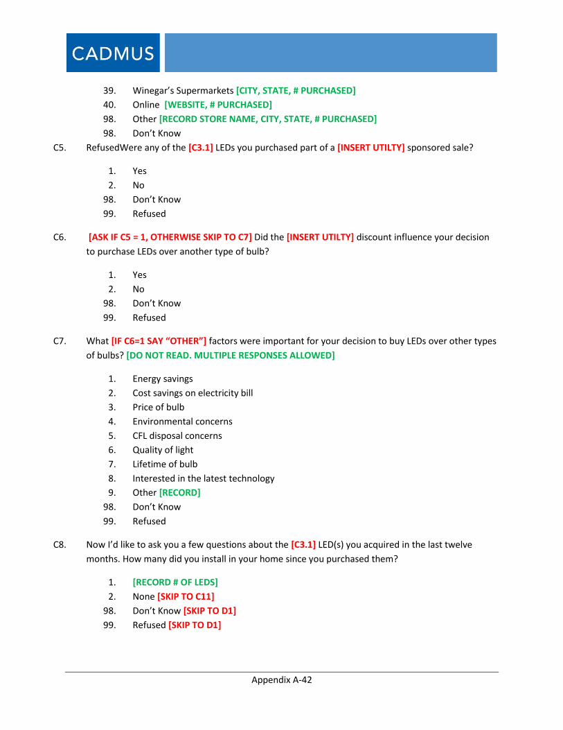
Appendix A-42
39. Winegar’s Supermarkets [CITY, STATE, # PURCHASED]
40. Online [WEBSITE, # PURCHASED]
98. Other [RECORD STORE NAME, CITY, STATE, # PURCHASED]
98. Don’t Know
C5. RefusedWere any of the [C3.1] LEDs you purchased part of a [INSERT UTILTY] sponsored sale?
1. Yes
2. No
98. Don’t Know
99. Refused
C6. [ASK IF C5 = 1, OTHERWISE SKIP TO C7] Did the [INSERT UTILTY] discount influence your decision
to purchase LEDs over another type of bulb?
1. Yes
2. No
98. Don’t Know
99. Refused
C7. What [IF C6=1 SAY “OTHER”] factors were important for your decision to buy LEDs over other types
of bulbs? [DO NOT READ. MULTIPLE RESPONSES ALLOWED]
1. Energy savings
2. Cost savings on electricity bill
3. Price of bulb
4. Environmental concerns
5. CFL disposal concerns
6. Quality of light
7. Lifetime of bulb
8. Interested in the latest technology
9. Other [RECORD]
98. Don’t Know
99. Refused
C8. Now I’d like to ask you a few questions about the [C3.1] LED(s) you acquired in the last twelve
months. How many did you install in your home since you purchased them?
1. [RECORD # OF LEDS]
2. None [SKIP TO C11]
98. Don’t Know [SKIP TO D1]
99. Refused [SKIP TO D1]
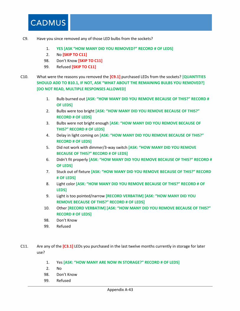
Appendix A-43
C9. Have you since removed any of those LED bulbs from the sockets?
1. YES [ASK “HOW MANY DID YOU REMOVED?” RECORD # OF LEDS]
2. No [SKIP TO C11]
98. Don’t Know [SKIP TO C11]
99. Refused [SKIP TO C11]
C10. What were the reasons you removed the [C9.1] purchased LEDs from the sockets? [QUANTITIES
SHOULD ADD TO B10.1, IF NOT, ASK “WHAT ABOUT THE REMAINING BULBS YOU REMOVED?]
[DO NOT READ, MULTIPLE RESPONSES ALLOWED]
1. Bulb burned out [ASK: “HOW MANY DID YOU REMOVE BECAUSE OF THIS?” RECORD #
OF LEDS]
2. Bulbs were too bright [ASK: “HOW MANY DID YOU REMOVE BECAUSE OF THIS?”
RECORD # OF LEDS]
3. Bulbs were not bright enough [ASK: “HOW MANY DID YOU REMOVE BECAUSE OF
THIS?” RECORD # OF LEDS]
4. Delay in light coming on [ASK: “HOW MANY DID YOU REMOVE BECAUSE OF THIS?”
RECORD # OF LEDS]
5. Did not work with dimmer/3-way switch [ASK: “HOW MANY DID YOU REMOVE
BECAUSE OF THIS?” RECORD # OF LEDS]
6. Didn’t fit properly [ASK: “HOW MANY DID YOU REMOVE BECAUSE OF THIS?” RECORD #
OF LEDS]
7. Stuck out of fixture [ASK: “HOW MANY DID YOU REMOVE BECAUSE OF THIS?” RECORD
# OF LEDS]
8. Light color [ASK: “HOW MANY DID YOU REMOVE BECAUSE OF THIS?” RECORD # OF
LEDS]
9. Light is too pointed/narrow [RECORD VERBATIM] [ASK: “HOW MANY DID YOU
REMOVE BECAUSE OF THIS?” RECORD # OF LEDS]
10. Other [RECORD VERBATIM] [ASK: “HOW MANY DID YOU REMOVE BECAUSE OF THIS?”
RECORD # OF LEDS]
98. Don’t Know
99. Refused
C11. Are any of the [C3.1] LEDs you purchased in the last twelve months currently in storage for later
use?
1. Yes [ASK: “HOW MANY ARE NOW IN STORAGE?” RECORD # OF LEDS]
2. No
98. Don’t Know
99. Refused

Appendix A-44
C12. [SKIP TO C14 IF C8= 2, 99, OR 98] Of the [C8.1] bulbs that are currently installed in your home that
were purchased during the last twelve months, can you tell me how many LEDs are installed in each
room in your house?
1. Bedroom [RECORD]
2. Bedroom (unoccupied) [RECORD]
3. Basement [RECORD]
4. Bathroom [RECORD]
5. Closet [RECORD]
6. Dining [RECORD]
7. Foyer [RECORD]
8. Garage [RECORD]
9. Hallway [RECORD]
10. Kitchen [RECORD]
11. Office/Den [RECORD]
12. Living Space [RECORD]
13. Storage [RECORD]
14. Outdoor [RECORD]
15. Utility [RECORD]
16. Other [RECORD VERBATIM]
98. Don’t Know
99. Refused
C13. [ASK ONLY IF TOTAL BULBS IN C12<C8.1 (IF TOTAL NUMBER OF BULBS LISTED IN EACH ROOM
DOES NOT MATCH THE NUMBER OF BULBS INSTALLED STATED IN C8.1)OTHERWISE SKIP TO C13]
Thanks, that accounts for [TOTAL BULBS IN C12] of the total quantity that were installed in your
home. Can you tell me where the [C8.1 MINUS TOTAL BULBS IN C12] other bulbs were installed?
1. [RECORD VERBATIM]
98. Don’t Know
99. Refused
C14. How satisfied are you with the LEDs that you purchased during the last twelve months? Would you
say you are… [READ]
1. Very Satisfied
2. Somewhat Satisfied
3. Not Very Satisfied
4. Not At All Satisfied
98. [DO NOT READ] Don’t Know
99. [DO NOT READ] Refused
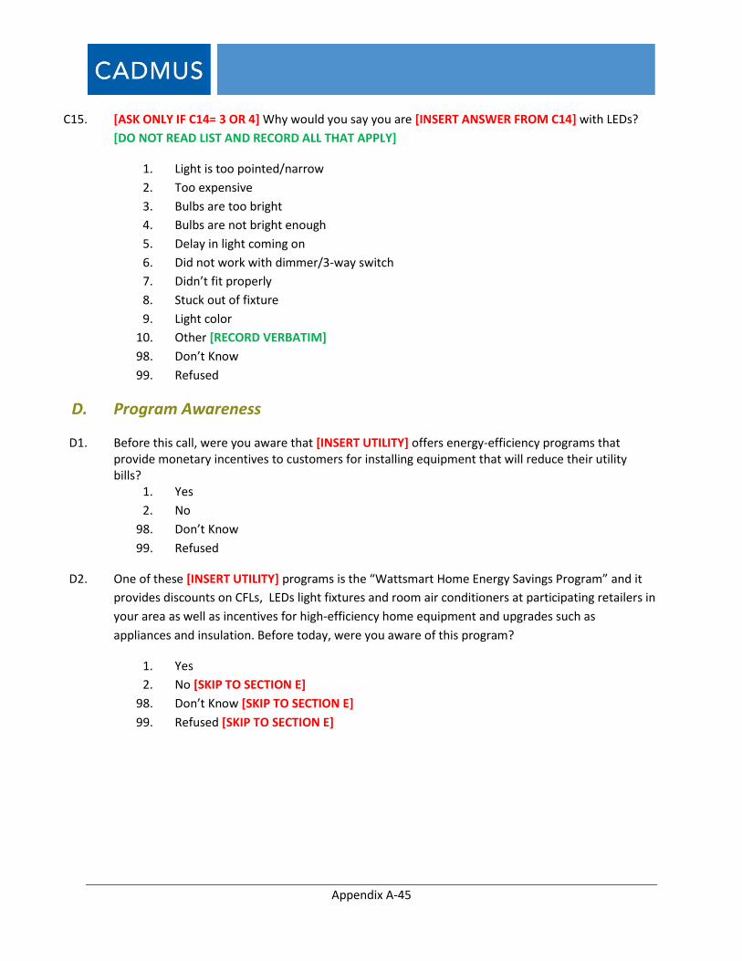
Appendix A-45
C15. [ASK ONLY IF C14= 3 OR 4] Why would you say you are [INSERT ANSWER FROM C14] with LEDs?
[DO NOT READ LIST AND RECORD ALL THAT APPLY]
1. Light is too pointed/narrow
2. Too expensive
3. Bulbs are too bright
4. Bulbs are not bright enough
5. Delay in light coming on
6. Did not work with dimmer/3-way switch
7. Didn’t fit properly
8. Stuck out of fixture
9. Light color
10. Other [RECORD VERBATIM]
98. Don’t Know
99. Refused
D. Program Awareness
D1. Before this call, were you aware that [INSERT UTILITY] offers energy-efficiency programs that provide monetary incentives to customers for installing equipment that will reduce their utility bills?
1. Yes
2. No
98. Don’t Know
99. Refused
D2. One of these [INSERT UTILITY] programs is the “Wattsmart Home Energy Savings Program” and it
provides discounts on CFLs, LEDs light fixtures and room air conditioners at participating retailers in
your area as well as incentives for high-efficiency home equipment and upgrades such as
appliances and insulation. Before today, were you aware of this program?
1. Yes
2. No [SKIP TO SECTION E]
98. Don’t Know [SKIP TO SECTION E]
99. Refused [SKIP TO SECTION E]
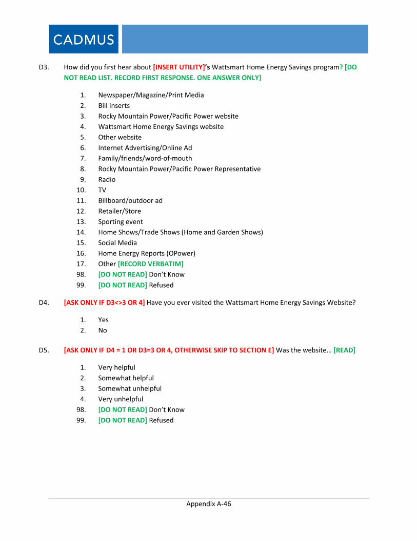
Appendix A-46
D3. How did you first hear about [INSERT UTILITY]’s Wattsmart Home Energy Savings program? [DO
NOT READ LIST. RECORD FIRST RESPONSE. ONE ANSWER ONLY]
1. Newspaper/Magazine/Print Media
2. Bill Inserts
3. Rocky Mountain Power/Pacific Power website
4. Wattsmart Home Energy Savings website
5. Other website
6. Internet Advertising/Online Ad
7. Family/friends/word-of-mouth
8. Rocky Mountain Power/Pacific Power Representative
9. Radio
10. TV
11. Billboard/outdoor ad
12. Retailer/Store
13. Sporting event
14. Home Shows/Trade Shows (Home and Garden Shows)
15. Social Media
16. Home Energy Reports (OPower)
17. Other [RECORD VERBATIM]
98. [DO NOT READ] Don’t Know
99. [DO NOT READ] Refused
D4. [ASK ONLY IF D3<>3 OR 4] Have you ever visited the Wattsmart Home Energy Savings Website?
1. Yes
2. No
D5. [ASK ONLY IF D4 = 1 OR D3=3 OR 4, OTHERWISE SKIP TO SECTION E] Was the website… [READ]
1. Very helpful
2. Somewhat helpful
3. Somewhat unhelpful
4. Very unhelpful
98. [DO NOT READ] Don’t Know
99. [DO NOT READ] Refused
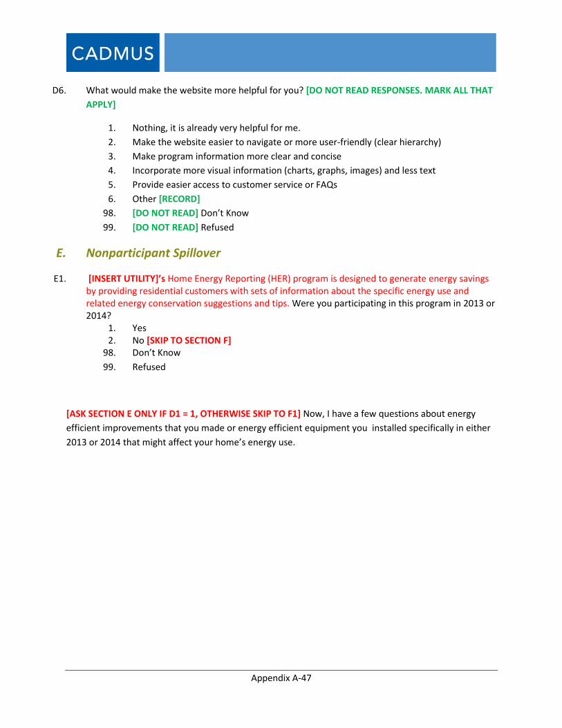
Appendix A-47
D6. What would make the website more helpful for you? [DO NOT READ RESPONSES. MARK ALL THAT
APPLY]
1. Nothing, it is already very helpful for me.
2. Make the website easier to navigate or more user-friendly (clear hierarchy)
3. Make program information more clear and concise
4. Incorporate more visual information (charts, graphs, images) and less text
5. Provide easier access to customer service or FAQs
6. Other [RECORD]
98. [DO NOT READ] Don’t Know
99. [DO NOT READ] Refused
E. Nonparticipant Spillover
E1. [INSERT UTILITY]’s Home Energy Reporting (HER) program is designed to generate energy savings by providing residential customers with sets of information about the specific energy use and related energy conservation suggestions and tips. Were you participating in this program in 2013 or 2014?
1. Yes 2. No [SKIP TO SECTION F]
98. Don’t Know
99. Refused
[ASK SECTION E ONLY IF D1 = 1, OTHERWISE SKIP TO F1] Now, I have a few questions about energy
efficient improvements that you made or energy efficient equipment you installed specifically in either
2013 or 2014 that might affect your home’s energy use.
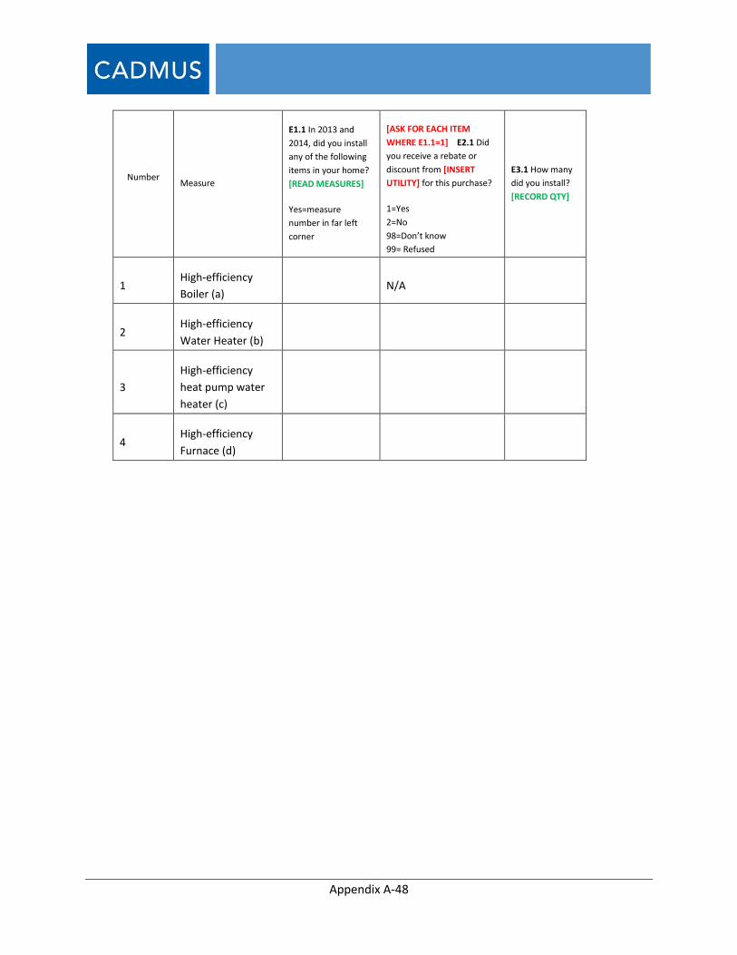
Appendix A-48
Number Measure
E1.1 In 2013 and
2014, did you install
any of the following
items in your home?
[READ MEASURES]
Yes=measure
number in far left
corner
[ASK FOR EACH ITEM
WHERE E1.1=1] E2.1 Did
you receive a rebate or
discount from [INSERT
UTILITY] for this purchase?
1=Yes
2=No
98=Don’t know
99= Refused
E3.1 How many
did you install?
[RECORD QTY]
1 High-efficiency
Boiler (a) N/A
2 High-efficiency
Water Heater (b)
3
High-efficiency
heat pump water
heater (c)
4 High-efficiency
Furnace (d)
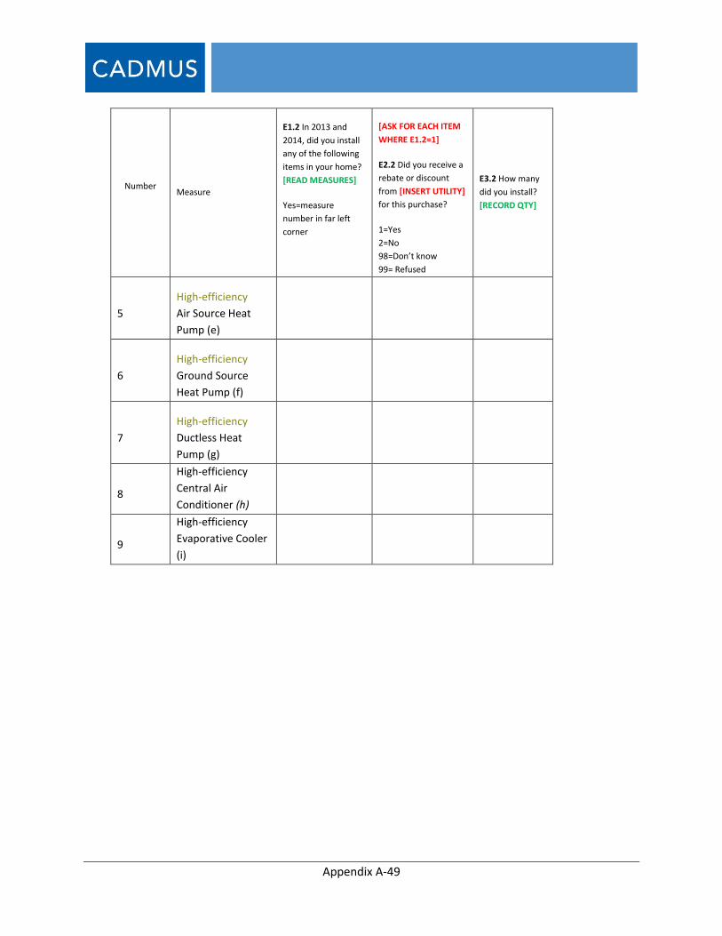
Appendix A-49
Number Measure
E1.2 In 2013 and
2014, did you install
any of the following
items in your home?
[READ MEASURES]
Yes=measure
number in far left
corner
[ASK FOR EACH ITEM
WHERE E1.2=1]
E2.2 Did you receive a
rebate or discount
from [INSERT UTILITY]
for this purchase?
1=Yes
2=No
98=Don’t know
99= Refused
E3.2 How many
did you install?
[RECORD QTY]
5
High-efficiency
Air Source Heat
Pump (e)
6
High-efficiency
Ground Source
Heat Pump (f)
7
High-efficiency
Ductless Heat
Pump (g)
8
High-efficiency
Central Air
Conditioner (h)
9
High-efficiency
Evaporative Cooler
(i)

Appendix A-50
Number Measure
E1.3 In 2013 and
2014, did you install
any of the following
items in your home?
[READ MEASURES]
Yes=measure
number in far left
corner
[ASK FOR EACH ITEM
WHERE E1.3=1]
E2.3 Did you receive a
rebate or discount
from [INSERT UTILITY]
for this purchase?
1=Yes
2=No
98=Don’t know
99= Refused
E3.3 How many
did you install?
[RECORD QTY]
10 ENEGY STAR Room
Air Conditioner (j)
11 ENERGY STAR
Clothes Washer (k)
12 ENERGY STAR
Dishwasher (l)
13 ENERGY STAR
Freezer (m)
14 ENERGY STAR
Refrigerator (n)
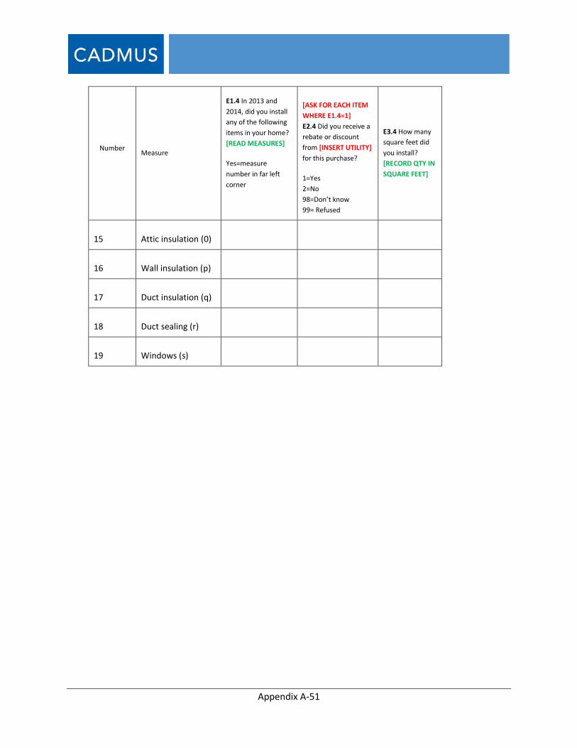
Appendix A-51
Number Measure
E1.4 In 2013 and
2014, did you install
any of the following
items in your home?
[READ MEASURES]
Yes=measure
number in far left
corner
[ASK FOR EACH ITEM
WHERE E1.4=1]
E2.4 Did you receive a
rebate or discount
from [INSERT UTILITY]
for this purchase?
1=Yes
2=No
98=Don’t know
99= Refused
E3.4 How many
square feet did
you install?
[RECORD QTY IN
SQUARE FEET]
15 Attic insulation (0)
16 Wall insulation (p)
17 Duct insulation (q)
18 Duct sealing (r)
19 Windows (s)
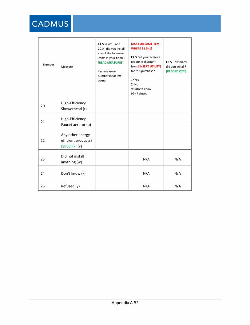
Appendix A-52
Number Measure
E1.5 In 2013 and
2014, did you install
any of the following
items in your home?
[READ MEASURES]
Yes=measure
number in far left
corner
[ASK FOR EACH ITEM
WHERE E1.5=1]
E2.5 Did you receive a
rebate or discount
from [INSERT UTILITY]
for this purchase?
1=Yes
2=No
98=Don’t know
99= Refused
E3.5 How many
did you install?
[RECORD QTY]
20 High-Efficiency
Showerhead (t)
21 High-Efficiency
Faucet aerator (u)
22
Any other energy-
efficient products?
[SPECIFY] (v)
23 Did not install
anything (w) N/A N/A
24 Don’t know (x) N/A N/A
25 Refused (y) N/A N/A
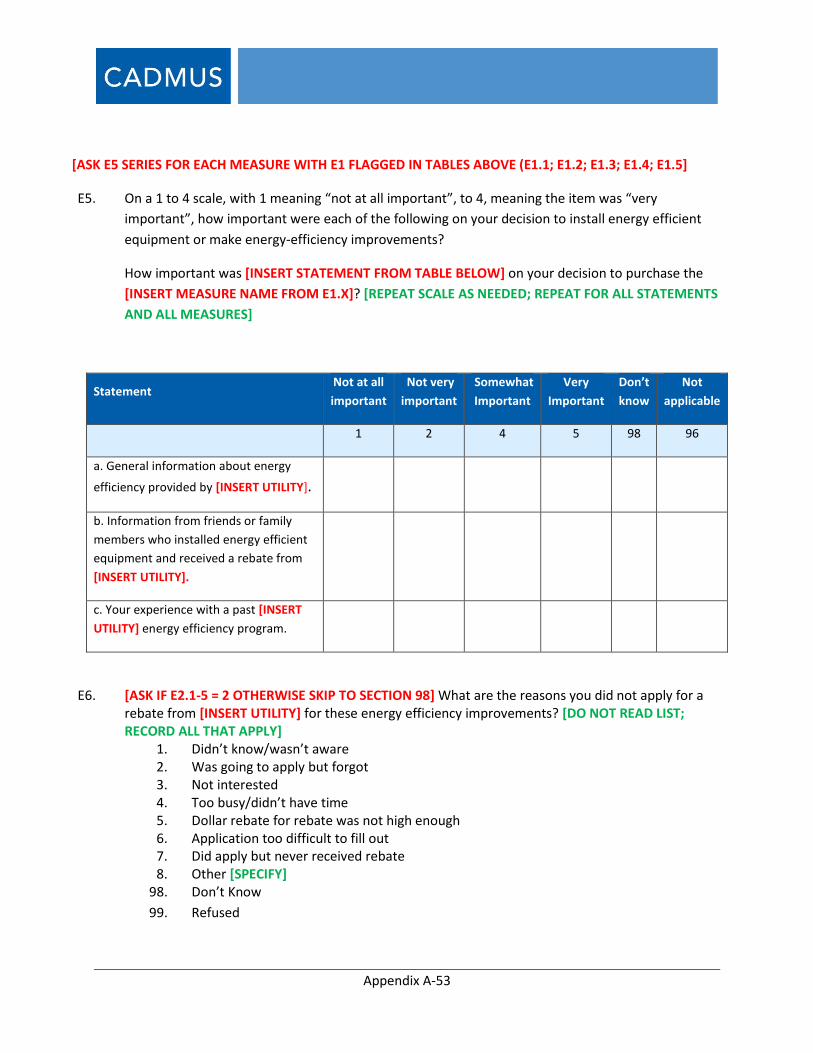
Appendix A-53
[ASK E5 SERIES FOR EACH MEASURE WITH E1 FLAGGED IN TABLES ABOVE (E1.1; E1.2; E1.3; E1.4; E1.5]
E5. On a 1 to 4 scale, with 1 meaning “not at all important”, to 4, meaning the item was “very
important”, how important were each of the following on your decision to install energy efficient
equipment or make energy-efficiency improvements?
How important was [INSERT STATEMENT FROM TABLE BELOW] on your decision to purchase the
[INSERT MEASURE NAME FROM E1.X]? [REPEAT SCALE AS NEEDED; REPEAT FOR ALL STATEMENTS
AND ALL MEASURES]
Statement Not at all
important
Not very
important
Somewhat
Important
Very
Important
Don’t
know
Not
applicable
1 2 4 5 98 96
a. General information about energy
efficiency provided by [INSERT UTILITY].
b. Information from friends or family
members who installed energy efficient
equipment and received a rebate from
[INSERT UTILITY].
c. Your experience with a past [INSERT
UTILITY] energy efficiency program.
E6. [ASK IF E2.1-5 = 2 OTHERWISE SKIP TO SECTION 98] What are the reasons you did not apply for a rebate from [INSERT UTILITY] for these energy efficiency improvements? [DO NOT READ LIST; RECORD ALL THAT APPLY]
1. Didn’t know/wasn’t aware 2. Was going to apply but forgot 3. Not interested 4. Too busy/didn’t have time 5. Dollar rebate for rebate was not high enough 6. Application too difficult to fill out 7. Did apply but never received rebate 8. Other [SPECIFY]
98. Don’t Know
99. Refused
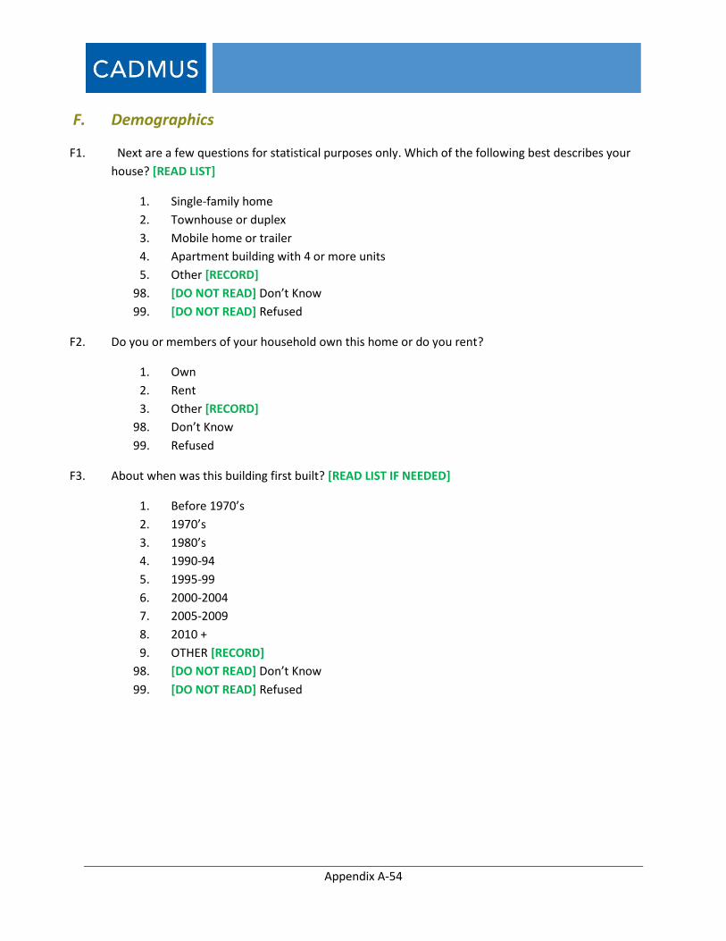
Appendix A-54
F. Demographics
F1. Next are a few questions for statistical purposes only. Which of the following best describes your
house? [READ LIST]
1. Single-family home
2. Townhouse or duplex
3. Mobile home or trailer
4. Apartment building with 4 or more units
5. Other [RECORD]
98. [DO NOT READ] Don’t Know
99. [DO NOT READ] Refused
F2. Do you or members of your household own this home or do you rent?
1. Own
2. Rent
3. Other [RECORD]
98. Don’t Know
99. Refused
F3. About when was this building first built? [READ LIST IF NEEDED]
1. Before 1970’s
2. 1970’s
3. 1980’s
4. 1990-94
5. 1995-99
6. 2000-2004
7. 2005-2009
8. 2010 +
9. OTHER [RECORD]
98. [DO NOT READ] Don’t Know
99. [DO NOT READ] Refused
Appendix A-55
F4. What is the primary heating source for your home? [READ LIST IF NEEDED]
1. Forced air natural gas furnace
2. Forced air propane furnace
3. Air Source Heat Pump [FUEL SOURCE]
4. Ground Source Heat Pump [FUEL SOURCE]
5. Electric baseboard heat
6. Gas fired boiler/radiant heat
7. Oil fired boiler/radiant heat
8. Passive Solar
9. Pellet stove
10. Wood stove
11. Other [RECORD]
98. Don’t Know
99. Refused
F5. How old is the primary heating system? [RECORD RESPONSE IN YEARS]
1. [RECORD 1-100]
98. Don’t Know
99. Refused
F6. What type of air conditioning system, if any, do you use in your home? [INDICATE ALL THAT
APPLY]
1. Central Air Conditioner
2. Room Air Conditioner
3. Evaporative Cooler
4. Air Source Heat Pump
5. Ground Source Heat Pump
6. Whole house fan
7. No cooling system
8. Other [SPECIFY]
98. [DO NOT READ] Don’t Know
99. [DO NOT READ] Refused
F7. [SKIP IF F6= 7,98 OR 99] How many years old is your primary cooling system? [RECORD RESPONSE
IN YEARS]
1. [RECORD]
98. Don’t Know
99. Refused
Appendix A-56
F8. What type of fuel is the primary source for your water heating? [INDICATE ALL THAT APPLY]
1. Electricity
2. Natural Gas
3. Propane
4. Other [RECORD]
98. [DO NOT READ] Don’t Know
99. [DO NOT READ] Refused
F9. Including yourself and any children, how many people currently live in your home?
1. [RECORD]
98. Don’t Know
99. Refused
F10. [ASK ONLY IF F9> 1] Are any of the people living in your home dependent children under the age of
18?
1. Yes
2. No
98. Don’t Know
99. Refused
G. Conclusion
G1. Do you have any additional feedback or comments regarding your household lighting?
1. Yes [RECORD VERBATIM]
2. No
98. Don’t Know
99. Refused
G2. [SEX; DO NOT READ]
1. Female
2. Male
98. Don’t Know
That concludes the survey. Thank you very much for your time and feedback.
A-57
Appendix A: Lighting Leakage Survey A1 Hello, my name is _____, and we’re doing a survey about light bulbs today. This is a short survey that
will only take about five minutes to complete, and we will give you a $10 gift card that you can use in
this store today for your time. You will remain completely anonymous. Do you have five minutes to
answer some questions today?
1. (Yes) (1)
99. (No/Refused) (2)
If 1. (Yes) Is Selected, Then Skip To A3
If 99. (No/Refused) Is Selected
A2 OK, thanks for your consideration. Though if you don’t mind answering one question for me, could
you please tell me which utility provides electric service to your home? [SHOW UTILITY LOGOS IF
NEEDED. THANK THE CUSTOMER AND END SURVEY AFTER THIS QUESTION]
1. Pacific Power (1)
2. Rocky Mountain Power (2)
91. Any other utility (specify) (3) ____________________
98. Don't know (4) 99. Refused (5)
Then Skip To E1 short A3 Which utility provides electric service to your home? [SHOW UTILITY LOGOS IF NEEDED] 1. Pacific Power (1) 2. Rocky Mountain Power (2) 91. Any other utility (specify) (3) ____________________ 98. Don't know (4) 99. Refused (5)
A-58
A4 Which zip code do you live in? Record response if given (1) ____________________ 98. Don't know (2) 99. Refused (3) B1 Do you plan to install the bulbs you’re purchasing today in your home, at a business, or someplace else? [CHECK ALL THAT APPLY – ONLY CHECK ONE IF ALL BULBS ARE BEING INSTALLED AT THE SAME ADDRESS] 1. (bulbs will be installed at my home) (1)
2. (bulbs will be installed at my vacation home (or other personal property) (2)
3. (bulbs will be installed at a business / location that is not a residence, including non-profits) (3)
4. (purchasing bulbs for somebody else / not my home or business) (4)
98. (Don’t know) (5)
99. (Refused) (6)
If (bulbs will be installed at a business / location that is not a residence, including non-profits) Is Selected
B1a What kind of business is this (what do they do)?
A: AGRICULTURE, FORESTRY AND FISHING (VETERINARY, CROPS, HUNTING) (1)
B: MINING (GRAVEL, COAL, OIL, METAL, CHEMICAL, NONMETALLIC MINERALS) (2)
C: CONTRACT CONSTRUCTION (PLUMBING, PAINTING, ELECTRICAL, ROOFING) (3)
D: MANUFACTURING (TEXTILES, FURNITURE, FABRICATED METAL, PRODUCTS) (4)
E: TRANSPORTATION, COMMUNICATION, ELECTRIC (FREIGHT, COURIER, CABLE) (5)
F: WHOLESALE TRADE (GROCERY SUPPLIERS, RAW MATERIALS, APPAREL) (6)
G: RETAIL TRADE (MARKETS, CLOTHING STORES, RESTAURANTS, CAR DEALERS) (7)
H: FINANCE, INSURANCE AND REAL ESTATE (BANKS, MORTGAGE BROKERS) (8)
I: SERVICES (BEAUTY QUALITY) (9)
K: NONCLASSIFIABLE ESTABLISHMENTS (OTHERS) [RECORD RESPONSE] (10) ____________________
(98. don't know) (11)
(99. refused) (12)
A-59
If (bulbs will be installed at a business / location that is not a residence, including non-profits) Is Selected
B1b What zip code or city is this business located in? [RECORD ZIP CODE IF KNOWN]
(RECORD RESPONSE IF GIVEN) (1) ____________________
(98. don't know) (2)
(99. refused) (3)
If (bulbs will be installed at a business / location that is not a residence, including non-profits) Is Selected
B1c Do you know which utility provides power for this business? [RECORD NAME OF UTILITY IF KNOWN]
(1. Pacific Power) (1)
(2. Rocky Mountain Power) (2)
(3. Any other utility - SPECIFY) (3) ____________________
(98. don't know) (4)
(99. refused) (5)
If (purchasing bulbs for somebody else / not my home or business) Is Selected
B1d Do you know where these bulbs that you are purchasing for somebody else will be installed? (Do
you know the zip code or city?) [RECORD RESPONSE – ZIP CODE IS IDEAL, OR CITY AND STATE, OR JUST A
VERBAL DESCRIPTION IF ADDRESS IS NOT KNOWN – for example “my mother-in-law’s house”]
(1. RECORD RESPONSE IF GIVEN) (1) ____________________
(98. don't know) (2)
(99. refused) (3)
B2 How many minutes does it take to drive to this store from the place where you intend to install these
bulbs?
(Less than 10 minutes) (1)
(10 up to 20 minutes) (2)
(20 up to 30 minutes) (3)
(30 up to 40 minutes) (4)
(40 up to 50 minutes) (5)
(50 minutes up to an hour) (6)
(An hour or more) (7)
(Other response or multiple locations - record details below) (8) ____________________
(98. don't know) (9)
(99. refused) (10)
A-60
B3 What kind of light bulbs are you purchasing today? [GO OVER THE LIGHT BULBS IN THE CUSTOMER’S
CART AND RECORD HOW MANY OF EACH TYPE – ONLY CONTINUE IF THERE IS AT LEAST ONE LIGHT BULB
IN THEIR CART.]
(Enter quantity of INCANDESCENT bulbs) (1) ____________________
(Enter quantity of HALOGEN bulbs) (2) ____________________
(Enter quantity of CFL bulbs) (3) ____________________
(Enter quantity of LED bulbs) (4) ____________________
(Enter quantity AND TYPE of OTHER bulbs) (5) ____________________
B3scan [SCAN THE BARCODES FOR THE LIGHT BULBS IN THEIR CART AND COPY-PASTE THE
NUMBERS INTO THE FIELDS BELOW - ONLY NEED TO SCAN ONE PACKAGE OF EACH TYPE OR WATTAGE;
DO NOT SCAN MULTIPLE PACKS OF EXACTLY THE SAME BULBS.]
First light bulb type (1) ____________________
Second light bulb type (2) ____________________
Third light bulb type (3) ____________________
Fourth light bulb type (4) ____________________
Fifth light bulb type (5) ____________________
Sixth light bulb type (6) ____________________
Seventh light bulb type (7) ____________________
Eighth light bulb type (8) ____________________
If (Enter quantity of INCANDESCENT bulbs) Is Greater Than or Equal to 1
B3i What type and wattage of light bulb will you replace with the INCANDESCENT bulbs you are
purchasing today?
(1. Incandescent bulbs) RECORD WATTAGE(S) IF KNOWN (1) ____________________
(2. Halogen bulbs) RECORD WATTAGE(S) IF KNOWN (2) ____________________
(3. CFL bulbs) RECORD WATTAGE(S) IF KNOWN (3) ____________________
(4. LED bulbs) RECORD WATTAGE(S) IF KNOWN (4) ____________________
(5. other type of bulbs) RECORD TYPE AND WATTAGE(S) IF KNOWN (5) ____________________
(6. purchasing bulbs for general use / that will go in storage / not specifically replacing any particular
bulbs) (6)
(7. no bulbs previously installed / new fixture or previously empty sockets) (7)
(98. don't know) (8)
(99. refused) (9)
A-61
If (Enter quantity of HALOGEN bulbs) Is Greater Than or Equal to 1
B3h What type and wattage of light bulb will you replace with the HALOGEN bulbs you are purchasing
today?
(1. Incandescent bulbs) RECORD WATTAGE(S) IF KNOWN (1) ____________________
(2. Halogen bulbs) RECORD WATTAGE(S) IF KNOWN (2) ____________________
(3. CFL bulbs) RECORD WATTAGE(S) IF KNOWN (3) ____________________
(4. LED bulbs) RECORD WATTAGE(S) IF KNOWN (4) ____________________
(5. other type of bulbs) RECORD TYPE AND WATTAGE(S) IF KNOWN (5) ____________________
(6. purchasing bulbs for general use / that will go in storage / not specifically replacing any particular
bulbs) (6)
(7. no bulbs previously installed / new fixture or previously empty sockets) (7)
(98. don't know) (8)
(99. refused) (9)
A-62
If (Enter quantity of CFL bulbs) Is Greater Than or Equal to 1
B3c What type and wattage of light bulb will you replace with the CFL bulbs you are purchasing today?
(1. Incandescent bulbs) RECORD WATTAGE(S) IF KNOWN (1) ____________________
(2. Halogen bulbs) RECORD WATTAGE(S) IF KNOWN (2) ____________________
(3. CFL bulbs) RECORD WATTAGE(S) IF KNOWN (3) ____________________
(4. LED bulbs) RECORD WATTAGE(S) IF KNOWN (4) ____________________
(5. other type of bulbs) RECORD TYPE AND WATTAGE(S) IF KNOWN (5) ____________________
(6. purchasing bulbs for general use / that will go in storage / not specifically replacing any particular
bulbs) (6)
(7. no bulbs previously installed / new fixture or previously empty sockets) (7)
(98. don't know) (8)
(99. refused) (9)
If (Enter quantity of LED bulbs) Is Greater Than or Equal to 1
B3l What type and wattage of light bulb will you replace with the LED bulbs you are purchasing today?
(1. Incandescent bulbs) RECORD WATTAGE(S) IF KNOWN (1) ____________________
(2. Halogen bulbs) RECORD WATTAGE(S) IF KNOWN (2) ____________________
(3. CFL bulbs) RECORD WATTAGE(S) IF KNOWN (3) ____________________
(4. LED bulbs) RECORD WATTAGE(S) IF KNOWN (4) ____________________
(5. other type of bulbs) RECORD TYPE AND WATTAGE(S) IF KNOWN (5) ____________________
(6. purchasing bulbs for general use / that will go in storage / not specifically replacing any particular
bulbs) (6)
(7. no bulbs previously installed / new fixture or previously empty sockets) (7)
(98. don't know) (8)
(99. refused) (9)
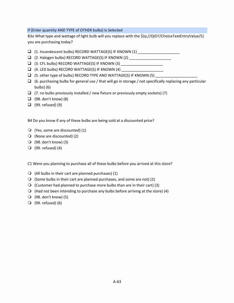
A-63
If (Enter quantity AND TYPE of OTHER bulbs) Is Selected
B3o What type and wattage of light bulb will you replace with the ${q://QID7/ChoiceTextEntryValue/5}
you are purchasing today?
(1. Incandescent bulbs) RECORD WATTAGE(S) IF KNOWN (1) ____________________
(2. Halogen bulbs) RECORD WATTAGE(S) IF KNOWN (2) ____________________
(3. CFL bulbs) RECORD WATTAGE(S) IF KNOWN (3) ____________________
(4. LED bulbs) RECORD WATTAGE(S) IF KNOWN (4) ____________________
(5. other type of bulbs) RECORD TYPE AND WATTAGE(S) IF KNOWN (5) ____________________
(6. purchasing bulbs for general use / that will go in storage / not specifically replacing any particular
bulbs) (6)
(7. no bulbs previously installed / new fixture or previously empty sockets) (7)
(98. don't know) (8)
(99. refused) (9)
B4 Do you know if any of these bulbs are being sold at a discounted price?
(Yes, some are discounted) (1)
(None are discounted) (2)
(98. don't know) (3)
(99. refused) (4)
C1 Were you planning to purchase all of these bulbs before you arrived at this store?
(All bulbs in their cart are planned purchases) (1)
(Some bulbs in their cart are planned purchases, and some are not) (2)
(Customer had planned to purchase more bulbs than are in their cart) (3)
(Had not been intending to purchase any bulbs before arriving at the store) (4)
(98. don't know) (5)
(99. refused) (6)
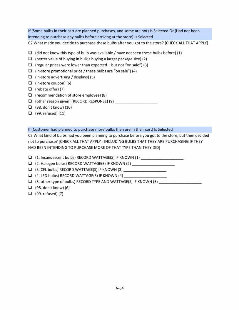
A-64
If (Some bulbs in their cart are planned purchases, and some are not) Is Selected Or (Had not been
intending to purchase any bulbs before arriving at the store) Is Selected
C2 What made you decide to purchase these bulbs after you got to the store? [CHECK ALL THAT APPLY]
(did not know this type of bulb was available / have not seen these bulbs before) (1)
(better value of buying in bulk / buying a larger package size) (2)
(regular prices were lower than expected – but not “on sale”) (3)
(in-store promotional price / these bulbs are “on sale”) (4)
(in-store advertising / displays) (5)
(in-store coupon) (6)
(rebate offer) (7)
(recommendation of store employee) (8)
(other reason given) [RECORD RESPONSE] (9) ____________________
(98. don't know) (10)
(99. refused) (11)
If (Customer had planned to purchase more bulbs than are in their cart) Is Selected
C3 What kind of bulbs had you been planning to purchase before you got to the store, but then decided
not to purchase? [CHECK ALL THAT APPLY - INCLUDING BULBS THAT THEY ARE PURCHASING IF THEY
HAD BEEN INTENDING TO PURCHASE MORE OF THAT TYPE THAN THEY DID]
(1. Incandescent bulbs) RECORD WATTAGE(S) IF KNOWN (1) ____________________
(2. Halogen bulbs) RECORD WATTAGE(S) IF KNOWN (2) ____________________
(3. CFL bulbs) RECORD WATTAGE(S) IF KNOWN (3) ____________________
(4. LED bulbs) RECORD WATTAGE(S) IF KNOWN (4) ____________________
(5. other type of bulbs) RECORD TYPE AND WATTAGE(S) IF KNOWN (5) ____________________
(98. don't know) (6)
(99. refused) (7)
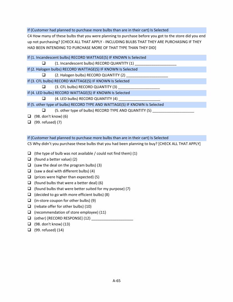
A-65
If (Customer had planned to purchase more bulbs than are in their cart) Is Selected
C4 How many of these bulbs that you were planning to purchase before you got to the store did you end
up not purchasing? [CHECK ALL THAT APPLY - INCLUDING BULBS THAT THEY ARE PURCHASING IF THEY
HAD BEEN INTENDING TO PURCHASE MORE OF THAT TYPE THAN THEY DID]
If (1. Incandescent bulbs) RECORD WATTAGE(S) IF KNOWN Is Selected
(1. Incandescent bulbs) RECORD QUANTITY (1) ____________________
If (2. Halogen bulbs) RECORD WATTAGE(S) IF KNOWN Is Selected
(2. Halogen bulbs) RECORD QUANTITY (2) ____________________
If (3. CFL bulbs) RECORD WATTAGE(S) IF KNOWN Is Selected
(3. CFL bulbs) RECORD QUANTITY (3) ____________________
If (4. LED bulbs) RECORD WATTAGE(S) IF KNOWN Is Selected
(4. LED bulbs) RECORD QUANTITY (4) ____________________
If (5. other type of bulbs) RECORD TYPE AND WATTAGE(S) IF KNOWN Is Selected
(5. other type of bulbs) RECORD TYPE AND QUANTITY (5) ____________________
(98. don't know) (6)
(99. refused) (7)
If (Customer had planned to purchase more bulbs than are in their cart) Is Selected
C5 Why didn’t you purchase these bulbs that you had been planning to buy? [CHECK ALL THAT APPLY]
(the type of bulb was not available / could not find them) (1)
(found a better value) (2)
(saw the deal on the program bulbs) (3)
(saw a deal with different bulbs) (4)
(prices were higher than expected) (5)
(found bulbs that were a better deal) (6)
(found bulbs that were better suited for my purpose) (7)
(decided to go with more efficient bulbs) (8)
(in-store coupon for other bulbs) (9)
(rebate offer for other bulbs) (10)
(recommendation of store employee) (11)
(other) [RECORD RESPONSE] (12) ____________________
(98. don't know) (13)
(99. refused) (14)

A-66
C6 What factors led you to purchase these light bulbs? [CHECK ALL THAT APPLY]
1. (low bulb price / reduced price / on sale) (1)
2. (information in the store / store display or advertising) (2)
3. (information from a utility) (3)
4. (advertising, online or elsewhere) - SPECIFY SOURCE OF AD (radio, TV, online, etc.) (4)
____________________
5. (someone made a recommendation) - SPECIFY WHO RECOMMENDED (5) ____________________
6. (energy efficiency / saving energy) (6)
7. (saving money on utility bills) (7)
8. (good for the environment / “green” reasons) (8)
9. (bulb color / light quality) (9)
10. (appearance of the bulb / looks good in my fixtures) (10)
11. (hard to find bulb for a unique fixture) (11)
12. (these are the bulbs I always buy / I am used to) (12)
13. (I needed bulbs right away) (13)
14. (just stocking up / these are spare bulbs) (14)
15. (other reasons given) [RECORD RESPONSE] (15) ____________________
98. (Don’t know) (16)
99. (Refused) (17)
D1 Are you going to purchase any other energy-saving items such as power strips, low-flow
showerheads, or any Energy Star products while you are at this store today? [INCLUDING ITEMS THEY
INTEND TO PURCHASE WHICH ARE NOT IN THEIR CART YET]
(Yes) (1)
(No) (2)
(98. Don’t know) (3)
(99. Refused) (4)

A-67
If “Are you going to purchase any other energy-saving items such as power strips, low-flow
showerheads, or any Energy Star products while you are at this store today?” [INCLUDING ITEMS THEY
INTEND... (Yes) Is Selected
D1b What energy-saving items are you going to purchase today? [RECORD A BRIEF DESCRIPTION OF UP
TO SIX TYPES OF "ENERGY-SAVING" ITEMS BEING PURCHASED AT THE STORE TODAY
(showerhead, insulation, thermostat, etc.)]
Record name of first item (1) ____________________
Record name of second item (2) ____________________
Record name of third item (3) ____________________
Record name of fourth item (4) ____________________
Record name of fifth item (5) ____________________
Record name of sixth item (6) ____________________
(99. Refused) (7)
If “What energy-saving items are you going to purchase today? [RECORD A BRIEF DESCRIPTION OF UP
TO SIX TYPES OF "ENERGY-SAVING" ITEMS BEING PURCHASED AT THE STORE TODAY” ... Record name of
first item Selected
D1b1 How much/many of [D1b] do you plan to use/install right away?
(All of it will be installed/used right away) (1)
(Some of it will be installed/used right away) - RECORD QUANTITY THAT WILL BE USED RIGHT AWAY
(2) ____________________
(None of it will be installed/used right away) (3)
(98. Don’t know) (4)
(99. Refused) (5)
If What energy-saving items are you going to purchase today? [RECORD A BRIEF DESCRIPTION OF UP TO
SIX TYPES OF "ENERGY-SAVING" ITEMS BEING PURCHASED AT THE STORE TODAY” … Record name of
first item Is Selected
D2.1 Do you have any rebates or coupons for [D1b]?
(Yes) - SPECIFY WHO IS OFFERING REBATE OR COUPON BELOW (1) ____________________
(No) (2)
(98. Don’t know) (3)
(99. Refused) (4)

A-68
If “What energy-saving items are you going to purchase today? [RECORD A BRIEF DESCRIPTION OF UP
TO SIX TYPES OF "ENERGY-SAVING" ITEMS BEING PURCHASED AT THE STORE TODAY” ... Record name of
second item Is Selected
D1b2 How much/many of [D1b] do you plan to use/install right away?
(All of it will be installed/used right away) (1)
(Some of it will be installed/used right away) - RECORD QUANTITY THAT WILL BE USED RIGHT AWAY
(2) ____________________
(None of it will be installed/used right away) (3)
(98. Don’t know) (4)
(99. Refused) (5)
If “What energy-saving items are you going to purchase today? [RECORD A BRIEF DESCRIPTION OF UP
TO SIX TYPES OF "ENERGY-SAVING" ITEMS BEING PURCHASED AT THE STORE TODAY” ... Record name of
second item Is Selected
D2.2 Do you have any rebates or coupons for [DB1]?
(Yes) - SPECIFY WHO IS OFFERING REBATE OR COUPON BELOW (1) ____________________
(No) (2)
(98. Don’t know) (3)
(99. Refused) (4)
If “What energy-saving items are you going to purchase today? [RECORD A BRIEF DESCRIPTION OF UP
TO SIX TYPES OF "ENERGY-SAVING" ITEMS BEING PURCHASED AT THE STORE TODAY” ... Record name of
second item Is Selected
D1b3 How much/many of [DB1] do you plan to use/install right away?
(All of it will be installed/used right away) (1)
(Some of it will be installed/used right away) - RECORD QUANTITY THAT WILL BE USED RIGHT AWAY
(2) ____________________
(None of it will be installed/used right away) (3)
(98. Don’t know) (4)
(99. Refused) (5)
[REPEAT FOR UP TO SIX ITEMS]
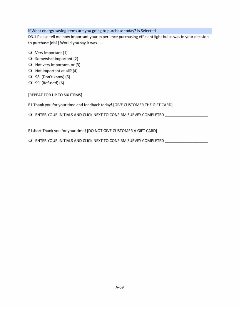
A-69
If What energy-saving items are you going to purchase today? Is Selected
D3.1 Please tell me how important your experience purchasing efficient light bulbs was in your decision
to purchase [db1] Would you say it was . . .
Very important (1)
Somewhat important (2)
Not very important, or (3)
Not important at all? (4)
98. (Don’t know) (5)
99. (Refused) (6)
[REPEAT FOR UP TO SIX ITEMS]
E1 Thank you for your time and feedback today! [GIVE CUSTOMER THE GIFT CARD]
ENTER YOUR INITIALS AND CLICK NEXT TO CONFIRM SURVEY COMPLETED ____________________
E1short Thank you for your time! [DO NOT GIVE CUSTOMER A GIFT CARD]
ENTER YOUR INITIALS AND CLICK NEXT TO CONFIRM SURVEY COMPLETED ____________________
Utah 2013‐2014 HES Evaluation Appendix B1
Appendix B. Lighting Impacts
This appendix contains further details on the following lighting topics that are introduced in the main
body of the report:
1. Hours of Use (HOU)
2. Delta Watts
3. Cross‐Sector Sales
4. Demand Elasticity Modeling
Where applicable, Cadmus followed the Uniform Methods Protocol for lighting impact evaluations.1
HOU Cadmus estimated CFL and LED HOU using a multistate modeling approach, built on light logger data
collected from two states: Missouri and Maryland. Missouri and Maryland metering data were also
employed in the previous 2011‐2012 evaluation, however, since both states continued to meter since
the prior evaluation, Cadmus used the most recent data available from these states. The metering
dataset consisted of a total of 2,274 loggers.
Cadmus chose these studies for the following reasons:
The majority of the data used in the 2011‐2012 evaluation was collected in 2010. Upstream
lighting programs feature customer engagement and educational components as well as
providing incentives for efficient lighting products. Updating data sources captures changes in
behaviors over time as a result of these components.
These extended studies also accounted for CFLs and LEDs separately, which allows Cadmus to
estimate HOU for each lighting technology. Prior metering data did not account for this
breakout as LEDs were much rarer a few years ago.
Maryland and Missouri are the most representative states as far as latitude, which is important
as daylight hours are strongly correlated with HOU.
These two studies employed a sampling strategy that prioritized rooms where efficient lighting
is most likely to be installed.
The total number of loggers was greater than the five combined studies from the previous
evaluation (2,274 compared to 2,106 in 2011‐2012). This allowed Cadmus to choose the most
representative studies without sacrificing precision with smaller numbers of loggers.
Missouri and Maryland Metering Protocol
Following whole‐house lighting audits, Cadmus installed up to 10 light meters on randomly selected
lighting fixture groups, targeting incandescents, CFLs, and medium screw‐based LEDs. To ensure
1 Available online at: http://www1.eere.energy.gov/wip/pdfs/53827‐6.pdf
Utah 2013‐2014 HES Evaluation Appendix B2
unbiased installations, Cadmus used an iPad tool to randomly select fixtures receiving the meters. The
iPad tool assigned meter installations based on room priorities, with the first five meters assigned to
each of five priority room types (e.g., living area, dining room, kitchen, master bedroom, bathroom). The
remaining five meters were randomly assigned to any fixture in any non‐priority room (e.g., secondary
bedrooms, closet, hall, basement, office, laundry, mechanical). Randomly assigning meters in this
manner sought to improve precision around priority rooms (where most lamps are installed).
Data from the removal site visits were incorporated into the iPad tool and database to augment the
installation information for each site and meter. As part of the lighting logger removal process,
technicians conducted a series of pre‐removal meter diagnostics, which included the following:
Completing a logger state test (which determined if the meter functioned properly and whether
ambient light affected the meter’s operation);
A visual review of the total time the logger recorded the fixture switched to on;
Verbal verification from the customer that they used the light fixture;
Verbal verification from the customer that the logger remained in place for the study’s
duration; and
Recording the condition of the logger and battery status.
Model Specification
To estimate HOU, Cadmus determined the total “on” time for each individual light logger per day, using
the following guidelines:
If a light logger did not record any light for an entire day, the day’s HOU was set to zero.
If a light logger registered a light turned on at 8:30 p.m. on Monday and turned off at 1:30 a.m.
on Tuesday morning, 3.5 hours were added to Monday’s HOU and 1.5 hours to Tuesday’s HOU.
Cadmus modeled daily HOU as a function of room type using an analysis of covariance (ANCOVA) model.
ANCOVA models are regression models that model a continuous variable as a function of a single,
continuous, explanatory variable and a set of binary variables. This way, an ANCOVA model simply
serves as an analysis of variance (ANOVA) model with a continuous explanatory variable added.
Cadmus chose this specification due to its simplicity, making it suitable in a wide variety of contexts.
Though the model lacked the specificity of other methods, it offered estimates not nearly as sensitive to
small differences in explanatory variables (compared to more complex methods). Therefore, these
models could produce consistent estimates of average daily HOU for a given region, using the specific
distribution of bulbs by room.
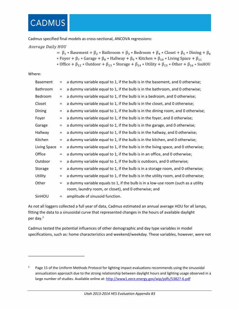
Utah 2013‐2014 HES Evaluation Appendix B3
Cadmus specified final models as cross‐sectional, ANCOVA regressions:
β ∗ Basement β ∗ Bathroom β ∗ Bedroom β ∗ Closet β ∗ Dining β
∗ Foyer β ∗ Garage β ∗ Hallway β ∗ Kitchen β ∗ LivingSpace β∗ Office β ∗ Outdoor β ∗ Storage β ∗ Utility β ∗ Other β ∗ SinHOU
Where:
Basement = a dummy variable equal to 1, if the bulb is in the basement, and 0 otherwise;
Bathroom = a dummy variable equal to 1, if the bulb is in the bathroom, and 0 otherwise;
Bedroom = a dummy variable equal to 1, if the bulb is in a bedroom, and 0 otherwise;
Closet = a dummy variable equal to 1, if the bulb is in the closet, and 0 otherwise;
Dining = a dummy variable equal to 1, if the bulb is in the dining room, and 0 otherwise;
Foyer = a dummy variable equal to 1, if the bulb is in the foyer, and 0 otherwise;
Garage = a dummy variable equal to 1, if the bulb is in the garage, and 0 otherwise;
Hallway = a dummy variable equal to 1, if the bulb is in the hallway, and 0 otherwise;
Kitchen = a dummy variable equal to 1, if the bulb is in the kitchen, and 0 otherwise;
Living Space = a dummy variable equal to 1, if the bulb is in the living space, and 0 otherwise;
Office = a dummy variable equal to 1, if the bulb is in an office, and 0 otherwise;
Outdoor = a dummy variable equal to 1, if the bulb is outdoors, and 0 otherwise;
Storage = a dummy variable equal to 1, if the bulb is in a storage room, and 0 otherwise;
Utility = a dummy variable equal to 1, if the bulb is in the utility room, and 0 otherwise;
Other = a dummy variable equals to 1, if the bulb is in a low‐use room (such as a utility
room, laundry room, or closet), and 0 otherwise; and
SinHOU = amplitude of sinusoid function.
As not all loggers collected a full year of data, Cadmus estimated an annual average HOU for all lamps,
fitting the data to a sinusoidal curve that represented changes in the hours of available daylight
per day.2
Cadmus tested the potential influences of other demographic and day type variables in model
specifications, such as: home characteristics and weekend/weekday. These variables, however, were not
2 Page 15 of the Uniform Methods Protocol for lighting impact evaluations recommends using the sinusoidal
annualization approach due to the strong relationship between daylight hours and lighting usage observed in a
large number of studies. Available online at: http://www1.eere.energy.gov/wip/pdfs/53827‐6.pdf
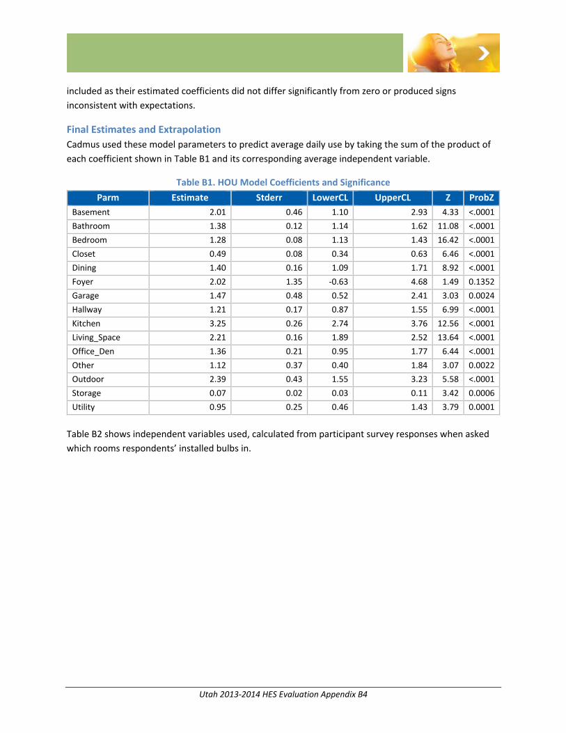
Utah 2013‐2014 HES Evaluation Appendix B4
included as their estimated coefficients did not differ significantly from zero or produced signs
inconsistent with expectations.
Final Estimates and Extrapolation
Cadmus used these model parameters to predict average daily use by taking the sum of the product of
each coefficient shown in Table B1 and its corresponding average independent variable.
Table B1. HOU Model Coefficients and Significance
Parm Estimate Stderr LowerCL UpperCL Z ProbZ
Basement 2.01 0.46 1.10 2.93 4.33 <.0001
Bathroom 1.38 0.12 1.14 1.62 11.08 <.0001
Bedroom 1.28 0.08 1.13 1.43 16.42 <.0001
Closet 0.49 0.08 0.34 0.63 6.46 <.0001
Dining 1.40 0.16 1.09 1.71 8.92 <.0001
Foyer 2.02 1.35 ‐0.63 4.68 1.49 0.1352
Garage 1.47 0.48 0.52 2.41 3.03 0.0024
Hallway 1.21 0.17 0.87 1.55 6.99 <.0001
Kitchen 3.25 0.26 2.74 3.76 12.56 <.0001
Living_Space 2.21 0.16 1.89 2.52 13.64 <.0001
Office_Den 1.36 0.21 0.95 1.77 6.44 <.0001
Other 1.12 0.37 0.40 1.84 3.07 0.0022
Outdoor 2.39 0.43 1.55 3.23 5.58 <.0001
Storage 0.07 0.02 0.03 0.11 3.42 0.0006
Utility 0.95 0.25 0.46 1.43 3.79 0.0001
Table B2 shows independent variables used, calculated from participant survey responses when asked
which rooms respondents’ installed bulbs in.
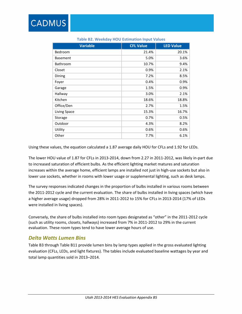
Utah 2013‐2014 HES Evaluation Appendix B5
Table B2. Weekday HOU Estimation Input Values
Variable CFL Value LED Value
Bedroom 21.4% 20.1%
Basement 5.0% 3.6%
Bathroom 10.7% 9.4%
Closet 0.9% 2.1%
Dining 7.2% 8.5%
Foyer 0.4% 0.9%
Garage 1.5% 0.9%
Hallway 3.0% 2.1%
Kitchen 18.6% 18.8%
Office/Den 2.7% 1.5%
Living Space 15.3% 16.7%
Storage 0.7% 0.5%
Outdoor 4.3% 8.2%
Utility 0.6% 0.6%
Other 7.7% 6.1%
Using these values, the equation calculated a 1.87 average daily HOU for CFLs and 1.92 for LEDs.
The lower HOU value of 1.87 for CFLs in 2013‐2014, down from 2.27 in 2011‐2012, was likely in‐part due
to increased saturation of efficient bulbs. As the efficient lighting market matures and saturation
increases within the average home, efficient lamps are installed not just in high‐use sockets but also in
lower use sockets, whether in rooms with lower usage or supplemental lighting, such as desk lamps.
The survey responses indicated changes in the proportion of bulbs installed in various rooms between
the 2011‐2012 cycle and the current evaluation. The share of bulbs installed in living spaces (which have
a higher average usage) dropped from 28% in 2011‐2012 to 15% for CFLs in 2013‐2014 (17% of LEDs
were installed in living spaces).
Conversely, the share of bulbs installed into room types designated as “other” in the 2011‐2012 cycle (such as utility rooms, closets, hallways) increased from 7% in 2011‐2012 to 29% in the current evaluation. These room types tend to have lower average hours of use.
Delta Watts Lumen Bins Table B3 through Table B11 provide lumen bins by lamp types applied in the gross evaluated lighting
evaluation (CFLs, LEDs, and light fixtures). The tables include evaluated baseline wattages by year and
total lamp quantities sold in 2013–2014.
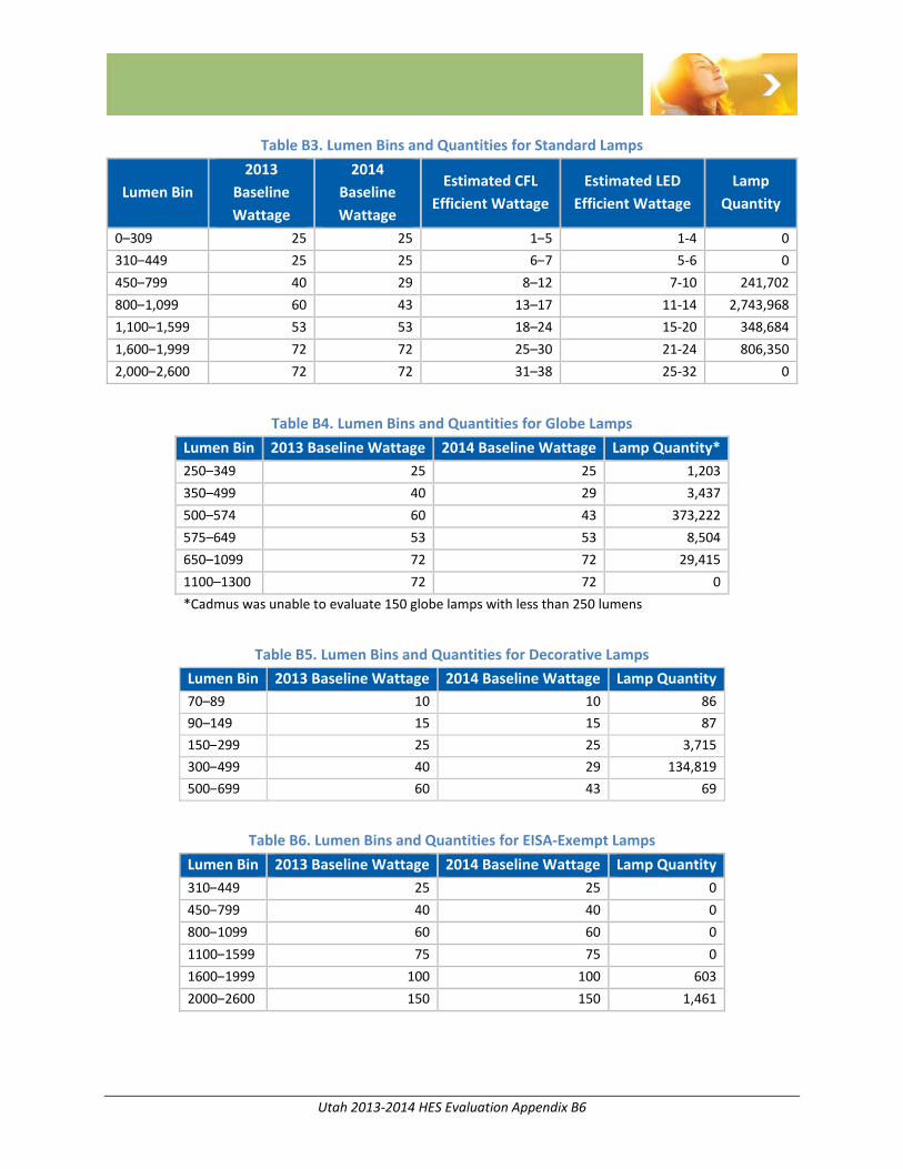
Utah 2013‐2014 HES Evaluation Appendix B6
Table B3. Lumen Bins and Quantities for Standard Lamps
Lumen Bin
2013
Baseline
Wattage
2014
Baseline
Wattage
Estimated CFL
Efficient Wattage
Estimated LED
Efficient Wattage
Lamp
Quantity
0–309 25 25 1–5 1‐4 0
310–449 25 25 6–7 5‐6 0
450–799 40 29 8–12 7‐10 241,702
800–1,099 60 43 13–17 11‐14 2,743,968
1,100–1,599 53 53 18–24 15‐20 348,684
1,600–1,999 72 72 25–30 21‐24 806,350
2,000–2,600 72 72 31–38 25‐32 0
Table B4. Lumen Bins and Quantities for Globe Lamps
Lumen Bin 2013 Baseline Wattage 2014 Baseline Wattage Lamp Quantity*
250–349 25 25 1,203
350–499 40 29 3,437
500–574 60 43 373,222
575–649 53 53 8,504
650–1099 72 72 29,415
1100–1300 72 72 0
*Cadmus was unable to evaluate 150 globe lamps with less than 250 lumens
Table B5. Lumen Bins and Quantities for Decorative Lamps
Lumen Bin 2013 Baseline Wattage 2014 Baseline Wattage Lamp Quantity
70–89 10 10 86
90–149 15 15 87
150–299 25 25 3,715
300–499 40 29 134,819
500–699 60 43 69
Table B6. Lumen Bins and Quantities for EISA‐Exempt Lamps
Lumen Bin 2013 Baseline Wattage 2014 Baseline Wattage Lamp Quantity
310–449 25 25 0
450–799 40 40 0
800–1099 60 60 0
1100–1599 75 75 0
1600–1999 100 100 603
2000–2600 150 150 1,461
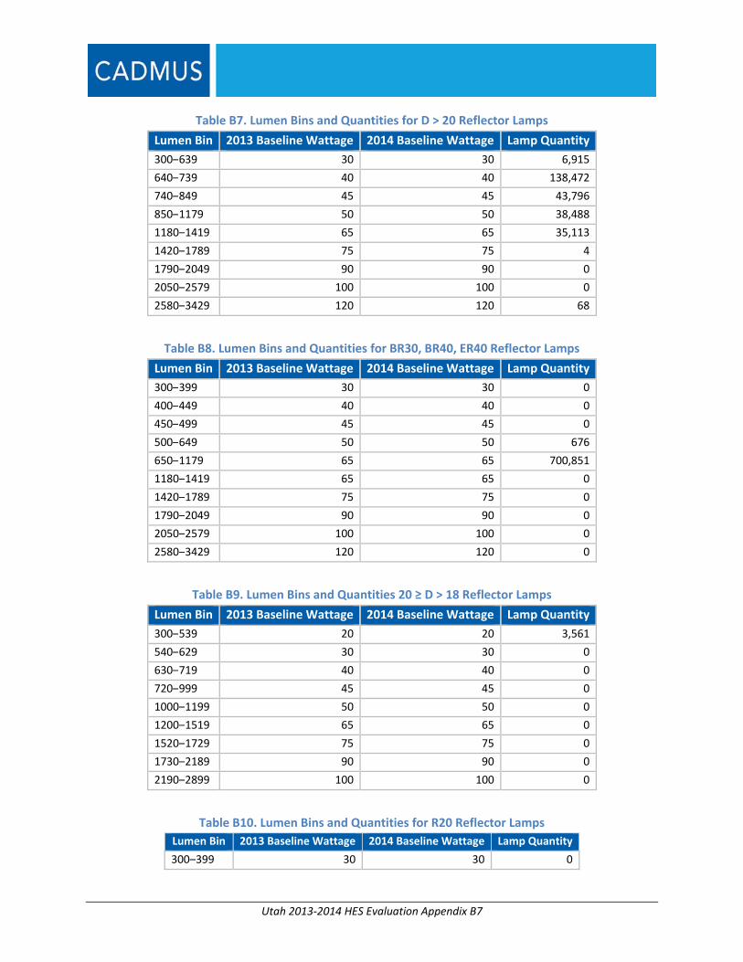
Utah 2013‐2014 HES Evaluation Appendix B7
Table B7. Lumen Bins and Quantities for D > 20 Reflector Lamps
Lumen Bin 2013 Baseline Wattage 2014 Baseline Wattage Lamp Quantity
300–639 30 30 6,915
640–739 40 40 138,472
740–849 45 45 43,796
850–1179 50 50 38,488
1180–1419 65 65 35,113
1420–1789 75 75 4
1790–2049 90 90 0
2050–2579 100 100 0
2580–3429 120 120 68
Table B8. Lumen Bins and Quantities for BR30, BR40, ER40 Reflector Lamps
Lumen Bin 2013 Baseline Wattage 2014 Baseline Wattage Lamp Quantity
300–399 30 30 0
400–449 40 40 0
450–499 45 45 0
500–649 50 50 676
650–1179 65 65 700,851
1180–1419 65 65 0
1420–1789 75 75 0
1790–2049 90 90 0
2050–2579 100 100 0
2580–3429 120 120 0
Table B9. Lumen Bins and Quantities 20 ≥ D > 18 Reflector Lamps
Lumen Bin 2013 Baseline Wattage 2014 Baseline Wattage Lamp Quantity
300–539 20 20 3,561
540–629 30 30 0
630–719 40 40 0
720–999 45 45 0
1000–1199 50 50 0
1200–1519 65 65 0
1520–1729 75 75 0
1730–2189 90 90 0
2190–2899 100 100 0
Table B10. Lumen Bins and Quantities for R20 Reflector Lamps
Lumen Bin 2013 Baseline Wattage 2014 Baseline Wattage Lamp Quantity
300–399 30 30 0

Utah 2013‐2014 HES Evaluation Appendix B8
400–449 40 40 1,410
450–719 45 45 23,218
720–999 50 50 0
1000–1199 65 65 0
1200–1519 75 75 0
1520–1729 90 90 0
1730–2189 100 100 0
2190–2899 120 120 0
Table B11. Lumen Bins and Quantities for 18 ≥ D Reflector Lamps
Lumen Bin 2013 Baseline Wattage 2014 Baseline Wattage Lamp Quantity
200‐299 20 20 0
300‐399 30 30 294
400‐449 40 40 0
450‐499 45 45 0
500‐649 50 50 0
650‐1199 65 65 0
Figure B1 displays 2014 baseline wattage plotted as a function of lumen output for standard, globe,
decorative, and EISA‐exempt lamps, as well as the three most common reflector types. This figure shows
this correlation up to 2000 lumens (only 0.03% of lamps had lumen output greater than 2000 lm).
Figure B1: Plot of 2014 Baseline Wattage vs. Lamp Lumens for Various Lamp Types
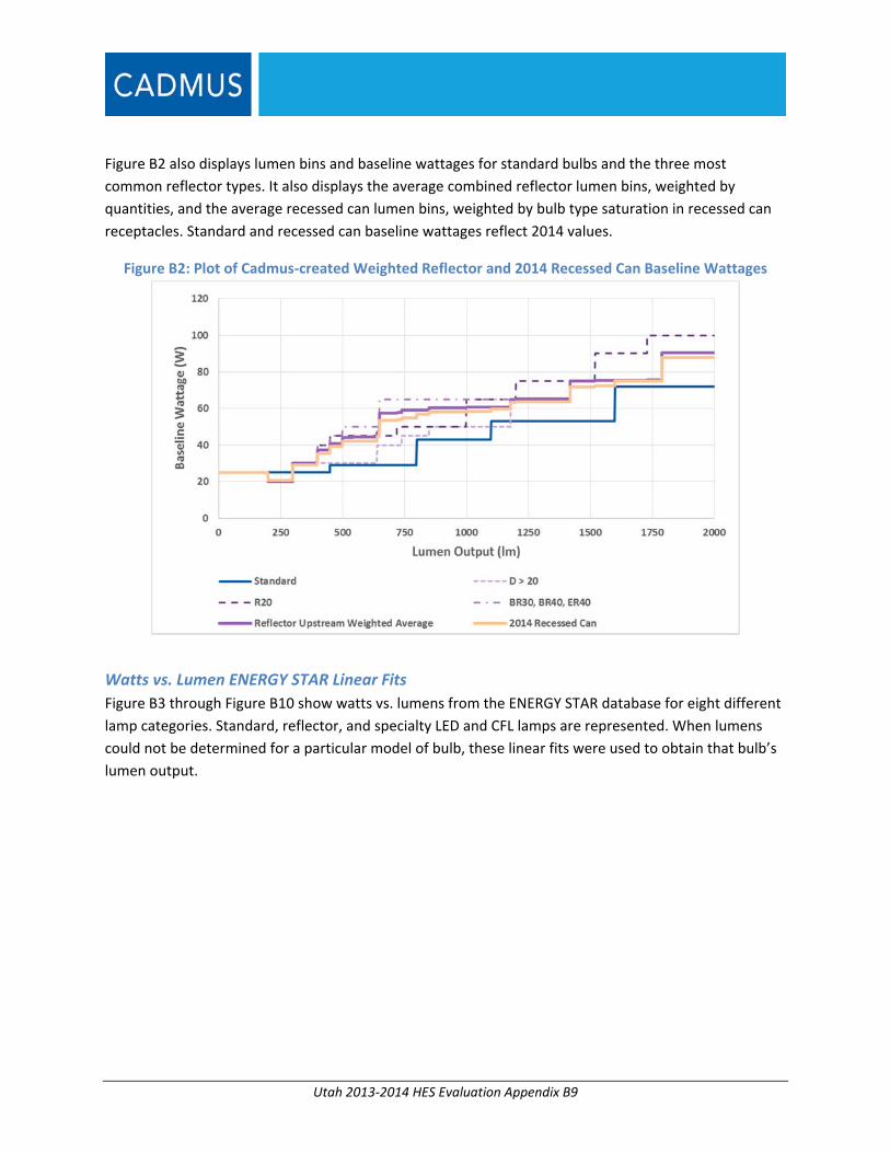
Utah 2013‐2014 HES Evaluation Appendix B9
Figure B2 also displays lumen bins and baseline wattages for standard bulbs and the three most
common reflector types. It also displays the average combined reflector lumen bins, weighted by
quantities, and the average recessed can lumen bins, weighted by bulb type saturation in recessed can
receptacles. Standard and recessed can baseline wattages reflect 2014 values.
Figure B2: Plot of Cadmus‐created Weighted Reflector and 2014 Recessed Can Baseline Wattages
Watts vs. Lumen ENERGY STAR Linear Fits
Figure B3 through Figure B10 show watts vs. lumens from the ENERGY STAR database for eight different
lamp categories. Standard, reflector, and specialty LED and CFL lamps are represented. When lumens
could not be determined for a particular model of bulb, these linear fits were used to obtain that bulb’s
lumen output.

Utah 2013‐2014 HES Evaluation Appendix B10
Figure B3: Median Lumens vs. Wattage for ENERGY STAR‐Qualified Standard CFLs
Figure B4: Median Lumens vs. Wattage for ENERGY STAR‐Qualified Reflector CFLs
Figure B5: Median Lumens vs. Wattage for ENERGY STAR‐Qualified Specialty CFLs
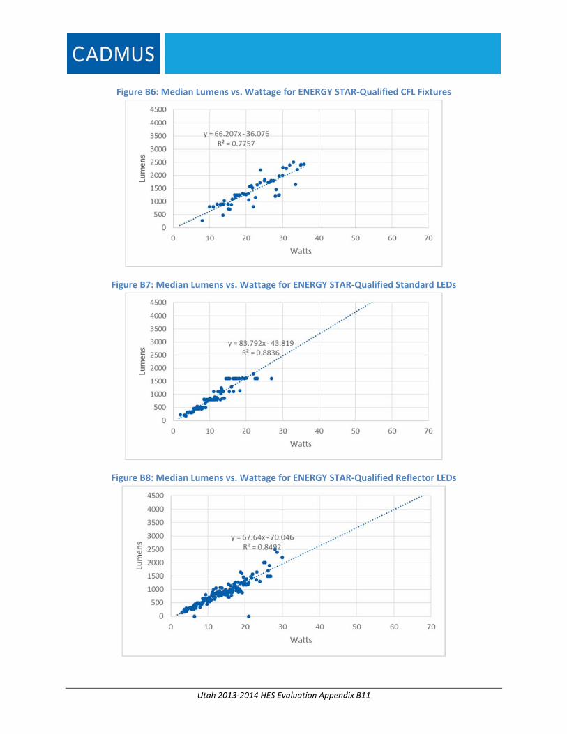
Utah 2013‐2014 HES Evaluation Appendix B11
Figure B6: Median Lumens vs. Wattage for ENERGY STAR‐Qualified CFL Fixtures
Figure B7: Median Lumens vs. Wattage for ENERGY STAR‐Qualified Standard LEDs
Figure B8: Median Lumens vs. Wattage for ENERGY STAR‐Qualified Reflector LEDs
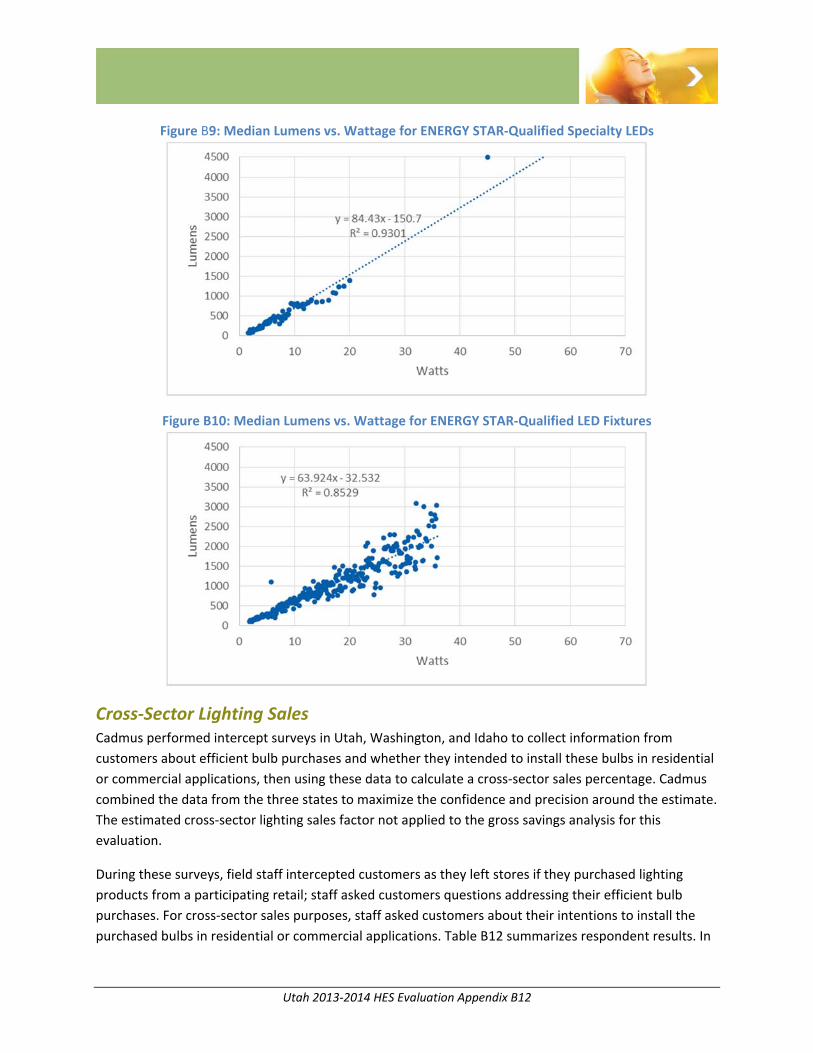
Utah 2013‐2014 HES Evaluation Appendix B12
Figure B9: Median Lumens vs. Wattage for ENERGY STAR‐Qualified Specialty LEDs
Figure B10: Median Lumens vs. Wattage for ENERGY STAR‐Qualified LED Fixtures
Cross‐Sector Lighting Sales Cadmus performed intercept surveys in Utah, Washington, and Idaho to collect information from
customers about efficient bulb purchases and whether they intended to install these bulbs in residential
or commercial applications, then using these data to calculate a cross‐sector sales percentage. Cadmus
combined the data from the three states to maximize the confidence and precision around the estimate.
The estimated cross‐sector lighting sales factor not applied to the gross savings analysis for this
evaluation.
During these surveys, field staff intercepted customers as they left stores if they purchased lighting
products from a participating retail; staff asked customers questions addressing their efficient bulb
purchases. For cross‐sector sales purposes, staff asked customers about their intentions to install the
purchased bulbs in residential or commercial applications. Table B12 summarizes respondent results. In
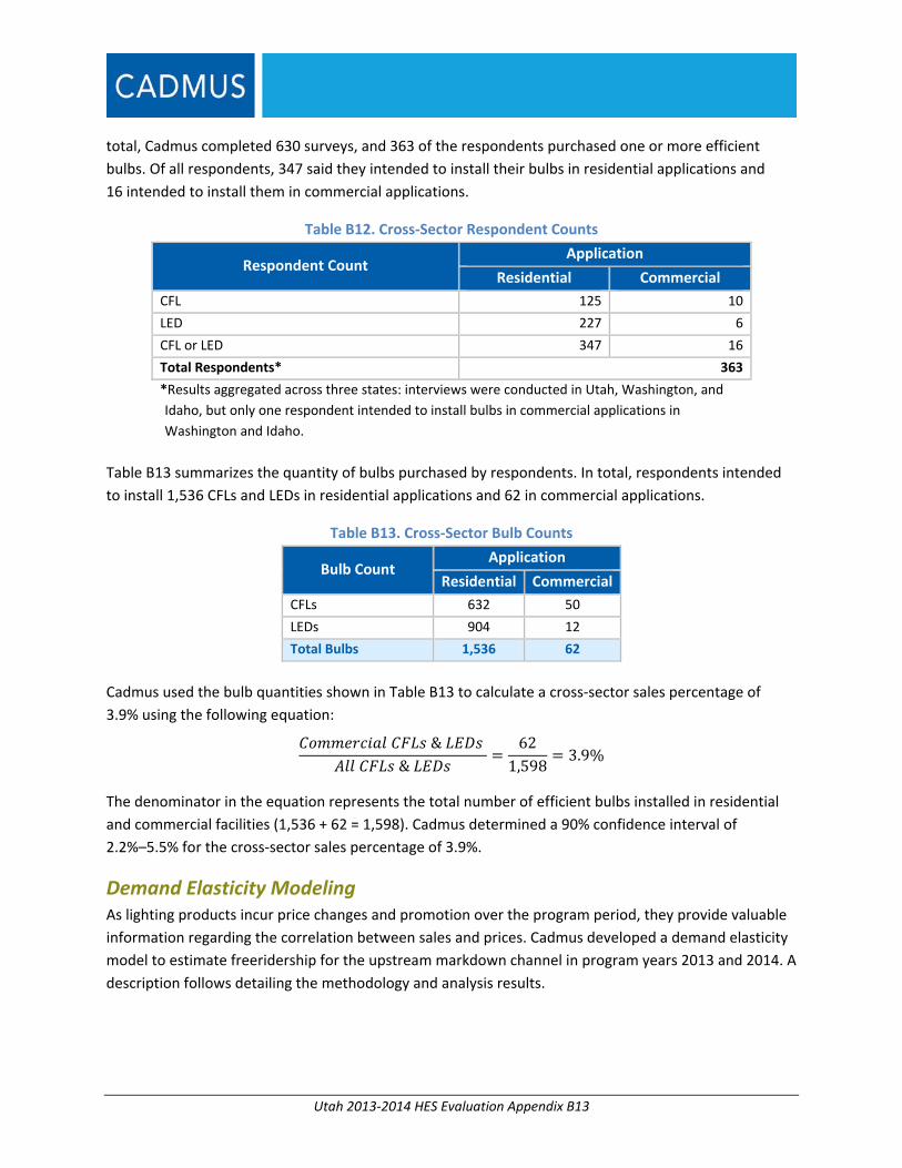
Utah 2013‐2014 HES Evaluation Appendix B13
total, Cadmus completed 630 surveys, and 363 of the respondents purchased one or more efficient
bulbs. Of all respondents, 347 said they intended to install their bulbs in residential applications and
16 intended to install them in commercial applications.
Table B12. Cross‐Sector Respondent Counts
Respondent Count Application
Residential Commercial
CFL 125 10
LED 227 6
CFL or LED 347 16
Total Respondents* 363
*Results aggregated across three states: interviews were conducted in Utah, Washington, and
Idaho, but only one respondent intended to install bulbs in commercial applications in
Washington and Idaho.
Table B13 summarizes the quantity of bulbs purchased by respondents. In total, respondents intended
to install 1,536 CFLs and LEDs in residential applications and 62 in commercial applications.
Table B13. Cross‐Sector Bulb Counts
Bulb Count Application
Residential Commercial
CFLs 632 50
LEDs 904 12
Total Bulbs 1,536 62
Cadmus used the bulb quantities shown in Table B13 to calculate a cross‐sector sales percentage of
3.9% using the following equation:
& &
621,598
3.9%
The denominator in the equation represents the total number of efficient bulbs installed in residential
and commercial facilities (1,536 + 62 = 1,598). Cadmus determined a 90% confidence interval of
2.2%–5.5% for the cross‐sector sales percentage of 3.9%.
Demand Elasticity Modeling As lighting products incur price changes and promotion over the program period, they provide valuable
information regarding the correlation between sales and prices. Cadmus developed a demand elasticity
model to estimate freeridership for the upstream markdown channel in program years 2013 and 2014. A
description follows detailing the methodology and analysis results.

Utah 2013‐2014 HES Evaluation Appendix B14
Demand Elasticity Methodology
Demand elasticity modeling draws upon the same economic principle that drives program design:
changes in price and promotion generate changes in quantities sold (i.e., the upstream buy‐down
approach). Demand elasticity modeling uses sales and promotion information to achieve the following:
Quantify the relationship of price and promotion to sales;
Determine likely sales levels without the program’s intervention (baseline sales); and
Estimate freeridership by comparing modeled baseline sales with actual sales.
After estimating variable coefficients, Cadmus used the resulting model to predict the following:
Sales that would occur without the program’s price impact; and
Sales that would occur with the program (and should be close to actual sales with a
representative model).
Once the model predicted sales that would occur with and without the program, Cadmus applied
evaluated savings values, calculated as part of this evaluation.
Cadmus then calculated savings net of freeridership3 using the following formula:
Input Data
As the demand elasticity approach relies exclusively on program data, a model’s robustness depends on
data quality. Though, overall, available data achieved a sufficient quality to support the analysis, the
data also presented several issues of note:
1. Inconsistent model numbers between 2013 and 2014.
2. Lack of schedule ID number in 2013 data.
3. Inconsistent bulb type designations within each model number (e.g., spiral and candelabra,
reflector and general purpose spiral/a‐line).
4. Inconsistent reported quantities within a given sales period.
Cadmus had to make the most reasonable assumptions possible when preparing the data to support the
analysis (e.g., assessing whether two model numbers with different formats and detail levels were
the same).
3 Net of FR are sales net of freeridership, or 1‐FR, used to calculate the net‐to‐gross (NTG) ratio where NTG = 1 –
FR + Spillover. For this evaluation, spillover was assumed to be 0%.

Utah 2013‐2014 HES Evaluation Appendix B15
Price Variation
As desired for analysis, sales data displayed relatively high amounts of price variations. Variation was
measured within unique part number/retailer location combinations: that is, a given bulb model within
a unique retail location.
Promotional Displays
The program administrator, did not collect and could not provide detailed data on product
merchandising (e.g., clip strips, end caps, pallet displays). Therefore, the model may not have captured
all program impacts.4
Evaluations in other jurisdictions have found that product merchandising can generate sales lift between
60% and 120%. Capturing and providing this level of detail ensures that the program is credited for
all activities.
Stocking Patterns
In preparing to model the sales data, Cadmus observed dramatic sales drops that did not correspond to
programmatic activity or to expected seasonal variation. Cadmus’ model implicitly assumed supply
would meet demand at the given price. Analysis included screening the data for instances where this
assumption appeared untrue.
Cadmus looked for patterns in these drops that suggested changes in stocking patterns or retailers
temporarily unable to stock certain products. The following criteria served to flag changes in
stocking patterns:
1. Average monthly sales for a product were greater than 10 packs. For those fewer than 10
packs per month, Cadmus assumed it would be more likely that some months would have zero
sales.5
2. Two‐thirds of monthly observations of the same product across multiple store locations
proved less than one pack.6 For example, if a 13‐watt GE spiral CFL was sold at 18 different
store locations, and 14 locations had sales of less than one pack during the month of June.
4 To the degree that product merchandising and prices co‐vary, elasticity estimates may capture some sales lift
generated by merchandising. However, as data were not available to incorporate into the model, it impossible
to estimate separate impacts.
5 The 10 packs cutoff assumed that products with average monthly sales fewer than 10 would be more likely to
have months with zero sales due to naturally occurring variability. 6 Because the sales data are reported at intervals that do not follow regular calendar months, the sales are
transformed to daily sales and then aggregated by calendar month. This leads to fractional package sales within a given month though overall quantities remain the same.
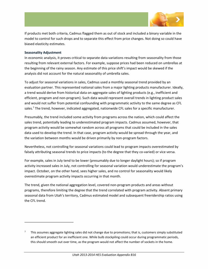
Utah 2013‐2014 HES Evaluation Appendix B16
If products met both criteria, Cadmus flagged them as out of stock and included a binary variable in the
model to control for such drops and to separate this effect from price changes. Not doing so could have
biased elasticity estimates.
Seasonality Adjustment
In economic analysis, it proves critical to separate data variations resulting from seasonality from those
resulting from relevant external factors. For example, suppose prices had been reduced on umbrellas at
the beginning of the rainy season. Any estimate of this price shift’s impact would be skewed if the
analysis did not account for the natural seasonality of umbrella sales.
To adjust for seasonal variations in sales, Cadmus used a monthly seasonal trend provided by an
evaluation partner. This represented national sales from a major lighting products manufacturer. Ideally,
a trend would derive from historical data on aggregate sales of lighting products (e.g., inefficient and
efficient, program and non‐program). Such data would represent overall trends in lighting product sales
and would not suffer from potential confounding with programmatic activity to the same degree as CFL
sales.7 The trend, however, indicated aggregated, nationwide CFL sales for a specific manufacturer.
Presumably, the trend included some activity from programs across the nation, which could affect the
sales trend, potentially leading to underestimated program impacts. Cadmus assumed, however, that
program activity would be somewhat random across all programs that could be included in the sales
data used to develop the trend. In that case, program activity would be spread through the year, and
the variation between months would be driven primarily by non‐program factors.
Nevertheless, not controlling for seasonal variations could lead to program impacts overestimated by
falsely attributing seasonal trends to price impacts (to the degree that they co‐varied) or vice versa.
For example, sales in July tend to be lower (presumably due to longer daylight hours); so if program
activity increased sales in July, not controlling for seasonal variation would underestimate the program’s
impact. October, on the other hand, sees higher sales, and no control for seasonality would likely
overestimate program activity impacts occurring in that month.
The trend, given the national aggregation level, covered non‐program products and areas without
programs, therefore limiting the degree that the trend correlated with program activity. Absent primary
seasonal data from Utah’s territory, Cadmus estimated model and subsequent freeridership ratios using
the CFL trend.
7 This assumes aggregate lighting sales did not change due to promotions; that is, customers simply substituted
an efficient product for an inefficient one. While bulb stockpiling could occur during programmatic periods,
this should smooth out over time, as the program would not affect the number of sockets in the home.

Utah 2013‐2014 HES Evaluation Appendix B17
Model Specification
Cadmus modeled bulb, pricing, and promotional data using an econometric model, addressing these
data as a panel, with a cross‐section of program package quantities modeled over time as a function of
prices, promotional events, and retail channels. This involved testing a variety of specifications to
ascertain price impacts—the main instrument affected by the program—on bulb demand. Cadmus
estimated the following equation for the model (for bulb model i, in month t):
ln ,
∗ , ∗ ,
∗ , ,
Where: ln = Natural log
Q = Quantity of bulb packs sold during the month
P = Retail price (after markdown) in that month
Retail Channel = Retail category (Club or non‐Club store)
Bulb Type = Product category (CFL or LED)
Specialty = Dummy variable equaling 1 for specialty bulbs and 0 for standard
Out of Stock = Dummy variable equaling 1 if a given product was assumed to have been out of
stock in month t and 0 otherwise
ID = Dummy variable equaling 1 for each unique retail channel and SKU; 0 otherwise
Seasonal Trend = Quantitative trend representing the impact of secular trends not related to the
program8
= Cross‐sectional random‐error term
The model specification assumed a negative binomial distribution, which served as the best fit of the
plausible distributions (e.g., lognormal, poisson, negative binomial, gamma). The negative binomial
distribution provided accurate predictions for a small number of high‐volume sale bulbs, while the other
distributions under predicted sales for those bulbs.
Cadmus adjusted the model to correct for the two factors discussed earlier:
Seasonality: To account for baseline lighting sales tending to follow a seasonal pattern,
unrelated to price or promotion, by inserting a seasonal trend into the model.
8 The time trend for this analysis represented shifts in sales due to non‐program‐related seasonality.

Utah 2013‐2014 HES Evaluation Appendix B18
Stocking Patterns: The model assumed supply would always meet demand; after investigating
situations where this did not occur, Cadmus controlled for instances where two‐thirds or more
of monthly observations for the same product with less than one package within a given month.
Using the following criteria, Cadmus ran numerous model scenarios to identify the one with the best
parsimony and explanatory power:
Model coefficient p‐values (keeping values less than <0.1);9
Explanatory variable cross‐correlation (minimizing where possible);
Model Akaike’s Information Criteria (AIC) (minimizing between models);10
Minimizing multicollinearity; and
Optimizing model fit.
The model’s fit can be examined by comparing model‐predicted sales with actual sales. As shown in
Figure B11, the model‐predicted sales matches very closely with actual sales. The model under predicted
a couple of months, but it also over predicted a couple of months without persistent bias in a single
direction (over‐ or under‐predicting), indicating the model fit the data well. Overall, the model fell within
0.4% of actual sales.
Figure B11. Predicted and Actual Sales
9 Where a qualitative variable had many states (such as bulb types), Cadmus did not omit variables if one state’s
was insignificant; rather, the analysis considered the joint significance of all states.
10 The Team used AIC to assess model fit, as nonlinear models do not define the R‐square statistic. AIC also offers
a desirable property in that it penalizes overly complex models, similarly to the adjusted R‐square.
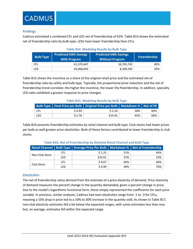
Utah 2013‐2014 HES Evaluation Appendix B19
Findings
Cadmus estimated a combined CFL and LED net of freeridership of 62%. Table B14 shows the estimated
net of freeridership ratio by bulb type. LEDs have lower freeridership than CFLs.
Table B14. Modeling Results by Bulb Type
Bulb Type Predicted kWh Savings
With Program
Predicted kWh Savings
Without Program Freeridership
CFL 41,370,447 16,765,742 40%
LED 24,468,043 8,349,595 34%
Table B15 shows the incentive as a share of the original retail price and the estimated net of
freeridership ratio by utility and bulb type. Typically, the proportional price reduction and the net of
freeridership trend correlate: the higher the incentive, the lower the freeridership. In addition, specialty
LED sales exhibited a greater response to price changes.
Table B15. Modeling Results by Bulb Type
Bulb Type Final Price per Bulb Original Price per Bulb Markdown % Net of FR
CFL $ 0.94 $ 2.24 58% 60%
LED $ 5.70 $10.45 45% 66%
Table B16 presents freeridership estimates by retail channel and bulb type. Club stores had lower prices
per bulb as well greater price elasticities. Both of these factors contributed to lower freeridership in club
stores.
Table B16. Net of Freeridership by Detailed Retail Channel and Bulb Type
Retail Channel Bulb Type Average Price Per Bulb Markdown % Net of Freeridership
Non‐Club Store CFL $ 1.25 51% 44%
LED $10.61 31% 23%
Club Store CFL $ 0.67 66% 66%
LED $ 4.99 49% 70%
Elasticities
The net of freeridership ratios derived from the estimate of a price elasticity of demand. Price elasticity
of demand measures the percent change in the quantity demanded, given a percent change in price.
Due to the model’s logarithmic functional form, these simply represented the coefficients for each price
variable. In previous, similar analyses, Cadmus had seen elasticities range from ‐1 to ‐3 for CFLs,
meaning a 10% drop in price led to a 10% to 30% increase in the quantity sold. As shown in Table B17,
non‐club elasticity estimates fell a bit below the expected ranges, with some estimates less than one,
but, on average, estimates fell within the expected range.
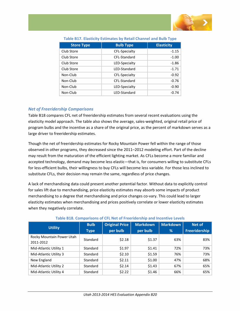
Utah 2013‐2014 HES Evaluation Appendix B20
Table B17. Elasticity Estimates by Retail Channel and Bulb Type
Store Type Bulb Type Elasticity
Club Store CFL‐Specialty ‐1.15
Club Store CFL‐Standard ‐1.00
Club Store LED‐Specialty ‐1.86
Club Store LED‐Standard ‐1.71
Non‐Club CFL‐Specialty ‐0.92
Non‐Club CFL‐Standard ‐0.76
Non‐Club LED‐Specialty ‐0.90
Non‐Club LED‐Standard ‐0.74
Net of Freeridership Comparisons
Table B18 compares CFL net of freeridership estimates from several recent evaluations using the
elasticity model approach. The table also shows the average, sales‐weighted, original retail price of
program bulbs and the incentive as a share of the original price, as the percent of markdown serves as a
large driver to freeridership estimates.
Though the net of freeridership estimates for Rocky Mountain Power fell within the range of those
observed in other programs, they decreased since the 2011–2012 modeling effort. Part of the decline
may result from the maturation of the efficient lighting market. As CFLs become a more familiar and
accepted technology, demand may become less elastic—that is, for consumers willing to substitute CFLs
for less‐efficient bulbs, their willingness to buy CFLs will become less variable. For those less inclined to
substitute CFLs, their decision may remain the same, regardless of price changes.
A lack of merchandising data could present another potential factor. Without data to explicitly control
for sales lift due to merchandising, price elasticity estimates may absorb some impacts of product
merchandising to a degree that merchandising and price changes co‐vary. This could lead to larger
elasticity estimates when merchandising and prices positively correlate or lower elasticity estimates
when they negatively correlate.
Table B18. Comparisons of CFL Net of Freeridership and Incentive Levels
Utility Bulb
Type
Original Price
per bulb
Markdown
per bulb
Markdown
%
Net of
Freeridership
Rocky Mountain Power Utah
2011‐2012 Standard $2.18 $1.37 63% 83%
Mid‐Atlantic Utility 1 Standard $1.97 $1.41 72% 73%
Mid‐Atlantic Utility 3 Standard $2.10 $1.59 76% 73%
New England Standard $2.11 $1.00 47% 68%
Mid‐Atlantic Utility 2 Standard $2.14 $1.43 67% 65%
Mid‐Atlantic Utility 4 Standard $2.22 $1.46 66% 65%
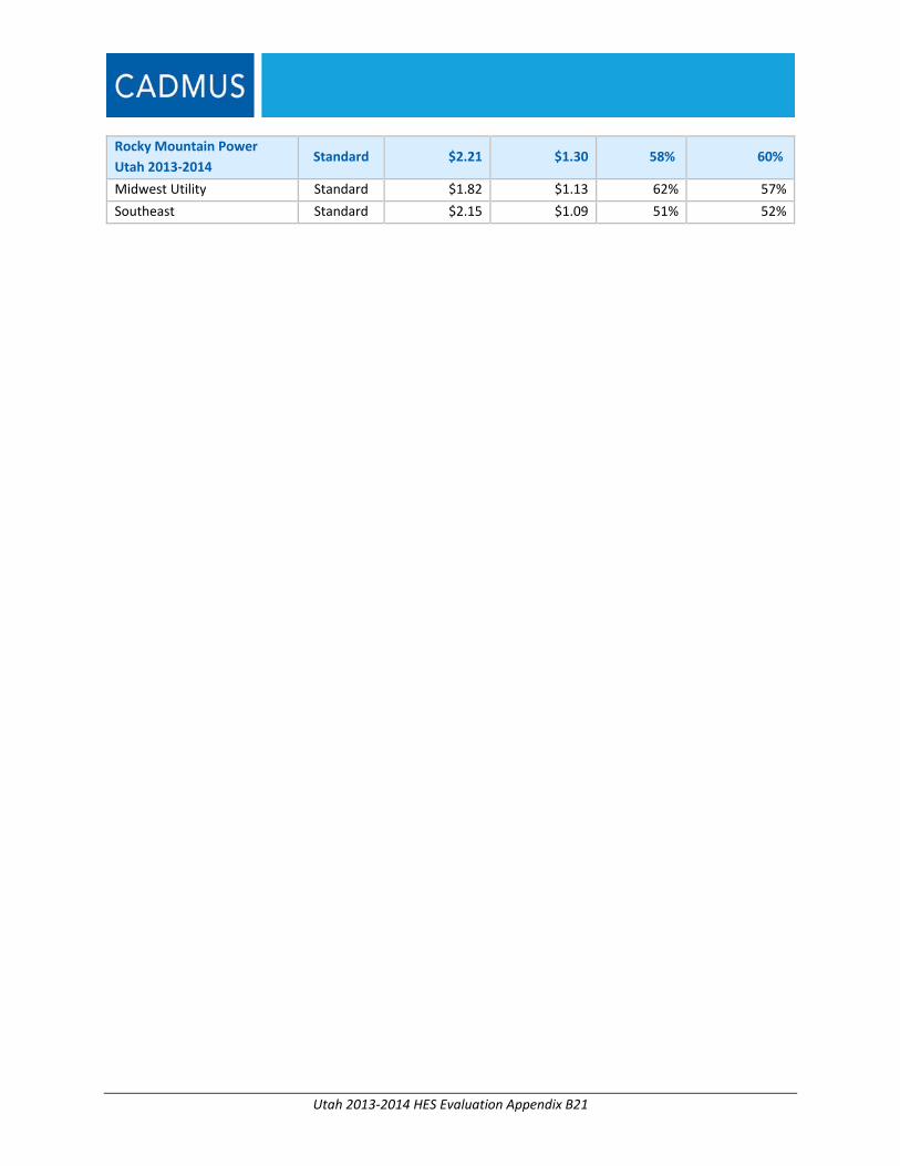
Utah 2013‐2014 HES Evaluation Appendix B21
Rocky Mountain Power
Utah 2013‐2014 Standard $2.21 $1.30 58% 60%
Midwest Utility Standard $1.82 $1.13 62% 57%
Southeast Standard $2.15 $1.09 51% 52%

Utah 2013‐2014 HES Evaluation Appendix C1
Appendix C. HES Billing Analysis
Cadmus conducted three billing analyses to estimate gross and net savings for the following measures:
Insulation (attic, wall, or floor)
Ductwork (duct sealing and/or duct insulation)
Cooling Equipment (central air conditioners and evaporative coolers)
The following sections outline the methodology and results for each effort.
Insulation Billing Analysis Cadmus conducted billing analysis to assess actual net energy savings associated with insulation
measure installations.1 Cadmus determined the savings estimate using a pooled, conditional savings
analysis (CSA) regression model, which included the following groups:
2013–2014 insulation participants (combined attic, wall, and floor insulation); and
Nonparticipant homes, serving as the comparison group.
The billing analysis resulted in a 105% net realization rate for insulation measures (a net result rather
than gross as it compares participant usage trends to a nonparticipant group, accounting for market
conditions outside of the program).
Insulation Program Data and Billing Analysis Methodology
Cadmus used the following sources to create the final database for conducting the billing analysis:
Participant program data, collected and provided by the program administrator (including
account numbers, measure types, installation dates, square footage of insulation installed, heat
sources, and expected savings for the entire participant population).
Control group data, which Cadmus collected from a census of nearly 500,000 nonparticipating
customers in Utah. Cadmus matched energy use for the control group to quartiles of the
participants’ pre‐participation energy use to ensure comparability of the two groups. To ensure
adequate coverage of the nonparticipating population, Cadmus included four times the number
of nonparticipants than participants.
Billing data, provided by Rocky Mountain Power, which included all Utah residential accounts.
Cadmus matched the 2013–2014 participant program data to the census of Utah’s billing data
for participants installing only insulation measures (i.e. did not install other measures through
HES). Billing data included meter‐read dates and kWh consumption from January 2012 through
August 2015. The final sample used in the billing analysis consisted of 6,928 participants and
27,712 control customers.
1 Billing analysis performed for customers installing only attic, wall, or floor insulation measures.
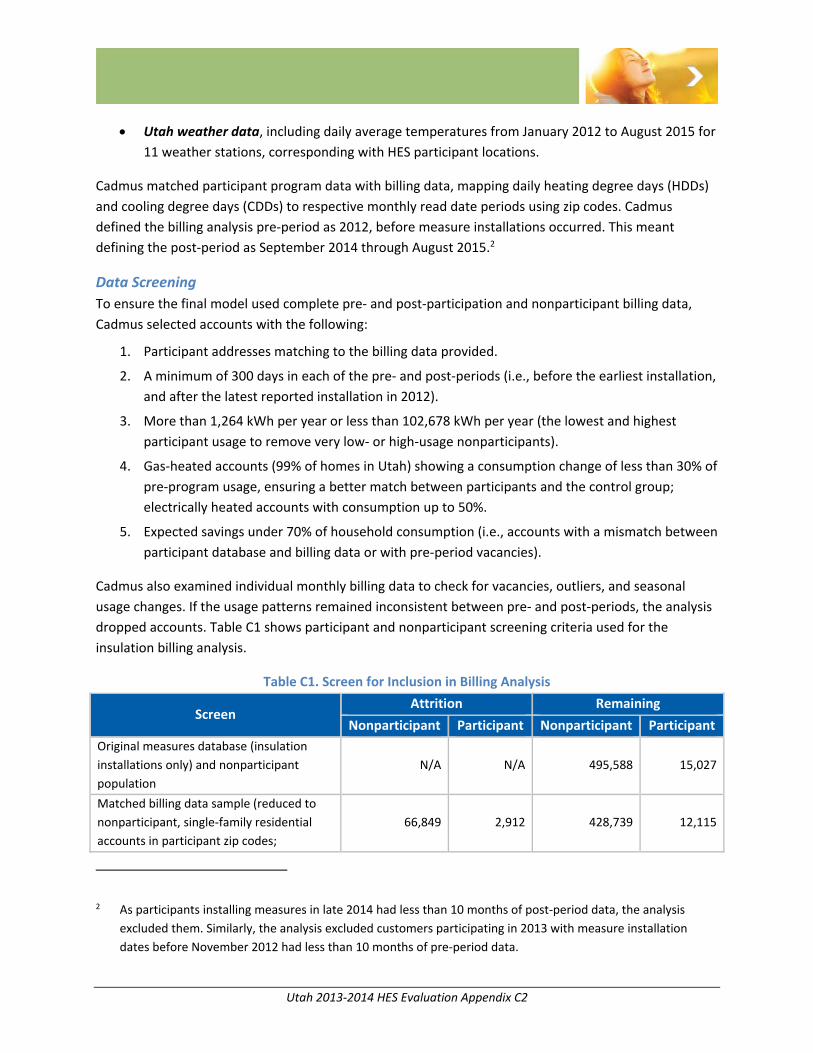
Utah 2013‐2014 HES Evaluation Appendix C2
Utah weather data, including daily average temperatures from January 2012 to August 2015 for
11 weather stations, corresponding with HES participant locations.
Cadmus matched participant program data with billing data, mapping daily heating degree days (HDDs)
and cooling degree days (CDDs) to respective monthly read date periods using zip codes. Cadmus
defined the billing analysis pre‐period as 2012, before measure installations occurred. This meant
defining the post‐period as September 2014 through August 2015.2
Data Screening
To ensure the final model used complete pre‐ and post‐participation and nonparticipant billing data,
Cadmus selected accounts with the following:
1. Participant addresses matching to the billing data provided.
2. A minimum of 300 days in each of the pre‐ and post‐periods (i.e., before the earliest installation,
and after the latest reported installation in 2012).
3. More than 1,264 kWh per year or less than 102,678 kWh per year (the lowest and highest
participant usage to remove very low‐ or high‐usage nonparticipants).
4. Gas‐heated accounts (99% of homes in Utah) showing a consumption change of less than 30% of
pre‐program usage, ensuring a better match between participants and the control group;
electrically heated accounts with consumption up to 50%.
5. Expected savings under 70% of household consumption (i.e., accounts with a mismatch between
participant database and billing data or with pre‐period vacancies).
Cadmus also examined individual monthly billing data to check for vacancies, outliers, and seasonal
usage changes. If the usage patterns remained inconsistent between pre‐ and post‐periods, the analysis
dropped accounts. Table C1 shows participant and nonparticipant screening criteria used for the
insulation billing analysis.
Table C1. Screen for Inclusion in Billing Analysis
Screen Attrition Remaining
Nonparticipant Participant Nonparticipant Participant
Original measures database (insulation
installations only) and nonparticipant
population
N/A N/A 495,588 15,027
Matched billing data sample (reduced to
nonparticipant, single‐family residential
accounts in participant zip codes;
66,849 2,912 428,739 12,115
2 As participants installing measures in late 2014 had less than 10 months of post‐period data, the analysis
excluded them. Similarly, the analysis excluded customers participating in 2013 with measure installation
dates before November 2012 had less than 10 months of pre‐period data.
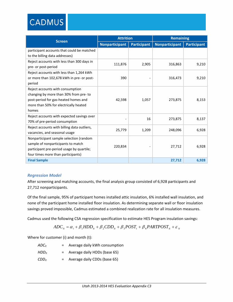
Utah 2013‐2014 HES Evaluation Appendix C3
Screen Attrition Remaining
Nonparticipant Participant Nonparticipant Participant
participant accounts that could be matched
to the billing data addresses)
Reject accounts with less than 300 days in
pre‐ or post‐period 111,876 2,905 316,863 9,210
Reject accounts with less than 1,264 kWh
or more than 102,678 kWh in pre‐ or post‐
period
390 ‐ 316,473 9,210
Reject accounts with consumption
changing by more than 30% from pre‐ to
post‐period for gas‐heated homes and
more than 50% for electrically heated
homes
42,598 1,057 273,875 8,153
Reject accounts with expected savings over
70% of pre‐period consumption ‐ 16 273,875 8,137
Reject accounts with billing data outliers,
vacancies, and seasonal usage 25,779 1,209 248,096 6,928
Nonparticipant sample selection (random
sample of nonparticipants to match
participant pre‐period usage by quartile;
four times more than participants)
220,834 ‐ 27,712 6,928
Final Sample 27,712 6,928
Regression Model
After screening and matching accounts, the final analysis group consisted of 6,928 participants and
27,712 nonparticipants.
Of the final sample, 95% of participant homes installed attic insulation, 6% installed wall insulation, and
none of the participant home installed floor insulation. As determining separate wall or floor insulation
savings proved impossible, Cadmus estimated a combined realization rate for all insulation measures.
Cadmus used the following CSA regression specification to estimate HES Program insulation savings:
itittititiit PARTPOSTPOSTCDDHDDADC 4321
Where for customer (i) and month (t):
ADCit = Average daily kWh consumption
HDDit = Average daily HDDs (base 65)
CDDit = Average daily CDDs (base 65)
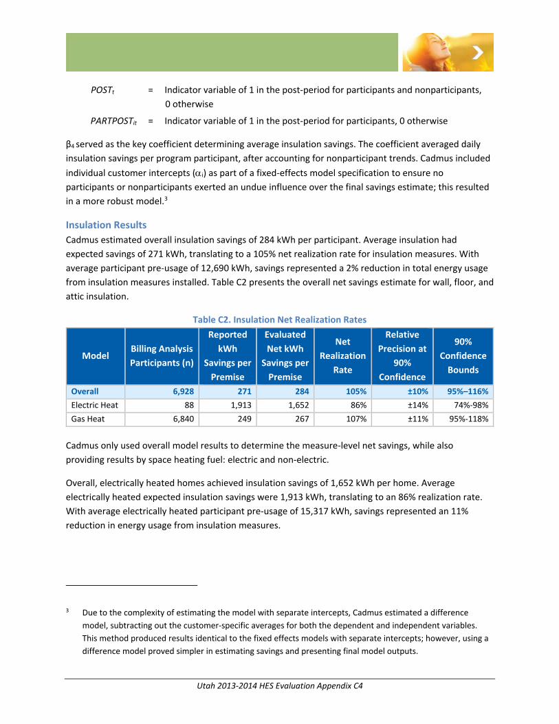
Utah 2013‐2014 HES Evaluation Appendix C4
POSTt = Indicator variable of 1 in the post‐period for participants and nonparticipants,
0 otherwise
PARTPOSTit = Indicator variable of 1 in the post‐period for participants, 0 otherwise
β4 served as the key coefficient determining average insulation savings. The coefficient averaged daily
insulation savings per program participant, after accounting for nonparticipant trends. Cadmus included
individual customer intercepts (i) as part of a fixed‐effects model specification to ensure no
participants or nonparticipants exerted an undue influence over the final savings estimate; this resulted
in a more robust model.3
Insulation Results
Cadmus estimated overall insulation savings of 284 kWh per participant. Average insulation had
expected savings of 271 kWh, translating to a 105% net realization rate for insulation measures. With
average participant pre‐usage of 12,690 kWh, savings represented a 2% reduction in total energy usage
from insulation measures installed. Table C2 presents the overall net savings estimate for wall, floor, and
attic insulation.
Table C2. Insulation Net Realization Rates
Model Billing Analysis
Participants (n)
Reported
kWh
Savings per
Premise
Evaluated
Net kWh
Savings per
Premise
Net
Realization
Rate
Relative
Precision at
90%
Confidence
90%
Confidence
Bounds
Overall 6,928 271 284 105% ±10% 95%–116%
Electric Heat 88 1,913 1,652 86% ±14% 74%‐98%
Gas Heat 6,840 249 267 107% ±11% 95%‐118%
Cadmus only used overall model results to determine the measure‐level net savings, while also
providing results by space heating fuel: electric and non‐electric.
Overall, electrically heated homes achieved insulation savings of 1,652 kWh per home. Average
electrically heated expected insulation savings were 1,913 kWh, translating to an 86% realization rate.
With average electrically heated participant pre‐usage of 15,317 kWh, savings represented an 11%
reduction in energy usage from insulation measures.
3 Due to the complexity of estimating the model with separate intercepts, Cadmus estimated a difference
model, subtracting out the customer‐specific averages for both the dependent and independent variables.
This method produced results identical to the fixed effects models with separate intercepts; however, using a
difference model proved simpler in estimating savings and presenting final model outputs.
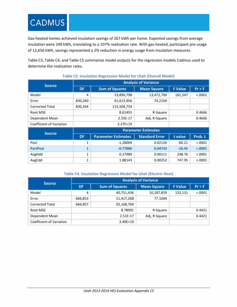
Utah 2013‐2014 HES Evaluation Appendix C5
Gas‐heated homes achieved insulation savings of 267 kWh per home. Expected savings from average
insulation were 249 kWh, translating to a 107% realization rate. With gas‐heated, participant pre‐usage
of 12,656 kWh, savings represented a 2% reduction in energy usage from insulation measures.
Table C3, Table C4, and Table C5 summarize model outputs for the regression models Cadmus used to
determine the realization rates.
Table C3. Insulation Regression Model for Utah (Overall Model)
Source Analysis of Variance
DF Sum of Squares Mean Square F Value Pr > F
Model 4 53,890,798 13,472,700 181,547 <.0001
Error 830,260 61,613,956 74.2104
Corrected Total 830,264 115,504,754
Root MSE 8.61455 R‐Square 0.4666
Dependent Mean 2.55E‐17 Adj. R‐Square 0.4666
Coefficient of Variation 3.37E+19
Source Parameter Estimates
DF Parameter Estimates Standard Error t value Prob. t
Post 1 ‐1.28009 0.02126 ‐60.21 <.0001
PartPost 1 ‐0.77886 0.04733 ‐16.45 <.0001
AvgHdd 1 0.27489 0.00111 248.76 <.0001
AvgCdd 1 1.88143 0.00252 747.95 <.0001
Table C4. Insulation Regression Model for Utah (Electric Heat)
Source Analysis of Variance
DF Sum of Squares Mean Square F Value Pr > F
Model 4 40,751,436 10,187,859 132,131 <.0001
Error 666,853 51,417,268 77.1044
Corrected Total 666,857 92,168,704
Root MSE 8.78091 R‐Square 0.4421
Dependent Mean 2.51E‐17 Adj. R‐Square 0.4421
Coefficient of Variation 3.49E+19
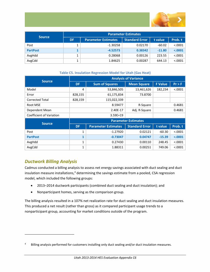
Utah 2013‐2014 HES Evaluation Appendix C6
Source Parameter Estimates
DF Parameter Estimates Standard Error t value Prob. t
Post 1 ‐1.30258 0.02170 ‐60.02 <.0001
PartPost 1 ‐4.52573 0.38342 ‐11.80 <.0001
AvgHdd 1 0.28068 0.00126 223.55 <.0001
AvgCdd 1 1.84625 0.00287 644.13 <.0001
Table C5. Insulation Regression Model for Utah (Gas Heat)
Source Analysis of Variance
DF Sum of Squares Mean Square F Value Pr > F
Model 4 53,846,505 13,461,626 182,234 <.0001
Error 828,155 61,175,834 73.8700
Corrected Total 828,159 115,022,339
Root MSE 8.59477 R‐Square 0.4681
Dependent Mean 2.40E‐17 Adj. R‐Square 0.4681
Coefficient of Variation 3.59E+19
Source Parameter Estimates
DF Parameter Estimates Standard Error t value Prob. t
Post 1 ‐1.27920 0.02121 ‐60.30 <.0001
PartPost 1 ‐0.73047 0.04747 ‐15.39 <.0001
AvgHdd 1 0.27430 0.00110 248.45 <.0001
AvgCdd 1 1.88311 0.00251 749.06 <.0001
Ductwork Billing Analysis Cadmus conducted a billing analysis to assess net energy savings associated with duct sealing and duct
insulation measure installations,4 determining the savings estimate from a pooled, CSA regression
model, which included the following groups:
2013–2014 ductwork participants (combined duct sealing and duct insulation); and
Nonparticipant homes, serving as the comparison group.
The billing analysis resulted in a 107% net realization rate for duct sealing and duct insulation measures.
This produced a net result (rather than gross) as it compared participant usage trends to a
nonparticipant group, accounting for market conditions outside of the program.
4 Billing analysis performed for customers installing only duct sealing and/or duct insulation measures.
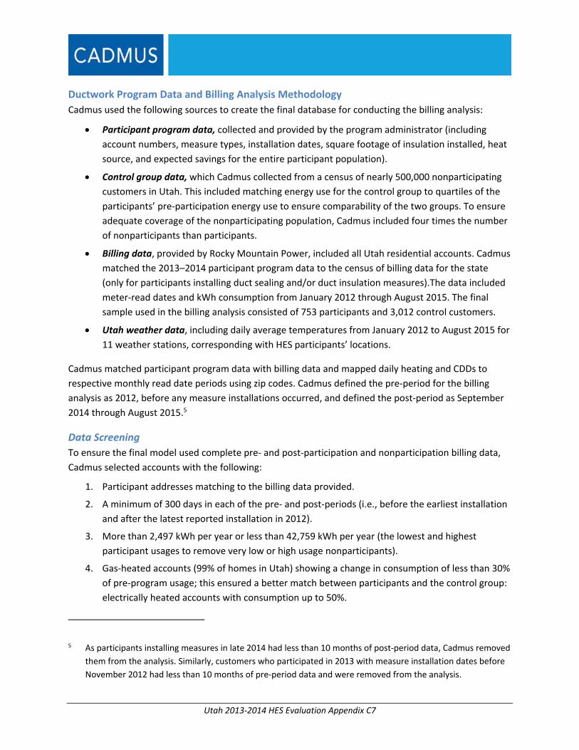
Utah 2013‐2014 HES Evaluation Appendix C7
Ductwork Program Data and Billing Analysis Methodology
Cadmus used the following sources to create the final database for conducting the billing analysis:
Participant program data, collected and provided by the program administrator (including
account numbers, measure types, installation dates, square footage of insulation installed, heat
source, and expected savings for the entire participant population).
Control group data, which Cadmus collected from a census of nearly 500,000 nonparticipating
customers in Utah. This included matching energy use for the control group to quartiles of the
participants’ pre‐participation energy use to ensure comparability of the two groups. To ensure
adequate coverage of the nonparticipating population, Cadmus included four times the number
of nonparticipants than participants.
Billing data, provided by Rocky Mountain Power, included all Utah residential accounts. Cadmus
matched the 2013–2014 participant program data to the census of billing data for the state
(only for participants installing duct sealing and/or duct insulation measures).The data included
meter‐read dates and kWh consumption from January 2012 through August 2015. The final
sample used in the billing analysis consisted of 753 participants and 3,012 control customers.
Utah weather data, including daily average temperatures from January 2012 to August 2015 for
11 weather stations, corresponding with HES participants’ locations.
Cadmus matched participant program data with billing data and mapped daily heating and CDDs to
respective monthly read date periods using zip codes. Cadmus defined the pre‐period for the billing
analysis as 2012, before any measure installations occurred, and defined the post‐period as September
2014 through August 2015.5
Data Screening
To ensure the final model used complete pre‐ and post‐participation and nonparticipation billing data,
Cadmus selected accounts with the following:
1. Participant addresses matching to the billing data provided.
2. A minimum of 300 days in each of the pre‐ and post‐periods (i.e., before the earliest installation
and after the latest reported installation in 2012).
3. More than 2,497 kWh per year or less than 42,759 kWh per year (the lowest and highest
participant usages to remove very low or high usage nonparticipants).
4. Gas‐heated accounts (99% of homes in Utah) showing a change in consumption of less than 30%
of pre‐program usage; this ensured a better match between participants and the control group:
electrically heated accounts with consumption up to 50%.
5 As participants installing measures in late 2014 had less than 10 months of post‐period data, Cadmus removed
them from the analysis. Similarly, customers who participated in 2013 with measure installation dates before
November 2012 had less than 10 months of pre‐period data and were removed from the analysis.
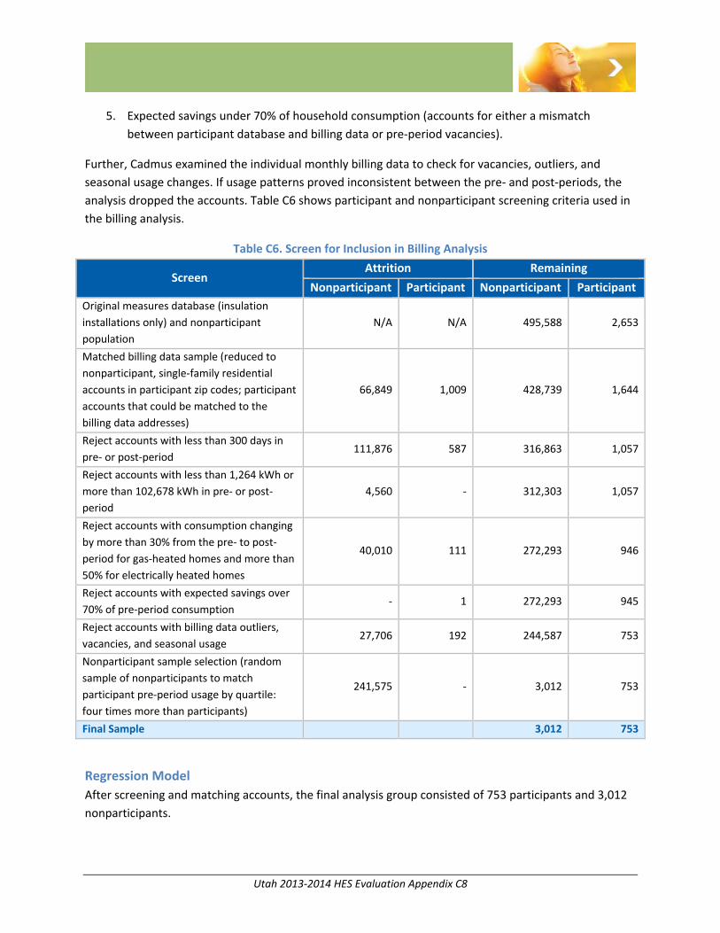
Utah 2013‐2014 HES Evaluation Appendix C8
5. Expected savings under 70% of household consumption (accounts for either a mismatch
between participant database and billing data or pre‐period vacancies).
Further, Cadmus examined the individual monthly billing data to check for vacancies, outliers, and
seasonal usage changes. If usage patterns proved inconsistent between the pre‐ and post‐periods, the
analysis dropped the accounts. Table C6 shows participant and nonparticipant screening criteria used in
the billing analysis.
Table C6. Screen for Inclusion in Billing Analysis
Screen Attrition Remaining
Nonparticipant Participant Nonparticipant Participant
Original measures database (insulation
installations only) and nonparticipant
population
N/A N/A 495,588 2,653
Matched billing data sample (reduced to
nonparticipant, single‐family residential
accounts in participant zip codes; participant
accounts that could be matched to the
billing data addresses)
66,849 1,009 428,739 1,644
Reject accounts with less than 300 days in
pre‐ or post‐period 111,876 587 316,863 1,057
Reject accounts with less than 1,264 kWh or
more than 102,678 kWh in pre‐ or post‐
period
4,560 ‐ 312,303 1,057
Reject accounts with consumption changing
by more than 30% from the pre‐ to post‐
period for gas‐heated homes and more than
50% for electrically heated homes
40,010 111 272,293 946
Reject accounts with expected savings over
70% of pre‐period consumption ‐ 1 272,293 945
Reject accounts with billing data outliers,
vacancies, and seasonal usage 27,706 192 244,587 753
Nonparticipant sample selection (random
sample of nonparticipants to match
participant pre‐period usage by quartile:
four times more than participants)
241,575 ‐ 3,012 753
Final Sample 3,012 753
Regression Model
After screening and matching accounts, the final analysis group consisted of 753 participants and 3,012
nonparticipants.
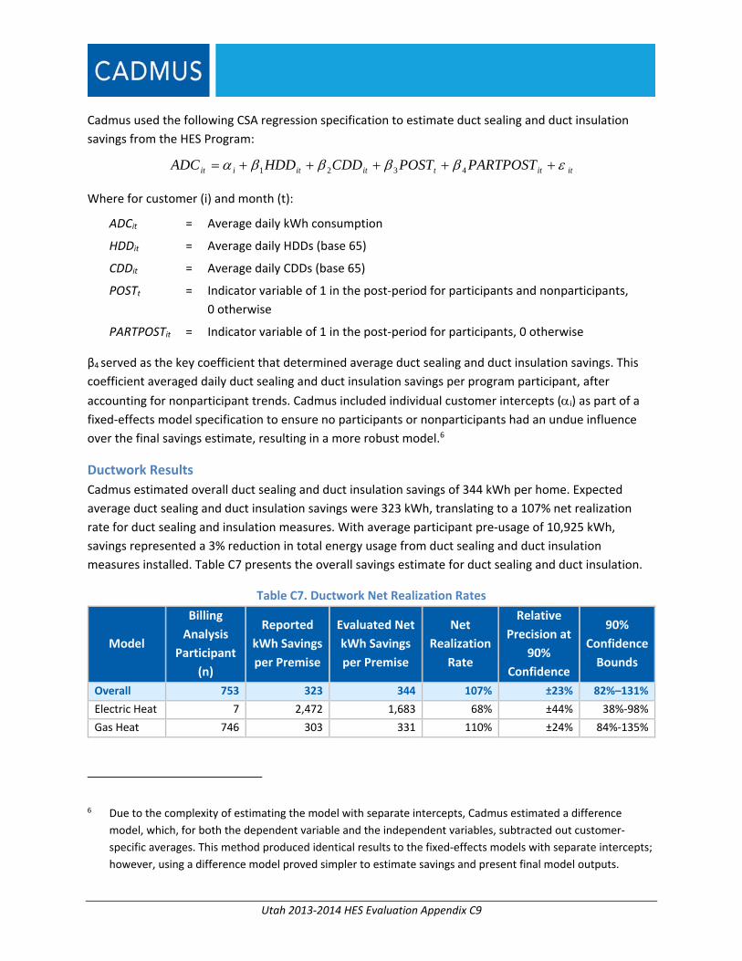
Utah 2013‐2014 HES Evaluation Appendix C9
Cadmus used the following CSA regression specification to estimate duct sealing and duct insulation
savings from the HES Program:
itittititiit PARTPOSTPOSTCDDHDDADC 4321
Where for customer (i) and month (t):
ADCit = Average daily kWh consumption
HDDit = Average daily HDDs (base 65)
CDDit = Average daily CDDs (base 65)
POSTt = Indicator variable of 1 in the post‐period for participants and nonparticipants,
0 otherwise
PARTPOSTit = Indicator variable of 1 in the post‐period for participants, 0 otherwise
β4 served as the key coefficient that determined average duct sealing and duct insulation savings. This
coefficient averaged daily duct sealing and duct insulation savings per program participant, after
accounting for nonparticipant trends. Cadmus included individual customer intercepts (i) as part of a
fixed‐effects model specification to ensure no participants or nonparticipants had an undue influence
over the final savings estimate, resulting in a more robust model.6
Ductwork Results
Cadmus estimated overall duct sealing and duct insulation savings of 344 kWh per home. Expected
average duct sealing and duct insulation savings were 323 kWh, translating to a 107% net realization
rate for duct sealing and insulation measures. With average participant pre‐usage of 10,925 kWh,
savings represented a 3% reduction in total energy usage from duct sealing and duct insulation
measures installed. Table C7 presents the overall savings estimate for duct sealing and duct insulation.
Table C7. Ductwork Net Realization Rates
Model
Billing
Analysis
Participant
(n)
Reported
kWh Savings
per Premise
Evaluated Net
kWh Savings
per Premise
Net
Realization
Rate
Relative
Precision at
90%
Confidence
90%
Confidence
Bounds
Overall 753 323 344 107% ±23% 82%–131%
Electric Heat 7 2,472 1,683 68% ±44% 38%‐98%
Gas Heat 746 303 331 110% ±24% 84%‐135%
6 Due to the complexity of estimating the model with separate intercepts, Cadmus estimated a difference
model, which, for both the dependent variable and the independent variables, subtracted out customer‐
specific averages. This method produced identical results to the fixed‐effects models with separate intercepts;
however, using a difference model proved simpler to estimate savings and present final model outputs.
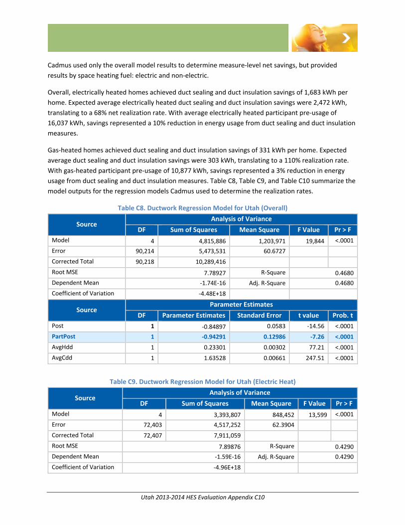
Utah 2013‐2014 HES Evaluation Appendix C10
Cadmus used only the overall model results to determine measure‐level net savings, but provided
results by space heating fuel: electric and non‐electric.
Overall, electrically heated homes achieved duct sealing and duct insulation savings of 1,683 kWh per
home. Expected average electrically heated duct sealing and duct insulation savings were 2,472 kWh,
translating to a 68% net realization rate. With average electrically heated participant pre‐usage of
16,037 kWh, savings represented a 10% reduction in energy usage from duct sealing and duct insulation
measures.
Gas‐heated homes achieved duct sealing and duct insulation savings of 331 kWh per home. Expected
average duct sealing and duct insulation savings were 303 kWh, translating to a 110% realization rate.
With gas‐heated participant pre‐usage of 10,877 kWh, savings represented a 3% reduction in energy
usage from duct sealing and duct insulation measures. Table C8, Table C9, and Table C10 summarize the
model outputs for the regression models Cadmus used to determine the realization rates.
Table C8. Ductwork Regression Model for Utah (Overall)
Source Analysis of Variance
DF Sum of Squares Mean Square F Value Pr > F
Model 4 4,815,886 1,203,971 19,844 <.0001
Error 90,214 5,473,531 60.6727
Corrected Total 90,218 10,289,416
Root MSE 7.78927 R‐Square 0.4680
Dependent Mean ‐1.74E‐16 Adj. R‐Square 0.4680
Coefficient of Variation ‐4.48E+18
Source Parameter Estimates
DF Parameter Estimates Standard Error t value Prob. t
Post 1 ‐0.84897 0.0583 ‐14.56 <.0001
PartPost 1 ‐0.94291 0.12986 ‐7.26 <.0001
AvgHdd 1 0.23301 0.00302 77.21 <.0001
AvgCdd 1 1.63528 0.00661 247.51 <.0001
Table C9. Ductwork Regression Model for Utah (Electric Heat)
Source Analysis of Variance
DF Sum of Squares Mean Square F Value Pr > F
Model 4 3,393,807 848,452 13,599 <.0001
Error 72,403 4,517,252 62.3904
Corrected Total 72,407 7,911,059
Root MSE 7.89876 R‐Square 0.4290
Dependent Mean ‐1.59E‐16 Adj. R‐Square 0.4290
Coefficient of Variation ‐4.96E+18
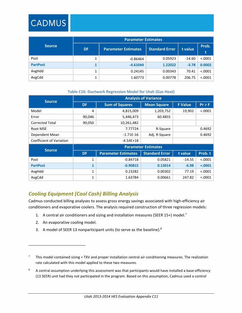
Utah 2013‐2014 HES Evaluation Appendix C11
Source
Parameter Estimates
DF Parameter Estimates Standard Error t value Prob.
t
Post 1 ‐0.86464 0.05923 ‐14.60 <.0001
PartPost 1 ‐4.61044 1.22022 ‐3.78 0.0002
AvgHdd 1 0.24145 0.00343 70.41 <.0001
AvgCdd 1 1.60773 0.00778 206.75 <.0001
Table C10. Ductwork Regression Model for Utah (Gas Heat)
Source Analysis of Variance
DF Sum of Squares Mean Square F Value Pr > F
Model 4 4,815,009 1,203,752 19,902 <.0001
Error 90,046 5,446,473 60.4855
Corrected Total 90,050 10,261,482
Root MSE 7.77724 R‐Square 0.4692
Dependent Mean ‐1.71E‐16 Adj. R‐Square 0.4692
Coefficient of Variation ‐4.54E+18
Source Parameter Estimates
DF Parameter Estimates Standard Error t value Prob. t
Post 1 ‐0.84718 0.05821 ‐14.55 <.0001
PartPost 1 ‐0.90815 0.13014 ‐6.98 <.0001
AvgHdd 1 0.23282 0.00302 77.19 <.0001
AvgCdd 1 1.63784 0.00661 247.82 <.0001
Cooling Equipment (Cool Cash) Billing Analysis Cadmus conducted billing analyses to assess gross energy savings associated with high‐efficiency air
conditioners and evaporative coolers. The analysis required construction of three regression models:
1. A central air conditioners and sizing and installation measures (SEER 15+) model.7
2. An evaporative cooling model.
3. A model of SEER 13 nonparticipant units (to serve as the baseline).8
7 This model contained sizing + TXV and proper installation central air‐conditioning measures. The realization
rate calculated with this model applied to these two measures.
8 A central assumption underlying this assessment was that participants would have installed a base‐efficiency
(13 SEER) unit had they not participated in the program. Based on this assumption, Cadmus used a control
Utah 2013‐2014 HES Evaluation Appendix C12
Cooling Equipment Program Data Billing Analysis Methodology
Cadmus used following regression model to estimate consumption for all three groups:
ADC = + 1 CDD + 2 SQFT +
Where:
ADC = Average daily kWh consumption
CDD = Average daily CDDs
SQFT = Home square feet
The equation determined energy consumption, defined as average daily kWh consumption, by average
daily CDD and home size.
Some estimation error () exists in the regression relationship after accounting for weather and home
size. The 1 coefficient measures energy consumption per CDD. Cadmus estimated average savings for
each of the participating groups (15+ SEER and evaporative cooling models) as the difference between
their respective model coefficient of CDD and the estimated model coefficient of CDD for the 13 SEER
group, multiplied by the average 10‐year CDD for Utah.
The models estimated savings by isolating weather impacts from other factors contributing to energy
consumption. The savings were determined using only 2015 billing data in the cooling season (where
CDD were greater than 0) following their installation of the high‐efficiency unit.9
Cadmus used the following sources to create the final database for conducting the billing analysis:
Participant program data, collected and provided by the program implementer. These data
included account numbers, site addresses, unit types, and installation dates for the entire
participant population.
Billing data, including meter‐read dates, days in billing cycle, and kWh consumption from
January 2012 through August 2015 for all 2013–2014 participants receiving cooling equipment
and control group participants. Rocky Mountain Power only provided billing data for active
residential customer accounts.
group composed of 2005 Cool Cash Program participants known to have received a 13 SEER air‐conditioning
unit—without sizing + TXV or proper installation incentives—as their primary cooling system. SEER 13 air‐
conditioning equipment represented the federal minimum efficiency level for residential central air
conditioners manufactured after January 2006.
9 Cadmus used the entire 2015 cooling season for the program nonparticipant control group.
Utah 2013‐2014 HES Evaluation Appendix C13
Utah weather data, including daily minimum and maximum temperatures and CDDs from
January 2002 to August 2015.
Square footage data, collected by Cadmus through a real estate listing service.10
The billing analysis results provided gross realization rates for central air conditioners and evaporative
cooler equipment types across both years. Cadmus then applied the appropriate equipment‐specific
realization rate to reported savings to determine evaluated gross measure savings estimates.
Cooling Equipment Results
Cadmus used three regression models to estimate program energy savings: SEER 13 (baseline), central
air conditioners and sizing and installation measures (SEER 15+), and evaporative coolers. Cadmus used
billing data from January 2015 through August 2015 to ensure availability of adequate data for
participants receiving an incentive in the early months of 2013 or in the later months of 2014. Prior to
model specification, Cadmus conducted a detailed quality‐assurance review of all available data to
identify missing values or data quality issues; the review found that few data points missing. Following
standard analytical practice, Cadmus screened data for extreme kWh values and eliminated outliers
from the analysis.
The models revealed that several variables could be excluded, primarily those for groups with similar
characteristics. For example, the evaporative coolers model did not incorporate home types and
numbers of stories as these variables highly correlated with square footage, which the model already
included. Further, to increase the number of customers considered for analysis, Cadmus did not include
variables such as whether the occupant completed a recent renovation or added, changed out, or
removed electric appliances in the home.
Table C11 shows the regression model results.11 SEER 13 units’ average consumption per CDD, estimated
at 1.42 kWh, represented the baseline or consumption level occurring in the program’s absence.12
Cadmus used this baseline to estimate savings from each participating central air conditioner and
evaporative cooler unit.
10 http://www.zillow.com/
11 For all three models, the F‐test proved statistically significant. In most instances, parameters for other
independent variables proved significant and had the correct signs. The F‐test determined whether two
population variances were equal by comparing the ratio of their variances. If the variances were equal, the
variances’ ratio would be 1. Typically, this test is used to compare the validity of models.
12 Cadmus considered SEER 13 as the baseline, given that it served as the federal minimum efficiency level for
residential, central air conditioners manufactured after January 2006; thus, it could be assumed to represent
the efficiency of cooling equipment that would have been purchased in the program’s absence.
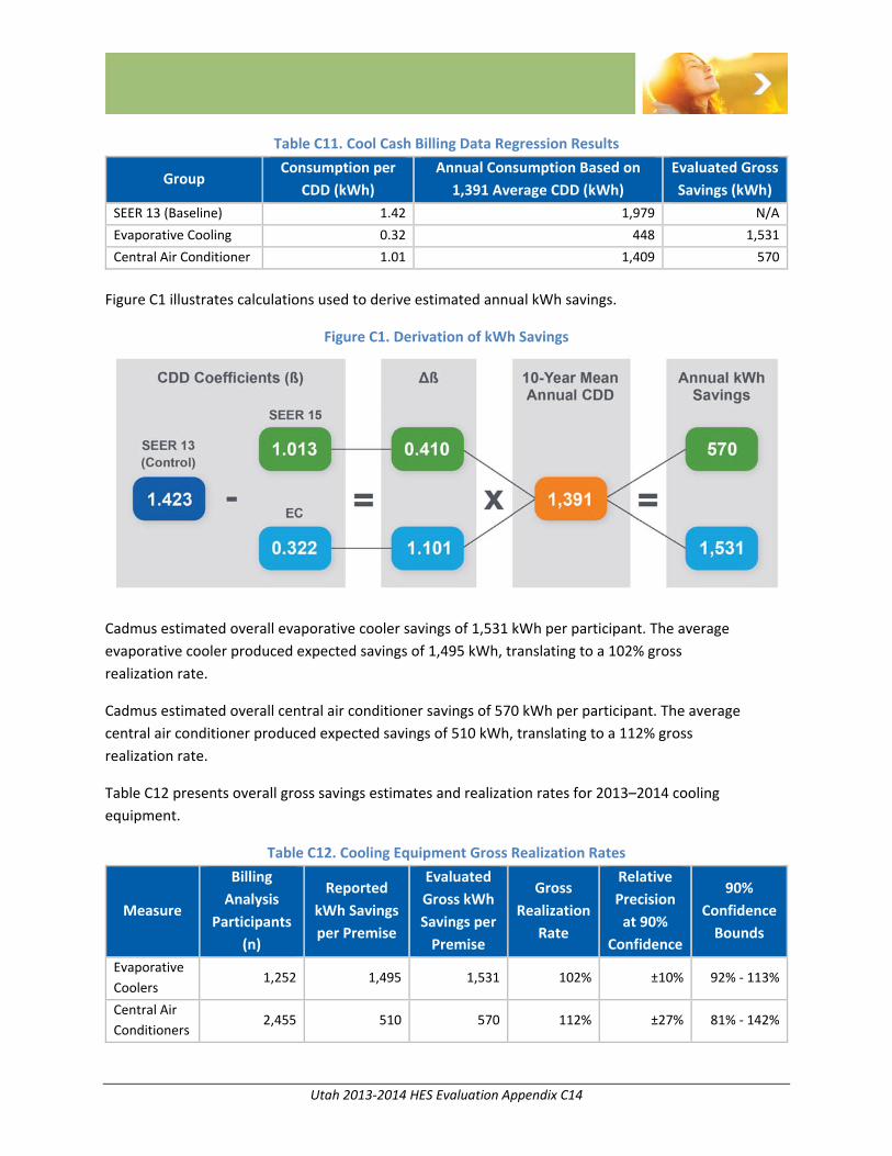
Utah 2013‐2014 HES Evaluation Appendix C14
Table C11. Cool Cash Billing Data Regression Results
Group Consumption per
CDD (kWh)
Annual Consumption Based on
1,391 Average CDD (kWh)
Evaluated Gross
Savings (kWh)
SEER 13 (Baseline) 1.42 1,979 N/A
Evaporative Cooling 0.32 448 1,531
Central Air Conditioner 1.01 1,409 570
Figure C1 illustrates calculations used to derive estimated annual kWh savings.
Figure C1. Derivation of kWh Savings
Cadmus estimated overall evaporative cooler savings of 1,531 kWh per participant. The average
evaporative cooler produced expected savings of 1,495 kWh, translating to a 102% gross
realization rate.
Cadmus estimated overall central air conditioner savings of 570 kWh per participant. The average
central air conditioner produced expected savings of 510 kWh, translating to a 112% gross
realization rate.
Table C12 presents overall gross savings estimates and realization rates for 2013–2014 cooling
equipment.
Table C12. Cooling Equipment Gross Realization Rates
Measure
Billing
Analysis
Participants
(n)
Reported
kWh Savings
per Premise
Evaluated
Gross kWh
Savings per
Premise
Gross
Realization
Rate
Relative
Precision
at 90%
Confidence
90%
Confidence
Bounds
Evaporative
Coolers 1,252 1,495 1,531 102% ±10% 92% ‐ 113%
Central Air
Conditioners 2,455 510 570 112% ±27% 81% ‐ 142%
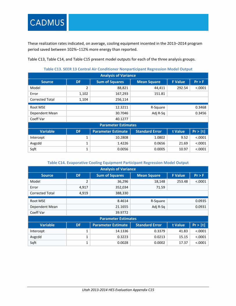
Utah 2013‐2014 HES Evaluation Appendix C15
These realization rates indicated, on average, cooling equipment incented in the 2013–2014 program
period saved between 102%–112% more energy than reported.
Table C13, Table C14, and Table C15 present model outputs for each of the three analysis groups.
Table C13. SEER 13 Central Air Conditioner Nonparticipant Regression Model Output
Analysis of Variance
Source DF Sum of Squares Mean Square F Value Pr > F
Model 2 88,821 44,411 292.54 <.0001
Error 1,102 167,293 151.81
Corrected Total 1,104 256,114
Root MSE 12.3211 R‐Square 0.3468
Dependent Mean 30.7046 Adj R‐Sq 0.3456
Coeff Var 40.1277
Parameter Estimates
Variable DF Parameter Estimate Standard Error t Value Pr > |t|
Intercept 1 10.2808 1.0802 9.52 <.0001
Avgcdd 1 1.4226 0.0656 21.69 <.0001
Sqft 1 0.0056 0.0005 10.97 <.0001
Table C14. Evaporative Cooling Equipment Participant Regression Model Output
Analysis of Variance
Source DF Sum of Squares Mean Square F Value Pr > F
Model 2 36,296 18,148 253.48 <.0001
Error 4,917 352,034 71.59
Corrected Total 4,919 388,330
Root MSE 8.4614 R‐Square 0.0935
Dependent Mean 21.1655 Adj R‐Sq 0.0931
Coeff Var 39.9772
Parameter Estimates
Variable DF Parameter Estimate Standard Error t Value Pr > |t|
Intercept 1 14.1336 0.3379 41.83 <.0001
Avgcdd 1 0.3223 0.0213 15.15 <.0001
Sqft 1 0.0028 0.0002 17.37 <.0001
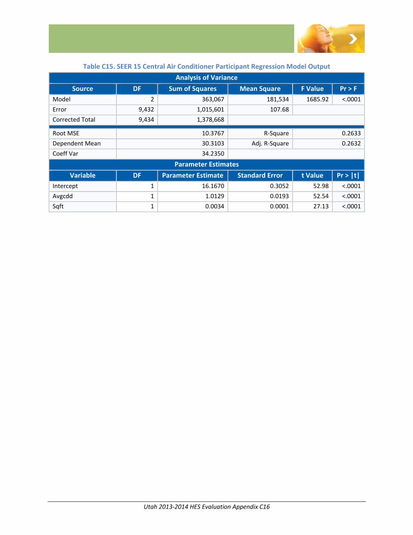
Utah 2013‐2014 HES Evaluation Appendix C16
Table C15. SEER 15 Central Air Conditioner Participant Regression Model Output
Analysis of Variance
Source DF Sum of Squares Mean Square F Value Pr > F
Model 2 363,067 181,534 1685.92 <.0001
Error 9,432 1,015,601 107.68
Corrected Total 9,434 1,378,668
Root MSE 10.3767 R‐Square 0.2633
Dependent Mean 30.3103 Adj. R‐Square 0.2632
Coeff Var 34.2350
Parameter Estimates
Variable DF Parameter Estimate Standard Error t Value Pr > |t|
Intercept 1 16.1670 0.3052 52.98 <.0001
Avgcdd 1 1.0129 0.0193 52.54 <.0001
Sqft 1 0.0034 0.0001 27.13 <.0001

Utah 2013‐2014 HES Evaluation Appendix D1
Appendix D. Self‐Reported Net‐to‐Gross Methodology
Net‐to‐gross (NTG) estimates are a critical part of demand‐side management program impact
evaluations, because they allow utilities to determine portions of gross energy savings that were
influenced by and are attributable to their DSM programs. Freeridership and participant spillover are the
two NTG components calculated in this evaluation. True freeriders are customers who would have
purchased an incented appliance or equipment without any support from the program (e.g. taking the
incentive). Participant spillover is the amount of additional savings obtained by customers investing in
additional energy‐efficient measures or activities due to their program participation. Various methods
can be used to estimate program freeridership and spillover; for this evaluation, Cadmus used self‐
reports from survey participants to estimate NTG for appliances, HVAC and weatherization measure
categories, as this method can gauge net effects for many measures at once and enables Cadmus to
monitor freeridership and spillover over several evaluation efforts.
Survey Design Direct questions (such as: “Would you have installed measure X without the program incentive?”) tend
to result in exaggerated “yes” responses. Participants tend to provide answers they believe surveyors
seek; so a question becomes the equivalent of asking: “Would you have done the right thing on your
own?” An effective solution, and an industry standard, for avoiding such bias involve asking a question in
several different ways, then checking for consistent responses.
Cadmus used industry tested survey questions to determine why customers installed a given measure,
and what influence the program had on their decisions. We used the survey to establish what decision
makers might have done in the program’s absence, via five core freeridership questions:
1. Would participants have installed measures without the program?
2. Had participants ordered or installed the measures before learning about the program?
3. Would participants have installed the measures at the same efficiency levels without the
program incentive?
4. Would participants have installed the same quantity of measures without the program?
5. In the program’s absence, when would respondents have installed the measures?
Cadmus sought to answer three primary questions with our participant spillover survey design:
1. Since participating in the program evaluated, did participants install additional energy‐efficient
equipment or services incented through a utility program?
2. How influential was the evaluated program on the participants’ decisions to install additional
energy‐efficient equipment in their homes?
3. Did customers receive incentives for additional measures installed?
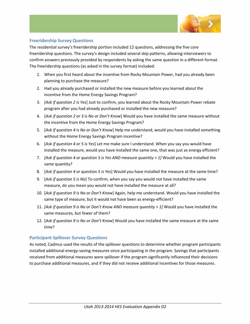
Utah 2013‐2014 HES Evaluation Appendix D2
Freeridership Survey Questions
The residential survey’s freeridership portion included 12 questions, addressing the five core
freeridership questions. The survey’s design included several skip patterns, allowing interviewers to
confirm answers previously provided by respondents by asking the same question in a different format.
The freeridership questions (as asked in the survey format) included:
1. When you first heard about the incentive from Rocky Mountain Power, had you already been
planning to purchase the measure?
2. Had you already purchased or installed the new measure before you learned about the
incentive from the Home Energy Savings Program?
3. [Ask if question 2 is Yes] Just to confirm, you learned about the Rocky Mountain Power rebate
program after you had already purchased or installed the new measure?
4. [Ask if question 2 or 3 is No or Don’t Know] Would you have installed the same measure without
the incentive from the Home Energy Savings Program?
5. [Ask if question 4 is No or Don’t Know] Help me understand, would you have installed something
without the Home Energy Savings Program incentive?
6. [Ask if question 4 or 5 is Yes] Let me make sure I understand. When you say you would have
installed the measure, would you have installed the same one, that was just as energy efficient?
7. [Ask if question 4 or question 5 is Yes AND measure quantity > 1] Would you have installed the
same quantity?
8. [Ask if question 4 or question 5 is Yes] Would you have installed the measure at the same time?
9. [Ask if question 5 is No] To confirm, when you say you would not have installed the same
measure, do you mean you would not have installed the measure at all?
10. [Ask if question 9 is No or Don’t Know] Again, help me understand. Would you have installed the
same type of measure, but it would not have been as energy‐efficient?
11. [Ask if question 9 is No or Don’t Know AND measure quantity > 1] Would you have installed the
same measures, but fewer of them?
12. [Ask if question 9 is No or Don’t Know] Would you have installed the same measure at the same
time?
Participant Spillover Survey Questions
As noted, Cadmus used the results of the spillover questions to determine whether program participants
installed additional energy‐saving measures since participating in the program. Savings that participants
received from additional measures were spillover if the program significantly influenced their decisions
to purchase additional measures, and if they did not receive additional incentives for those measures.

Utah 2013‐2014 HES Evaluation Appendix D3
With the surveys, we specifically asked residential participants whether they installed the following
measures:
Clothes washers
Refrigerators
Dishwashers
Windows
Fixtures
Heat pumps
Ceiling fans
Electric water heaters
CFLs
Insulation
If the participant installed one or more of these measures, we asked additional questions about what
year they purchased the measure, if they received an incentive for the measure, and how influential
(highly influential, somewhat influential, not at all influential) the HES Program was on their purchasing
decisions.
Cadmus combined the freeridership and spillover questions in the same survey, asked over the
telephone with randomly selected program participants. Prior to beginning the survey effort, Cadmus
pre‐tested the survey to ensure that all appropriate prompts and skip patterns were correct. Cadmus
also monitored the survey company’s initial phone calls to verify that:
Survey respondents understood the questions; and
Adjustments were not required.
Freeridership Methodology Cadmus developed a transparent, straightforward matrix for assigning freeridership scores to
participants, based on their responses to targeted survey questions. We assigned a freeridership score
to each question response pattern, and calculated confidence and precision estimates based on the
distribution of these scores (a specific approach cited in the National Action Plan for Energy Efficiency’s
Handbook on DSM Evaluation, 2007 edition, page 5‐1).
Cadmus left the response patterns and scoring weights explicit so that they could be discussed and
changed. We used a rules‐based approach to assign scoring weights to each response from each
freeridership question. This allows for sensitivity analysis to be performed instantaneously and test the
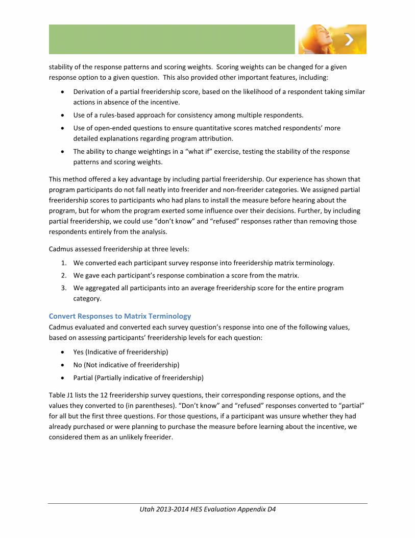
Utah 2013‐2014 HES Evaluation Appendix D4
stability of the response patterns and scoring weights. Scoring weights can be changed for a given
response option to a given question. This also provided other important features, including:
Derivation of a partial freeridership score, based on the likelihood of a respondent taking similar
actions in absence of the incentive.
Use of a rules‐based approach for consistency among multiple respondents.
Use of open‐ended questions to ensure quantitative scores matched respondents’ more
detailed explanations regarding program attribution.
The ability to change weightings in a “what if” exercise, testing the stability of the response
patterns and scoring weights.
This method offered a key advantage by including partial freeridership. Our experience has shown that
program participants do not fall neatly into freerider and non‐freerider categories. We assigned partial
freeridership scores to participants who had plans to install the measure before hearing about the
program, but for whom the program exerted some influence over their decisions. Further, by including
partial freeridership, we could use “don’t know” and “refused” responses rather than removing those
respondents entirely from the analysis.
Cadmus assessed freeridership at three levels:
1. We converted each participant survey response into freeridership matrix terminology.
2. We gave each participant’s response combination a score from the matrix.
3. We aggregated all participants into an average freeridership score for the entire program
category.
Convert Responses to Matrix Terminology
Cadmus evaluated and converted each survey question’s response into one of the following values,
based on assessing participants’ freeridership levels for each question:
Yes (Indicative of freeridership)
No (Not indicative of freeridership)
Partial (Partially indicative of freeridership)
Table J1 lists the 12 freeridership survey questions, their corresponding response options, and the
values they converted to (in parentheses). “Don’t know” and “refused” responses converted to “partial”
for all but the first three questions. For those questions, if a participant was unsure whether they had
already purchased or were planning to purchase the measure before learning about the incentive, we
considered them as an unlikely freerider.
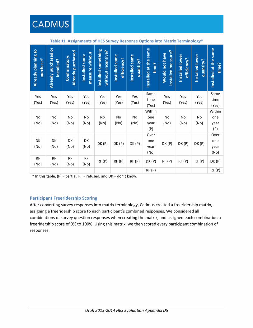
Utah 2013‐2014 HES Evaluation Appendix D5
Table J1. Assignments of HES Survey Response Options into Matrix Terminology*
Alread
y planning to
purchase?
Alread
y purchased or
installed?
Confirm
atory:
Alread
y purchased
Installed sam
e
measure without
Installed something
without incentive?
Installed sam
e
efficiency?
Installed sam
e
quan
tity?
Installed at the sam
e
time?
Would not have
installed m
easure?
Installed lower
efficiency?
Installed lower
quan
tity?
Installed at the sam
e
time?
Yes
(Yes)
Yes
(Yes)
Yes
(Yes)
Yes
(Yes)
Yes
(Yes)
Yes
(Yes)
Yes
(Yes)
Same
time
(Yes)
Yes
(Yes)
Yes
(Yes)
Yes
(Yes)
Same
time
(Yes)
No
(No)
No
(No)
No
(No)
No
(No)
No
(No)
No
(No)
No
(No)
Within
one
year
(P)
No
(No)
No
(No)
No
(No)
Within
one
year
(P)
DK
(No)
DK
(No)
DK
(No)
DK
(No) DK (P) DK (P) DK (P)
Over
one
year
(No)
DK (P) DK (P) DK (P)
Over
one
year
(No)
RF
(No)
RF
(No)
RF
(No)
RF
(No) RF (P) RF (P) RF (P) DK (P) RF (P) RF (P) RF (P) DK (P)
RF (P) RF (P)
* In this table, (P) = partial, RF = refused, and DK = don’t know.
Participant Freeridership Scoring
After converting survey responses into matrix terminology, Cadmus created a freeridership matrix,
assigning a freeridership score to each participant’s combined responses. We considered all
combinations of survey question responses when creating the matrix, and assigned each combination a
freeridership score of 0% to 100%. Using this matrix, we then scored every participant combination of
responses.

Utah 2013‐2014 HES Evaluation Appendix D6
Program Category Freeridership Scoring
After assigning a freeridership score to every survey respondent, Cadmus calculated a savings‐weighted
average freerider score for the program category. We individually weighted each respondent’s freerider
scores by the estimated savings from the equipment they installed, using the following calculation:
∑ ∗ ∑
The Cadmus Freeridership Scoring Model
Cadmus developed an Excel‐based model to use for calculating freeridership, and to improve the
consistency and quality of our results. The model translated raw survey responses into matrix
terminology, and then assigned a matrix score to each participant’s response pattern. Cadmus then
aggregated the program participants into program categories to calculate average freeridership scores.
The model incorporated the following inputs:
Raw survey responses from each participant, along with the program categories for their
incented measures, and their energy savings from those measures, if applicable;
Values converting raw survey responses into matrix terminologies for each program category;
and
Custom freeridership scoring matrices for each unique survey type.
The model displayed each participant’s combination of responses and corresponding freeridership
score, then produced a summary table with the average score and precision estimates for the program
category. The model used the sample size and a two‐tailed test target at the 90% confidence interval to
determine the average score’s precision.
Participant Spillover Methodology For the HES Program, Cadmus measured participant spillover by asking a sample of participants about
their purchases and whether they received an incentive for a particular measure (if they installed
another efficient measure or undertook another energy‐efficiency activity because of their program
participation). We also asked these respondents to rate the HES Program’s (and incentive’s) relative
influence (highly, somewhat, or not at all) on their decisions to pursue additional energy‐efficient
activities.
Participant Spillover Analysis
Cadmus used a top‐down approach to calculate spillover savings. We began our analysis with a subset of
data containing only survey respondents who indicated they installed additional energy‐savings
measures after participating in the HES Program. From this subset, we removed participants who said
the program had little influence on their decisions to purchase additional measures, thus retaining only
participants who rating the program as highly influential. We also removed participants who applied for
an HES incentive for the additional measures they installed.

Utah 2013‐2014 HES Evaluation Appendix D7
For the remaining participants with spillover savings, we estimated the energy savings from additional
measures installed. Cadmus calculated savings values, which we matched to the additional measures
installed by survey participants.
Cadmus calculated the spillover percentage by dividing the sum of additional spillover savings by the
total incentivized gross savings achieved by all respondents in the program category:
% ∑ ∑
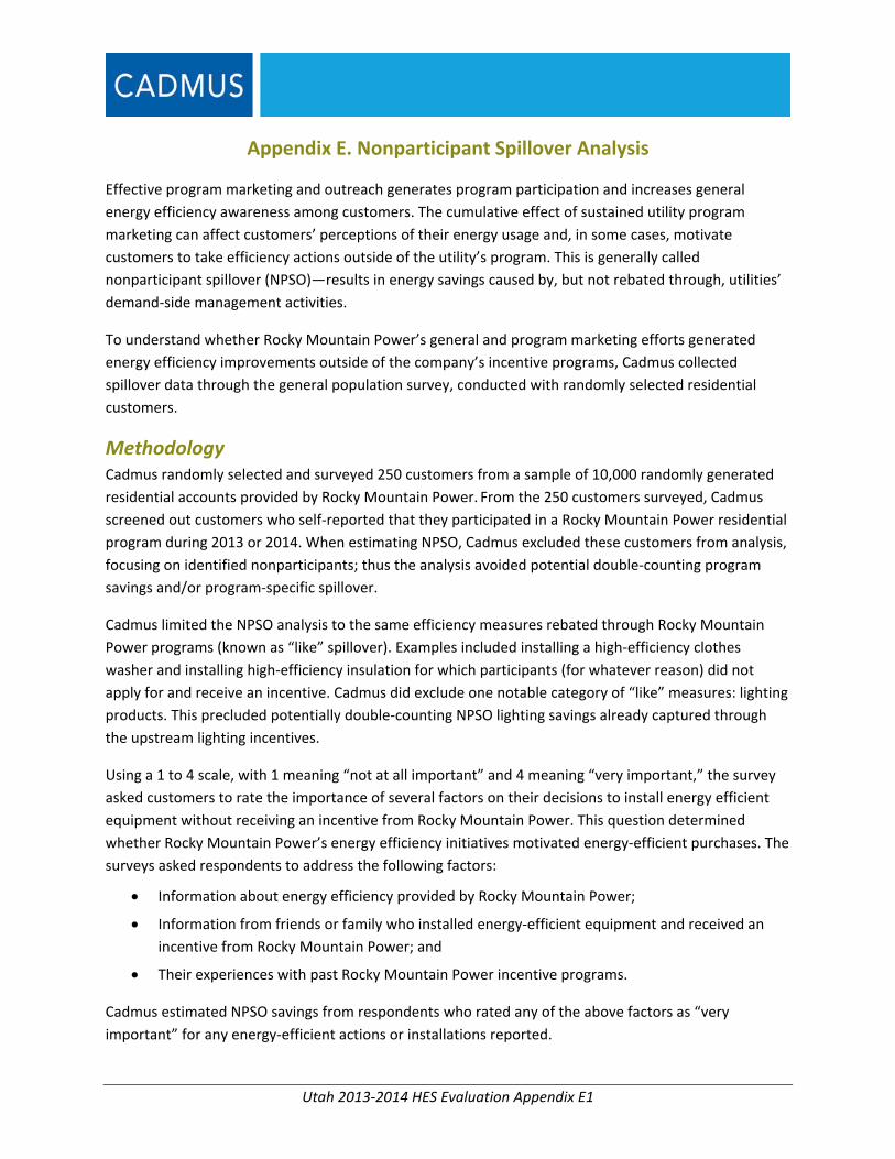
Utah 2013‐2014 HES Evaluation Appendix E1
Appendix E. Nonparticipant Spillover Analysis
Effective program marketing and outreach generates program participation and increases general
energy efficiency awareness among customers. The cumulative effect of sustained utility program
marketing can affect customers’ perceptions of their energy usage and, in some cases, motivate
customers to take efficiency actions outside of the utility’s program. This is generally called
nonparticipant spillover (NPSO)—results in energy savings caused by, but not rebated through, utilities’
demand‐side management activities.
To understand whether Rocky Mountain Power’s general and program marketing efforts generated
energy efficiency improvements outside of the company’s incentive programs, Cadmus collected
spillover data through the general population survey, conducted with randomly selected residential
customers.
Methodology Cadmus randomly selected and surveyed 250 customers from a sample of 10,000 randomly generated
residential accounts provided by Rocky Mountain Power. From the 250 customers surveyed, Cadmus
screened out customers who self‐reported that they participated in a Rocky Mountain Power residential
program during 2013 or 2014. When estimating NPSO, Cadmus excluded these customers from analysis,
focusing on identified nonparticipants; thus the analysis avoided potential double‐counting program
savings and/or program‐specific spillover.
Cadmus limited the NPSO analysis to the same efficiency measures rebated through Rocky Mountain
Power programs (known as “like” spillover). Examples included installing a high‐efficiency clothes
washer and installing high‐efficiency insulation for which participants (for whatever reason) did not
apply for and receive an incentive. Cadmus did exclude one notable category of “like” measures: lighting
products. This precluded potentially double‐counting NPSO lighting savings already captured through
the upstream lighting incentives.
Using a 1 to 4 scale, with 1 meaning “not at all important” and 4 meaning “very important,” the survey
asked customers to rate the importance of several factors on their decisions to install energy efficient
equipment without receiving an incentive from Rocky Mountain Power. This question determined
whether Rocky Mountain Power’s energy efficiency initiatives motivated energy‐efficient purchases. The
surveys asked respondents to address the following factors:
Information about energy efficiency provided by Rocky Mountain Power;
Information from friends or family who installed energy‐efficient equipment and received an
incentive from Rocky Mountain Power; and
Their experiences with past Rocky Mountain Power incentive programs.
Cadmus estimated NPSO savings from respondents who rated any of the above factors as “very
important” for any energy‐efficient actions or installations reported.
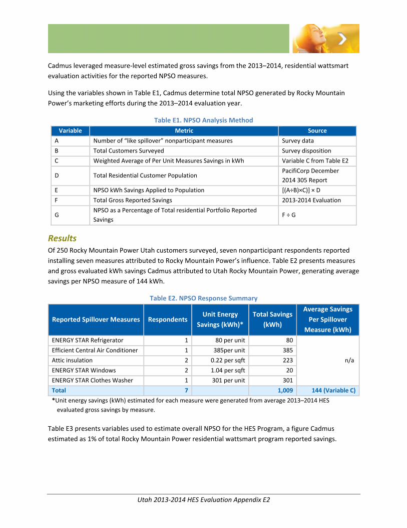
Utah 2013‐2014 HES Evaluation Appendix E2
Cadmus leveraged measure‐level estimated gross savings from the 2013–2014, residential wattsmart
evaluation activities for the reported NPSO measures.
Using the variables shown in Table E1, Cadmus determine total NPSO generated by Rocky Mountain
Power’s marketing efforts during the 2013–2014 evaluation year.
Table E1. NPSO Analysis Method
Variable Metric Source
A Number of “like spillover” nonparticipant measures Survey data
B Total Customers Surveyed Survey disposition
C Weighted Average of Per Unit Measures Savings in kWh Variable C from Table E2
D Total Residential Customer Population PacifiCorp December
2014 305 Report
E NPSO kWh Savings Applied to Population [(A÷B)×C)] × D
F Total Gross Reported Savings 2013‐2014 Evaluation
G NPSO as a Percentage of Total residential Portfolio Reported
Savings F ÷ G
Results Of 250 Rocky Mountain Power Utah customers surveyed, seven nonparticipant respondents reported
installing seven measures attributed to Rocky Mountain Power’s influence. Table E2 presents measures
and gross evaluated kWh savings Cadmus attributed to Utah Rocky Mountain Power, generating average
savings per NPSO measure of 144 kWh.
Table E2. NPSO Response Summary
Reported Spillover Measures Respondents Unit Energy
Savings (kWh)*
Total Savings
(kWh)
Average Savings
Per Spillover
Measure (kWh)
ENERGY STAR Refrigerator 1 80 per unit 80
n/a
Efficient Central Air Conditioner 1 385per unit 385
Attic insulation 2 0.22 per sqft 223
ENERGY STAR Windows 2 1.04 per sqft 20
ENERGY STAR Clothes Washer 1 301 per unit 301
Total 7 1,009 144 (Variable C)
*Unit energy savings (kWh) estimated for each measure were generated from average 2013–2014 HES
evaluated gross savings by measure.
Table E3 presents variables used to estimate overall NPSO for the HES Program, a figure Cadmus
estimated as 1% of total Rocky Mountain Power residential wattsmart program reported savings.
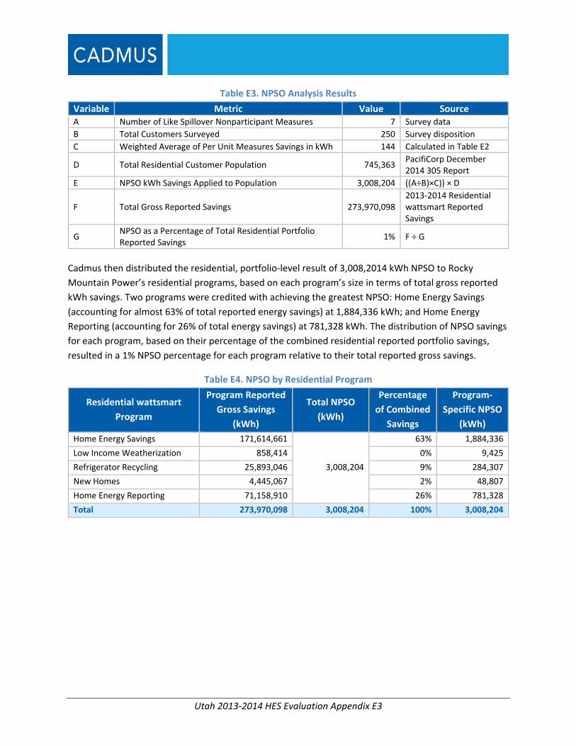
Utah 2013‐2014 HES Evaluation Appendix E3
Table E3. NPSO Analysis Results
Variable Metric Value Source A Number of Like Spillover Nonparticipant Measures 7 Survey data
B Total Customers Surveyed 250 Survey disposition
C Weighted Average of Per Unit Measures Savings in kWh 144 Calculated in Table E2
D Total Residential Customer Population 745,363PacifiCorp December 2014 305 Report
E NPSO kWh Savings Applied to Population 3,008,204 ((A÷B)×C)) × D
F Total Gross Reported Savings 273,970,0982013‐2014 Residentialwattsmart Reported Savings
G NPSO as a Percentage of Total Residential Portfolio Reported Savings
1% F ÷ G
Cadmus then distributed the residential, portfolio‐level result of 3,008,2014 kWh NPSO to Rocky
Mountain Power’s residential programs, based on each program’s size in terms of total gross reported
kWh savings. Two programs were credited with achieving the greatest NPSO: Home Energy Savings
(accounting for almost 63% of total reported energy savings) at 1,884,336 kWh; and Home Energy
Reporting (accounting for 26% of total energy savings) at 781,328 kWh. The distribution of NPSO savings
for each program, based on their percentage of the combined residential reported portfolio savings,
resulted in a 1% NPSO percentage for each program relative to their total reported gross savings.
Table E4. NPSO by Residential Program
Residential wattsmart
Program
Program Reported
Gross Savings
(kWh)
Total NPSO
(kWh)
Percentage
of Combined
Savings
Program‐
Specific NPSO
(kWh)
Home Energy Savings 171,614,661
3,008,204
63% 1,884,336
Low Income Weatherization 858,414 0% 9,425
Refrigerator Recycling 25,893,046 9% 284,307
New Homes 4,445,067 2% 48,807
Home Energy Reporting 71,158,910 26% 781,328
Total 273,970,098 3,008,204 100% 3,008,204
Utah 2013‐2014 HES Evaluation Appendix F1
Appendix F. Lighting Retailer Allocation Review
Rocky Mountain Power subsidizes CFL and LED costs throughout its service territory. As shown in the
leakage study findings (main report), some individuals who are not Rocky Mountain Power customers
benefit from the program. These discounted bulbs “leak” outside of the service territory.
Cadmus met with the program administrator in early October 2015 to review the RSAT and any updates
made since last year’s analysis. Overall, the process of calculating a store’s RSAT score followed the
same process outlined below. Updates included streamlining a number of data processing steps to
reduce the likelihood of human error. In addition, the tool can now handle LED purchases.
The program administrator developed a screening process to minimize the number of leaked bulbs.
Using a proprietary RSAT1 and Buxton Company’s MicroMarketer2 software, the program administrator
only targeted stores where 90% or more of CFL purchases could be attributed to Rocky Mountain Power
customers.
Through a series of meetings, e‐mail exchanges, and software documentation reviews, Cadmus
evaluated the program administrator’s process for reducing CFL and LED leakage. This section outlines
six key aspects of this:
1. Retail customer drive‐time calculation.
2. Retailer locations.
3. Retailer trade areas.
4. Rocky Mountain Power’s service territory.
5. Customer purchasing power.
6. Retail sales allocation.
Retail Customer Drive‐Time Calculation The time a customer willingly takes to drive to purchase efficient lighting from a brick‐and‐motor store
greatly impacts the degree of leakage. Partnering with the Buxton Company, the program administrator
determined three main factors that affected customer drive times: retail class, products sold, and urban
density.
Retail Class
The program administrator/Buxton Company research indicated store types affect customer drive times.
For example, customers commonly drive farther to a Costco than to a local hardware store. The program
1 http://www.peci.org/retail‐sales‐allocation‐tool
2 Buxton specializes in retailer analysis and customer profiling: http://buxtonco.com/
Utah 2013‐2014 HES Evaluation Appendix F2
administrator divided the retailer list into five classes (classes A through F), based on the North
American Industry Classification System (NAICS).3 Table F1 provides examples of NAICS classes.
Table F1. NAICS Classification Examples
NAICS Code NAICS Title
44411 Home Centers
44413 Hardware Stores
443141 Household Appliance Stores
Products Sold
The program administrator categorized products sold by retailers into three classes: White Goods; Over
the Counter (Retrofit); and Over the Counter (Plug and Play).4 CFLs fell within the last of these
categories.
Urban Density
The program administrator assigned stores with an urban or rural designation, based on the Buxton
Urban Density Score (BUDS), which examines population per square foot to account for population
density changes when moving farther from an urban center.
The program administrator modeled the 30 possible drive time factor combinations with over 500,000
survey responses from seven states to establish the amount of time customers drove for a given product
and store type. Figure F1 reflects the drive time results capturing 80% of product sales for a particular
retail class.
3 http://www.census.gov/eos/www/naics/
4 White Goods include clothes washers, refrigerators, and freezers. Characterized as major purchases, customers usually undertake a degree of product research and/or assistance from a store sales person. Over the Counter (Retrofit) includes lighting fixtures (both CFLs and LEDs) and lighting controls. Characterized as midrange cost ($20–$200) products, the category sells as over‐the‐counter home improvement or retrofit products. Over the Counter (Plug and Play) includes bulbs (both CFLs and LEDs) and showerheads. Characterized as low‐cost ($1–$20) products, this category sells through a variety of store types; an average consumer can reasonably install these products without assistance.

Utah 2013‐2014 HES Evaluation Appendix F3
Figure F1. Example of Product Drive‐Time Calculation
Table F2 summarizes the program administrator’s calculated drive times by retail class and
product type.
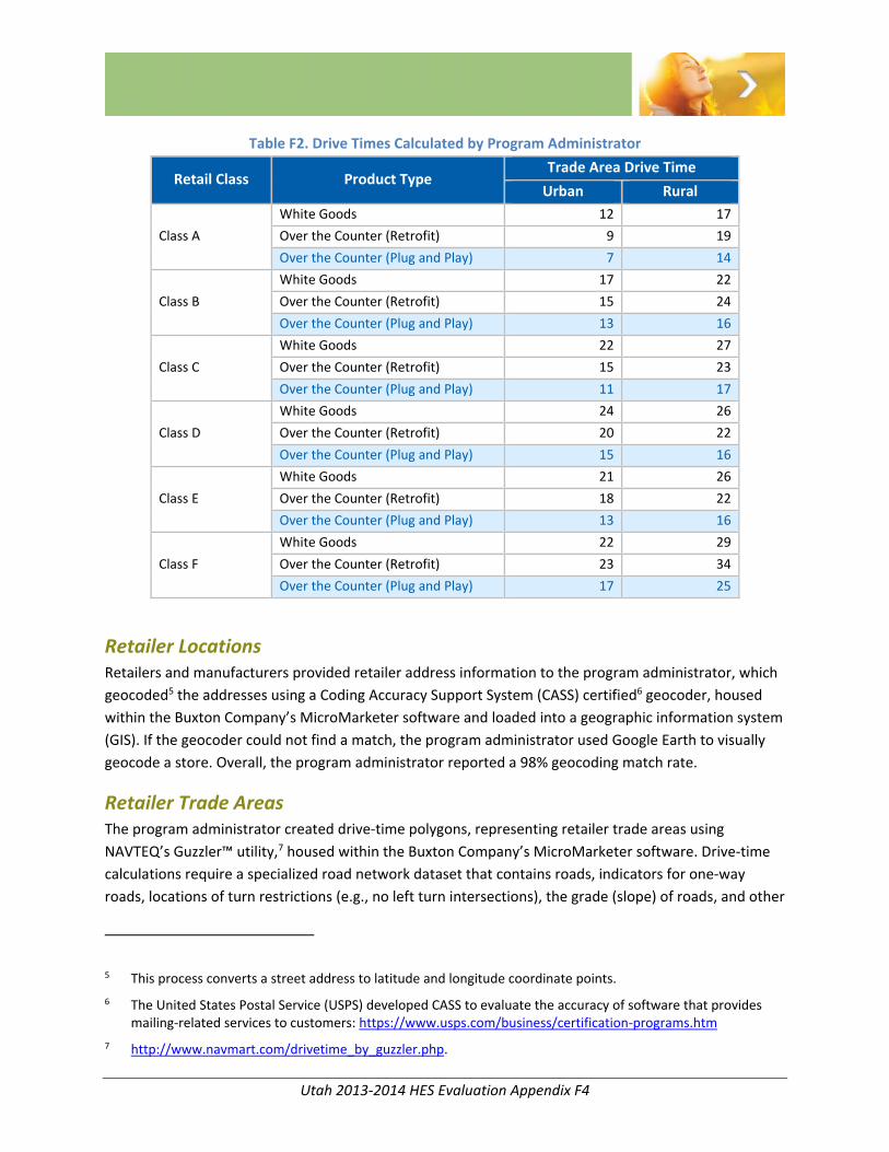
Utah 2013‐2014 HES Evaluation Appendix F4
Table F2. Drive Times Calculated by Program Administrator
Retail Class Product Type Trade Area Drive Time
Urban Rural
Class A
White Goods 12 17
Over the Counter (Retrofit) 9 19
Over the Counter (Plug and Play) 7 14
Class B
White Goods 17 22
Over the Counter (Retrofit) 15 24
Over the Counter (Plug and Play) 13 16
Class C
White Goods 22 27
Over the Counter (Retrofit) 15 23
Over the Counter (Plug and Play) 11 17
Class D
White Goods 24 26
Over the Counter (Retrofit) 20 22
Over the Counter (Plug and Play) 15 16
Class E
White Goods 21 26
Over the Counter (Retrofit) 18 22
Over the Counter (Plug and Play) 13 16
Class F
White Goods 22 29
Over the Counter (Retrofit) 23 34
Over the Counter (Plug and Play) 17 25
Retailer Locations Retailers and manufacturers provided retailer address information to the program administrator, which
geocoded5 the addresses using a Coding Accuracy Support System (CASS) certified6 geocoder, housed
within the Buxton Company’s MicroMarketer software and loaded into a geographic information system
(GIS). If the geocoder could not find a match, the program administrator used Google Earth to visually
geocode a store. Overall, the program administrator reported a 98% geocoding match rate.
Retailer Trade Areas The program administrator created drive‐time polygons, representing retailer trade areas using
NAVTEQ’s Guzzler™ utility,7 housed within the Buxton Company’s MicroMarketer software. Drive‐time
calculations require a specialized road network dataset that contains roads, indicators for one‐way
roads, locations of turn restrictions (e.g., no left turn intersections), the grade (slope) of roads, and other
5 This process converts a street address to latitude and longitude coordinate points.
6 The United States Postal Service (USPS) developed CASS to evaluate the accuracy of software that provides mailing‐related services to customers: https://www.usps.com/business/certification‐programs.htm
7 http://www.navmart.com/drivetime_by_guzzler.php.
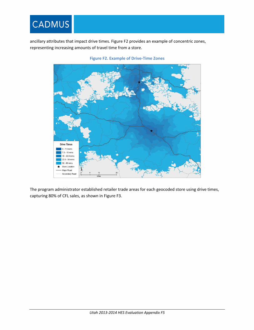
Utah 2013‐2014 HES Evaluation Appendix F5
ancillary attributes that impact drive times. Figure F2 provides an example of concentric zones,
representing increasing amounts of travel time from a store.
Figure F2. Example of Drive‐Time Zones
The program administrator established retailer trade areas for each geocoded store using drive times,
capturing 80% of CFL sales, as shown in Figure F3.
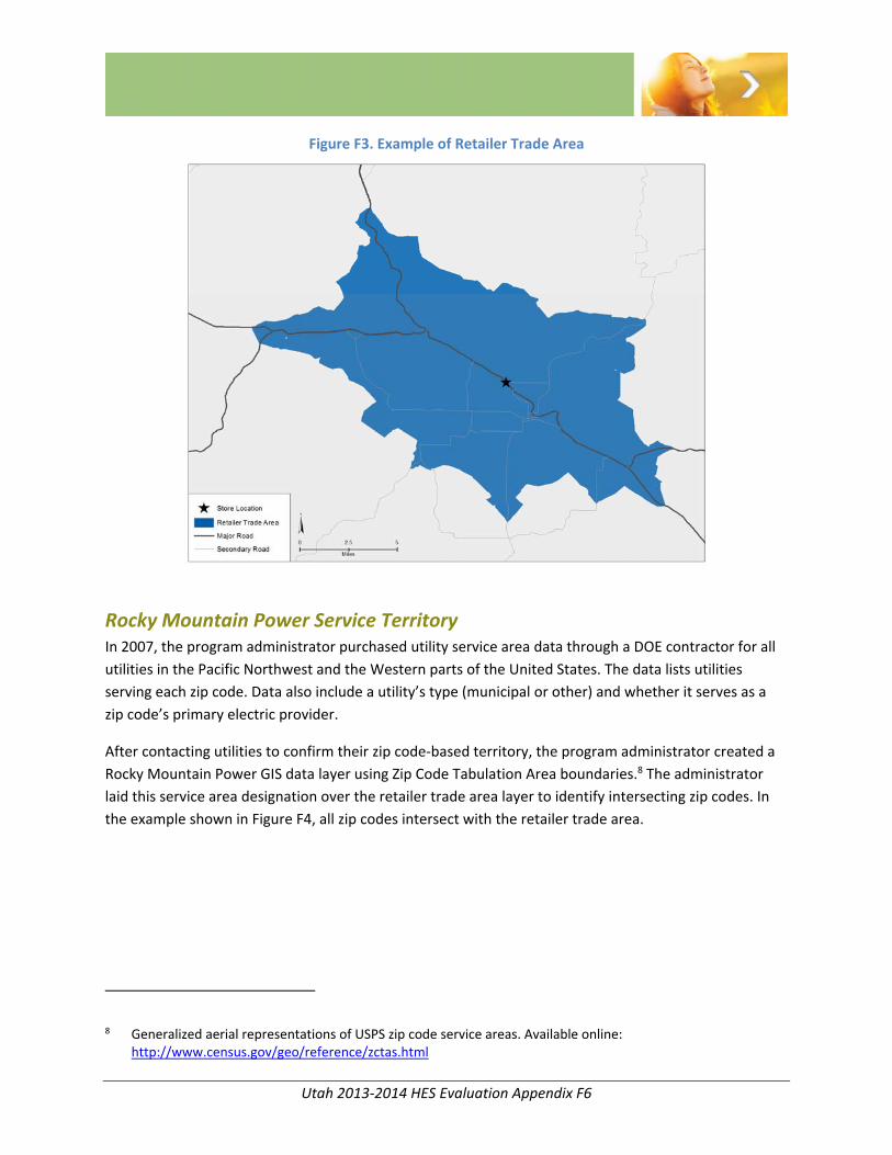
Utah 2013‐2014 HES Evaluation Appendix F6
Figure F3. Example of Retailer Trade Area
Rocky Mountain Power Service Territory In 2007, the program administrator purchased utility service area data through a DOE contractor for all
utilities in the Pacific Northwest and the Western parts of the United States. The data lists utilities
serving each zip code. Data also include a utility’s type (municipal or other) and whether it serves as a
zip code’s primary electric provider.
After contacting utilities to confirm their zip code‐based territory, the program administrator created a
Rocky Mountain Power GIS data layer using Zip Code Tabulation Area boundaries.8 The administrator
laid this service area designation over the retailer trade area layer to identify intersecting zip codes. In
the example shown in Figure F4, all zip codes intersect with the retailer trade area.
8 Generalized aerial representations of USPS zip code service areas. Available online: http://www.census.gov/geo/reference/zctas.html
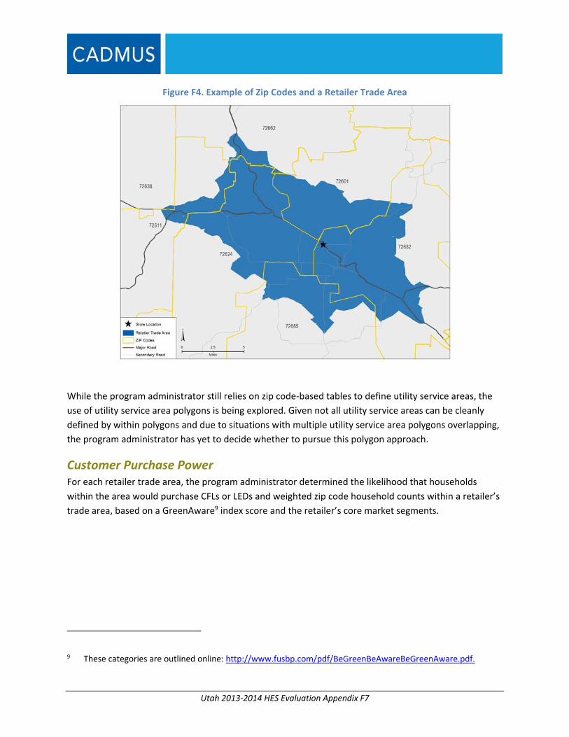
Utah 2013‐2014 HES Evaluation Appendix F7
Figure F4. Example of Zip Codes and a Retailer Trade Area
While the program administrator still relies on zip code‐based tables to define utility service areas, the
use of utility service area polygons is being explored. Given not all utility service areas can be cleanly
defined by within polygons and due to situations with multiple utility service area polygons overlapping,
the program administrator has yet to decide whether to pursue this polygon approach.
Customer Purchase Power For each retailer trade area, the program administrator determined the likelihood that households
within the area would purchase CFLs or LEDs and weighted zip code household counts within a retailer’s
trade area, based on a GreenAware9 index score and the retailer’s core market segments.
9 These categories are outlined online: http://www.fusbp.com/pdf/BeGreenBeAwareBeGreenAware.pdf.
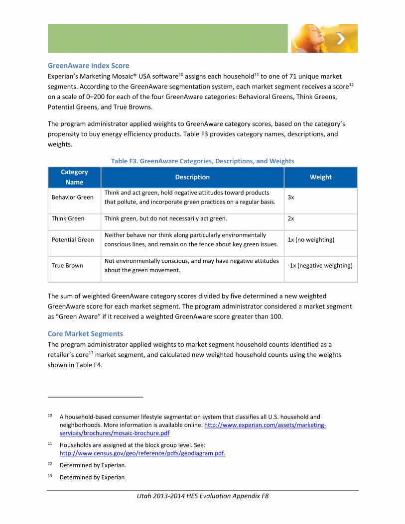
Utah 2013‐2014 HES Evaluation Appendix F8
GreenAware Index Score
Experian’s Marketing Mosaic® USA software10 assigns each household11 to one of 71 unique market
segments. According to the GreenAware segmentation system, each market segment receives a score12
on a scale of 0–200 for each of the four GreenAware categories: Behavioral Greens, Think Greens,
Potential Greens, and True Browns.
The program administrator applied weights to GreenAware category scores, based on the category’s
propensity to buy energy efficiency products. Table F3 provides category names, descriptions, and
weights.
Table F3. GreenAware Categories, Descriptions, and Weights
Category
Name Description Weight
Behavior Green Think and act green, hold negative attitudes toward products
that pollute, and incorporate green practices on a regular basis. 3x
Think Green Think green, but do not necessarily act green. 2x
Potential Green Neither behave nor think along particularly environmentally
conscious lines, and remain on the fence about key green issues. 1x (no weighting)
True Brown Not environmentally conscious, and may have negative attitudes
about the green movement. ‐1x (negative weighting)
The sum of weighted GreenAware category scores divided by five determined a new weighted
GreenAware score for each market segment. The program administrator considered a market segment
as “Green Aware” if it received a weighted GreenAware score greater than 100.
Core Market Segments
The program administrator applied weights to market segment household counts identified as a
retailer’s core13 market segment, and calculated new weighted household counts using the weights
shown in Table F4.
10 A household‐based consumer lifestyle segmentation system that classifies all U.S. household and neighborhoods. More information is available online: http://www.experian.com/assets/marketing‐services/brochures/mosaic‐brochure.pdf
11 Households are assigned at the block group level. See: http://www.census.gov/geo/reference/pdfs/geodiagram.pdf.
12 Determined by Experian.
13 Determined by Experian.
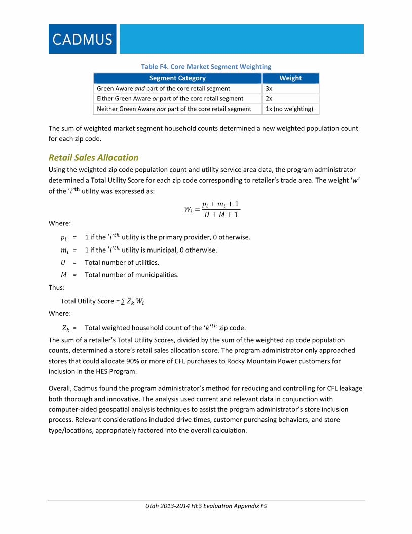
Utah 2013‐2014 HES Evaluation Appendix F9
Table F4. Core Market Segment Weighting
Segment Category Weight
Green Aware and part of the core retail segment 3x
Either Green Aware or part of the core retail segment 2x
Neither Green Aware nor part of the core retail segment 1x (no weighting)
The sum of weighted market segment household counts determined a new weighted population count
for each zip code.
Retail Sales Allocation Using the weighted zip code population count and utility service area data, the program administrator
determined a Total Utility Score for each zip code corresponding to retailer’s trade area. The weight ‘w’
of the ′ ′ utility was expressed as:
11
Where:
= 1 if the ′ ′ utility is the primary provider, 0 otherwise.
= 1 if the ′ ′ utility is municipal, 0 otherwise.
= Total number of utilities.
= Total number of municipalities.
Thus:
Total Utility Score = ∑
Where:
= Total weighted household count of the ‘ ′ zip code.
The sum of a retailer’s Total Utility Scores, divided by the sum of the weighted zip code population
counts, determined a store’s retail sales allocation score. The program administrator only approached
stores that could allocate 90% or more of CFL purchases to Rocky Mountain Power customers for
inclusion in the HES Program.
Overall, Cadmus found the program administrator’s method for reducing and controlling for CFL leakage
both thorough and innovative. The analysis used current and relevant data in conjunction with
computer‐aided geospatial analysis techniques to assist the program administrator’s store inclusion
process. Relevant considerations included drive times, customer purchasing behaviors, and store
type/locations, appropriately factored into the overall calculation.

Utah 2013‐2014 HES Evaluation Appendix G1
Appendix G. Utah Measure Category Cost‐Effectiveness
Completed at the measure category level, cost‐effectiveness was reported for evaluated net savings.
Net results apply the evaluated NTG to evaluated gross savings. Table G1 shows cost‐effectiveness
inputs for net results.
Table G1. Utah Measure Category Cost‐Effectiveness Inputs
Input Description 2013 2014 Total
Average Measure Life*
Appliance 15 15 15
HVAC 18 17 17
Lighting 7 7 7
Weatherization 30 30 30
Evaluated Net Energy Savings (kWh/year)**
Appliance 5,256,138 14,639,289 19,895,427
HVAC 4,567,430 6,569,044 11,136,474
Lighting 46,421,125 26,042,716 72,463,841
Weatherization 4,265,450 3,381,369 7,646,818
Total Utility Cost (including incentives)***
Appliance $3,608,043 $12,410,272 $16,018,314
HVAC $2,938,066 $4,165,710 $7,103,776
Lighting $10,373,380 $6,371,992 $16,745,372
Weatherization $3,872,815 $3,222,701 $7,095,516
Incentives
Appliance $3,091,539 $10,704,362 $13,795,901
HVAC $2,418,606 $3,303,377 $5,721,983
Lighting $7,648,443 $4,462,648 $12,111,091
Weatherization $3,163,188 $2,568,748 $5,731,936
Retail Rate $0.1056 $0.1084 N/A
*Weighted average measure category lives are based on individual measure lifetimes and
weighted by savings and the frequency of installations.
**Evaluated savings reflect impacts at the customer meter.
***Rocky Mountain Power provided program costs and incentives in annual report data,
allocating program costs by weighted savings.

Utah 2013‐2014 HES Evaluation Appendix G2
Appliances Cost‐effectiveness results for net savings are shown in Table G2, Table G3, and Table G4. The appliance
measure category proved cost‐effective from all perspectives except for the RIM (Table G2).
Table G2. Utah Appliance 2013‐2014 Net (2013 IRP East Residential Whole House 35% Medium LF Decrement)
Cost‐Effectiveness Test Levelized
$/kWh Costs Benefits Net Benefits
Benefit/Cost
Ratio
PTRC (TRC + 10% Conservation
Adder) $0.062 $12,471,888 $18,145,911 $5,674,023 1.45
TRC $0.062 $12,471,888 $16,496,719 $4,024,831 1.32
UCT $0.076 $15,224,029 $16,496,719 $1,272,690 1.08
RIM $37,206,262 $16,503,121 ($20,703,142) 0.44
PCT $12,791,261 $39,824,850 $27,033,589 3.11
Lifecycle Revenue Impacts ($/kWh) $0.000064094
Discounted Participant Payback
(years) 1.72
Table G3. Utah Appliance 2013 Net (2013 IRP East Residential Whole House 35% Medium LF Decrement)
Cost‐Effectiveness Test Levelized
$/kWh Costs Benefits
Net
Benefits
Benefit/Cost
Ratio
PTRC (TRC + 10% Conservation
Adder) $0.076 $4,207,735 $4,847,527 $639,792 1.15
TRC $0.076 $4,207,735 $4,406,843 $199,107 1.05
UCT $0.065 $3,608,043 $4,406,843 $798,800 1.22
RIM $9,451,286 $4,406,843 ($5,044,444) 0.47
PCT $4,557,076 $10,305,420 $5,748,344 2.26
Lifecycle Revenue Impacts ($/kWh) $0.000016072
Discounted Participant Payback
(years) 2.23
Table G4. Utah Appliance 2014 Net (2013 IRP East Residential Whole House 35% Medium LF Decrement)
Cost‐Effectiveness Test Levelized
$/kWh Costs Benefits Net Benefits
Benefit/Cost
Ratio
PTRC (TRC + 10% Conservation
Adder) $0.057 $8,832,892 $14,213,579 $5,380,687 1.61
TRC $0.057 $8,832,892 $12,921,901 $4,089,010 1.46
UCT $0.080 $12,415,398 $12,921,901 $506,503 1.04
RIM $29,665,073 $12,928,744 ($16,736,330) 0.44
PCT $8,800,862 $32,000,257 $23,199,396 3.64
Lifecycle Revenue Impacts ($/kWh) $0.000052232
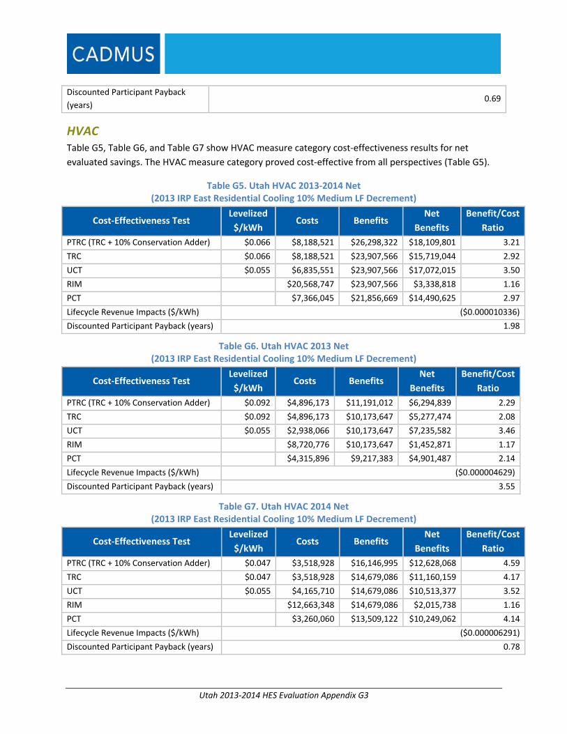
Utah 2013‐2014 HES Evaluation Appendix G3
Discounted Participant Payback
(years) 0.69
HVAC Table G5, Table G6, and Table G7 show HVAC measure category cost‐effectiveness results for net
evaluated savings. The HVAC measure category proved cost‐effective from all perspectives (Table G5).
Table G5. Utah HVAC 2013‐2014 Net (2013 IRP East Residential Cooling 10% Medium LF Decrement)
Cost‐Effectiveness Test Levelized
$/kWh Costs Benefits
Net
Benefits
Benefit/Cost
Ratio
PTRC (TRC + 10% Conservation Adder) $0.066 $8,188,521 $26,298,322 $18,109,801 3.21
TRC $0.066 $8,188,521 $23,907,566 $15,719,044 2.92
UCT $0.055 $6,835,551 $23,907,566 $17,072,015 3.50
RIM $20,568,747 $23,907,566 $3,338,818 1.16
PCT $7,366,045 $21,856,669 $14,490,625 2.97
Lifecycle Revenue Impacts ($/kWh) ($0.000010336)
Discounted Participant Payback (years) 1.98
Table G6. Utah HVAC 2013 Net (2013 IRP East Residential Cooling 10% Medium LF Decrement)
Cost‐Effectiveness Test Levelized
$/kWh Costs Benefits
Net
Benefits
Benefit/Cost
Ratio
PTRC (TRC + 10% Conservation Adder) $0.092 $4,896,173 $11,191,012 $6,294,839 2.29
TRC $0.092 $4,896,173 $10,173,647 $5,277,474 2.08
UCT $0.055 $2,938,066 $10,173,647 $7,235,582 3.46
RIM $8,720,776 $10,173,647 $1,452,871 1.17
PCT $4,315,896 $9,217,383 $4,901,487 2.14
Lifecycle Revenue Impacts ($/kWh) ($0.000004629)
Discounted Participant Payback (years) 3.55
Table G7. Utah HVAC 2014 Net (2013 IRP East Residential Cooling 10% Medium LF Decrement)
Cost‐Effectiveness Test Levelized
$/kWh Costs Benefits
Net
Benefits
Benefit/Cost
Ratio
PTRC (TRC + 10% Conservation Adder) $0.047 $3,518,928 $16,146,995 $12,628,068 4.59
TRC $0.047 $3,518,928 $14,679,086 $11,160,159 4.17
UCT $0.055 $4,165,710 $14,679,086 $10,513,377 3.52
RIM $12,663,348 $14,679,086 $2,015,738 1.16
PCT $3,260,060 $13,509,122 $10,249,062 4.14
Lifecycle Revenue Impacts ($/kWh) ($0.000006291)
Discounted Participant Payback (years) 0.78

Utah 2013‐2014 HES Evaluation Appendix G4
Lighting Table G8, Table G9, and Table G10 show cost‐effectiveness results for net savings. The lighting measure
category proved cost‐effective from all perspectives except for the TRC and RIM (Table G8).
Table G8. Utah Lighting 2013‐2014 Net (2013 IRP East Residential Lighting 48% Medium LF Decrement)
Cost‐Effectiveness Test Levelized
$/kWh Costs Benefits Net Benefits
Benefit/Cost
Ratio
PTRC (TRC + 10% Conservation Adder) $0.085 $36,073,538 $32,320,842 ($3,752,696) 0.90
TRC $0.085 $36,073,538 $29,382,584 ($6,690,954) 0.81
UCT $0.038 $16,335,087 $29,382,584 $13,047,497 1.80
RIM $59,854,110 $29,382,584 ($30,471,526) 0.49
PCT $50,259,089 $81,832,345 $31,573,255 1.63
Lifecycle Revenue Impacts ($/kWh) $0.000129241
Discounted Participant Payback (years) 3.68
Table G9. Utah Lighting 2013 Net (2013 IRP East Residential Lighting 48% Medium LF Decrement)
Cost‐Effectiveness Test Levelized
$/kWh Costs Benefits Net Benefits
Benefit/Cost
Ratio
PTRC (TRC + 10% Conservation Adder) $0.072 $19,602,991 $20,453,476 $850,486 1.04
TRC $0.072 $19,602,991 $18,594,069 ($1,008,921) 0.95
UCT $0.038 $10,373,380 $18,594,069 $8,220,689 1.79
RIM $37,840,414 $18,594,069 ($19,246,345) 0.49
PCT $26,469,853 $51,994,349 $25,524,496 1.96
Lifecycle Revenue Impacts ($/kWh) $0.000086606
Discounted Participant Payback (years) 2.46
Table G10. Utah Lighting 2014 Net (2013 IRP East Residential Lighting 48% Medium LF Decrement)
Cost‐Effectiveness Test Levelized $/kWh
Costs Benefits Net Benefits Benefit/Cost
Ratio PTRC (TRC + 10% Conservation Adder) $0.108 $17,604,051 $12,684,078 ($4,919,973) 0.72
TRC $0.108 $17,604,051 $11,530,980 ($6,073,071) 0.66
UCT $0.039 $6,371,992 $11,530,980 $5,158,988 1.81
RIM $23,528,678 $11,530,980 ($11,997,698) 0.49
PCT $25,426,411 $31,891,446 $6,465,035 1.25
Lifecycle Revenue Impacts ($/kWh) $0.000052812
Discounted Participant Payback (years) 5.05
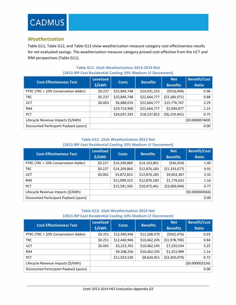
Utah 2013‐2014 HES Evaluation Appendix G5
Weatherization Table G11, Table G12, and Table G13 show weatherization measure category cost‐effectiveness results
for net evaluated savings. The weatherization measure category proved cost‐effective from the UCT and
RIM perspectives (Table G11).
Table G11. Utah Weatherization 2013‐2014 Net (2013 IRP East Residential Cooling 10% Medium LF Decrement)
Cost‐Effectiveness Test Levelized
$/kWh Costs Benefits
Net
Benefits
Benefit/Cost
Ratio
PTRC (TRC + 10% Conservation Adder) $0.237 $25,849,748 $24,931,255 ($918,494) 0.96
TRC $0.237 $25,849,748 $22,664,777 ($3,184,971) 0.88
UCT $0.063 $6,888,010 $22,664,777 $15,776,767 3.29
RIM $19,714,900 $22,664,777 $2,949,877 1.15
PCT $24,697,293 $18,537,852 ($6,159,441) 0.75
Lifecycle Revenue Impacts ($/kWh) ($0.000007469)
Discounted Participant Payback (years) 0.00
Table G12. Utah Weatherization 2013 Net (2013 IRP East Residential Cooling 10% Medium LF Decrement)
Cost‐Effectiveness Test Levelized
$/kWh Costs Benefits
Net
Benefits
Benefit/Cost
Ratio
PTRC (TRC + 10% Conservation Adder) $0.227 $14,209,860 $14,163,801 ($46,059) 1.00
TRC $0.227 $14,209,860 $12,876,183 ($1,333,677) 0.91
UCT $0.062 $3,872,815 $12,876,183 $9,003,367 3.32
RIM $11,099,552 $12,876,183 $1,776,631 1.16
PCT $13,541,505 $10,472,461 ($3,069,044) 0.77
Lifecycle Revenue Impacts ($/kWh) ($0.000004566)
Discounted Participant Payback (years) 0.00
Table G13. Utah Weatherization 2014 Net (2013 IRP East Residential Cooling 10% Medium LF Decrement)
Cost‐Effectiveness Test Levelized
$/kWh Costs Benefits
Net
Benefits
Benefit/Cost
Ratio
PTRC (TRC + 10% Conservation Adder) $0.251 $12,440,946 $11,508,470 ($932,476) 0.93
TRC $0.251 $12,440,946 $10,462,245 ($1,978,700) 0.84
UCT $0.065 $3,222,701 $10,462,245 $7,239,544 3.25
RIM $9,208,256 $10,462,245 $1,253,989 1.14
PCT $11,923,530 $8,620,451 ($3,303,079) 0.72
Lifecycle Revenue Impacts ($/kWh) ($0.000003156)
Discounted Participant Payback (years) 0.00
Utah 2013‐2014 HES Evaluation Appendix H1
Appendix H. HES Logic Model
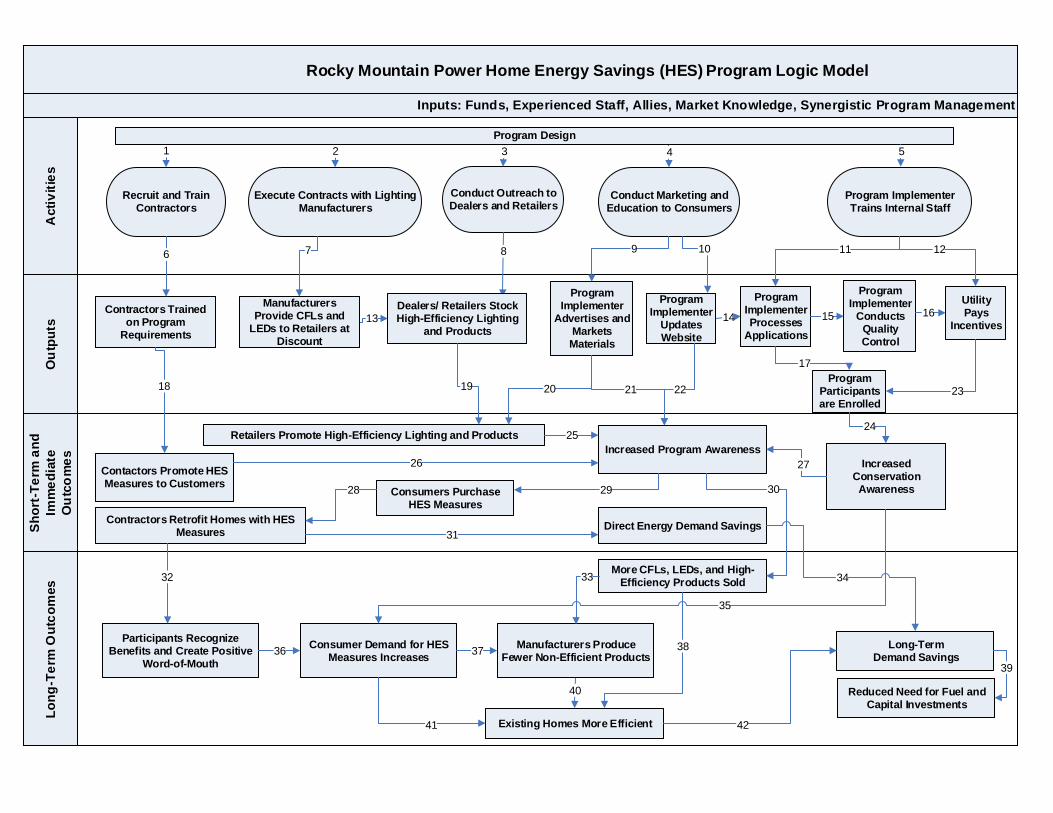
Rocky Mountain Power Home Energy Savings (HES) Program Logic Model
Lo
ng
-Te
rm O
utc
om
es
Sh
ort
-Te
rm a
nd
Imm
ed
iate
Ou
tco
me
s
Ou
tpu
tsA
cti
vit
ies
Inputs: Funds, Experienced Staff, Allies, Market Knowledge, Synergistic Program Management
Program Implementer Trains Internal Staff
Recruit and Train Contractors
Retailers Promote High-Efficiency Lighting and Products
Long-Term Demand Savings
Increased Conservation Awareness
Consumer Demand for HES Measures Increases
Participants Recognize Benefits and Create Positive
Word-of-Mouth
Conduct Outreach to Dealers and Retailers
More CFLs, LEDs, and High-Efficiency Products Sold
Direct Energy Demand Savings
Contractors Trained on Program
Requirements
Contactors Promote HES Measures to Customers
13 14
40
Execute Contracts with Lighting Manufacturers
36
Conduct Marketing and Education to Consumers
7 8 9
Manufacturers Provide CFLs and
LEDs to Retailers at Discount
Dealers/ Retailers Stock High-Efficiency Lighting
and Products
Program Implementer
Advertises and Markets Materials
10
Program Implementer
Updates Website
11 12
Program Implementer Processes
Applications
Utility Pays
Incentives
17
Program Participants are Enrolled
24
Contractors Retrofit Homes with HES Measures
Increased Program Awareness
37Manufacturers Produce
Fewer Non-Efficient Products
Reduced Need for Fuel and Capital Investments
Existing Homes More Efficient41
32
35
39
42
38
33 34
3029
31
18
26 27
25
2321 2219
6
1 2 3 4
Program Design
5
20
Program Implementer
Conducts Quality Control
15 16
Consumers Purchase HES Measures
28