Embed Size (px)
Citation preview

FInal Rep_CCEM.RF-K4.CL.doc Page 1 of 68
FINAL REPORT
CCEM.RF-K4.CL COMPARISON RF-Voltage measurements up to 1 GHz*
Jan P.M. de Vreede1
(Completed by James Randa2)
1 Department of Electricity, Radiation and Length Van Swinden Laboratorium
Thijsseweg 11, 2629 JA Delft, the Netherlands
2Electromagnetics Division National Institute of Standards and Technology
Boulder, CO 80305, U.S.A. e-mail: [email protected]
________________________________________________________________ * Partially supported by U.S. government work, not protected by U.S. copyright.

FInal Rep_CCEM.RF-K4.CL.doc Page 2 of 68
This comparison was initiated and led by Jan de Vreede, who sadly passed away during preparation of the final report. His friends and colleagues in
the comparison dedicate this report to his memory.

FInal Rep_CCEM.RF-K4.CL.doc Page 3 of 68
Abstract: We report the results of an international comparison of measurements of radio frequency voltage in the frequency range 1 MHz to 1 GHz. This comparison was performed as a “Key Comparison” under the auspices of the Consultative Committee for Electricity and Magnetism (CCEM) of the International Committee for Weights and Measures (CIPM). Participating laboratories were the designated National Metrology Institutes (NMIs) for their respective countries. Keywords: CCEM, GT-RF, international measurement comparison, radio frequency voltage Table of Contents 1 Introduction ........................................................................................................................ 4 2 Participants and schedule ................................................................................................... 4 3 Transfer standards and required measurements ................................................................. 7 4 Behaviour of the transfer standards ................................................................................... 7 5 Measurement methods ....................................................................................................... 8 6 Technical protocol ........................................................................................................... 11 7 Measurement results ........................................................................................................ 11
7.1 General results ......................................................................................................... 11 7.2 Determining reference values .................................................................................. 23
7.2.1 Thermal converter Ballantine ............................................................................ 23 7.2.2 Power sensor R&S ............................................................................................. 23 7.2.3 Check measurements ......................................................................................... 24
7.3 Values and uncertainties .......................................................................................... 25 7.3.1 Frequency: 1 MHz ............................................................................................. 26 7.3.2 Frequency 10 MHz ............................................................................................ 28 7.3.3 Frequency 50 MHz ............................................................................................ 30 7.3.4 Frequency 100 MHz .......................................................................................... 32 7.3.5 Frequency 200 MHz .......................................................................................... 34 7.3.6 Frequency 300 MHz .......................................................................................... 36 7.3.7 Frequency 500 MHz (optional) .......................................................................... 38 7.3.8 Frequency 700 MHz (optional) .......................................................................... 40 7.3.9 Frequency 1000 MHz (optional) ........................................................................ 42
7.4 Uncertainty budgets ................................................................................................. 44 8 Conclusions ...................................................................................................................... 44 9 Follow-up ......................................................................................................................... 44 10 References ........................................................................................................................ 44 Appendix A. Original Time Schedule ................................................................................. 45 Appendix B. Contact Persons .............................................................................................. 46 Appendix C. Technical Protocol .......................................................................................... 48 Appendix D. Submitted Results ........................................................................................... 59 Appendix E. Participants’ Uncertainty Budgets .................................................................. 63H68

FInal Rep_CCEM.RF-K4.CL.doc Page 4 of 68
1 Introduction During the nineteen eighties modern equipment in the field of ac-dc transfer and of ac-voltage came on the market operating up to tens of megahertz. Progress in microcircuits also led to the development of tools measuring voltages in the ranges up to 1 gigahertz. In 1992 the Working Group on Radio-Frequency Quantities (Groupe de Travail pour les grandeurs aux Radio-Fréquences, GT-RF) of the Comité Consultatif d’Electricité et Magnetism (CCEM) decided to start a comparison to investigate the quality of voltage measurements up to high frequencies of at least 300 MHz, with an optional frequency extension to 1 GHz. This comparison (GT-RF 92-6) is an extension of a similar proposal made in the 1992 CCEM meeting for a comparison on ac-dc transfer devices up to 50 MHz [1]. In order to avoid confusion it was decided to delay the start of the GT-RF comparison to such a time that the low-frequency CCEM comparison would almost be finished. After the introduction of the Mutual Recognition Arrangement (MRA) [2], the GT-RF comparison was assigned the number CCEM.RF-K4.CL. This report is the technical report on the complete exercise, including all the problems that occurred during the comparison. Already during the start of the project the role of comparisons as technical evidence of the performance of the national metrology institutes was indicated. Hence the pilot laboratory attempted to implement the expected requirements, e.g., a fixed measuring period, short reporting time and routine measurement conditions. It was not possible to decide on the method of calculating a reference value for the comparison and to obtain uncertainty budgets before the start of the comparison. In the CIPM guidelines [3] it is also suggested that a trial round will be held with a small group of laboratories and that they will perform an evaluation round. This trial round was carried out in 1997 between PTB (Germany), NRC (Canada) and the pilot laboratory VSL (the Netherlands), whose name was NMi-VSL when the comparison started. The full names of all participating national metrology institutes (NMIs) can be found in Table 1. In the past a similar intercomparison was organised under the umbrella of the GT-RF; viz. GT-RF 75-A5 [4] with PTB (Germany) as pilot. Due to the length of time it has taken to complete this comparison, and because of the disruption caused by Jan de Vreede’s untimely death and the consequent transfer of piloting responsibilities, the participants (with the approval of the CCEM) decided to complete the report under the old (pre-MRA) rules, which were in effect when the comparison began. Thus the final key comparison reference values (KCRVs) and degrees of equivalence (DOEs) were not computed and submitted to the Key Comparison Database (KCDB), and the comparison will be submitted for approval for provisional equivalence rather than full equivalence. However, since some work had been completed in computing KCRVs, we include those results in this report, calling them “reference values.” These results are reported in Section 7. Mention of trade names or specific products in this report does not indicate approval or disapproval of them by participants of the comparison. Specific companies and products are named only in order to provide adequate technical detail regarding the measurements.
2 Participants and schedule During 1996 invitations were sent out to participate in the comparison. Based upon the received information a time schedule and a transport scheme were determined. The comparison was split into 4 loops, two within the European Community and two outside it. In

FInal Rep_CCEM.RF-K4.CL.doc Page 5 of 68
this way an equal worldwide distribution was obtained, while still maintaining a relatively simple procedure for customs handling. However, almost immediately after the start of the first loop, damage to the equipment occurred. This led effectively to a restart of the comparison. The original time schedule is given in Appendix A, and the contact persons for the participating NMIs are listed in Appendix B. During the remainder of the comparison similar problems often occurred, which led to significant delays. Hence the pilot laboratory decided to make only short-term plans. The final time schedule is given in Table 1. Since RF-dc measurements are time consuming, due to their nature of measuring temperature differences and/or temperature stabilisation, each laboratory was allowed 5 weeks of measurements and one or two weeks of transport to the next participant. The ATA carnet was used outside the European Community (now European Union). Given VSL’s experience during this comparison, we now believe that a temporary import/export document within a star pattern comparison (return to the pilot laboratory after measurements at each laboratory) is preferred. The star pattern requires more work, but it has fewer long delays.
Table 1. List of participants and measurement dates.
Acronym
National Metrology Institute Country
Standard at the
laboratory
Date of submission of
report Comment
VSL Van Swinden Laboratorium
The Netherlands January 1997
Pilot Lab
NRC National Research Council Canada Canada March 1997 April 1998 Trial round
PTB Physikalisch-Technische
Bundesanstalt Germany April 1997
June 1997 Trial round
VSL METAS Switzerland -- Breakdown / ATA
VSL January 1998 SMU Slovak Insitute of
Metrology Slovak
Republic March 1998 June 1998
CMI Czech Metrological Institute
Czech Republic May 1998 June 1998 Withdrew before
Draft A was finished METAS Switzerland -- Problems with set-up;
no measurements VSL July 1998
Arepa AREPA Test & Calibration Denmark September
1998 February 1999
CEM Centro Espanol de Metrologia Spain October 1998 November
1998
INRIM (formerly
IEN)
Italy December 1998
February 1999 Breakdown of Ballantine; replaced.
Withdrew before Draft A was finished
BNM-
LCIE
Bureau National de Métrologie France February
1999
-- Breakdown of
Ballantine and R&S
VSL May 1999
Check measurement / Replacement of R&S
sensor

FInal Rep_CCEM.RF-K4.CL.doc Page 6 of 68
Acronym
National Metrology Institute Country
Standard at the
laboratory
Date of submission of
report Comment
SIQ Slovenian Institute for Quality Slovenia July / August
1999 February 2000
PTB Physikalisch-Technische
Bundesanstalt Germany August 1999
Intermediate check
NIST National Institute of Standards and Technology
United States of America
October 1999
December 1999
VSL December 1999
Check measurement
NMIA Australia April 2000
No results submitted due to withdrawal
after measurements KRISS Korean Research
Institute of Standards and Standardisation
Republic of Korea July 2000
March 2003 Breakdown of R&S / Repaired in KRISS
VSL December 2000
Check measurement
VNIIM Russian Federation January 2002 ?
VSL February 2002
Check measurement
NIM People’s Republic of
China March 2002
?
VSL April 2002 Check measurement PTB Physikalisch-
Technische Bundesanstalt
Germany May 2002 September
2003 Intermediate check
METAS Switzerland July 2002 September 2003
NMC (formerly SPRING)
Singapore
-- Breakdown of R&S
VSL August 2002
Check measurement / Replacement of R&S
sensor LNE
(formerlyBNM-LNE)
Laboratoire National de Métrologie et d’Essais
France October 2002
March 2004 New report submitted after discussion about
reference plane
VSL November 2002
NMC Singapore December 2002
March 2003
VSL February 2003

FInal Rep_CCEM.RF-K4.CL.doc Page 7 of 68
3 Transfer standards and required measurements
In order to evaluate the laboratory’s performance for RF voltage measurements in the frequency range up to 1 GHz the working group (GT-RF) decided to use both a device especially designed for RF-dc transfer difference and a normal power sensor, because either one of these instruments could be used to obtain traceability to the relevant SI unit, either via the low-frequency chain of ac-dc techniques or via a RF-power and RF-impedance chain. The two devices in the comparison were:
- a Ballantine model 1396A RF-dc transfer with the following characteristics: o Input voltage: 1,3 V o Output voltage: 7 mV (at nominal input voltage) o Input resistance: 200 Ω (nominal) o Output resistance: 7 Ω (nominal)
- a Rohde und Schwarz power sensor NRV-Z51 with the following characteristics: o Impedance: 50 ohms o Input power: -20 dBm to +20 dBm ( 0,01 mW to 100 mW) o Equivalent voltage: 22 mV to 2,2 V (visible by changing display parameter)
The Rohde und Schwarz sensor will be referred to as R&S. As ac-dc transfer devices (and therefore also RF-dc devices) are renowned for breaking down during interlaboratory comparisons, a check measurement was propose, which would exclude as much as possible the influence of the individual laboratory. The easiest check is a measurement of the two devices against each other, as all components are present in the package. Another check is either a DC voltage measurement or a 50 MHz measurement. The latter was not always carried out, and therefore no results are reported here. The participants were asked to submit measurement results on each device at 9 frequencies (six required frequencies: 1.0 MHz, 10 MHz, 50 MHz, 100 MHz, 200 MHz, and 300 MHz; and three optional frequencies: 500 MHz, 700 MHz, and 1 GHz) concerning its RF-dc transfer difference calibration factor together with an uncertainty (coverage factor k = 1). To substantiate the technical performance, the technical protocol put emphasis on the uncertainty statements and the consistency of the measurement results. Hence, a detailed uncertainty budget, containing sources and magnitudes, was requested, as well as the traceability of the standards, in order to take into account the possibility of correlation between the results from different laboratories. In principle this information is readily available, provided a laboratory operates effectively according to a quality assurance system based upon standards like ISO 17025.
4 Behaviour of the transfer standards Both types of transfer standards showed problems, but one broke down several times during the exercise. Therefore an identification scheme was defined to distinguish the different configurations during the exercise. In Table 2 an overview is given with the round identification. The rounds are groups of measurements on the same devices within a relatively short period. An asterisk in the table means that a suspicion of defect was indicated, but that the same device was used further on as no clear change could be detected. The main link between the results of the different laboratories is the continuous monitoring of the

FInal Rep_CCEM.RF-K4.CL.doc Page 8 of 68
DUTs during their stay at VSL. Two identical devices were kept at VSL especially for this purpose. These were characterised at the same time as the travelling standards in the normal traceability chain leading to the primary standards. After a breakdown of a travelling standard one of the monitoring devices was used to replace a damaged/repaired device. Different R&S sensors have been used, each of which broke down at least once. One sensor is identified by Z25, Z26 and Z27, and the other sensor by Z40 and Z41: after each breakdown the identifying code was modified. In the case of the Ballantine device 621, questions arose in measurements from December 1998 through February 1999, as indicated in Tables 1 and 2. Device 621 was temporarily replaced by device 239 at that time. However, it was established that 621 was operating properly, and 621 was used throughout the remainder of the comparison. The measurements on 239 were not used; the two participants who measured 239 either withdrew from the comparison or performed measurements on 621 at a later date. Thus the same Ballantine device was used throughout the comparison. Table 2: Devices used during the comparison.
Round Start Finish Ballantine device R&S device 1 End 1996 August 1997 621 Z40 2 September
1997 June 1998 621 Z25
3 September 1998
November 1998 621 Z25 *
3a December 1998
February 1999 239 Z25
4 July 1999 March 2000 621* Z25 5 August 2000 March 2001 621 Z26
6+7 July 2001 May 2002 621 Z41 8 August 2002 February 2003 621 Z27
5 Measurement methods The majority of the laboratories used a normal ac-dc system, often modified to allow measurements at high frequencies. There are some differences, especially concerning the connection of the Ballantine device to the measuring system. Already in the guidelines, it was mentioned that a potential problem for interpreting the data would be the choice of the measurement plane (or reference plane) to which the data are referred. Hence laboratories were asked to state their choice explicitly. For each laboratory the measurement procedure (including traceability) is briefly described here. VSL – pilot laboratory: At lower frequency (up to 100 MHz), the traceability is based on the calculable ac-dc transfer standard developed at VSL [5]. Above 1 MHz, the traceability is based on the RF-power traceability using thermistor mounts measured in the VSL microcalorimeter system and the reflection coefficients measured using a Vector Network Analyser (hp 8753E with test set hp 85044). During the comparison the results in the overlapping frequency range were used to obtain a smooth frequency response from low frequency to high frequency.

FInal Rep_CCEM.RF-K4.CL.doc Page 9 of 68
NRC: No measurements were done on the Ballantine system. The R&S sensor was measured against a working standard using an external Tee. The reference is the midplane of the Tee, a model UG-107B/U. During the measurements the same number of measurements were carried out for each of the two positions of the Tee. PTB: The RF voltage standard at PTB is a dry calorimeter. Its power traceability is based on the comparison with a thermistor mount calibrated in the PTB microcalorimeter, and its impedance traceability is based on ANA measurements referred to precision 7 mm air lines. Below 100 MHz the frequency-dependent power and impedance responses of this dry calorimeter were determined by extrapolation of the response at higher frequencies down to dc by modelling of the dry calorimeter. The dry calorimeter voltage standard has a type N-female connector and was connected directly to the Ballantine converter. For the R&S sensor the dry calorimeter connector was changed to a N-male connector and both devices were compared by means of a N-Tee. For the power sensor, the reference plane is the midpoint of a model UG-107B/U Tee. For the Ballantine converter, the reference plane is the midpoint of the built-in Tee of the converter. SMU: An ac-dc transfer system is used with a Fluke A55 (up to 50 MHz) and a thermistor mount hp 8478b as working standards. The thermistor mount was calibrated against the SMU thermistor voltage standard. As external Tee (for the R&S sensor) a General Radio 874-TL is used at lower frequencies and an Amphenol-Tuchel UG-107B/U at higher frequencies. The latter was of poor quality. CMI: A power splitter method is used with a resistive Tee and a levelling monitor in one arm. The working standard is an hp 8478b calibrated at PTB, Germany. The DC measurements are done separately. During the measurements the impedance of the R&S sensor changed. The results refer to the situation after the change. Arepa: An ac-dc transfer method is used with direct read-out. For the R&S sensor an external Tee is used. A Fluke 5800A is used at DC and 1 MHz. All other measurements are done using 1 MHz as intermediate reference. CEM: An ac-dc transfer system is used. Three different working standards have been used, viz. PTB Multijunction Thermal Converter (from 10 Hz to 1 MHz), a VSL Calculable HF device (1 MHz to 100 MHz) and a Ballantine 1396A thermal converter calibrated at NIST. Different lay-outs were used to connect the DUTs to the relevant working standards. INRIM: A basic RF-dc transfer system is used since the INRIM standard is a Ballantine 1396A, which is calibrated in-house against the INRIM primary standard, a power system. For the Ballantine, an external Tee is used to connect the two converters. In all other cases, the internal Tee of a Ballantine is used (either INRIM’s or the travelling standard).

FInal Rep_CCEM.RF-K4.CL.doc Page 10 of 68
SIQ: An ac-dc transfer system is used up to 20 MHz. For higher frequencies a two step approach is used by adding a RF-RF transfer to the lower frequency measurement. NIST: An RF-dc transfer system is used. For TVCs like the Ballantine 1396, the switch is connected to the internal Tee of the DUT. The other side of the Tee is connected via an airline and an attenuator to a thermistor mount. In the case of a device like the R&S sensor, an external Tee is used. The power readings are converted into voltage taking into account the relevant reflection coefficients. KRISS: An RF-dc transfer system is used with an NRV-Z51 sensor as voltage standard. The DUT’s are compared with the standard using a type N Tee or the built-in Tee with a type N f-f adapter. The RF-dc difference of the standard was determined from dc resistance, effective efficiency, and equivalent parallel conductance at the reference plane. The effective efficiency was measured using a direct comparison method against the standard thermistor mount, whose effective efficiency was measured with a Type-N microcalorimeter system. The admittance was measured with a precision LCR meter at 1 MHz, and with network analyzers at the other frequencies. The measured admittance was corrected for the ANA imperfections using standard air lines as the impedance standard. VNIIM: A direct comparison method is used, using a diode compensation voltmeter with diode measuring transducer, which was calibrated by the National AC Voltage Standard. A special T-joined (tee) type N-Tee connector was used to connect to the travelling standard. NIM: R&S NRV-Z51: In the frequency range (10 – 1000) MHz the output of the R&S sensor is kept constant by varying the output voltage of a generator, which output level is measured using the NIM primary voltage standard GDY69. The reference planes are about 3.2 mm apart. The dc value is measured parallel to the R&S read-out with a precision voltmeter 7081. At 1 MHz an ac-dc transfer method is used for comparing the R&S sensor with the NIM coaxial thermal voltage converter TRZ8202. Its built-in Tee is used as reference plane. Ballantine 1396A: The same ac-dc transfer method is used, but now the built-in Tee of the travelling standard is used. Check of DUTs: The Ballantine is used as reference: its voltage output is kept constant. The reference plane is the midplane of the built-in Tee. METAS: As laboratory standards, a TVC code HF6 (traceable to VSL) is used up to 50 MHz; up to 1000 MHz a R&S NRV-Z51 power sensor is used, which is characterised using a thermistor mount traceable to NPL. The measurement process is done in two steps using 1 kHz as intermediate between dc and the requested frequency. A Tee was always used to connect the DUT and reference to the generator. The midplane of the Tee used (external in case of the R&S sensor, internal in the other case(s)) is the reference plane for the results obtained. Afterwards a correction was applied for the VSWR of the devices. The VSWR was measured using a hp 8753D vector network analyser.

FInal Rep_CCEM.RF-K4.CL.doc Page 11 of 68
BNM-LNE: The normal ac-dc transfer method of BNM-LNE is used with some modifications for use at these higher frequencies (no measurements are carried out above 100 MHz). As a working standard, a Ballantine 1394 TVC is used. It was calibrated with a GR874-N adapter against a HF TVC constructed and calibrated at NMi-VSL. The same Tee as used in this calibration was used to obtain the measurement results. No direct measurements were done on the R&S sensor, only the requested check measurements. NMC: An ac-dc transfer system is used for the Ballantine 1396. A working standard is used as reference, calibrated at frequencies below 100 MHz to voltage standards (traceable to VSL) and above 100 MHz to power standards (microcalorimeter and thermistor mount), which are all maintained within NMC. For the R&S sensor the same method is used below 100 MHz, but at higher frequencies the DUT is measured against the working standard using a resistive splitter and a monitoring sensor at the other arm. 6 Technical protocol In the technical protocol (see Appendix C), participants were asked to present their measurement results in the format of the mean, including a statement of uncertainty with a coverage factor of k = 1 using a template sent together with the DUTs. In addition they were requested to give a detailed uncertainty budget that would allow the pilot laboratory to determine whether important contributions might have been overlooked and to allow for drafting a common agreed basis for uncertainty calculation in this field. Also the traceability for the standards used should be provided to insure that correlation between measurement results would not be overlooked. The problem of the reference plane was mentioned only in the main text. For the check measurement (measuring the two DUTs against each other) the definition of DUT and reference was explicitly asked. The protocol did not include any requirements concerning the ambient conditions. The comparison started before the official guidelines [3] were available. However, draft versions were available, and along with informal discussions they were used to define the technical protocol. Of course the global uncertainties given in the measurement reports were not modified. 7 Measurement results 7.1 General results
The participants were asked to submit measurement results on each device at 9 frequencies (6 required frequencies: 1.0 MHz, 10 MHz, 50 MHz, 100 MHz, 200 MHz and 300 MHz; 3 optional frequencies: 500 MHz, 700 MHz and 1000 MHz) concerning its RF-dc transfer difference calibration factor together with an extended uncertainty (coverage factor k =1). After receiving the measurement data (including uncertainty statement), the coordinator compiled these results in an Excel spreadsheet for further analysis. Each laboratory received the relevant part of this spreadsheet for checking the correctness of these data.

FInal Rep_CCEM.RF-K4.CL.doc Page 12 of 68
Figure 1 gives a general impression of the frequency response for the three measurands: the power sensor, the thermal converter, and the check measurement using the two devices against each other. One series of the pilot laboratory measurements is shown here as example. Especially for the thermal converter (Ballantine), large frequency deviations take
R&S Z51 (sn...25)
-5000
0
5000
10000
15000
20000
1 10 50 100 200 300 500 700 1000
Frequency (MHz)
RF-
DC
diff
eren
ce (p
pm)
Ballantine sn. 621
-200000
-150000
-100000
-50000
0
50000
100000
150000
200000
250000
1 10 50 100 200 300 500 700 1000
Frequency (MHz)
RF-
DC
diff
eren
ce (p
pm)
Ballantine sn. 621- R&S (..25)
-200000
-150000
-100000
-50000
0
50000
100000
150000
200000
250000
1 10 50 100 200 300 500 700 1000
Frequency (MHz)
RF-D
C di
ffere
nce
(ppm
)
Figure 1: Frequency response of the two devices and a check against each other (measurements performed at the pilot laboratory).

FInal Rep_CCEM.RF-K4.CL.doc Page 13 of 68
place, much larger than usually encountered on low frequency devices and high frequency power sensors. Figures 2 through 10 contain the results of the participants and the individual pilot measurements. The uncertainty bars refer to the (k=1) uncertainties as stated by the participants. The data submitted are summarized in Appendix D, and the uncertainty budgets of the participants are reported in Appendix E. During the analysis it became clear that indeed there was some confusion about the definition of the quantity to be reported: the largest differences between the results appeared to be due to opposite signs. The pilot has decided that its “own” sign convention is the correct one. Where relevant, the sign has been changed. As the thermal converter (Ballantine) was the only DUT that survived the entire exercise, a reference line representing an average of the pilot results is drawn in the figures for the Ballantine results to give an idea about the reproducibility or stability of the pilot measurements. For the power sensor (R&S) a total of 5 different devices have been used. The most obvious solution would be to look to the differences between the results obtained on the same device by a participant and the pilot. However, that would introduce the rather large pilot-lab uncertainties into all the power-sensor results. This point will be treated below, in Section 7.2.2. The check measurement (Ballantine directly against the R&S power sensor) should give consistent results, as one would only expect a statistical spread and no dependence on the traceability of the standards. Slight differences will occur because the same combination could not always be used.

FInal Rep_CCEM.RF-K4.CL.doc Page 14 of 68
Figure 2: The results obtained at 1 MHz by the participants for the three measurands. The results from the pilot laboratory are given as squares. The dotted lines indicate where a change in power sensor took place. The solid line in the Ballantine sensor graph is the average of the VSL results.

FInal Rep_CCEM.RF-K4.CL.doc Page 15 of 68
R&S sensor at 10 MHz
-0.80
-0.60
-0.40
-0.20
0.00
0.20
0.40
0.60
0.80
NR
C
PTB
-1
VS
L-1
VS
L-2
SM
U
VS
L-3
Are
pa
CE
MV
SL-
4
SIQ
PTB
-2
NIS
TV
SL-
5
KR
ISS
VS
L-6.
0V
SL-
6
VN
IIM
VS
L-7
NIM
VS
L-8
PTB
-3
ME
TAS
VS
L-9
BN
M-L
NE
VS
L-10
SP
RIN
G
VS
L-11
Lab
RF-
dc d
iffer
ence
(%)
Figure 3: The results obtained at 10 MHz by the participants for the three measurands. The results from the pilot laboratory are given as squares. The dotted lines indicate where a change in power sensor took place.

FInal Rep_CCEM.RF-K4.CL.doc Page 16 of 68
Figure 4: The results obtained at 50 MHz by the participants for the three measurands. The results from the pilot laboratory are given as squares. The dotted lines indicate where a change in power sensor took place.

FInal Rep_CCEM.RF-K4.CL.doc Page 17 of 68
Figure 5: The results obtained at 100 MHz by the participants for the three measurands. The results from the pilot laboratory are given as squares. The dotted lines indicate where a change in power sensor took place.

FInal Rep_CCEM.RF-K4.CL.doc Page 18 of 68
B allantine sensor at 200 MHz
-7.00
-6.00
-5.00
-4.00
-3.00
-2.00
-1.00
0.00
NR
C
PTB
-1
VS
L-1
VS
L-2
SM
U
VS
L-3
Are
pa
CE
M
VS
L-4
SIQ
PTB
-2
NIS
T
VS
L-5
KR
ISS
VS
L-6.
0
VS
L-6
VN
IIM
VS
L-7
NIM
VS
L-8
PTB
-3
ME
TAS
VS
L-9
BN
M-L
NE
VS
L-10
SP
RIN
G
VS
L-11
Lab
RF-
dc d
iffer
ence
(%)
Figure 6: The results obtained at 200 MHz by the participants for the three measurands. The results from the pilot laboratory are given as squares. The dotted lines indicate where a change in power sensor took place.
FInal Rep_CCEM.RF-K4.CL.doc Page 19 of 68
Figure 7: The results obtained at 300 MHz by the participants for the three measurands. The results from the pilot laboratory are given as squares. The dotted lines indicate where a change in power sensor took place.

FInal Rep_CCEM.RF-K4.CL.doc Page 20 of 68
Figure 8: The results obtained at 500 MHz by the participants for the three measurands. The results from the pilot laboratory are given as squares. The dotted lines indicate where a change in power sensor took place.

FInal Rep_CCEM.RF-K4.CL.doc Page 21 of 68
Ballantine sensor at 700 MHz
-16.00
-14.00
-12.00
-10.00
-8.00
-6.00
-4.00
-2.00
0.00
NR
C
PTB
-1V
SL-
1
VS
L-2
SM
UV
SL-
3
Are
paC
EM
VS
L-4
SIQ
PTB
-2N
IST
VS
L-5
KR
ISS
VS
L-6.
0
VS
L-6
VN
IIM
VS
L-7
NIM
VS
L-8
PTB
-3
ME
TAS
VS
L-9
BN
M-L
NE
VS
L-10
SP
RIN
G
VS
L-11
Lab
RF-
dc d
iffer
ence
(%)
Figure 9: The results obtained at 700 MHz by the participants for the three measurands. The results from the pilot laboratory are given as squares. The dotted lines indicate where a change in power sensor took place.

FInal Rep_CCEM.RF-K4.CL.doc Page 22 of 68
Ballantine sensor at 1000 MHz
0.00
5.00
10.00
15.00
20.00
25.00
NR
C
PTB
-1
VS
L-1
VS
L-2
SM
UV
SL-
3
Are
pa
CE
MV
SL-
4
SIQ
PTB
-2N
IST
VS
L-5
KR
ISS
VS
L-6.
0
VS
L-6
VN
IIM
VS
L-7
NIM
VS
L-8
PTB
-3
ME
TAS
VS
L-9
BN
M-L
NE
VS
L-10
SP
RIN
G
VS
L-11
Lab
RF-
dc d
iffer
ence
(%)
Figure 10: The results obtained at 1000 MHz by the participants for the three measurands. The results from the pilot laboratory are given as squares. The dotted lines indicate where a change in power sensor took place.

FInal Rep_CCEM.RF-K4.CL.doc Page 23 of 68
7.2 Determining reference values Because this comparison was begun under the “old rules,” before Key Comparison Reference Values (KCRVs) and Degrees of Equivalence (DOEs) were introduced and required, and because of problems arising from the transition to a new pilot laboratory, the participants and the CCEM agreed to complete the report under the old rules and to seek only provisional equivalence rather than full equivalence. Nevertheless, considerable work was done on computing reference values, and we therefore present those results. 7.2.1 Thermal converter Ballantine In this case, it would be possible to use the method of [6]. However, there was no provision in the protocol for identifying and excluding outliers. Therefore we use a simple mean of all measuremements as the reference value. The multiple results from the pilot are combined into one value and one uncertainty, and the same is done for the two official PTB results (PTB-1 and PTB-3). This is implemented in section 7.3. 7.2.2 Power sensor R&S There is a basic problem in treating the power-sensor results, due to the fact that the sensor had to be repaired and replaced several times during the course of the comparison, and therefore we must contend with the possibility that the different participants may have been measuring sensors with different characteristics. We are able to deal with this situation because the pilot lab (VSL) measured the sensor before and after each repair or replacement. One possible strategy would be to compute the differences between the results obtained on the same device by a participant and the pilot lab, thereby referencing all the results to the pilot lab’s measurements. There is, however, a significant problem with this procedure. The uncertainty in the difference between a participant’s result and the appropriate VSL result is the root sum of squares of the two individual uncertainties. But the uncertainties in many of the VSL results are quite large (cf. Figs. 2 – 10), and so in these cases the uncertainty in the difference will be dominated by the VSL uncertainty, and it will be so large as to obscure all but the most extreme disagreements. We therefore adopt a different strategy for dealing with potential changes in the power sensor. We observe that, although different sensors may in principle have different characteristics, in practice the RF-dc difference does not differ or change. This is seen by comparing the VSL measurements before and after each change in Figures 2 – 10. The RF-dc difference is very nearly the same before and after every change or repair at every frequency. Any small differences are comparable to the differences observed for the thermal converter (Ballantine) sensor, which was the same throughout the comparison. Therefore, since there is evidence that the different power sensors are very nearly the same (and no evidence of any significant difference), and since the alternative (subtracting the appropriate VSL measurement) washes out too much information, we choose to treat the power-sensor results as if all the power sensors are the same. The reference values are then computed in the usual manner, by taking the mean of the results from all the participants.

FInal Rep_CCEM.RF-K4.CL.doc Page 24 of 68
7.2.3 Check measurements In principle this measurement is not part of the comparison, but should give confidence in the stability of the devices and the individual measurement set-up. The results are summarized in Table 3 and Figure 11. In Table 3, the “Unc” (%) column is the larger of the average fractional uncertainty and the standard deviation of the fractional uncertainties, and the Max column is the larger of the two preceding columns. Table 3: Results of the check measurements divided in two groups (pilot and other participants)
Frequency Average (%) StDev (%) "Unc" (%) Max (%)
1 Others 0.01 0.04 0.03 0.04 VSL 0.00 0.12 0.23 0.23
10 Others -0.07 0.07 0.03 0.07 VSL -0.11 0.03 0.08 0.08
50 Others -0.33 0.11 0.09 0.11 VSL -0.42 0.08 0.08 0.08
100 Others -1.14 0.27 0.12 0.27 VSL -1.28 0.07 0.09 0.09
200 Others -4.07 0.86 0.13 0.86 VSL -4.46 0.18 0.10 0.18
300 Others -7.77 1.61 0.14 1.61 VSL -8.30 0.68 0.31 0.68
500 Others -13.55 2.58 0.25 2.58 VSL -14.18 1.31 0.18 1.31
700 Others -9.83 2.27 0.29 2.27 VSL -10.22 1.90 0.36 1.90
1000 Others 16.27 4.86 0.43 4.86 VSL 17.35 1.47 0.87 1.47

FInal Rep_CCEM.RF-K4.CL.doc Page 25 of 68
Figure 11: A summary of the check measurements in which the response of the thermal converter is measured against the response of the power sensor. Data are given in Table 3. The pink squares refer to VSL data. The diamonds refer to the average results from the other participants. The VSL data are offset in frequency, one bin to the right of the average results. 7.3 Values and uncertainties From the information on the RF-dc differences for the two DUTs, a reference value for each DUT is computed along the lines suggested above. There was no attempt to identify and exclude outliers. The reference value is based on the unweighted mean of all measurements and the associated standard uncertainty. These are indicated in the graphs of Figs. 12 – 20 as a bold line and two dashed lines (+ and – “limits”). The graphs and the accompanying tables (Tables 4 – 12) contain the measured values and uncertainties reported by the participants. The result of the pilot laboratory is an averaged value and is given as last of the list (all others are in chronological order). PTB acted a few times as an intermediate check, on request from the pilot laboratory, and therefore there are multiple PTB measurements. One of these measurements (PTB-2) was an informal check performed at the request of the pilot laboratory, and it is not included in the reference-value computation. The other two measurements (PTB-1 and PTB-3) were full measurements, and we have combined them into a single PTB result for inclusion in the reference-value computation. For each frequency an overview of the results is given by means of two figures and one table containing the data of the two DUTs. The data are presented in terms of percentage instead of using parts per million or just the unit. This choice leads to a reasonable presentation without too much change in the graphs and without too many insignificant digits.

FInal Rep_CCEM.RF-K4.CL.doc Page 26 of 68
7.3.1 Frequency: 1 MHz
Figure 12: Overview of the results obtained at a frequency of 1 MHz. The same data are given in Table 4. The bold line refers to the unweighted mean and the dashed lines indicate the k=1 lines.

FInal Rep_CCEM.RF-K4.CL.doc Page 27 of 68
Table 4: Results at 1 MHz.
Power sensor Thermal converter
Laboratory Value (%) Unc (k=1) Laboratory Value (%) Unc (k=1) NRC -0.028 0.002 PTB 0.002 0.015 PTB -0.002 0.010 SMU -0.006 0.036 SMU 0.001 0.030 Arepa -0.011 0.610 Arepa -0.004 0.610 CEM -0.009 0.005 CEM 0.017 0.004 SIQ -0.020 0.050 SIQ 0.020 0.046
NIST -0.033 0.035 NIST 0.002 0.035 KRISS -0.001 0.077 KRISS -0.008 0.077 VNIIM -0.002 0.003 VNIIM 0.001 0.001
NIM -0.020 0.014 NIM 0.004 0.009 METAS -0.001 0.115 METAS 0.005 0.115
BNM-LNE -0.003 0.002 SPRING 0.018 0.010 SPRING 0.007 0.011
VSL -0.016 0.380 VSL 0.029 0.374
Average -0.010 0.104 Average 0.005 0.102 Stdev. 0.014 0.183 Stdev. 0.011 0.183
In general there is a good agreement among the participants, although there are several cases in which pairs of laboratories differ by more than their stated uncertainties, and there are some laboratories that have significantly larger uncertainties. In the bottom row the first entry refers to the statistical spread in the values, whereas the second one refers to the statistical spread in the stated uncertainty.

FInal Rep_CCEM.RF-K4.CL.doc Page 28 of 68
7.3.2 Frequency 10 MHz
Figure 13: Overview of the results obtained at a frequency of 10 MHz. The same data are given in Table 5. The bold line refers to the unweighted mean and the dashed lines indicate the k=1 lines.

FInal Rep_CCEM.RF-K4.CL.doc Page 29 of 68
Table 5: Results at 10 MHz.
In general there is a good agreement among the participants, although there are several cases in which pairs of laboratories differ by more than their stated uncertainties, and there are some laboratories that have significantly larger uncertainties. In the bottom row the first entry refers to the statistical spread in the values, whereas the second one refers to the statistical spread in the stated uncertainty.
Power sensor Thermal converter Laboratory Value (%) Unc (k=1) Laboratory Value (%) Unc (k=1)
NRC -0.104 0.003 PTB -0.155 0.033 PTB -0.018 0.027 SMU -0.076 0.090 SMU -0.013 0.090 Arepa -0.165 0.610 Arepa 0.068 0.610 CEM -0.038 0.008 CEM 0.004 0.008 SIQ -0.080 0.065 SIQ 0.030 0.060
NIST -0.117 0.039 NIST 0.006 0.039 KRISS -0.139 0.120 KRISS 0.009 0.120 VNIIM -0.166 0.004 VNIIM 0.010 0.003
NIM -0.130 0.102 NIM 0.044 0.121 METAS -0.176 0.117 METAS -0.028 0.118
BNM-LNE -0.043 0.004 SPRING -0.139 0.020 SPRING -0.019 0.022
VSL -0.059 0.291 VSL -0.081 0.346
Average -0.119 0.116 Average -0.002 0.121 Stdev. 0.044 0.168 Stdev. 0.038 0.173
FInal Rep_CCEM.RF-K4.CL.doc Page 30 of 68
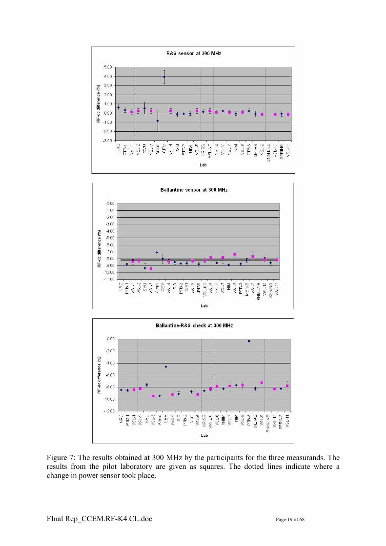
7.3.3 Frequency 50 MHz
Figure 14: Overview of the results obtained at a frequency of 50 MHz. The same data are given in Table 6. The bold line refers to the unweighted mean and the dashed lines indicate the k=1 lines.

FInal Rep_CCEM.RF-K4.CL.doc Page 31 of 68
Table 6: Results at 50 MHz.
In general there is a good agreement among the participants, although some have significantly larger uncertainties, and there is one pair of laboratories that differ by more than their stated uncertainties. In the bottom row the first entry refers to the statistical spread in the values, whereas the second one refers to the statistical spread in the stated uncertainty.
Power sensor Thermal converter Laboratory Value (%) Unc (k=1) Laboratory Value (%) Unc (k=1)
NRC -0.070 0.010 PTB -0.135 0.087 PTB -0.325 0.070 SMU -0.040 0.320 SMU -0.380 0.320 Arepa -0.268 0.610 Arepa -0.121 0.630 CEM 0.239 0.600 CEM -0.625 0.600 SIQ -0.060 0.100 SIQ -0.240 0.100
NIST -0.008 0.130 NIST -0.327 0.190 KRISS -0.094 0.123 KRISS -0.324 0.124 VNIIM -0.195 0.019 VNIIM -0.307 0.017
NIM -0.155 0.196 NIM -0.241 0.119 METAS -0.303 0.307 METAS -0.233 0.307
BNM-LNE -0.386 0.068 SPRING -0.134 0.050 SPRING -0.364 0.055
VSL -0.097 0.220 VSL -0.398 0.348
Average -0.102 0.213 Average -0.328 0.227 Stdev. 0.133 0.199 Stdev. 0.118 0.203

FInal Rep_CCEM.RF-K4.CL.doc Page 32 of 68
7.3.4 Frequency 100 MHz
Figure 15: Overview of the results obtained at a frequency of 100 MHz. The same data are given in Table 7. The bold line refers to the unweighted mean and the dashed lines indicate the k=1 lines.

FInal Rep_CCEM.RF-K4.CL.doc Page 33 of 68
Table 7: Results at 100 MHz.
Power sensor Thermal converter Laboratory Value (%) Unc (k=1) Laboratory Value (%) Unc (k=1)
NRC 0.040 0.031 PTB 0.012 0.163 PTB -1.295 0.130 SMU -0.110 0.490 SMU -0.250 0.540 Arepa -0.410 0.610 Arepa -0.560 0.630 CEM 0.910 0.620 CEM -1.842 0.620 SIQ 0.020 0.170 SIQ -1.180 0.190
NIST 0.067 0.150 NIST -1.259 0.210 KRISS -0.046 0.134 KRISS -1.267 0.136 VNIIM -0.129 0.057 VNIIM -1.160 0.057
NIM -0.184 0.196 NIM -1.160 0.126 METAS -0.329 0.307 METAS -0.955 0.307
BNM-LNE -0.835 0.256 SPRING -0.071 0.150 SPRING -1.298 0.155
VSL -0.042 0.218 VSL -1.209 0.352
Average -0.021 0.254 Average -1.098 0.285 Stdev. 0.313 0.197 Stdev. 0.389 0.195
In general there is a good agreement among the participants, although some have significantly larger uncertainties. The results from CEM show a relatively large deviation from the others. For SMU and Arepa the results show a much smaller deviation. In the bottom row the first entry refers to the statistical spread in the values, whereas the second one refers to the statistical spread in the stated uncertainty.

FInal Rep_CCEM.RF-K4.CL.doc Page 34 of 68
7.3.5 Frequency 200 MHz
Figure 16: Overview of the results obtained at a frequency of 200 MHz. The same data are given in Table 8. The bold line refers to the unweighted mean and the dashed lines indicate the k=1 lines.

FInal Rep_CCEM.RF-K4.CL.doc Page 35 of 68
Table 8: Results at 200 MHz.
Power sensor Thermal converter Laboratory Value (%) Unc (k=1) Laboratory Value (%) Unc (k=1)
NRC 0.297 0.127 PTB 0.103 0.220 PTB -4.580 0.150 SMU 0.140 0.510 SMU -4.750 0.590 Arepa -0.780 0.820 Arepa -3.010 0.870 CEM 3.296 0.640 CEM -5.539 0.640 SIQ 0.000 0.230 SIQ -4.400 0.290
NIST 0.130 0.200 NIST -4.580 0.230 KRISS 0.060 0.184 KRISS -4.580 0.194 VNIIM 0.157 0.087 VNIIM -4.556 0.087
NIM -0.117 0.191 NIM -4.541 0.149 METAS -0.187 0.307 METAS -4.162 0.307
BNM-LNE SPRING -0.137 0.280 SPRING -4.509 0.285
VSL 0.016 0.220 VSL -4.352 0.387
Average 0.229 0.309 Average -4.463 0.348 Stdev. 0.958 0.216 Stdev. 0.565 0.236
In general there is a good agreement among the participants, although some have significantly larger uncertainties. The results from CEM show a clear deviation from the others, while the Arepa results show a much smaller deviation. In the bottom row the first entry refers to the statistical spread in the values, whereas the second one refers to the statistical spread in the stated uncertainty.

FInal Rep_CCEM.RF-K4.CL.doc Page 36 of 68
7.3.6 Frequency 300 MHz
Figure 17: Overview of the results obtained at a frequency of 300 MHz. The same data are given in Table 9. The bold line refers to the unweighted mean and the dashed lines indicate the k=1 lines.

FInal Rep_CCEM.RF-K4.CL.doc Page 37 of 68
Table 9: Results at 300 MHz.
Power sensor Thermal converter Laboratory Value (%) Unc (k=1) Laboratory Value (%) Unc (k=1)
NRC 0.633 0.287 PTB 0.300 0.240 PTB -8.770 0.170 SMU 0.540 0.620 SMU -9.380 0.670 Arepa -0.820 1.100 Arepa -7.100 1.100 CEM 3.948 0.700 CEM -8.022 0.700 SIQ -0.100 0.230 SIQ -8.500 0.360
NIST -0.025 0.210 NIST -8.683 0.250 KRISS 0.169 0.232 KRISS -8.804 0.258 VNIIM 0.254 0.117 VNIIM -8.598 0.117
NIM -0.032 0.200 NIM -8.908 0.182 METAS -0.079 0.307 METAS -8.241 0.307
BNM-LNE SPRING -0.053 0.280 SPRING -8.602 0.300
VSL 0.107 0.224 VSL -8.164 0.690
Average 0.372 0.365 Average -8.481 0.425 Stdev. 1.131 0.277 Stdev. 0.566 0.297
In general there is a good agreement among the participants, although some have significantly larger uncertainties. The results from CEM show a clear deviation from the others, while the Arepa results show a much smaller deviation. This is especially the case for the power sensor. In the bottom row the first entry refers to the statistical spread in the values, whereas the second one refers to the statistical spread in the stated uncertainty.

FInal Rep_CCEM.RF-K4.CL.doc Page 38 of 68
7.3.7 Frequency 500 MHz (optional)
Figure 18: Overview of the results obtained at a frequency of 500 MHz. The same data are given in Table 10. The bold line refers to the unweighted mean and the dashed lines indicate the k=1 lines.

FInal Rep_CCEM.RF-K4.CL.doc Page 39 of 68
Table 10: Results at 500 MHz (optional frequency).
Power sensor Thermal converter Laboratory Value (%) Unc (k=1) Laboratory Value (%) Unc (k=1)
PTB 0.705 0.275 PTB -14.645 0.230 SMU 0.910 0.810 SMU -15.600 0.860 Arepa -0.960 1.100 Arepa -14.790 1.200 CEM CEM SIQ -0.480 0.330 SIQ -14.200 0.600
NIST -0.185 0.250 NIST -14.504 0.250 KRISS 0.395 0.316 KRISS -14.759 0.357 VNIIM 0.197 0.203 VNIIM -13.412 0.204
NIM 0.157 0.212 NIM -15.323 0.265 METAS 0.207 0.327 METAS -13.972 0.327
BNM-LNE SPRING 0.196 0.280 SPRING -14.337 0.300
VSL 0.417 0.252 VSL -13.864 0.982
Average 0.120 0.335 Average -14.491 0.507 Stdev. 0.483 0.301 Stdev. 0.636 0.231
CEM did not measure at this frequency. In general there is a good agreement between the participants. The Arepa result for the power sensor shows a somewhat large deviation. A few others show smaller deviations. For the thermal converter the uncertainty statements are quite small compared to the spread in the results. In the bottom row the first entry refers to the statistical spread in the values, whereas the second one refers to the statistical spread in the stated uncertainty.

FInal Rep_CCEM.RF-K4.CL.doc Page 40 of 68
7.3.8 Frequency 700 MHz (optional)
Figure 19: Overview of the results obtained at a frequency of 700 MHz. The same data are given in Table 11. The bold line refers to the unweighted mean and the dashed lines indicate the k=1 lines.

FInal Rep_CCEM.RF-K4.CL.doc Page 41 of 68
Table 11: Results at 700 MHz (optional frequency).
Power sensor Thermal converter Laboratory Value (%) Unc (k=1) Laboratory Value (%) Unc (k=1)
PTB 1.275 0.330 PTB -10.545 0.260 SMU 1.300 0.970 SMU -11.400 0.970 Arepa -1.400 1.100 Arepa -11.570 1.200 CEM CEM SIQ -0.890 0.380 SIQ -10.500 0.800
NIST -0.441 0.250 NIST -10.368 0.250 KRISS 0.615 0.377 KRISS -10.515 0.417 VNIIM -0.456 0.291 VNIIM -7.578 0.293
NIM 0.581 0.239 NIM -11.711 0.361 METAS 0.671 0.353 METAS -9.801 0.352
BNM-LNE SPRING 0.630 0.280 SPRING -10.017 0.300
VSL 0.870 0.255 VSL -9.578 1.610
Average 0.212 0.371 Average -10.326 0.619 Stdev. 0.827 0.320 Stdev. 1.150 0.461
CEM did not measure at this frequency. In general there is a wide spread in the results from the participants. The VNIIM result for the thermal converter shows a large deviation compared to its uncertainty. For the thermal converter the uncertainty statements are often quite small compared to the spread in the results. In the bottom row the first entry refers to the statistical spread in the values, whereas the second one refers to the statistical spread in the stated uncertainty.
FInal Rep_CCEM.RF-K4.CL.doc Page 42 of 68
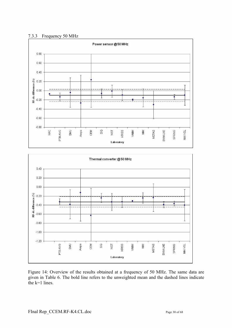
7.3.9 Frequency 1000 MHz (optional)
Figure 20: Overview of the results obtained at a frequency of 1000 MHz. The same data are given in Table 12. The bold line refers to the unweighted mean and the dashed lines indicate the k=1 lines.

FInal Rep_CCEM.RF-K4.CL.doc Page 43 of 68
Table 12: Results at 1000 MHz (optional frequency).
Power sensor Thermal converter Laboratory Value (%) Unc (k=1) Laboratory Value (%) Unc (k=1)
PTB 1.970 0.380 PTB 17.805 0.310 SMU 1.500 1.070 SMU 17.400 1.500 Arepa -1.820 1.200 Arepa 16.500 1.200 CEM -10.388 0.830 CEM 19.266 0.830 SIQ -1.510 0.440 SIQ 16.400 1.000
NIST -0.878 0.250 NIST 18.105 0.250 KRISS 1.047 0.435 KRISS 17.959 0.440 VNIIM 0.423 0.406 VNIIM 18.780 0.408
NIM 1.264 0.313 NIM 15.941 0.500 METAS 1.397 0.667 METAS 18.391 0.667
BNM-LNE SPRING 1.400 0.290 SPRING 17.823 0.320
VSL 1.404 0.298 VSL 17.964 1.614
Average -0.322 0.506 Average 17.695 0.753 Stdev. 3.264 0.343 Stdev. 0.988 0.476
In general there is a wide spread in the results from the participants compared to the stated uncertainties. This is influnced by the deviating value from CEM for the power sensor. For the thermal converter the uncertainty statements are often quite small compared to the spread in the results. In the bottom row the first entry refers to the statistical spread in the values, whereas the second one refers to the statistical spread in the stated uncertainty.

FInal Rep_CCEM.RF-K4.CL.doc Page 44 of 68
7.4 Uncertainty budgets All participants were requested to submit detailed uncertainty budgets for their measurements. The comparison protocol (Appendix C) included a form that could be used for this purpose, and most participants used this form or something similar. The uncertainty budgets of the participants are compiled in Appendix D. 8 Conclusions A long time has passed since the start of the comparison. Due to breakdown of devices and analysis problems at the pilot laboratory, a critical evaluation of the comparison is not simple. In general the stated uncertainties range from 100 ppm at low frequencies up to 0.3 % at 300 MHz and up to 0.5 % at the optional frequency of 1 GHz. Most results are in line with the stated uncertainties, but there are a number of cases in which pairs of laboratories differ by more than their stated uncertainties. The definition of RF-dc transfer warrants further discussion. 9 Follow-up It is not clear in what way a suitable follow-up can be carried out. A major problem is that many laboratories have indicated a reduced interest in this field.
10 References
[1] Final report on CCEM-K6c, Metrologia, 2005, 42, Tech. Suppl., 01002.
[2] Mutual Recognition of National Measurement Standards and of Calibration and Measurement Certificates Issued by National Metrology Institutes, endorsed by the International Committee on Weight and Measures, text available on the BIPM web site (www.bipm.org).
[3] Guidelines for CIPM key comparisons (www.bipm.org).
[4] GT-RF 75-A5: “Voltage (1 V) in 50 ohm coaxial line at 100, 250, 500 and 1000 MHz”, Metrologia, 20, 1984, pp.115-126
[5] C.J. van Mullem, W.J.G.D. Janssen and J.P.M. de Vreede, “Evaluation of the Calculable High Frequency AC-DC Standard”, IEEE Trans. Instrum.Meas., Vol. IM-46, April 1997, pp.361-364.
[6] J. Randa, "Proposal for KCRV & Degree of Equivalence for GTRF Key Comparisons", Document of the Working Group on radio frequency quantities of the CCEM, GT-RF/2000-12, September 2000.
[7] Guide to the Expression of Uncertainty in Measurement, ISO/TAG 4, published by ISO, 1993, corrected and reprinted 1995.
[8] EA document EA-04/02.

FInal Rep_CCEM.RF-K4.CL.doc Page 45 of 68
Appendix A. Original Time Schedule
Time schedule after stop at Swiss Telecom (September 1997)
Laboratory Contact Person Arrival date
SMU Ivan Petras 6 March 1998
CMI Frantisek Hejsek 10 April 1998
OFMET Peter Merki / Mark Flueli 15 May 1998
VSL Jan de Vreede 19 June 1998
Arepa Torsten Lippert 7 August 1998
CEM Miguel Neira 11 September 1998
IENGF Luciano Brunetti 16 October 1998
BNM-LCIE Luc Erard 20 November 1998
VSL Jan de Vreede 25 December 1998
SIQ Rado Lapuh 15 January 1999
NIST George Free
Joseph Kinard
19 February 1999
KRISS Jeong Hwan Kim 2 April 1999
CSIRO Joe Petranovic 7 May 1999
VSL Jan de Vreede 11 June 1999
VNIIM Dr. V.S. Alexandrow 2 July 1999
VSL Jan de Vreede 6 August 1999
FInal Rep_CCEM.RF-K4.CL.doc Page 46 of 68
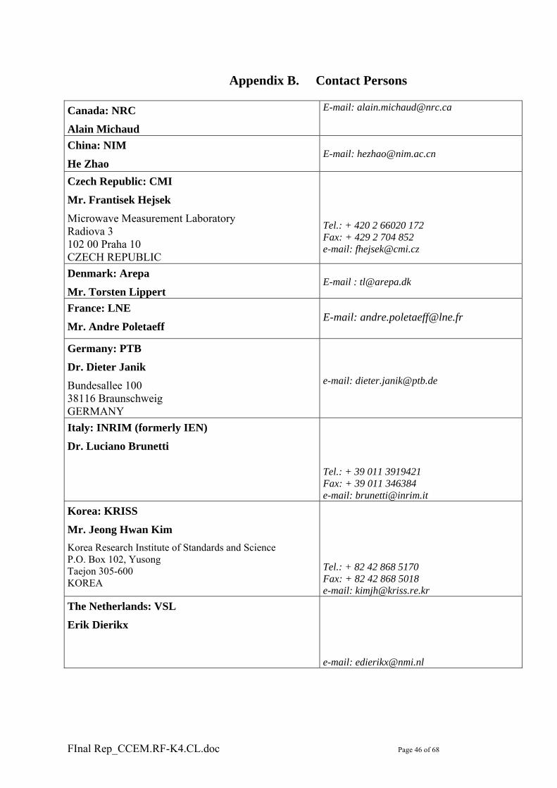
Appendix B. Contact Persons Canada: NRC
Alain Michaud
E-mail: [email protected]
China: NIM
He Zhao
E-mail: [email protected]
Czech Republic: CMI
Mr. Frantisek Hejsek Microwave Measurement Laboratory Radiova 3 102 00 Praha 10 CZECH REPUBLIC
Tel.: + 420 2 66020 172 Fax: + 429 2 704 852 e-mail: [email protected]
Denmark: Arepa
Mr. Torsten Lippert
E-mail : [email protected]
France: LNE
Mr. Andre Poletaeff
E-mail: [email protected]
Germany: PTB
Dr. Dieter Janik Bundesallee 100 38116 Braunschweig GERMANY
e-mail: [email protected]
Italy: INRIM (formerly IEN)
Dr. Luciano Brunetti
Tel.: + 39 011 3919421 Fax: + 39 011 346384 e-mail: [email protected]
Korea: KRISS
Mr. Jeong Hwan Kim Korea Research Institute of Standards and Science P.O. Box 102, Yusong Taejon 305-600 KOREA
Tel.: + 82 42 868 5170 Fax: + 82 42 868 5018 e-mail: [email protected]
The Netherlands: VSL
Erik Dierikx
e-mail: [email protected]

FInal Rep_CCEM.RF-K4.CL.doc Page 47 of 68
Singapore: NMC (formerly SPRING)
Dr Yueyan Shan Electromagnetic Metrology Department National Metrology Centre (NMC) Singapore 1 Science Park Drive, Singapore 118221 SINGAPORE
Tel: +65 – 6279 1929 Fax: +65 – 6279 1995 E-mail: [email protected]
Slovak Republic: SMU
Mr. Ivan Petráš Slovak Institute of Metrology Karloveská 63 842 55 Bratislava SLOVAKIA
Tel.: +421 7 60294243 Fax: +421 7 65429592 email: [email protected] [email protected]
Slovenia: SIQ
Mr. Rado Lapuh Metrology Department Tržaška cesta 2 1000 Ljubljana SLOVENIA
Tel.: +386 1 4770 300 Fax: +386 1 4778 303 email: [email protected]
Spain: CEM
Dr. Miguel Neira
E-mail: [email protected]
Switzerland: METAS (formerly OFMET)
Mr. Jurg Furrer EAM-HEV Lindenweg 50 CH-3003 Bern-Wabern SWITZERLAND
Tel.: + 41 31 323 3111 Fax: + 41 31 323 32 10 e-mail: [email protected]
USA: NIST
Joseph Kinard National Institute of Standards and Technology 100 Bureau Drive Mailstop 8171 Gaithersburg, MD 20899 USA
Tel.: (+1) 301-975-4250 e-mail: [email protected]
Russia: VNIIM
Dr. V. Telitchenko
E-mail: [email protected]

FInal Rep_CCEM.RF-K4.CL.doc Page 48 of 68
Appendix C. Technical Protocol
GT-RF comparison 92-6 CCEM.RF – K4b.CL
RF voltage measurements
at frequencies between 1 MHz and 1000 MHz
Technical Protocol
1. Scope During the last decades significant progress has been made in the development of AC calibration and measurement equipment. The equipment is now more user-friendly, can be operated by less qualified personel, but also generates signals to a higher frequency range where standard low frequency procedures might be no longer valid (with the small uncertainties associated with low-frequency measurements). One of the main parameters to be generated is AC voltage, but more appropiate above 1 MHz described as RF voltage. The scope of this comparison is to determine at which level worldwide traceability for the quantity RF Voltage (or RF/DC transfer) can be obtained. During the GT-RF meeting of September 2000 it was decided that the last loop of the GT-RF 92-6 should be separated from the earlier loops. Instead of the latter code CCEM.RF-K4.CL (or K4a.CL) its key comparison code is now CCEM.RF-K4b.CL. It is the intention that only one final report will be written covering both comparisons. 2. Definition of the measurand As indicated in the scope there is some ambiguity about the quantity to be measured. This is mainly due to the specific measurement set-up used and the frequency range. At low frequencies the usual measurement set-up will be an AC/DC transfer set-up with an (additional) DC voltage measurement if an absolute value of the AC voltage is required. The uncertainty in the latter measurement will most likely depend mainly on the long-term stability of the thermocouple output. For AC/DC transfer the relevant quantity is the AC/DC transfer difference, now more suitable called RF/DC transfer difference. The RF/DC transfer difference of a thermal converter (∗) is defined as:

FInal Rep_CCEM.RF-K4.CL.doc Page 49 of 68
dc
dcrf
VVV −
=δ
With Uth,rf=Uth,dc Where Vrf is the rms value of the applied RF voltage; Vdc is the mean value of the direct and reversed dc voltages, which produce the same output voltage Uth of the converter as Vrf At high frequencies the usual measurement set-up will be a determination of a calibration factor of a power sensor with a reference level at some high frequency, usually 50 MHz. In this way an absolute power level is obtained. The voltage level is then calculated using a nominal or measured impedance value. The relevant quantity here is voltage (absolute), but can be converted to a similar quantity as above (relative difference). Neglecting loading problems of the signal generator, it is, however, possible to use these systems also the other way around. Therefore we have decided on a set of transfer standards which can be used in both these types of measurement set-up. 3. The travelling standards Two devices are used as travelling standards. As indicated below they are based upon different design: - A Ballantine 1396A thermal converter - A Rohde und Schwarz power meter NRVD with power sensor NRV-Z51. For each device a short description is given below. 1) thermal converter A commercial (Ballantine model 1396A) thermal converter is used as representative of RF/DC thermal transfer devices. In contrast to the normal type of converters the device is equipped with a built-in Tee at its input connector (type-N male) and has a type-N male signal output (apparently meant to be terminated in a 50 Ω system). The thermal detector output is an MS 3102A-105L-3P connector. An adapter to banana connectors is supplied. The main specifications are: Input voltage: 1,3 V Output voltage: 7 mV (at nominal input voltage) Input resistance: 200 Ω (nominal) Output resistance: 7 Ω (nominal) The reference plane is at the midplane of the built-in Tee. Using the requested input voltage of 1,0 V an output of about 4 mV is to be expected when terminated with 50 Ω. Please remember that there will be a significant change in applied voltage if a 50 Ω termination is removed from the measurement set-up: therefore a blow-up of the converter is very likely.

FInal Rep_CCEM.RF-K4.CL.doc Page 50 of 68
2) Power meter with sensor In contrast to most high frequency power sensors the R&S power sensor NRV-Z51 has its lower frequency limit at DC. Therefore, together with its read-out unit NRVD, it can also be considered to be a RF/DC transfer with built-in display: hence acting as a RF voltmeter. The standard is equipped with a male type-N connector. The meter can be controlled via IEEE-488 interface. Manuals and the relevant IEEE-commando’s are also provided (see page 7/9). The main specifications are: Impedance: 50 ohms Input power: -20 dBm to +20 dBm ( 0,01 mW to 100 mW)
equivalent voltage: 22 mV to 2,2 V (visible by changing display parameter) 3.1 Quantity to be measured As indicated before, care has to be taken about what really is being measured. Hence we suggest the following approach for measuring the NRVD-system. If during the measuring process the voltage reading of the NRVD system is kept constant (i.e. the same voltage reading at the NRVD display), the system can be considered to act as a thermal converter: one has to compare the RF voltage at the input connector of the NRVD (or in the center of the T: please, specify your choice) with the DC voltage giving the same indication (voltage) at the NRVD display. In this case there is no need to calibrate the NRVD before, nor you have to use the 50 MHz source. If no RF voltage standard is available, the NRVD can be calibrated by determining the calibration factor and measuring the input impedance at RF and DC. Note, when measuring the combination of the Ballantine and the NRVD-system (section 5.2), the output of the Ballantine should be kept constant. Its output is much more frequency dependent. 4. Measuring conditions The participating laboratories are asked to follow their usual measurement procedure to their best measurement capabilities in respect to the allowed time frame (1 month) for the comparison. Hence, the measurand (RF/DC transfer or RF voltage) might be determined directly or in a two-step process using an intermediate frequency of e.g. 1 kHz. Note: It has been suggested that more reproducable results are obtained if the DUT and reference connections to the Tee are exchanged and averaged. This is, of course, not possible when using the Ballantine only. Important points to be mentioned in the report are: - The reference plane for the calibration

FInal Rep_CCEM.RF-K4.CL.doc Page 51 of 68
- Where relevant, the input and the output of the transfer devices have to be earthed in order to protect the insulation between the heater and the thermocouple.
- the accuracy and stability of the frequency (the measuring frequency has a significant influence on the RF/DC transfer)
- Is the final result due to an average using an exchange of the Tee-connections? 5. Measuring scheme 1) Calibration of the separate travelling standards The requested measurand has to be measured at the prescribed voltage (nominal 1 V), if possible. The measurement frequencies are given in the table below with six required frequencies and the other three are optional.
fmeas (MHz) 1
10
50
100 200 300
Optional (MHz)
500
700
1000
The requested measurand is the RF/DC transfer difference for the Ballantine, and the RF/DC voltage difference for the NRV-system (the latter might be converted into a RF/DC transfer difference: please, make clear which option is used). 2) Calibration of the two travelling standards against each other (if possible) A measurement at the six frequencies (1, 10, 50, 100, 200 and 300 MHz) is required of both travelling standards at the nominal input voltage of 1 V. For this purpose a female-female adapter is provided together with an insertion ring. This ring should be inserted in the adapter at the connector interface with the Ballantine (on the adapter is indicated in which connector the ring has to be inserted). In this case the relation between the two measurands (i.e. the RF/DC difference of the Ballantine using constant output voltage of the Ballantine) should be reported. 3) Additional check measurements To keep track of the performance of the devices we ask you to carry out, at least once, the following check measurements, if possible: - output of Ballantine using exactly 1,00.. V DC-input (while terminated in 50 Σ) - output of NRV-system using exactly 1,00.. V DC-input - output of NRV-system using the 50 MHz reference output - input impedance of NRV-Z51 sensor at the frequencies used. 6. Uncertainty statements The measurements should be performed at the lowest possible uncertainty level. A detailed uncertainty analysis for the measurements has to be reported in accordance with the GUIDE TO EXPRESSION OF UNCERTAINTY IN MEASUREMENT, first published in 1993 by BIPM/IEC/IFCC/ ISO/IUPAP/OIML, based on the RECOMMENDATION INC-1 (1980) of

FInal Rep_CCEM.RF-K4.CL.doc Page 52 of 68
the working group and the CIPM on the Statement of Uncertainties, English version published in Metrologia 17 (1981), p. 73. Participants are asked to assign Type A and B evaluation of the uncertainties mentioned, and to report sources and values separately. At the end the standard measurement uncertainty should be stated. All uncertainties should be given at a confidence level of 68% (1Φ or k=1 in present nomenclature). Also the degrees of freedom for each source of uncertainty should be given. 7. Report After carrying out the measurements, each participating laboratory should send a report to the pilot laboratory within 6 weeks including the form ‘Results of GT-RF 92-6 Comparison’. Short response time is necessary to check the status of the standards and to finish the comparison in the shortest time frame possible. The report should contain at least: - A detailed description of the measurement set-up including some drawings, which can be
used in the final report and a publication of the results; - A detailed description of the measurement procedure; - The mean measurement value and the statistical spread of the measurands of the standards
for each frequency measured, together with the number of measurements to produce this mean value;
- A detailed uncertainty budget in accordance with the GUIDE TO EXPRESSION OF UNCERTAINTY IN MEASUREMENT, first published in 1993 by BIPM/IEC/IFCC/ ISO/IUPAP/OIML. See also the form ‘Uncertainty budget of the GT-RF 92-6 comparison’, which is attached to this instruction set;
- The form ‘Results of GT-RF 92-6 Comparison’. The report should be sent as a hardcopy by mail. It would be appreciated if an electronic version would be sent by e-mail (preferably with the same lay-out as proposed in this instruction set). However, in case of problems the hardcopy version will be considered to be the official one. 8. Transportation and customs The devices should be (hand-) carried by car, train or plane as it appears the safest for the devices. The devices are stored as one package. This case is provided by the pilot laboratory ! Changing or deleting this case should be reported immediately to the pilot laboratory, with explanation. Each laboratory is responsible for the devices from the receipt of the DUTs until arrival of the DUTs at the next laboratory: this means it should cover the costs, if damages occur during the stay at the laboratory and the following transport. Inside the European Union no custom papers are necessary. For all the participants outside the European Union, an ATA-carnet will be provided, if applicable.

FInal Rep_CCEM.RF-K4.CL.doc Page 53 of 68
If your country accepts this document for temporary import, make sure that the document is used in the proper way both during entry and during exit (each time it should be submitted to customs!!). The ATA document should not be put inside the package. The contents of the package is given at the end of the instructions set (page 7). 9. Circulation time schedule After the trial loop (participants: VSL, NRC and PTB) at the beginning of 1997 the CCEM.RF-K4.CL has started started in October 1997. Unfortunately problems with the ATA-carnet and damage to equipment occurred. It is restarted at the beginning of March 1998 and was expected to finish sometime in 1999. Due to additional problems the final measurements of CCEM.RF-K4a.CL have been done at the end of 2000. In this part of the comparison the following laboratories participated: NIST (USA), KRISS (South Korea), CSIRO-NML (Australia), IENGF (Italy), SMU (Slovakia), CMI (Czechia) and VSL. In the CCEM.RF-K4b.CL comparison the following laboratories are participating: VNIIM (Russia), BNM-LNE (France), NIM (China), PSB (Singapore) and METAS (Switzerland). Intermediate checks will be carried out at VSL and PTB. The time allotted for each laboratory is 5 weeks (incl.transport). Updates of the schedule will be given to the participants as soon as possible. 10. Organisation The pilot laboratory for the comparison is the NMi Van Swinden Laboratorium (VSL). Each participant will receive information about the next participant as soon as possible. It is the responsibility of the participating laboratory to inform the next participant in advance to arrange the transportation of the standards to him, and to inform the pilot laboratory about the date of transportation (see forms on pages 10 and 11). 11. Contact person If there are any questions concerning the comparison, the contact person at the pilot laboratory is: Dr. Jan P.M. de Vreede NMi Van Swinden Laboratorium Schoemakerstraat 97 P.O. Box 654 2600 AR Delft ,The Netherlands Telephone: + 31-15 269 15 00 Telefax: + 31-15 261 29 71 E-mail: [email protected] =====================================================

FInal Rep_CCEM.RF-K4.CL.doc Page 54 of 68
Contents of package for GT-RF 92-6 1: Ballantine RF/dc transfer converter: Model 1396 A-1-10 sn: 621 2: Rohde und Schwarz display unit: Model NRVD sn: 841234 / 024 3: Rohde und Schwarz power sensor: Model NRV-Z51 sn: 837895 / 040 (sticker Z41) 4: MS-banana adapter for Ballantine converter 5: Suhner adapter type-N Model 31 N-50-0-51 (female - female) 6: insertion ring (provided by PTB; slightly damaged due to use) 7: manual for Ballantine 1396A 8: manual for Rohde und Schwarz NRVD 9: manual for Rohde und Schwarz NRV-Z51 Note: Items 5 and 6 are mounted in item 1 (for safety purposes). A single bended piece of wire is provided (in the same package) for removal and insertion of item 6 into item 5. Additional information concerning use of NRV-system - The sensor NRV-Z51 should be inserted in the interface slot A (the cable should be on the
left side of the slot). - Read-out of the instrument is only possible by IEEE-commands or by eye ! - The following set-up has to be used:
- NRVD to voltage read-out: press knobs: <Unit> and <V> - NRVD in high resolution mode: press knobs: <displ>, <resol> and <high> - NRVD in SCPI mode: press knobs: <spec>, <more> (4 times), <LNG> and
<SCPI> - relevant IEEE-commands (in SCPI-mode) (“IEEE-command”):
- read-out voltage: “*trg”

FInal Rep_CCEM.RF-K4.CL.doc Page 55 of 68
Results of GT-RF 92-6 Comparison On this form, the participant is kindly requested to present an overview of the results of his/her measurements on the travelling standards: the number of measurements (# meas.), the average of the measurand (V or ∗) and the corresponding total uncertainty (Φt) expressed as a 1Φ value. (It can be handwritten.) Institute: Date: Remarks: Travelling standard: Ballantine
frequency (MHz)
1
10 50 100 200 300 500 (optional)
700 (optional)
1000 (optional)
# meas.
∗ (ppm)
Φt (ppm)
Travelling standard: NRV-Z51
frequency (MHz)
1
10 50 100 200 300 500 (optional)
700 (optional)
1000 (optional)
# meas.
∗V (ppm)
Φt (ppm)
Also, the measurement results of the Ballantine versus the NRV-Z51 can be put on this form with: ∗ is the measured ∗ DUT-∗ REF; Φm is the standard deviation of the measurements. Travelling standards: Ballantine versus NRV-Z51 REFERENCE: ............... DUT: ...............
frequency (MHz)
1
10 50 100 200 300 500 (optional)
700 (optional)
1000 (optional)
# meas.
∗ (ppm)
Φt (ppm)

FInal Rep_CCEM.RF-K4.CL.doc 56/68
Uncertainty budget of the GT-RF 92-6 comparison This form can be used as an example to determine and to express the uncertainty of the measurements. It can be filled in (handwritten) or put in an appendix of your report on a form like this one. You can add your own sources of uncertainty, this is just an example. Our main goal is to have an uniform presentation of the uncertainty budget and corresponding an easy comparison between the results of the different institutes. Thank you in advance for your cooperation. Institute: Date: Remarks: Travelling standard: Ballantine Contribution of: Unc.
f: MHz Unc.
f: MHzUnc.
f: MHzUnc.
f: MHzType A
or B Shape of
distribution st. dev. of measurement
reference standard
measurement set-up
connectors
..........
..........
..........
total uncertainty (1Φ):
Travelling standard: NRV-Z51
Contribution of: Unc.
f: MHz Unc.
f: MHzUnc.
f: MHzUnc.
f: MHzType A
or B Shape of
distribution st. dev. of measurement
reference standard
measurement set-up
connectors
..........
..........
..........
total uncertainty (1Φ):

FInal Rep_CCEM.RF-K4.CL.doc 57/68
Notice of receipt of the GT-RF 92-6 package
To be sent to the pilot laboratory and to the next laboratory in the schedule Laboratory : Contact person : Herewith we inform you that we have received the package on: ……………………………….. Arrival of the ATA-carnet with the package: yes / no Remarks concerning the package itself : Remarks concerning the devices: Expected date of finishing the measurements of the devices:…………………. Expected date of dispatch of the devices to the next laboratory:…………………………… =======================================================================

FInal Rep_CCEM.RF-K4.CL.doc 58/68
Notice of dispatch of the GT-RF 92-6 package
To be sent to the pilot laboratory and to the next laboratory in the schedule Laboratory : Contact person : Herewith we inform you that we have dispatched the package on: ……………..………to the next participant :………………………………. We have checked that the ATA-carnet is sent with the package (but not inside the package): yes / no (Note: see the instruction set!!) Remarks concerning the package itself : Remarks concerning the devices:

FInal Rep_CCEM.RF-K4.CL.doc 59/68
Appendix D. Submitted Results NRC
f(MHz) NRVZ51 delta
u(k=1) Ballantinedelta
u(k=1) Check delta
u(k=1)
1 -281 21 240
10 -1043 34 1070
50 -697 98 3800
100 399 312 12300
200 2974 1270 43800
300 6326 2872 84500
500 141000
700 99000
1000 -179000
PTB-1
f(MHz) NRVZ51 delta
u(k=1) Ballantinedelta
u(k=1) Check delta
u(k=1)
1 -70 150 10 100 -100 120
10 -1400 330 130 270 -1430 300
50 -800 870 3200 700 -3800 750
100 300 1630 12900 1300 -12300 1400
200 2000 2200 45900 1500 -43800 1700
300 3500 2400 87900 1700 -84900 1900
500 6700 2750 147200 2300 -141700 2500
700 11200 3300 105700 2600 -100000 2800
1000 15800 3800 -178300 3100 179400 3300

FInal Rep_CCEM.RF-K4.CL.doc 60/68
VSL-1 f(MHz) NRVZ51
delta u(k=1) Ballantine
delta u(k=1) Check
delta Std. Dev.
1 338 3550 -24 3002 -27 120
10 -1011 2900 -1068 3015 -1074 300
50 -844 2700 -3566 3092 -3572 750
100 -271 2700 -11995 3311 -11993 1400
200 684 2700 -43379 3448 -43365 1700
300 1205 2700 -84243 3551 -84214 1900
500 3702 2950 -141159 3905 -141104 2500
700 7455 3000 -99088 4104 -99034 2800
1000 12106 3650 179570 4460 179537 3300
VSL-2
f(MHz) NRVZ51 delta
u(k=1) Ballantinedelta
u(k=1) Check delta
Std. Dev.
1 -267 3550 -38 3002 -41 120
10 -591 2950 -1090 3015 -1096 300
50 -636 2750 -3051 3092 -3057 750
100 89 2700 -11109 3311 -11107 1400
200 1118 2700 -42138 3448 -42124 1700
300 2541 2750 -82316 3551 -82287 1900
500 6372 2950 -137357 3905 -137302 2500
700 10983 3000 -95659 4104 -95605 2800
1000 15355 3100 179912 4460 179879 3300
SMU
f(MHz) NRVZ51 delta
u(k=1) Ballantinedelta
u(k=1) Check delta
u(k=1)
1 -60 360 -10 300 70 200
10 -760 900 130 900 -820 400
50 -400 3200 3800 3200 -3200 1000
100 -1100 4900 2500 5400 -11000 3000
200 1400 5100 47500 5900 -41000 3000
300 5400 6200 93800 6700 -76000 3000
500 9100 8100 156000 8600 -122000 6000
700 13000 9700 114000 9700 -88000 6000
1000 15000 10700 -174000 15000 228000 12000

FInal Rep_CCEM.RF-K4.CL.doc 61/68
VSL-3
f(MHz) NRVZ51 delta
u(k=1) Ballantinedelta
u(k=1) Check delta
Std. Dev.
1 -267 3550 155 3002 152 120
10 -591 2950 -820 3015 -826 300
50 -636 2750 -3831 3092 -3837 750
100 89 2700 -13349 3311 -13347 1400
200 1118 2700 -48481 3448 -48467 1700
300 2541 2750 -94564 3551 -94535 1900
500 6372 2950 -166100 3905 -166045 2500
700 10983 3000 -135094 4104 -135040 2800
1000 15355 3100 151191 4460 151158 3300
Arepa
f(MHz) NRVZ51 delta
u(k=1) Ballantinedelta
u(k=1) Check delta
u(k=1)
1 -110 6100 40 6100 130 50
10 -1650 6100 -680 6100 910 50
50 -2680 6100 1210 6300 3740 30
100 -4100 6100 5600 6300 13200 300
200 -7800 8200 30100 8700 48100 400
300 -8200 11000 71000 11000 94200 600
500 -9600 11000 147900 12000 165900 1000
700 -14000 11000 115700 12000 135400 1000
1000 -18200 12000 -165000 12000 -149800 900
CEM
f(MHz) NRVZ51 delta
u(k=1) Ballantinedelta
u(k=1) Check delta
Std. Dev.
1 -87 47 -173 44 -32 22
10 -375 82 -40 82 -354 15
50 2388 6000 6250 6000 -1561 27
100 9100 6200 18420 6200 -6263 18
200 32961 6400 55391 6400 -23135 10
300 39479 7000 80219 7000 -45988 18
500
700
1000 -103880 8300 -192660 8300 77235 21

FInal Rep_CCEM.RF-K4.CL.doc 62/68
VSL-4
f(MHz) NRVZ51 delta
u(k=1) Ballantinedelta
u(k=1) Check delta
Std. Dev.
1 -267 3550 -309 3079 -1615 16753
10 -591 2950 -108 3132 -840 165
50 -636 2750 -2980 3001 -3059 266
100 89 2700 -11648 3000 -12254 847
200 1118 2700 -42742 3118 -47068 820
300 2541 2750 -83886 3098 -92221 362
500 6372 2950 -141939 3000 -161843 301
700 10983 3000 -100174 3110 -130453 451
1000 15355 3100 181338 3006 153749 613
SIQ
f(MHz) NRVZ51 delta
u(k=1) Ballantinedelta
u(k=1) Check delta
u(k=1)
1 -200 500 -200 460 -200 440
10 -800 650 -300 600 0 600
50 -600 1000 2400 1000 2900 1000
100 200 1700 11800 1900 12700 1900
200 0 2300 44000 2900 47000 2900
300 -1000 2300 85000 3600 91000 3600
500 -4800 3300 142000 6000 156000 6000
700 -8900 3800 105000 8000 124000 8000
1000 -15100 4400 -164000 10000 -164000 10000
NIST
f(MHz) NRVZ51 delta
u(k=1) Ballantinedelta
u(k=1) Check delta
u(k=1)
1 -333 350 -15 350 -53 480
10 -1169 390 -56 390 -130 510
50 -75 1300 3272 1900 3474 220
100 666 1500 12591 2100 13154 2300
200 1304 2000 45801 2300 46445 2700
300 -251 2100 86831 2500 87246 2900
500 -1849 2500 145042 2500 145520 3190
700 -4406 2500 103677 2500 104392 3450
1000 -181048 2500 -181048 2500 -181884 3500
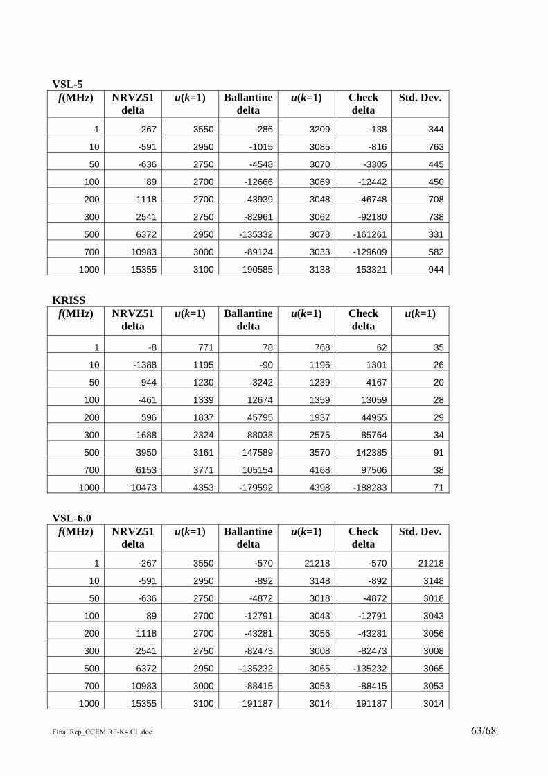
FInal Rep_CCEM.RF-K4.CL.doc 63/68
VSL-5
f(MHz) NRVZ51 delta
u(k=1) Ballantinedelta
u(k=1) Check delta
Std. Dev.
1 -267 3550 286 3209 -138 344
10 -591 2950 -1015 3085 -816 763
50 -636 2750 -4548 3070 -3305 445
100 89 2700 -12666 3069 -12442 450
200 1118 2700 -43939 3048 -46748 708
300 2541 2750 -82961 3062 -92180 738
500 6372 2950 -135332 3078 -161261 331
700 10983 3000 -89124 3033 -129609 582
1000 15355 3100 190585 3138 153321 944
KRISS
f(MHz) NRVZ51 delta
u(k=1) Ballantinedelta
u(k=1) Check delta
u(k=1)
1 -8 771 78 768 62 35
10 -1388 1195 -90 1196 1301 26
50 -944 1230 3242 1239 4167 20
100 -461 1339 12674 1359 13059 28
200 596 1837 45795 1937 44955 29
300 1688 2324 88038 2575 85764 34
500 3950 3161 147589 3570 142385 91
700 6153 3771 105154 4168 97506 38
1000 10473 4353 -179592 4398 -188283 71
VSL-6.0
f(MHz) NRVZ51 delta
u(k=1) Ballantinedelta
u(k=1) Check delta
Std. Dev.
1 -267 3550 -570 21218 -570 21218
10 -591 2950 -892 3148 -892 3148
50 -636 2750 -4872 3018 -4872 3018
100 89 2700 -12791 3043 -12791 3043
200 1118 2700 -43281 3056 -43281 3056
300 2541 2750 -82473 3008 -82473 3008
500 6372 2950 -135232 3065 -135232 3065
700 10983 3000 -88415 3053 -88415 3053
1000 15355 3100 191187 3014 191187 3014

FInal Rep_CCEM.RF-K4.CL.doc 64/68
VSL-6
f(MHz) NRVZ51 delta
u(k=1) Ballantinedelta
u(k=1) Check delta
Std. Dev.
1 28 5866.902 13425 3066 13312 250
10 -217 4249.669 -1173 3000 -1182 419
50 -586 1753.115 -5340 3012 -4828 208
100 -298 1741.834 -12528 3121 -13611 398
200 251 1751.564 -43237 3053 -44063 539
300 994 1760.192 -78354 6332 -78676 5779
500 3761 2106.877 -134214 3288 -134772 2065
700 8273 2151.733 -94596 7949 -95423 6236
1000 15282 2381.969 175924 17786 175682 16779
VNIIM
f(MHz) NRVZ51 delta
u(k=1) Ballantinedelta
u(k=1) Check delta
u(k=1)
1 -20 28 -8.6 7 -75 23
10 -1658 38 -98.7 27 1480 56
50 -1950 188 3070 168 4890 78
100 -1290 574 11600 567 13400 91
200 1570 874 45560 869 43600 110
300 2540 1168 85980 1168 82400 140
500 1970 2034 134120 2038 133120 210
700 -4560 2913 75780 2931 81530 450
1000 4230 4060 -187800 4081 -195500 510
VSL-7
f(MHz) NRVZ51 delta
u(k=1) Ballantinedelta
u(k=1) Check delta
Std. Dev.
1 28 5866.902 16 3000 267 131
10 -217 4249.669 -1552 3088 -1612 247
50 -586 1753.115 -4683 3205 -4615 566
100 -298 1741.834 -12925 3104 -13080 18
200 251 1751.564 -43284 3000 -43833 39
300 994 1760.192 -78290 7950 -78546 7519
500 3761 2106.877 -134996 3141 -134104 2881
700 8273 2151.733 -94548 9559 -94313 7829
1000 15282 2381.969 177598 20319 178225 21285

FInal Rep_CCEM.RF-K4.CL.doc 65/68
NIM
f(MHz) NRVZ51 delta
u(k=1) Ballantinedelta
u(k=1) Check delta
u(k=1)
1 -198 136 -42 89 365 6
10 -1299 1024 -436 1212 -922 50
50 -1552 1955 2406 1193 -4216 89
100 -1842 1962 11596 1261 -12588 114
200 -1172 1905 45406 1490 -41699 239
300 -321 1999 89081 1819 -76621 414
500 1570 2123 153229 2648
700 5813 2386 117105 3609
1000 12637 3132 -159411 4996
VSL-8
f(MHz) NRVZ51 delta
u(k=1) Ballantinedelta
u(k=1) Check delta
Std. Dev.
1 28 5866.902 1298 5000 64 1885
10 -217 4249.669 -868 5000 -1141 553
50 -586 1753.115 -4016 5000 -5150 285
100 -298 1741.834 -12945 5000 -13076 307
200 251 1751.564 -44737 5000 -44303 617
300 994 1760.192 -73471 5000 -77017 5985
500 3761 2106.877 -135706 5000 -134813 3440
700 8273 2151.733 -102476 5000 -96359 6527
1000 15282 2381.969 161561 5000 173784 16851
PTB-3
f(MHz) NRVZ51 delta
u(k=1) Ballantinedelta
u(k=1) Check delta
u(k=1)
1 100 150 30 100 130 120
10 -1700 330 220 270 -1650 300
50 -1900 870 3300 700 -1910 750
100 -70 1630 13000 1300 -300 1400
200 60 2200 45700 1500 1500 1700
300 2500 2400 87500 1700 3700 1900
500 7400 2750 145700 2300 9100 2500
700 14300 3300 105200 2600 15500 2800
1000 23600 3800 -177800 3100 18800 3300

FInal Rep_CCEM.RF-K4.CL.doc 66/68
METAS
f(MHz) NRVZ51 delta
u(k=1) Ballantinedelta
u(k=1) Check delta
u(k=1)
1 -8 1148 -46 1149 -172 1149
10 -1759 1168 281 1184 -108 1182
50 -3030 3069 2328 3066 1705 3066
100 -3290 3066 9547 3066 9624 3066
200 -1874 3067 41616 3066 42115 3103
300 -790 3067 82412 3068 82117 3066
500 2072 3267 139720 3268 138539 3521
700 6707 3525 98007 3522 96763 4172
1000 13969 6666 -183913 6668 -182740 7580
VSL-9
f(MHz) NRVZ51 delta
u(k=1) Ballantinedelta
u(k=1) Check delta
Std. Dev.
1 -341 2500 -294 3007 -416 1768
10 -817 1500 -811 3132 -1664 1122
50 -1950 1050 -3893 3072 -4981 422
100 -1452 1050 -12049 3025 -13534 283
200 -1720 1150 -43179 3013 -44191 216
300 -1364 1250 -76700 5177 -72522 564
500 1074 1650 -132111 3138 -131866 591
700 5753 1600 -81752 13682 -96649 654
1000 11253 2650 185823 17717 166821 1114
BNM-LNE
f(MHz) NRVZ51 delta
u(k=1) Ballantinedelta
u(k=1) Check delta
u(k=1)
1 33 23 1462 130
10 431 40 1435 130
50 3859 684 -114 190
100 8345 2564 -7059 650
200
300
500
700
1000

FInal Rep_CCEM.RF-K4.CL.doc 67/68
VSL-10
f(MHz) NRVZ51 delta
u(k=1) Ballantinedelta
u(k=1) Check delta
Std. Dev. (one meas.)
1 -341 2500 97 3000 95 0
10 -817 1500 -1900 3000 -905 0
50 -1950 1050 -5095 3000 -4537 0
100 -1452 1050 -10793 3000 -13505 0
200 -1720 1150 -43012 3000 -43745 0
300 -1364 1250 -80850 3000 -83242 0
500 1074 1650 -133241 3000 -133283 0
700 5753 1600 -73685 3000 -74476 0
1000 11253 2650 195423 3000 197186 0
NMC
f(MHz) NRVZ51 delta
u(k=1) Ballantinedelta
u(k=1) Check delta
u(k=1)
1 184 100 -70 110 -83 7
10 -1389 200 186 220 1640 16
50 -1344 500 3639 550 4872 12
100 -706 1500 12976 1550 13376 48
200 -1370 2800 45087 2850 43890 94
300 -530 2800 86024 3000 82412 114
500 1960 2800 143369 3000
700 6300 2800 100168 3000
1000 14000 2900 -178226 3200
VSL-11
f(MHz) NRVZ51 delta
u(k=1) Ballantinedelta
u(k=1) Check delta
Std. Dev.
1 -341 2500 -617 3207 -676 805
10 -817 1500 1535 3224 -1535 302
50 -1950 1050 -1859 3001 -4201 994
100 -1452 1050 -10330 3094 -13059 693
200 -1720 1150 -40858 3048 -43941 387
300 -1364 1250 -81635 3001 -77904 7028
500 1074 1650 -136307 3956 -130135 1658
700 5753 1600 -94736 3181 -90494 9112
1000 11253 2650 185628 3106 182033 22124

FInal Rep_CCEM.RF-K4.CL.doc 68/68
Appendix E. Participants’ Uncertainty Budgets