Embed Size (px)
Citation preview

Final Report - February 5, 2009Advanced Distribution and Control for Hybrid Intelligent Power SystemsM.D. Lemmon - University of Notre Dame
Summary: This report documents the development of a distributed control architecture for ad-vanced distribution and control of mesh microgrids. The resulting architecture is a two-level hier-archy in which the lowest level uses local microsource controllers to maintain microgrid transientstability and the highest level uses a set of intelligent agents to optimally manage generator setpoints and load connectivity. Simulations of the distributed control architecture suggest that itprovides a promising method for the “plug-and-play” management of mesh microgrids.
1 Introduction
Microgrids [5] are power generation/distribution systems in which users and generators are in closeproximity. This results, in general, in relatively low voltage grids (few hundred kVA). Generationis often done using renewable generation sources such as photovoltaic cells or wind turbines. Powergeneration is also accomplished through small microturbines and gas/diesel generators. Storagedevices such as battery banks represent another important power source for microgrids.
Microgrids are often connected to a main power grid through an intelligent coupling switch. Thisswitch can disconnect from the main grid when the power quality from that grid is no longeracceptable. This results in the islanding of the microgrid and a major challenge involves assuringthe microgrid’s transient stability in the presence of such disconnect events.
Microgrids are often built up in an ad hoc manner. An existing microgrid may be augmented withadditional loads and generators as power needs change. It is important that such generation andloads be added in a plug-and-play or modular manner. This means that adding the new unit does notrequire a massive reconfiguration of the existing microgrid controllers. The purpose of this projectwas to identify a microgrid control architecture that could be augmented in such a modular manner.
This project developed a two-layer hierarchical control architecture for mesh microgrids. The archi-tecture consisted of low-level microsource controllers that use local terminal measurements of voltageand current (power) to assure the entire grids transient stability. This low-level microsource con-troller is highly modular. It was developed by R. Lasseter for the CERTS (University of Wisconsin,Madison) microgrid. The top level of the proposed microgrid control architecture consists of a set ofsupervisory agents. These “intelligent” agents monitor the global operation of the grid and use thatinformation to adaptively reconfigure both generation assets and load connectivity. In particular,these agents determine the power generation set points for the distributed generation resources andthey determine whether or not it is safe for loads to connect to the microgrid. An agent is attachedto each load and generation resource. The agents communicate with each other over a wireless meshradio network in a way that allows them to cooperatively manage the microgrid.
The proposed distributed control concept was implemented on a Matlab/Simulink simulation of amicrogrid that was developed by P. Chapman (Univeristy of Illinois, Urbana-Champaign). Simula-tions were done for an agent-based economic dispatch problem and a load-shedding scenario. Bothsimulations suggest that the use of intelligent agents provide a feasible way of managing microgridoperations in a plug-and-play manner.
The remainder of this report is organized as follows. Section 1 describes the mesh microgrid that wasused throughout this project. Section 2 describes the microsource controllers comprising the lowest
1
level of the system hierarchy. Section 3 discusses issues associated with the use of intelligent agentsfor the coordinated management of spatially-distributed systems. Section 4 describes the use of suchagents to reconnect dropped loads back to the microgrid. Section 5 describes the use of intelligentagents to solve the “economic dispatch problem” in microgrids. Final remarks will be found in section6. A technical appendix will be found at the end of this document. The appendix provides a moredetailed technical overview of the techniques used to implement the economic dispatch problem.The appendix also contains a simulink report of the two simulations that were used to generate theresults in this report as well as the listing of the S-functions used in these simulations.
2 Mesh Microgrid
The mesh microgrid being used throughout this project is shown in figure 1. This system consistsof three power buses. Bus 1 is connected to the main grid through an intelligent coupler. Bus 1 isalso connected to an inductive load (4 + 0.001s) and a 15kW inverter based microsource. Bus 1 isconnected to Bus 2 and Bus 3. Bus 2 and Bus 3 are connected to each other. Bus 2 is connectedto another 15kW inverter based microsource and Bus 3 is connected to another inductive load(4 + 0.001s). The transmission lines connecting the buses are primarily resistive loads of 0.06045ohms. All microsources have an interval inductance of 0.00188. They are designed to maintain 120volts at 60 Hz. The nominal requested real power setpoints are 40 percent of full capacity and thenominal reactive power setpoints are set at 100 percent of full capacity. The main line connectingthe microgrid to the primary power grid has a shunt resistance of 10 ohms. The line resistance is0.052 ohms with an inductance of 0.0231/ω0, where ω0 is the desired frequency of 60 Hz.
From Outside Line
Smart Coupler
inverter based
microsource
inverter based
microsource
Inductive Load
R+sL
Inductive Load
R+sL
Transmission
Line
Transmission
Line
Transmission
Line
Figure 1: Baseline Mesh Microgrid
A Matlab/Simulink simulation of the system in figure 1 was developed by Dr. P. Chapman at theUniversity of Illinois, Urbana-Champaign (UIUC). The resulting simulink model was based on theCERTS [5] microgrid that was developed by Dr. R. Lasseter at the University of Wisconsin, Madison(UWM). The UIUC simulink model (genmodel7) included the microsource inverter controls devel-oped by Dr. Lasseter’s group. The load models were modified at the University of Notre Dame (ND)to correctly model the way that loads are shed under frequency droops (genmodel7_load_shedding).The Matlab/Simulink Report for this modified simulation will be found in the appendix.
This simulink model simulated the disconnect of the microgrid from the main line. This disconnectoccurs at 0.25 seconds and the entire simulation run was 1 second. In this simulation we set the load
2

shedding frequency thresholds at 59.8 Hz. Figure 2 shows the response of the microsources in thisscenario. The left hand plots show the responses of generator 1. Arranged from top to bottom arevoltage, current, frequency, and power (real and reactive) as a function of simulation time. Similarplots are seen for generator 2. The response of both loads is shown on the right hand side of thefigure. From top to bottom are shown the current and real power of load 1 and the current and realpower of load 2. The plots show that the frequency stays about 60 Hz, so that no load shedding wasobserved in this baseline run. The plots show an impulse at 0.25 seconds in the generator voltageand power as a result of the disconnect from the main grid. After the disconnect, the current andpower levels at the loads are maintained with very little disturbance, thereby indicating that themicrosource control scheme used on the CERTS microgrid is able to provide high quality powerthrough islanding of the microgrid.
0 0.1 0.2 0.3 0.4 0.5 0.6 0.7 0.8 0.9 10
50
100
150
200Vrms gen 1 (V)
0 0.1 0.2 0.3 0.4 0.5 0.6 0.7 0.8 0.9 1−200
−100
0
100
200 Current Gen 1 (A)
0 0.1 0.2 0.3 0.4 0.5 0.6 0.7 0.8 0.9 159.5
60
60.5 Frequency Gen 1 (Hz)
0 0.1 0.2 0.3 0.4 0.5 0.6 0.7 0.8 0.9 1−2
−1
0
1
2x 10
4 Real and Reactive Power Gen 1 (W)
0 0.1 0.2 0.3 0.4 0.5 0.6 0.7 0.8 0.9 1−500
0
500 Current Load 1 (A)
0 0.1 0.2 0.3 0.4 0.5 0.6 0.7 0.8 0.9 1−2
−1
0
1
2x 10
4 Real Power Load 1 (W)
0 0.1 0.2 0.3 0.4 0.5 0.6 0.7 0.8 0.9 1−200
−100
0
100
200 Current Load 2 (A)
0 0.1 0.2 0.3 0.4 0.5 0.6 0.7 0.8 0.9 1−2
−1
0
1
2x 10
4 Real Power Load 2 (W)
Figure 2: Baseline Scenario Generator Response (right - generator 2 and left - generator 1)
The microsource controllers developed by UWM for the CERTS microgrid were integrated intothe microgrid simulation by UIUC. These controllers represent the lowest level of the proposeddistributed generation control architecture. A detailed account of the microsource controllers willbe found in [4]. For the sake of completeness, the basic operation of this controller is describedbelow.
The inverter-based microsource consists of a D.C. source whose outputs are transformed into anA.C. voltage through an inverter. The actions of the inverter are guided by a controller that usessensed feeder currents and voltages to determine how best to control the operation of the inverter.Figure 3 shows that the output of the inverter is passed through a low pass filter to remove switchingtransients to produce a three phase 480V voltage. A transformer then steps this down to 208 V (120volts rms).
The UWM microsource controller is shown on the right hand side of figure 3. The inputs aremeasurements of inverter current, load voltage and line current. The controller also takes as reference
3

D.C. Voltage
Source
Inverter
Low Pass Filter
Controller
480 V
208 V sensed
current and voltage
Feeder Lines
sensed feeder
line current
DC voltage
3 phase
waveform
swit
chin
gsi
gn
als
Q Calculation Low Pass
Filter
Q vs E
Droop
Voltage
Control
P vs Freq
Droop
Low Pass
Filter
Low Pass
Filter
Magnitude
Calculation
P Calculation
Gate Pulse
Generator
Inverter
Current
Load Voltage
(measured)
Line Current
Q
P
E
Requested
Voltage, Ereq
Requested
Power, Preq
Requested
frequency, freq
δv
V
Figure 3: (Left) - inverter-based microsource - (Right) - UWM microsource controller
inputs the requested voltage level Ereq, the requested power set point Preq, and the desired frequencyfreq (usually 60 Hz). The controller takes the measured inputs and computes the instantaneousreactive power, Q, the voltage magnitude, E, and the real power P . These computed values arelow pass filtered. The reactive power, Q, and the requested voltage Ereq are input to the Q vsE droop controller to determine the desired voltage level. This is compared against the measuredvoltage level and the output V is then given to the gate pulse generator. Another channel in thecontroller uses the measured real power and implements another droop control that balances thesystem’s frequency against the requested power level, Preq. The output of the P vs frequency droopcontroller is used to adjust the phase offset, δV , which is also fed into the gate pulse generator. Theoutput of the gate pulse generator goes directly into the inverter.
The action of this controller is, essentially, to mimic the droop controls seen in traditional syn-chronous generators. This means that if a load begins drawing a great deal of real power, thenthe line frequency will “droop” as an indicator of the extra stress on the system. The controllerautomatically tries to restore that frequency to its desired levels. But it will be unable to restorethe droop if the power being pulled if the power drawn by the load exceeds the generator’s capacity.This drop in frequency can be sensed at the load and may be used to help decide if the load shoulddisconnect from the microgrid. A similar scenario occurs if the load begins drawing too much reac-tive power. In this case, there will be a droop in the voltage that can again be used by the load todetermine if it should disconnect from the grid.
3 Distributed Supervisory Control though Intelligent Agents
The mesh microgrid with its hierarchical control system constitutes what is sometimes referred toas a multi-agent networked system. Such systems consist of two types of subsystems; a collection ofphysical processes and another collection of computational or cyber processes. The physical processesusually interact through direct physical interactions, so that these physical processes form a network.For a microgrid, this network of physical processes consists of the microsources and loads that areinterconnected through the transmission lines. The cyber processes are sometimes referred to asintelligent agents. These agents communicate over a digital communication network. In our case,
4

the resulting network of cyber processes consists of the microcontrollers that are used to decidegenerator set points.
Figure 4 illustrates the two networks comprising the multi-agent system. The network of physicalprocesses are shown by rectangles that are connected by the solid lines. Each rectangle represents aphysical process. The line represents the physical interaction between the processes. Each processhas a local state that is represented by a continuous-time function, xi(t). This local state evolvesaccording to the differential equation
xi(t) = fi(xi(t), x−i(t)) + gi(ui(t)) (1)
From equation 1, it is apparent that the dynamics of the ith physical process are governed by twofunctions, fi, and gi. The first function, fi(xi, x−i) models the physical interconnection between theith process and its neighbors. The first argument of fi represents the ith agent’s local state andthe second argument represents the impact that neighboring agent states have on the ith physicalprocess. The interconnections embodied in fi are of a continuous nature.
system 1
system 3
system 2
agent
agent
agentx1
x3
x3
x2
u1
u2
u3
x1
x3
x2
x1
x2
x3
Figure 4: Multi-agent System
The other term driving the process state is given by the function, gi. This function represents theimpact that the cyber-process (agent) has on the ith agent’s local state. As shown in figure 4, anagent is associated with each physical process. The agent generates a continuous-time control signalui(t) that is the argument driving the second term in equation 1. This “control” signal is a function ofthe state information that is received from neighboring agents over a digital communication network.The links of this communication network are shown as dashed lines connecting the agents in figure4.
The agents broadcast the physical process state over a digital communication network. Because thelinks are digital, messages can only be broadcast at discrete time instants. So unlike the “continuous-time” connections driving the physical process states, the state information transmitted betweenagents is a discrete-time signal. In particular, we can model these transmitted signals as a sequenceof events. Each event is an ordered pair (bi[k], xi[k]) for k = 0, . . . ,∞. bi[k] denotes the time whenagent i broadcasts for the kth consecutive time and xi[k] denotes the state information that wasbroadcast at that time. This transmitted state information is the physical process’ state at timebi[k], so that xi[k] = xi(bi[k]). The ith agent uses the sampled states of its neighbors, x−i to computethe control input ui(t). This is done using a controller function ki so that
ui(t) = ki(x−i[k]) (2)
5

for t ∈ [bi[k], bi[k + 1]) for all k and where x−i denotes the broadcast states of the ith agent’sneighbors.
Since information is transmitted in a discrete manner between agents, the frequency with which suchtransmissions occur can greatly impact how well these agents coordinate their actions. In particu-lar, if agents communicate very infrequently, they will not have enough information to adequatelycoordinate their actions. On the other hand, if communication is very frequent, then the cost asso-ciated with maintaining such a high transmission rate may be unrealistic for a real-life system. Thisis particularly true in wireless communication networks where fading and multi-user interferencecan degrade a link’s throughput in an unpredictable manner. The unreliability of network commu-nication, therefore, represents a major issue that must be addressed in the design of multi-agentsystems.
One way of addressing this issue is to find ways that balance the cost associated with data trans-mission against the actual performance of the overall system. In particular, one can maximizethe period between successive broadcasts in a way that preserves the overall system’s performance.This objective can be realized by conditioning the broadcast of agent information on the “impor-tance” that information has on the system’s performance. This approach is sometimes referred toas event-triggering [1] [6].
Event-triggering initiates broadcasting when some local ”event” occurs. The basic principle is thatagents should only broadcast when there is innovative or novel information in the local state. Inother words, the agent only broadcasts when the process is doing something unexpected. Recentwork [9] has shown that simple threshold conditions such as
‖xi(t) − xi[k]‖ ≷ ρ‖xi(t)‖ (3)
can be used to initiate message broadcasts in a way that preserves overall system performance whilegreatly reducing the average broadcast period. The above condition triggers a broadcast when theerror between the process’ local state xi(t) and the last broadcast state xi[k] exceeds a threshold.This threshold, itself, is a function of the process’ current state and a heuristic justification of thisstate-dependent threshold will be found in the appendix.
The supervisory control architecture used by this project to manage mesh microgrids is a multi-agent system similar to what’s shown in figure 4. The agents use event triggering (equation 3) toreduce the number of broadcasts between agents. The following sections detail the event-triggeredmulti-agent achitectures that were developed under this project to 1) determine generator set pointsand 2) determine whether or not to reconnect a previously shed load.
4 Intelligent Load Shedding
The mesh microgrid from figure 1 was augmented with intelligent agents monitoring the quality ofthe power being produced by the generators. These real-time measures of power quality were thenused to trigger the safe reconnection of previously shed loads to the microgrid. Figure 5 shows ouroriginal mesh microgrid with additional agents that are used to control load reconnection. Thereare two types of agents; power quality agents and load agents. A power quality agent is attached toeach generator and keeps track of the “quality” of the power being delivered by that generator. Theload agent is attached to each load and is used to enable the reconnection of that load to the grid.
The power quality agent monitors the quality of the microsource’s power to determine whether or notit is same for loads to connect to the generator. There are many ways of monitoring power quality.
6

From Outside Line
Smart Coupler
inverter based
microsource
inverter based
microsource
Load
R+sLLoad
R+sL
Transmission
Line
Transmission
Line
Transmission
Line
power quality
agent
power quality
agent
load
agent
load
agent
bus 1
bus 2bus 3
Figure 5: Baseline Mesh Microgrid with Load Controls
In this scenario we developed simple nonlinear filters whose output grows when the generator powerexhibits a significant oscillation. The power quality filter consists of a differentiator with a full-waverectifier. We then pass this signal through a low pass filter. The result is a signal whose valueis close to zero when the measured power is not oscillating (high power quality) and whose valueis large if there are significant oscillations (i.e., poor power quality) in the generated power. Theoutput of this low pass filter is then passed through a hysteresis function that generates a booleanTRUE signal when the power quality is high and a boolean FALSE signal when the power qualityis poor. Essentially, we can view the power quality agent as a boolean system that detects whetherthe generator power quality is good or bad.
A power quality agent is associated with each generator, thereby producing two distinct logicalassessments of the network’s power quality. These two boolean signals are then transmitted tothe load agent. Note that the agent only needs to broadcast the signal when its changes, so thebroadcasts from the power quality agents are event-triggered. The load agent simply takes the ANDof both signals. If the output of the AND operation is TRUE, then it is safe for the load to reconnectto the grid and the load agent issues a RESET signal to the load. If it is false then it is unsafe forthe load to reconnect to the grid and no RESET signal is issued by the load agent. The resultingnetwork of agents forms a distributed event-triggered detection system.
The system shown in figure 5 was implemented in the UIUC mesh microgrid simulation. The changesinvolved adding the power quality agents and the load agents to the simulation. It was also necessaryto make small changes to the load models. In particular, the load model was changed so that load1 would exhibit a ground fault at 0.5 seconds. The load models were also changed so that the loadwould automatically disconnect from the grid if the frequency fell below 59.8 Hz. Once disconnected,the load would not reconnect to the grid unless it recieved a RESET signal from the load agent,indicating that it was safe to reconnect.
The simulation was used to test a specific load shedding scenario. Under the scenario, the microgridis initially connected to the main grid until 0.25 seconds, after which a disconnect occurs from themain grid. The next event occurs at 0.5 seconds into the simulation, when load 1 exhibits a groundfault. The ground fault causes the frequency of both loads to dip below 59.8 Hz, thereby causing
7

both loads to be shed from the microgrid. The final significant event occurs at 0.7 seconds into thesimulation, when the load agents signals that it is alright for the second load to reconnect to thegrid.
This sequence of events can be observed in the plots of figure 6. Figure 6 shows simulation results forgenerator 1 and the two loads. From top to bottom, the plots on the left hand side show generator1’s rms voltage, current, frequency and power (real and reactive). From top to bottom the plotson the right hand side show the first load’s current and real power and the second load’s currentand real power. The main disconnect at 0.25 seconds is marked by the impulse in generator 1’srms voltage at 0.25 seconds. Similar impulses are seen in the generator and load power plots. Theground fault on load 2 is observed in the top left plot of the figure. This plot shows the currentdrawn by load 1 and it exhibits a significant step change at 0.5 seconds. As mentioned above, thisfault causes a drop in the frequency as shown in generator 1’s frequency plot on the left hand sideof figure 6. This droop in frequency also causes load two to drop from the network which can beseen in the current plot for load 2 on the right hand side of the figure. In this figure we see thecurrent drawn by load 2 drops to zero between 0.5 and 0.8 seconds. At 0.7 seconds, the second loadreconnects to the grid.
0 0.1 0.2 0.3 0.4 0.5 0.6 0.7 0.8 0.9 10
50
100
150
200Vrms gen 1 (V)
0 0.1 0.2 0.3 0.4 0.5 0.6 0.7 0.8 0.9 1−200
−100
0
100
200 Current Gen 1 (A)
0 0.1 0.2 0.3 0.4 0.5 0.6 0.7 0.8 0.9 159.5
60
60.5 Frequency Gen 1 (Hz)
0 0.1 0.2 0.3 0.4 0.5 0.6 0.7 0.8 0.9 1−2
−1
0
1
2x 10
4 Real and Reactive Power Gen 1 (W)
0 0.1 0.2 0.3 0.4 0.5 0.6 0.7 0.8 0.9 1−500
0
500 Current Load 1 (A)
0 0.1 0.2 0.3 0.4 0.5 0.6 0.7 0.8 0.9 1−2
−1
0
1
2x 10
4 Real Power Load 1 (W)
0 0.1 0.2 0.3 0.4 0.5 0.6 0.7 0.8 0.9 1−200
−100
0
100
200 Current Load 2 (A)
0 0.1 0.2 0.3 0.4 0.5 0.6 0.7 0.8 0.9 1−2
−1
0
1
2x 10
4 Real Power Load 2 (W)
Figure 6: Load Shedding Scenario - Generator Time Histories - Right hand plots are for loads 1 and2. Left hand plots are for generator 1.
It is apparent that the ground fault at 0.5 seconds results in significant oscillations in generatorpower (right hand side of figure 6). So for a certain interval of time after the ground fault, thequality of the power produced by both generators is relatively poor. The power quality agent usesa simple nonlinear filter to measure the power quality. The block diagram for this filter is shownon the right side of figure 7. The time histories of the generator 1 and 2’s power quality are shownin figure 7. As expected, power quality is poor when the microgrid is first switched and when the
8

ground fault occurs. The bottom plot in figure 7 shows load agent 2’s RESET signal as a functionof time and as expected, load 2 is allowed to reconnect to the microgrid at about 0.7 seconds.
0 0.1 0.2 0.3 0.4 0.5 0.6 0.7 0.8 0.9 10
5
10x 10
4 Power Quality and abs Real Power Gen 1
0 0.1 0.2 0.3 0.4 0.5 0.6 0.7 0.8 0.9 10
5
10x 10
4 Power Quality and abs Real Power Gen 2
0 0.1 0.2 0.3 0.4 0.5 0.6 0.7 0.8 0.9 1−0.5
0
0.5
1
1.5 Reset Signal for Load 2
Figure 7: Load Shedding Scenario - Power Quality Agent and Load Agent Response. Right handblock diagram is for power quality agent’s filter. Left hand plots from top to bottom are the powerquality filter output (ResetSignal) for generators 1 and 2 and the reset signal generated at the loadagent.
The simulation results shown in figures 6-7 both indicate that it is feasible to use the proposed multi-agent approach to help manage load shedding in mesh microgrids. The simulations demonstratedthat one can use intelligent agents to automate load reconnection with a distributed network ofpower quality and load agents that communicate in an event-triggered manner. While this studyconfined its attention to making intelligent reconnect decisions, it is also possible to augment loadagent logic to account for mission specific priorities on various loads.
5 Intelligent Power Dispatch
The mesh microgrid from figure 1 was augmented with intelligent agents that adaptively readjustthe real power being requested of each generator. These agents coordinate their requests in orderto minimize the overall cost of operating the generators. These agents are therefore solving theso-called economic dispatch problem [2] in a distributed manner. Figure 8 shows agents that wereadded to the microgrid. There are three types of agents; power agents, price agents, and load agents.A power agent is attached to each microsource. The power agent determines what real power levelsto be requested from the generator. A price agent is associated to a group of generators whose powerlevels must be constrained to stay within operational limits. The price agent computes a shadow-price which help power agents coordinate the selection of their individual power requests. The loadagent is an agent that monitors the quality of the power at the load and broadcasts forecasted loadpower levels to the price agent.
These agents work in a coordinated manner to solve the economic dispatch problem. Neglecting line
9

From Outside Line
Smart Coupler
inverter based
microsource
inverter based
microsource
Load
R+sLLoad
R+sL
Transmission
Line
Transmission
Line
Transmission
Line
power
agent
power
agent
load
agent
load
agent
price
agent
bus 1
bus 2bus 3
Figure 8: Baseline Mesh Microgrid with Price Control on Real Power
losses, the dispatch problem for the two generators in the microgrid can be stated as
minimize: C(P1, P2) =∑2
i=1Ci(Pi)
with respect to: P1, P2
subject to:∑2
i=1Pi =
∑2
i=1PLi
0 ≤ Pi ≤ 1, (i = 1, 2)
(4)
where Pi is the power generated by the ith microsource and PLi is the power measured at the ithload. In this case, Ci : ℜ → ℜ is the cost associated with operating the microsource at a given powerlevel. In the simulation, these power levels are given in “power units” (pu) that are normalized bythe maximum capacity of the microsource. In this simulation, that normalizing constant is 15 kW.The simulations described below use a specific set of cost functions. The costs functions used were
C1(P1) = 20 + 0.1P1 + 0.1P 21 (5)
C2(P2) = 10 + 0.5P2 + 0.2P 22 (6)
The first constraint shown in equation 4 requires that the total generated power equal the total loadpower. The second constraint requires that the generated power be bounded between 0 and 1 pu.
A multi-agent approach was used to solve the dispatch problem in a distributed manner. Theapproach takes advantage of the fact that the dispatch problem is very similar to the network utilitymaximization (NUM) problem [3]. A detailed description of the NUM problem will be found in theappendix. To see how the NUM methodology can be applied to the dispatch problem, it will be
convenient to rewrite equation 4 as a NUM problem. Let p =[
P1 P2
]Tdenote a vector of the
requested power levels for both microsources. The dispatch problem may then be expressed as
minimize: C(p) =∑2
i=1Ci(Pi)
subject to: Ap ≤ c(7)
10
where we let
A =
1 0−1 00 10 −1−1 −1
, c =
1010P
(8)
and P =∑2
i=1 PLi represents the maximum load power. Note that this has the same form as theNUM problem in the appendix.
From equation 7, one can construct the associated dual problem that seeks to minimize
Cd(p) = maxp>0
[
2∑
i=1
Ci(Pi) − λT (Ap − c)
]
(9)
As in the NUM problem, the original cost function C(p) has been augmented with the term λT (Ap−c)to obtain equation 9. The function Cd(p) may therefore be interpreted as the cost of running themicrosouces discounted by how close the power levels p are to violating the inequality constraintAp ≤ c. The vector λ can be thought of as a vector of “shadow-prices” that a price agent chargeseach microsource for violating one of the power constraints in equation 4.
Solving the original dispatch problem can then be done by using a gradient-following algorithm tosearch for the power levels, P1 and P2, and prices, λ, such that the discounted cost in equation 9 isminimized. One such algorithm is the dual-decomposition algorithm [7], which takes the form
Pi[k + 1] = arg maxPi
Ci(Pi[k]) − Pi[k]∑
j
λj [k]
(10)
λj [k + 1] = max (0, λj [k] + γ (P1[k] + P2[k] − cj)) (11)
for i = 1, 2 and j = 1, . . . , 5. In the above equation γ is a step size that must be chosen small enoughto assure the convergence of the recursion. Note that the first equation (eq. 10) can be solved inclosed form for the quadratic cost functions that were given in equation 5-6. In particular, for thesespecific cost functions it can be shown that
p[k + 1] =
[
P1[k + 1]P2[k + 1]
]
= p[k] − γ
(
AT λ[k] +
[
.1
.5
])[
5 00 5/2
]
(12)
where γ is a step size that must be chosen to assure the convergence of the recursion. For thesesimulations γ was chosen to be 0.01. So the solution to the dispatch problem by applying therecursion given by equations 11 and 12.
The distributed recursion given by equations 11 and 12 are realized through agents. A price agentis used to compute the price in equation 11. From equation 11, it should be apparent that the priceagent uses the current power request levels, P1[k] and P2[k], and the load levels, PL1 and PL2, tocompute the shadow-price. It obtains P1 and P2 from the power agent and it obtains PL1 and PL2
from the load agents. The ith power agent computes the Pi using equation 12. Due to the closedform nature of this equation, the power agent only needs the current shadow price vector, λ, whichit gets from the price agent. The load agent uses an algorithm to forecast the predicted load powerlevels, PLi. For this simulation, this forecast was obtained by simply passing the load’s measured
11
power levels through a low pass (averaging) filter. Other, more sophisticated, forecasting tools couldbe used by the load agent to include the effect of diurnal variations on load power.
This set of agents, therefore, are related in a manner that mirrors the functional dependencies inequations 12 and 11. These relationships, of course, are graphically illustrated in figure 8, where thedashed lines show that the load and power agents are all connected through the single price agentin a star topology. The price agent, therefore, represents a single agent that is really responsiblefor coordinating the decisions made by all of the power agents. This example, therefore seems tosuggest that the proposed multi-agent solution actually makes decisions in a centralized manner.This conclusion, however, is not quite true. This example is a small microgrid consisting of twogenerators and two loads that are tightly interconnected. One can easily see a larger microgridbeing composed of several interconnected service areas and for this larger microgrid, the proposedcontrol architecture would have a price agent associated with each service area. Therefore the multi-agent solution being proposed here is indeed a distributed control architecture in which price agentshelp coordinate the power agents within a single service area of a larger grid.
As noted in section 3, the proposed multi-agent control architecture relies on the transmission ofinformation over digital communication links. Since these links are digital, information is transmittedat discrete time instants and it is important that one maximizes the period between successivebroadcasts. Maximizing broadcast period can help reduce the cost of the associated communicationinfrastructure and it can result in lower message passing latency since there is less competition forthe shared communication channels. Long broadcast periods, however, can also adversely effectthe ability of agents to coordinate their actions. One must therefore bound the need to reduce theamount of network traffic against the overall performance of the physical system. This project usedthe event-triggering approach outlined in section 3 and detailed in the appendix to select the timeinstants when the agents would broadcast their states to each other.
Event-triggering has an agent broadcast its local state when a condition similar to equation 3 isabout to be violated. For the price agent, the event-triggering condition is
∥
∥
∥λ(t) − λ[k]∥
∥
∥ ≤ ρ‖λ(t)‖ (13)
for t ∈ [b[k], b[k+1]). b[k] denotes the kth consecutive time when the price agent broadcast its price to
the power agents. λ(t) represents the price computed at time t using equation 11 and λ[k] = λ(b[k])represents the price vector that was last broadcast by the price agent. For this simulation ρ waschosen to be 0.01. So the price agent broadcasts it current price, λ(t), when equation 13 is about tobe violated.
For the power agent, the event-triggering condition is
|Pi(t) − Pi[k]| ≤ ρ|Pi(t)| (14)
for t ∈ [bi[k], bi[k + 1]) where bi[k] denotes the k consecutive time when power agent i broadcast itspower request level, Pi, to the price agent. In the above equation Pi(t) is the power level computedat t using equation 12. Note that this will change each time a new price vector, λ, is received fromthe price agent, so that Pi(t) is varying in a step-wise manner between consecutive broadcasts fromthe power agent. Pi[k] is the power level that was last broadcast by the ith power agent. In thissimulation the event-triggering gain, ρ was chosen to be 0.001. The power agent broadcasts itscurrent requested power level, Pi(t), when equation 14 is about to be violated.
Finally, the event-triggering condition for the load agent was chosen to be a simple constant threshold|PLi(t) − PLi| < ρ where PLi is the last broadcast load power, PLi is the measured load power and
12

for this simulation the threshold was chosen to be ρ = 0.01. In future implementations, PLi shouldrepresent a forecast of the future power required by the load. In these simulations, that forecast wasobtained by low pass filtering the measured power load. Such low pass filters can be easily modifiedfor use as load forecasters. So the load agent broadcasts its forecasted power level, PLi(t), whenthat forecast changes by a fixed amount from the previously broadcast power forecast level.
The power dispatch algorithm described above was simulated using a Matlab script under twoscenarios. The first scenario assumed that power and price agents had continuous-time access toeach other’s states. The second scenario assumed that these agents broadcast their states using theevent triggers described in equations 13-14. In both scenarios, the total load power requested Pstarts at 0.8 pu and then makes a step change to 1.5 pu 1000 time steps into the simulation. Theoptimal power allocations when P = .8 were computed to be P1 = .8 and P2 = 0. The optimal powerallocations when P = 1.5 were computed to be P1 = 1 and P2 = .5. Under the continuous-timeaccess scenario, the power setpoints and prices generated by the algorithm are shown on the leftside of figure 9. These plots show that for the chosen set of parameters the algorithm converges asexpected to the optimal values mentioned above.
The simulation results for the second scenario, along with the associated Matlab script, will be foundin figure 9. The top two plots show the power set points and prices generated by the event-triggeredalgorithm. Comparing these plots to the results for the continuous-access scenario, it is seen thatevent-triggering does not significantly degrade the overall algorithm’s performance since the plotsare nearly identical. The bottom two plots in figure 9 show how many agents are broadcasting at agiven time in the simulation. In this case, a single price agent was associated with each inequalityconstraint. Since there are five inequality constraints, there are actually five price agents in thissimulation. What is observed in these last two plots is that all agents are broadcasting when thereis a step change in the load power forecast. So there are a lot of agents broadcasting at 0 and 10seconds into the simulation. After the prices and power set points have settled to their optimalvalues, the number and frequency of broadcasts reduces dramatically, thereby indicating that theevent-triggered dispatch algorithm reduces communication effort while still achieving the optimalpower set point allocations.
The preliminary simulation results demonstrated that the event-triggered power dispatch algorithmwould work well, but that simulation did not include the dynamics of the low-level microsourcecontrollers developed by UWM. The next set of simulation tasks involved integrating the proposedpower dispatch algorithm into the UIUC microgrid simulation. The resulting Matlab/simulink model(genmodel8_price_control) is described in the simulink generated report in the appendix. Thenew blocks that were added to the original UIUC model are highlighted in blue. As can be seenin the appendix, the simulink model was augmented with new subsystems representing the poweragents, price agent, and load agents. The load subsystems in the original UIUC model were alsomodified to properly model load disconnects and to provide measurement of load power to the loadagent.
The resulting simulink model was used on a scenario in which the microgrid initially starts connectedto the main grid, disconnects from the main grid at 0.25 seconds and then has load one make a stepchange in its load resistance from 4 to 16 ohms at 0.5 seconds into the simulation. The objectiveof the simulation was to see whether the UWM microsource controller would interfere with theproposed multi-agent power dispatch algorithm and to evaluate the actual broadcast periods thatcould be expected in the system.
13

0 200 400 600 800 1000 1200 1400 1600 1800 2000−1
−0.5
0
0.5
1
1.5power set points (continuous updating)
time (steps)
pow
er (
pu)
0 200 400 600 800 1000 1200 1400 1600 1800 20000
0.2
0.4
0.6
0.8shadow prices (continuous updating)
time (steps
pric
es (
ND
)
0 2 4 6 8 10 12 14 16 18 20−1
−0.5
0
0.5
1
1.5power set points (event−triggered)
time (sec)
power (pu)
0 2 4 6 8 10 12 14 16 18 200
0.2
0.4
0.6
0.8shadow prices (event−triggered)
time (sec)
prices (ND)
0 2 4 6 8 10 12 14 16 18 200
1
2
3
4
5Number of Bcasting Price Agents
time (sec)
0 2 4 6 8 10 12 14 16 18 200
1
2
3Number of Bcasting Power Agents
time (sec)
%Initiailization
x0 = rand(2,1);
A=[1 0;-1 0; 0 1; 0 -1;-1 -1];
B2 = [1;0;1;0;-1.5];
B1 = [1;0;1;0;-.8];
%initialize dual-decomp algorithm
p0 = .25.*rand(5,1);p=p0;
x=x0;xhat = x0; phat = p0; p; = p0
gam=.01;B=B1;tstop=2000;tevent = 1000;
%simulate with event-triggered updating
for i=1:1:tstop;
if(i==tevent);
B=B2;
end;
x = -(A'*phat+[.1;.5])./(2*[.1;.2]);
zx = (abs(x-xhat)<=.001.*abs(x));
xhat = zx.*xhat + (1-zx).*x;
p = max(0,p+gam.*(A*xhat-B));
sx = (abs(p-phat)<=.01.*abs(p));
phat = sx.*phat + (1-sx).*p;
upx = sum(1-sx); vpx = sum(1-zx);
end;
Figure 9: Matlab Script implementing event-triggered power dispatch and simulation results
The following figure shows the time histories of the generator’s variables. Generator 2 exhibitssimilar behaviors. From top to bottom the plots on the left hand side show the rms voltage, current,frequency, and active/reactive powers for generator 1. The main disconnnect event at 0.25 secondsis clearly observed by the impulses that appear at 0.25 seconds. In this case, the load sheddingthresholds were set to zero to prevent load shedding when the frequency begin dropping after thedisconnect. The second event at 0.5 seconds is also marked by impulses at these times. The variationsat 0.5 seconds are caused by the power dispatch algorithm readjusting generator setpoints. The plotsshow that the microgrid operated well during the main switch and during adjustments of set pointlevels due to the proposed multi-agent control system.
0 0.1 0.2 0.3 0.4 0.5 0.6 0.7 0.8 0.9 10
50
100
150
200V rms Gen 1 (V)
0 0.1 0.2 0.3 0.4 0.5 0.6 0.7 0.8 0.9 1−200
−100
0
100
200current gen 1 (A)
0 0.1 0.2 0.3 0.4 0.5 0.6 0.7 0.8 0.9 159
59.5
60
60.5
61frequency gen 1 (Hz)
0 0.1 0.2 0.3 0.4 0.5 0.6 0.7 0.8 0.9 1−2
−1
0
1
2active (pu) and reactive (pu) power
Figure 10: Generator time histories using event-triggered power dispatch
14

The behavior of the power, price, and load agents will be seen in the plots below. This figureconsists of three groups of plots for each set of agents. The plots show the output of the agent aswell as the time between broadcasts. All of these plots show that the time between agent broadcastsbecomes longer as the system settles to its equilibrium point. So, as expected the event-triggeredpower dispatch algorithm appears able to maintain satisfactory system operation while reducing thesystem’s usage of the communication network.
0 0.1 0.2 0.3 0.4 0.5 0.6 0.7 0.8 0.9 1−5
0
5Power Setpoints (pu)
0 0.1 0.2 0.3 0.4 0.5 0.6 0.7 0.8 0.9 10
0.1
0.2
0.3
0.4time since last bcast (sec)
0 0.1 0.2 0.3 0.4 0.5 0.6 0.7 0.8 0.9 10
0.2
0.4
0.6
0.8Shadow Prices (nd)
0 0.1 0.2 0.3 0.4 0.5 0.6 0.7 0.8 0.9 10
0.02
0.04
0.06
0.08time since last bcast (sec)
0 0.1 0.2 0.3 0.4 0.5 0.6 0.7 0.8 0.9 10
0.5
1
1.5Load Power (pu)
0 0.1 0.2 0.3 0.4 0.5 0.6 0.7 0.8 0.9 10
0.2
0.4
0.6
0.8
1time since last bcast (sec)
Figure 11: Agent Performance
The results discussed above show that a multi-agent solution to the economic dispatch problemcan be built in a way that integrates easily with the UMW microsource controllers used in meshmicrogrids. These results further indicate that the broadcast period of such agents can be effectivelyincreased using event-triggered methodologies, without compromising the performance of the overallmicrogrid. The simulation results presented here are preliminary for they only apply to a smallmicrogrid. It would be useful to determine if the approach scales up well to larger microgrids.
6 Final Remarks
This report documents efforts at the University of Notre Dame to develop a multi-agent controlsystem architecture for a mesh microgrid. The project took an existing simulink model of a meshmicrogrid that was developed at UIUC. The microgrid model used low level microsource controllersdeveloped at UWM. The objective was to develop a distributed event-triggered agent based approachto solve the economic dispatch problem and reconnect decision problem. The economic dispatchproblem tries to automatically determine generator power setpoints that meet a set of inequalityconstraints of overall power usage in the microgrid. The reconnect problem seeks to find a distributeddecision making algorithm for informing loads that generated power quality is stable enough topermit safe reconnection to the microgrid. The agent-based algorithms developed in this projectwere simulated on the UIUC simulink model and preliminary results indicate that it is feasible tointegrate these agent-based control architectures into mesh microgrids such as the CERTS grid atthe University of Wisconsin Madison.
There are numerous directions for extending the accomplishments of this project. Some of thesedirections are itemized below
• In the first place, the feasibility studies in the project were done on a very small microgrid. Itwould be valuable to investigate how well the approach scales on larger microgrids.
15

• The simulations only modeled the discrete-nature of agent broadcasts, it did not model delaysor message drops due to unreliable links. It would also be valuable to study the impact suchreal-life communication issues have on overall system performance.
• The power dispatch problem addressed here only considered real power, not reactive power.This was because the droop controls in the UIUC microgrid simulink model only implementedthe real part of UWM’s controller. It would be useful to extend the multi-agent approach todispatch of reactive power as well.
• The reconnect scenario considered in this project was very simple. There are numerous wayssuch a scenario could be extended to consider the loss and restart of generating assets and howthis might be integrated into load reconnection.
• While simulations represent an important first step in assessing the feasibility of any approach,it would be better to test the multi-agent architecture on a real small scale microgrid.
16

Appendix A: Economic Dispatch Problem [2]
We consider a mesh connected power system that consists of generators and loads connected to abuses that are interconnected through transmission lines. The network of buses and transmissionlines is modeled as a connected graph G = (V, E) where V = {v1, · · · , vN} is a set of N buses andE ⊂ V × V is a set of transmission lines between buses. Figure 12 shows the graph associated witha power distribution network consisting of five interconnected buses. We suppose there are M edgesin the network and we let eij denote the edge from bus i to bus j. We let Zij = Rij + jXij denotethe impedance of the transmission line corresponding to transmission line eij . Let I denote theincidence matrix for graph G and define a diagonal matrix D ∈ ℜM×M whose diagonal entries arethe reactances of the M transmission lines. Then we define the weighted incidence matrix A ∈ ℜM×M
as A = DI. The set of neighbors of bus vi is denoted as Ni = {vj ∈ V | (vi, vj) ∈ E}.
source load source load
source load
source load
source load
transmission line
Bus 1 Bus 2
Bus 3Bus 4
Bus 5
P1 , L1 P2 , L2
P3 , L3 P4 , L4
P5 , L5
Power Distribution Network
Graph of Power Distribution Network
Pi = Power Generated at Node i
Li = Load at Node i
Figure 12: Power Distribution Network and its Graph
Let ui denote the voltage of bus i. This is a complex number ui = |ui|ejθi which represents theamplitude and phase of the signal’s primary phase. The complex power flow from bus i to bus j isdenoted as Sij and is equal to
Sij = ui
(
ui − uj
Zij
)∗
= Pij + jQij (15)
where Pij is the real power flow from node i to j and Qij is the reactive power flow from node i toj. We can solve directly for the real power and reactive power to see that
Pij = −Pji =|ui||uj |
Xij
sin(θi − θj) (16)
Qij =|ui|
2
Xij
−|ui||uj |
Xij
cos(θi − θj) (17)
Qji =|uj |2
Xji
−|ui||uj |
Xji
cos(θi − θj) (18)
Under normal operating conditions, we assume that |ui| ≈ |uj | and that θi − θj is small. In this casethere is reasonably good decoupling between the control of the active power Pji and the reactive
17

power flow Qij . The active power flow is mainly dependent on θi − θj and the reactive power flowis primarily dependent on |ui| − |uj |.
The DC power flow assumes that only the voltage phases, θi, vary and that this variation is small.The Voltage magnitudes |ui| are constant and nearly equal so that the reactive power flow Qij isnegligible. As a result, the problem we’ll focus on initially only concerns the economic dispatchof the active power flow, Pij . Furthermore, we assume that the transmission line’s resistance isnegligible so that Zij = jXij . With these assumptions, the power flow from bus i to bus j is
Pij =1
Xij
(θi − θj) (19)
The total power flowing into bus i (which we denote as Pi) is the power generated at node i (denotedas PGi) minus the local load (denoted as PLi) at the bus. Based on the conservation of power, thismust equal the sum of the power flowing away from bus i on the transmission lines, so that
Pi = PGi − PLi =∑
j∈Ni
Pij =∑
j∈Ni
1
Xij
(θi − θj) (20)
We can express this in matrix form as P = BΘ where P =[
P1 · · · PN
]T, Θ =
[
θ1 · · · θN
]T,
and B is a ”weighted” Laplacian matrix for the graph, G, whose ijth element is
Bi =
∑
j∈Ni
1Xij
if i = j
− 1Xij
if eij ∈ E
0 otherwise
(21)
Based on our DC power flow model, we can now formulate the power dispatch problem as follows.We assume there exists a function Ui : ℜ → ℜ for each i = 1, · · · , N which represents the ”cost”associated with generating power at bus i. Note that we consider a very generalized notion of costthat would, in practice, be determined by economic considerations. But we can also treat it as apriority assignment that may be driven by formalisms that model the ”consequences” of losing powerwith respect to a military mission ( see Sandia Lab Reports by Menicucci and Akhil). In general,we assume that these ”cost” functions of convex functions. The dispatch problem is formally statedbelow
minimize: U(PG) =∑N
i=1Ui(PGi
)with respect to: PG
subject to: BΘ = PG − PL
PG ≤ PG ≤ PG
P ≤ AΘ ≤ P
(22)
In this case PG is a vector of the generated power and PL is a vector of the local loads on each bus.A is the graph’s incidence matrix and B is the graph’s weighted Laplacian matrix (that were definedabove). PG and PG reprseent lower and upper limits on generated power. P and P represent lowerand upper limits on the power flows in the transmission lines. This problem seeks to find the optimalgenerated power such that the total generation cost is minimized subject to the power flow equationand physical constraints on the generation and transmission systems.
18

Appendix B: Network Utility Maximization Problem [3, 7]
We’re using a distributed approach to solve the dispatch problem. What this means is that a proces-sor will be located at each generation point within the power system. These buses will communicatewith each other over a wireless communication network and will use their local processor (computer)to make local decisions about optimally setting their generated power PGi. This local decision willbe made on the basis of that bus’ local ”load” and power flows, as well as information receiving form”neighboring” buses. By ”neighboring”, we mean that buses that are directly connected to the busthrough a single transmission line. The key point of the dispatch algorithm being developed is thatall decisions setting a bus’ generating power are made ”locally”. There is no ”centralized” decisionmaking taking place within the system.
The dispatch problem can be viewed as a variation on the network utility maximization (NUM)problem that has been recently used in congestion control over computer networks. The NUMproblem assumes that we have N users trying to transmit their data over M links in a communicationnetwork. Figure 13 shows such a situation where we have 2 users transmitting over 4 links.
Figure 13: NUM Problem
The formal statement of the NUM problem is as follows
maximize: U(x) =∑
i∈S Ui(xi)subject to: Ax ≤ c and x ≥ 0
(23)
In this case, x is a vector of the user transmission rates, A is an incidence matrix for the graph,and c is a vector of limits on the total data flowing through each link in the network. Rather thanminimizing a cost, we seek to maximize a ”utility” function Ui. As we can see there are somesimilarities between the NUM problem and the Dispatch problem. The dispatch problem seeks tominimize total cost subject to power flow constraints at the generators and transmission lines. TheNUM problem seeks to maximize ”utility” subject to flow constraints on the link.
Since these two problems are similar, it seems that we should be able to apply recent methods forsolving such problems to the dispatch problem. In particular, recent work by Lapsley and Low havedeveloped a dual-decomposition algorithm that solves the NUM problem in a completely distributedmanner. This is done by first dualizing the original problem to obtain
minimize: maxx≥0
[∑
i Ui(xi) − pT (Ax − c)]
subject to: p ≥ 0(24)
19

This transforms the original constrained optimization problem to an unconstrained problem. Thenew variable p is a Lagrange multiplier that has the ”physical” interpretation of being a (shadow)price that the link charges users for using the link. Obtaining a solution to this dual problem alsosolves the original NUM problem. The key point is to find a ”distributed” algorithm for solving this.
Dual decomposition is one such distributed algorithm for solving the NUM problem. The particularupdates used by dual decomposition are
xi[k + 1] = argmaxxi
Ui − xi
∑
j
pj
(25)
pj [k + 1] = max
{
0, pj + γ
(
∑
i
xi − cj
)}
(26)
This update law is distributed in the sense that each user update only needs information from thelinks that are used by that user and each link (price) update only needs information from the usersthat are using it.
One of the key weaknesses of algorithms like dual-decomposition is that the step-size (γ) used inupdating the above equations may need to be extremely small to ensure stability of the recursion.This has a significant consequence on the complexity of message passing over the radio networksupporting the algorithm. In particular, the stabilizing step size has already been shown to beinversely proportional to some common measures of network complexity such as neighborhood sizeand path length. This bodes ill for using algorithms such as dual-decomposition to solve trulylarge-scale versions of the NUM problem.
Recently, we have found [8] that it is possible to greatly reduce the message passing complexity ofalgorithms such as dual-decomposition by using an ”event-triggered” approach to message passing.The event-triggered approach broadcasts link/user information when ”local errors” exceed a state-dependent threshold. This approach has been shown to reduce message passing by up to two orders ofmagnitude. This is shown in figure 14 where we plot the message complexity (number of transmittedmessages) as a function of the maximum neighborhood size in the network. The results clearly showthat algorithms such as dual-decomposition have a superlinear complexity whereas the complexityof a comparable event-triggered implementation is 1-2 orders of magnitude lower.
20
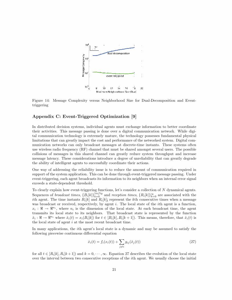
Figure 14: Message Complexity versus Neighborhood Size for Dual-Decomposition and Event-triggering
Appendix C: Event-Triggered Optimization [9]
In distributed decision systems, individual agents must exchange information to better coordinatetheir activities. This message passing is done over a digital communication network. While digi-tal communication technology is extremely mature, the technology possesses fundamental physicallimitations that can greatly impact the cost and performance of the networked system. Digital com-munication networks can only broadcast messages at discrete-time instants. These systems oftenuse wireless radio frequency (RF) channel that must be shared amongst several users. The possiblecollisions of messages in this shared channel can greatly reduce system throughput and increasemessage latency. These considerations introduce a degree of unreliability that can greatly degradethe ability of intelligent agents to successfully coordinate their actions.
One way of addressing the reliability issue is to reduce the amount of communication required insupport of the system application. This can be done through event-triggered message passing. Underevent-triggering, each agent broadcasts its information to its neighbors when an internal error signalexceeds a state-dependent threshold.
To clearly explain how event-triggering functions, let’s consider a collection of N dynamical agents.
Sequences of broadcast times, {Bi[k]}|infty
k=0and reception times, {Ri[k]}∞k=0 are associated with the
ith agent. The time instants Bi[k] and Ri[k]¡ represent the kth consecutive times when a messagewas broadcast or received, respectively, by agent i. The local state of the ith agent is a function,xi : ℜ → ℜni , where ni is the dimension of the local state. At each broadcast time, the agenttransmits its local state to its neighbors. That broadcast state is represented by the functionxi : ℜ → ℜni where xi(t) = xi(Bi[k]) for t ∈ [Bi[k], Bi[k + 1]). This means, therefore, that xi(t) isthe local state of agent i at the most recent broadcast time.
In many applications, the ith agent’s local state is a dynamic and may be assumed to satisfy thefollowing piecewise continuous differential equation
xi(t) = fi(xi(t)) +∑
j 6=i
gij(xj(t)) (27)
for all t ∈ [Ri[k], Ri[k + 1]) and k = 0, · · · ,∞. Equation 27 describes the evolution of the local stateover the interval between two consecutive receptions of the ith agent. We usually choose the initial
21

condition of this resulting state trajectory to yield a continuous trajectory when we join all of thesegments together. The function fi : ℜni → ℜni represents the ith agent’s local dynamics. Thefunction gij : ℜnj → ℜni models the communication induced dynamic coupling between the jth andith agents.
Equation 27 describes a sampled-data system in which the ith agent uses samples of its neighboringagent’s local states to help regulate its own behavior. It is possible to characterize a broadcasttime sequence {Bi[k]}∞k=0 which guarantees that this sampled-data system is semiglobal asymptot-ically stable. This characterization of the stabilizing broadcast sequence is obtained by treatingthe sampled-data system as a “discrete” approximation to a continuously-sampled system that isalready known to be input-to-state stable (ISS). The associated “continuously-sampled” system isdescribed by the system equations
xi(t) = fi(xi(t)) +∑
j 6=i
gij(xj(t)) (28)
for all t. Note that equation 28 differs from equation 27 with regard to the argument of the couplingfunction, gij . In equation 28, the ith agent has continuous access to its neighbors’ local state.
The asymptotic stability of the discretely-broadcast system is guaranteed if the continuously-broadcastsystem is input-to-state stable. In particular, this means there exists a function V : ℜn → ℜ (wheren =
∑
i ni) and class K functions (continuous and monotone increasing) αi : ℜ → ℜ and βi : ℜ → ℜsuch that
V =
N∑
i=1
∂V
∂xi
fi(xi) +∑
j 6=i
gij(xj + ej)
≤N∑
i=1
(−αi(‖xi‖) + βi(‖ei‖)) (29)
In the above equation ei represents a disturbance that enters through the gij coupling function.
Equation 29 assures that the continuous-broadcast system (equation 28) is ISS with ISS-Lyapunovfunction V . This function will become Lyapunov function for the discrete-broacast system in equa-tion 27 if it is possible to ensure that
−αi(‖xi‖) + βi(‖ei‖) ≤ 0 (30)
for all time and all i. In particular, let the disturbance ei : ℜ → ℜni be an error signal of the form
ei(t) = xi(t) − xi(t) (31)
The signal ei(t) is therefore the difference between the ith agent’s current state at time t and itsstate at the most recent broadcast time Bi[k]. At each broadcast time, Bi[k], this error is zero.So one simply needs to choose the broadcast times {Bi[k]}∞k=0 to ensure that equation 31 is alwaystrue. This can be accomplished by simply having the ith agent broadcast its local state when theinequality in equation 30 is about to be violated. In this regard, equation 30 is a threshold testautomatically ensures that V is a Lyapunov function for the sampled-data system. So that selectingbroadcast times based on equation 30 assures the asymptotic stability of the sampled-data system.
22

References
[1] K.E. Arzen. A simple event-based pid controller. In Proceedings of the 14th IFAC WorldCongress, 1999.
[2] A. R. Bergen and V. Vittal. Power Systems Analysis. Prentice-Hall, 2 edition, 2000.
[3] F.P. Kelly, A.K. Maulloo, and D.K.H. Tan. Rate control for communication networks: shadowprices, proportional fairness and stability. Journal of the Operational Research Society, 49(3):237–252, 1998.
[4] R. Lasseter. Control and design of microgrid components. Final Project Report - Power SystemsEngineering Research Center (PSERC-06-03), 2006.
[5] R.H. Lasseter, A. Akhil, C. Mrnay, J. Stephens, J. Dagle, R. Guttronson, A. Meliopoulous,R. Yinger, and J. Eto. The certs microgrid concept. White paper for transmission reliabilityprogram, office of power technolgoies, U.S. Department of Energy, 2002.
[6] M.D. Lemmon, T. Chantem, X. Hu, and M. Zyskowski. On self-triggered full information h-infinity controllers. In Hybrid Systems: computation and control, 2007.
[7] S.H. Low and D.E. Lapsley. Optimization flow control, I: basic algorithm and convergence.IEEE/ACM Transactions on Networking (TON), 7(6):861–874, 1999.
[8] P. Wan and M.D. Lemmon. Distributed network utility maximization using event-triggeredbarrier methods. submitted to the European Control Conference, 2009.
[9] X. Wang and M.D. Lemmon. Self-triggered feedback control systems with finite-gain l2 stability.to appear in the IEEE Transactions on Automatic Control, 2008.
23