Embed Size (px)
Citation preview

Atmospheric and
Environmental Research, Inc.
Final Report for
Aerosol Modeling for the Global Model Initiative
NAS5-99201
For the period May 25, 1999 to May 24, 2001
Principal InvestigatorDebra K. Weisenstein
Malcolm K.W. Ko
Atmospheric and Environmental Research, Inc.
131 Hartwell Avenue, Lexington, MA 02421-3126
March 28, 2001


Form ApprovedREPORT DOCUMENTATION PAGE OMB No. 0704-0188
Public report ng burden for this collection of information is estimated to average 1 hour per response, including the time for reviewing instructions, searching existing data sources, gathering land maintaining the data needed and completing and reviewing the collection of information. Send comments regarding this burden estimate or any other aspect of h s co lect on of _information, including suggestions'for reducing this burden, to Washington Headquarters Services, Directorate for Information Operations and Reports, 1215 Jefferson Davis Highway, Suite1204, Arlington, VA 22202-4302, and to the Office of Management and Budget, Paperwork Reduction Project (0704-0188), Washington, DC 20503.
1. AGENCY USE ONLY (Leave b/ank) 2. REPORT DATE 3. REPORT TYPE AND DATES COVERED
March 30, 2001 Final Report, May 25, 1999 to May 24, 2001
5. FUNDING NUMBERS4. TITLE AND SUBTITLE
Aerosol Modeling for the Global Model Initiative
6. AUTHORS
Debra K. Weisenstein
Malcolm K. W. Ko
7. PERFORMING ORGANIZATION NAME(S) AND ADDRESS(ES)
Atmospheric and Environmental Research, Inc.
131 Hartwell Avenue
Lexington, MA 02421
9. SPONSORING/MONITORING AGENCY NAME(S) AND ADDRESS(ES)
NASA Goddard Space Flight Center
Greenbelt, MD 20771
NAS5-99201
8. PERFORMING ORGANIZATIONREPORT NUMBER
P796
10. SPONSORING/MONITORING AGENCYREPORT NUMBER
11. SUPPLEMENTARY NOTES
12a. DISTRIBUTION/AVAILABILITY STATEMENT 12b. DISTRIBUTION CODE
13. ABSTRACT (Maximum 200 words)
The goal of this project is to develop an aerosol module to be used within the framework of the Global Modeling Initiative (GMI). The
model development work will be preformed jointly by the University of Michigan and AER, using existing aerosol models at the twoinstitutions as starting points. The GMI aerosol model will be tested, evaluated against observations, and then applied to assessment of
the effects of aircraft sulfur emissions as needed by the NASA Subsonic Assessment in 2001. The work includes the following tasks:
1. Implementation of the sulfur cycle within GM1, including sources, sinks, and aqueous conversion of sulfur. Aerosol modules will
be added as they are developed and the GMI schedule permits.
2. Addition of aerosol types other than sulfate particles, including dust, soot, organic carbon, and black carbon.
3. Development of new and more efficient parameterizations for treating sulfate aerosol nucleation, condensation, and coagulation
among different particle sizes and types.
4. Develonment of a 3-D database which can be used to evaluate results of the aerosol model.
14. SUBJECT TERMS
aerosol model
Global Model Initiative (GMI)
17. SECURITY CLASSIFICATION OFREPORT
unclassified
18. SECURITY CLASSIFICATION OFTHIS PAGE
unclassified
NSN 7540-01-280-5500
19. SECURITY CLASSIFICATION OFABSTRACT
unclassified
15. NUMBER OFPAGES
52
16. PRICECODE
20. LIMITATION OF ABSTRACT
unlimited
Computer Generated STANDARD FORM 298 (Rev 2-89)Prescribed by ANSI Std 239-18298-102


Abstract
This is the final report for a project funded by the Subsonic Assessment Program of the
Atmospheric Effects of Aviation Project to implement an aerosol prognostic capability in the
Global Modeling Initiative three-dimensional model. Though the original contract period was
reduced from 3 years to 2 years and the funding was reduced by 50%, we have accomplished
many of the original goals and are prepared to continue the work under other funding. The
work involved collaboration between Atmospheric and Environmental Research, Inc. (AER)
and the University of Michigan. The main accomplishment of the contract period was a thor-
ough intercomparison of aerosol process algorithms between the AER microphysical code and
the University of Michigan microphysical code. The AER code simulates nucleation, conden-
sation, and coagulation of sulfate aerosols using a 40 bin size distribution. This approach is
not practical for use in 3-D models because of its computational demands. The University of
Michigan code calculates the mass loading and aerosol number concentration using a 2-mode
distribution. A common set of algorithms which differ only in the method of resolving the
aerosol size distribution has now been agreed to and is described in this report. Thus we are
in a position to modify the 2-mode parameterizations to provide more realistic simulations.
The AER two-dimensional aerosol model has been updated for consistency with the common
algorithms and global calculations performed.
1 Project Overview
The goal of this project was to develop an aerosol module to be used within the framework
of the Global Modeling Initiative (GMI). The motivation came from the need to assess the
atmospheric impact of sulfur compounds and particulate matter emitted by jet engines in the
upper troposphere and lower stratosphere. The model development work was performed jointly
by the University of Michigan and AER, using existing aerosol models at the two institutions
as starting points. The GMI aerosol module was to be tested, evaluated against observations,
and then applied to assessment of the effects of aircraft sulfur emissions as needed by the NASA
Subsonic Assessment in 2001. The original scope of the work included the following tasks:
1. Implementation of the sulfur cycle within GMI, including sources, sinks, and aqueous
conversion of sulfur. Aerosol modules will be added as they are developed and the GMI
schedule permits.
2. Addition of aerosol types other than sulfate particles, including dust, soot, organic carbon,and black carbon.
3. Development of new and more efficient parameterizations for treating sulfate aerosol nu-
cleation, condensation, and coagulation among different particle sizes and types.
4. Development of a 3-D database which can be used to evaluate results of the aerosol model.
Note that the contract period was shortened from 3 to 2 years, with the total funding reduced
to half of the proposed budget. Thus the performance objectives were modified over the original
statement of work. Still, we were able to address most of the issues in the original proposal,
though item (2) above was eliminated from the project scope.
Sulfur source gas production and removal rates were delivered to GMI by Joyce Penner to
begin the process of implementing the sulfur cycle in the 3-D model (Task 1). The GMI team,
however, has been too busy to implement this yet. To accomplish Task 3, we performed inter-
comparisons between tile AER and University of Michigan aerosol aerosol models, comparing
nucleation, condensation, and coagulation codes. This resulted in updates of both model codes,
as common algorithms were agreed to. The final versions of the these algorithms are presented
in this final report. We are now confident that the model differences are due only to the method
of resolving the size distribution. Results of the model intercomparison exercises were presented
at GMI meetings in January 2000 and June 2000. A 3-D database suitable for model evaluation
(Task 4) exists at the University of Michigan and is available for model comparisons when GMI
implements our aerosol modules and generates aerosol distributions.
2 Scientific Results
2.1 Approach
The AER 2-D sulfate aerosol model is described in Weisenstein et al. [1997]. It uses 40
size bins by volume doubling from 0.39 nm to 3.2 #m. Each size bin is transported separately,
2

assuminga single constant radius. Condensation rates are calculated for eachbin size, andcoagulationdeals with the interaction of each bin sizewith all others. This model has beenusedfor the calculation of supersonicaircraft perturbations to stratosphericaerosolsurfaceareadensity (IPCC [1999], Kawa et al. [1999]) and for the study of volcanic perturbations to the
stratospheric aerosol layer ( Weisenstein et al. [1997]; Weisenstein and Yue [1999]). Nucleation
previously followed the classical formulation of Zhao and Turco [1995] but has been replaced
with the Kulmala et al. [1998] parameterization for this study. The diffusion coefficient in the
condensation algorithm has been updated according to Jacobson [1999], and the Kelvin effect
has been added.
The University of Michigan 2-mode aerosol model follows Kreidenweis and Seinfeld [1988],
Harrington and Kreidenweis [1998a], and Harrington and Kreidenweis [1998b]. The term
"mode" refers to an aerosol distribution characterized by its mean radius, number concentra-
tion, and a geometric standard deviation. The mass and number concentration of each mode
are calculated prognostically in the model. The mean radius is derived from mass and number
concentration; the standard deviation ag of the lognormal distribution is assumed. The size
distributions of the two modes may overlap, though each mode is transported separately. Mode
1 generally represents fine, submicron sized particles resulting from recent nucleation events.
Mode 2 represents coarse particles which sediment rapidly. The prognostic equations for massand number concentration include terms related to homogeneous nucleation of new sulfuric
acid/water particles, condensation of H2SO4 on preexisting sulfate aerosol, and coagulation of
sulfate aerosol particles.
It was decided at the beginning of this project that the modal approach, currently used by
the University of Michigan model, would be applied to the GMI model. The reason for this is the
efficiency of the scheme, which makes it practical for three-dimensional modeling. Only aerosol
mass and number in each mode need to be transported. The size-resolving approach used by
AER requires that the number density in each of 40 bins be transported. Adding non-sulfate
aerosol types would require an additional 40 bins for each type. The size-resolving approach does
have the advantage of more accurately dealing with aerosol sizes and the interactions among
particles. This would be particularly important in regions of nucleation and in regions suchas aircraft wakes where aerosols are added to the atmosphere. To address this issue, we have
performed model intereomparisons to analyze and improve the performance and accuracy of the
modal scheme. We also have the option of increasing the number of modes for situations where
more accuracy is required.
Because the AER and University of Michigan models differ in dimensionality and transport
parameterizations, a meaningful direct comparison was not possible. Therefore we chose to com-
pare individual aerosol processes within a box model. Realistic initial conditions were chosen,
some including an initial aerosol distribution and some initialized with only gas phase H2SO4.
Analysis of these process model intercomparisons allowed us to determine differences between
the AER and University of Michigan microphysical modeling approaches. Differences due to
nucleation, condensation, and coagulation algorithms were resolved, so that the remaining dif-
ferences are due only to the different methods of resolving the size distribution. The common
algorithms agreed to are described below.

2.2 Microphysical Algorithms
2.2.1 Nucleation
The fornmlation of homogeneousnucleation follows the parameterizationof Kulmala et al.
[1998], with the nucleation rate J (particles cm -3 s -1) given by:
J = exp(25.1289Ns,al - 4890.8Ns_gI/T - 1743.3/T
-2.24795Ns,aIRH + 7643.4xat/T - 1.9712z_JRH) (1)
with
N,u,: = ln(Na/N.,.) (2)
T - 273.15
5 = 1+ 273.15 (3)
Here Na is the ambient sulfuric acid vapor concentration, Na,c is the sulfuric acid vapor con-
centration needed to produce a nucleation rate of 1 cm-3s -1, T is temperature (K), x_z is acid
mole fraction of the embryo, and RH is fractional relative humidity. N,,c is parameterized as:
N_,_ = exp(-14.5125 + 0.1335T - 10.5462RH + 1958.4RH/T). (4)
The H2SO4 mole fraction in the critical nucleus is given by
0.0154RA
xa_ = 1.2233 RA + RH + 0.0102 In N,v - 0.0415 In Nwv + 0.0016T (5)
where RA denotes fractional relative acidity, and N,. and Nwv are sulfuric acid and water vapor
concentration (cm-a), respectively. The embryo radius r* is obtained by solving
20"?2 w
-o (6)T*
where
A#w
Vw
= -kBTln(N_v/N_,so_) (7)
= 18( + dX_ )/A, (8)
after the composition (x_t) is known. Here X_ is the mass fraction of acid in the embryo, A.
is Avogadro's number, kB is the Boltzmann constant, and p and a are the density and surface
tension of the droplet. N_:og is the equilibrium concentration of water vapor over the surface
of a solution with composition xal. The parameterizations are valid over the temperature range
from 233 K to 298 K and from 10 to 100% relative humidity. For use near the tropopause and
in the lower stratosphere, we are awaiting an updated parameterization from Kulmala.

2.2.2 Condensation
The condensation rate Gi onto Ni particles of radius ri is given by
Gi = 47r/3Ds(Ns- NSsat)riNi (9)
with
[ (1.33Kni + 0.71 4(1 - a)) ]-1 (10)
Kni = --.As (11)ri
Ds is the diffusion coefficient for HeS04 molecules in air. Ns and N sat denotes the number
density of H2S04 in the gas phase and the equilibrium H2S04 number density over the surface
of sulfate aerosol particles, respectively. N sat includes solution and curvature (Kelvin) effects
[Jacobson, 1999]. fl is the correction factor for non-continuum effects and imperfect surfaceaccommodation. Two different values for the accommodation coefficient a are currently tested:
a=l and c_=0.04. As in the equation for the Knudson number Kni denotes the mean free path
for H2SO4 molecules in air.
In the two mode model, the particle volume mean radius, r,,ol, times a correction factor is
substituted for ri above
' ri = rvotexp(-ln2cra). (12)
This corrects for the effect of the size distribution on the condensation rate of the mode. However,
the size dependence of the Knudson number Kni and of the supersaturation over a curved surface
are ignored. Potential improvements to the two mode treatment of condensation could include
a new parameterization of the correction factor or performing the condensation calculation for
multiple bins within each mode.
2.2.3 Coagulation
We only consider Brownian coagulation. For the coagulation kernel Kij between a particles
of radius ri and a particle of radius rj, we apply the interpolation formula of Fuchs [1964]:
Kij = 47r(Di+ Dj)(ri+ri)
( r_+rj 4(Di+Dj) )-1a2'_a/2 + (13)r i Ac rj -4- (g2 _[_ YJ; (C 2 "_ C2) 1/2 (r i At rj)
0.87 ]kBT 1 + Kna,i(1.249+0.42 exp(-K-_,/)) j (14)with Di - 6 zr r/, ri
Kna,i = --Aa (15)ri
gi = 2 (ri -4- li) 3 -- (r/2 nt- /2)3/2 _ 2ri (16)3 rili

4 Dili = --
7r c i
C i = ....
k Trmi ]
1/2
(17)
(18)
ku and T denote the Boltzmann constant and the temperature. Aa is the mean free path of air
molecules, r/a the dynamic viscosity, and mi the mass of a particle of radius ri.
In the 40 bin model, coagulation between two particles in the same bin results in one particle
in the next larger bin. Coagulation between one particle and another particle from a smaller
bin results in a fraction of the combined particle mass in the original larger bin and the next
larger bin. In the two mode model, coagulation between two particles in the same mode results
in a reduction in number density in that mode, but no mass change in that mode. Coagulation
between particles in different modes results in mass transfer to the larger mode. A scheme to
shift mass between modes as coagulation occurs has been implemented but needs further testingand refinement.
2.3 Box Model Intercomparison
The most important milestone in the first year of our project involved a model intercompar-
ison of the two mode model and the 40 bin model. We first performed the comparisons using
four sets of initial conditions, designated Box 1 through Box, 4. Relative humidities varied from
0.66% to 95%, temperatures from 208 K to 263 K, and pressure levels were either 200 or 500
mb. Each model used these initial conditions without transport and reported initial tendencies
and time evolution of the aerosol distribution for a 24 hour period. Tables 1-4 show the initial
conditions and initial rates for nucleation, condensation, and coagulation (Boxes 1 and 2 have
no initial condensation or coagulation because there was no initial aerosol). This exercise re-
sulted in many algorithm updates for both models as standard formulations were agreed to and
differences resolved. We are now confident that the differences between model results derive
solely from the different ways of treating the size distribution.
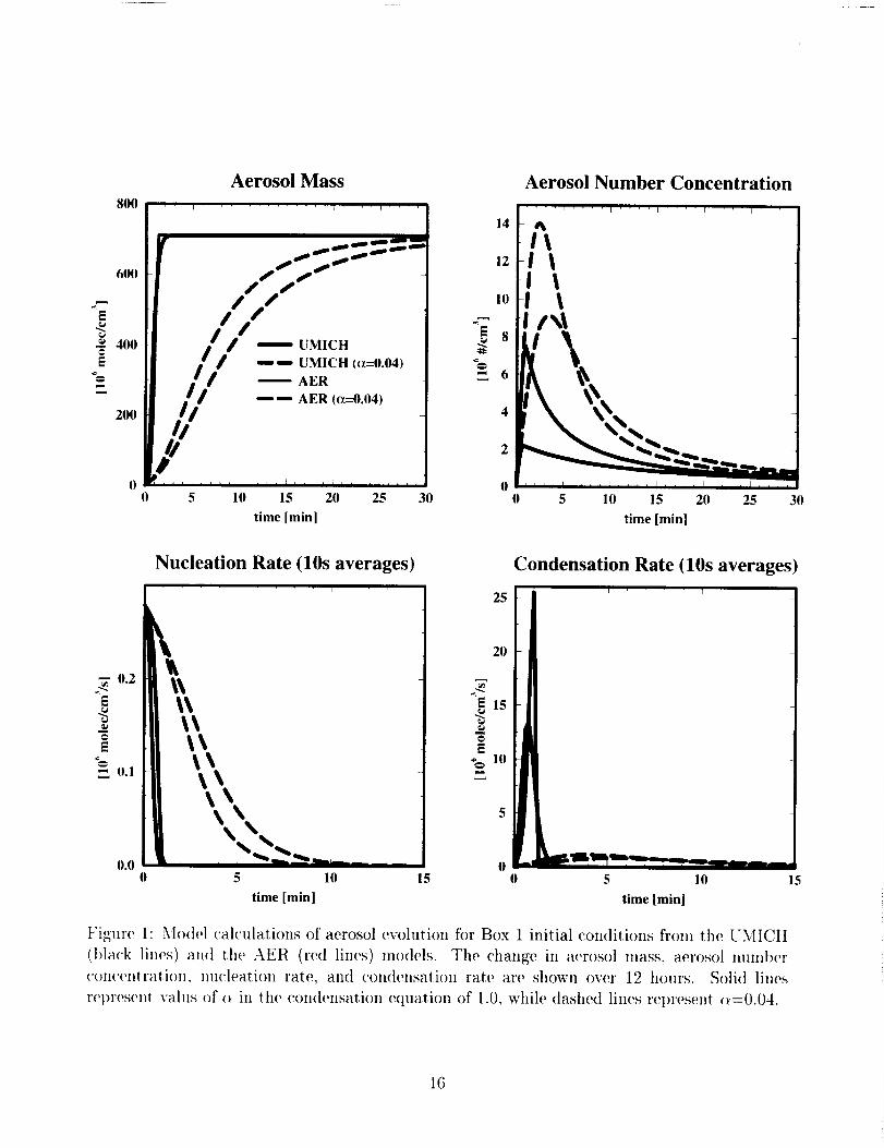
The Figures 1-4 represent the time evolution of aerosol mass, number, nucleation rate, and
condensation rate over 24 hours for each of the four initial conditions. Results from the two
mode model (labeled UMICH) and the 40 bin model (labeled AER) are shown with values
of a in the condensation equation of 1.0 and 0.04. The value of a used in the condensation
equation has generally been 1.0, which implies that all collisions between gas phase H2SO4 and
aerosol particles result in particle growth. With a value of c_ of 0.04, the condensation rate is
dramatically reduced and the time required for gas-to-particle transfer is increased from 1 hour
to 30 hours in Box 1 and from 1 hour to 12 hours in Box 4. Differences in the treatment of
condensation (because of the different ways of representing the size distribution) are apparent
and result in different number concentrations after integration.
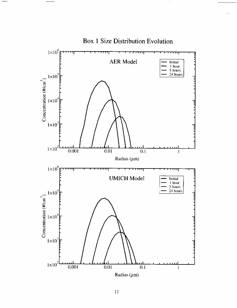
Figures 5-8 show the initial aerosol size distributions as a function of radius and those calcu-
lated by each model during and at the end of the model integration for the case where c_=l.0.
Box 1 results show that the two mode model accurately reproduces the size distribution in the
situation where all aerosols are nucleated within the first minute and condensation ceases after
2 minutes due to depletion of gas phase H2SQ. A single-mode log-normal distribution results
after 1 hour due to coagulation, though the width of the distribution is somewhat narrower in
6

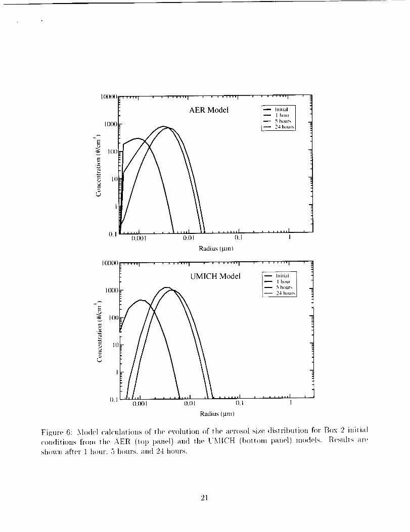
the 40 bin model than the two mode model. In Box 2, nucleation continues for 5 hours and
the final aerosol mass is reached after 10 hours. In this case, the 40 bin model shows a skewed
distribution after 1 and 5 hours due to continued particle generation in the smallest size bin,
while the two mode model shows the same peak number density, but a symmetrical distribution.
Box 3 was initialized with a three-mode size distribution, and subsequent changes in total
aerosol mass were minor. Both models show no change in the size distribution over 24 hours,
but the two mode model fits the initial distribution into a single mode, so the initial shape is
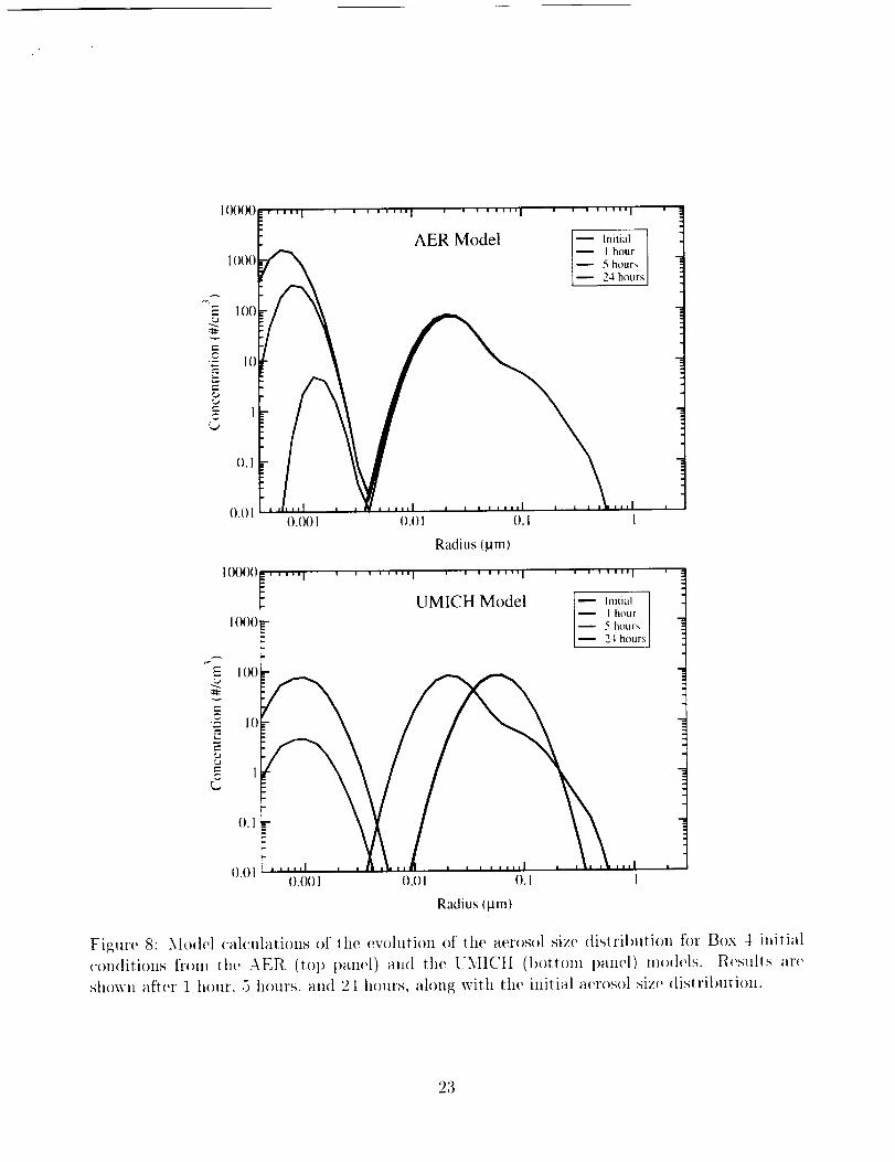
not preserved. Box 4 had an initial aerosol distribution along with nucleation and condensation
for the first hour, though the total aerosol mass increased by only 1% in the 24 hour period.
The two mode model fit the initial aerosols into mode 2 and the newly nucleated aerosols into
mode 1. The particle number densities in mode 1 after 1 and 5 hours are much less than in the
40 bin model, and by 24 hours all mode 1 particles have been shifted into mode 2.
We repeated the Box 4 calculations using a single lognormal distribution (rather than a
superposition of three lognormals) as the initial condition. Figure 9 shows results of the Box
4 calculation of aerosol mass, number concentration, nucleation rate, and condensation rate
with the revised initialization. The AER results shown in red used the original initial aerosol
distribution, which assumed 90% of the initial particles in a lognormal distribution with mode
radius of 0.021 #m, 10% of the initial particles in a lognormal distribution with mode radius
of 0.069 #m, and 0.04% of the initial particles in a lognormal distribution with mode radius
of 0.351 #m. The green line represents a calculation performed with a single lognormal initial
distribution with mode radius of 0.043 #m. The UMICH model, since it fits the initial aerosol
distribution into the larger of its two modes, can only represent the initial distribution as a
single lognormal. Aerosol number concentration differs most between the models. AER model
results using a single lognormal initial distribution (green lines) are considerably closer to the
UMICH values than the standard AER results (shown in red). We find better agreement since
the 2-mode model now accurately represents the initial distribution. However, compared to the
AER model, the 2-mode model often overestimate condensation and underestimates coagulation
rates. Some of this difference is likely due to the different timestepping schemes employed by
the two models: an explicit scheme for AER and an implicit scheme for UMICH.
An additional intercomparison exercise involved using a range of actual zonal mean and
extreme conditions for January and performing 24 hour aerosol integrations. The calculations
are for four altitudes (850, 500, 200, and 50 mb) and a range of latitudes. Figure 10 shows a
scatter diagram of AER results vs. UMICH (labeled Bimodam) results as originally calculated
in November 1999. Total particle number, nucleation over 24 hours, and condensation over 24
hours are shown. The plots show that agreement between the models was reached only for a
limited subset of conditions. Figure 11 shows current results after the models were updated to
similar microphysics. Agreement is much improved and falls within reasonable limits for all but
a few conditions. These results were presented at the International Conference on Nucleation
and Atmospheric Aerosols by Michael Herzog.
2.4 Enhancements to the AER 2-D Sulfate Aerosol Model
Updates to the AER aerosol model have included implementation of new microphysical
algorithms to match those agreed to for GMI and improvements to the 2-D transport and
chemistry. The AER 2-D sulfate aerosol model and the AER 2-D chemistry transport model have
7

beencombinedinto one model. Previously thesewere separatemodels,with the sulfate modelusing input OH and Oafrom the chemistrymodel and the chemistry modelusing input surfacearea density from the sulfatemodel. With the modelscombined,perturbation calculations canbe done with a singlecalculation rather than a seriesof two or moredifferent calculations. Forexample,a Mt. Pinatubo calculation cancalculatechangesin sulfatesurfaceareadensity whichwill impact ozonein the samecalculation. While this currently haslittle effecton model results,it will allow for greater interactivity of sulfateand other trace gasesin the future. For example,wecould allow HNOa to condenseonto sulfateaerosolsand generatePSCsof STScomposition.This developmentwork on the AER 2-D sulfateaerosolmodel was fundedlargely through ourSAGE II contract (NAS1-99096)but is of benefit to this contract also.
Convectionhas beenadded to the AER 2-D model, using codeand data filesobtained fromVictor Dvortsov [Dvortsov et al., 1998] and based on CCM3 convective fluxes. We found the
convection to work well with the transport circulation of the GSFC 2-D model, as this transport
is based on observational data. With the AER transport, which includes an enhanced Kzz
term to partially account for convection, inclusion of the convective parameterization results in
too much tracer transport between the surface and the upper troposphere. Figures 12 and 13
show model-calculated aerosol extinction at 1.02 ttm and aerosol surface area density without
(panel a) and with (panel b) convection. The calculated extinction with convection agrees well
with SAGE observations for nonvolcanic periods. Aerosol surface area density is considerably
enhanced by convection in the lower stratosphere, and may be somewhat too large compared toobservations.
The time stepping scheme in our 2-D aerosol model uses time splitting and performs nu-
cleation before condensation. In cases with both large nucleation and condensation rates, the
gas phase H2SO4 may be used up by nucleation and none left for condensation. Observational
results indicate that under conditions with ample available surface area for condensation, the
effects of nucleation are limited [Kulmala et al., 2000]. We have explored this issue in the global
2-D model by modifying the time stepping scheme. Figure 14a shows the annual average aerosol
surface area density calculated by the model in its normal mode, where the nucleation step is
performed before the condensation step. Figure 14b shows results with the condensation step
performed first. Performing nucleation first results in 20-30% greater aerosol surface area density
in the upper tropical troposphere. To help assess the accuracy of these schemes, we have subdi-
vided the 1 hour time step into 40 substeps doing condensation and nucleation in sequence. The
calculated surface area density with this scheme is shown in Figure 14c and falls between those
shown in Figures 14a and 14b. This should represent a fairly accurate time-stepping scheme,
though the computational time required is prohibitive. A new scheme has been devised which
calculates the rate of change of gas phase H2SO4 due to nucleation and condensation (before
modifying the aerosol number densities) and subdivides the time step if nucleation and/or con-
densation will deplete all H2SO4 within a single time step. Results of this scheme are shown
in Figure 14d. The computer time required for this scheme is quite modest because only grid
points with large aerosol changes will perform a maximum of 50 substeps.
Tile condensation and nucleation routines of the model have also been updated. Updates to
the condensation rate include correction of the effective mean free path and diffusion coefficient
according to Jacobson [1999], introduction of the Kelvin effect, and use of saturation vapor
pressures from Ayers et al. [1980] and sulfuric acid activity coefficients from Taleb et al. [1996]
as parameterized in Kulmala et al. [1998]. Tile impact of these changes on calculated annual
8

averagesurfaceareadensity for nonvolcanicconditions is shownin Figure 15,where15ausestheold condensationroutine and 15bthe newroutine. The most obviousimpact is due to the Kelvineffectand results in a smaller surfacearea density at high latitudes and high altitudes. Useofupdatedvapor pressuresin the condensationschemehasvery little effecton calculated surfaceareadensity. It doeshavean impact, however,on nucleationrates. Figure 15cshowssurfaceareadensity calculated with the new vapor pressuresused in the Zhao and Turco [1995] nucleation
scheme. Surface area density increases by 30-40% in the tropical upper troposphere with use of
the updated vapor pressures. Figure 15d shows a calculation using the Kulmala et al. [1998]
nucleation parameterization for grid points where the relative humidity is greater than 10%
and the classical nucleation approach for all other cases. The Kulmala et al. parameterization
includes the effects of hydration, which our classical approach does not. The nucleation rate
in the troposphere is smaller with the Kulmala et al. parameterization, and thus surface area
densities are smaller.
2.5 Future Directions
Implementation of a prognostic aerosol scheme for GMI should continue to be a high priority.
The GMI model in the future will have the capability to adequately handle problems involv-
ing both stratospheric and tropospheric chemistry and transport. Many problems involving
atmospheric sulfate and aerosols (volcanic effects, aircraft impacts) will require both a realistic
troposphere and a realistic stratosphere. If GMI funding continues, we are prepared to imple-
ment the 2-mode aerosol module within GMI. The algorithms described here are the appropriate
first step, but can be improved by increasing the number of modes (after model analysis to de-
termine the optimum number), adding other aerosol types (dust, soot, black carbon, organic
carbon), and developing parameterizations for the interaction of these aerosol types.
3 Deliverables
Source emission rates and chemical rate constants required to calculated gas phase sulfur
chemistry were delivered to GMI by Joyce Penner. An aerosol database which will be used to
compare three-dimensional calculated aerosol distributions with observations is available at the
University of Michigan. Aerosol microphysical parameterizations are available as fortran code
and can be delivered to the GMI team at Lawrence Livermore National Laboratory on short
notice.
The following presentations were related to this contract:
1. given by Joyce Penner at the January 2000 GMI Meeting in Washington, DC [Penner et
al., 2000];
2. given by Debra Weisenstein at the June 2000 GMI and AEAP Meeting, Snowmass, CO
[ Weisenstein et al., 2000];
3. given by Michael Herzog at the International Conference on Nucleation and Atmospheric
Aerosols, Rolla, MO [Herzog et al., 2000a; 2000b].

References
Ayers, G. P., R. W. Gillett, and J. L. Gras, On the vapor pressure of sulphuric acid, Geophys.
Res. Lett., 7, 433-436, 1980.
Dvortsov, V. L., M. A. Geller, V. A. Yudin, and S. P. Smyshlyaev, Parameterization of the
convective transport in a two-dimensional chemistry-transport model and its validation with
radon 222 and other tracer simulations, J. Geophys. Res., 103, 22,047-22,062, 1998.
Fuchs, N. A., Mechanics of aerosols, Pergamon Press, New York, 1964.
Harrington, D. Y., and S. M. Kreidenweis, Simulations of sulfate aerosol dynamics - I. Model
description, Atmos. Env., 32, 1691-1700, 1998a.
Harrington, D. Y., and S. M. Kreidenweis, Simulations of sulfate aerosol dynamics - II. Model
intercomparisons, Atmos. Env., 32, 1701-1709, 1998b.
Herzog, M., J. E. Penner, J. J. Walton, S. M. Kreidenweis, D. Y. Harrington, D. K. Weisenstein,
Modeling of Global Sulfate Aerosol Number Concentrations, Talk presented at the 15th
International Conference on Nucleation and Atmospheric Aerosols, University of Missouri,
Rolla, MO, August 6-11, 2000a.
Herzog, M., J. E. Penner, J. J. Walton, S. M. Kreidenweis, D. Y. Harrington, D. K. Weisen-
stein, Modeling of Global Sulfate Aerosol Number Concentrations, in B. N. Hale and M.
Kulmala, eds, Nucleation and Atmopheric Aerosols 2000: 15th International Conference,
AIP Conference Proceedings, Vol. 53_, pp. 677-679, 2000b.
Intergovernmental Panel on Climate Change (IPCC), Aviation and the Global Atmosphere,Cambridge University Press, 1999.
Jacobson, M. Z., Fundamentals of Atmospheric Modeling, Cambridge University Press, Cam-
bridge, U. K., 1999.
Kawa, S. R., et al., Assessment of the Effects of High-Speed Aircraft in the Stratosphere: 1998,
NASA//TP-1999-20923Z 1999.
Kreidenweis, S. M. and J. H. Seinfeld, Nucleation of sulfuric acid-water and methane sulfonic
acid-water solution particles: Implications for the atmospheric chemistry of organosulfur
species, Atmos. Env., 22, 283-296, 1988.
Kulmala, M., A. Laaksonen, and L. Pirjola, Parameterizations for sulfuric acid/water nucleation
rates, J. Geophys. Res., 103, 8301-8307, 1998.
Kulmala, M., L. Pirjola, and J. M. M/ikel_i, Stable sulphate clusters as a source of new atmo-
spheric particles, Nature, _0_, 66-69, 2000.
Penner, J. E., M. Herzog, D. K. Weisenstein, M. K. W. Ko, Progress on an aerosol module
for the Global Modeling Initiative, GMI Science Team Meeting, Washington, DC, Jan. 4-6,2000.
Taleb, D.-E., J.-L. Ponche, and P. Mirabel, Vapor pressures in the ternary system water-nitric
acid-sulfuric acid at low temperature: A reexamination, J. Geophys. Res., 101, 25,967-
25,977, 1996.
Weisenstein, D. K., G. K. Yue, M. K. W. Ko, N.-D. Sze, J. M. Rodriguez, and C. J. Scott, A
two-dimensional model of sulfur species and aerosols, J. Geophys. Res., 102, 13,019-13035,1997.
Weisenstein, D. K., G. K. Yue, A model study of the evolution of aerosol mass and surface
area in the post-Pinatubo period, presented at the AGU Fall Meeting, San Francisco, CA,
December 13-17, 1999.
10

Weisenstein,D. K., M. K. W. Ko, J. E. Penner, and M. Herzog, An aerosolmodule for theGlobal Modeling Initiative, presentedat the Atmospheric Effects of Aviation Conference,Snowmass,CO, June 5-9,2000.
Zhao, J., and R. P. Turco, Nucleation simulations in the wakeof a jet aircraft in stratosphericflight, J. Aerosol Sci., 26, 779-795, 1995.
11

Table 1: Initial Conditions and Initial Rates for Box 1
Quantity Units UMich Value AER Value
Initial Conditions
Pressure [mb] 500
Temperature [K] 262.96
Rel. humidity [%] 86.57
Rel. acidity [%] 13.10
H20 gas [molec/cm 3] 6.719 x 10¹⁶
H2SO4 gas [molec/cm 3] 7.097 x 10 °s
Aerosol mass [molec/cm 3] 0.0
H2SO4 mass fraction 0.2078
Aerosol density [g/cm 3] 1.1632
Nucleation
Nucleation rate [molec/cm3/s] 8.705x 10 °4
Density of nucleus [g/cm 3] 1.562
Radius of nucleus [#m] 5.006 x 10 -°4
Size of nucleus [molec/particle] 3.199
500
262.96
86.57
13.11
6.723x 10¹⁶
7.100 x 10 °s
0.0
0.2078
1.1632
8.722 x 10 o4
1.562
5.001 × 10 -04
3.192
12

Table 2: Initial Conditions and Initial Rates for Box 2
Quantity Units UMich Value AER Value
Pressure
Temperature
Rel. humidity
Rel. acidity
H20 gas
H2SO4 gasAerosol mass
H2SO4 mass fraction
Aerosol density
Nucleation rate
Density of nucleus
Radius of nucleus
Size of nucleus
Initial Conditions
[rob] 200 200
[K] 233.93 233.93
[%] 0.66 0.66
[%] 27.89 27.89
[molec/cm 3] 4.197x 10¹³ 4.299x 2013
[molec/cm 3] 2.407 × 1007 2.408 × 20 07
[molec/cm a] 0.0 0.0
0.7486 0.7486
[g/cm 3] 1.6992 1.727
Nucleation
[molec/cm3/s] 0.590 0.591
[g/cm 3] 1.805 1.806
[pin] 4.272 X 10 -04 4.267 x 10 .04
[molec/particle] 3.199 2.946
13

Table 3: Initial Conditions and Initial Rates for Box 3
Quantity Units UMich Value AER Value
Pressure
Temperature
Rel. humidity
Rel. acidity
H20 gas
H2SO4 gas
Aerosol mass
Aerosol number
Aerosol avg. radius
H2SO4 mass fraction
Aerosol density
Nucleation rate
Density of nucleus
Radius of nucleus
Size of nucleus
H2SO4 saturation
Mean free path
H2SO4 gas diff. coeff.
Condensation rate
Particle velocity
Coag. Kernel
Number Change
Initial Conditions
[mb] 500
[K] 208.12
[%] 6.366
[%] 100
[molec / cm 3] 2.206 x 10¹³
[molec/cm 3] 2.603× 10 o5
[molec/cm 3] 3.850× 10 °7
[cm -3] 8.503
[#m] 5.670x 10 .02
0.6168
[g/cm a] 1.541
Nucleation
[molec/cm3/s] 6.102x10 -°s
[g/cm 3] 1.7905
[#m] 3.064 x 10 -04
[molec/particle] 1.032
Condensation
[mo lec / cm 3] 3.056 x 10 -03
[cm] 3.328 x 10 -°5
[cm2/s] 9.119x10 -°2
[molec / cm3/s] 7.1213
Coagulation
[cm/s] 7.823
[cm 3] 1.137 × 10 .9
[cm -3 s -1] -8.224x 10 -s
500
208.12
6.366
i00
2.206x 10¹³
2.603x 1005
3.851x 10 07
8.259
5.701× 10 -02
0.6168
1.587
6.102× I0-°s
1.766
3.061×10 -04
1.030
3.051×I0 -o3
3.327× 10-06
9.124x 10 -02
3.659
7.707
1.301x10 -09
-9.121x10 -0s
14

Table 4: Initial Conditions and Initial Rates for Box 4
Quantity Units UMich Value AER Value
Pressure
Temperature
Rel. humidity
Rel. acidity
H20 gas
H2SO4 gas
Aerosol mass
Aerosol number
Aerosol avg. radius
H2304 mass fraction
Aerosol density
Nucleation rate
Density of nucleus
Radius of imcleus
Size of nucleus
H2SO4 saturation
Mean free path
H2SO4 gas diff. coeff.
Condensation rate
Particle velocity
Coag. Kernel
Number Change
Initial Conditions
[rob] 200 200
[K] 218.05 218.05
[%] 95.43 95.43
[%] 100 100
[molec/cm a] 1.110xl015 1.110×10¹⁵
[molec/cm 3] 2.293 x 10 °_ 2.293 x 10 (/_
[molec/cm a] 2.484 x 10 °s 2.485 x 10 °s
[cm-3] 411.08 402.99
[#m] 5.700 x 10 -°_ 5.701 x 10 -()2
0.1163 0.1163
[g/cm a] 1.091 1.113
Nucleation
[molec/cm3/s] 3.688 3.689
[g/cm a] 1.650 1.636
[#m] 3.609× 10 -°4 3.606× 10 -4
[molec/particle] 1.346 1.343
Condensation
[molec/cm 3] 1.458× 10 -ll 1.457× 10 -ll
[cm] 8.718 x 10 -06 8.715 x 10 -()6
[cm2/s] 0.244 0.245
[molec/cm3/s] 4432 2431
Coagulation
[cm/s] 9.517 9.419
[cm a] 2.122 x 10 -0 2.408 x 10 -o9
[cm -a s -1] -3.587x 10 -4 -3.678x 10 -04
15
Aerosol Mass Aerosol Number Concentration
800 .... I .... r .... r r I r _ P I [ ....
4,.i\/ t
400 a f I UMICH 8
=c ia / i "" '_' UMICH (_=0.04) Itl / / _ AER t 6
= II /J ---- AER (o[=0.04) /
20"ilg I 4
0 0
0 5 10 15 20 25 30 0 5 10 ! 5 20 25 30
time [mini time [mini
Nucleation Rate (10s averages) Condensation Rate (10s averages)
25
20
0.2 .]"E
i ) ,o
00 5 10 15 0 5 10 15
time [min] time [rain]
Figure 1: Model calculations of aerosol evolution for Box 1 initial conditions fl'om the UMICH
(lflack lines) and the AER (red lines) models. The change in aerosol mass. aerosol number
concentration, nucleation rate, and condensation rate are shown over 12 hours. Solid lines
represent vahls of _ in the condensation equation of 1.0, while dashed lines repI'eSellt (_=0.04.
16

10
C
5
Aerosol Mass
UMICH
UMICH (_--0.04)AER
AER (c_--0.04)
3t)000
,., 20000E
0
Aerosol Number Concentration
.... I .... L .... [ ' ' • I '
0 5 10 15 20 0 5 10 15 20
time [h] time [h]
Nucleation Rate (10s averages) Condensation Rate (10s averages)2.0 1000
i mm_ !.0
"_ i 41)0
0.5200
0.0 00 5 10 15 20 0 5 10 15 20
time [hi time [h]
Figure 2: Model (:alculati(ms of aerosol evolution fi)r Box 2 initial (-(mditions from the U._IICH
(black lines) and the AER (red lines) nm(Ms. The ('hange in aerosol mass, aerosol numbm'
concentration, nuch'ation rate. an(l condensation rate are shown over 2=1 hours. Solid lines
tel)resent valus of :_ in the ctmdensati<m equation t)f 1,0. while dashed lines represent e_=().()4.
17

38.7
2_ 38.6
E%
38.5
38.4
Aerosol Mass
8.6
8.5
8.3
8.20 5 10 15 20 0
time [hi
Aerosol Number Concentration
.... [ , r i .... _ .... r r r
I I I [ I I I h [ I I I I [ I I h I I I I I
5 10 15 20
time [hi
E
8e-08
6e -08
4e-08
2e-08
0e+00
Nucleation Rate (10s averages)8
E34
E
o 5 l0 15 2O o 5
time [h]
Condensation Rate (10s averages)
10 15 20
time [hi
Figure 3: Model calculations of aerosol evolution for Box 3 initial conditions ff()m the UMICH
(black lines) and the AER (red lines) models. The change in aerosol mass, aerosol tmmt)er('()ncentratioll. nu(:leation rate, and condensation rate are shown over 24 hours. Solid lines
tel)resent valus of (_' in the (,ondensation equation of 1.0, while (lashed lines ret)resent _=0.04.
18

251
250E
E%"_ 249
248
Aerosol Mass
0 3 6 9 12
time [hi
Aerosol Number Concentration
40000
300O0
10t_)
00 3 6 9 12
time [hi
Nucleation Rate (10s averages) Condensation Rate (10s averages)5 5000
4 4(NX)
1 1000
0 00 3 6 0 3
time [h] time [h]
Figure 4: Model (:ah:ulations of aerosol evohltion fl)r Box 4 initial conditions fr()m the U_IICH
l])]ack li)w.s) _)_1 tJw AEt_ (red ]ine,,Q models. The change i_ aero.so] mas,s, aero.sr)l )))m_l)('r
('()nt'entrati()n, ml(:h,ati()n rate, a Il(t (:on(h,nsation rate at(' shown ov(,r 12 hours. Solid lines
rol)ro._(')It vahl,_ (_f () iz_ tho (:ondensatio)i (,quation ()f 1.0, whih' da._ho(i ]i))(,s r('l)resent ()=0.04.
19

Ix 10'_
lxlO:'
E
e-
._ 1×10 4
¢)
e--
1×10 3
lxlO-
lxlO ('
1xlO 5
E:J
e--
.z._ Ixl() 4
e,.,
C
Ix 10 3
:1 iiii I , , ,,1,, I i i , , ,,_,| , . . . i,,, I
AER Model __ Initial
I hour
5 hours24 hours
. .,.,I , ,,,.I , , , , J,J,l
O.(X) 1 0.01 O, I 1
:1 Illl[
=
IIIll
().(X) I
Radius (gm)
........ I ........ I ........ I
UMICH Model [-- Initial t
l- I hour ]5 hours [
24 hours]
lxlO z ........ I10.01
Radius (_tm)
Figure 5: Model ('alculati()ns of t,h(, evolution of the aerosol size distribution for Box 1 initial
(,on(litions from t h(, AE1R (top panel) and the UMICH (bottom panel) models. Results areshown after 1 horn'. 5 hours, and 24 hours.
2O
1IX)()()
E
IO()()
I00
iO,
1
0.10.001 0.01 O.] 1
Radius (lam)
I0000 : ..... t ........ I ........ i '
I(XX)
"_" 1O0
I0
5
1
O.l
UMICH Model
O.(X)1 0.01
| | i IIll i
Initial
I hour [
5 hour,,
24 hours
I i _,,Jl j , , i ,,,,I
O.I I
Radius (Urn)
Figure 6: Model calculations of tile evolution of the aerosol size distribution fi)r Box 2 initial
conditions from the AER (top panel) and the UMICH (bottom panel) models. Results are
sh_>xvn after 1 hour, 5 hours, and 24 hours.
21

100i,
10 L
=_
c-
O
¢-O. 1
¢-
0.01
0.001
1(X)
10
E
I
O. 1
0.0 I
0.001
i |1_[
i i lIB I
' ' ' ''"1 ' ' ' ' ''"1
AER Model
| i w i i iii] i ._
JInitial ]
I hour [
5 hours24 hours
| | |
0.01 O.I
Radius (tam)
ii1|[
!
....... I ........ I
UMICH Model
i i i , i |it[
Initial1 hour
5 hours24 hours
0.00 ! 0.01 O. I I
Radius (tam)
Figure 7: Model cal(:ulations of the evolution of the aerosol size distribution for Box 3 initial
(:()n(litions fi'om the AER (top panel) an(l the UMICH (bottonl t)anel) mo(l(,ls. Results ar(,
shown after 1 hour, 5 hours, and 24 hours, along with the initial aerosol size (listril)uti()n.
22
jl
AER Model
0.01
UMICH Model
23

251
250
E
E%-_ 249
2480 3
Box 4 no gas sourceAerosol Mass
UMICH
_--, UMICH (or=0.04)
AER
---- AER (t_=0.04)
AER (one mode)
6 9
time [h]
40000
30000
"_ 20000
10000
012
Aerosol Number Concentration
0 3 6 9 12
time [hi
Nucleation Rate (10s averages)
5
4
2
1
00 3 6
time [hi
5000
4000
._ 3o00
=_ 2000
1000
Condensation Rate (10s averages)
0 3 6
time [hi
Figure 9: Model calculations of aerosol evolution for Box 4 initial conditions from the UMICH
(black lines) and the AER (red lines) models. The change in aerosol mass. aerosol tmmber
concentration, mu,leation rate, and condensation rate are shown over 6 or 12 hours. Solid lines
represent values of, in the condensation equation of 1.0, while dashed lines represent ,.=0.04.
Ih,sults from the AER model using only one lognormal mode for the initial condition are shown
in green.
24

Box Model Comparison: ]first try
Total Particle Number
$
ee
.<
106
lO s
104
10 -_
102
10 I
10"
10"11
after 24h, January, extreme values
_///
O 50mb <>_
O I"1200mb J: @1_ <>500mb /_ll_v"
A850mb .///
/
' '_ l'_ "i'o_ 10' "i'_" lo' io"Bimodam [#/cm _]
10 u
!0 _
,_ 10 7
ce
10 5
I IIs
10 _
IO'10 a_"L'iOf_i'O' "'_10 "_v "t'O 7
Bimodam [molec/cm _ day ]
Nucleation
over 24h, January. extreme values
0 50m ill[_idl[
[] 200m b
:= :f/j//'
/ i/
I0" 10 N
$
Condensation
lO u
10 7
i0 -_
10 _
!0 _
I0 -_iO l
over 24h, January. extreme values
.................. %!ii
'0 50m'b i
1-1200mb .It_W',_
0500mb ,.fi_._
A850mb ,_/"<_ '_
I0""_ "'5o'_ Io_ l."t
Bimodam [molec/cm day]
Figure 10: Scatter diagrani of total particle nunlt)er, nucleation rate, and condensation rate after
it 324 }lOllr calculation with the AER and UXIICH models. Results represent Iiio ill'st coniparis<in
of flit' iIlodol,_ in N()VOlll})(_l' 1999.
25

I0 tl
lO _
._ 10 7
E
l0 s
E
_e 10 _
Box Model Comparison Today [after corrections and improvements I
Total Particle Number
l0 s
104
i0 -_
102
c_.<
10'
10"
10 "i
I0"
after 24h, January, extreme values
O 50mb <> /_/
n200mb X/_ /
Y. °0:by
//f °10° 10' 102 10"_ 104 10"_
UMICH [#/cm _]
10'
10 -I10'
Nucleation
over 24h, January, extreme values
...................... /_^///
O 50mb A Z///_/_
[] 200m b ////_/
<> 500m b _.t//A850mb •
10' 10 _ 10 _ 107 10" 10"
UMICH [molec/cm 3 day]
lO II
10 _
-.N 10 7
_ 10 5
l0 s
lO tI0'
Condensation
over 24h, January, extreme values
- :i ........2C] 200mb
O500mb
A 850mb
to, to-_ ,;"'- ,;"- ,o,,UMICH [molec/cm _ day]
Figure 11: Scatter diagram of total particle number, uucleation rate, and condensation rate after
a 24 hour calculation with the AER and UMICH models. Results represent a comparison of the
current models after corrections and improvement to synchronize the microphysical treatment.
26

(a)
3O
4o 1(b) -o1_ °1_-°1-
a
_" --6.o--__ <..z:z__,_c.o •20 -:, -10. _U.o _-----8.0-"el
90as 60os 30°S EQ 30 °N 60°N )O°NLaLitude
Figure 12: Calculated 1.02 /,m aerosol extinction (10 -s km-1) for April under nonvolcanic
conditions. The GSFC transport is used within the AER 2-D sulfate model, and panel (b) also
includes the convective parameterization of Dvortsov et al. [1998].
27

35
(a)SO
_" 25
,__20
G9
15.Wll_
,.+..a
•_ 10
__0 -_ _0.2-
____o.__° __o.4_•0.6____0 "6-
--°8_-_.o_o_-_.o_
--i.__ (__ ----
\@
90°S 60°S S0°S EQ SOON 60°N 90°NLatitude
(b)35
3O
"_" 25
20(D
15
<_ 10
5
90°S
i ' ' I ' ' I ' ' I ' ' I ' ' I ' ' l
0. _- __---Z-7-----_.
• o.6---_2__I
• 3.0-
) S] )1 & '_"\\ 'e_bo c6 _
60°S 30°S EQ 30°N 60°N 90°NLaf.if.ude
Figure 13: Calculated annual average aerosol surface area density (#m 2 cm-3) under nonvol-
canic conditions. The GSFC transport is used within the AER 2-D sulfate model, and panel
(b) also includes the convective parameterization of Dvortsov et el. [1998].
28

40_'' ''' I '_---1-_' , ,--r--
oLot-_" o__t_-- .4 0.4-
_0.6 _06-
1.5--------_.0_
_--77/_c___7 ---
20
i0
90os 60os 30°S EQ 30 °N 60°N 9°°NLatitude
40 _ I ' _ 1 ' ' I ' ' I ' ' I ' '
.---. 30 --0.2" _0.4______________0.4.--------0.4 _
_0 6 .6-
20 -_i o_---/----_-_-i.°--
<_o.__.o f't _7 -_I
i ¢_1"1 I
90°S 60os 30°S EQ 30 °N 60°N 90°NLatitude
40 , i i , , i i i i , , i i , i , ,
.._/
30 --0.2__-_. _ ,,_0. 4---------.------_0.4-
_o 6_°6---
,._,.o--/<....._o/...----,,j___,
IlL, I ,90os 60os 30°S EQ 30°N 60°N 90°N
Latitude
40
(d)3O
_) 2O
I0
_ _0. i-O. 1_0.2__
--0.2________0.4_/---0" g----------_ 0.4 -
_0.6 0.6-
.__'*,t°_./,..___-_..______.___-
_\',,, /% <_.<_(_\\ I J "-'-" "r....e CO
o o o ,_-
90os 60oS 30°S EQ 30 °N 60°N 90°NLatitude
Figure 14: Calculated annual average aerosol surface area (#m2/cm 3) from the AER 2-D model
using GSFC transport parameters and convection. Panel (a) is with nucleation performed before
condensation, panel (b) is with condensation performed first, panel (e) is with condensation and
then nucleation performed consecutively in a substep loop 40 times per hourly advective step,
and panel (d) is with the new time stepping scheme.
29

40 _ _ I _ ' I _ _ I ' i I i _ 1 _
(a) -o.1_ _o.i.0. t _ 0.2-
.---, 30 --0.2_--------0,4-----_0" "/--------_0 •4 -
_06 06-
Q) 20-
< lo- -__---_--_:°x_ -_
90°S 60°S 30°S Eq 30°N 60°N 90°NLatitude
40 ' ' I ' ' I _ ' I ' ' I J _ I ' '
(b)
3O
E
Q) 2O
10
-o4_;2__-_-__o 4/
90°S 60°S 30°S EQ 30°N 60°N 90°NLatitude
40 , _ I i _ I ' t I i , I ' L I t ,
(c) I
< _o __-'_'--__4"o o • " --I
/ ,.\\?(, I, , , , ,oZ ,,II90°S 60°S 30°S EQ 30°N 60°N 90°N
Latitude
4O
(d)
3O
20
.<10
/-----o._ .e--_C_t--o 4__o ,
90°S 60°S 30°S EQ 30°N 60°N 90°NLatiLude
Figure 15: Calculated annual average aerosol surface area (#m2/cm a) from the AER 2-D model
using GSFC transport parameters and convection. Panel (a) is with our normal condensation
scheme, panel (b) is with the updated condensation scheme, panel (c) is with the nucleation
scheme updated with new saturation vapor pressures, and panel (d) is with the nucleation
parameterization of Kulmala et al. [1998] used for relative humidities greater than 10%.
3O

Appendix A:
Poster Presented at GMI Meeting
June 6, 2000
Snowmass, Colorado


An Aerosol Module for the
Global Modeling Initiative
Debra Weisenstein
Malcolm Ko
Atmospheric and Environmental Research, Inc.
Joyce Penner
Michael Herzog
University of Michigan
Atmospheric Effects of Aviation Conference
Snowmass, Colorado
June 5-9, 2000
Project Overview
A joint project between AER and the University of Michi-
gan is underway to provide aerosol predictive capability in
the Global Modeling Initiative (GMI) 3-D model. This
project leverages off of the 3-D tropospheric two moment
aerosol model at the University of Michigan and the 2-D
stratospheric arosol model with 40 size bins at AER. The
GMI aerosol module will initially operate with two aerosol
modes for efficiency, but may later use 4 or more modes.
Aerosol mass density and number density in each of the
modes will be transported parameters, with condensation,
nucleation, and coagulation modeled explicitly. Parameter-
izations will be developed to account for the aerosol size dis-
tribution in the condensation and coagulation calculations,
using the 40-bin model as a guide. Eventually aerosol types
other than sulfate could be added to the model, such as
organic carbon, black carbon, dust, and sea salt. Modeling
the interaction of aerosols with cirrus clouds and providing
climate impact predictability are long-term goals.

Microphysical Model Descriptions
The basic concept of the UMICH Aerosol Model follows
Kreidenweis and Seinfeld [1988], Harrington and Krei-
denweis [1998a], and Harrington and Kreidenweis [1998b].
The term "mode" refers to an aerosol subpopulation char-
acterized by its mean size which is distinguished from a
separately treated subpopulation of a different mean size;
both are present in the same volume sample. Each mode is
described by its mass and number concentration. For the
size distribution within each mode, a lognormal distribu-
tion with constant geometric standard deviation is assumed.
The prognostic equations for mass and number concentra-
tion include terms related to homogeneous nucleation of
new sulfuric acid/water particles, condensation of H2SO4
on preexisting sulfate aerosol, and coagulation of sulfate
aerosol particles.
The AER 2-D sulfate aerosol model is described in Weisen-
stein et al. [1997]. It used 40 size bins by volume dou-
bling from 0.39 nm to 3.2 #m. Each size bin is transported
separately, assuming a single constant radius. Condensa-
tion rates are calculated for each bin size, and coagulation

deals with the interaction of each bin size with all others.
This model has been used for the calculation of supersonic
aircraft perturbations to stratospheric aerosol surface area
density (IPUU [1998], Kawa et al. [1999]).
Nucleation
The formulation of homogeneous nucleation follows the pa-
rameterization of Kulmala et al. [1998]"
J = exp(25.1289N_i - 4890.8N_if/T - 1743.3/T
-2.24796N_IRH + 7643.4Xa_/T- 1.9712Xa_/RH)
with
N_IS -lnNa/N_,_T- 273.15
6-i+273.15
Na is the ambient sulfuric acid vapor concentration, Na,c
is the sulfuric acid vapor concentration needed to produce
a nucleation rate of 1 cm-3s -1, T is temperature (K), Xal
is acid mole fraction of the embryo, and RH is relative
humidity. Na,c and Xal are also parameterized

Condensation
The condensation rate Gi onto Ni particles of radius ri is
given by
with
(1.33Kni + 0.71_-- 1 + l+Kn_
Kni -- --.ri
+
-i
Ds is the diffusion coefficient for H2S04 molecules in air.
Ns and N_sat denotes the number of H2SO4 molecules in
the gas phase and the equilibrium H2S04 molecules over
the surface of sulfate aerosol particles, respectively. N_sat
includes solution and curvature (Kelvin) effects [Jacobson,
1999]. /3 is the correction factor for non-continuum effects
and imperfect surface accommodation. Two different values
for the accommodation coefficient c_ are currently tested:
c_=l and c_=0.04. As in the equation for the Knudson num-
ber Kni denotes the mean free path for H2S04 molecules
in air.
In the two mode model, the particle volume mean radius,
4
rv, times a correction factor is substituted for ri above
ri -- rvexp(-ln2ag)
This corrects for the effect of the size distribution on the
condensation rate of the mode. However, the size depen-
dence of the Knudson number Kni and of the supersatura-
tion over a curved surface are ignored.
Coagulation
We only consider Brownian coagulation. For the coagu-
lation kernel we apply the interpolation formula of Fuchs
[19641 •
ri + rj+
4 (Di ÷ Dj) )-1
(C 2 ÷ C2) 1/2 (I" i ÷ rj)
withkBT
Di = 6 7r ?]ari 1 + Kna,i(1.249 + 0.42 exp(
/_a
I_na,i --Ti
3 ri li--2ri
4Dili-
7r c i
0.87 ]Kna,i ))
5

SkBTI1/2Ci .....
\ _mi /
kB and T denote the Boltzmann constant and the temper-
ature, la is the mean free path of air molecules and r/a the
dynamic viscosity.
In the two mode model, coagulation between two par-
ticles in the same mode results in a reduction in number
density in that mode, but no mass change in that mode.
Coagulation between particles in different modes results in
mass transfer to the larger mode. In the 40 bin model, co-
agulation between two particles in the same bin results in
one particle in the next larger bin. Coagulation between
one particle and another particle from a smaller bin results
in a fraction of the combined particle mass in the original
larger bin and the next larger bin.
Box Model Intercomparison
The first step in our project involved a model intercompar-
ison of the two mode model and the 40 bin model. Four
sets of initial conditions were chosen and designated Box 1
through Box 4. Each model used these initial conditions
without transport and reported initial tendencies and time
evolution of the aerosol distribution for a 24 hour period.
6

Tables 1-4 show the initial conditions and initial rates for
nucleation, condensation, and coagulation. This exercise
resulted in many algorith updates for both models as stan-
dard formulations were agreed to. The differences between
model results now derive solely from the different ways of
treating the size distribution.
The figures represent the time evolution of aerosol mass,
number, nucleation rate, and condensation rate over 24
hours for each of the four initial conditions. Results from
the two mode model (labeled UMICH) and the 40 bin model
(labeled AER) are shown with values of c_ in the condensa-
tion equation of 1.0 and 0.04. Differences in the treatment
of condensation (because of the different ways of represent-
ing the size distribution) are apparent. Also shown are the
initial aerosol size distributions as a function of radius and
those calculated by each model during and at the end of the
model integration.

References
Fuchs, N. A., Mechanics of aerosols, Pergamon Press, New York, 1964.
Harrington, D. Y., and S. M. Kreidenweis, Simulations of sulfate aerosol dy-
namics - I. Model description, Atmos. Env., 32, 1691-1700, 1998a.
Harrington, D. Y., and S. M. Kreidenweis, Simulations of sulfate aerosol dy-
namics - II. Model intercomparisons, Atmos. Env., 32, 1701-1709, 1998b.
Intergovernmental Panel on Climate Change (IPCC), Aviation and the Global
Atmosphere, Cambridge University Press, 1999.
Jacobson, M. Z., Fundamentals of Atmospheric Modeling, Cambridge University
Press, Cambridge, U. K., 1999.
Kawa, S. R., et al., Assessment of the Effects of High-Speed Aircraft in the
Stratosphere: 1998, NASA//TP-1999-209237, 1999.
Kreidenweis, S. M. and J. H. Seinfeld, Nucleation of sulfuric acid-water and
methane sulfonic acid-water solution particles: Implications for the atmo-
spheric chemistry of organosulfur species, Atmos. Env., 22, 283-296, 1988.
Kulmala, M., A. Laaksonen, and L. Pirjola, Parameterizations for sulfuric acid/water
nucleation rates, J. Geophys. Res., 103, 8301-8307, 1998.
Weisenstein, D. K., G. K. Yue, M. K. W. Ko, N.-D. Sze, J. M. Rodriguez, and C.
J. Scott, A two-dimensional model of sulfur species and aerosols, J. Geophys.
Res., 102, 13,019-13035, 1997.
8

Table 1: Initial Conditions and Results for Box 1
Quantity Units UMich Value AER Value
Initial Conditions
Pressure [mb] 500 500
Temperature [K] 262.96 262.96
Rel. humidity [%] 86.57 86.57
Rel. acidity [%] 13.10 13.11
H20 molecules [molec/cm 3] 6.719E+16 6.723E+16
H2SO4 gas [molec/cm 3] 7.097E+08 7.100E+08
Aerosol mass [molec/cm 3] 0.0 0.0
H2804 mass fraction 0.2078 0.2078
Aerosol density [g/cm 3] 1.1632 1.1632
Nucleation
Nucleation rate [molec/cma/s] 8.705E+04 8.722E+04
Density of nucleus [g/cm 3] 1.562 1.562
Radius of nucleus [#m] 5.006E-04 5.001E-04
Size of nucleus [molec/part] 3.199 3.192
9
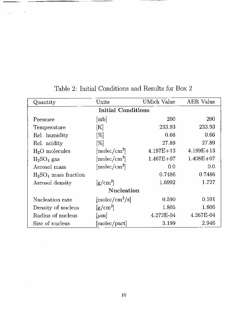
Table 2: Initial Conditions and Results for Box 2
Quantity Units UMich Value AER Value
Initial Conditions
Pressure
Temperature
Rel. humidity
Rel. acidity
H20 molecules
H2SO4 gas
Aerosol mass
H2SO4 mass fraction
Aerosol density
Nucleation rate
Density of nucleus
Radius of nucleus
Size of nucleus
[mb] 200
[K] 233.93
[%] 0.66
[%] 27.89
[molec/cm 3] 4.197E+ 13
[molec/cm 3] 1.407E+07
[molec/cm 3] 0.0
0.7486
[g/cm a] 1.6992
Nucleation
[molec/cm3/s] 0.590
[g/cm a] 1.805
[#m] 4.272E-04
[molec/part] 3.199
200
233.93
0.66
27.89
4.199E+13
1.408E+07
0.0
0.7486
1.727
0.591
1.806
4.267E-04
2.946
10

Table 3: Initial Conditions and Results for Box 3
Quantity Units UMich Value AER Value
Pressure
Temperature
Rel. humidity
Rel. acidity
H20 molecules
H2SO4 gasAerosol mass
Aerosol number
Aerosol avg. radius
H2SO4 mass fraction
Aerosol density
Nucleation rate
Density of nucleus
Radius of nucleus
Size of nucleus
H2SO4 saturation
Mean free path
H2SO4 gas diff. coeff.
Condensation rate
Particle velocity
Coag. Kernel
Number Change
Initial Conditions
[mb] 500
[K] 208.12
[%] 6.366
[%] 100
[molec/cm 3] 2.206E+ 13
[molec/cm 3] 2.603E+05
[molec/cm 3] 3.850E+07
[cm -3] 8.503
[#m] 5.670E-02
0.6168
[g/cm 3] 1.541
Nucleation
[molec/cm3/s] 6.102E-08
[g/cm 3] 1.7905
[,urn] 3.064E-04
[molec/part] 1.032
Condensation
[molec/cm3] 3.056E-03
[cm] 3.328E-05
[cm2/s] 9.119E-02
[molec/cm3/s] 7.1213
Coagulation
[cm/s] 7.823
[cm 3] 1.137E-9
[cm -3 s -1] -8.224E-8
500
208.12
6.366
100
2.206E+13
2.603E+05
3.851E+07
8.259
5.701E-02
0.6168
1.587
6.102E-08
1.766
3.061E-04
1.030
3.051E-03
3.327E-06
9.124E-02
3.659
7.707
1.301E-09
-9.121E-08
11

Table 4 Initial Conditions and Results for Box 4
Quantity Units UMich Value AER Value
Pressure
Temperature
Rel. humidity
Rel. acidity
H20 molecules
H2SO4 gas
Aerosol mass
Aerosol number
Aerosol avg. radius
H2SO4 mass fraction
Aerosol density
Nucleation rate
Density of nucleus
Radius of nucleus
Size of nucleus
H2SO4 saturation
Mean free path
H2SO_ gas diff. coeff.
Condensation rate
Particle velocity
Coag. Kernel
Number Change
Initial Conditions
[rob] 200
[K] 218.05
[%] 95.43
[%] 100
[molec/cm 3] 1.110E+ 15
[molec/cm 3] 2.293E+06
[molec / cm 3] 2.484E+08
[cm -a] 411.08
[#m] 5.700E-02
0.1163
[g/cm a] 1.091
Nucleation
[lnolec/cm 3/s] 3.688
[g/cm 3] 1.650[ttm] 3.609E-04
[molec/part] 1.346
Condensation
[molec/cm 3] 1.458E- 11
[cm] 8.718E-06
[cm2/s] 0.244
[molec/cma/s] 4432
Coagulation
[cm/s] 9.517
[cm 3] 2.122E-9
[tin -a S-1] -3.587E-4
200
218.05
95.43
100
1.110E+15
2.293E+06
2.485E+08
402.99
5.701E-02
0.1163
1.113
3.689
1.636
3.606E-4
1.343
1.457E-11
8.715E-06
0.245
2431
9.419
2.408E-09
-3.678E-04
12

Box 1 no gas sourceAerosol Mass Aerosol Number Concentration
14
6o0 /_s S
-_ 40o / / ---- uMxcH fi8
I / ---- UMICH (_=0.04) . =
11 I / _ Arg t -_ 6- II I/ ---- AER (0_--'0.04) / 4
0 I0 5 10 15 20 25 30 0 0 5 10 15 20 25 30
time [mini time [mini
__ Nucleation Rate (lOs averages) 2s[/i°ndensati°nRate(lOsaverage_i_ r , , , .... I .... ",02 ,-., 20 ]
loo.1 '°lAt
0.0 0 5 101L=_=I====*'I_$ 0 5 10 15
time [minl time [mini
13

Box 2 no gas sourceAerosol Mass Aerosol Number Concentration
14

38.7
38.6
E
38.5
38.4
Box 3 no gas source
Aerosol Mass
0 5 l0 15 20
time [hi
8.6
8.5
8.4
8.3
8.2
Aerosol Number Concentration
i I I I I I I I I I I I I I I I I I I I I I I i
5 10 15 20
time [h]
7
m
8e-08
6e-08
4e-08
2e-08
0e+00
Nucleation Rate (10s averages)
0 5 10 15 20
time [h]
E
Condensation Rate (10s averages)
5 10 15 20
time [h]
15

251
250
r_
E
" 249
248
Box 4 no gas sourceAerosol Mass
UMICH
-_-- UMICH let=0.04)
AER
_--- AER (t_=0.04)
0 3 6 9 12
time [hi
Aerosol Number Concentration
40000
300(X)
20000
100(H)
00 3 6 9 12
time [h]
Nucleation Rate (10s averages)5 5000
4 4000
_ i 2000
1 1000
0 00 3 6 0
time [h]
Condensation Rate (10s averages)
i
3
time [hi
16
lxlO 6
_. lx105r_j
E
0 4* _,,-I,-- lxlO
e-
¢J
0L)
1xlO 3
lxlO 2
Ixl06
1xlO 5
E
©
"_ Ixl04
e-,(D¢Je..o
L)lxl03
IxlO 2
•- I I I I l]
I a I Ill
0.001
ii I I I I l I
| | | I|l
0.001
Box 1 Size Distribution Evolution
........ I ........ I ........ I
AER Model
i I Jill
0.01 0.1
Radius (gm)
........ I ........ I
UMICH Model
0.01 0.1
Radius (_m)
m Initialm I hour
5 hours24 hours
I I I I I IIII
1
I I I I I III I
i_ Initial ]
I hour I5 hours24 hours
i i I I IIII
1
17

10000
1000
10000
1000
Box 2 Size Distribution Evolution
AER Model -- lnilial ]
-- I hour I-- 5 hours-- 24 hours
0.001 0.01 0.1 1
Radius (l-tm)
UMICH Model -- Initial-- ] hour-- 5 hours-- 24 hours
0.001 0.01 0.1 1
Radius (lam)
18

Box 3 Size Distribution Evolution
E
e-,
.o
t.,
1
0.1
©
0.01
0.001 ..... I0.001
100 1 ..... I
lOt--
0.1
¢3
0.01
0.001
...... I ........ I
AER Model
! ! ! ! ! I|| I
-- InitialI hour5 hours24 hours
I I
0.01 0.1
Radius (pm)
I IIII
1
...... I ........ I ........ I ' "
UMICH Model -- Initial
-- 1 hour
-- 5 hours
-- 24 hours
0.001 0.01 0.1 I
Radius (lam)
19

10000
1000
Box 4 Size Distribution Evolution
AER Model Initial I
I hour ]
5 hours
24 hours
0.010.001 0.01 0.1 1
Radius (Bm)
,:iOoli,............., ........, ........,,UMICH Model _ InitialI hour
m 5 hours I
I _ 24 hours I
-loo
i 10
=
0.1
0010.001 0.01 O. 1 1
Radius (lam)
2O