NUS-786/3

Volume 3

FINAL REPORT FOR

MODIFICATIONS OF CODESNUALGAM AND BREMRAD

Volume 3: Statistical Considerations of theMonte Carlo Method

For

NATIONAL AERONAUTICS ANDSPACE ADMINISTRATION

Goddard Space Flight CenterGlenn Dale Road

Greenbelt, Maryland

NASA Contract Number NAS5-11781

By

H. Firstenberg

May 1971

NUS CORPORATION4 Research Place

Rockville, Maryland

ASE FILE

https://ntrs.nasa.gov/search.jsp?R=19720016641 2018-09-07T04:41:40+00:00Z

NUS-786/3

FINAL REPORT FORMODIFICATION OF CODES NUALGAM AND BREMRAD

Volume 3: Statistical Considerations of theMonte Carlo Method

For

NATIONAL AERONAUTICS AND SPACE ADMINISTRATIONGoddard Space Flight Center

Glenn Dale RoadGreenbelt, Maryland

NASA Contract Number NAS5-11781

= By

H. Firstenberg

May 1971

NUS CORPORATION4 Research Place

Rockville, Maryland

TABLE OF CONTENTS

Page

List of Figures ii

List of Tables Hi

1. Introduction ' • 1

2. Statistical Considerations of the Monte Carlo Method 2

2.1 Introduction 2

2.2 General Comments on the Accuracy of the 3

Monte Carlo Method

2.3 The Method of Statistical Weights 5

3. Numerical Estimates of Errors 9

Appendix 1 The Bernoulli Scheme, Binomial Distributions 16

and Bernouli's Law of Large Numbers

Appendix 2 DeMoivre - Laplace Limit Theorem 27

LIST OF FIGURES

Page

Figure 1 Frequency Distribution of Monte Carlo 15

Albedos for 0.662 MeV Photons Incident

on a 10cm x 10cm Cylindrical Aluminum

Transport Medium

ii

LIST OF TABLES

Page

Table 1 Results of Albedo Calculations fo ra Parallel 14

Beam of 0.662 MeV Incident Photons on a

10cm Aluminum Cylinder

iii

1. INTRODUCTION

This present Volume Illof the final report NUS-786 to the National Aeronautics

and Space Administration, Goddard Space Flight Center, was prepared by the

NUS Corporation under contract NAS5-11781.

This volume considers the statistics of the Monte Carlo method relative to

the interpretation of the NUGAM2 and NUGAM3 computer code results. A

numerical experiment using the NUGAM2 code is presented and the results

are statistically interpreted.

Section 2 presents the general theoretical considerations of the Monte Carlo

method. Supporting theory is given in Appendices 1 and 2. Section 3 con-

sists of an example application of the theory.

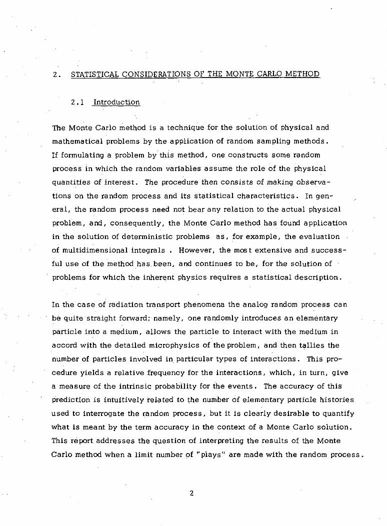
2. STATISTICAL CONSIDERATIONS OF THE MONTE CARLO METHOD

2.1 Introduction

The Monte Carlo method is a technique for the solution of physical and

mathematical problems by the application of random sampling methods.

If formulating a problem by this method, one constructs some random

process in which the random variables assume the role of the physical

quantities of interest. The procedure then consists of making observa-

tions on the random process and its statistical characteristics. In gen-

eral, the random process need not bear any relation to the actual physical

problem, and, consequently, the Monte Carlo method has found application

in the solution of deterministic problems as, for example, the evaluation

of multidimensional integrals . However, the most extensive and success-

ful use of the method has been, and continues to be, for the solution of

problems for which the inherent physics requires a statistical description.

In the case of radiation transport phenomena the analog random process can

be quite straight forward; namely, one randomly introduces an elementary

particle into a medium, allows the particle to interact with the medium in

accord with the detailed microphysics of the problem, and then tallies the

number of particles involved in particular types of interactions. This pro-

cedure yields a relative frequency for the interactions, which, in turn, give

a measure of the intrinsic probability for the events. The accuracy of this

prediction is intuitively related to the number of elementary particle histories

used to interrogate the random process, but it is clearly desirable to quantify

what is meant by the term accuracy in the context of a Monte Carlo solution.

This report addresses the question of interpreting the results of the Monte

Carlo method when a limit number of "plays" are made with the random process

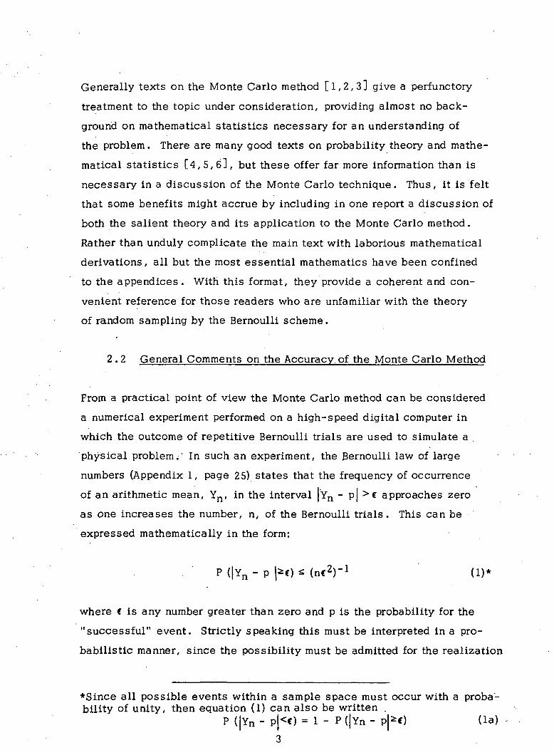
Generally texts on the Monte Carlo method [1 ,2 ,3] give a perfunctory

treatment to the topic under consideration, providing almost no back-

ground on mathematical statistics necessary for an understanding of

the problem. There are many good texts on probability theory and mathe-

matical statistics [4 ,5 ,6 ] , but these offer far more information than is

necessary in a discussion of the Monte Carlo technique. Thus, it is felt

that some benefits might accrue by including in one report a discussion of

both the salient theory and its application to the Monte Carlo method.

Rather than unduly complicate the main text with laborious mathematical

derivations, all but the most essential mathematics have been confined

to the appendices. With this format, they provide a coherent and con-

venient reference for those readers who are unfamiliar with the theory

of random sampling by the Bernoulli scheme.

2 .2 General Comments on the Accuracy of the Monte Carlo Method

From a practical point of view the Monte Carlo method can be considered

a numerical experiment performed on a high-speed digital computer in

which the outcome of repetitive Bernoulli trials are used to simulate a

"physical problem. In such an experiment, the Bernoulli law of large

numbers (Appendix 1, page 25) states that the frequency of occurrence

of an arithmetic mean, Yn, in the interval [Vn - p| >C approaches zero

as one increases the number, n, of the Bernoulli trials. This can be

expressed mathematically in the form:

P (|Yn - p |*c) * (ne2)'1 (1)*

where € is any number greater than zero and p is the probability for the

"successful" event. Strictly speaking this must be interpreted in a pro-

babilistic manner, since the possibility must be admitted for the realization

*Since all possible events within a sample space must occur with a proba-bility of unity, then equation (1) can also be written .

P (|Yn - P|<€) = 1 - P (|Yn - p|*C) (la)3

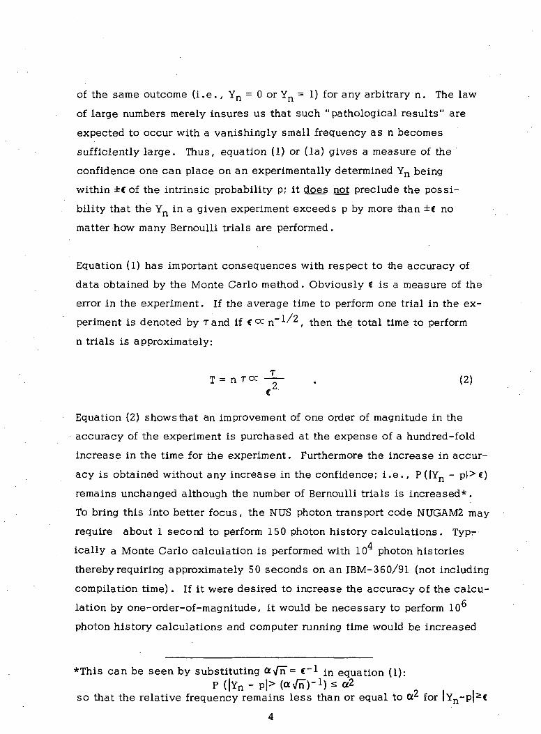
of the same outcome (i.e., Yn = 0 or Yn = 1) for any arbitrary n. The law

of large numbers merely insures us that such "pathological results" are

expected to occur with a vanishingly small frequency as n becomes

sufficiently large. Thus, equation (1) or (la) gives a measure of the

confidence one can place on an experimentally determined Yn being

within ±Cof the intrinsic probability p; it does not preclude the possi-

bility that the Yn in a given experiment exceeds p by more than ±€ no

matter how many Bernoulli trials are performed.

Equation (1) has important consequences with respect to the accuracy of

data obtained by the Monte Carlo method. Obviously € is a measure of the

error in the experiment. If the average time to perform one trial in the ex-

periment is denoted by Tand if € °c n"1/^, then the total time to perform

n trials is approximately:

T = n r cc-I- (2)r

Equation (2) shows that an improvement of one order of magnitude in the

accuracy of the experiment is purchased at the expense of a hundred-fold

increase in the time for the experiment. Furthermore the increase in accur-

acy is obtained without any increase in the confidence; i.e., P(lYn - p l > € )

remains unchanged although the number of Bernoulli trials is increased*.

To bring this into better focus, the NUS photon transport code NUGAM2 may

require about 1 second to perform 150 photon history calculations. Typ-

ically a Monte Carlo calculation is performed with 10 photon histories

thereby requiring approximately 50 seconds on an IBM-360/91 (not including

compilation time). If it were desired to increase the accuracy of the calcu-

lation by one-order-of-magnitude, it would be necessary to perform 10°

photon history calculations and computer running time would be increased

*This can be seen by substituting a/n~ = e~l in equation (1):P (|Yn- p |>(o^)- l )so2

so that the relative frequency remains less than or equal to a2 for |Yn-p|^€

to about 1.4 hours.

The absolute error in a calculation is less meaningful than the relative

error; i.e.,

(3)

In terms of the relative error €r, the number of trials required to achieve

a given accuracy will vary inversely as the "intrinsic probability for the

event" p. Obviously, a direct modeling of the problem becomes imprac-

ticable when the event being investigated has a small probability thus, one

must be willing to accept less accuracy in the result or change the strategy of the

experiment to enhance the probability of success. For exam pie, if the probability for

the transmission of photons through a shield is of the order of 10"^, then a

modeling of "physical trajectories" for 10^ photons would be required for

about 100 photons to penetrate the shield. A large relative error can be

expected for the number of photons that penetrate the shield, and informa-

tion on the direction and energy of the emerging photons would be less

accurately known.

2.3 The Method of Statistical Weights

A procedure for circumventing the above metioned difficulties is to discard

the modeling of the physical trajectory and to introduce the artifice of statis-

tical weights. This technique increases the probability for the successful

outcome in an experiment by application of some statistical weight which

permits the continuance of the trajectory after each event rather than

terminate the history by an unsuccessful event. Thus, if the probability for

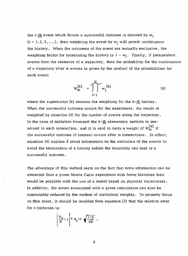
the i-th event which favors a successful outcome is denoted by w^

(i = 1 , 2 , 3 , . . . ) , then weighting the event by wi will permit continuance

the history. When the outcomes of the event are mutually exclusive, the

weighting factor for terminating the history is 1 - w^. Finally, if independent

events form the elements of a trajectory, then the probability for the continuance

of a trajectory after m events is given by the product of the probabilities for

each event:

m"""" fM

<4>

i=l

where the superscript (k) denotes the weighting for the k-th history-

When the successful outcome occurs for the experiment, the result is

weighted by equation (4) for the number of events along the trajectory.

In the case of radiation transport the k-th elementary particle is pre-(k)served in each interaction, and it is said to carry a weight of Wm if

the successful outcome of interest occurs after m interactions. In effect,

equation (4) applies a priori information on the statistics of the events to

avoid the termination of a history before the trajectory can lead to a

successful outcome. .

The advantage of this method rests on the fact that more information can be

extracted from a given Monte Carlo experiment with fewer histories than

would be possible with the use of a model based on physical trajectories.

In addition, the errors associated with a given calculation can also be

appreciably reduced by the method of statistical weights. To properly focus

on this point, it should be recalled from equation (3) that the relative error

for n histories is:

<€ cc JHF.r 1 np

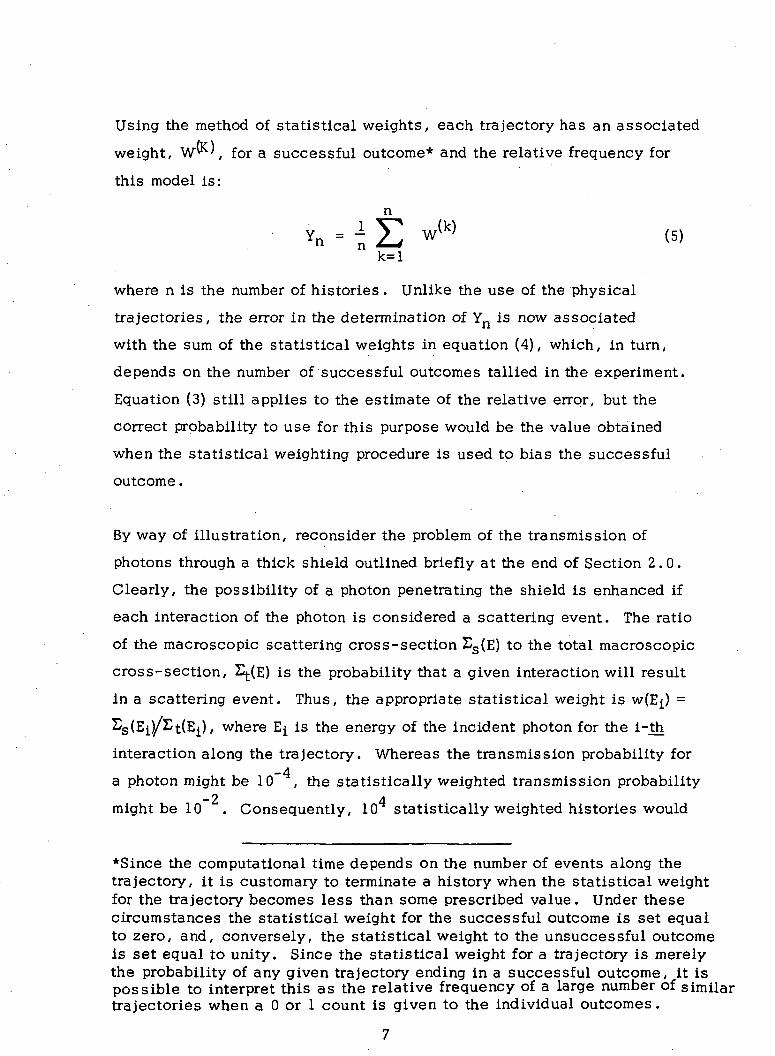
Using the method of statistical weights, each trajectory has an associated

weight, W^, for a successful outcome* and the relative frequency for

this model is:

11

'n • -i Ewhere n is the number of histories. Unlike the use of the physical

trajectories, the error in the determination of Yn is now associated

with the sum of the statistical weights in equation (4), which, in turn,

depends on the number of successful outcomes tallied in the experiment.

Equation (3) still applies to the estimate of the relative error, but the

correct probability to use for this purpose would be the value obtained

when the statistical weighting procedure is used to bias the successful

outcome.

By way of illustration, reconsider the problem of the transmission of

photons through a thick shield outlined briefly at the end of Section 2 . 0 .

Clearly, the possibility of a photon penetrating the shield is enhanced if

each interaction of the photon is considered a scattering event. The ratio

of the macroscopic scattering cross-section SS(E) to the total macroscopic

cross-section, £t(E) is the probability that a given interaction will result

in a scattering event. Thus, the appropriate statistical weight is w(Ei) =

£s(Ei)/£t(Ei), where EI is the energy of the incident photon for the i-th

interaction along the trajectory. Whereas the transmission probability for-4a photon might be 10 , the statistically weighted transmission probability

— 9 A

might be 10 . Consequently, 10 statistically weighted histories would

*Since the computational time depends on the number of events along thetrajectory, it is customary to terminate a history when the statistical weightfor the trajectory becomes less than some prescribed value. Under thesecircumstances the statistical weight for the successful outcome is set equalto zero, and, conversely, the statistical weight to the unsuccessful outcomeis set equal to unity. Since the statistical weight for a trajectory is merelythe probability of any given trajectory ending in a successful outcome, it ispossible to interpret this as the relative frequency of a large number of similartrajectories when a 0 or 1 count is given to the individual outcomes.

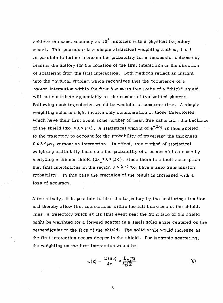
achieve the same accuracy as 10" histories with a physical trajectory

model. This procedure is a simple statistical weighting method, but it

is possible to further increase the probability for a successful outcome by

biasing the history for the location of the first interaction or the direction

of scattering from the first interaction. Both methods reflect an insight

into the physical problem which recognizes that the occurrence of a

photon interaction within the first few mean free paths of a "thick" shield

will not contribute appreciably to the number of transmitted photons.

Following such trajectories would be wasteful of computer time. A simple

weighting scheme might involve only consideration of those trajectories

which have their first event some number of mean free paths from the backface

of the shield (Mxj ^X^ M£) . A statistical weight of e~^xl is then applied

to the trajectory to account for the probability of traversing the thickness

0 ^\<Mx-| without an interaction. In effect, this method of statistical

weighting artificially increases the probability of a successful outcome by

analyzing a thinner shield (jix^X^ M ^ ) / since there is a tacit assumption

that first interactions in the region 0 ^ X < Mx^ have a zero transmission

probability. In this case the precision of the result is increased with a

loss of accuracy.

Alternatively, it is possible to bias the trajectory by the scattering direction

and thereby allow first interactions within the full thickness of the shield.

Thus, a trajectory which at its first event near the front face of the shield

might be weighted for a forward scatter in a small solid angle centered on the

perpendicular to the face of the shield. The solid angle would increase as

the first interaction occurs deeper in the shield. For isotropic scattering,

the weighting on the first interaction would be

<«

and subsequent weights applied to events along the trajectory would be

w(Ei) = Ss(Ei)/St(Ei) , Ei* E . If O (Mx) = 4ff for X * Hx, then this technique

for statistical weighting is an improved version of confining first inter-

actions to MX-^ < X < M-k/since a finite transmission probability is allowed

first interactions in 0 ^ X <

Either of these approaches to the solution of photon transmission through

a thick shield conserves histories by increasing the likelihood of a successful

outcome, albeit there might be some small systematic error introduced by

the biasing scheme. The second approach is obviously more desirable, since

the systematic error should be smaller. Equally clear from this illustrative

example is the fact that the optimization of a Monte Carlo solution rests on

the ingenuity of the programmer for the selection of a statistical weighting

scheme which increases the probability for a successful outcome of interest

without a sacrifice in accuracy.

3. NUMERICAL ESTIMATES OF ERRORS

The error introduced in the Monte Carlo method was considered in general

terms in Sections 2.0 and 3.0. In this section the errors in an actual

Monte Carlo calculation are considered for the albedo of a parallel beam

of 0.662 MeV photons incident on a cylinder of aluminum (R = H = 10cm) .

Specifically, .this section will consider the interpretation of the errors

associated with experimental results.

By way of a preliminary introduction, the usual statement of the error in

a Monte Carlo calculation is usually assumed to be taken as n"1/^,

where n is the number of histories . This can be understood in terms

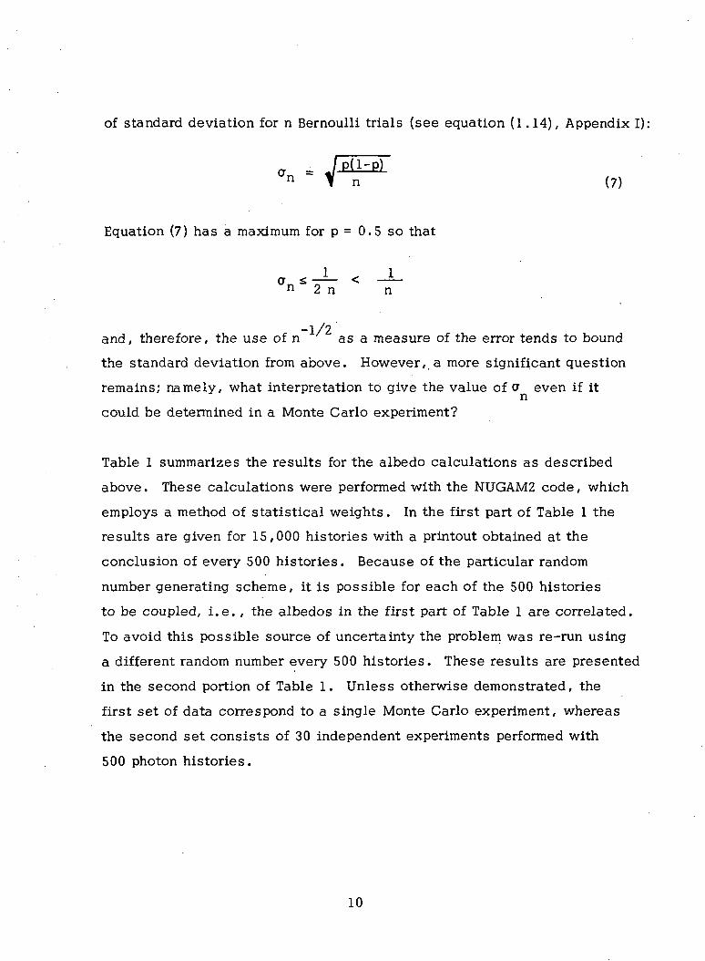
of standard deviation for n Bernoulli trials (see equation (1.14), Appendix I):

- - -^Equation (7) has a maximum for p = 0.5 so that

n 2 n n

-1/2and, therefore, the use of n as a measure of the error tends to bound

the standard deviation from above. However, a more significant question

remains; namely, what interpretation to give the value of cr even if itncould be determined in a Monte Carlo experiment?

Table 1 summarizes the results for the albedo calculations as described

above. These calculations were performed with the NUGAM2 code, which

employs a method of statistical weights. In the first part of Table 1 the

results are given for 15,000 histories with a printout obtained at the

conclusion of every 500 histories. Because of the particular random

number generating scheme, it is possible for each of the 500 histories

to be coupled, i.e. , the albedos in the first part of Table 1 are correlated.

To avoid this possible source of uncertainty the problem was re-run using

a different random number every 500 histories. These results are presented

in the second portion of Table 1. Unless otherwise demonstrated, the

first set of data correspond to a single Monte Carlo experiment, whereas

the second set consists of 30 independent experiments performed with

500 photon histories.

10

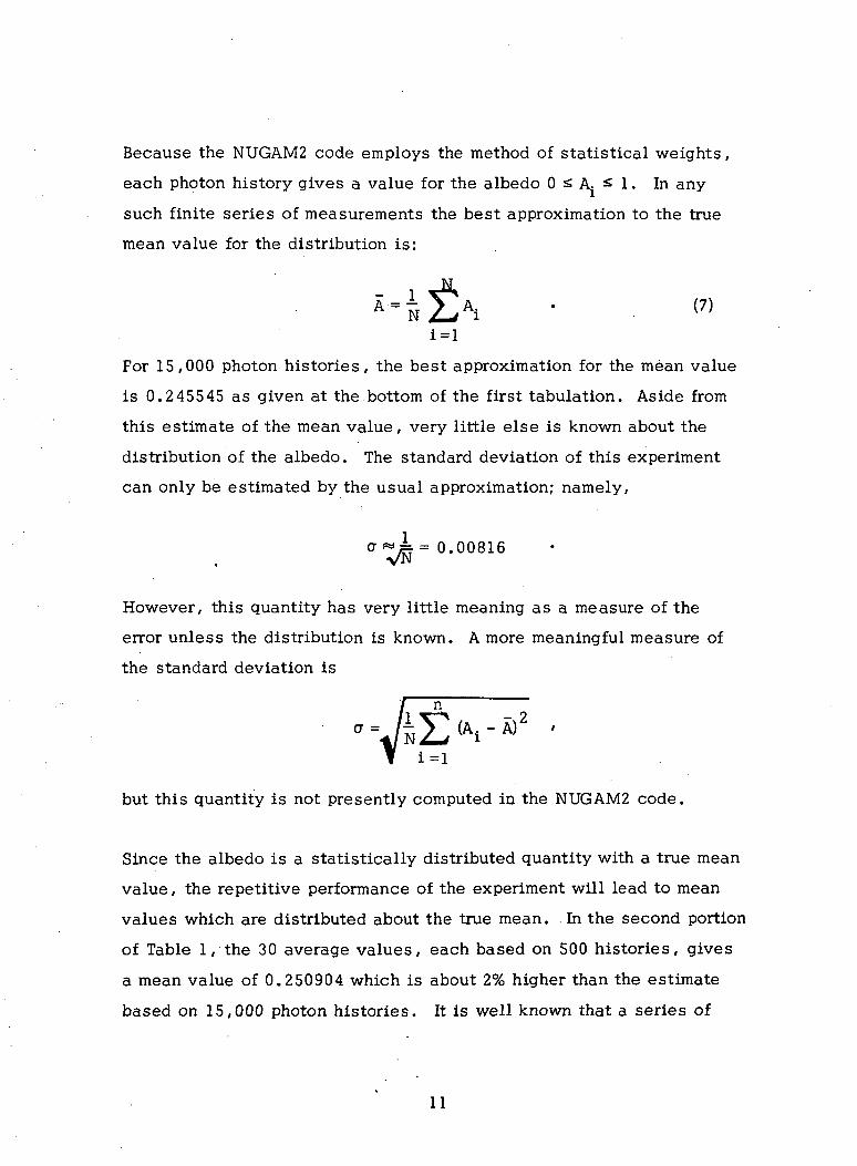
Because the NUGAM2 code employs the method of statistical weights,

each photon history gives a value for the albedo 0 ^ A. ^ 1. In any

such finite series of measurements the best approximation to the true

mean value for the distribution is:

i > :*. • m

For 15,000 photon histories, the best approximation for the mean value

is 0.245545 as given at the bottom of the first tabulation. Aside from

this estimate of the mean value, very little else is known about the

distribution of the albedo. The standard deviation of this experiment

can only be estimated by the usual approximation; namely,

a ~= = 0.00816

However, this quantity has very little meaning as a measure of the

error unless the distribution is known. A more meaningful measure of

the standard deviation is

1=1

but this quantity is not presently computed in the NUGAM2 code.

Since the albedo is a statistically distributed quantity with a true mean

value, the repetitive performance of the experiment will lead to mean

values which are distributed about the true mean. .In the second portion

of Table 1, the 30 average values, each based on 500 histories, gives

a mean value of 0.250904 which is about 2% higher than the estimate

based on 15,000 photon histories. It is well known that a series of

11

k mean values, each based on n observations, will tend to exhibit a

normal distribution about their grand average. Appendix 2 gives the

mathematical derivation for the normal distribution as a limiting form of

the binomial distribution. Although the DeMoivre-Laplace Limit Theorem

is a more restrictive case of the Central Limit Theorem it is sufficient

for the present purpose. Suffice it to state that the distribution of the

mean values tends to be normal irrespective of the distribution from

which the observations are made. Thus, it is possible to obtain an

estimate of the true mean value and also an estimate of the error.

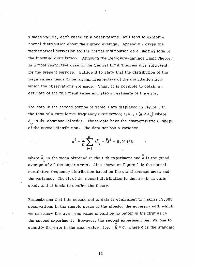
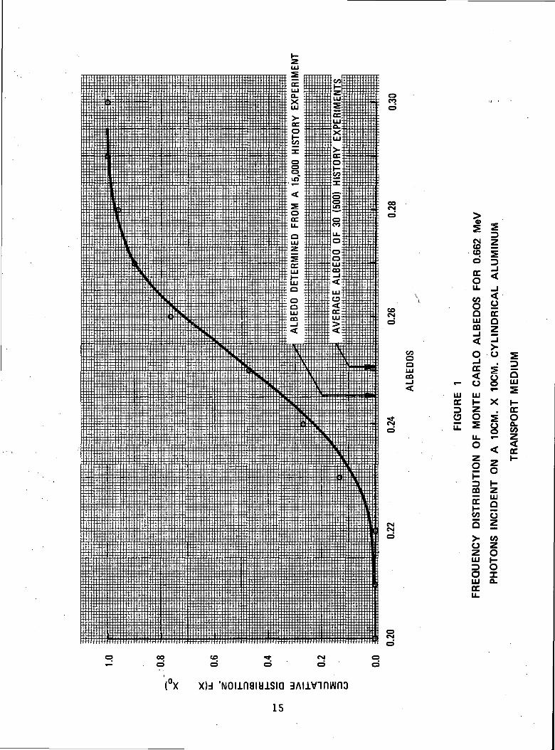
The data in the second portion of Table 1 are displayed in Figure 1 in

the form of a cumulative frequency distribution; i.e. , F(A < A ) where

A is the abscissa (albedo). These data have the characteristic S-shapeoof the normal distribution. The data set has a variance

na2 =^ \^ (A. - A)2 = 0.01438 . ,

1=1

where A. is the mean obtained in the 1-th experiment and A is the grand

average of all the experiments. Also shown on Figure 1 is the normal

cumulative frequency distribution based on the grand average mean and

the variance. The fit of the normal distribution to these data is quite

good, and it tends to confirm the theory.

Remembering that this second set of data is equivalent to making 15,000

observations in the sample space of the albedo, the accuracy with which

we can know the true mean value should be no better in the first as in

the second experiment. However, the second experiment permits one to

quantify the error in the mean value, i.e. , A ± cr, where cr is the standard

12

deviation for the distribution of mean values. Since the distribution of

mean values will approximate a normal distribution, it is possible to

state that the probability is 68% for the true mean to be within ± a of

the grand average mean. The best estimate of the mean value from 15,000

photon histories (data set #1, Table 1) is in agreement with this

interpretation.

13

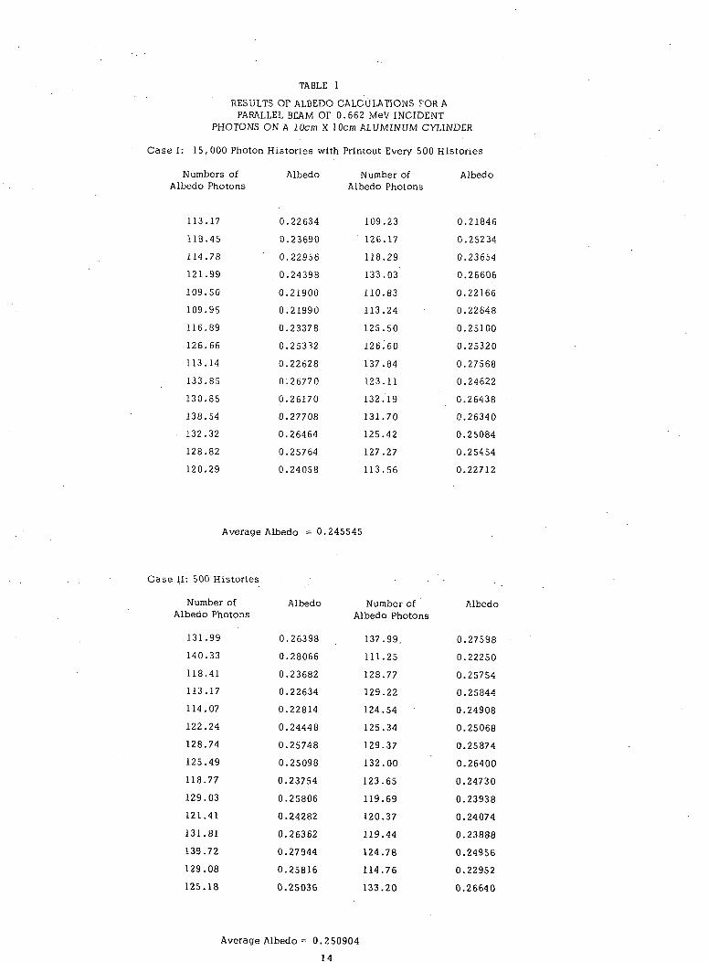
TABLE 1

RESULTS OF ALBEDO CALCULATIONS FOR APARALLEL BEAM OF 0 .662 MeV INCIDENT

PHOTONS ON A 10cm X 10cm ALUMINUM CYLINDER

Case I: 15,000 Photon Histories with Printout Every 500 Histories

Albedo

0.21846

0.25234

0.23654

0.26606

0.22166

0.22648

0.25100

0.25320

0.27568

0.24622

0.26438

0.26340

0.25084

0.25454

0.22712

Numbers ofAlbedo Photons

113.17

118.45

114.78

121.99

109.50

109.95

116.89

126.66

113.14

133.85

130.85

138.54

132.32

128.82

120.29

Average

Case II: 500 Histories

Number ofAlbedo Photons

131.99

140.33

118.41

113.17

114.07

122.24

128.74

125.49

118.77

129.03

121.41

131.81

139.72

129.08

125.18

Albedo

0.22634

0.23690

' 0 .22956

. 0.24398

0.21900

0.21990

0.23378

0.25332

0.22628

0126770

0.26170

0.27708

0.26464

0 .25764

0.24058

Albedo = 0

Albedo

0.26398

0.28066

0.23682

0.22634

0.22814

0.24448

0.25748

0.25098

0.23754

0.25806

0.24282

0.26362

0.27944

0.25816

0.25036

Number ofAlbedo Photons

109.23

126.17

118.29

133.03

110.83

113.24.

125.50

126^60

137.84

123.11

132.19

131.70

125.42

127.27

113.56

.245545

Number ofAlbedo Photons

137.99.

111.25

128.77

129.22

124.54

125.34

129.37

132.00

123.65

119.69

120.37

119.44

124.78

114.76

133.20

Albedo

0.27598

0.22250

0.25754

0.25844

0.24908

0.25068

0.25874

0.26400

0.24730

0.23938

0.24074

0.23888

0.24956

0.22952

0.26640

Average Albedo = 0.250904

14

00CM

s Is sO D

<= <O ̂

COOJ

UCC

LU QZCO

COoLUCO

o o5 s2 £

LU LUCC h-

o oLU S

DQLU

DCO0.V)

CMCM

2 §

— LU£ Q

O Z

& 2z oLU f-

§ §LU O.CC

3Aiivinwno

15

APPEND K 1

THE BERNOULLI SCHEME, BINOMIAL DISTRIBUTIONS

AND BERNOULLI'S LAW OF LARGE NUMBERS

16

Appendix 1: The Bernoulli Scheme, Binomial Distributions and

Bernoulli's Law of Large Numbers.

Most discussions on the accuracy of the Monte Carlo method start

from a statement of the binomial distribution:

p" =

which gives the probability of "exactly" m successful outcomes in

n random experiments. Very little discussion is given to the under-

lying principles of the binomial distribution, which, more often

than not, must be weened from texts on probability theory and

mathematical statistics . For this reason it is felt that many readers

might benefit from a somewhat pedagogical, but unified, treatment

of the subject starting from the concept of the Bernoulli scheme of

sampling and carrying the development through to the accuracy of

the Monte Carlo method and its principal features.

The simplest case of a random event is one for which there are only

two possible outcomes, the event A and the complement of A. This

situation might be abstracted as a sample space consisting of the

events "zero", which we define as an unsuccessful event, and

"one", which we define as a successful event. This "zero-one"

sample space has numerous realizations, some examples of which are

the toss of a coin ("heads" or "tails"), the position of a switch ("on"

or "off") , the random selection of a binary digit ("0" or " 1"), Russian

roulette ("loaded" or "unloaded" chamber), etc. For purposes of this

presentation, it will be assumed that the outcome of any given ex-

periment does not depend on the previous results obtained so that the

17

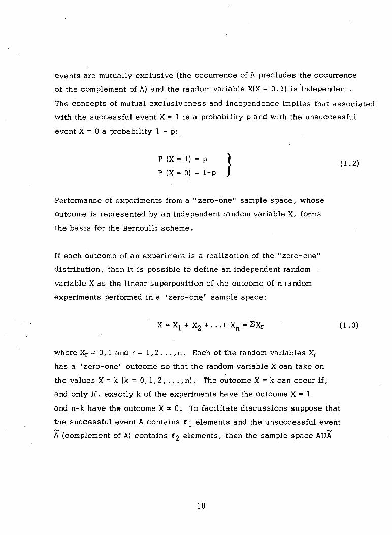
events are mutually exclusive (the occurrence of A precludes the occurrence

of the complement of A) and the random variable X(X = 0, 1) is independent.

The concepts of mutual exclusiveness and independence implies that associated

with the successful event X = 1 is a probability p and with the unsuccessful

event X = 0 a probability 1 - p:

P (X= 0) = 1-p

Performance of experiments from a "zero-one" sample space, whose

outcome is represented by an independent random variable X, forms

the basis for the Bernoulli scheme.

If each outcome of an experiment is a realization of the "zero-one"

distribution, then it is possible to define an independent random

variable X as the linear superposition of the outcome of n random

experiments performed in a "zero-one" sample space:

X = Xx + X2 +• ..+ Xn = Sxr (1.3)

where Xr = 0,1 and r = 1, 2 . .., n. Each of the random variables Xr

has a "zero-one" outcome so that the random variable X can take on

the values X = k (k = 0,1, 2, ..., n). The outcome X = k can occur if,

and only if, exactly k of the experiments have the outcome X = 1

and n-k have the outcome X = 0. To facilitate discussions suppose that

the successful event A contains €} elements and the unsuccessful event

A (complement of A) contains €2 elements, then the sample space AUA

18

contains e = €j + c2 elements*. If each of these elements are equally

likely to occur (a true die), then the I priori probability of the event As\s

and A would be p= f i/C and l - p = *2/*' respectively. If the experiment

is performed n times, then the number of ways to arrive at the event AJc ~ n—kexactly k times is €v and at the event A exactly n-k times is €' .

Consequently, the number of ways one can obtain exactly k successes andk n-kn-k failures is C1 €2 • Obviously, the number of possible outcomes in n

random experiments is €n. As yet nothing has been said about the ordering

of successful or unsuccessful outcomes. If the successful outcomes could

be distinguished; that is one could somehow "tag" the{l' s}(the set lj ,

j = 1, 2 .. ., k) in order to differentiate between X = 1^ and X = lj, then the

number of different ways .of arriving at exactly k successes and n-k failures

is:

n(n-l). ..(n-k+1) = n<

(n-k)!

The number of possible ways of arranging the set 1- is given by

k(k- l ) . . . 1 = k!, and, therefore, the number of indistinguishable ways

of arranging exactly k successes and n-k failures in n random experiments

is:

*A realization of such a sample space would be the possible outcomes fromthe throw of a die. The six faces of a die are numbered 1 through 6. If theoutcome 1 or 2 is considered a successful outcome (the event A) and 3 , 4 , 5and 6 is considered an unsuccessful outcome (the event A), then C^ = 2;€2 = 4 and € = € i + C 2 = 6. The random variable X = 1 is assigned whenthe die shows a 1 or 2, and X = 0 is assigned when the die shows a3 , 4 , 5 or 6.

19

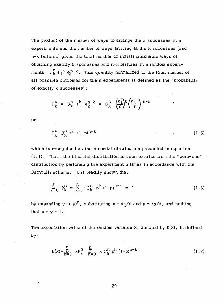
The product of the number of ways to arrange the k successes in n

experiments and the number of ways arriving at the k successes (and

n-k failures) gives the total number of indistinguishable ways of

obtaining exactly k successes and n-k failures in n random experi-

ments: c£ €j C2n~k. This quantity normalized to the total number of

all possible outcomes for the n experiments is defined as the "probability

of exactly k successes":

pn _ n k -n-k _ rn / C l \ k / € 2 \ n-IFk ~ uk cl €2 '" uk

or

(1.5)

which is recognized as the binomial distribution presented in equation

(1.1). Thus, the binomial distribution is seen to arise from the "zero-one"

distribution by performing the experiment n times in accordance with the

Bernoulli scheme . It is readily shown that:

Jo ^ - L c£ >k <i-'"n"k • 1 < ' - 6

by expanding (x + y)n, substituting x = €]/€ and y = €2/*, -and nothing

that x + y = 1 .

The expectation value of the random variable X, denoted by E(X) , is defined

by:

k Cn pk (l-p)n~k (1.7)

20

Since:

k rn nk M-nln~k -S _ k (n!) _ nkk C k p (1 p) -]T=0 k! (n-k)! p

= 8 - - - pk(l-p)n-k

lc=0 (k-1)! (n-k)! p u w

--"ȣ " 1"*=0 I \ (m~t)! H ^ H;

then equations (1.6) and (1.7)give:

E(X) = np . (1.8)

Similarly, the expectation value of the random variable X , denoted by

E(X2), is defined by:

E(X2) =£ k2 G£ pk (l-p)n~k , (1.9)

which can be shown to reduce to:

, E(X2) = np + n(n-l) p2 ' , (1.10)

9following the procedure outlined above. The second central moment D(X )

is obtained from equations (1.8) and (1.10):

D(X2) = E(X2) -E 2(X) = np( l -p) . (1.11)

If instead of the random variable X one defines a new random variable Y:

Y - - -n

21

where Y can take on the values

"' n ' n'"" n ' *

then the probability of Y = k/n is equal to the probability of exactly k

successes in n random experiments:

P(Y" n) = P k = Ckpk(1"p)n"k ' (1'12)

Following the procedures outlined above, it can be shown that the

expectation value of Y is:

E(Y) = ^E(X) = p (1.13)

and the second central moment (or variance) of Y is:

(1.14)

Before deriving Bernoulli's Law of Large Numbers, it is necessary to

develop first the so-called Chebychev inequality. To this end, define

the random variable:

0 = [ Y - E ( Y ) ] 2 = ^ 2 CX-E(X) ] 2 , (1.15)

then

= -2 EJ[X - E(X)]2} = ̂ 2 [E(X2) - 2XE(X) + E2(X)]

22

and from equation (1.14):

E(0) = ^2 {E(X2) - E2(X)| = cr2 . (1.16)

If a random variable can take on only non-negative values, then

nE(X) = £_ kp" * m P

K—ITl JC

m=}=0

or

m

where

nP(k2=m)= ,L P,n

k=m km>0

and represents the probability of m or more successes in n random

experiments. Since the random variable 0, defined by equation (1.15),

satisfies the requirements leading to equation (1. 17) we can immediately

write

m

defining m = a2a2:

P(<^a2m2)

or, recognizing that $feofiai is equivalent to |0 j ^oto, then

p(|0| ^ a a ) s ^-2 (1.18)a

23

where

Equation (1.18) is the Chebychev inequality.

Making a slight change in nomenclature, the random variable $n is defined

by .

where the subscript n is used to denote the results obtained from n

random experiments. Consequently, the Chebychev inequality gives:

From equation (1 . 14):

n

and letting

p(l-p)where €<0, then

n€2 (1.19)*

* Since 0 z p£ 1 , then the expression p(l-p) has a maximum value atP = 1/2; that is

p(l-p) * 1/4 * lwhich is used in equation (1.19)

24

Equation (1.19) is the mathematical statement of the "Bernoulli Law of

Large Numbers." In effect, it requires that for every C> 0

Lim p( j/ * e) =0 . • . (1.20)*

which is the condition for the sequence |$ } to be "stochastically convergent

to zero." The concept of stochastic convergence to zero implies that the pro-

bability of the event $n ^ e tends to zero as n-*00.

An interpretation of the Bernoulli Law of Large Numbers is important in

understanding the statistics of the Monte Carlo Method, since it relates

the accuracy of the calculation to the number of histories used in the

calculations. From equations (1.13) and (1.15), the Bernoulli Law of

Large Numbers can be expressed in the form:

The sequence JYm}represents the normalized values of the random variable

Xn possible in n random experiments:

Xn) „ 1 2 n-1m l m m " n

when the n experiments are conducted according to the Bernoulli scheme

(ie, the possible outcomes of n Bernoulli trials). The sequence {Yn-p|

merely centers the sequence {Yn} relative to the expectation value of

Yn;ie., E(Yn) = p. Thus, equation (1.19) relates the frequency of

observing values of |Yn-p| ^ C as the number of Bernoulli trials is

increased. For example, taking C= 0.1 then equation (1.19) becomes

*Equation (1.20) is obtained in the straightforward manner from equation

(1.19). Since P( |0n| ^ e) * 0 , then

Lim P( |4u| * €) £ Lim ~? = 0

which can be satisfied if, and only if P( |^| s € )=0as n ->^° provided the

limit exists25

P ( | Y n - p |

so that in 102 experiments, P( JYn-p ^0 .1 ) £ 1.0; in 103 experiments,

P( Yn-p| s 0.1) ^ 0.1; and in 105 experiments, P( Yn-p| * 0. l)s 0. 001.

Consequently, as the number of Bernoulli trials is increased (with constant

€), the frequency of observing JYn-p| ^ € decreases toward zero (stochastically

converges to zero). The value of c can be interpreted as the error associated

with the determination of expectation value of JYn} from n Bernoulli trials.

In the above example, the Bernoulli Law of Large Numbers suggests a large

uncertainty in the determination of p from only 100 experiments while for

lO^^experiments the frequency of observing experimental values for{Yn }

in the range p ± 0.1 is better than 0.999.

If, instead of holding € constant, one allows C to approach zero as n

increases without bound, then the probability that the observed frequency

of the (successful) event A differs little from pis close to unity. The rate

of convergency is slow since C cannot decrease any faster than n~* '^ for

stochastic convergency to zero; ie., one must increase the number of

Bernoulli trials by more than two-orders-of-magnitude to achieve a reduction

in the error by one-order-of-magnitude. This imposes a practical limitation

on the Monte Carlo method, because the computational time varies directly

as the number of Bernoulli trials (histories or trajectories) used in the cal-

culation: t « n .

26

APPENDIX 2

DeMOIVRE - LAPLACE LIMIT THEOREM

27

Appendix 2: DeMoivre - Laplace Limit Theorem

In the previous discussion of the Bernoulli Law of Large Numbers [Appendix

1, equation (1.21)] it was implied that stochastic convergence existed for

all values of the argument:

Lim P( Yn-p * €) = 0n — fr00

for each € > 0 . However, if ^->0 as n-»°°is then one is presented with a

difficulty. Since

then one is interested in those cases where n-»°° and Xn(=k)-*00 in such a

manner that

Mk = k - npn n 0. (2.1)

For reasons to become obvious below, we will require that n °° and k °°

in such a manner that

2

-S- - »0 (2 .2 )n

which also contains the condition of equation (2.1);

The binomial distribution [Appendix 1, euqation (1.5)1 can be cast into the

form:

-—2ffk(n-k)J

28

when Stirling's formula

ml ~V2lT mm+2 e'm

is used to approximate the factorial terms of C, . In equation (2.3)

q = 1-p and the sign ~denotes that the ratio of the two sides tends to

unity. Introducing the variable /J^ into equation (2.3)

0 -ftand using the Taylor representation

Y2 y3 Y4

In (1 + X) = 1 + X -- + - - - ±

for the second term of the right-hand side gives

+.. (2.4)-In Pn~ 1/2 In [JZirnpqf l +^Vl-L \ nP/\ np

Subject to the condition of equation (2 .2 ) , in the limit of large n, equation

(2.4) takes on the asymptotic form: ,

which is recognized as the "normal" distribution function. Defining the

standardized random number:

= k - np

then the equation (2 .5) can be cast in the form:

(2.6)

29

-1/2where h= (mpq) . The conditions expressed by equations (2.1) and

(2.2) can be expressed in the form

M3

as n- °°. The probability of a £ ^ ^ /3 is:

+ . . . + P + P (2 .7 )

so fiat if equation (2 . 6) is satisfied for all k (k = a, a + 1 , . . . , jS ) in the

interval/equations (2 .6) and (2 .7) give

0(Xa + 1)+.. .+0(X j S)L (2.8)

To digress for a moment consider the area under the curve y = f(X) in the

interval xk - l/2h =£ xs xk + l/2h, then from the first mean value theorem:

L f(X) dX = hf (£k); xk - l/2h < 4k <xk + l/2h

From this it is clear that the right hand member of equation (2 .6) can be

represented as an integral of the function:

d *(X) = 0 (X) dX

over the interval x]c_1/2 ^ xk+i/2* • Further/ if h X^ - 0 (h=a , a + 1,...",)

for all a s. xn £ /3, then equation (2 .8) can be represented to some order of

approximation, by the integral over the interval a-1/2 ^ x£ /3+ 1/2. The

questing remains as to the "goodness" of this approximation as a fit to

h0(xk).

* From the definition of xk;

xk ± i/2h = [k-np] ± l/2h = h[(k ± 1/2) -np]Hxk ± 1/2.

30

In the interval xk - l/2h * x £ xk + l/2h:

* (xk + 1/2) - *( xk - 1/2) = J 0 {x)dx = h0(£k)

or, from equation (2.5)

exp. 1/2) - *(X - 1/2 ) = (2.9)

Since xk - l/2h < €k < xk + l/2h:

l/2h|xk

and

= 1/2 xk) = l/2h(xk - l/4h)^-h [|xkAl/4h|>-C

then equation (2 .9) can be written

"€

1/2) - 4<xk - 1/2)] <h 0 (xk) < ec j*(xk - 1/2)

or, for an arbitrary € > 0

(xk)*(xk+l/2) - *(xk - 1/2)

- 1 < €

since h/X]^ - * 0 a n d h - * 0 a s n-»0. Consequently;

h 0(xk) ~ *(xk+ 1/2) - *(xk - 1/2) = f^^1 2 0 (x)dxxk-l/2

31

and summing over k(k = a , a + 1 , . . . , j8) gives

P«x * Xn *# ~ *(x0 + 1/2) - f' 0W« (2.10)*

which is the DeMoivre-Laplace limit theorem. This limit theorem states

that, to some order of approximation, the probabilities of the binomial

distribution can be estimated by treating the standarized random variable

as "a continuous random variable with a "normal" distribution.

The DeMoivre-Laplace limit theorem is a special case of a more general

limit theorem known as the "Central Limit Theorem" .

The central limit theorem is obeyed by a sequence |xn} if for every & </3:

P ( a < z m < / 3 ) ~ * (/3) - * (a).

This statement of the central limit theorem is formally similar to the

DeMoivre-Laplace limit theorem, but it need not be confined to the

X^ being drawn from a common binomial distribution. The Linderberg-

Levy theorem insures that the central limit theorem holds for every uniformly

bounded sequence |xn} of mutually independent random variables, i.e. ,

I XjJ <A for all n. By this we mean that for every n there are n mutually

independent random variables X, X,, • • . , Xn with prescribed distributions

such that |xk| <A for all k.

* Since xe ± \/i = xk + l/2h and h -* 0 as n -°°, then equation (2.10) can bewritten:

This form of the Demoivre-La place limit theorem is found in the literature,but it is more restrictive than equation (2.10).

32

TELEPHONE (301) 948-7010 CABLE: