Final Report of Special Problem

Stephen Hanks

SWS 6905 Spring-Summer C 11 DE

TITLE

“One dimensional hydraulic analysis of the effect of sea level rise on estuarine salinity”

AUTHOR INFORMATION

Stephen Hanks, Graduate Student, Soil & Water Science Department, University of Florida, Gainesville,

Florida

Correspondence: hanks705@ufl.edu

KEY TERMS

sea level rise; salinity; hydraulic modeling; Caloosahatchee; minimum flows and levels

ABSTRACT

Projections of global climate change over the next century indicate that multiple stresses to coastal

ecosystems are expected. Sea level rise is one effect of climate change that may significantly alter current

estuarine habitats, resulting in the need to modify current management strategies. A one dimensional (1D)

hydraulic analysis was completed for the Caloosahatchee Estuary to determine the potential effects of sea

level rise on the salinity distribution in the estuary. Typically, water quality analysis of estuaries is

completed with sophisticated three dimensional (3D) models that are proprietary. HEC-RAS version 4.1 is

relatively simple, publicly available software that has water quality analysis capabilities applicable to

estuaries. We applied the 1D hydraulic and water quality capabilities of HEC-RAS to evaluate salinity

distributions in the Caloosahatchee Estuary. The model was successfully calibrated and thus sufficient for

scenario analysis of changing sea level boundary conditions. Results showed that under current

management strategies, a 0.9 m rise in mean sea level could result in a 4.5 ppt increase at the point of

regulatory compliance. Under those conditions, the total managed inflow to the estuary would need to be

increased from 14.2 m3/s to 22.9 m3/s to maintain current habitats. Additionally, a 0.9 m rise in sea level

could reduce the rate of salinity reduction in the estuary under high flow conditions from 0.50 ppt/day to

0.28 ppt/day, with no observable effect on the rate of salinity increase under no flow conditions.

IMPORTANCE OF COASTAL ESTUARIES

Estuaries are semi-enclosed bodies of water subject to both tidal and freshwater inflows. As a result,

estuary ecosystems are comprised of organisms that are tolerant to variations in salinity resulting from

incoming and outgoing tidal flows. Estuaries inhibit eutrophication of marine water bodies by utilizing the

nutrients transported by freshwater inflow. Estuaries protect marine water bodies by removing

contaminants from freshwater inflows as well (Kennedy et al. 2002).

The high nutrient loading common to estuaries results in highly productive plant communities. The plant

communities found in estuaries provide a highly productive habitat for marine organisms. Coastal estuaries

in the United States provide habitat for 75 percent of commercially harvested fish and shellfish, as well as

provide a significant food source for migratory birds that travel the central flyway (Environmental Health

Center, 1998).

ESTUARINE STRESSES FROM CLIMATE CHANGE

Global climate change is projected to alter sea surface temperature, hydrologic processes, marine water

quality, and mean sea level. It is estimated that increases in sea surface temperature of up to 3°C can be

expected by 2100 (IPCC 2007). Increases in sea surface temperature have the potential to: (1) decrease

dissolved oxygen; (2) increase dissolved oxygen demand by increasing the rate of organic matter loading

resulting from an increase in biomass production and subsequent decay; (3) reduce habitat for cool water

species such as macroinvertabrates.

As outlined by the Intergovernmental Panel on Climate Change (IPCC 2007) it is projected that global

climate change will increase storm intensity resulting in higher annual precipitation, but also increase the

frequency of drought, with significant variations in climate patterns across the globe. Estuaries could be

impacted from increased storm intensity due to increased contaminant loading from urban runoff, increased

water column stratification caused by variations in density of freshwater inflows versus brackish/saline

water found in the estuary, and flushing of organic matter and organisms out of the estuary during flood

conditions. If the frequency of drought were to increase in a region, estuaries could receive reduced flows

from viable freshwater tributaries, desiccation of wetland soils, toxic levels of hypersalinity for certain

seagrass species, and the reduction in the inflow of nutrients and organic matter (Mulholland et al. 1997).

The IPCC estimates that sea level rise over the next century will range between 18 and 81 cm (IPCC 2007).

The IPCC estimates that sea level rise will exceed currently observed trends because of the accelerating

effect of climate change with increased global temperatures. Increases in temperature are expected to cause

expansion of ocean water, melting of glaciers and ice caps, and portions of the ice sheets on Antarctica and

Greenland to slide into the ocean (IPCC 2007). The IPCC estimates of sea level rise were completed for

two scenarios. The first scenario, called the low scenario, assumes economic growth will occur at a slower

than current rate, and the global economy will shift to be more service- based. The second scenario, called

the high scenario, assumes global economic growth will occur at the current rate, and the global economy

will maintain the current focus with a fossil fuel incentive. The expected range of sea level rise for the low

scenario is 18 cm to 38 cm, and 25 cm to 58 cm for the high scenario. Neither scenario of sea level rise

incorporates the rise in sea level associated with polar ice sheets sliding into the ocean, which would cause

an additional rise of 23 cm. Therefore, the upper limit of the high scenario, coupled with movement of the

polar ice sheets, would result in a sea level rise of approximately 81 cm.

The effects of sea level rise will be most devastating to coastal zones. The EPA estimates that nationwide

5,000 square miles (12,950 square kilometers) of land is within 2 feet (0.6 m) of high tide (EPA 2010).

Therefore, the projected sea level rise will cause a significant loss of shoreline, including coastal wetlands.

In addition to land loss, sea level rise will increase shoreline erosion, increase flooding in areas that are

directly hydraulically connected to the ocean, and increase salinity in estuaries, rivers, and coastal aquifers

(EPA 2010).

EFFECTS OF SEA LEVEL RISE ON ESTUARIES IN THE SOUTHEAST UNITED STATES

Estimation of the effects of sea level rise on estuaries in the Southeastern U.S. has typically been completed

using statistical analysis. There have been few studies that determined the potential effects of alterations in

the hydrology due to climate change, or the alteration in salinity resulting from sea level rise (Marshall et

al. 2008).

A series of studies were completed by the U.S. Geologic Survey (USGS) that incorporated the hydrologic

alteration occurring from climate change, and associated changes in salinity due to sea level rise. The

studies were completed to determine the potential effects on drinking water sources in the Southeastern

U.S. An Artificial Neural Network (ANN) was developed by Conrad et al. (2010a, b) to determine the

potential effects of sea level rise on the Grand Strand of the South Carolina coast and the Lower Savannah

River. The ANN was developed with between 15 and 20 years of hourly streamflow, water quality data,

and water-level data. The projected alterations to current hydrologic processes were incorporated into the

ANNs, and the projected increase in mean sea level was evaluated incrementally. The results of the study

for the Grand Strand of the South Carolina coast estimated that, near a municipal freshwater intake, a sea

level rise of 0.3 m would increase the frequency of specific conductance above 2,000 μS/cm to 4 percent,

which is a two fold increase. A 0.6 m increase in mean sea level was estimated to increase the frequency of

specific conductance concentrations above 2,000 μS/cm to 9 percent. The results for the study of the Lower

Savannah River provided similar results, indicating the relative magnitude of salination of drinking water

sources.

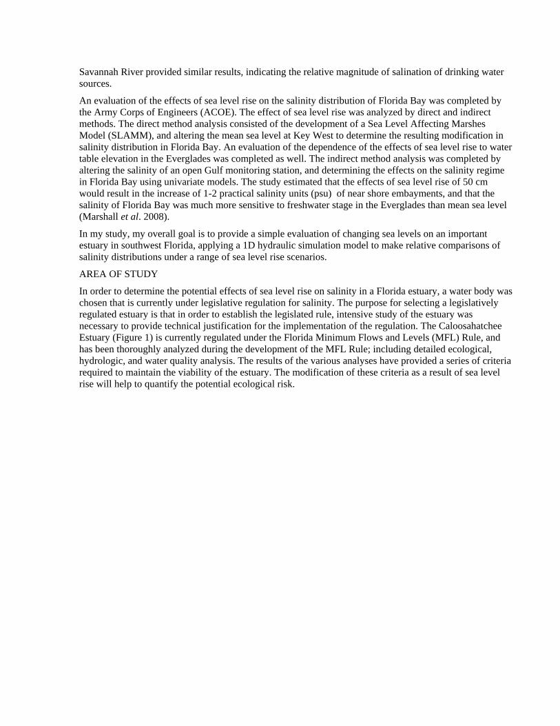
An evaluation of the effects of sea level rise on the salinity distribution of Florida Bay was completed by

the Army Corps of Engineers (ACOE). The effect of sea level rise was analyzed by direct and indirect

methods. The direct method analysis consisted of the development of a Sea Level Affecting Marshes

Model (SLAMM), and altering the mean sea level at Key West to determine the resulting modification in

salinity distribution in Florida Bay. An evaluation of the dependence of the effects of sea level rise to water

table elevation in the Everglades was completed as well. The indirect method analysis was completed by

altering the salinity of an open Gulf monitoring station, and determining the effects on the salinity regime

in Florida Bay using univariate models. The study estimated that the effects of sea level rise of 50 cm

would result in the increase of 1-2 practical salinity units (psu) of near shore embayments, and that the

salinity of Florida Bay was much more sensitive to freshwater stage in the Everglades than mean sea level

(Marshall et al. 2008).

In my study, my overall goal is to provide a simple evaluation of changing sea levels on an important

estuary in southwest Florida, applying a 1D hydraulic simulation model to make relative comparisons of

salinity distributions under a range of sea level rise scenarios.

AREA OF STUDY

In order to determine the potential effects of sea level rise on salinity in a Florida estuary, a water body was

chosen that is currently under legislative regulation for salinity. The purpose for selecting a legislatively

regulated estuary is that in order to establish the legislated rule, intensive study of the estuary was

necessary to provide technical justification for the implementation of the regulation. The Caloosahatchee

Estuary (Figure 1) is currently regulated under the Florida Minimum Flows and Levels (MFL) Rule, and

has been thoroughly analyzed during the development of the MFL Rule; including detailed ecological,

hydrologic, and water quality analysis. The results of the various analyses have provided a series of criteria

required to maintain the viability of the estuary. The modification of these criteria as a result of sea level

rise will help to quantify the potential ecological risk.

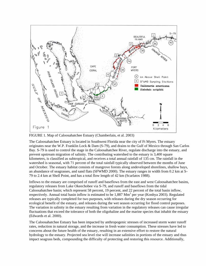
FIGURE 1. Map of Caloosahatchee Estuary (Chamberlain, et al. 2003)

The Caloosahatchee Estuary is located in Southwest Florida near the city of Ft Myers. The estuary

originates near the W.P. Franklin Lock & Dam (S-79), and drains to the Gulf of Mexico through San Carlos

Bay. S-79 is used to control the stage in the Caloosahatchee River, regulate discharge into the estuary, and

prevent upstream migration of salinity. The contributing watershed to the estuary is 3,400 square

kilometers, is classified as subtropical, and receives a total annual rainfall of 135 cm. The rainfall in the

watershed is seasonal, with 71 percent of the total rainfall typically observed between the months of June

and October. The estuary habitat consists of mangrove forests along undeveloped shorelines, shallow bays,

an abundance of seagrasses, and sand flats (SFWMD 2000). The estuary ranges in width from 0.2 km at S-

79 to 2.4 km at Shell Point, and has a total flow length of 42 km (Scarlatos 1988).

Inflows to the estuary are comprised of runoff and baseflows from the east and west Caloosahatchee basins,

regulatory releases from Lake Okeechobee via S-79, and runoff and baseflows from the tidal

Caloosahatchee basin; which represent 58 percent, 19 percent, and 22 percent of the total basin inflow,

respectively. Annual total basin inflow is estimated to be 1,887 Mm3 per year (Konhya 2003). Regulated

releases are typically completed for two purposes, with releases during the dry season occurring for

ecological benefit of the estuary, and releases during the wet season occurring for flood control purposes.

The variation in salinity in the estuary resulting from variation in the regulatory releases can cause irregular

fluctuations that exceed the tolerance of both the oligohaline and the marine species that inhabit the estuary

(Edwards et al. 2000).

The Caloosahatchee Estuary has been impacted by anthropogenic stresses of increased storm water runoff

rates, reduction in natural storage, and the increase in fresh water consumption. These stresses have led to

concerns about the future health of the estuary, resulting in an extensive effort to restore the natural

hydrology to the estuary. Projected sea level rise will increase salinities in portions of the estuary and thus

impact seagrass beds, compounding the difficulty of protecting and restoring this resource. Additionally,

the estuary is unable to adjust to the effects of sea level rise due to the salinity partition imposed by S-79,

where oligohaline species would otherwise be able to migrate upstream in the occurrence of increased

salinities in currently occupied habitats. Importantly, the effects of sea level rise have yet to be quantified

for the estuary, and could have a significant impact on the management plan for the estuary, especially the

legally required MFL.

FLOW REGULATION RULES AND SALINITY

Florida water management agencies are required to develop rules which describe the minimum allowable

quantity of managed freshwater flows that are necessary to maintain the ecology of targeted water bodies in

the state. The determination of such Minimum Flows and Levels (MFL) needed for the ecology of the

Caloosahatchee Estuary is a highly contested issue between various stakeholders.

Water Management Districts are the primary agencies responsible for the development of the MFL Rules

for all priority water bodies in Florida. The establishment of MFL Rules is required under subsection

373.042(2) of the Florida Statutes (F.S.). MFL Rules are designed to prevent any significant harm to

Florida water bodies by determining the minimum flow necessary to allow for habitat preservation,

beneficial use, and allocated consumptive use. Minimum levels are developed for lakes, wetlands, and

aquifers, and minimum flows are developed for rivers, streams, and estuaries. Once MFL Rules have been

implemented they are commonly used to evaluate whether any further consumptive use from a water body

is permissible, and to help develop operation protocols for water control structures (SFWMD 2011).

In accordance with Florida law, Districts must use the best available information and methods to develop

MFL Rules. Therefore, extensive evaluations are necessary to determine the extent and frequency that

flows and levels can be reduced without causing significant harm, where significant harm is defined as the

loss of water resource function that will take more than two years to recover. Due to the complex

interactions that occur within natural water bodies, it is commonplace for models to be implemented when

developing technical justifications for MFLs. Depending on the complexity of the hydrologic interactions

occurring within a water body, statistical and simulation models for hydrology, hydraulics, water quality,

and ecology may be required (SFWMD 2003).

In September 2000 the South Florida Management District first proposed the MFL Rule for the

Caloosahatchee. The September 2000 report identified the 640 acre bed of seagrass species Vallisneria

americana, commonly known as wild celery, as the primary resource within the Caloosahatchee that would

be affected from reduced freshwater flows. The wild celery habitat in the Caloosahatchee estuary is located

in the low salinity zone between Ft Myers and S-79. Wild celery is a seagrass that is adapted to low salinity

zones of an estuary, and therefore increases in salinity in the upper portion of the Caloosahatchee Estuary

would result in losses of that habitat (Edwards et al. 2000).

Using the best information known on the salinity requirements of wild celery, SFWMD (2003) used a

simple regression model of flow at S-79 vs. salinity within the wild celery habitat to estimate the freshwater

inflow required at S-79 to maintain appropriate salinities for that habitat.

The MFL Rule for the Caloosahatchee was adopted in September 2001, after an independent panel of

reviewers (Edwards et al. 2000) concluded that the scientific basis for the Rule was the best information

available at the time.

The 2001 MFL rule states that:

“A minimum mean monthly flow of 300 cfs (8.5 m3/s) is necessary to maintain sufficient salinities

at S-79 in order to prevent a MFL exceedance. A MFL exceedance occurs during a 365 day period,

when:

(a) A 30-day average salinity concentration exceeds 10 parts per thousand at the Ft.

Myers salinity station (measured at 20% of the total river depth from the water surface […]; or

(b) A single, daily average salinity exceeds a concentration of 20 parts per thousand

at the Ft. Myers salinity station.

Exceedance of either paragraph (a) or (b), for two consecutive years is a violation of the MFL.”

The initial study that was completed to determine the MFL for the estuary predicted that the MFL criteria

would be frequently exceeded (i.e., significant harm to the wild celery community would occur) under

2000 operation protocols for controlled releases to the estuary from Lake Okeechobee. Therefore, the MFL

study and the MFL Rule included a science-based strategy for prevention and recovery for the MFL

exceedances. The prevention and recovery strategy included additional storage in the freshwater portion of

the basin to be used during low flow conditions, revised operational protocols, revised consumptive use

permitting procedures, and required continual refinement of the MFL if and when needed (Edwards et al

2000).

A peer review of the MFL study completed in 2000 by the USGS and various academic institutions

identified four major areas of concern (SFWMD 2003); they are, lack of a hydrodynamic/salinity model,

lack of a numerical population model for Vallisneria americana, no quantification of the habitat value of

Vallisneria beds, and lack of documentation of the effects of MFL flows on downstream estuarine biota

(SFWMD 2003).

This led to research efforts to further support the MFL criteria and refine the "prevention and recovery"

strategy for the Caloosahatchee Estuary (SFWMD 2003). A variety of research efforts were utilized.

Monitoring data were used to evaluate the effects of the salinity variations on fish larvae, plankton, and

oysters; field monitoring and mesocosm experiments were performed to determine the maximum allowable

salinity concentrations within the estuary that is protective of the current ecosystem (Doering 2003); a

hydrodynamic model was applied to determine the salinity distribution in the estuary for various flow

conditions (Qiu 2003); and a basin model was developed to determine the expected freshwater flow

contribution to the estuary from the tidal portion of the basin (Konyha 2003).

Field monitoring and mesocosm experiments were performed to evaluate the sensitivity of wild celery to

increased concentrations of salinity, as part of the MFL Rule technical justification (Doering 2003).

Doering (2003) determined that wild celery growth decreased as salinity increased, and that mortality rates

increased when salinity concentrations exceeded 15 ppt. It was determined that salinities greater than 18

ppt would cause a 50 percent mortality within 38 days, and a salinity of 20 ppt would cause a 50 percent

mortality within 16 days. The field monitoring and experiments demonstrated that wild celery can

withstand salinities less than 10 ppt for greater than a month and salinities less than 20 ppt for 3 days.

Therefore, salinities of 10 ppt and 20 ppt were chosen to regulate long term and acute exposures,

respectively (SFWMD 2003).

As part of this overall research effort (SFWMD 2003), a hydrodynamic model (Sheng 2001) was applied to

the estuary to determine the salinity distribution under various freshwater flow conditions within the

estuary (Qiu 2003). CH3D is a 3-dimensional finite difference hydrodynamic model that employs a

curvilinear grid developed to evaluate surface elevation, 3-D velocity, salinity, and density (Sheng 1987,

1989, 2001). The CH3D model for the Caloosahatchee estuary is comprised of 145 by 225 horizontal grid

cells with 8 vertical layers. Inputs to the model included freshwater inflow, tides, wind, rainfall, and

evapotranspiration. The model was calibrated with 77 days of observations (October 15, 2000 to December

31, 2000). The calibrated model was then applied in six scenarios of varying S-79 inflows, assuming no

other inputs (such as rainfall or groundwater contribution) and conducting model simulations of 40 days to

achieve equilibrium conditions. The salinity concentrations at four locations along the river/estuary were

averaged over the last 10 days of simulation, providing the flow-salinity response curves shown in Figure 2

(Qiu 2003). Qiu (2003) determined that a total flow of 14.2 m3/s of total freshwater inflow to the system

was required to maintain the appropriate salinity distribution in the upper estuary that is protective of wild

celery communities in the Ft. Meyers location.

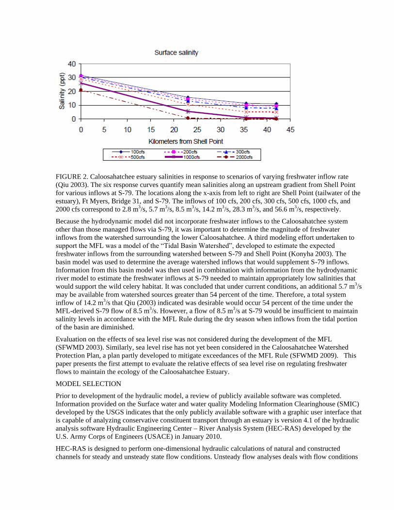
FIGURE 2. Caloosahatchee estuary salinities in response to scenarios of varying freshwater inflow rate

(Qiu 2003). The six response curves quantify mean salinities along an upstream gradient from Shell Point

for various inflows at S-79. The locations along the x-axis from left to right are Shell Point (tailwater of the

estuary), Ft Myers, Bridge 31, and S-79. The inflows of 100 cfs, 200 cfs, 300 cfs, 500 cfs, 1000 cfs, and

2000 cfs correspond to 2.8 m3/s, 5.7 m3/s, 8.5 m3/s, 14.2 m3/s, 28.3 m3/s, and 56.6 m3/s, respectively.

Because the hydrodynamic model did not incorporate freshwater inflows to the Caloosahatchee system

other than those managed flows via S-79, it was important to determine the magnitude of freshwater

inflows from the watershed surrounding the lower Caloosahatchee. A third modeling effort undertaken to

support the MFL was a model of the “Tidal Basin Watershed”, developed to estimate the expected

freshwater inflows from the surrounding watershed between S-79 and Shell Point (Konyha 2003). The

basin model was used to determine the average watershed inflows that would supplement S-79 inflows.

Information from this basin model was then used in combination with information from the hydrodynamic

river model to estimate the freshwater inflows at S-79 needed to maintain appropriately low salinities that

would support the wild celery habitat. It was concluded that under current conditions, an additional 5.7 m3/s

may be available from watershed sources greater than 54 percent of the time. Therefore, a total system

inflow of 14.2 m3/s that Qiu (2003) indicated was desirable would occur 54 percent of the time under the

MFL-derived S-79 flow of 8.5 m3/s. However, a flow of 8.5 m3/s at S-79 would be insufficient to maintain

salinity levels in accordance with the MFL Rule during the dry season when inflows from the tidal portion

of the basin are diminished.

Evaluation on the effects of sea level rise was not considered during the development of the MFL

(SFWMD 2003). Similarly, sea level rise has not yet been considered in the Caloosahatchee Watershed

Protection Plan, a plan partly developed to mitigate exceedances of the MFL Rule (SFWMD 2009). This

paper presents the first attempt to evaluate the relative effects of sea level rise on regulating freshwater

flows to maintain the ecology of the Caloosahatchee Estuary.

MODEL SELECTION

Prior to development of the hydraulic model, a review of publicly available software was completed.

Information provided on the Surface water and water quality Modeling Information Clearinghouse (SMIC)

developed by the USGS indicates that the only publicly available software with a graphic user interface that

is capable of analyzing conservative constituent transport through an estuary is version 4.1 of the hydraulic

analysis software Hydraulic Engineering Center – River Analysis System (HEC-RAS) developed by the

U.S. Army Corps of Engineers (USACE) in January 2010.

HEC-RAS is designed to perform one-dimensional hydraulic calculations of natural and constructed

channels for steady and unsteady state flow conditions. Unsteady flow analyses deals with flow conditions

that vary temporally and spatially. The hydraulic software is capable of analyzing the addition of culverts,

bridges, levees, tributaries, storage areas and traversing dams in the flow network. In addition to the flow

routing capability, HEC-RAS incorporates numerous auxiliary components such as dam breach analysis,

sediment transport, river encroachment analysis, and water quality modeling. The hydraulic calculations

performed in HEC-RAS are completed using one dimensional energy equations, and the unsteady flow

equation solver was adapted from Dr. Robert L. Barkau's UNET model. Version 4.1 of HEC-RAS allows

for water quality analysis of negative flows that are observed within an estuary during an incoming tide, a

feature that was not included in version 4.0 (USACE 2010).

The USACE has also developed an extension of ArcGIS that is capable of performing spatial analysis of

Digital Elevation Models (DEMs), and extracting geometric information from the DEM for direct import

into HEC-RAS. HEC-GeoRAS is also capabable of importing HEC-RAS results into ArcGIS, and

automatically generating inundation boundaries for a river system (USACE 2010).

In contrast to the complex CH3D model developed for the MFL Rule justification, HEC-RAS is a one-

dimensional hydraulic model that does not account for multi-directional flow paths or variations in fluid

density. However, given the long, slender geometry of the estuary, a one-dimensional hydraulic model was

expected to reasonably represent the estuarine dynamics since there are few bays and large tributaries

within the area of study (SFWMD 2000).

MODEL IMPLEMENTATION - HYDRAULICS

The model domain was selected to extend from S-79 through San Carlos Bay (Figure 1) and 17 km into the

Gulf of Mexico. The decision to the extend the model into the Gulf of Mexico was made to reduce the

effects of boundary conditions, and the reliance on observed data to describe the conditions at the model

boundary. This is based on the observation that the salinity distribution plots developed by the CH3D

model (see Figure 2) demonstrate that the salinity at Shell Point is dependent on the total inflow to the

Caloosahatchee estuary, and cannot be assumed to be a constant value of 35 ppt; which is an average value

for the Gulf of Mexico.

In order to capture the bathymetry of the Caloosahatchee estuary for the HEC-RAS model, HEC-GeoRAS

was utilized. The 2005 bathymetry dataset for Southwest Florida (that was obtained by the USGS working

in conjunction with the SFWMD) was utilized to capture the 1D channel geometry from the Gulf of

Mexico to 33 km above Shell Point (SFWMD 2005a). The channel geometry for the portion of the estuary

33 km above Shell Point to S-79 was digitized from the cross sections presented in SFWMD Technical

Report 88 (TR-88) [(Scarlatos 1988)]. The overbank portions of all cross sections were described to an

elevation of 1.5 m NAVD 88 using the Southwest Florida topographic dataset (SFWMD 2005b). The

spatial resolution of the bathymetric dataset is 90 m, and the spatial resolution of the topographic dataset is

30 m. The two GIS datasets were clipped for the area of interest and merged into a continuous Triangular

Irregular Network (TIN). The alignment of the channel centerline of the estuary between S-79 and Shell

Point was obtained from the National Hydrography Dataset (NHD) for subbasin 03090205 published by the

USGS. The layout of the cross sections was chosen to describe non-linear changes in channel width or

depth, and the location of the cross sections 33 Km above Shell Point were digitized according to TR-88.

The cross section data that was obtained from TR-88 was converted into geo-referenced points, and used to

modify the TIN to describe upper estuary channel geometry. Additionally, an assumed crest elevation of

1.5 m NAVD 88 was incorporated into the TIN to represent S-79, and captured in HEC-GeoRAS as an

inline structure layer. The channel geometry and stream alignment were generated into an import file for

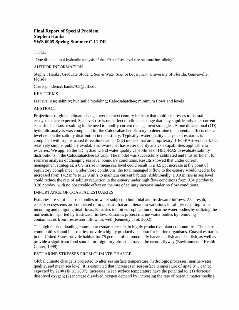
HEC-RAS directly through HEC-GeoRAS. The layout of the channel cross sections and stream centerline

is depicted in Figure 3.

FIGURE 3. Layout of HEC-GeoRAS layers. Sources: Base Map (ESRI Library – US street map layer), Centerline (NHD

dataset for subbasin 03090205 with modifications), Cross Sections (Scarlatos 1988 with modification), Monitoring Stations

(SFWMD – Salinity Monitoring Stations).

Following the import of the geometry file, a calibration of the Manning's n values for the hydraulic model

was completed to replicate observed tidal data. In order to facilitate the calibration of Manning's n values,

observed tidal data at SFWMD monitoring station MARKH located near Shell Point was incorporated as

the tailwater boundary condition, rather than trying to extrapolate the tidal stages in the Gulf of Mexico;

since a monitoring station further downstream of Shell Point is not available. The headwater boundary

condition was the observed discharge at SFWMD monitoring station S-79 T (located at the tailwater of S-

79) with additional inflow that was assumed to be representative of the groundwater inflow between S-79

and SFWMD salinity monitoring station FTMYERS. In subsequent salinity simulations it was determined

that the representation of groundwater inflow as lateral inflow into the estuary with 0 ppt salinity caused

instability in the water quality simulation module. Therefore all freshwater inflow into the estuary had to be

input in the headwater at S-79. The total inflow at S-79 was chosen to be representative of the total inflow

at Ft Myers since salinity monitoring station FTMYERS is the regulatory point of compliance for the MFL

Rule. The total groundwater inflow into the estuary was approximated as 22 percent of the 30 day average

discharge at S-79 in accordance with the estimate by Konyha (2003) that the groundwater inflow to the

estuary comprised 22 percent of the total inflow with the remainder entering the estuary at S-79. The

groundwater inflow between S-79 and Ft Myers was estimated to be a fraction of the total groundwater

inflow to the estuary based on the fractions provided by Konhya (2003) who estimated that 64.4 percent of

the groundwater inflow to the estuary occurred between S-79 and Ft Myers.

The observed stage at NOAA monitoring station 8725520 located near Ft Myers and SFWMD monitoring

station VAL-I75 located near the I75 overpass were input into HEC-RAS to facilitate comparison to the

observed stages in the estuary. The model was simulated from November 1, 2007 to November 27, 2007.

Following the initial simulation and adjustment of the Manning's n value in the estuary, it was observed

that the mean sea level calculated during the simulation for both Ft Myers and VAL-I75 were greater than

the observed mean sea level for the simulation period by approximately 15 cm, but that the calculated

ranges at both locations closely replicated the observed ranges. Additionally, it was noted that the observed

mean sea level at Shell Point was 3 cm NAVD 88, and -10 cm NAVD 88 at Ft Myers and VAL-I75.

Therefore, the tidal data at the tailwater boundary condition was reduced by 14.9 cm, and the simulation

was rerun. The comparison of observed and calculated values for Ft Myers and VAL-I75 are presented

below.

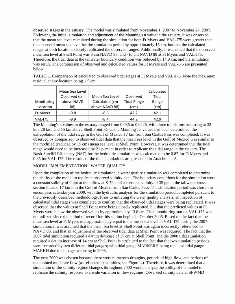
TABLE 1. Comparison of calculated to observed tidal stages at Ft Myers and VAL-I75. Note the maximum

residual at any location being 1.5 cm.

Monitoring Location

Mean Sea Level Observed (cm above NAVD

88)

Mean Sea Level Calculated (cm

above NAVD 88)

Observed Tidal Range

(cm)

Calculated Tidal

Range (cm)

Ft Myers -9.8 -8.6 42.2 42.1

VAL-I75 -9.9 -8.4 44.2 42.9

The Manning's n values in the estuary ranged from 0.036 to 0.0225, with three transitions occurring at 33

km, 28 km, and 15 km above Shell Point. Once the Manning's n values had been determined, the

extrapolation of the tidal stage in the Gulf of Mexico 17 km from San Carlos Pass was completed. It was

observed by comparison to observed tidal data that the mean sea level in the Gulf of Mexico was similar to

the modified (reduced by 15 cm) mean sea level at Shell Point. However, it was determined that the tidal

range would need to be increased by 21 percent in order to replicate the tidal range in the estuary. The

Nash-Sutcliff Efficiency (NSE) for the hydraulic simulation was calculated to be 0.87 for Ft Myers and

0.85 for VAL-I75. The results of the tidal simulations are presented in Attachment A.

MODEL IMPLEMENTATION - WATER QUALITY

Upon the completion of the hydraulic simulation, a water quality simulation was completed to determine

the ability of the model to replicate observed salinity data. The boundary conditions for the simulation were

a constant salinity of 0 ppt at the inflow at S-79, and a constant salinity of 35 ppt at the tailwater cross

section located 17 km into the Gulf of Mexico from San Carlos Pass. The simulation period was chosen to

encompass calendar year 2000, with the hydraulic analysis for the simulation period completed pursuant to

the previously described methodology. Prior to initiating the water quality analysis, an inspection of

calculated tidal stages was completed to confirm that the observed tidal stages were being replicated. It was

observed that the values at Shell Point were being closely replicated, but that the predicted values at Ft

Myers were below the observed values by approximately 13.8 cm. Tidal monitoring station VAL-I75 was

not utilized since the period of record for this station begins in October 2006. Based on the fact that the

mean sea level at Ft Myers was approximately equal to the mean sea level at VAL-I75 during the 2007

simulation, it was assumed that the mean sea level at Shell Point was again incorrectly referenced to

NAVD 88, and that an adjustment of the observed tidal data at Shell Point was required. The fact that the

2007 tidal simulation required a datum decrease of 15 cm at Shell Point, and the 2000 tidal simulation

required a datum increase of 14 cm at Shell Point is attributed to the fact that the two simulation periods

were recorded by two different tidal gauges; with tidal gauge MARKERH being replaced tidal gauge

MARKH due to damage occurring in 2003.

The year 2000 was chosen because there were numerous droughts, periods of high flow, and periods of

maintained moderate flow (as reflected in salinities, see Figure 4). Therefore, it was determined that a

simulation of the salinity regime changes throughout 2000 would analyze the ability of the model to

replicate the salinity response to a wide variation in flow regimes. Observed salinity data at SFWMD

monitoring stations SANIBEL, SHELL POINT, FT MYERS, BRIDGE 31, and S-79 was collected and

incorporated into to the model to facilitate comparison and calibration. The data provided by the SFWMD

is comprised of specific conductance and temperature for both the surface and bottom interval at each

location. Since the MFL Rule is dependent on surface salinity, daily surface readings were utilized. The

specific conductance and temperature readings were converted into salinity values referenced to the

Practical Salinity Scale of 1978 (PSS 78) using the methodology and constants provided in the 19th edition

of standard methods (Clesceri et al. 1996). The initial salinity distribution in the estuary was set to equal

the observed values for January 1, 2000. The dispersion coefficients in the estuary were computed in HEC-

RAS for each water quality cell in accordance with Fischer’s equation (USACE 2010).

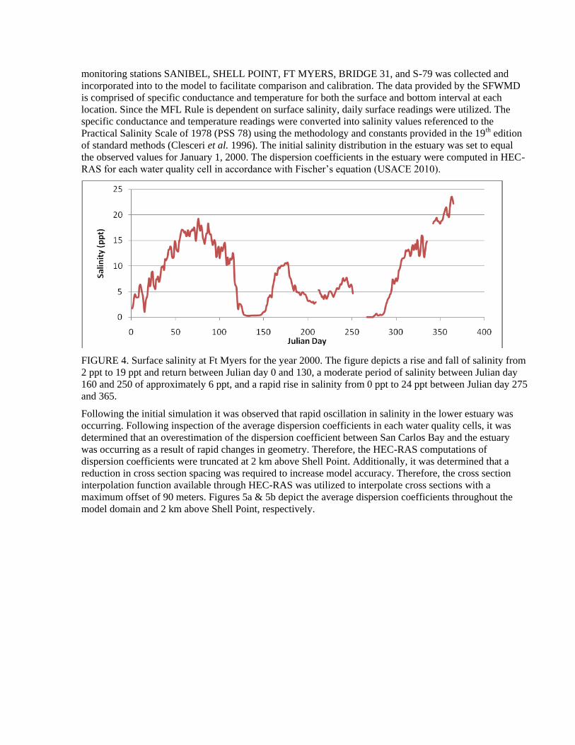
FIGURE 4. Surface salinity at Ft Myers for the year 2000. The figure depicts a rise and fall of salinity from

2 ppt to 19 ppt and return between Julian day 0 and 130, a moderate period of salinity between Julian day

160 and 250 of approximately 6 ppt, and a rapid rise in salinity from 0 ppt to 24 ppt between Julian day 275

and 365.

Following the initial simulation it was observed that rapid oscillation in salinity in the lower estuary was

occurring. Following inspection of the average dispersion coefficients in each water quality cells, it was

determined that an overestimation of the dispersion coefficient between San Carlos Bay and the estuary

was occurring as a result of rapid changes in geometry. Therefore, the HEC-RAS computations of

dispersion coefficients were truncated at 2 km above Shell Point. Additionally, it was determined that a

reduction in cross section spacing was required to increase model accuracy. Therefore, the cross section

interpolation function available through HEC-RAS was utilized to interpolate cross sections with a

maximum offset of 90 meters. Figures 5a & 5b depict the average dispersion coefficients throughout the

model domain and 2 km above Shell Point, respectively.

FIGURE 5a. Average dispersion coefficients

throughout the model domain. The figure

depicts a six fold increase below Shell Point.

FIGURE 5b. Average dispersion coefficients 2 km

above Shell Point. The figure depicts a uniform

decrease in values.

The NSE for the calculated salinity values for year 2000 were determined to be 0.23, 0.42, 0.67, 0.64, and

0.61 for salinity monitoring stations SANIBEL, SHELL POINT, FT MYERS, BRIDGE 31, and S-79, respectively.

The low NSE for Sanibel and Shell Point are attributed to the constant salinity of 35 psu at the tailwater boundary

conditions. This is especially true when the conditions in San Carlos Bay are hypersaline. An evaluation of the NSE

when the observed salinity values at Sanibel are below 35 psu, estimates values of 0.32 and 0.46 at Sanibel and Shell

Point, respectively. However the effect of this boundary condition does not cause an undesirable NSE at Ft Myers.

The greatest disparity between observed and calculated values at Ft Myers was observed to occur during

the wet season. Therefore, it is assumed that of the 22 percent of the total estuary inflow from groundwater,

that a recognizably more substantial fraction is incurred to the estuary during the wet season. The results of

the salinity simulation are presented in Attachment B.

MODEL APPLICATION - ASSUMPTIONS

The potential effects of sea level rise on the salinity distribution in the estuary was evaluated for

three separate scenario combinations of sea level rise and managed inflows. Incremental increases

in mean sea level of 0.3 m were analyzed for all scenarios up to a total increase of 0.9 m. The first

scenario was developed to evaluate the effects of incremental increases in mean sea level under a

constant inflow of 14.2 m3/s at S-79, which represents the recommended total inflow to the estuary

to maintain the current habitat viability. The second scenario was to evaluate the change in the rate

of salinity increase under no flow conditions. The evaluation was completed with initial salinity

values set to represent moderate conditions, and subsequent inflow conditions at S-79 equal to 0.

The third scenario was developed to evaluate the change in the rate of salinity decrease under high

flow conditions. The initial salinity values were set to represent acute conditions where the salinity

at Ft Myers was 20 ppt, and the inflow conditions at S-79 were a constant value of 36.8 m3/s. For

all scenarios the values presented by the CH3D modeling effort were utilized for comparative

purposes (Qiu 2003). The tidal boundary condition for all scenarios is a synthetic stage hydrograph

developed from the stage datums for Shell Point. The synthetic stage hydrograph was developed by

calculating the Mean Higher High Water (MHHW), Mean High Water (MHW), Mean Low Water

(MLW), Mean Lower Low Water (MLLW), and Mean Sea Level (MSL) datums for Shell Point for

all available stage recordings from monitoring station MARKERH (January 22, 1992 00:15 to July

19, 2001 0:00); then increasing each datum by 13.8 cm and multiplying by 1.21 (as described in the

implementation of the hydraulics simulation above). The sinusoidal hydrograph centered around

the extrapolated MSL datum was generated by assuming that each datum was equally distributed

across the diurnal period, and the incremental increases in mean sea level were assumed to not

affect the tidal ranges. The synthetic stage hydrograph developed from current tidal datums is

illustrated in Figure 6. The results of the three scenarios are presented in Attachment C.

FIGURE 6. Synthetic tidal hydrograph developed from current tidal datums. Values of MHHW,

MHW, MLW, MLLW, and MSL extrapolated to 21 km below Shell Point were determined to be

5.4 cm NAVD 88, -5.7 cm NAVD 88, -45.1 cm NAVD 88, -53.8 cm NAVD 88, and -21.9 cm

NAVD 88, respectively.

MODEL APPLICATION - RESULTS

The evaluations of the three scenario combinations demonstrated that salinity changes within the estuary

could be observed under significant increases in sea level, if alterations in current management strategies

do not occur. Scenario 1 indicated that a 0.9 m rise in mean sea level will increase the average salinity at Ft

Myers (ca. 23 km from Shell Point) from 15.6 ppt to 20.1 ppt if the total basin inflow is 14.2 m3s (Figure

C1). The highest sea level rise led to salinity at Ft Myers that was 29 percent higher than without sea level

rise (Figure 7). With linear increases (0.3 - 0.9 m) in mean sea level rise for scenario one, there was an

approximately linear increase in salinity. The percent increase was less at Shell Point (9 percent) and

greater at Bridge 31 and S-79 (150 percent and 340 percent, respectively.

FIGURE 7. Response of surface salinity at Ft Myers to increases in mean sea level, with total inflows of

14.2 m3/s at S-79..

An iteration of flows at S-79 for scenario 1 demonstrated that an increase in total S-79 inflow to 22.9 m3/s

would be required to maintain the salinity distribution initially calculated for the current mean sea level.

The subsequent additional volume of flow to maintain an average flow of 22.9 m3/s versus an average flow

of 14.2 m3/s is estimated to be 275 Mm3/year. The second scenario demonstrated that no observable change

in the relative rates of salinity increase under no flow conditions will occur as a result of sea level rise (all

increase at similar rates, Figure C2). However, the third scenario demonstrated that a reduction (in the rate

of salinity decrease) from 0.50 ppt/day to 0.28 ppt/day may occur under high flow conditions (36.8 m3/s

total inflow) under a 0.9 m increase in mean sea level (rates of salinity decreases vary among scenarios,

Figure C3). As observed in previous scenarios, the incremental increases in mean sea level resulted in a

linear change in salinity regime in the estuary.

MODEL UNCERTAINTIES AND LIMITATIONS

The HEC-RAS simulation resulting in a salinity of 15.6 ppt at Ft Myers with an inflow of 14.2 m3/s and no

sea level rise is greater than the CH3D predicted value of 10.6 ppt (Figure 8). The disparity is possibly due

to an apparent under prediction by the CH3D model when compared to observed values (SFWMD 2003),

and an apparent over prediction by HEC-RAS when compared to observed values, with the expected value

being located between the two estimations (Qiu 2003).

FIGURE 8. Comparison of predicted salinity distribution in the estuary between HEC-RAS and CH3D for

total inflow of 14.2 m3/s at S-79.

The HEC-RAS model tended to overestimate salinities (compared to observations) during the wet season at

Ft Myers, likely due to the omission of runoff contributions from the watershed. Similar to previous

modeling efforts (SFWMD 2003), a number of assumptions were made to accommodate such uncertainties,

and improved modeling and data may improved our understanding of those contributions to total

Caloosahatchee flows. Further study to possibly develop a hydrologic model that could interface with the

HEC-RAS model, such as through HEC-HMS, would likely be fruitless; since this study demonstrates that

inflows of 0 ppt salinity into the estuary other than at the headwater causes HEC-RAS instability. However,

further troubleshooting could be completed to determine if the water quality module could allow freshwater

inflow into the estuary if the inflow points were represented as tributaries, and water control structures were

implemented as necessary. Contrary to this effort is the observed instability resulting from the

representation of San Carlos Bay and Pine Island Sound as tributaries that merged with the model near

Sanibel.

The model simulations at SFWMD salinity monitoring stations BRIDGE 31 and S79 under predicted

surface salinity compared to observed data. It is proposed that these results are inaccurate due to the rapid

channel geometry change that occurs 33 Km above Shell Point, but that the inaccuracy at these locations do

not significantly affect the accuracy further downstream at Ft Myers.

The estimates of salinity increase of 4.5 ppt at Ft Myers resulting from a 0.9 m rise in mean sea level may

appear to be insignificant given the limited model sensitivity, and the relatively minimal predicted increase;

especially since the HEC-RAS estimate is greater than the CH3D estimate for surface salinity at Ft Myers

under a constant flow of 14.2 m3/s by 5 ppt. However, it is proposed that the expected increase of 4.5 ppt,

and the subsequently required flow increase of 8.7 m3/s to restore the initial salinity distribution is a reliable

estimate based on the ability of the model to represent the modification of the salinity regime in the estuary

as a result of changes in the flow conditions. The implications of the potential flow increase that would be

required become especially significant when put into the context of the reservoir storage required to deliver

such additional flow.

The analysis of estuarine water quality utilizing HEC-RAS can also be limited by various geometric

aspects. The necessity to include multiple tributaries into the estuary may cause instabilities in the water

quality module. Also rapid variations in the Fischer dispersion coefficient can cause inconsistent estimates,

and the inclusion of multiple water quality structures such as levees and storage areas may possibly cause

computational instabilities. As previously mentioned, if lateral inflow boundary conditions are incorporated

in the simulation, then a significant disparity in inflow concentrations and in-situ concentrations cannot be

present; otherwise computational instabilities may occur.

CONCLUSIONS

This study demonstrates that a one-dimensional hydraulic analysis of estuaries can provide informative

estimates of the water quality responses to scenarios of sea level rises and counter-acting freshwater inputs.

The agreement between simulated and observed data was sufficient to indicate that the general response of

the salinity distribution in the estuary to flow conditions is reasonably represented. Applications of this

model provided the first estimates of the sensitivity of salinity distributions to changes in long-term sea

level, and associated assumptions of the upstream freshwater flows that may be necessary to maintain

healthy seagrass beds in the Caloosahatchee Estuary

We recognize the limitations of this model and it simplifying assumptions (in the above section).

Nevertheless, this model excercise provided a broad understanding to the relative magnitudes of managed

flows that may be necessary to maintain existing salinity distributions in the Caloosahatchee Estuary under

different scenarios of sea level rise. While the magnitudes of the salinity changes may be relatively small

(ca. 5 ppt) among scenarios, other studies may use these results to estimate whether the potential changes

are ecologically significant over long time scales. One of the most significant aspects of this study is its

relative ease (i.e., low cost) of implementation, providing bounding information that can spur further

consideration of sea level rise on MFL refinement for the Caloosahatchee Estuary.

REFERENCES

Chamberlain, R.H., Doering, P.H., Haunert, K.M., & Crean, D. South Florida Water Management

District, (2003). Technical documentation to support development of minimum flows and levels

for the caloosahatchee river and estuary: appendix c impacts of freshwater inflows on the

distribution of zooplankton and ichthyoplankton in the caloosahatchee estuary, florida

Retrieved from

http://www.sfwmd.gov/portal/page/portal/xrepository/sfwmd_repository_pdf/mfl_caloos2003a

pp.pdf

Clesceri, L. S., Eaton, A. D., Greenberg, A. E., Franson, M. A. H., American Public Health

Association., American Water Works Association., & Water Environment Federation. (1996).

Standard methods for the examination of water and wastewater: 19th edition supplement.

Washington, DC: American Public Health Association.

Conrad, P., Roehl, E., Sexton, C., Tufford, D., Carbone, G., Dow, K., Cook, J., (2010a) Estimating

salinity intrusion effects due to climate change along the grand strand of the south carolina

coast Retrieved from

http://acwi.gov/sos/pubs/2ndJFIC/Contents/7E_Conrads_12_20_09_final.pdf

Conrad, P., Roehl, E., Sexton, C., Tufford, D., Carbone, G., Dow, K., Cook, J., (2010b) Estimating

salinity intrusion effects due to climate change on the Lower Savannah River Estuary

Retrieved from http://www.cisa.sc.edu/images/SCEC2010_Sav_CC.pdf

Doering, P.H., South Florida Water Management District, (2003). Technical documentation to

support development of minimum flows and levels for the caloosahatchee river and estuary:

appendix d salinity tolerance of vallisneria and salinity criteria Retrieved from

http://www.sfwmd.gov/portal/page/portal/xrepository/sfwmd_repository_pdf/mfl_caloos2003a

pp.pdf

Environmental Health Center. 1998. Coastal Challenges: A Guide to Coastal and Marine Issues.

National Safety Council, Washington, DC.

Edwards, R.E., Lung, W., Montagna, P.A., & Windom, H.L. South Florida Water Management

District, (2000). Final Review Report: Caloosahatchee minimum flow Retrieved from

http://www.sfwmd.gov/portal/page/portal/xrepository/sfwmd_repository_pdf/mfl_caloos_peerr

ev_112000.pdf

Environmental Protection Agency, (2010). Coastal zones and sea level rise Retrieved from

http://www.epa.gov/climatechange/effects/coastal/index.html

Hull, C.H.J. and J.G.Titus (eds), (1986). Greenhouse Effect, Sea Level Rise, and Salinity in the

Delaware Estuary.. Washington, D.C.: U.S. Environmental Protection Agency and Delaware

River Basin Commission.

Intergovernmental Panel on Climate Change, (2007). Climate change 2007: contribution of

working group ii to the fourth assessment report of the intergovernmental panel on climate

change Retrieved from http://www.ipcc-wg2.org/index.html

Natioal Oceanic and Atmospheric Administration, (2008). Mean sea level trend - 8725520 fort myers,

florida Retrieved from http://tidesandcurrents.noaa.gov/sltrends/sltrends_station.shtml?stnid=8725520

Kennedy, V., Twilley, R., Kleypas, J., Cowan Jr., J., & Hare, S., (2002) Environment: coastal and marine

ecosystems & global climate change - potential effects on U.S. resources Retrieved from

http://www.pewclimate.org/docUploads/marine_ecosystems.pdf

Konyha, K. South Florida Water Management District, (2003). Technical documentation to support

development of minimum flows and levels for the caloosahatchee river and estuary: appendix g the

significance of tidal runoff on flows to the caloosahatchee estuary Retrieved from

http://www.sfwmd.gov/portal/page/portal/xrepository/sfwmd_repository_pdf/mfl_caloos2003app.pdf

Marshall,F., Buckingham, C., Wingard, L. (2008) An initial evaluation of the effect of sea level rise on

salinity in florida bay using statistical methods and models Retrieved from

http://conference.ifas.ufl.edu/geer2008/Presentation_PDFs/Wednesday/Royal%20Palm%20IV-

V/1400%20F%20Marshall.pdf

Mulholland, P., Best, G., Coutant, C., Hornberger, G., Meyer, J., Robinson, P., Stenberg, J., et al. (1997).

Effects of Climate Change on Freshwater Ecosystems of the South‐Eastern United States and the Gulf

Coast of Mexico. Hydrological Processes, 11(8), 949-970. John Wiley & Sons. Retrieved from

http://doi.wiley.com/10.1002/%28SICI%291099-

1085%2819970630%2911%3A8%3C949%3A%3AAID-HYP513%3E3.3.CO%3B2-7

Qiu, C. South Florida Water Management District, (2003). Technical documentation to support

development of minimum flows and levels for the caloosahatchee river and estuary: appendix f

hydrodynamic & salinity modeling Retrieved from

http://www.sfwmd.gov/portal/page/portal/xrepository/sfwmd_repository_pdf/mfl_caloos2003app.pdf

Sheng, Y. P., 2001: Impact of caloosahatchee flow on circulation & salinity in charlotte harbor,

Technical Report for South Florida Water Management District, Civil & Coastal Engineering

Department, University of Florida, Gainesville, Florida.

Sheng, Y. P., 2001: Users’ manual of a three-dimensional circulation model for charlotte harbor

estuarine system, Civil & Coastal Engineering Department, University of Florida, Gainesville,

Florida.

Sheng, Y. P., 1987: On modeling three-dimensional estuarine and marine hydrodynamics, Three-

Dimensional Models of Marine and Estuarine Dynamics (J.C.J. Nihoul and B. M. Jamart,

Eds.), Elsevier Oceanorgraphy Series, Elsevier, pp 35-54.

Sheng, Y. P., 1989: Evolution of a three-dimensional curvilinear-grid hydrodynamics model for

estuaries, lakes and coastal waters: ch3d, estuarine and coastal modeling (M.L. Spaulding

Ed.), ASCE, pp40-49.

Scarlatos, P.D. 1988. Caloosahatchee Estuary Hydrodynamics. SFWMD Technical Publication No.

88-7.

South Florida Water Management District, (2011). Minimum flows and levels. Retrieved from

http://www.sfwmd.gov/portal/page/portal/xweb%20protecting%20and%20restoring/minimum%20flow

s%20and%20levels%20(everglades)

South Florida Water Management District, (2009). Caloosahatchee watershed protection plan Retrieved

from

https://my.sfwmd.gov/portal/page/portal/xrepository/sfwmd_repository_pdf/ne_crwpp_main_123108.p

df

South Florida Water Management District, (2008). Minimum flows and levels (Chapter 40E-8 FAC)

Retrieved from

http://www.sfwmd.gov/portal/page/portal/xrepository/sfwmd_repository_pdf/40e_8_mfl.pdf

South Florida Water Management District, (2005a). Southwest florida composite bathymetry grid Retrieved

from http://my.sfwmd.gov/gisapps/sfwmdxwebdc/dataview.asp?

South Florida Water Management District, (2005b). SWFFS Composite Topography - NAVD88 - GRID

Retrieved from http://my.sfwmd.gov/gisapps/sfwmdxwebdc/dataview.asp?

South Florida Water Management District, (2003). Technical documentation to support development of

minimum flows and levels for the caloosahatchee river and estuary Retrieved from

http://www.sfwmd.gov/portal/page/portal/xrepository/sfwmd_repository_pdf/caloo2003doc.pdf

South Florida Water Management District, (2000). Technical documentation to support development of

minimum flows and levels for the caloosahatchee river and estuary Retrieved from

http://www.sfwmd.gov/portal/page/portal/xrepository/sfwmd_repository_pdf/mfl_caloos_092000.pdf

United States Army Corps of Engineers, (2010). HEC-RAS: river analysis system. user's manual. version

4.1 Retrieved from ftp://ftp.usace.army.mil/pub/iwr-hec-web/software/ras/documentation/HEC-

RAS_4.1_Users_Manual.pdf

Attachment A

Tidal Simulation Results

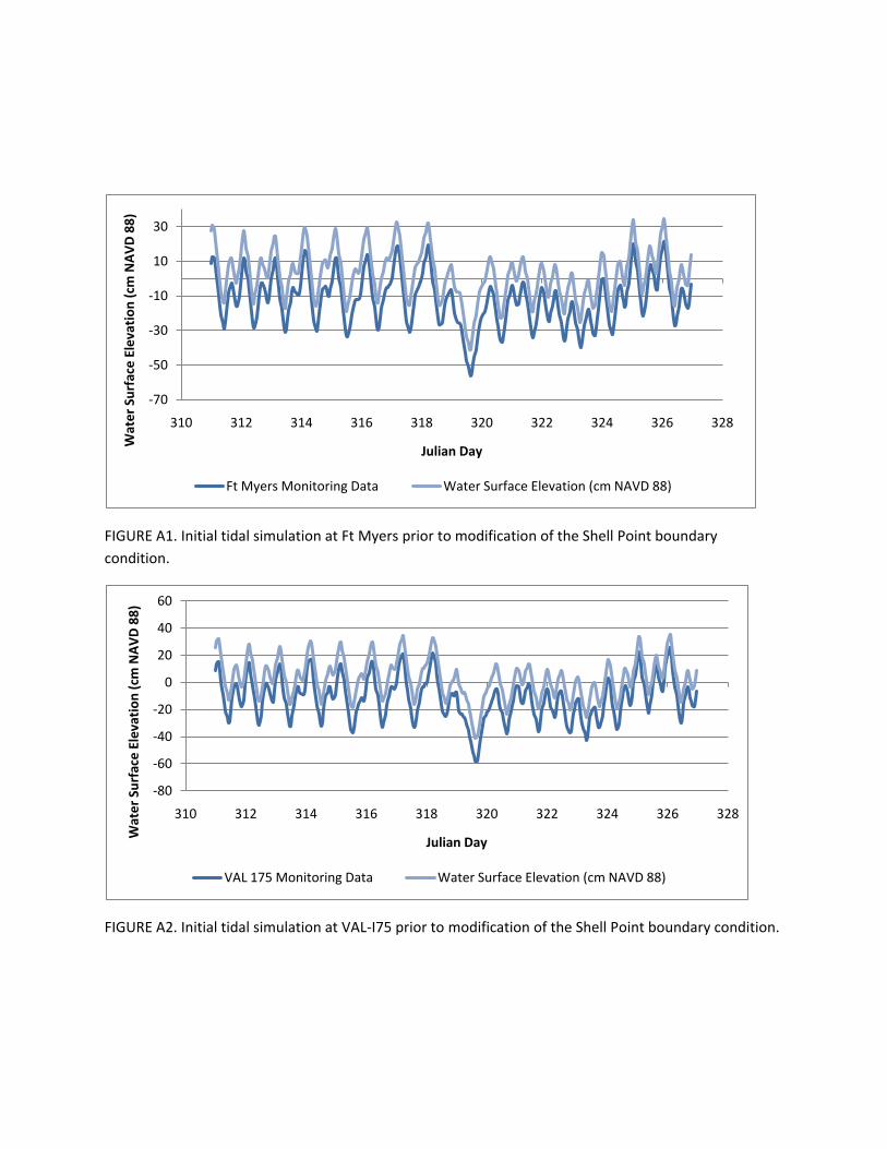
FIGURE A1. Initial tidal simulation at Ft Myers prior to modification of the Shell Point boundary condition.

FIGURE A2. Initial tidal simulation at VAL-I75 prior to modification of the Shell Point boundary condition.

-70

-50

-30

-10

10

30

310 312 314 316 318 320 322 324 326 328

Wat

er S

urfa

ce E

leva

tion

(cm

NA

VD

88)

Julian Day

Ft Myers Monitoring Data Water Surface Elevation (cm NAVD 88)

-80

-60

-40

-20

0

20

40

60

310 312 314 316 318 320 322 324 326 328

Wat

er S

urfa

ce E

leva

tion

(cm

NA

VD

88)

Julian Day

VAL 175 Monitoring Data Water Surface Elevation (cm NAVD 88)

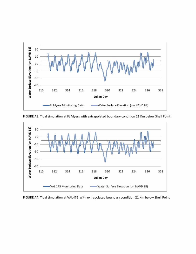
FIGURE A3. Tidal simulation at Ft Myers with extrapolated boundary condition 21 Km below Shell Point.

FIGURE A4. Tidal simulation at VAL-I75 with extrapolated boundary condition 21 Km below Shell Point

-70

-50

-30

-10

10

30

310 312 314 316 318 320 322 324 326 328

Wat

er S

urfa

ce E

leva

tion

(cm

NA

VD

88)

Julian Day

Ft Myers Monitoring Data Water Surface Elevation (cm NAVD 88)

-70

-50

-30

-10

10

30

310 312 314 316 318 320 322 324 326 328

Wat

er S

urfa

ce E

leva

tion

(cm

NA

VD

88)

Julian Day

VAL 175 Monitoring Data Water Surface Elevation (cm NAVD 88)

Attachment B

Salinity Simulation Results

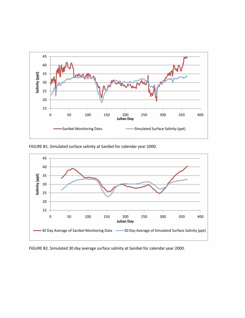
FIGURE B1. Simulated surface salinity at Sanibel for calendar year 2000.

FIGURE B2. Simulated 30 day average surface salinity at Sanibel for calendar year 2000.

15

20

25

30

35

40

45

0 50 100 150 200 250 300 350 400

Salin

ity

(ppt

)

Julian Day

Sanibel Monitoring Data Simulated Surface Salinity (ppt)

15

20

25

30

35

40

45

0 50 100 150 200 250 300 350 400

Salin

ity

(ppt

)

Julian Day

30 Day Average of Sanibel Monitoring Data 30 Day Average of Simulated Surface Salinity (ppt)

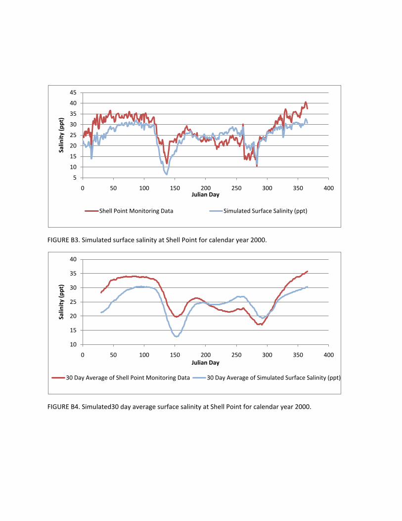
FIGURE B3. Simulated surface salinity at Shell Point for calendar year 2000.

FIGURE B4. Simulated30 day average surface salinity at Shell Point for calendar year 2000.

5

10

15

20

25

30

35

40

45

0 50 100 150 200 250 300 350 400

Salin

ity

(ppt

)

Julian Day

Shell Point Monitoring Data Simulated Surface Salinity (ppt)

10

15

20

25

30

35

40

0 50 100 150 200 250 300 350 400

Salin

ity

(ppt

)

Julian Day

30 Day Average of Shell Point Monitoring Data 30 Day Average of Simulated Surface Salinity (ppt)

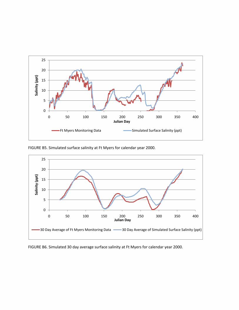
FIGURE B5. Simulated surface salinity at Ft Myers for calendar year 2000.

FIGURE B6. Simulated 30 day average surface salinity at Ft Myers for calendar year 2000.

0

5

10

15

20

25

0 50 100 150 200 250 300 350 400

Salin

ity

(ppt

)

Julian Day

Ft Myers Monitoring Data Simulated Surface Salinity (ppt)

0

5

10

15

20

25

0 50 100 150 200 250 300 350 400

Salin

ity

(ppt

)

Julian Day

30 Day Average of Ft Myers Monitoring Data 30 Day Average of Simulated Surface Salinity (ppt)

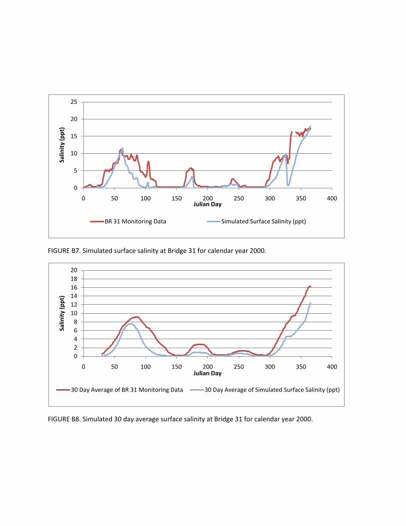
FIGURE B7. Simulated surface salinity at Bridge 31 for calendar year 2000.

FIGURE B8. Simulated 30 day average surface salinity at Bridge 31 for calendar year 2000.

0

5

10

15

20

25

0 50 100 150 200 250 300 350 400

Salin

ity

(ppt

)

Julian Day

BR 31 Monitoring Data Simulated Surface Salinity (ppt)

02468

101214161820

0 50 100 150 200 250 300 350 400

Salin

ity

(ppt

)

Julian Day

30 Day Average of BR 31 Monitoring Data 30 Day Average of Simulated Surface Salinity (ppt)

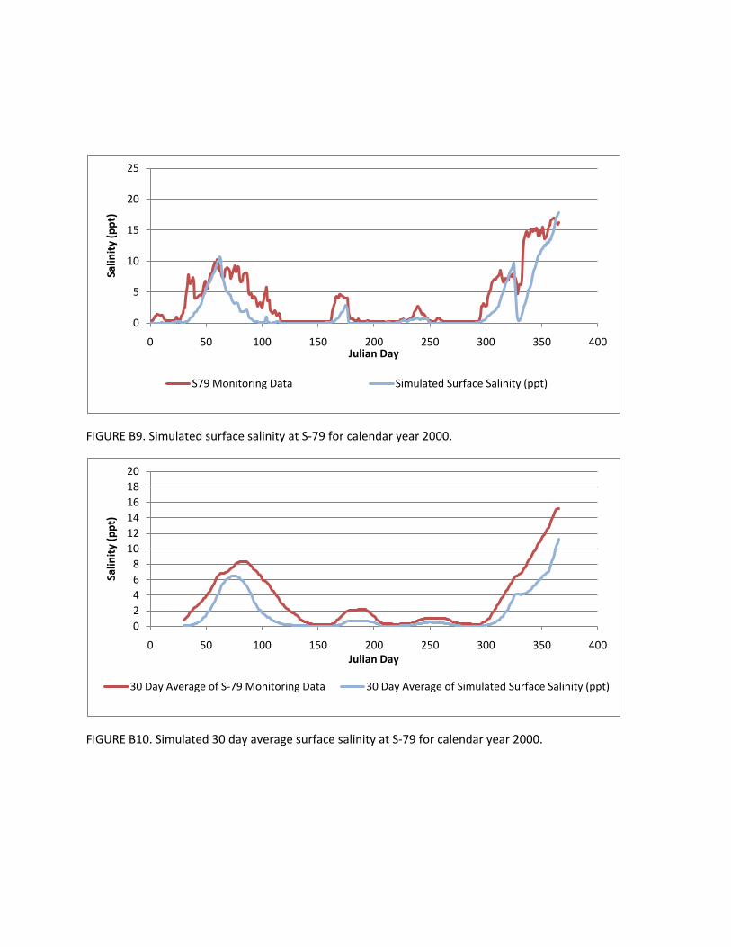
FIGURE B9. Simulated surface salinity at S-79 for calendar year 2000.

FIGURE B10. Simulated 30 day average surface salinity at S-79 for calendar year 2000.

0

5

10

15

20

25

0 50 100 150 200 250 300 350 400

Salin

ity

(ppt

)

Julian Day

S79 Monitoring Data Simulated Surface Salinity (ppt)

02468

101214161820

0 50 100 150 200 250 300 350 400

Salin

ity

(ppt

)

Julian Day

30 Day Average of S-79 Monitoring Data 30 Day Average of Simulated Surface Salinity (ppt)

Attachment C

Sea Level Rise Simulation Results

FIGURE C1. Estimation of the effects of sea level rise on the salinity distribution in the estuary with a total inflow of 14.2 m3/s at S-79.

FIGURE C2. Estimates of the effects of sea level rise on the rate of salinity increase at Ft Myers under no flow conditions.

0

5

10

15

20

25

30

35

0 5 10 15 20 25 30 35 40 45

Salin

ity

(ppt

)

Kilometers from Shell Point

Simulated Surface Salinity with 0 m SLR (ppt) Simulated Surface Salinity with 0.3 m SLR (ppt)Simulated Surface Salinity with 0.6 m SLR (ppt) Simulated Surface Salinity with 0.9 m SLR (ppt)

10

15

20

25

0 5 10 15 20

Salin

ity

(ppt

)

Time (d)

CH3D Regression of Salinity Increase at Ft Myers (ppt)Simulation of Salinity Increase at Ft Myers (ppt)Simulation of Salinity Increase at Ft Myers with 0.3 m of SLR (ppt)Simulation of Salinity Increase at Ft Myers with 0.6 m SLR (ppt)Simulation of Salinity Increase at Ft Myers with 0.9 m SLR (ppt)

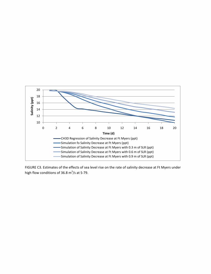
FIGURE C3. Estimates of the effects of sea level rise on the rate of salinity decrease at Ft Myers under high flow conditions of 36.8 m3/s at S-79.

10

12

14

16

18

20

0 2 4 6 8 10 12 14 16 18 20

Salin

ity

(ppt

)

Time (d)

CH3D Regression of Salinity Decrease at Ft Myers (ppt)Simulation fo Salinity Decrease at Ft Myers (ppt)Simulation of Salinity Decrease at Ft Myers with 0.3 m of SLR (ppt)Simulation of Salinity Decrease at Ft Myers with 0.6 m of SLR (ppt)Simulation of Salinity Decrease at Ft Myers with 0.9 m of SLR (ppt)