Embed Size (px)
Citation preview
FINAL REPORT OF SPECIFIC PURPOSE LIDAR SURVEY
LiDAR, Breaklines and Contours for
Suwannee River Water Management District, Florida
Add-On Agreement to
State of Florida
Division of Emergency Management
Contract 07-HS-34-14-00-22-469
January 19, 2009
Prepared by:
Dewberry 8401 Arlington Blvd.
Fairfax, VA 22031-4666 for
Program & Data Solutions (PDS) 1625 Summit Lake Drive, Suite 200
Tallahassee, FL 32317

i
Final Report of Specific Purpose LiDAR Survey, including
LiDAR-Generated Breaklines and Contours for the Suwannee River Water Management District (SRWMD), Florida
Add-On Agreement to
FDEM Contract 07-HS-34-14-00-22-469
For: Suwannee River Water Management District
c/o Paul Buchanan, GIS Coordinator Suwannee River Water Management District
9225 County Road 49 Live Oak, Florida 32060
In Coordination With:
State of Florida Division of Emergency Management
2555 Shumard Oak Blvd. Tallahassee, FL 32399
By:
Program & Data Solutions (PDS) 1625 Summit Lake Drive, Suite 200
Tallahassee, FL 32317
Prepared by: David F. Maune, PhD, PSM, PS, GS, CP, CFM
Florida Professional Surveyor and Mapper No. LS6659 Dewberry
8401 Arlington Blvd. Fairfax, VA 22031
ii
Table of Contents
Type of Survey: Specific Purpose Survey ...................................................................................... 3
The PDS Team ................................................................................................................................ 3 Name of Company in Responsible Charge ..................................................................................... 4 Name of Responsible Surveyor ...................................................................................................... 4 Survey Area .................................................................................................................................... 4 Map Reference ................................................................................................................................ 4
Summary of FDEM Baseline Specifications .................................................................................. 4 Acronyms and Definitions .............................................................................................................. 8 Ground Surveys and Dates.............................................................................................................. 9
LiDAR Aerial Survey Areas and Dates .......................................................................................... 9 LiDAR Processing Methodology .................................................................................................... 9 LiDAR Vertical Accuracy Testing ................................................................................................. 9
LiDAR Horizontal Accuracy Testing ........................................................................................... 10 LiDAR Qualitative Assessments .................................................................................................. 11
Breakline Production Methodology .............................................................................................. 12 Contour Production Methodology ................................................................................................ 12 Breakline Qualitative Assessments ............................................................................................... 18
Contour Qualitative Assessments ................................................................................................. 19 Deliverables .................................................................................................................................. 19
References ..................................................................................................................................... 20 General Notes................................................................................................................................ 21 List of Appendices ........................................................................................................................ 23
Appendix A: County Project Tiling Footprint: ........................................................................... 24
Appendix B: Geodetic Control Point BD0832 ............................................................................ 26 Appendix C: Data Dictionary ...................................................................................................... 27 Appendix D: LiDAR Processing Report...................................................................................... 51
Appendix E: QA/QC Checkpoints and Associated Discrepancies .............................................. 83 Appendix F: LiDAR Vertical Accuracy Report .......................................................................... 85
Appendix G: LiDAR Qualitative Assessment Report ................................................................. 94 Appendix H: Breakline/Contour Qualitative Assessment Report ............................................. 103
Appendix I: Geodatabase Structure ........................................................................................... 110
3
Report of Specific Purpose LiDAR Survey, LiDAR-Generated Breaklines and Contours
Suwannee River Water Management District, Florida
Type of Survey: Specific Purpose Survey
This report pertains to a Specific Purpose LiDAR Survey for the Suwannee River Water Management
District (SRWMD), Florida. The LiDAR aerial acquisition was conducted in January of 2008, and the
breaklines and contours were subsequently generated by the Program and Data Solutions (PDS) team.
The PDS team is under contract 07-HS-34-14-00-22-469 with the Florida Division of Emergency
Management (FDEM) and offered LiDAR and derived products to add-on clients, including the
SRWMD, at the same volume-discount unit rates per tile as negotiated for the FDEM contract and
utilizing the same Baseline Specifications from FDEM.
The LiDAR dataset for the SRWMD was acquired by Terrapoint USA in January of 2008 and processed
to a bare-earth digital terrain model (DTM); it was produced to FDEM Baseline Specifications. Detailed
breaklines and contours were produced by the PDS team for the 65-tile area to be mapped. Each tile
covers an area of 5000 ft by 5000 ft. The map at Appendix A displays the 65 tiles of the SRWMD for
which LiDAR DTMs and LiDAR-derived breaklines and contours were produced by the PDS team.
The FDEM Baseline Specifications require a maximum LiDAR post spacing of 4 feet, i.e., an average
point density of less than 1 point per square meter. However, the PDS team required a much higher point
density of its subcontractors in order to increase the probability of penetrating dense foliage; with nominal
post spacing of 0.7 meters per flight line and 50% sidelap between flight lines, the average point density
is 4 points per square meter. With higher point density there is a greater probability of penetrating dense
vegetation and minimizing areas defined as “low confidence areas.”
The PDS Team
PDS is a Joint Venture consisting of PBS&J, Dewberry, and URS Corp:
PBS&J provided local client liaison in Tallahassee. PBS&J was also responsible for the overall
ground survey effort including management of field survey subcontractors Allen Nobles &
Associates, Inc. (ANA) and Diversified Design & Drafting Services, Inc. (3DS) which
performed the quality assurance/quality control (QA/QC) checkpoint surveys used for
independent accuracy testing by Dewberry and URS. Mr. Glenn Bryan, PSM, of PBS&J, and
Mr. Brett Wood, PSM, of 3DS, were the technical leads for the QA/QC surveys.
Dewberry was responsible for the overall Work Plan and aerial survey effort, including
management of LiDAR subcontractors that performed the LiDAR data acquisition and post-
processing and produced LAS classified data. A staff of QA/QC specialists at Dewberry‟s office
in Tampa, FL performed quality assessments of the breaklines and contours. Dewberry served as
the single point of contact with FDEM and the add-on clients. Dr. David Maune, PSM, was
Dewberry‟s technical lead for the digital orthophoto and LiDAR surveys and derived products.
4
URS Corp. was responsible for data management and information management. URS developed
the GeoCue Distributed Production Management System (DPMS), managed and tracked the flow
of data, performed independent accuracy testing and quality assessments of FDEM‟s new LiDAR
data acquired in 2007, tracked and reported the status of individual tiles during production, and
produced all final deliverables for FDEM. Mr. Robert Ryan, CP, of URS, was the technical lead
for this effort.
Name of Company in Responsible Charge Dewberry
8401 Arlington Blvd.
Fairfax, VA 22031-4666
Name of Responsible Surveyor David F. Maune, PhD, PSM, PS, GS, CP, CFM
Florida Professional Surveyor and Mapper (PSM) No. LS6659
Survey Area The project area for this report encompasses 65 tiles, approximately 58.3 square miles, within the
Suwannee River Water Management District (SRWMD).
Map Reference There are no hardcopy map sheets for this project. The map at Appendix A provides graphical reference
to the 5000-ft x 5000-ft tiles covered by this report.
Summary of FDEM Baseline Specifications
All new data produced for the referenced contracts are required to satisfy the Florida Baseline
Specifications included as appendices to PDS‟s Task Order C from FDEM, dated August 15, 2007, and
Task Order D from FDEM, dated December 14, 2007. The tiling scheme, shown at Appendix A, is based
on the Florida State Plane Coordinate System, North Zone.
The Florida Baseline Specifications required the LiDAR data to be collected using an approved sensor
with a maximum field of view (FOV) of 20˚ on either side of nadir, with GPS baseline distances limited
to 20 miles, with maximum post spacing of 4 feet in unobscured areas for random point data, and with
vertical root mean square error (RMSEz) ≤ 0.30 ft and Fundamental Vertical Accuracy (FVA) ≤ 0.60 ft at
the 95% confidence level in open terrain (bare-earth and low grass); this accuracy is equivalent to 1 ft
contours in open terrain when tested in accordance with the National Map Accuracy Standard (NMAS).
In other land cover categories (brush lands and low trees, forested areas fully covered by trees, and urban
areas), the Florida Baseline Specifications required the LiDAR data‟s RMSEz to be ≤ 0.61 ft with
Supplemental Vertical Accuracy (SVA) and Consolidated Vertical Accuracy (CVA) ≤ 1.19 ft at the 95%
confidence level; this accuracy is equivalent to 2 ft contours when tested in accordance with the NMAS.
Low confidence areas, originally called obscured vegetated areas, are defined for areas where the vertical
data may not meet the data accuracy requirements due to heavy vegetation.
The Florida Baseline Specifications also require the horizontal accuracy to meet or exceed 3.8 feet at the
95% confidence level, using RMSEr x 1.7308. This means that the horizontal (radial) RMSE (RMSEr)
must meet or exceed 2.20 ft. This is the horizontal accuracy required of maps compiled at a scale of
1:1,200 (1” = 100‟) in accordance with the traditional National Map Accuracy Standard.
5
To meet and exceed these specifications, the PDS team established the following more-rigorous
specifications for its LiDAR subcontractors:
Instead of a 20˚ FOV on either side of nadir, the PDS team limited the FOV to 18˚
Instead of GPS baselines ≤ 20 miles, the PDS team limited baseline lengths to ≤ 20 km, except in
one small isolated area where the baseline length was approximately 23 km (14 miles).
Instead of 4 foot post spacing which yields an average of 0.67 points per m2, the PDS team chose
0.7 m point spacing and 50% sidelap that yields an average of 4 points per m2. Thus, the PDS
team‟s average point density is nearly 6 times higher than required by FDEM, greatly increasing
the probability of LiDAR points penetrating through dense vegetation so as to minimize areas
defined as low confidence areas. The PDS team defines low confidence areas as vegetated areas
of ½ acre or larger that are considered obscured to the extent that adequate vertical data cannot be
clearly determined to accurately define the DTM. Such areas indicate where the vertical data
may not meet the data accuracy requirements due to heavy vegetation.
The first deliverable is LiDAR mass points, delivered to LAS 1.1 specifications, including the following
LAS classification codes:
Class 1 = Unclassified, and used for all other features that do not fit into the Classes 2, 7, 9, or 12,
including vegetation, buildings, etc.
Class 2 = Ground, includes accurate LiDAR points in overlapping flight lines
Class 7 = Noise, includes LiDAR points in overlapping flight lines
Class 9 = Water, includes LiDAR points in overlapping flight lines
Class 12 = Overlap, including areas of overlapping flight lines which have been deliberately
removed from Class 1 because of their reduced accuracy.
Per FDEM‟s Baseline Specifications, for each 500 square mile area, a total of 120 “blind” QA/QC
checkpoints were surveyed, totally unknown to (i.e., “blind” from) the LiDAR subcontractor. Each set of
120 QA/QC checkpoints had the goal to include 30 checkpoints in each of the following four land cover
categories:
Category 1 = bare-earth and low grass
Category 2 = brush lands and low trees
Category 3 = forested areas fully covered by trees
Category 4 = urban areas
Because the 65 tiles for the SRWMD only encompassed 58 square miles instead of 500 square miles, only
11.6% of the normal 30 points per category (less than one point per category) is required. A total of 23
QA/QC checkpoints were used, as listed at Appendix E.
The following vertical accuracy guidelines were specified by the Florida Baseline Specifications:
In category 1, the RMSEz must be ≤ 0.30 ft (Accuracyz ≤ 0.60 ft at the 95% confidence level);
Accuracyz in Category 1 refers to Fundamental Vertical Accuracy (FVA) which defines how
accurate the elevation data are when not complicated by asphalt or vegetation that may cause
6
elevations to be either lower or higher than the bare earth terrain. This is equivalent to the
accuracy expected of 1 ft contours in non-vegetated terrain.
In category 2, the RMSEz must be ≤ 0.61 ft (Accuracyz ≤ 1.19 ft at the 95% confidence level);
Accuracyz in Category 2 refers to Supplemental Vertical Accuracy (SVA) in brush lands and low
trees and defines how accurate the elevation data are when complicated by such vegetation that
frequently causes elevations to higher than the bare earth terrain. This is equivalent to the
accuracy expected of 2 ft contours in such terrain.
In category 3, the RMSEz must be ≤ 0.61 ft (Accuracyz ≤ 1.19 ft at the 95% confidence level);
Accuracyz in Category 3 refers to Supplemental Vertical Accuracy (SVA) in forested areas fully
covered by trees and defines how accurate the elevation data are when complicated by such
vegetation that frequently causes elevations to be higher than the bare earth terrain. This is
equivalent to the accuracy expected of 2 ft contours in such terrain.
In category 4, the RMSEz must be ≤ 0.61 ft (Accuracyz ≤ 1.19 ft at the 95% confidence level);
Accuracyz in Category 4 refers to Supplemental Vertical Accuracy (SVA) in urban areas typically
paved with asphalt and defines how accurate the elevation data are when complicated by asphalt
that frequently causes elevations to be lower than the bare earth terrain. This is equivalent to the
accuracy expected of 2 ft contours in such terrain.
In all land cover categories combined, the RMSEz must be ≤ 0.61 ft (Accuracyz ≤ 1.19 ft at the
95% confidence level); Accuracyz in all categories combined refers to Consolidated Vertical
Accuracy (CVA).
The terms FVA, SVA and CVA are explained in Chapter 3, Accuracy Standards & Guidelines, of
“Digital Elevation Model Technologies and Applications: The DEM Users Manual,” published
by the American Society for Photogrammetry and Remote Sensing (ASPRS), January, 2007.
A second major deliverable consists of nine types of breaklines, produced in accordance with the PDS
team‟s Data Dictionary at Appendix C:
1. Coastal shoreline features
2. Single-line hydrographic features
3. Dual-line hydrographic features
4. Closed water body features
5. Road edge-of-pavement features
6. Bridge and overpass features
7. Soft breakline features
8. Island features
9. Low confidence areas
Another major deliverable includes both one-foot and two-foot contours, produced from the mass points
and breaklines, certified to meet or exceed NSSDA standards for one-foot contours. Two-foot contours
within obscured vegetated areas are not required to meet NSSDA standards. These contours were also
produced in accordance with the PDS team‟s Data Dictionary at Appendix C.
Table 1 is included below for ease in understanding the accuracy requirements when comparing the
traditional National Map Accuracy Standard (NMAS) and the newer National Standard for Spatial Data
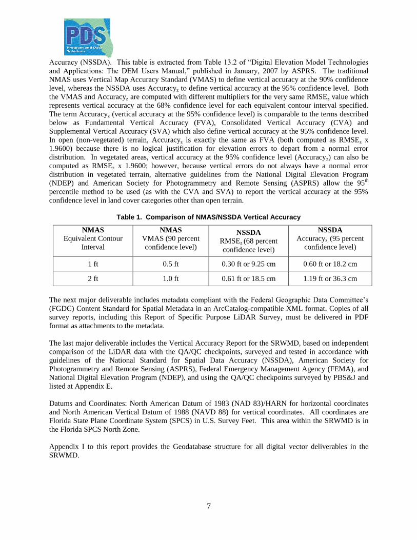
7
Accuracy (NSSDA). This table is extracted from Table 13.2 of “Digital Elevation Model Technologies
and Applications: The DEM Users Manual,” published in January, 2007 by ASPRS. The traditional
NMAS uses Vertical Map Accuracy Standard (VMAS) to define vertical accuracy at the 90% confidence
level, whereas the NSSDA uses Accuracyz to define vertical accuracy at the 95% confidence level. Both
the VMAS and Accuracyz are computed with different multipliers for the very same RMSEz value which
represents vertical accuracy at the 68% confidence level for each equivalent contour interval specified.
The term Accuracyz (vertical accuracy at the 95% confidence level) is comparable to the terms described
below as Fundamental Vertical Accuracy (FVA), Consolidated Vertical Accuracy (CVA) and
Supplemental Vertical Accuracy (SVA) which also define vertical accuracy at the 95% confidence level.
In open (non-vegetated) terrain, Accuracyz is exactly the same as FVA (both computed as RMSEz x
1.9600) because there is no logical justification for elevation errors to depart from a normal error
distribution. In vegetated areas, vertical accuracy at the 95% confidence level (Accuracyz) can also be
computed as RMSEz x 1.9600; however, because vertical errors do not always have a normal error
distribution in vegetated terrain, alternative guidelines from the National Digital Elevation Program
(NDEP) and American Society for Photogrammetry and Remote Sensing (ASPRS) allow the 95th
percentile method to be used (as with the CVA and SVA) to report the vertical accuracy at the 95%
confidence level in land cover categories other than open terrain.
Table 1. Comparison of NMAS/NSSDA Vertical Accuracy
NMAS
Equivalent Contour
Interval
NMAS
VMAS (90 percent
confidence level)
NSSDA
RMSEz (68 percent
confidence level)
NSSDA
Accuracyz, (95 percent
confidence level)
1 ft 0.5 ft 0.30 ft or 9.25 cm 0.60 ft or 18.2 cm
2 ft 1.0 ft 0.61 ft or 18.5 cm 1.19 ft or 36.3 cm
The next major deliverable includes metadata compliant with the Federal Geographic Data Committee‟s
(FGDC) Content Standard for Spatial Metadata in an ArcCatalog-compatible XML format. Copies of all
survey reports, including this Report of Specific Purpose LiDAR Survey, must be delivered in PDF
format as attachments to the metadata.
The last major deliverable includes the Vertical Accuracy Report for the SRWMD, based on independent
comparison of the LiDAR data with the QA/QC checkpoints, surveyed and tested in accordance with
guidelines of the National Standard for Spatial Data Accuracy (NSSDA), American Society for
Photogrammetry and Remote Sensing (ASPRS), Federal Emergency Management Agency (FEMA), and
National Digital Elevation Program (NDEP), and using the QA/QC checkpoints surveyed by PBS&J and
listed at Appendix E.
Datums and Coordinates: North American Datum of 1983 (NAD 83)/HARN for horizontal coordinates
and North American Vertical Datum of 1988 (NAVD 88) for vertical coordinates. All coordinates are
Florida State Plane Coordinate System (SPCS) in U.S. Survey Feet. This area within the SRWMD is in
the Florida SPCS North Zone.
Appendix I to this report provides the Geodatabase structure for all digital vector deliverables in the
SRWMD.
8
Acronyms and Definitions 3DS Diversified Design & Drafting Services, Inc.
Accuracyr Horizontal (radial) accuracy at the 95% confidence level, defined by the NSSDA
Accuracyz Vertical accuracy at the 95% confidence level, defined by the NSSDA
ANA Allen Nobles & Associates, Inc.
ASFPM Association of State Floodplain Managers
ASPRS American Society for Photogrammetry and Remote Sensing
CFM Certified Floodplain Manager (ASFPM)
CMAS Circular Map Accuracy Standard, defined by the NMAS
CP Certified Photogrammetrist (ASPRS)
CVA Consolidated Vertical Accuracy, defined by the NDEP and ASPRS
DEM Digital Elevation Model (gridded DTM)
DTM Digital Terrain Model (mass points and breaklines to map the bare earth terrain)
DSM Digital Surface Model (top reflective surface, includes treetops and rooftops)
FDEM Florida Division of Emergency Management
FEMA Federal Emergency Management Agency
FGDC Federal Geographic Data Committee
FOV Field of View
FVA Fundamental Vertical Accuracy, defined by the NDEP and ASPRS
GS Geodetic Surveyor
LAS LiDAR data format as defined by ASPRS
LiDAR Light Detection and Ranging
MHHW Mean Higher High Water
MHW Mean High Water, defines official shoreline in Florida
MLLW Mean Lower Low Water
MLW Mean Low Water
MSL Mean Sea Level
NAD 83 North American Datum of 1983
NAVD 88 North American Vertical Datum of 1988
NDEP National Digital Elevation Program
NMAS National Map Accuracy Standard
NOAA National Oceanic and Atmospheric Administration
NSSDA National Standard for Spatial Data Accuracy
NSRS National Spatial Reference System
NWFWMD Northwest Florida Water Management District
PDS Program & Data Solutions, joint venture between PBS&J, Dewberry and URS Corp
PS Photogrammetric Surveyor
PSM Professional Surveyor and Mapper (Florida)
QA/QC Quality Assurance/Quality Control
RMSEh Vertical Root Mean Square Error (RMSE) of ellipsoid heights
RMSEr Horizontal (radial) Root Mean Square Error (RMSE) computed from RMSEx and RMSEy
RMSEz Vertical Root Mean Square Error (RMSE) of orthometric heights
SLOSH Sea, Lake, and Overland Surges from Hurricanes
SRWMD Suwannee River Water Management District SVA Supplemental Vertical Accuracy, defined by the NDEP and ASPRS
TIN Triangulated Irregular Network
VMAS Vertical Map Accuracy Standard, defined by the NMAS
9
Ground Surveys and Dates
The GPS ground checkpoint surveys were executed on March 31, 2008.
The QA/QC checkpoints used for this county are listed at Appendix E.
LiDAR Aerial Survey Areas and Dates Terrapoint USA collected the LiDAR data for the SRWMD during January of 2008.
LiDAR Processing Methodology A LiDAR processing report from Terrapoint USA is included at Appendix D.
LiDAR Vertical Accuracy Testing
URS performed the LiDAR vertical accuracy assessment for the SRWMD. Because there were fewer
than 20 QA/QC checkpoints for this small area, normal procedures could not be used for accuracy testing
in accordance with ASPRS Guidelines, Vertical Accuracy Reporting for Lidar Data, May 24, 2004, and
Section 1.5 of the Guidelines for Digital Elevation Data, published by the National Digital Elevation
Program (NDEP), May 10, 2004. These guidelines call for the mandatory determination of Fundamental
Vertical Accuracy (FVA) and Consolidated Vertical Accuracy (CVA), and the optional determination of
Supplemental Vertical Accuracy (SVA).
Using alternative procedures described below, the LiDAR dataset of the SRWMD passed the accuracy
testing by URS as documented at Appendices E and F.
Fundamental Vertical Accuracy (FVA) is determined with QA/QC checkpoints located only in open
terrain (grass, dirt, sand, and rocks) where there is a high probability that the LiDAR sensor detected the
bare-earth ground surface, and where errors are expected to follow a normal error distribution. With a
normal error distribution, the FVA at the 95 percent confidence level is computed as the vertical root
mean square error (RMSEz) of the checkpoints x 1.9600. The FVA is the same as Accuracyz at the 95%
confidence level (for open terrain), as specified in Appendix 3-A of the National Standard for Spatial
Data Accuracy, FGDC-STD-007.3-1998, see http://www.fgdc.gov/standards/projects/FGDC-standards-
projects/accuracy/part3/chapter3. For FDEM, the FVA standard is .60 feet at the 95% confidence level,
corresponding to an RMSEz of 0.30 feet or 9.25 cm, the accuracy expected from 1-foot contours. In the
SRWMD area, the RMSEz in open terrain equaled 0.25 ft compared with the 0.30 ft specification of
FDEM; and the FVA computed using RMSEz x 1.9600 was equal to 0.49 ft compared with the 0.60 ft
specification of FDEM.
Consolidated Vertical Accuracy (CVA) is determined with all checkpoints, representing open terrain
and all other land cover categories combined. If errors follow a normal error distribution, the CVA can be
computed by multiplying the consolidated RMSEz by 1.9600. However, because bare-earth elevation
errors often vary based on the height and density of vegetation, a normal error distribution cannot be
assumed, and RMSEz cannot necessarily be used to calculate the 95 percent confidence level. Instead, a
nonparametric testing method, based on the 95th percentile, may be used to determine CVA at the 95
percent confidence level. NDEP guidelines state that errors larger than the 95th percentile should be
documented in the quality control report and project metadata. For FDEM, the CVA specification for all
10
classes combined should be less than or equal to 1.19 feet; this same CVA specification was used by
NOAA. In the SRWMD, the CVA computed using RMSEz x 1.9600 was equal to .61 ft, compared with
the 1.19 ft specification of FDEM; and the CVA computed using the 95th
percentile was equal to 0.57
ft. The SRWMD dataset passed the CVA standard.
Supplemental Vertical Accuracy (SVA) is determined separately for each individual land cover
category, recognizing that the LiDAR sensor and post-processing may not have mapped the bare-earth
ground surface, and that errors may not follow a normal error distribution. SVA specifications are
“target” values and not mandatory, recognizing that larger errors in some categories are offset by smaller
errors in other land cover categories, so long as the overall mandatory CVA specification is satisfied. For
each land cover category, the SVA at the 95 percent confidence level equals the 95th percentile error for
all checkpoints in that particular land cover category. For FDEM‟s specification, the SVA target is 1.19
feet for each category; this same SVA target specification was used by NOAA. In the SRWMD the SVA
tested as 0.37 ft in open terrain, bare earth and low grass; 0.18 ft in brush lands and low trees; 0.66 ft
in forested areas; and 0.56 ft in urban, built-up areas, passing the FDEM SVA baseline target
specification of 1.19 ft in all land cover categories.
The complete LiDAR Vertical Accuracy Report for the SRWMD is at Appendix F.
LiDAR Horizontal Accuracy Testing The LiDAR data was compiled to meet 3.8 feet horizontal accuracy at the 95% confidence level.
Whereas FDEM baseline specifications call for horizontal accuracy testing, traditional horizontal
accuracy testing of LiDAR data is not cost effective for the following reasons:
Paragraphs 3.2.2 and 3.2.3 of the National Standard for Spatial Data Accuracy (NSSDA) states:
“Horizontal accuracy shall be tested by comparing the planimetric coordinates of well-defined
points in the dataset with coordinates of the same points from an independent source of higher
accuracy … when a dataset, e.g., a gridded digital elevation dataset or elevation contour dataset
does not contain well-defined points, label for vertical accuracy only.” Similarly, in Appendix 3-
C of the NSSDA, paragraph 1 explains well-defined points as follows: “A well-defined point
represents a feature for which the horizontal position is known to a high degree of accuracy and
position with respect to the geodetic datum. For the purpose of accuracy testing, well-defined
points must be easily visible or recoverable on the ground, on the independent source of higher
accuracy, and on the product itself. Graphic contour data and digital hypsographic data may not
contain well-defined points.”
Paragraph 1.5.3.4 of the Guidelines for Digital Elevation Data, published in 2004 by the National
Digital Elevation Program (NDEP), states: “The NDEP does not require independent testing of
horizontal accuracy for elevation products. When the lack of distinct surface features makes
horizontal accuracy testing of mass points, TINs, or DEMs difficult or impossible, the data
producer should specify horizontal accuracy using the following statement: Compiled to meet __
(meters, feet) horizontal accuracy at 95 percent confidence level.”
Paragraph 1.2, Horizontal Accuracy, of ASPRS Guidelines, Vertical Accuracy Reporting for
Lidar Data, published by the American Society for Photogrammetry and Remote Sensing
(ASPRS) in 2004, further explains why it is difficult and impractical to test the horizontal
accuracy of LiDAR data, and explains why ASPRS does not require horizontal accuracy testing
of LiDAR-derived elevation products.
ASPRS has been actively seeking to develop cost-effective techniques to use LiDAR intensity
imagery to test the horizontal accuracy of LiDAR data. As recently as May 1, 2008, at the annual
11
conference of ASPRS, the most relevant technique for doing so was in a paper entitled “New
Horizontal Accuracy Assessment Tools and Techniques for Lidar Data,” presented by the Ohio
DOT. Whereas the technique had research value, it was neither practical nor affordable for use in
horizontal accuracy testing of FDEM data.
Appendix A of FDEM‟s Baseline Specifications require 20 horizontal test points for every 500
square mile area of digital orthophotos to be produced, and Appendix B of FDEM‟s Baseline
Specifications requires 120 vertical test points for each 500 square mile area of LiDAR data to be
produced. The PDS task orders included no funding for the more-expensive horizontal
checkpoints that would be certain to appear on LiDAR intensity images as clearly-defined point
features.
In addition to LiDAR system factory calibration of horizontal and vertical accuracy, each of the
PDS team‟s LiDAR subcontractors have different techniques for field calibration checks used to
determine if bore-sighting is still accurate. Terrapoint‟s technique, used for the SRWMD, is
explained in the LiDAR Processing Report at Appendix D.
LiDAR Qualitative Assessments In addition to vertical accuracy testing, URS also performed the LiDAR qualitative assessment.
An assessment of the vertical accuracy alone does not yield a complete picture with regard to the usability
of LiDAR data for its intended purpose. It is very possible for a given set of LiDAR data to meet the
accuracy requirements, yet still contain artifacts (non-ground points) in the bare-earth surface, or a lack of
ground points in some areas that may render the data, in whole or in part, unsuitable for certain
applications.
Based on the extremely large volume of elevation points generated, it is neither time efficient, cost
effective, nor technically practical to produce a perfectly clean (artifact-free) bare-earth terrain surface.
The purpose of the LiDAR Qualitative Assessment Report (see Appendix G) is to provide a qualitative
analysis of the “cleanliness” of the bare-earth terrain surface for use in supporting riverine and coastal
analysis, modeling, and mapping.
The main software programs used by URS in performing the bare-earth data cleanliness review include
the following:
GeoCue: a geospatial data/process management system especially suited to managing large
LiDAR data sets
TerraModeler: used for analysis and visualization
TerraScan: runs inside of MicroStation; used for point classification and points file generation
GeoCue LAS EQC: is also used for data analysis and edit
The following systematic approach was followed by URS in performing the cleanliness review and
analysis:
Uploaded data to the GeoCue data warehouse (enhanced data management)
o LiDAR: cut the data into uniform tiles measuring 5,000 feet by 5,000 feet – using the
State Plane tile index provided by FDEM
o Imagery: Best available orthophotography was used to facilitate the data review.
Additional LiDAR Orthos were created from the LiDAR intensity data and used for
review purposes.
12
Performed coverage/gap check to ensure proper coverage of the project area
o Created a large post grid (~30 meters) from the bare-earth points, which was used to
identify any holes or gaps in the data coverage.
Performed tile-by-tile analyses
o Using TerraScan and LAS EQC, checked for gross errors in profile mode (noise, high
and low points)
o Reviewed each tile for anomalies; identified problem areas with a polygon, annotated
comment, and screenshot as needed for clarification and illustration. Used ortho imagery
when necessary to aid in making final determinations with regards to:
Buildings left in the bare-earth points file
Vegetation left in the bare-earth points file
Water points left in the bare-earth points file
Proper definition of roads
Bridges and large box culverts removed from the bare-earth points file
Areas that may have been “shaved off” or “over-smoothed” during the auto-
filtering process
Prepared and sent the error reports to LiDAR firm for correction
Reviewed revisions and comments from the LiDAR firm
Prepared and submitted final reports to FDEM
Breakline Production Methodology
For the hard breaklines, Dewberry used GeoCue software to develop LiDAR stereo models of Clay and
Putnam counties so the LiDAR derived data could be viewed in 3-D stereo using Socet Set softcopy
photogrammetric software. Using LiDARgrammetry procedures with LiDAR intensity imagery,
Dewberry stereo-compiled the eight types of hard breaklines in accordance with the Data Dictionary at
Appendix C. For the soft hydro breaklines, Dewberry used 2.5-D techniques to digitize soft, linear
hydrographic features first in 2-D and then used its GeoFIRM toolkit to drape the soft breaklines over the
ESRI Terrain to derive the Z-values (elevations), also consistent with the Data Dictionary at Appendix C.
All breakline compilation was performed under the direct supervision of an ASPRS Certified
Photogrammetrist and Florida Professional Surveyor and Mapper (PSM). The breaklines conform with
data format requirements outlined by the FDEM Baseline Specifications.
Whereas flowing rivers and streams are “hydro-enforced” to depict the downward flow of water, dry
drainage features are not “hydro-enforced” but deliberately include undulations that more-accurately
represent the true topography. This is, in fact, the ideal situation for topographic mapping.
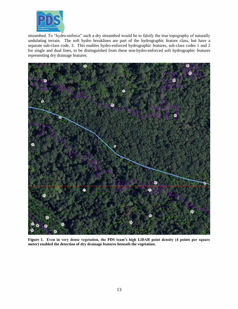
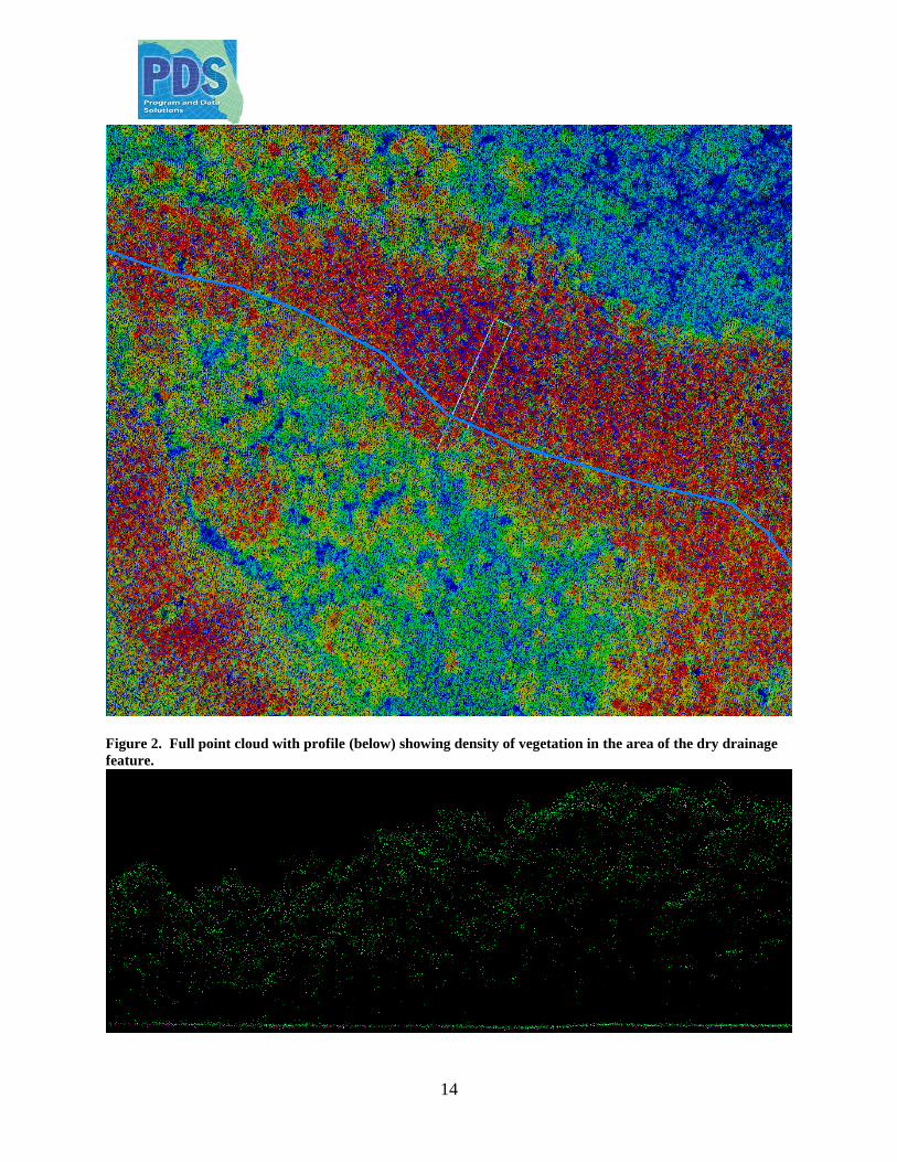
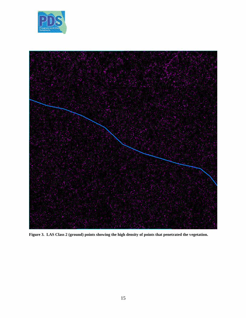
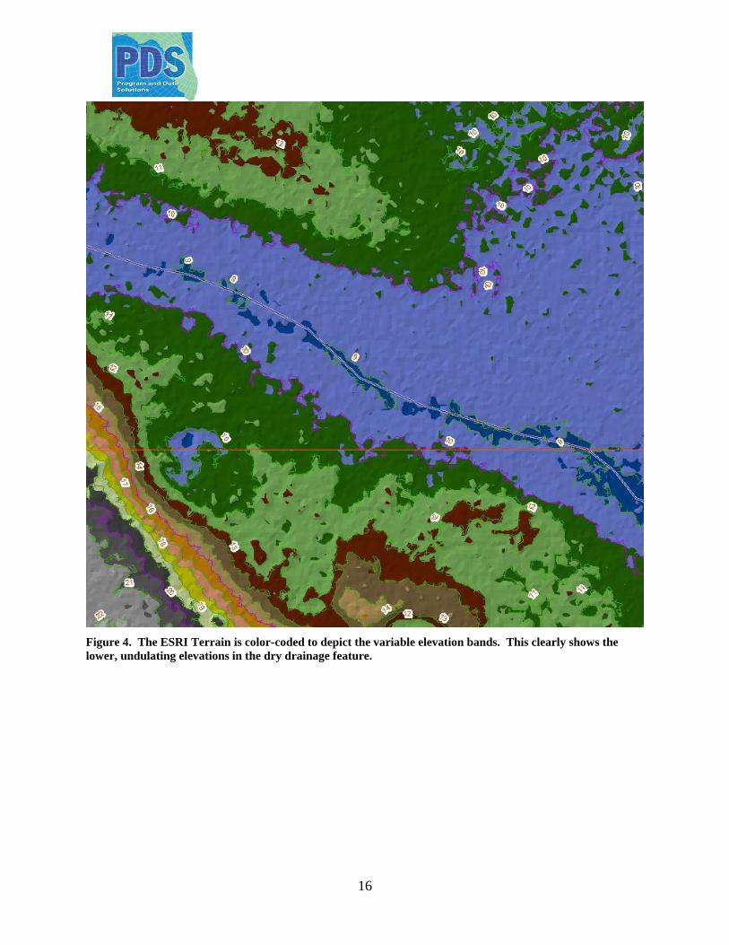
The five figures below demonstrate how the PDS team‟s high LiDAR point density (4 points per square
meter) are used to penetrate dense vegetation and accurately map the dry drainage feature not visible from
a normal digital orthophoto (Figure 1); the total density of the LiDAR point cloud (Figure 2); the density
of LAS Class 2 points that penetrated to the ground (Figure 3); the color-coded Terrain to help in
visualizing the variable elevations (Figure 4); and the soft hydro breakline that approximates the potential
flow line of the dry drainage feature and the contours that clearly show the undulations in the Terrain
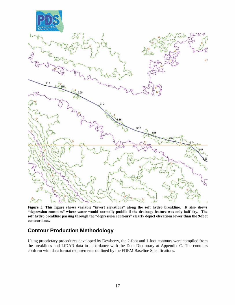
(Figure 5). At Figure 5, the 9-foot contour lines are depression contours that surround elevation points
that are lower than 9-feet. Although the undulations, by definition, are not “hydro-enforced,” the PDS
Team‟s PSM in responsible charge of this project considers it a violation of professional standards if one
were to deliberately degrade the accurate Terrain, soft hydro breakline and contours in a dry drainage
feature in order to “hydro-enforce” that feature by filling the depressions and falsely scalping off the
higher undulations in order to make an idealized monotonic dry streambed out of the true undulating
13
streambed. To “hydro-enforce” such a dry streambed would be to falsify the true topography of naturally
undulating terrain. The soft hydro breaklines are part of the hydrographic feature class, but have a
separate sub-class code, 3. This enables hydro-enforced hydrographic features, sub-class codes 1 and 2
for single and dual lines, to be distinguished from these non-hydro-enforced soft hydrographic features
representing dry drainage features.
Figure 1. Even in very dense vegetation, the PDS team’s high LiDAR point density (4 points per square
meter) enabled the detection of dry drainage features beneath the vegetation.
14
Figure 2. Full point cloud with profile (below) showing density of vegetation in the area of the dry drainage
feature.
15
Figure 3. LAS Class 2 (ground) points showing the high density of points that penetrated the vegetation.
16
Figure 4. The ESRI Terrain is color-coded to depict the variable elevation bands. This clearly shows the
lower, undulating elevations in the dry drainage feature.
17
Figure 5. This figure shows variable “invert elevations” along the soft hydro breakline. It also shows
“depression contours” where water would normally puddle if the drainage feature was only half dry. The
soft hydro breakline passing through the “depression contours” clearly depict elevations lower than the 9-foot
contour lines.
Contour Production Methodology
Using proprietary procedures developed by Dewberry, the 2-foot and 1-foot contours were compiled from
the breaklines and LiDAR data in accordance with the Data Dictionary at Appendix C. The contours
conform with data format requirements outlined by the FDEM Baseline Specifications.
18
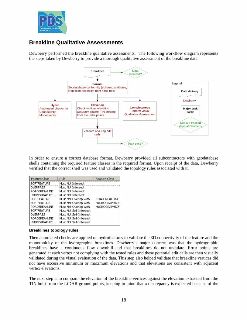
Breakline Qualitative Assessments
Dewberry performed the breakline qualitative assessments. The following workflow diagram represents
the steps taken by Dewberry to provide a thorough qualitative assessment of the breakline data.
Hydro
Automated checks for
Connectivity,
Monotonicity
Elevation
Check vertices elevation
accuracy against TIN created
from the Lidar points
Completeness
Perform visual
Qualitative Assessment
Breaklines
Format
Geodatabase conformity (schema, attributes,
projection, topology, right hand rule)
Data
received?
Geocue tracked
steps at Dewberry
Data pass?
Validate and Log edit
calls
Major task
Tasks
Dewberry
Legend
Data delivery
In order to ensure a correct database format, Dewberry provided all subcontractors with geodatabase
shells containing the required feature classes in the required format. Upon receipt of the data, Dewberry
verified that the correct shell was used and validated the topology rules associated with it.
Breaklines topology rules
Then automated checks are applied on hydrofeatures to validate the 3D connectivity of the feature and the
monotonicity of the hydrographic breaklines. Dewberry‟s major concern was that the hydrographic
breaklines have a continuous flow downhill and that breaklines do not undulate. Error points are
generated at each vertex not complying with the tested rules and these potential edit calls are then visually
validated during the visual evaluation of the data. This step also helped validate that breakline vertices did
not have excessive minimum or maximum elevations and that elevations are consistent with adjacent
vertex elevations.
The next step is to compare the elevation of the breakline vertices against the elevation extracted from the
TIN built from the LiDAR ground points, keeping in mind that a discrepancy is expected because of the
19
hydro-enforcement applied to the breaklines and because of the interpolated imagery used to acquire the
breaklines. A given tolerance is used to validate if the elevations do not differ too much from the LiDAR.
Dewberry‟s final check for the breaklines was to perform a full qualitative analysis of the breaklines.
Dewberry compared the breaklines against LiDAR intensity images to ensure breaklines were captured in
the required locations.
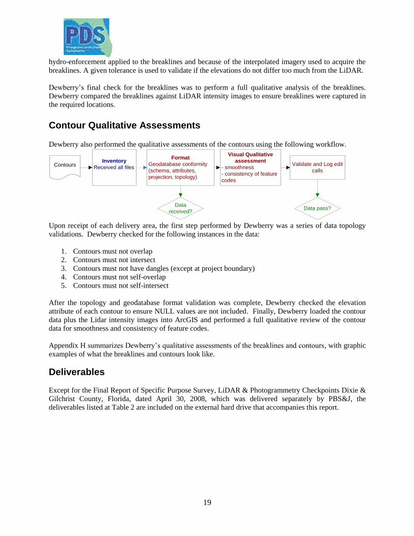
Contour Qualitative Assessments Dewberry also performed the qualitative assessments of the contours using the following workflow.
Contours
Format
Geodatabase conformity
(schema, attributes,
projection, topology)
Visual Qualitative
assessment
- smoothness
- consistency of feature
codes
Validate and Log edit
calls
Data
received?Data pass?
Inventory
Received all files
Upon receipt of each delivery area, the first step performed by Dewberry was a series of data topology
validations. Dewberry checked for the following instances in the data:
1. Contours must not overlap
2. Contours must not intersect
3. Contours must not have dangles (except at project boundary)
4. Contours must not self-overlap
5. Contours must not self-intersect
After the topology and geodatabase format validation was complete, Dewberry checked the elevation
attribute of each contour to ensure NULL values are not included. Finally, Dewberry loaded the contour
data plus the Lidar intensity images into ArcGIS and performed a full qualitative review of the contour
data for smoothness and consistency of feature codes.
Appendix H summarizes Dewberry‟s qualitative assessments of the breaklines and contours, with graphic
examples of what the breaklines and contours look like.
Deliverables
Except for the Final Report of Specific Purpose Survey, LiDAR & Photogrammetry Checkpoints Dixie &
Gilchrist County, Florida, dated April 30, 2008, which was delivered separately by PBS&J, the
deliverables listed at Table 2 are included on the external hard drive that accompanies this report.
20
Table 2. Summary of Deliverables
Copies Deliverable Description Format Location
2 Final Report of Specific Purpose Survey, LiDAR
& Photogrammetry Checkpoints, Dixie &
Gilchrist County, Florida, dated April 30, 2008
Hardcopy and pdf Submitted separately
1 Data Dictionary pdf Appendix C
3 LiDAR Processing Report Hardcopy and pdf Appendix D
3 LiDAR Vertical Accuracy Report Hardcopy and pdf Appendix F
1 LiDAR Qualitative Assessment Report pdf Appendix G
1 Breakline/Contour Qualitative Assessment Report pdf Appendix H
1 Breaklines, Contours, Network-Adjusted Control
Points, Vertical accuracy checkpoints, Tiling
Footprint, Lidar ground masspoints
Geodatabase Submitted separately
References ASPRS, 2007, Digital Elevation Model Technologies and Applications: The DEM Users Manual, 2
nd
edition, American Society for Photogrammetry and Remote Sensing, Bethesda, MD.
ASPRS, 2004, ASPRS Guidelines, Vertical Accuracy Reporting for Lidar Data, American Society for
Photogrammetry and Remote Sensing, Bethesda, MD, May 24, 2004, http://www.asprs.org/society/
committees/lidar/downloads/Vertical_Accuracy_Reporting_for_Lidar_Data.pdf.
Bureau of the Budget, 1947, National Map Accuracy Standards, Office of Management and Budget,
Washington, D.C.
FDEM, 2006, Florida GIS, Baseline Specifications for Orthophotography and LiDAR, Appendix B,
Terrestrial LiDAR Specifications, Florida Division of Emergency Management, Tallahassee, FL, October,
2006.
FEMA, 2004, Appendix A, Guidance for Aerial Mapping and Surveying, to “Guidelines and
Specifications for Flood Hazard Mapping Partners,” Federal Emergency Management Agency,
Washington, D.C. FGCC, 1984, Standards and Specifications for Geodetic Control Networks, Federal Geodetic Control
Committee, Silver Spring, ,MD, reprinted August 1993.
FGCC, 1988, Geometric Geodetic Accuracy Standards and Specifications for Using GPS Relative
Positioning Techniques, Federal Geodetic Control Committee, Silver Spring, MD, reprinted with
corrections, August, 1989.
FGDC, 1998a, Geospatial Positioning Accuracy Standards, Part I: Reporting Methodology, Federal
Geographic Data Committee, c/o USGS, Reston, VA,
http://www.fgdc.gov/standards/standards_publications/.
21
FGDC, 1998b, Geospatial Positioning Accuracy Standards, Part 2, Standards for Geodetic Networks,
Federal Geographic Data Committee, c/o USGS, Reston, VA,
http://www.fgdc.gov/standards/standards_publications/
FGDC, 1998b, Geospatial Positioning Accuracy Standards, Part 3, National Standard for Spatial Data
Accuracy, Federal Geographic Data Committee, c/o USGS, Reston, VA,
http://www.fgdc.gov/standards/standards_publications/
FGDC, 1998d, Content Standard for Digital Geospatial Metadata (CSDGM), Federal Geographic Data
Committee, c/o USGS, Reston, VA, www.fgdc.gov/metadata/contstan.html.
NDEP, 2004, Guidelines for Digital Elevation Data, Version 1.0, National Digital Elevation Program,
May 10, 2004, http://www.ndep.gov/
NOAA, 1997, Guidelines for Establishing GPS-Derived Ellipsoid Heights (Standards: 2 cm and 5 cm),
NOAA Technical Memorandum NOS NGS-58, November, 1997.
General Notes This report is incomplete without the external hard drives of the LiDAR masspoints, breaklines, contours,
and control. See the Geodatabase structure at Appendix I.
This digital mapping data complies with the Federal Emergency Management Agency (FEMA)
“Guidelines and Specifications for Flood Hazard Mapping Partners,” Appendix A: Guidance for Aerial
Mapping and Surveying.
The LiDAR vertical accuracy report at Appendix F does not conform with the National Standard for
Spatial Data Accuracy (NSSDA) because fewer than 20 checkpoints were available to test the individual
land cover categories.
The digital mapping data is certified to conform to Appendix B, Terrestrial LiDAR Specifications, of the
“Florida Baseline Specifications for Orthophotography and LiDAR.” This report is certified to conform
with Chapter 61G17-6, Minimum Technical Standards, of the Florida Administrative Code, as pertains to
a Specific Purpose LiDAR Survey.
THIS REPORT IS NOT VALID WITHOUT THE SIGNATURE AND RAISED SEAL OF A
FLORIDA PROFESSIONAL SURVEYOR AND MAPPER IN RESPONSIBLE CHARGE.
Surveyor and Mapper in Responsible Charge:
David F. Maune, PhD, PSM, PS, GS, CP, CFM
Professional Surveyor and Mapper
License #LS6659
Signed: ________________________________ Date: ________________

22

23
List of Appendices
A. Project Tiling Footprint
B. Geodetic Control Points
C. Data Dictionary
D. LiDAR Processing Report
E. QA/QC Checkpoints and Associated Discrepancies
F. LiDAR Vertical Accuracy Report
G. LiDAR Qualitative Assessment Report
H. Breakline/Contour Qualitative Assessment Report
I. Geodatabase Structure
24
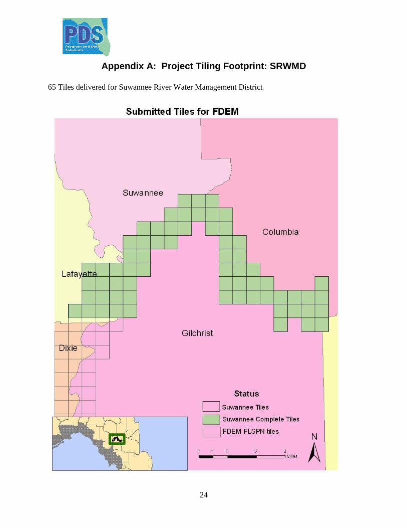
Appendix A: Project Tiling Footprint: SRWMD
65 Tiles delivered for Suwannee River Water Management District
25
List of delivered Tiles (65):
067291_N
067292_N
067293_N
067830_N
067831_N
067832_N
067833_N
067834_N
068368_N
068369_N
068370_N
068371_N
068373_N
068374_N
068907_N
068908_N
068909_N
068910_N
068914_N
068915_N
069447_N
069448_N
069454_N
069455_N
069984_N
069985_N
069986_N
069987_N
069988_N
069994_N
069995_N
069996_N
070524_N
070525_N
070526_N
070527_N
070534_N
070535_N
070536_N
070537_N
070541_N
072158_N
072160_N
072161_N
071064_N
071065_N
071066_N
071067_N
071074_N
071075_N
071076_N
071077_N
071078_N
071079_N
071080_N
071081_N
071607_N
071618_N
071619_N
071620_N
071621_N
071603_N
071604_N
071605_N
071606_N
26
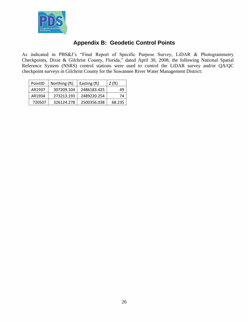
Appendix B: Geodetic Control Points
As indicated in PBS&J‟s “Final Report of Specific Purpose Survey, LiDAR & Photogrammetry
Checkpoints, Dixie & Gilchrist County, Florida,” dated April 30, 2008, the following National Spatial
Reference System (NSRS) control stations were used to control the LiDAR survey and/or QA/QC
checkpoint surveys in Gilchrist County for the Suwannee River Water Management District:
PointID Northing (ft) Easting (ft) Z (ft)
AR1937 307209.104 2486183.425 49
AR1934 273213.193 2489220.254 74
720507 326124.278 2500356.038 68.235
27
Appendix C: Data Dictionary
28
Table of Contents Horizontal and Vertical Datum ................................................................................................................................................................. 29
Coordinate System and Projection ............................................................................................................................................................ 29
Contour Topology Rules ........................................................................................................................................................................... 29
Breakline Topology Rules ........................................................................................................................................................................ 30
Coastal Shoreline ...................................................................................................................................................................................... 26
Linear Hydrographic Features .................................................................................................................................................................. 33
Closed Water Body Features .................................................................................................................................................................... 35
Road Features............................................................................................................................................................................................ 37
Bridge and Overpass Features .................................................................................................................................................................. 38
Soft Features ............................................................................................................................................................................................. 39
Island Features .......................................................................................................................................................................................... 40
Low Confidence Areas ............................................................................................................................................................................. 42
Masspoint .................................................................................................................................................................................................. 43
1 Foot Contours......................................................................................................................................................................................... 44
2 Foot Contours......................................................................................................................................................................................... 46
Ground Control ......................................................................................................................................................................................... 48
Vertical Accuracy Test Points .................................................................................................................................................................. 49
Footprint (Tile Boundaries) ...................................................................................................................................................................... 45
Contact Information .................................................................................................................................................................................. 45
29
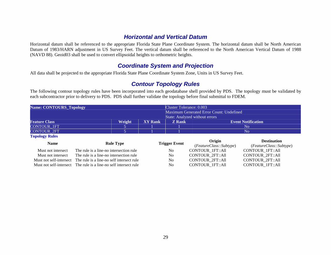
Horizontal and Vertical Datum Horizontal datum shall be referenced to the appropriate Florida State Plane Coordinate System. The horizontal datum shall be North American
Datum of 1983/HARN adjustment in US Survey Feet. The vertical datum shall be referenced to the North American Vertical Datum of 1988
(NAVD 88). Geoid03 shall be used to convert ellipsoidal heights to orthometric heights.
Coordinate System and Projection All data shall be projected to the appropriate Florida State Plane Coordinate System Zone, Units in US Survey Feet.
Contour Topology Rules The following contour topology rules have been incorporated into each geodatabase shell provided by PDS. The topology must be validated by
each subcontractor prior to delivery to PDS. PDS shall further validate the topology before final submittal to FDEM.
Name: CONTOURS_Topology Cluster Tolerance: 0.003
Maximum Generated Error Count: Undefined
State: Analyzed without errors
Feature Class Weight XY Rank Z Rank Event Notification CONTOUR_1FT 5 1 1 No
CONTOUR_2FT 5 1 1 No
Topology Rules
Name Rule Type Trigger Event Origin
(FeatureClass::Subtype) Destination
(FeatureClass::Subtype)
Must not intersect The rule is a line-no intersection rule No CONTOUR_1FT::All CONTOUR_1FT::All
Must not intersect The rule is a line-no intersection rule No CONTOUR_2FT::All CONTOUR_2FT::All
Must not self-intersect The rule is a line-no self intersect rule No CONTOUR_2FT::All CONTOUR_2FT::All
Must not self-intersect The rule is a line-no self intersect rule No CONTOUR_1FT::All CONTOUR_1FT::All
30
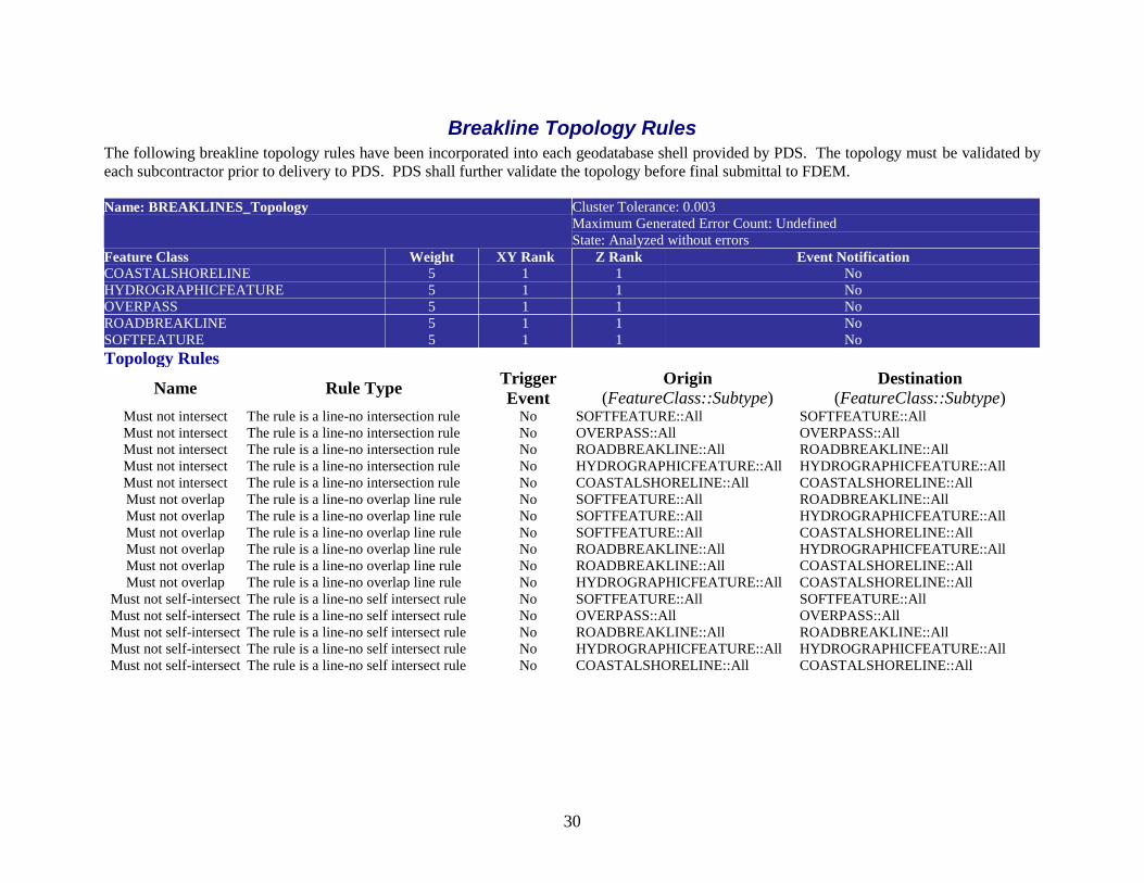
Breakline Topology Rules The following breakline topology rules have been incorporated into each geodatabase shell provided by PDS. The topology must be validated by
each subcontractor prior to delivery to PDS. PDS shall further validate the topology before final submittal to FDEM.
Name: BREAKLINES_Topology Cluster Tolerance: 0.003
Maximum Generated Error Count: Undefined
State: Analyzed without errors
Feature Class Weight XY Rank Z Rank Event Notification COASTALSHORELINE 5 1 1 No
HYDROGRAPHICFEATURE 5 1 1 No
OVERPASS 5 1 1 No
ROADBREAKLINE 5 1 1 No
SOFTFEATURE 5 1 1 No
Topology Rules
Name Rule Type Trigger
Event
Origin (FeatureClass::Subtype)
Destination (FeatureClass::Subtype)
Must not intersect The rule is a line-no intersection rule No SOFTFEATURE::All SOFTFEATURE::All
Must not intersect The rule is a line-no intersection rule No OVERPASS::All OVERPASS::All
Must not intersect The rule is a line-no intersection rule No ROADBREAKLINE::All ROADBREAKLINE::All
Must not intersect The rule is a line-no intersection rule No HYDROGRAPHICFEATURE::All HYDROGRAPHICFEATURE::All
Must not intersect The rule is a line-no intersection rule No COASTALSHORELINE::All COASTALSHORELINE::All
Must not overlap The rule is a line-no overlap line rule No SOFTFEATURE::All ROADBREAKLINE::All
Must not overlap The rule is a line-no overlap line rule No SOFTFEATURE::All HYDROGRAPHICFEATURE::All
Must not overlap The rule is a line-no overlap line rule No SOFTFEATURE::All COASTALSHORELINE::All
Must not overlap The rule is a line-no overlap line rule No ROADBREAKLINE::All HYDROGRAPHICFEATURE::All
Must not overlap The rule is a line-no overlap line rule No ROADBREAKLINE::All COASTALSHORELINE::All
Must not overlap The rule is a line-no overlap line rule No HYDROGRAPHICFEATURE::All COASTALSHORELINE::All
Must not self-intersect The rule is a line-no self intersect rule No SOFTFEATURE::All SOFTFEATURE::All
Must not self-intersect The rule is a line-no self intersect rule No OVERPASS::All OVERPASS::All
Must not self-intersect The rule is a line-no self intersect rule No ROADBREAKLINE::All ROADBREAKLINE::All
Must not self-intersect The rule is a line-no self intersect rule No HYDROGRAPHICFEATURE::All HYDROGRAPHICFEATURE::All
Must not self-intersect The rule is a line-no self intersect rule No COASTALSHORELINE::All COASTALSHORELINE::All
31
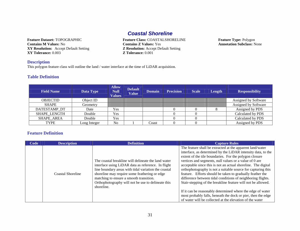
Coastal Shoreline Feature Dataset: TOPOGRAPHIC Feature Class: COASTALSHORELINE Feature Type: Polygon
Contains M Values: No Contains Z Values: Yes Annotation Subclass: None
XY Resolution: Accept Default Setting Z Resolution: Accept Default Setting
XY Tolerance: 0.003 Z Tolerance: 0.001
Description This polygon feature class will outline the land / water interface at the time of LiDAR acquisition.
Table Definition
Field Name Data Type
Allow
Null
Values
Default
Value Domain Precision Scale Length
Responsibility
OBJECTID Object ID Assigned by Software
SHAPE Geometry Assigned by Software
DATESTAMP_DT Date Yes 0 0 8 Assigned by PDS
SHAPE_LENGTH Double Yes 0 0 Calculated by PDS
SHAPE_AREA Double Yes 0 0 Calculated by PDS
TYPE Long Integer No 1 Coast 0 0 Assigned by PDS
Feature Definition
Code Description Definition Capture Rules
Coastal Shoreline
The coastal breakline will delineate the land water
interface using LiDAR data as reference. In flight
line boundary areas with tidal variation the coastal
shoreline may require some feathering or edge
matching to ensure a smooth transition.
Orthophotography will not be use to delineate this
shoreline.
The feature shall be extracted at the apparent land/water
interface, as determined by the LiDAR intensity data, to the
extent of the tile boundaries. For the polygon closure
vertices and segments, null values or a value of 0 are
acceptable since this is not an actual shoreline. The digital
orthophotography is not a suitable source for capturing this
feature. Efforts should be taken to gradually feather the
difference between tidal conditions of neighboring flights.
Stair-stepping of the breakline feature will not be allowed.
If it can be reasonably determined where the edge of water
most probably falls, beneath the dock or pier, then the edge
of water will be collected at the elevation of the water
32
where it can be directly measured. If there is a clearly-
indicated headwall or bulkhead adjacent to the dock or pier
and it is evident that the waterline is most probably adjacent
to the headwall or bulkhead, then the water line will follow
the headwall or bulkhead at the elevation of the water
where it can be directly measured. If there is no clear
indication of the location of the water‟s edge beneath the
dock or pier, then the edge of water will follow the outer
edge of the dock or pier as it is adjacent to the water, at the
measured elevation of the water.
Breaklines shall snap and merge seamlessly with linear
hydrographic features.
33
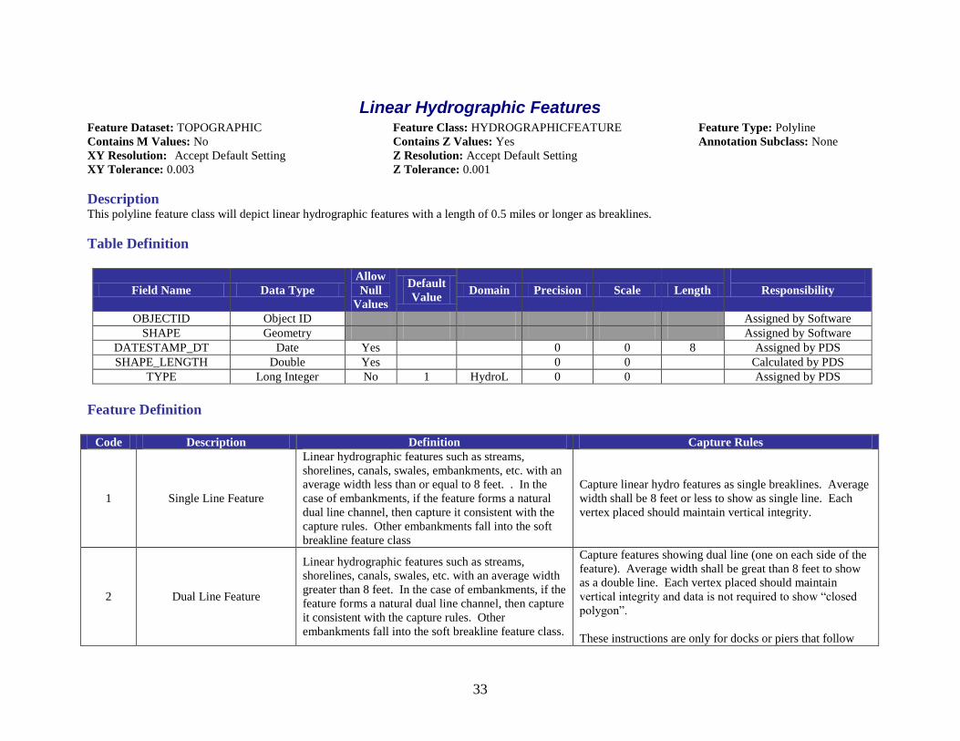
Linear Hydrographic Features Feature Dataset: TOPOGRAPHIC Feature Class: HYDROGRAPHICFEATURE Feature Type: Polyline
Contains M Values: No Contains Z Values: Yes Annotation Subclass: None
XY Resolution: Accept Default Setting Z Resolution: Accept Default Setting
XY Tolerance: 0.003 Z Tolerance: 0.001
Description This polyline feature class will depict linear hydrographic features with a length of 0.5 miles or longer as breaklines.
Table Definition
Field Name Data Type
Allow
Null
Values
Default
Value Domain Precision Scale Length
Responsibility
OBJECTID Object ID Assigned by Software
SHAPE Geometry Assigned by Software
DATESTAMP_DT Date Yes 0 0 8 Assigned by PDS
SHAPE_LENGTH Double Yes 0 0 Calculated by PDS
TYPE Long Integer No 1 HydroL 0 0 Assigned by PDS
Feature Definition
Code Description Definition Capture Rules
1 Single Line Feature
Linear hydrographic features such as streams,
shorelines, canals, swales, embankments, etc. with an
average width less than or equal to 8 feet. . In the
case of embankments, if the feature forms a natural
dual line channel, then capture it consistent with the
capture rules. Other embankments fall into the soft
breakline feature class
Capture linear hydro features as single breaklines. Average
width shall be 8 feet or less to show as single line. Each
vertex placed should maintain vertical integrity.
2 Dual Line Feature
Linear hydrographic features such as streams,
shorelines, canals, swales, etc. with an average width
greater than 8 feet. In the case of embankments, if the
feature forms a natural dual line channel, then capture
it consistent with the capture rules. Other
embankments fall into the soft breakline feature class.
Capture features showing dual line (one on each side of the
feature). Average width shall be great than 8 feet to show
as a double line. Each vertex placed should maintain
vertical integrity and data is not required to show “closed
polygon”.
These instructions are only for docks or piers that follow
34
the coastline or water‟s edge, not for docks or piers that
extend perpendicular from the land into the water. If it can
be reasonably determined where the edge of water most
probably falls, beneath the dock or pier, then the edge of
water will be collected at the elevation of the water where it
can be directly measured. If there is a clearly-indicated
headwall or bulkhead adjacent to the dock or pier and it is
evident that the waterline is most probably adjacent to the
headwall or bulkhead, then the water line will follow the
headwall or bulkhead at the elevation of the water where it
can be directly measured. If there is no clear indication of
the location of the water‟s edge beneath the dock or pier,
then the edge of water will follow the outer edge of the
dock or pier as it is adjacent to the water, at the measured
elevation of the water.
3 Soft Hydro Single Line
Feature
Linear hydro features with an average width less than
8 feet that compilation staff originally coded as soft
features due to unclear definition of hydro feature, but
that have been determined to be hydro features by
FDEM. Connectivity and monotonicity are not
enforced on these features.
Capture linear hydro features as single breaklines. Average
width shall be 8 feet or less to show as single line.
4 Soft Hydro Dual Line Feature
Linear hydro features with an average width greater
than 8 feet that compilation staff originally coded as
soft features due to unclear definition of hydro
feature, but that have been determined to be hydro
features by FDEM. Connectivity and monotonicity
are not enforced on these features.
Capture features showing dual line (one on each side of the
feature). Average width shall be greater than 8 feet to show
as a double line. Data is not required to show “closed
polygon”.
Note: Carry through bridges for all linear hydrographic features.
35
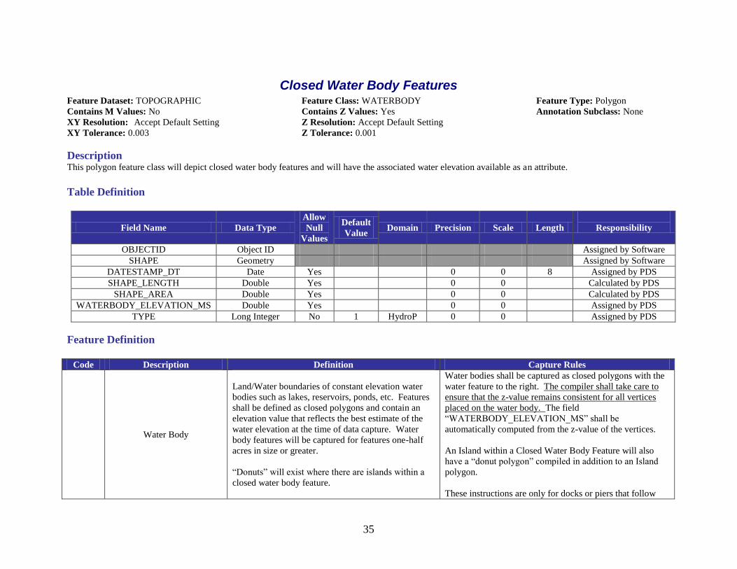
Closed Water Body Features Feature Dataset: TOPOGRAPHIC Feature Class: WATERBODY Feature Type: Polygon
Contains M Values: No Contains Z Values: Yes Annotation Subclass: None
XY Resolution: Accept Default Setting Z Resolution: Accept Default Setting
XY Tolerance: 0.003 Z Tolerance: 0.001
Description This polygon feature class will depict closed water body features and will have the associated water elevation available as an attribute.
Table Definition
Field Name Data Type
Allow
Null
Values
Default
Value Domain Precision Scale Length
Responsibility
OBJECTID Object ID Assigned by Software
SHAPE Geometry Assigned by Software
DATESTAMP_DT Date Yes 0 0 8 Assigned by PDS
SHAPE_LENGTH Double Yes 0 0 Calculated by PDS
SHAPE_AREA Double Yes 0 0 Calculated by PDS
WATERBODY_ELEVATION_MS Double Yes 0 0 Assigned by PDS
TYPE Long Integer No 1 HydroP 0 0 Assigned by PDS
Feature Definition
Code Description Definition Capture Rules
Water Body
Land/Water boundaries of constant elevation water
bodies such as lakes, reservoirs, ponds, etc. Features
shall be defined as closed polygons and contain an
elevation value that reflects the best estimate of the
water elevation at the time of data capture. Water
body features will be captured for features one-half
acres in size or greater.
“Donuts” will exist where there are islands within a
closed water body feature.
Water bodies shall be captured as closed polygons with the
water feature to the right. The compiler shall take care to
ensure that the z-value remains consistent for all vertices
placed on the water body. The field
“WATERBODY_ELEVATION_MS” shall be
automatically computed from the z-value of the vertices.
An Island within a Closed Water Body Feature will also
have a “donut polygon” compiled in addition to an Island
polygon.
These instructions are only for docks or piers that follow
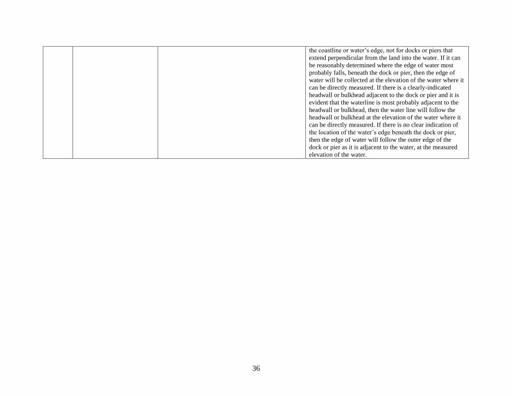
36
the coastline or water‟s edge, not for docks or piers that
extend perpendicular from the land into the water. If it can
be reasonably determined where the edge of water most
probably falls, beneath the dock or pier, then the edge of
water will be collected at the elevation of the water where it
can be directly measured. If there is a clearly-indicated
headwall or bulkhead adjacent to the dock or pier and it is
evident that the waterline is most probably adjacent to the
headwall or bulkhead, then the water line will follow the
headwall or bulkhead at the elevation of the water where it
can be directly measured. If there is no clear indication of
the location of the water‟s edge beneath the dock or pier,
then the edge of water will follow the outer edge of the
dock or pier as it is adjacent to the water, at the measured
elevation of the water.
37
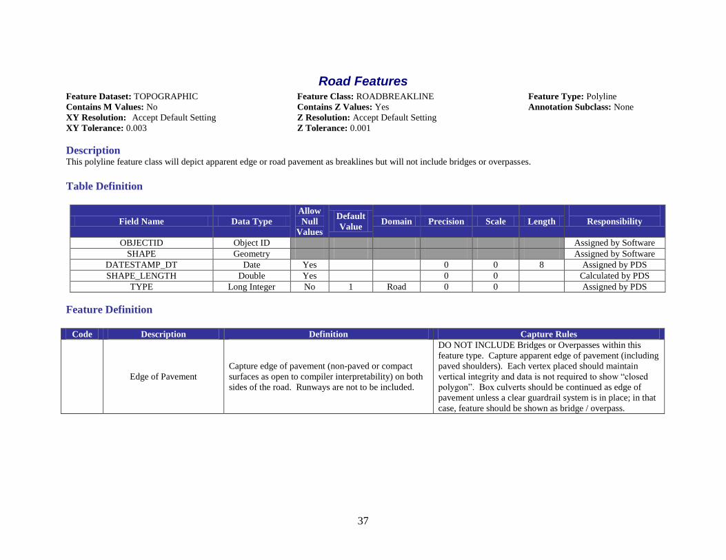
Road Features Feature Dataset: TOPOGRAPHIC Feature Class: ROADBREAKLINE Feature Type: Polyline
Contains M Values: No Contains Z Values: Yes Annotation Subclass: None
XY Resolution: Accept Default Setting Z Resolution: Accept Default Setting
XY Tolerance: 0.003 Z Tolerance: 0.001
Description This polyline feature class will depict apparent edge or road pavement as breaklines but will not include bridges or overpasses.
Table Definition
Field Name Data Type
Allow
Null
Values
Default
Value Domain Precision Scale Length
Responsibility
OBJECTID Object ID Assigned by Software
SHAPE Geometry Assigned by Software
DATESTAMP_DT Date Yes 0 0 8 Assigned by PDS
SHAPE_LENGTH Double Yes 0 0 Calculated by PDS
TYPE Long Integer No 1 Road 0 0 Assigned by PDS
Feature Definition
Code Description Definition Capture Rules
Edge of Pavement
Capture edge of pavement (non-paved or compact
surfaces as open to compiler interpretability) on both
sides of the road. Runways are not to be included.
DO NOT INCLUDE Bridges or Overpasses within this
feature type. Capture apparent edge of pavement (including
paved shoulders). Each vertex placed should maintain
vertical integrity and data is not required to show “closed
polygon”. Box culverts should be continued as edge of
pavement unless a clear guardrail system is in place; in that
case, feature should be shown as bridge / overpass.
38
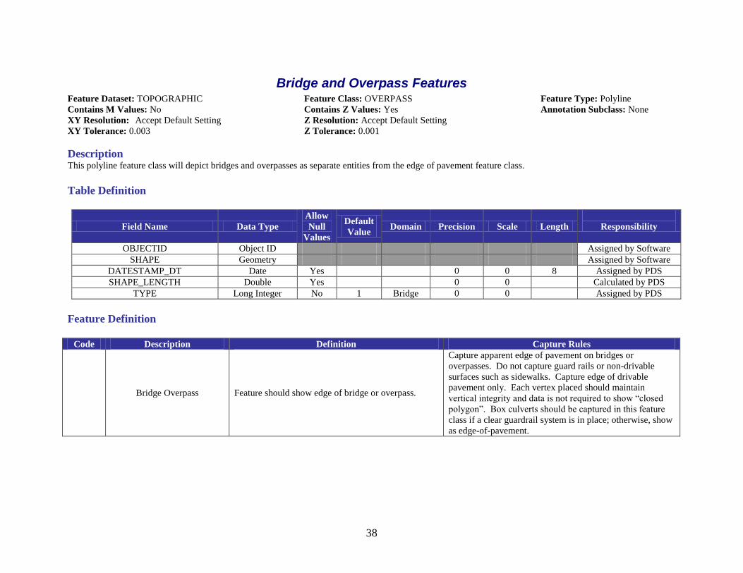
Bridge and Overpass Features Feature Dataset: TOPOGRAPHIC Feature Class: OVERPASS Feature Type: Polyline
Contains M Values: No Contains Z Values: Yes Annotation Subclass: None
XY Resolution: Accept Default Setting Z Resolution: Accept Default Setting
XY Tolerance: 0.003 Z Tolerance: 0.001
Description This polyline feature class will depict bridges and overpasses as separate entities from the edge of pavement feature class.
Table Definition
Field Name Data Type
Allow
Null
Values
Default
Value Domain Precision Scale Length
Responsibility
OBJECTID Object ID Assigned by Software
SHAPE Geometry Assigned by Software
DATESTAMP_DT Date Yes 0 0 8 Assigned by PDS
SHAPE_LENGTH Double Yes 0 0 Calculated by PDS
TYPE Long Integer No 1 Bridge 0 0 Assigned by PDS
Feature Definition
Code Description Definition Capture Rules
Bridge Overpass Feature should show edge of bridge or overpass.
Capture apparent edge of pavement on bridges or
overpasses. Do not capture guard rails or non-drivable
surfaces such as sidewalks. Capture edge of drivable
pavement only. Each vertex placed should maintain
vertical integrity and data is not required to show “closed
polygon”. Box culverts should be captured in this feature
class if a clear guardrail system is in place; otherwise, show
as edge-of-pavement.
39
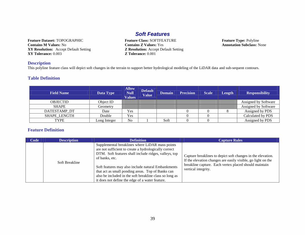
Soft Features Feature Dataset: TOPOGRAPHIC Feature Class: SOFTFEATURE Feature Type: Polyline
Contains M Values: No Contains Z Values: Yes Annotation Subclass: None
XY Resolution: Accept Default Setting Z Resolution: Accept Default Setting
XY Tolerance: 0.003 Z Tolerance: 0.001
Description This polyline feature class will depict soft changes in the terrain to support better hydrological modeling of the LiDAR data and sub-sequent contours.
Table Definition
Field Name Data Type
Allow
Null
Values
Default
Value Domain Precision Scale Length
Responsibility
OBJECTID Object ID Assigned by Software
SHAPE Geometry Assigned by Software
DATESTAMP_DT Date Yes 0 0 8 Assigned by PDS
SHAPE_LENGTH Double Yes 0 0 Calculated by PDS
TYPE Long Integer No 1 Soft 0 0 Assigned by PDS
Feature Definition
Code Description Definition Capture Rules
Soft Breakline
Supplemental breaklines where LiDAR mass points
are not sufficient to create a hydrologically correct
DTM. Soft features shall include ridges, valleys, top
of banks, etc.
Soft features may also include natural Embankments
that act as small ponding areas. Top of Banks can
also be included in the soft breakline class so long as
it does not define the edge of a water feature.
Capture breaklines to depict soft changes in the elevation.
If the elevation changes are easily visible, go light on the
breakline capture. Each vertex placed should maintain
vertical integrity.
40
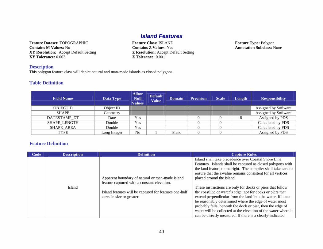
Island Features Feature Dataset: TOPOGRAPHIC Feature Class: ISLAND Feature Type: Polygon
Contains M Values: No Contains Z Values: Yes Annotation Subclass: None
XY Resolution: Accept Default Setting Z Resolution: Accept Default Setting
XY Tolerance: 0.003 Z Tolerance: 0.001
Description This polygon feature class will depict natural and man-made islands as closed polygons.
Table Definition
Field Name Data Type
Allow
Null
Values
Default
Value Domain Precision Scale Length
Responsibility
OBJECTID Object ID Assigned by Software
SHAPE Geometry Assigned by Software
DATESTAMP_DT Date Yes 0 0 8 Assigned by PDS
SHAPE_LENGTH Double Yes 0 0 Calculated by PDS
SHAPE_AREA Double Yes 0 0 Calculated by PDS
TYPE Long Integer No 1 Island 0 0 Assigned by PDS
Feature Definition
Code Description Definition Capture Rules
Island
Apparent boundary of natural or man-made island
feature captured with a constant elevation.
Island features will be captured for features one-half
acres in size or greater.
Island shall take precedence over Coastal Shore Line
Features. Islands shall be captured as closed polygons with
the land feature to the right. The compiler shall take care to
ensure that the z-value remains consistent for all vertices
placed around the island.
These instructions are only for docks or piers that follow
the coastline or water‟s edge, not for docks or piers that
extend perpendicular from the land into the water. If it can
be reasonably determined where the edge of water most
probably falls, beneath the dock or pier, then the edge of
water will be collected at the elevation of the water where it
can be directly measured. If there is a clearly-indicated
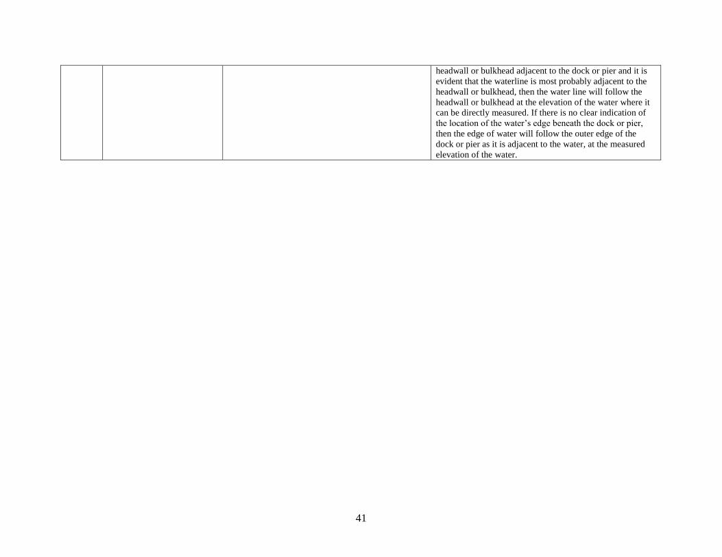
41
headwall or bulkhead adjacent to the dock or pier and it is
evident that the waterline is most probably adjacent to the
headwall or bulkhead, then the water line will follow the
headwall or bulkhead at the elevation of the water where it
can be directly measured. If there is no clear indication of
the location of the water‟s edge beneath the dock or pier,
then the edge of water will follow the outer edge of the
dock or pier as it is adjacent to the water, at the measured
elevation of the water.
42
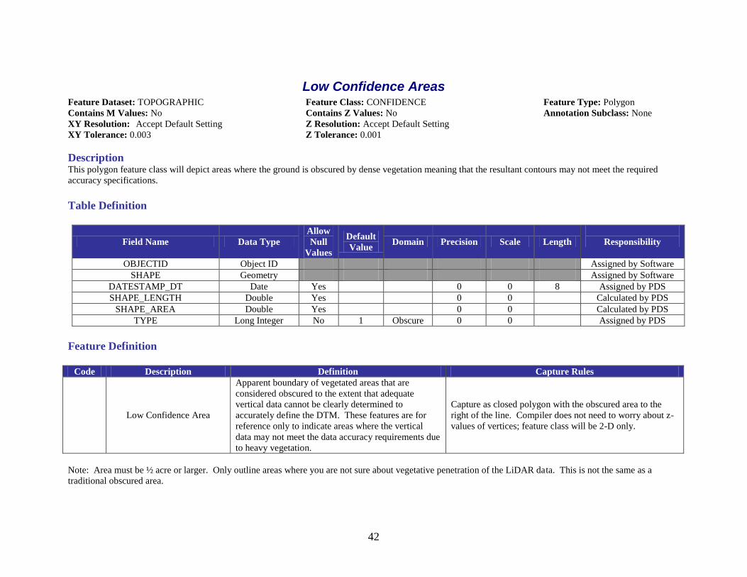
Low Confidence Areas Feature Dataset: TOPOGRAPHIC Feature Class: CONFIDENCE Feature Type: Polygon
Contains M Values: No Contains Z Values: No Annotation Subclass: None
XY Resolution: Accept Default Setting Z Resolution: Accept Default Setting
XY Tolerance: 0.003 Z Tolerance: 0.001
Description This polygon feature class will depict areas where the ground is obscured by dense vegetation meaning that the resultant contours may not meet the required
accuracy specifications.
Table Definition
Field Name Data Type
Allow
Null
Values
Default
Value Domain Precision Scale Length
Responsibility
OBJECTID Object ID Assigned by Software
SHAPE Geometry Assigned by Software
DATESTAMP_DT Date Yes 0 0 8 Assigned by PDS
SHAPE_LENGTH Double Yes 0 0 Calculated by PDS
SHAPE_AREA Double Yes 0 0 Calculated by PDS
TYPE Long Integer No 1 Obscure 0 0 Assigned by PDS
Feature Definition
Code Description Definition Capture Rules
Low Confidence Area
Apparent boundary of vegetated areas that are
considered obscured to the extent that adequate
vertical data cannot be clearly determined to
accurately define the DTM. These features are for
reference only to indicate areas where the vertical
data may not meet the data accuracy requirements due
to heavy vegetation.
Capture as closed polygon with the obscured area to the
right of the line. Compiler does not need to worry about z-
values of vertices; feature class will be 2-D only.
Note: Area must be ½ acre or larger. Only outline areas where you are not sure about vegetative penetration of the LiDAR data. This is not the same as a
traditional obscured area.
43
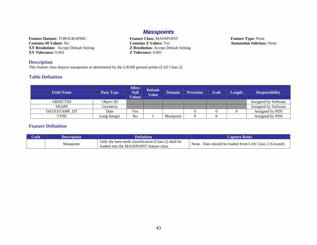
Masspoints Feature Dataset: TOPOGRAPHIC Feature Class: MASSPOINT Feature Type: Point
Contains M Values: No Contains Z Values: Yes Annotation Subclass: None
XY Resolution: Accept Default Setting Z Resolution: Accept Default Setting
XY Tolerance: 0.003 Z Tolerance: 0.001
Description This feature class depicts masspoints as determined by the LiDAR ground points (LAS Class 2).
Table Definition
Field Name Data Type
Allow
Null
Values
Default
Value Domain Precision Scale Length
Responsibility
OBJECTID Object ID Assigned by Software
SHAPE Geometry Assigned by Software
DATESTAMP_DT Date Yes 0 0 8 Assigned by PDS
TYPE Long Integer No 1 Masspoint 0 0 Assigned by PDS
Feature Definition
Code Description Definition Capture Rules
Masspoint Only the bare earth classification (Class 2) shall be
loaded into the MASSPOINT feature class. None. Data should be loaded from LAS Class 2 (Ground)
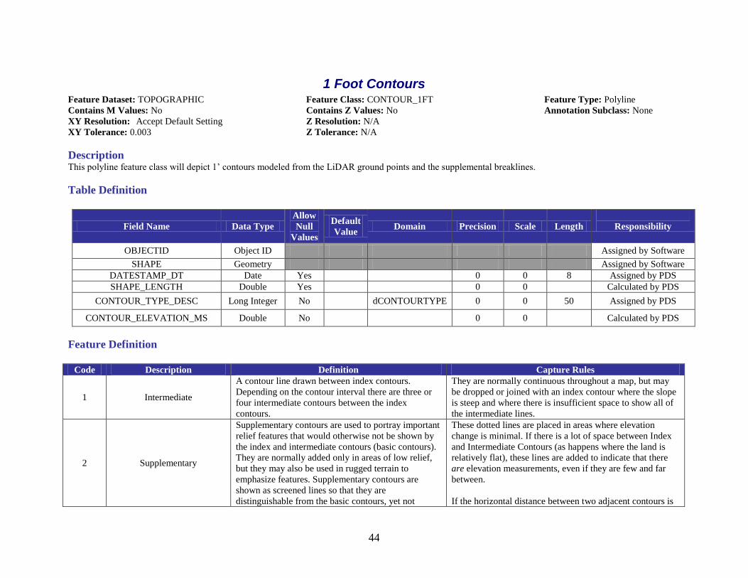
44
1 Foot Contours Feature Dataset: TOPOGRAPHIC Feature Class: CONTOUR_1FT Feature Type: Polyline
Contains M Values: No Contains Z Values: No Annotation Subclass: None
XY Resolution: Accept Default Setting Z Resolution: N/A
XY Tolerance: 0.003 Z Tolerance: N/A
Description This polyline feature class will depict 1‟ contours modeled from the LiDAR ground points and the supplemental breaklines.
Table Definition
Field Name Data Type
Allow
Null
Values
Default
Value Domain Precision Scale Length
Responsibility
OBJECTID Object ID Assigned by Software
SHAPE Geometry Assigned by Software
DATESTAMP_DT Date Yes 0 0 8 Assigned by PDS
SHAPE_LENGTH Double Yes 0 0 Calculated by PDS
CONTOUR_TYPE_DESC Long Integer No dCONTOURTYPE 0 0 50 Assigned by PDS
CONTOUR_ELEVATION_MS Double No 0 0 Calculated by PDS
Feature Definition
Code Description Definition Capture Rules
1 Intermediate
A contour line drawn between index contours.
Depending on the contour interval there are three or
four intermediate contours between the index
contours.
They are normally continuous throughout a map, but may
be dropped or joined with an index contour where the slope
is steep and where there is insufficient space to show all of
the intermediate lines.
2 Supplementary
Supplementary contours are used to portray important
relief features that would otherwise not be shown by
the index and intermediate contours (basic contours).
They are normally added only in areas of low relief,
but they may also be used in rugged terrain to
emphasize features. Supplementary contours are
shown as screened lines so that they are
distinguishable from the basic contours, yet not
These dotted lines are placed in areas where elevation
change is minimal. If there is a lot of space between Index
and Intermediate Contours (as happens where the land is
relatively flat), these lines are added to indicate that there
are elevation measurements, even if they are few and far
between.
If the horizontal distance between two adjacent contours is
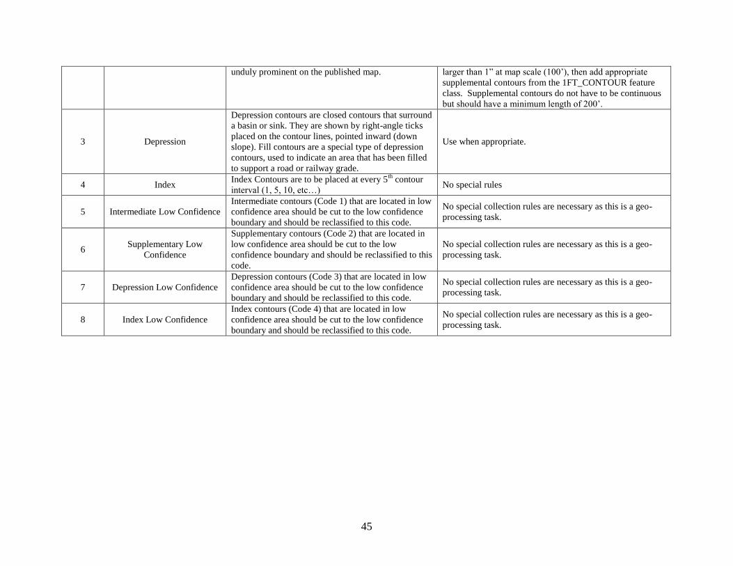
45
unduly prominent on the published map. larger than 1” at map scale (100‟), then add appropriate
supplemental contours from the 1FT_CONTOUR feature
class. Supplemental contours do not have to be continuous
but should have a minimum length of 200‟.
3 Depression
Depression contours are closed contours that surround
a basin or sink. They are shown by right-angle ticks
placed on the contour lines, pointed inward (down
slope). Fill contours are a special type of depression
contours, used to indicate an area that has been filled
to support a road or railway grade.
Use when appropriate.
4 Index Index Contours are to be placed at every 5
th contour
interval (1, 5, 10, etc…) No special rules
5 Intermediate Low Confidence
Intermediate contours (Code 1) that are located in low
confidence area should be cut to the low confidence
boundary and should be reclassified to this code.
No special collection rules are necessary as this is a geo-
processing task.
6 Supplementary Low
Confidence
Supplementary contours (Code 2) that are located in
low confidence area should be cut to the low
confidence boundary and should be reclassified to this
code.
No special collection rules are necessary as this is a geo-
processing task.
7 Depression Low Confidence
Depression contours (Code 3) that are located in low
confidence area should be cut to the low confidence
boundary and should be reclassified to this code.
No special collection rules are necessary as this is a geo-
processing task.
8 Index Low Confidence
Index contours (Code 4) that are located in low
confidence area should be cut to the low confidence
boundary and should be reclassified to this code.
No special collection rules are necessary as this is a geo-
processing task.
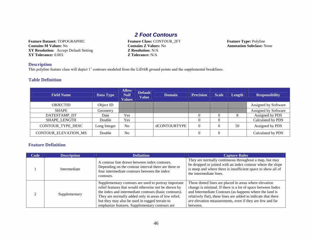
46
2 Foot Contours Feature Dataset: TOPOGRAPHIC Feature Class: CONTOUR_2FT Feature Type: Polyline
Contains M Values: No Contains Z Values: No Annotation Subclass: None
XY Resolution: Accept Default Setting Z Resolution: N/A
XY Tolerance: 0.003 Z Tolerance: N/A
Description This polyline feature class will depict 1‟ contours modeled from the LiDAR ground points and the supplemental breaklines.
Table Definition
Field Name Data Type
Allow
Null
Values
Default
Value Domain Precision Scale Length
Responsibility
OBJECTID Object ID Assigned by Software
SHAPE Geometry Assigned by Software
DATESTAMP_DT Date Yes 0 0 8 Assigned by PDS
SHAPE_LENGTH Double Yes 0 0 Calculated by PDS
CONTOUR_TYPE_DESC Long Integer No dCONTOURTYPE 0 0 50 Assigned by PDS
CONTOUR_ELEVATION_MS Double No 0 0 Calculated by PDS
Feature Definition
Code Description Definition Capture Rules
1 Intermediate
A contour line drawn between index contours.
Depending on the contour interval there are three or
four intermediate contours between the index
contours.
They are normally continuous throughout a map, but may
be dropped or joined with an index contour where the slope
is steep and where there is insufficient space to show all of
the intermediate lines.
2 Supplementary
Supplementary contours are used to portray important
relief features that would otherwise not be shown by
the index and intermediate contours (basic contours).
They are normally added only in areas of low relief,
but they may also be used in rugged terrain to
emphasize features. Supplementary contours are
These dotted lines are placed in areas where elevation
change is minimal. If there is a lot of space between Index
and Intermediate Contours (as happens where the land is
relatively flat), these lines are added to indicate that there
are elevation measurements, even if they are few and far
between.
47
shown as screened lines so that they are
distinguishable from the basic contours, yet not
unduly prominent on the published map.
If the horizontal distance between two adjacent contours is
larger than 1” at map scale (100‟), then add appropriate
supplemental contours from the 1FT_CONTOUR feature
class. Supplemental contours do not have to be continuous
but should have a minimum length of 200‟.
3 Depression
Depression contours are closed contours that surround
a basin or sink. They are shown by right-angle ticks
placed on the contour lines, pointed inward (down
slope). Fill contours are a special type of depression
contours, used to indicate an area that has been filled
to support a road or railway grade.
Use when appropriate.
4 Index Index Contours are to be placed at every 5
th contour
interval (1, 5, 10, etc…) No special rules
5 Intermediate Low Confidence
Intermediate contours (Code 1) that are located in low
confidence area should be cut to the low confidence
boundary and should be reclassified to this code.
No special collection rules are necessary as this is a geo-
processing task.
6 Supplementary Low
Confidence
Supplementary contours (Code 2) that are located in
low confidence area should be cut to the low
confidence boundary and should be reclassified to this
code.
No special collection rules are necessary as this is a geo-
processing task.
7 Depression Low Confidence
Depression contours (Code 3) that are located in low
confidence area should be cut to the low confidence
boundary and should be reclassified to this code.
No special collection rules are necessary as this is a geo-
processing task.
8 Index Low Confidence
Index contours (Code 4) that are located in low
confidence area should be cut to the low confidence
boundary and should be reclassified to this code.
No special collection rules are necessary as this is a geo-
processing task.
48
Ground Control Feature Dataset: TOPOGRAPHIC Feature Class: GROUNDCONTROL Feature Type: Point
Contains M Values: No Contains Z Values: Yes Annotation Subclass: None
XY Resolution: Accept Default Setting Z Resolution: Accept Default Setting
XY Tolerance: 0.003 Z Tolerance: 0.001
Description This feature class depicts the points used in the acquisition and calibration of the LiDAR and aerial photography collected by Aero-Metric, Sanborn and
Terrapoint.
Table Definition
Field Name Data Type
Allow
Null
Values
Default
Value Domain Precision Scale Length
Responsibility
OBJECTID Object ID Assigned by Software
SHAPE Geometry Assigned by Software
DATESTAMP_DT Date Yes 0 0 8 Assigned by PDS
TYPE Long Integer No 1 Control 0 0 Assigned by PDS
POINTID String Yes 12 Assigned by PDS
X_COORD Double Yes 0 0 Assigned by PDS
Y_COORD Double Yes 0 0 Assigned by PDS
Z_COORD Double Yes 0 0 Assigned by PDS
Feature Definition
Code Description Definition Capture Rules
Control Point
Primary or Secondary PDS control points used for
either base station operations or in the calibration and
adjustment of the control.
None.
49
Vertical Accuracy Test Points Feature Dataset: TOPOGRAPHIC Feature Class: VERTACCTESTPTS Feature Type: Point
Contains M Values: No Contains Z Values: Yes Annotation Subclass: None
XY Resolution: Accept Default Setting Z Resolution: Accept Default Setting
XY Tolerance: 0.003 Z Tolerance: 0.001
Description This feature class depicts the points used by PDS to test the vertical accuracy of the data produced.
Table Definition
Field Name Data Type
Allow
Null
Values
Default
Value Domain Precision Scale Length
Responsibility
OBJECTID Object ID Assigned by Software
SHAPE Geometry Assigned by Software
DATESTAMP_DT Date Yes 0 0 8 Assigned by PDS
POINTID String Yes 12 Assigned by PDS
X_COORD Double Yes 0 0 Assigned by PDS
Y_COORD Double Yes 0 0 Assigned by PDS
Z_COORD Double Yes 0 0 Assigned by PDS
LANDCOVER Long Integer No 1 dLANDCOVERTYPE 0 0 Assigned by PDS
Feature Definition
Code Description Definition Capture Rules
1 Bare-Earth and Low Grass None. None.
2 Brush Lands and Low Trees None. None.
3 Forested Areas Fully Covered
by Trees None. None.
4 Urban Areas None. None.
50
Footprint (Tile Boundaries) Feature Dataset: TOPOGRAPHIC Feature Class: FOOTPRINT Feature Type: Polygon
Contains M Values: No Contains Z Values: No Annotation Subclass: None
XY Resolution: Accept Default Setting Z Resolution: Accept Default Setting
XY Tolerance: 0.003 Z Tolerance: 0.001
Description This polygon feature class includes the Florida 5,000‟ x 5,000‟ tiles for each countywide geodatabase produced.
Table Definition
Field Name Data Type
Allow
Null
Values
Default
Value Domain Precision Scale Length
Responsibility
OBJECTID Object ID Assigned by Software
SHAPE Geometry Assigned by Software
DATESTAMP_DT Date Yes 0 0 8 Assigned by PDS
SHAPE_LENGTH Double Yes 0 0 Calculated by PDS
SHAPE_AREA Double Yes 0 0 Calculated by PDS
CELLNUM String No 0 0 8 Assigned by PDS
Contact Information Any questions regarding this document should be addressed to:
Brian Mayfield, C.P., GISP, G.L.S.
Associate / Sr. Project Manager
Dewberry
8401 Arlington Blvd.
Fairfax, VA 22031
(703) 849-0254 – voice
(703) 340-4141 – cell
Appendix D: LiDAR Processing Report
PROJECT REPORT
Terrapoint #: 2007-205-U
Dewberry #: 07-HS-34-14-00-22-469 Task Order 20070525-4927
Florida (Suwannee River) 2008 LiDAR Collection
Originally submitted: 2009-03-11
Revisions: 2009-03-11
Presented to:
Fairfax, Virginia
Submitted by:
Houston, Texas
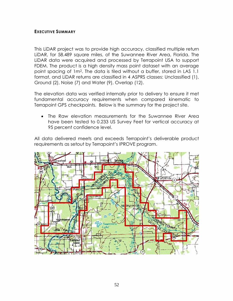
52
EXECUTIVE SUMMARY
This LiDAR project was to provide high accuracy, classified multiple return
LiDAR, for 58.489 square miles, of the Suwannee River Area, Florida. The
LiDAR data were acquired and processed by Terrapoint USA to support
FDEM. The product is a high density mass point dataset with an average
point spacing of 1m2. The data is tiled without a buffer, stored in LAS 1.1
format, and LiDAR returns are classified in 4 ASPRS classes: Unclassified (1),
Ground (2), Noise (7) and Water (9), Overlap (12).
The elevation data was verified internally prior to delivery to ensure it met
fundamental accuracy requirements when compared kinematic to
Terrapoint GPS checkpoints. Below is the summary for the project site.
The Raw elevation measurements for the Suwannee River Area
have been tested to 0.233 US Survey Feet for vertical accuracy at
95 percent confidence level.
All data delivered meets and exceeds Terrapoint’s deliverable product
requirements as setout by Terrapoint’s IPROVE program.
53
Project Report ...................................................................................................... 51
Executive Summary ............................................................................................. 52
Suwannee River Area Project Report ............................................................... 54
1 Introduction ................................................................................................... 54
2 Acquisition ..................................................................................................... 55
2.1 PARAMETER OVERVIEW ............................................................................... 55
2.2 GPS RECEIVERS.......................................................................................... 55
2.3 MISSIONS STATISTICS .................................................................................... 55
2.4 REFERENCE COORDINATE SYSTEM USED ........................................................ 56
2.4.1 Suwannee River ….………………………………………………............6
2.5 GEOID MODEL USED .................................................................................... 6
3 Processing ........................................................................................................ 7
3.1 AIRBORNE GPS KINEMATIC ........................................................................... 7
3.2 GENERATION AND CALIBRATION OF LASER POINTS (RAW DATA) ........................ 7
3.3 VERTICAL BIAS RESOLUTION ......................................................................... 60
3.4 DATA CLASSIFICATION AND EDITING ............................................................. 62
3.5 DELIVERABLE PRODUCT GENERATION ........................................................... 62
3.5.1 Deliverable Tiling Scheme .............................................................. 62
3.5.2 LiDAR Point Data ............................................................................. 62
3.5.3 FGDC Report ................................................................................... 63
4 Quality Control .............................................................................................. 63
4.1 QUALITY CONTROL FOR DATA ACQUISITION .................................................. 64
4.2 QUALITY CONTROL FOR DATA PROCESSING .................................................. 66
4.3 POSITIONAL ACCURACY .............................................................................. 68
4.3.1 Vertical Positional Accuracy ......................................................... 68
4.3.2 Horizontal Positional Accuracy ...................................................... 19
5 Conclusion ..................................................................................................... 70 Appendix A Suwannee River Area FGDC Metadata ..................................... 21
54
SUWANNEE RIVER AREA PROJECT REPORT
Introduction
LiDAR data is remotely sensed high-resolution elevation data collected by
an airborne collection platform. By positioning laser range finding with the
use of 1 second GPS with 200 Hz inertial measurement unit corrections;
Terrapoint's LiDAR instruments are able to make highly detailed geospatial
elevation products of the ground, man-made structures and vegetation.
The LiDAR ground extraction process takes place by building an iterative
surface model. This surface model is generated using three main
parameters: building size, iteration angle and iteration distance.
The purpose of this LiDAR data was to produce high accuracy 3D terrain
geospatial products for Suwannee River Area.
This report covers the mission parameter and details, processing step
outlines and deliverables.
This report is submitted as a supporting overview document for the FGDC
metadata reports that are included as an addendum to this report.
55
Acquisition
Parameter Overview
The Airborne LiDAR survey was conducted using one Optech 3100EA
system flying at a nominal height of 970 meters AGL with a total angular
coverage of 18.1 degrees with a 4 degree cutoff. Flight line spacing was
nominally 219.28 meters providing overlap of 55% on adjacent flight lines.
Lines were flown in east/west and north/south orientated blocks to best
optimize flying time considering the layout for the project. The aircraft was
a Navajo, registrations C-FQQB, used for the survey. This aircraft has a
flight range of approximately 6 hours and was flown at an average
altitude of 970 meters above sea level (ASL), thereby encountering flying
altitudes of approximately 970 meters above ground level (AGL). The
aircraft was staged from Gainesville Regional Airport (GNV), Gainesville,
Florida, and ferried daily to the project site for flight operations.
The Optech 3100EA system was configured in the following manner for the
Suwannee River Area:
Type of Scanner = Optech 3100EA
Data Acquisition Height = 970 meters AGL
Scanner Field of View = 18.1 degrees with a 4 degree cutoff
Scan Frequency = 55.2 Hertz
Pulse Repetition Rate = 100 Kilohertz
Aircraft Speed = 150 Knots
Swath Width = 487.29 m Nominal
Ground Sample Distance = 0.70 meters - no overlap
Number of Returns per Pulse = 4
Distance between Flight Lines = 219.28m
GPS Receivers
A combination of Sokkia GSR 2600 and NovAtel DL-4+ dual frequency GPS
receivers were used to support the airborne operations of this survey and
to establish the GPS control network.
Missions Statistics
56
For the Suwannee River Area, a total of 3 missions were flown for this
project with good meteorological and GPS conditions. 71 flight lines were
flown over the project site to provide complete coverage.
The LiDAR mission for the Suwannee River Area was carried out on January
25, 2008, and January 29, 2008.
Reference Coordinate System Used
Suwannee River Area
Two existing NGS (National Geodetic Survey) monument was observed in
a GPS control network.
Existing monument AR1937 and AR1934 were used as primary control for
this project.
The published horizontal datum of the NGS stations is NAD83 HARN and
the vertical datum NAVD88.
The following are the final coordinates of newly established control points
used in this project:
Station_ID: 720507
West_Longitude: -82 49 17.95219
North_Latitude: 29 53 09.58018
Ellips_Elev: -7.0903
Geoid Model Used
The Geoid03 geoid model, published by the NGS, was used to
transform all ellipsoidal heights to orthometric.
Processing
57
Airborne GPS Kinematic
Airborne GPS kinematic data was processed on-site using GrafNav
kinematic On-The-Fly (OTF) software. Flights were flown with a minimum of
6 satellites in view (130 above the horizon) and with a PDOP of better than
4.5. Distances from base station to aircraft were kept to a maximum of 30
km, to ensure a strong OTF (On-The-Fly) solution. For all flights, the GPS
data can be classified as excellent, with GPS residuals of 5cm average
but no larger than 9 cm being recorded.
Generation and Calibration of Laser Points (raw data)
Calibration is performed to eliminate systematic bias in the system, which
would result in a bias in the data. By determining the bias they can then
be modeled and the effects removed from the data. The manufacturer
initially calibrates the system on manufacture. Subsequently each mission
is checked and calibrated to ensure data quality.
Manufacturer Calibration
Manufacturer calibration was completed upon manufacture and upon
delivery of the system to Terrapoint. The manufacturer maintains and
calibrates each LiDAR system annually and upon any field visits to service
the system.
Manufacturer calibration addresses both radiometric and geometric
calibration. Radiometric calibration is to ensure that the laser meets
specification for pulse energy, width, and rise time, frequency and beam
divergence. These values are tested by the manufacturer and annually
certified. Radiometric calibration also checks the alignment between
transmitter and receiver and assures that alignment is optimal.
Geometric calibration is also conducted by the manufacturer both in the
laboratory and with onsite flights in previously surveyed areas. Range
calibration determines the first/last range offsets. Scanner calibration
provides values for scanner offset and scale. Position orientation
alignment provides Pos misalignment angles.
The Following are the manufacturer derived calibration values that are
constant unless the IMU is changed:
AltmSerialNo= 05Sen183
ImuType= LN200A1
ImuRate= 200
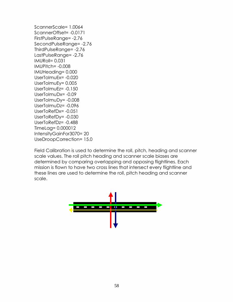
58
ScannerScale= 1.0064
ScannerOffset= -0.0171
FirstPulseRange= -2.76
SecondPulseRange= -2.76
ThirdPulseRange= -2.76
LastPulseRange= -2.76
IMURoll= 0.031
IMUPitch= -0.008
IMUHeading= 0.000
UserToImuEx= -0.020
UserToImuEy= 0.005
UserToImuEz= -0.150
UserToImuDx= -0.09
UserToImuDy= -0.008
UserToImuDz= -0.096
UserToRefDx= -0.051
UserToRefDy= -0.030
UserToRefDz= -0.488
TimeLag= 0.000012
IntensityGainFor3070= 20
UseDroopCorrection= 15.0
Field Calibration is used to determine the roll, pitch, heading and scanner
scale values. The roll pitch heading and scanner scale biases are
determined by comparing overlapping and opposing flightlines. Each
mission is flown to have two cross lines that intersect every flightline and
these lines are used to determine the roll, pitch heading and scanner
scale.
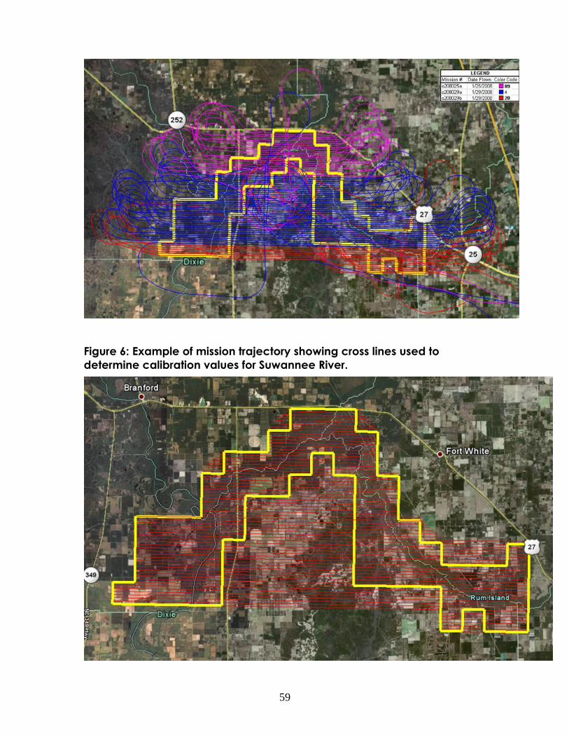
59
Figure 6: Example of mission trajectory showing cross lines used to
determine calibration values for Suwannee River.
60
Figure 2: Example of mission flight lines showing coverage of project area.
The mission data is initially output using the manufacturer calibration
default values for the specific system. The data is then examined using a
combination of Terrascan Terramodel and Terramatch and user input to
determine the final roll, pitch, and heading and scanner scale. Once the
values are finalized the mission data is output in LAS format.
The data is then checked against kinematic control data to ensure
vertical accuracy. Each mission’s data is based on the post-processed
position of a base station. The base stations used were all tied into
geodetic control points or were geodetic control points. Units are in US
Survey Feet.
Because of this, the positional accuracy of the LiDAR data is ensured. The
individual mission data can then be compared to adjoining missions to
ensure both vertical and horizontal accuracy. If any offset either vertical
of horizontal is found then the mission is reprocessed and checked for
accuracy.
Vertical Bias Resolution
Due to limitations in the Optech Dashmap software, occasionally the Dz
must be adjusted, post calibration, manually in Terrascan, to ensure that
each missions ties to adjoining missions and GPS kinematic validation
Table 1: Kinematic Point Comparison
Average dz -0.160
Minimum dz 0.262
Maximum dz -0.656
Average magnitude 0.187
Root mean square 0.233
Std deviation 0.170

61
points. The Suwannee River Area data did not require any adjustments to
the Dz.
62
Data Classification and Editing
The data was processed using the software Terrascan, and following the
methodology described herein. The initial step is the setup of the Terrascan
project, which is done by importing the Dewberry provided tile boundary index
encompassing the entire project areas. The 3D laser point clouds, in binary
format, were imported into the Terrascan project and divided in 65 tiles for the
Suwannee River Area, in LAS 1.0 format. Once tiled, the laser points were
classified using a proprietary routine in Terrascan. This routine removes any
obvious outliers from the dataset following which the ground layer is extracted
from the point cloud. The ground extraction process encompassed in this
routine takes place by building an iterative surface model. This surface model is
generated using three main parameters: building size, iteration angle and
iteration distance. The initial model is based on low points being selected by a
"roaming window" with the assumption is that these are the ground points. The
size of this roaming window is determined by the building size parameter. The
low points are triangulated and the remaining points are evaluated and
subsequently added to the model if they meet the iteration angle and distance
constraints. This process is repeated until no additional points are added within
iteration. A second critical parameter is the maximum terrain angle constraint,
which determines the maximum terrain angle allowed within the classification
model. The data is then manually quality controlled with the use of hillshading,
cross-sections and profiles. Any points found to be of class vegetation, building
or error during the quality control process, are removed from the ground model
and placed on the appropriate layer. An integrity check is also performed
simultaneously to verify that ground features such as rock cuts, elevated roads
and crests are present. Once data has been cleaned and complete, it is then
by a supervisor via manual inspection and through the use of a hillshade
mosaic.
Deliverable Product Generation
Deliverable Tiling Scheme
All files were retiled in the provided tiling scheme with a total of 65 tiles for
Suwannee River Area.
LiDAR Point Data
63
The LiDAR point data was delivered in LAS 1.1 adhering to the following
ASPRS classification scheme:
Class 1 – Unclassified
Class 2 – Ground
Class 7 – Noise
Class 9 – Water
Class 12 - Overlap
Water body delineation was collected using hillshades and intensity images
generated from ground DEM and LiDAR.
The LAS files contain the following fields of information (Precision reported in
brackets):
Class (Integer)
GPS Week Time (0.0001 seconds)
Easting (0.01 meter)
Northing (0.01 meter)
Elevation (0.01 meter)
Echo Number (Integer 1 to 4)
Echo (Integer 1 to 4)
Intensity (8 Bit Integer)
Flightline (Integer)
Scan Angle (Integer Degree)
Please note that the LiDAR intensity is not calibrated or normalized. The intensity
value is meant to provide relative signal return strengths for features imaged by
the sensor.
Point data was clipped to the project boundary.
FGDC Report
Separate metadata FGDC reports were delivered for the Suwannee River Area.
The reports are included as an addendum to this report.
Quality Control
64
Quality Control for Data Acquisition
A daily calibration flight is key to the QC process since it helps identify any
systematic issues in data acquisition or failures on the part of the GPS, IMU or
other equipment that may not have been evident to the LiDAR operator during
the mission. The aircraft initially performs a figure-8 manoeuvre over the selected
calibration site to collect calibration data for use in post-processing. The
calibration site is ideally selected in a relatively open, tree-less area where
several large buildings are located. The buildings used for calibration are
surveyed using both GPS and conventional survey methods. A local network of
GPS points are established to provide a baseline for conventional traversing
around the perimeter of the buildings.
Ground truth validation is used to assess the data quality and consistency over
sample areas of the project. To facilitate a confident evaluation, existing survey
control is used to validate the LiDAR data. Published survey control, where the
orthometric height (elevation) has been determined by precise differential
levelling observation, is deemed to be suitable.
Ground truth validation points may be collected for each of the any terrain
categories that Dewberry requires to establish RMSE accuracies for the LIDAR
project. These points must be gathered in flat or uniformly sloped terrain (<20%
slope) away from surface features such as stream banks, bridges or
embankments. If collected, these points will be used during data processing to
test the RMSEz accuracy of the final LiDAR data products.
The LiDAR operator performs kinematic post-processing of the aircraft GPS data
in conjunction with the data collected at the Reference Station in closest
proximity to the area flown. Double difference phase processing of the GPS
data is used to achieve the greatest accuracy. The GPS position accuracy is
assessed by comparison of forward and reverse processing solutions and a
review of the computational statistics. Any data anomalies are identified and
the necessary corrective actions are implemented prior to the next mission.
The quality control of LIDAR data and data products has proven to be a key
concern by Dewberry. Many specifications detail how to measure the quality of
LiDAR data given RMSE statistical methods to a 95% confidence level. In order
to assure meeting all levels of QC concerns, Terrapoint has quality control and
assurance steps in both the data acquisition phase and the data processing
phase. Any acquired data sets that fail these checks are flagged for re-
acquisition.
QC Step 1 - The Data Acquisition (DAQ) software performs automatic system
and subsystem tests on power-up to verify proper functionality of the entire data
65
acquisition system. Any anomalies are immediately investigated and corrected
by the LiDAR operator if possible. Any persistent problems are referred to the
engineering staff, which can usually resolve the issue by telephone and/or
email. In the unlikely event that these steps do not resolve the problem, a
trained engineer is immediately dispatched to the project site with the
appropriate test equipment and spare parts needed to repair the system.
QC Step 2 - The DAQ software continuously monitors the health and
performance of all subsystems. Any anomalies are recorded in the System Log
and reported to the LiDAR operator for resolution. If the operator is unable to
correct the problem, the engineering staffs are immediately notified. They
provide the operator with instructions or on-site assistance as needed to resolve
the problem.
The DAQ software also provides real-time terrain viewers that allow the operator
to directly monitor the data quality. Multiple returns from individual laser shots
are color coded to provide the operator with an indication of the degree of
penetration through dense vegetation. If any aspect of the data does not
appear to be acceptable, the operator will review system settings to determine
if an adjustment could improve the data quality. Navigation aids are provided
to alert both the pilot and operator to any line following errors that could
potentially compromise the data integrity. The pilot and operator review the
data and determine whether an immediate re-flight of the line is required.
QC Step 3 - After the mission is completed, raw LiDAR data on the removable
disk drive is transferred to the Field PC at the field operations staging area. An
automated QA/QC program scans the System Log as well as the raw data files
to detect potential errors. Any problems identified are reported to the operator
for further analysis. Data is also retrieved from all GPS Reference Stations, which
were active during the mission and transferred to the Field PC. The GPS data is
processed and tested for internal consistency and overall quality. Any errors or
limit violations are reported to the operator for more detailed evaluation.
QC Step 4 - The operators utilize a data viewer installed on the Field PC to
review selected portions of the acquired LiDAR data. This permits a more
thorough and detailed analysis than is possible in real-time during data
collection. Corrupted files or problems in the data itself are noted. If the data
indicates improper settings or operation of the LiDAR sensor, the operator
determines the appropriate corrective actions needed prior to the next mission.
QC Step 5 - All LiDAR and GPS data is copied from the Field PC onto Hard Drives:
one for transfer to data processing, and one for local backup. Each Hard drive
is reviewed to ensure data completeness and readability.
66
Quality Control for Data Processing
Quality assurance and quality control procedures for the raw LiDAR data and
processed deliverables for the DEM and DTM products are performed in an
iterative fashion through the entire data processing cycle. All final products pass
through a seven-step QC control check to verify that the data meets the criteria
specified by Dewberry.
Terrapoint has developed a rigorous and complete process, which does
everything possible to ensure data will meet or exceed the technical
specifications. Experience dealing with all ranges of difficulty in all types of
topographic regions has led to the development of our quality assurance
methods. Our goal is to confidently deliver a final product to Dewberry that is as
precise as possible, the first time. Terrapoint will go to extraordinary lengths to
make our customer completely satisfied. The following list provides a step-by-
step explanation of the process used by Terrapoint to review the data prior to
customer delivery.
QC Step 1 - Data collected by the LiDAR unit is reviewed for completeness and
to make sure all data is captured without errors or corrupted values. In addition,
all GPS, aircraft trajectory, mission information, and ground control files are
reviewed and logged into a database. At this time, the data will be confirmed
to have been acquired using instrumentation that records first and last returns
for each laser pulse, or multiple returns per laser pulse.
QC Step 2 - The LiDAR data is post processed and calibrated for as a preliminary
step for product delivery. At this time, the data are inspected for flight line
errors, flight line overlap, slivers or gaps in the data, point data minimums, or
issues with the LiDAR unit or GPS. Flight line swath overlap will be confirmed to
have adjacent flight lines at the tolerance specified by Dewberry for overlap
throughout the project area thus enabling an evaluation of data reproducibility
throughout the areas.
QC Step3 - The full-featured product is reviewed as a grid and as raw points and
attention is placed on locating and eliminating any outlier or anomalous points
beyond three-sigma values. These points may be spikes, unusually high points,
or pits, unusually low points. LiDAR points returning from low clouds, birds,
pollution, or noise in the system can cause spikes. Pit-like low returns can come
from water features or damp soils or from system noise. Either type of point
needs to be classified as an error point and eliminated from use by any grid
products. In addition to these outliers, the full-feature product is reviewed for
NO DATA points and regular looking non-surface errors like scan lines appearing
67
in the data. Also, steps between flight lines are measured and adjusted as
needed.
Unusual or odd-looking features and questionable returns are checked for
validity and compared against additional source material such as aerial photos,
USGS digital maps, local maps, or by field inspection. Most errors found at this
QC step can be resolved by re-calibration of the data set or by eliminating
specific problem points.
QC Step 4 - After the full-feature data is at a clean stage, all points are classified
as ground and unclassified features. Any non-regular structures or features like
radio towers, large rock outcrops, water bodies, bridges, piers, are confirmed to
be classified into the category specified by Dewberry for these feature types.
Additional data sets like commercially available data sources or data sources
provided by Dewberry may be used to assist and verify that points are assigned
into correct classifications.
QC Step 5 - After the full-featured data set is certified as passing for
completeness and for the removal of outliers, attention may be shifted to quality
controlling the bare-earth model. This product may take several iterations to
create it to the quality level that Dewberry is looking for. As both Terrapoint and
Dewberry inspect the bare-earth model, adjustments are made to fine-tune and
fix specific errors.
Adjustments to the bare-earth model are generally made to fix errors created
by over-mowing the data set along mountaintops, shorelines, or other areas of
high percent slope. Also, vegetation artefacts leave a signature surface that
appears bumpy or rough. Every effort is made to remove spurious vegetation
values and remnants from the bare-earth model. All adjustments are made by
re-classifying points from ground to unclassified or vice versa. No adjustments
are made to the final grid product, as other parties cannot easily reproduce
these types of adjustments from the original, raw data set.
QC Step 6 - Both RMSEz and RMSExy are inspected in the classified bare-earth
model and compared to project specifications. RMSEz is examined in open, flat
areas away from breaks and under specified vegetation categories. Neither
RMSEz nor RMSExy are compared to orthoimagery or existing building footprints.
Comparison against imagery can skew the determination of accuracy because
of the lean and shadows in the imagery.
Instead, a point to point comparison of a recently acquired or existing high
confidence ground survey point to its nearest neighbour LiDAR laser return point.
This is done in the raw data set and usually with Terrascan software. The
tolerance for finding a near-by LiDAR point elevation to compare to a survey
68
point elevation is that the two points must be within a 0.5m radius of each other
in open flat areas is made. If no LiDAR points can be found within in this
tolerance, then alternative methodologies are used to convert the LiDAR to a
TIN, though this can introduce biases and processing errors in the end products
and could cause the RMSE values to be skewed and fall beyond project
specifications.
QC Step 7 - A final QC step is made against all deliverables before they are sent
to Dewberry. The deliverables are checked for file naming convention, integrity
checks of the files, conformance to file format requirements, delivery media
readability, and file size limits. In addition, as data are delivered all requested
reports would be delivered as they become available.
Positional Accuracy
Vertical Positional Accuracy
The elevation data was verified internally prior to delivery to Dewberry to ensure
it met fundamental accuracy requirements when compared kinematic to
Terrapoint GPS checkpoints. Below is the summary for the project site.
The LiDAR dataset for Suwannee River Area was tested 0.071m vertical
accuracy at 95 percent confidence level, based on consolidated RMSEz
(0.035m) x 1.9600.
Horizontal Positional Accuracy
Compiled to meet 1 meter horizontal accuracy at the 95 percent
confidence level.
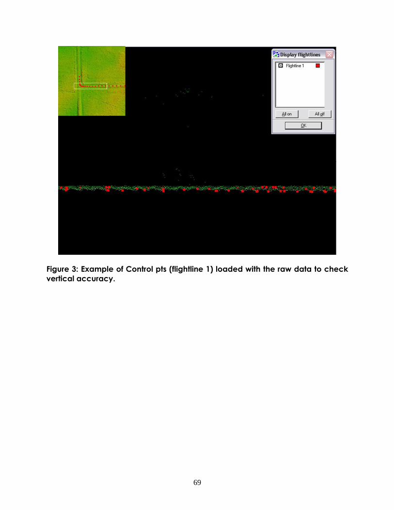
69
Figure 3: Example of Control pts (flightline 1) loaded with the raw data to check
vertical accuracy.

70
Conclusion
Overall the LiDAR data products submitted to Dewberry meet and exceed both
the absolute and relative accuracy requirements set out in the task order for this
project. The quality control requirements required in Terrapoint’s IPROVE
program were adhered to throughout the project cycle to ensure product
quality.
IDENTIFICATION_INFORMATION
71
Citation:
Citation_Information:
Originator: Terrapoint USA
Publication_Date: 20090311
Title: Dewberry FDEM Suwannee River Task Order 20070525-4927 Contract No. 07-HS-
34-14-00-22-469
Geospatial_Data_Presentation_Form: Map
Online_Linkage: none
Larger_Work_Citation:
Citation_Information:
Originator: Terrapoint USA
Publication_Date: 20090311
Title: Dewberry Dewberry FDEM Suwannee River Contract No. 2007-205-U
Publication_Information:
Publication_Place: Houston, Texas
Publisher: Terrapoint USA
Online_Linkage: none
Description:
Abstract:
LIDAR data is remotely sensed high-resolution elevation
data collected by an airborne collection platform. By
positioning laser range finding with the use of 1 second
GPS with 100hz inertial measurement unit corrections;
Terrapoint's LIDAR instruments are able to make highly
detailed geospatial elevation products of the ground,
man-made structures and vegetation. The
LiDAR flightlines for this project was planned for a 55%
acquisition overlap. The nominal resolution of this project
without overlap is 1.25m. Four returns were recorded for
each pulse in addition to an intensity value. GPS Week
Time, Intensity, Flightline and number attributes were
provided for each LiDAR point.
Data is provided as random points, in LAS v1.1 format,
classified in following code list 1=Unclassified 2=Ground
7=Noise 9=Water 12=Overlap
Purpose:
The purpose of this LiDAR data was to produce high accuracy
3D elevation based geospatial products for mapping.
Supplemental_Information:
LiDAR Collection Specific Supplemental Information:
- General Overview:
The Airborne LiDAR survey was conducted using 1 OPTECH
3100EA system flying at a nominal height of 970m AGL
72
with a total angular coverage of 20 degrees. Flight line spacing
was nominally 219.28m providing overlap of 55% on
adjacent flight lines. Lines were flown in east/west orientated blocks to best optimize flying
time
considering the layout for the project.
The total project size is 151.51 square kilometers
The aircraft was a PA-31 Navajos, registration C-FQQB,used for the survey. This aircraft has
a flight range of
approximately 6 hours and was flown at an average altitude
of 970 meters above sea level (ASL). The aircraft was staged from the
Gainesville Regional Airport, GNV, Gainesville, Florida, and ferried daily to
the project site for flight operations.
Aircraft Speed = 150 Knots
Number of Scanners = 1
Swath Width 451.45m Nominal
Distance Between Flight Lines = 225.72m
Data Acquisition Height = 970 meters AGL
Pulse Repetition Rate = 100 kHz
Number of Returns Per Pulse = 4
Scanner Field Of View = +/- 20 degrees
Scan Frequency = 55.2 Hertz
- GPS Receivers
A combination of Sokkia GSR 2600 and NovAtel DL-4+ dual
frequency GPS receivers were used to support the airborne
operations of this survey and to establish the GPS control
network.
- Number of Flights and Flight Lines
A total of 3 missions and 71 flightlines were flown for this project with flight
times ranging approximately 6 hours under good meteorological
and GPS conditions.
- Reference Coordinate System Used:
Existing monuments at AR1937 and AR1934 were used to control all flight missions and
kinematic ground surveys.
The published horizontal datum of the NGS stations is NAD83 HARN and the vertical datum
NAVD88. The following are the final coordinates of the new control used in this project:
Station_ID: 720507
West_Longitude: -82 49 17.95219
North_Latitude: 29 53 09.58018
Ellips_Elev: -7.0903
73
- Geoid Model Used
The Geoid03 geoid model, published by the NGS, was used to transform all
ellipsoidal heights to orthometric.
-General LiDAR notes
-Intensity
Please note that the LiDAR intensity is not calibrated or
normalized. The intensity value is meant to provide
relative signal return strengths for features imaged by the
sensor.
-Waterbodies
Water is not included in the bare earth ground points for lakes, rather it is classified as water
on Class 9. Water body delineation was collected using hillshades and intensity images generated
from ground DEM and LiDAR.
Time_Period_of_Content:
Time_Period_Information:
Range_of_Dates/Times:
Beginning_Date: 20080125
Ending_Date: 20080129
Currentness_Reference: Ground Condition
Status:
Progress: Complete
Maintenance_and_Update_Frequency: None planned
Spatial_Domain:
Bounding_Coordinates:
West_Bounding_Coordinate: -82.95
East_Bounding_Coordinate: -82.65
North_Bounding_Coordinate: 29.95
South_Bounding_Coordinate: 29.81
Keywords:
Theme:
Theme_Keyword_Thesaurus: None
Theme_Keyword: ASPRS standards
Theme_Keyword: DEM
Theme_Keyword: digital elevation model
Theme_Keyword: elevation
Theme_Keyword: LAS_v1.1
Theme_Keyword: laser
Theme_Keyword: LiDAR
Theme_Keyword: OPTECH_3100EA
Theme_Keyword: surface model
74
Place:
Place_Keyword_Thesaurus: None
Place_Keyword: clay/Putnam Counties
Place_Keyword: Florida
Place_Keyword: United States of America
Place_Keyword: Southeast
Access_Constraints:
All deliverable data and documentation shall be free from
restrictions regarding use and distribution. Data and documentation provided under this
task order shall be
freely distributable by government agencies.
Use_Constraints:
Any conclusions from results of the analysis of this LiDAR
are not the responsibility of Terrapoint. The LiDAR data
was thoroughly visually verified to represent the true
ground conditions at time of collection. Users should be
aware of this limitations of this dataset if using for
critical applications.
Point_of_Contact:
Contact_Information:
Contact_Organization_Primary:
Contact_Organization: Florida DEM
Contact_Address:
Address_Type: mailing and physical address
Address: 2555 Shumard Oak Boulevard
City: Tallahassee
State_or_Province: FL
Postal_Code: 32399-2100
Country: USA
Contact_Voice_Telephone: 850-413-9907
Contact_Facsimile_Telephone: 850-488-1016
Contact_Electronic_Mail_Address: [email protected]
DATA_QUALITY_INFORMATION
Attribute_Accuracy:
Attribute_Accuracy_Report:
Raw elevation measurements have been tested to 0.233 US Survey Ft for vertical accuracy at
95 percent confidence level
Logical_Consistency_Report:
All LiDAR files delivered were verified and tested to
ensure they open and are positioned properly.
Completeness_Report:
According to Terrapoint standards; the following aspects of
75
the LiDAR data was verified during the course of the
project processing:
-Data completeness and integrity
-Data accuracy and errors
-Anomaly checks through full-feature hillshades
-Post automated classification Bare-earth verification
-RMSE inspection of final bare-earth model using kinematic
GPS
-Final quality control of deliverable products; ensuring
integrity; graphical quality; conformance to Terrapoint
standards are met for all delivered products.
-Special note for this dataset: On a project level, a coverage check is
carried out to ensure no slivers are present; however due to resale nature
of this task order and the desire to maximize coverage, some minor slivers
were detected and reported to the client via polygon shape files.
The slivers were reflown and filled.
Positional_Accuracy:
Horizontal_Positional_Accuracy:
Horizontal_Positional_Accuracy_Report:
Compiled to meet 1 meter horizontal accuracy at the 95 percent
confidence level
Vertical_Positional_Accuracy:
Vertical_Positional_Accuracy_Report:
Tested to 0.233 US Survey Ft for vertical accuracy at the 95 percent confidence level
Lineage:
Source_Information:
Source_Citation:
Citation_Information:
Originator: Terrapoint USA
Publication_Date: 20090311
Title: Dewberry FDEM Suwannee River
Edition: One
Geospatial_Data_Presentation_Form: map
Publication_Information:
Publication_Place: Houston, Texas
Publisher: Terrapoint USA
Online_Linkage: www.terrapoint.com
Larger_Work_Citation:
Citation_Information:
Originator: Terrapoint USA
Publication_Date: 20090311
Title: Dewberry FDEM Suwannee River
Publication_Information:
Publication_Place: Houston, Texas
Publisher: Terrapoint USA
Online_Linkage: www.terrapoint.com
76
Type_of_Source_Media: Hard Drive
Source_Time_Period_of_Content:
Time_Period_Information:
Range_of_Dates/Times:
Beginning_Date: 20080125
Ending_Date: 20080415
Source_Currentness_Reference: Ground Condition
Source_Citation_Abbreviation: none
Source_Contribution: none
Process_Step:
Process_Description:
- Airborne GPS Kinematic
Airborne GPS kinematic data was processed on-site using
GrafNav kinematic On-The-Fly (OTF) software. Flights were
flown with a minimum of 6 satellites in view (13o above the
horizon) and with a PDOP of better than 4.5. Distances from
base station to aircraft were kept to a maximum of 30 km,
to ensure a strong OTF (On-The-Fly) solution. For
all flights, the GPS data can be classified as excellent,
with GPS residuals of 5cm average but no larger than 9 cm
being recorded.
Source_Used_Citation_Abbreviation: GPS Processing
Process_Date: 200801
Source_Produced_Citation_Abbreviation: GPS
Process_Contact:
Contact_Information:
Contact_Person_Primary:
Contact_Organization: Terrapoint USA
Contact_Person: Peggy Cobb
Contact_Position: Production Manager
Contact_Address:
Address_Type: mailing and physical address
Address: 251216 Grogan's Park Drive
City: The Woodlands
State_or_Province: Texas
Postal_Code: 77380
Country: USA
Contact_Voice_Telephone: 1-877-999-7687
Contact_Facsimile_Telephone: 1-281-296-0869
Contact_Electronic_Mail_Address: [email protected]
Hours_of_Service: Monday to Friday, 8 - 5, CST
Process_Step:
Process_Description:
- Generation and Calibration of laser points (raw data)
77
The initial step of calibration is to verify availability and status of all needed GPS and Laser
data against field notes
and compile any data if not complete.
Subsequently the mission points are output using Optech's Dashmap,
initially with default values from Optech or the last mission
calibrated for system. The initial point generation for each mission
calibration is verified within Microstation/Terrascan for calibration
errors. If a calibration error greater than specification is observed
within the mission, the roll pitch and scanner scale corrections
that need to be applied are calculated. The missions with the new
calibration values are regenerated and validated internally once
again to ensure quality. All missions are validated against the
adjoining missions for relative vertical biases and collected GPS
kinematic ground truthing points for absolute vertical accuracy
purposes.
On a project level, a coverage check is carried out to ensure no slivers are present.
Source_Used_Citation_Abbreviation: Calibration
Process_Date: 200801
Source_Produced_Citation_Abbreviation: CAL
Process_Contact:
Contact_Information:
Contact_Person_Primary:
Contact_Organization: Terrapoint USA
Contact_Person: Peggy Cobb
Contact_Position: Production Manager
Contact_Address:
Address_Type: mailing and physical address
Address: 251216 Grogan's Park Drive
City: The Woodlands
State_or_Province: Texas
Postal_Code: 77380
Country: USA
Contact_Voice_Telephone: 1-877-999-7687
Contact_Facsimile_Telephone: 1-281-296-0869
Contact_Electronic_Mail_Address: [email protected]
Hours_of_Service: Monday to Friday, 8 - 5, CST
Process_Step:
Process_Description:
- Vertical Bias Resolution
Due to limitations in the Optech Dashmap software, the following Dz adjustments
were adjusted post calibration manually in Terrascan to the following missions
to ensure they tie to adjoining missions and GPS kinematic validation points:
System;Year;Mission;Delta_Z_Adjustment_(cm):
Source_Used_Citation_Abbreviation: Vertical Bias Resolution
Process_Date: 200801
78
Source_Produced_Citation_Abbreviation: Dz
Process_Contact:
Contact_Information:
Contact_Person_Primary:
Contact_Organization: Terrapoint USA
Contact_Person: Peggy Cobb
Contact_Position: Production Manager
Contact_Address:
Address_Type: mailing and physical address
Address: 251216 Grogan's Park Drive
City: The Woodlands
State_or_Province: Texas
Postal_Code: 77380
Country: USA
Contact_Voice_Telephone: 1-877-999-7687
Contact_Facsimile_Telephone: 1-281-296-0869
Contact_Electronic_Mail_Address: [email protected]
Hours_of_Service: Monday to Friday, 8 - 5, CST
Process_Step:
Process_Description:
- Data Classification and Editing
The data was processed using the software TerraScan, and
following the methodology described herein. The initial
step is the setup of the TerraScan project, which is done
by importing client provided tile boundary index
encompassing the entire project areas. The 3D laser point
clouds, in binary format, were imported into the TerraScan
project and divided in 65 tiles.
Once tiled, the laser points were classified using a
proprietary routine in TerraScan. This routine removes any
obvious outliers from the dataset following which the
ground layer is extracted from the point cloud. The
ground extraction process encompassed in this routine takes place by building an iterative
surface model. This surface
model is generated using three main parameters: building
size, iteration angle and iteration distance. The
initial model is based on low points being selected by a
"roaming window" with the assumption is that these are the
ground points. The size of this roaming window is
determined by the building size parameter. The low points
are triangulated and the remaining points are evaluated and
subsequently added to the model if they meet the iteration
angle and distance constraints. This process is repeated
until no additional points are added within an iteration.
A second critical parameter is the maximum terrain angle
constraint, which determines the maximum terrain angle
79
allowed within the classification model. The data is then
manually quality controlled with the use of hillshading,
cross-sections and profiles. Any points found
to be of class vegetation, building or error during the
quality control process, are removed from the ground model
and placed on the appropriate layer. An integrity check is
also performed simultaneously to verify that ground
features such as rock cuts, elevated roads and crests are
present. Once data has been cleaned and complete, it is then
reviewed by a supervisor via manual inspection and through
the use of a hillshade mosaic of the entire project area.
Source_Used_Citation_Abbreviation: Processing
Process_Date: 20080220
Source_Produced_Citation_Abbreviation: PRD
Process_Contact:
Contact_Information:
Contact_Person_Primary:
Contact_Organization: Terrapoint USA
Contact_Person: Peggy Cobb
Contact_Position: Production Manager
Contact_Address:
Address_Type: mailing and physical address
Address: 251216 Grogan's Park Drive
City: The Woodlands
State_or_Province: Texas
Postal_Code: 77380
Country: USA
Contact_Voice_Telephone: 1-877-999-7687
Contact_Facsimile_Telephone: 1-281-296-0869
Contact_Electronic_Mail_Address: [email protected]
Hours_of_Service: Monday to Friday, 8 - 5, CST
Process_Step:
Process_Description:
-Deliverable Product Generation
>LiDAR Point Data
The LiDAR point data was delivered in LAS 1.0 adhering to the following ASPRS
classification scheme:
Class 1 - Non-ground; Class 2 - Ground; Class 7 - Noise; Class 9 - Water
The LAS files contain the following fields of information (Precision reported in brackets):
Class (Integer); GPS Week Time (0.0001 seconds); Easting (0.01 meter); Northing (0.01
meter);
Elevation (0.01 meter); Echo Number (Integer 1 to 4); Echo (Integer 1 to 4); Intensity (8 Bit
Integer);
Flightline (Integer); Scan Angle (Integer Degree)
Point data was clipped to the project boundary.
Water body delineation was collected using hillshades
80
and intensity images generated from ground DEM and LiDAR.
>FGDC Report
Source_Used_Citation_Abbreviation: Processing_Deliverables
Process_Date: 20080407
Source_Produced_Citation_Abbreviation: PRD_DEL
Process_Contact:
Contact_Information:
Contact_Person_Primary:
Contact_Organization: Terrapoint USA
Contact_Person: Peggy Cobb
Contact_Position: Production Manager
Contact_Address:
Address_Type: mailing and physical address
Address: 251216 Grogan's Park Drive
City: The Woodlands
State_or_Province: Texas
Postal_Code: 77380
Country: USA
Contact_Voice_Telephone: 1-877-999-7687
Contact_Facsimile_Telephone: 1-281-296-0869
Contact_Electronic_Mail_Address: [email protected]
Hours_of_Service: Monday to Friday, 8 - 5, CST
SPATIAL_REFERENCE_INFORMATION
Horizontal_Coordinate_System_Definition:
Planar:
Grid_Coordinate_System:
Grid_Coordinate_System_Name: State Plane Coordinate System 1983
State_Plane_Coordinate_System:
SPCS_Zone_Identifier: 0901
Transverse_Mercator:
Scale_Factor_at_Central_Meridian: 0.9999
Longitude_of_Central_Meridian: -81
Latitude_of_Projection_Origin: 30
False_Easting: 600000
False_Northing: 0.000000
Planar_Coordinate_Information:
Planar_Coordinate_Encoding_Method: Coordinate pair
Coordinate_Representation:
Abscissa_Resolution: 0.01
Ordinate_Resolution: 0.01
Planar_Distance_Units: US Survey Feet
Geodetic_Model:
Horizontal_Datum_Name: North American Datum of 1983 HARN
Ellipsoid_Name: GRS 80
81
Semi-major_Axis: 6378137.0000000
Denominator_of_Flattening_Ratio: 298.26
Vertical_Coordinate_System_Definition:
Altitude_System_Definition:
Altitude_Datum_Name: North American Vertical Datum of 1988
Altitude_Resolution: 0.01
Altitude_Distance_Units: US Survey Feet
Altitude_Encoding_Method: Explicit elevation coordinate included with horizontal
coordinates
ENTITY_AND_ATTRIBUTE_INFORMATION
Overview_Description:
Entity_and_Attribute_Overview:
Original LiDAR point data in LAS 1.0, all deliverables in LAS binary 1.1. The LAS binary
files contain the following fields of information (Precision reported in brackets):
Easting (0.01 meter); Northing (0.01 meter); Elevation (0.01 meter); Class (Integer);
Description; Flightline; Timestamp; Echo (return); Intensity; Scan Angle; Echo number
Entity_and_Attribute_Detail_Citation: none
DISTRIBUTION_INFORMATION
Distributor:
Contact_Information:
Contact_Organization_Primary:
Contact_Organization: Florida Division of Emergency Management
Contact_Address:
Address_Type: mailing and physical address
Address: 2555 Shumard Oak Blvd
City: Tallahassee
State_or_Province: FL
Postal_Code: 32399
Country: USA
Contact_Voice_Telephone: 850-413-9907
Contact_Facsimile_Telephone: 850-488-1016
Contact_Electronic_Mail_Address: [email protected]
Resource_Description:
The LiDAR data was captured for Dewberry for
Proposed flood mapping purposes
Distribution_Liability:
Users must assume responsibilty to determine the
appropriate use of this LiDAR dataset.
Data is representative of ground conditions at time of
acquisition only.
Standard_Order_Process:
82
Digital_Form:
Digital_Transfer_Information:
Format_Name:LAS binary
Digital_Transfer_Option:
Offline_Option:
Offline_Media: Harddrive
Recording_Format: Windows Compatible
Compatibility_Information: Windows Compatible
Fees: Current Handling and Processing Terrapoint Fees
Ordering_Instructions:
Proper release required from Dewberry for
orders outside of Dewberry. Please contact Terrapoint
sales for general Terrapoint LiDAR library sales.
METADATA_REFERENCE_INFORMATION
Metadata_Date: 20090311
Metadata_Review_Date: 20090311
Metadata_Contact:
Contact_Information:
Contact_Person_Primary:
Contact_Person: Richard Butgereit
Contact_Organization: Florida DEM
Contact_Position: GIS Administrator
Contact_Address:
Address_Type: mailing and physical address
Address: 2555 Shumard Oak Boulevard
City: Tallahassee
State_or_Province: FL
Postal_Code: 32399-2100
Country: USA
Contact_Voice_Telephone: 850-413-9907
Contact_Facsimile_Telephone: 850-488-1016
Contact_Electronic_Mail_Address: [email protected]
Metadata_Standard_Name: FGDC CSDGM
Metadata_Standard_Version: FGDC-STD-001-1998
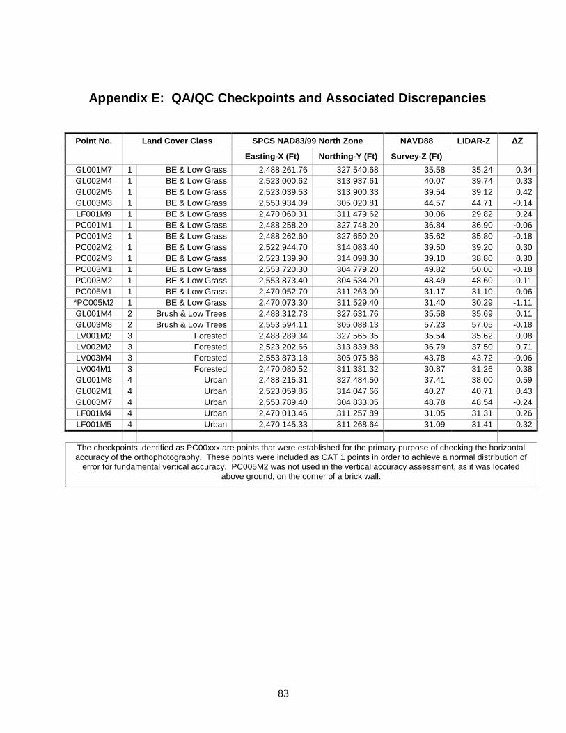
83
Appendix E: QA/QC Checkpoints and Associated Discrepancies
Point No. Land Cover Class SPCS NAD83/99 North Zone NAVD88 LIDAR-Z ΔZ
Easting-X (Ft) Northing-Y (Ft) Survey-Z (Ft)
GL001M7 1 BE & Low Grass 2,488,261.76 327,540.68 35.58 35.24 0.34
GL002M4 1 BE & Low Grass 2,523,000.62 313,937.61 40.07 39.74 0.33
GL002M5 1 BE & Low Grass 2,523,039.53 313,900.33 39.54 39.12 0.42
GL003M3 1 BE & Low Grass 2,553,934.09 305,020.81 44.57 44.71 -0.14
LF001M9 1 BE & Low Grass 2,470,060.31 311,479.62 30.06 29.82 0.24
PC001M1 1 BE & Low Grass 2,488,258.20 327,748.20 36.84 36.90 -0.06
PC001M2 1 BE & Low Grass 2,488,262.60 327,650.20 35.62 35.80 -0.18
PC002M2 1 BE & Low Grass 2,522,944.70 314,083.40 39.50 39.20 0.30
PC002M3 1 BE & Low Grass 2,523,139.90 314,098.30 39.10 38.80 0.30
PC003M1 1 BE & Low Grass 2,553,720.30 304,779.20 49.82 50.00 -0.18
PC003M2 1 BE & Low Grass 2,553,873.40 304,534.20 48.49 48.60 -0.11
PC005M1 1 BE & Low Grass 2,470,052.70 311,263.00 31.17 31.10 0.06
*PC005M2 1 BE & Low Grass 2,470,073.30 311,529.40 31.40 30.29 -1.11
GL001M4 2 Brush & Low Trees 2,488,312.78 327,631.76 35.58 35.69 0.11
GL003M8 2 Brush & Low Trees 2,553,594.11 305,088.13 57.23 57.05 -0.18
LV001M2 3 Forested 2,488,289.34 327,565.35 35.54 35.62 0.08
LV002M2 3 Forested 2,523,202.66 313,839.88 36.79 37.50 0.71
LV003M4 3 Forested 2,553,873.18 305,075.88 43.78 43.72 -0.06
LV004M1 3 Forested 2,470,080.52 311,331.32 30.87 31.26 0.38
GL001M8 4 Urban 2,488,215.31 327,484.50 37.41 38.00 0.59
GL002M1 4 Urban 2,523,059.86 314,047.66 40.27 40.71 0.43
GL003M7 4 Urban 2,553,789.40 304,833.05 48.78 48.54 -0.24
LF001M4 4 Urban 2,470,013.46 311,257.89 31.05 31.31 0.26
LF001M5 4 Urban 2,470,145.33 311,268.64 31.09 31.41 0.32
The checkpoints identified as PC00xxx are points that were established for the primary purpose of checking the horizontal accuracy of the orthophotography. These points were included as CAT 1 points in order to achieve a normal distribution of
error for fundamental vertical accuracy. PC005M2 was not used in the vertical accuracy assessment, as it was located above ground, on the corner of a brick wall.
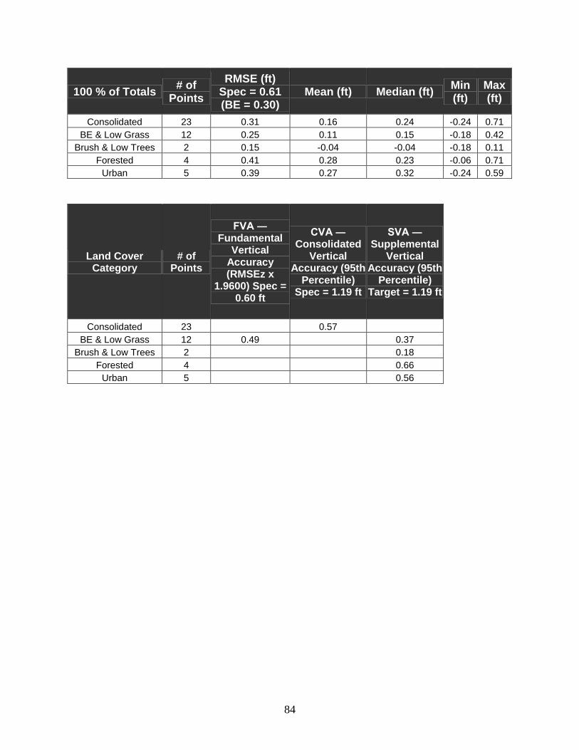
84
100 % of Totals # of
Points
RMSE (ft) Spec = 0.61 (BE = 0.30)
Mean (ft) Median (ft) Min (ft)
Max (ft)
Consolidated 23 0.31 0.16 0.24 -0.24 0.71
BE & Low Grass 12 0.25 0.11 0.15 -0.18 0.42
Brush & Low Trees 2 0.15 -0.04 -0.04 -0.18 0.11
Forested 4 0.41 0.28 0.23 -0.06 0.71
Urban 5 0.39 0.27 0.32 -0.24 0.59
Land Cover Category
# of Points
FVA ― Fundamental
Vertical Accuracy (RMSEz x
1.9600) Spec = 0.60 ft
CVA ― Consolidated
Vertical Accuracy (95th
Percentile) Spec = 1.19 ft
SVA ― Supplemental
Vertical Accuracy (95th
Percentile) Target = 1.19 ft
Consolidated 23 0.57
BE & Low Grass 12 0.49 0.37
Brush & Low Trees 2 0.18
Forested 4 0.66
Urban 5 0.56
85
Appendix F: LiDAR Vertical Accuracy Report
Vertical Accuracy Assessment Report
2007 LiDAR Bare-Earth Dataset for
Suwannee River Water Management District, Florida – SRWMD Contract #06/07-268
Date: March 22, 2010
References: A ― State of Florida Division of Emergency Management (FDEM), Contract Number 07-
HS-34-14-00-22-469, Task Order Number 20070525-492718a
B ― Part 3: National Standard for Spatial Data Accuracy (NSSDA), “Geospatial Positioning
Accuracy Standards,” published by the Federal Geographic Data Committee (FGDC), 1998
C ― Appendix A, Guidance for Aerial Mapping and Surveying, “Guidelines and
Specifications for Flood Hazard Mapping Partners,” published by the Federal Emergency
Management Agency (FEMA), April 2003
D ― Guidelines for Digital Elevation Data, Version 1.0, published by the National Digital
Elevation Program (NDEP), May 10, 2004
E ― ASPRS Guidelines, Vertical Accuracy Reporting for Lidar Data, published by the
American Society for Photogrammetry and Remote Sensing (ASPRS), May 24, 2004
Background
FDEM Guidance: Reference A tasked PDS to validate the bare-earth LiDAR dataset of SRWMD, FL,
both quantitatively (for accuracy) and qualitatively (for usability). This report addresses the vertical
accuracy assessment only, for which FDEM‟s major specifications are summarized as follows:
Vertical accuracy: < 0.30 feet RMSEz = < 0.60 feet vertical accuracy at 95% confidence level,
tested in flat, non-vegetated terrain only, employing NSSDA procedures in Reference B.
Validation that the data also satisfies FEMA requirements in Reference C.
Vertical units (orthometric heights) are in US Survey Feet, NAVD88.
NSSDA Guidance: Section 3.2.2 of Reference B specifies: “A minimum of 20 check points shall be
tested, distributed to reflect the geographic area of interest and the distribution of error in the dataset.
When 20 points are tested, the 95% confidence level allows one point to fail the threshold given in
product specifications.”
FEMA Guidance: Section A.8.6 of Reference C specifies the following LiDAR testing requirement for
data to be used by the National Flood Insurance Program (NFIP): “For the NFIP, TINs (and DEMs
derived there from) should normally have a maximum RMSE of 18.5 centimeters, equivalent to 2-foot
contours, in flat terrain; and a maximum RMSE of 37 centimeters, equivalent to 4-foot contours, in
rolling to hilly terrain. The Mapping Partner shall field verify the vertical accuracy of this TIN to ensure
that the 18.5- or 37.0-centimeter RMSE requirement is satisfied for all major vegetation categories that
predominate within the floodplain being studied … The assigned Mapping Partner shall separately
evaluate and report on the TIN accuracy for the main categories of ground cover in the study area,
including the following: [followed by explanations of seven potential categories]… Ground cover
Categories 1 through 5 are fairly common everywhere … The assigned Mapping Partner shall select a
minimum of 20 test points for each major vegetation category identified. Therefore, a minimum of 60
test points shall be selected for three (minimum) major land cover categories, 80 test points for four major
categories, and so on.”
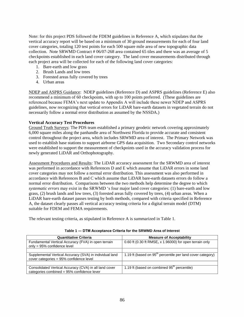
86
Note: for this project PDS followed the FDEM guidelines in Reference A, which stipulates that the
vertical accuracy report will be based on a minimum of 30 ground measurements for each of four land
cover categories, totaling 120 test points for each 500 square mile area of new topographic data
collection. Note SRWMD Contract # 06/07-268 area contained 65 tiles and there was an average of 5
checkpoints established in each land cover category. The land cover measurements distributed through
each project area will be collected for each of the following land cover categories:
1. Bare-earth and low grass
2. Brush Lands and low trees
3. Forested areas fully covered by trees
4. Urban areas
NDEP and ASPRS Guidance: NDEP guidelines (Reference D) and ASPRS guidelines (Reference E) also
recommend a minimum of 60 checkpoints, with up to 100 points preferred. (These guidelines are
referenced because FEMA‟s next update to Appendix A will include these newer NDEP and ASPRS
guidelines, now recognizing that vertical errors for LiDAR bare-earth datasets in vegetated terrain do not
necessarily follow a normal error distribution as assumed by the NSSDA.)
Vertical Accuracy Test Procedures
Ground Truth Surveys: The PDS team established a primary geodetic network covering approximately
6,000 square miles along the panhandle area of Northwest Florida to provide accurate and consistent
control throughout the project area, which includes SRWMD area of interest. The Primary Network was
used to establish base stations to support airborne GPS data acquisition. Two Secondary control networks
were established to support the measurement of checkpoints used in the accuracy validation process for
newly generated LiDAR and Orthophotography.
Assessment Procedures and Results: The LiDAR accuracy assessment for the SRWMD area of interest
was performed in accordance with References D and E which assume that LiDAR errors in some land
cover categories may not follow a normal error distribution. This assessment was also performed in
accordance with References B and C which assume that LiDAR bare-earth datasets errors do follow a
normal error distribution. Comparisons between the two methods help determine the degree to which
systematic errors may exist in the SRWMD „s four major land cover categories: (1) bare-earth and low
grass, (2) brush lands and low trees, (3) forested areas fully covered by trees, (4) urban areas. When a
LiDAR bare-earth dataset passes testing by both methods, compared with criteria specified in Reference
A, the dataset clearly passes all vertical accuracy testing criteria for a digital terrain model (DTM)
suitable for FDEM and FEMA requirements.
The relevant testing criteria, as stipulated in Reference A is summarized in Table 1.
Table 1 ― DTM Acceptance Criteria for the SRWMD Area of Interest
Quantitative Criteria Measure of Acceptability
Fundamental Vertical Accuracy (FVA) in open terrain only = 95% confidence level
0.60 ft (0.30 ft RMSEz x 1.96000) for open terrain only
Supplemental Vertical Accuracy (SVA) in individual land cover categories = 95% confidence level
1.19 ft (based on 95th
percentile per land cover category)
Consolidated Vertical Accuracy (CVA) in all land cover categories combined = 95% confidence lever
1.19 ft (based on combined 95th
percentile)
87
Vertical Accuracy Testing in Accordance with NDEP and ASPRS Procedures
References D and E specify the mandatory determination of Fundamental Vertical Accuracy (FVA) and
the optional determination of Supplemental Vertical Accuracy (SVA) and Consolidated Vertical
Accuracy (CVA). FVA determines how well the LiDAR sensor performed in category (1), open terrain,
where errors are random and normally distributed; whereas SVA determines how well the vegetation
classification algorithms worked in land cover categories (2) and (3) where LiDAR elevations are often
higher than surveyed elevations and category (4) where LiDAR elevations are often lower.
FVA is determined with check points located only in land cover category (1), open terrain (grass, dirt,
sand, and/or rocks), where there is a very high probability that the LiDAR sensor will have detected the
bare-earth ground surface and where random errors are expected to follow a normal error distribution. The
FVA determines how well the calibrated LiDAR sensor performed. With a normal error distribution, the
vertical accuracy at the 95% confidence level is computed as the vertical root mean square error (RMSEz)
of the checkpoints x 1.9600, as specified in Reference B. For SRWMD, for which floodplains are
essentially flat, FDEM required the FVA to be 0.60 ft (18.29 cm) at the 95% confidence level (based on
an RMSEz of 0.30 ft (9.14 cm), equivalent to 1 ft contours).
CVA is determined with all checkpoints in all land cover categories combined where there is a possibility
that the LiDAR sensor and post-processing may yield elevation errors that do not follow a normal error
distribution. CVA at the 95% confidence level equals the 95th percentile error for all checkpoints in all
land cover categories combined. FDEM‟s CVA standard is 1.19 ft at the 95% confidence level. The CVA
is accompanied by a listing of the 5% outliers that are larger than the 95th percentile used to compute the
CVA; these are always the largest outliers that may depart from a normal error distribution. Here,
Accuracyz differs from CVA because Accuracyz assumes elevation errors follow a normal error
distribution where RMSE procedures are valid, whereas CVA assumes LiDAR errors may not follow a
normal error distribution in vegetated categories, making the RMSE process invalid.
SVA is determined separately for each individual land cover category, again recognizing that the LiDAR
sensor and post-processing may yield elevation errors that do not follow a normal error distribution, and
where discrepancies can be used to identify the nature of systematic errors by land cover category. For
each land cover category, the SVA at the 95% confidence level equals the 95th percentile error for all
checkpoints in each individual land cover category. SVA statistics are calculated individually for bare-
earth and low grass, brush lands and low trees, forested areas, and urban areas, in order to facilitate the
analysis of the data based on each of these land cover categories that exist within SRWMD area of
interest. The SVA criteria in Table 1 (1.19 ft at the 95% confidence level for each category) are target
values only and are not mandatory; it is common for some SVA criteria to fail individual target values,
yet satisfy FEMA‟s mandatory CVA criterion.
QA/QC Steps: The primary QA/QC steps used by PDS were as follows:
1. PDS surveyed "ground truth" QA/QC vertical checkpoints in accordance with guidance in references
B, C, D and E. Figure 1 shows the location of “cluster areas” where PDS attempted to survey a
minimum of 5 QA/QC checkpoints in each of the four land cover categories. Some clusters may not
include points from all cover categories. The final totals were 12 checkpoints in bare-earth and low
grass; 2 checkpoints in brush and low trees; 4 checkpoints in forested areas; and 5 checkpoints in
urban areas, for a total of 119 checkpoints. Note 7 ortho checkpoints were added to the bare-earth
and low grass classification. 2. Next, PDS interpolated the bare-earth LiDAR DTM to provide the z-value for each of the 23
checkpoints.
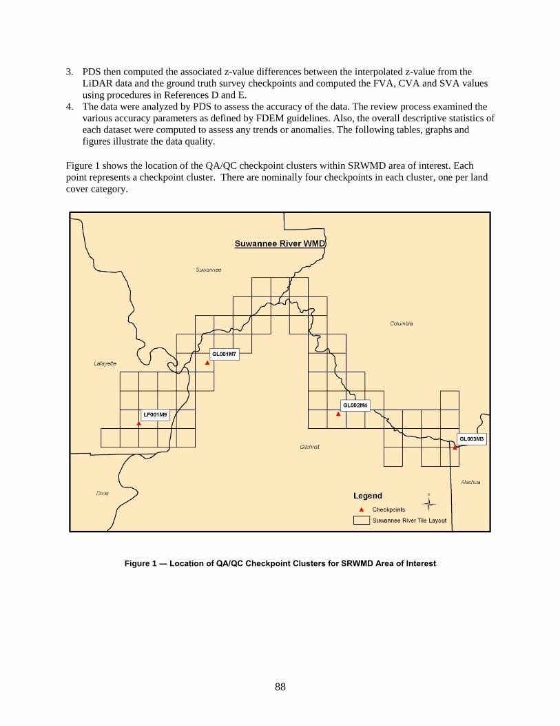
88
3. PDS then computed the associated z-value differences between the interpolated z-value from the
LiDAR data and the ground truth survey checkpoints and computed the FVA, CVA and SVA values
using procedures in References D and E.
4. The data were analyzed by PDS to assess the accuracy of the data. The review process examined the
various accuracy parameters as defined by FDEM guidelines. Also, the overall descriptive statistics of
each dataset were computed to assess any trends or anomalies. The following tables, graphs and
figures illustrate the data quality.
Figure 1 shows the location of the QA/QC checkpoint clusters within SRWMD area of interest. Each
point represents a checkpoint cluster. There are nominally four checkpoints in each cluster, one per land
cover category.
Figure 1 ― Location of QA/QC Checkpoint Clusters for SRWMD Area of Interest
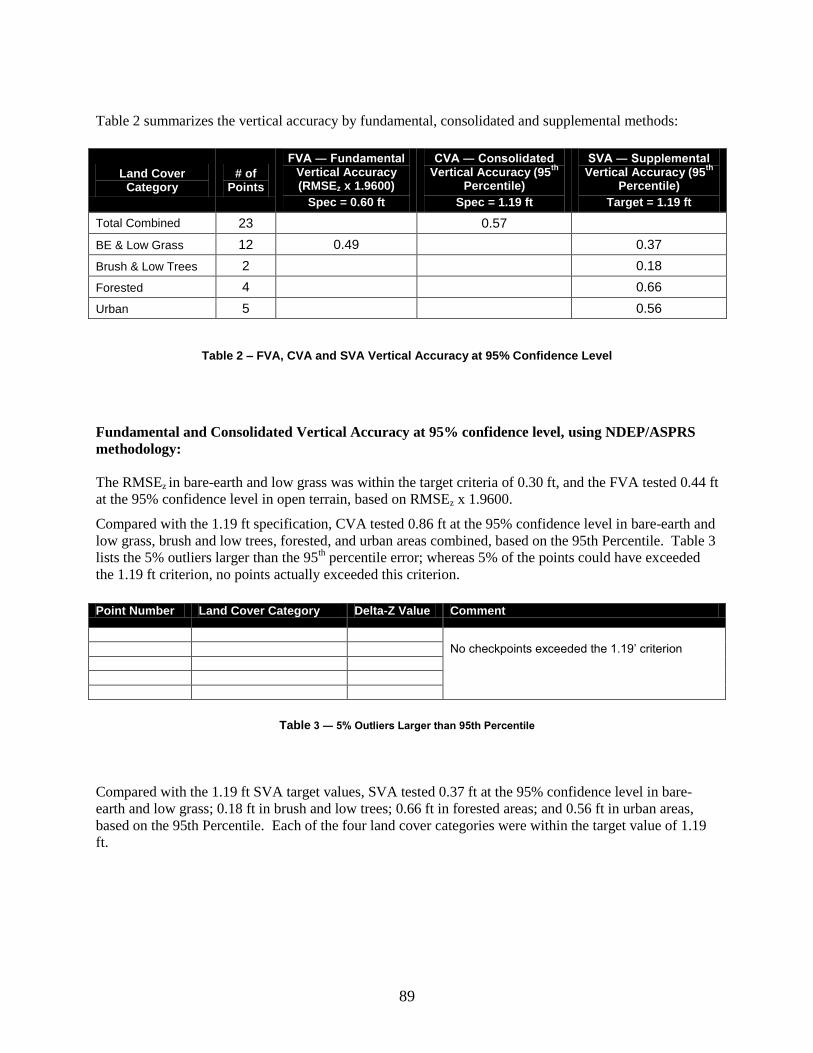
89
Table 2 summarizes the vertical accuracy by fundamental, consolidated and supplemental methods:
Table 2 – FVA, CVA and SVA Vertical Accuracy at 95% Confidence Level
Fundamental and Consolidated Vertical Accuracy at 95% confidence level, using NDEP/ASPRS
methodology:
The RMSEz in bare-earth and low grass was within the target criteria of 0.30 ft, and the FVA tested 0.44 ft
at the 95% confidence level in open terrain, based on RMSEz x 1.9600.
Compared with the 1.19 ft specification, CVA tested 0.86 ft at the 95% confidence level in bare-earth and
low grass, brush and low trees, forested, and urban areas combined, based on the 95th Percentile. Table 3
lists the 5% outliers larger than the 95th percentile error; whereas 5% of the points could have exceeded
the 1.19 ft criterion, no points actually exceeded this criterion.
Table 3 ― 5% Outliers Larger than 95th Percentile
Compared with the 1.19 ft SVA target values, SVA tested 0.37 ft at the 95% confidence level in bare-
earth and low grass; 0.18 ft in brush and low trees; 0.66 ft in forested areas; and 0.56 ft in urban areas,
based on the 95th Percentile. Each of the four land cover categories were within the target value of 1.19
ft.
Land Cover Category
# of Points
FVA ― Fundamental Vertical Accuracy (RMSEz x 1.9600)
Spec = 0.60 ft
CVA ― Consolidated Vertical Accuracy (95
th
Percentile)
Spec = 1.19 ft
SVA ― Supplemental Vertical Accuracy (95
th
Percentile)
Target = 1.19 ft
Total Combined 23 0.57
BE & Low Grass 12 0.49 0.37
Brush & Low Trees 2 0.18
Forested 4 0.66
Urban 5 0.56
Point Number Land Cover Category Delta-Z Value Comment
No checkpoints exceeded the 1.19’ criterion
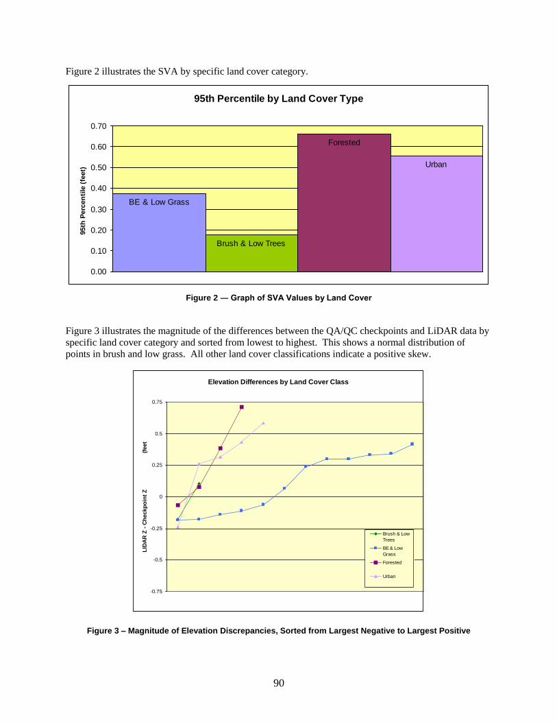
90
Elevation Differences by Land Cover Class
-0.75
-0.5
-0.25
0
0.25
0.5
0.75
LID
AR
Z -
Ch
eckp
oin
t Z
(fe
et
Brush & Low
Trees
BE & Low
Grass
Forested
Urban
Figure 2 illustrates the SVA by specific land cover category.
95th Percentile by Land Cover Type
BE & Low Grass
Brush & Low Trees
Forested
Urban
0.00
0.10
0.20
0.30
0.40
0.50
0.60
0.70
95th
Perc
en
tile
(fe
et)
Figure 2 ― Graph of SVA Values by Land Cover
Figure 3 illustrates the magnitude of the differences between the QA/QC checkpoints and LiDAR data by
specific land cover category and sorted from lowest to highest. This shows a normal distribution of
points in brush and low grass. All other land cover classifications indicate a positive skew.
Vertical Accuracy Testing in Accordance with NSSDA and FEMA Procedures
Figure 3 – Magnitude of Elevation Discrepancies, Sorted from Largest Negative to Largest Positive
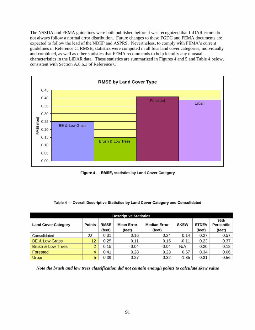
91
The NSSDA and FEMA guidelines were both published before it was recognized that LiDAR errors do
not always follow a normal error distribution. Future changes to these FGDC and FEMA documents are
expected to follow the lead of the NDEP and ASPRS. Nevertheless, to comply with FEMA‟s current
guidelines in Reference C, RMSEz statistics were computed in all four land cover categories, individually
and combined, as well as other statistics that FEMA recommends to help identify any unusual
characteristics in the LiDAR data. These statistics are summarized in Figures 4 and 5 and Table 4 below,
consistent with Section A.8.6.3 of Reference C.
RMSE by Land Cover Type
BE & Low Grass
Brush & Low Trees
ForestedUrban
0.00
0.05
0.10
0.15
0.20
0.25
0.30
0.35
0.40
0.45
RM
SE
(fe
et)
Figure 4 ― RMSEz statistics by Land Cover Category
Table 4 ― Overall Descriptive Statistics by Land Cover Category and Consolidated
Descriptive Statistics
Land Cover Category Points RMSE Mean Error Median Error SKEW STDEV 95th
Percentile
(feet) (feet) (feet) (feet) (feet)
Consolidated 23 0.31 0.16 0.24 0.14 0.27 0.57
BE & Low Grass 12 0.25 0.11 0.15 -0.11 0.23 0.37
Brush & Low Trees 2 0.15 -0.04 -0.04 N/A 0.20 0.18
Forested 4 0.41 0.28 0.23 0.57 0.34 0.66
Urban 5 0.39 0.27 0.32 -1.35 0.31 0.56
Note the brush and low trees classification did not contain enough points to calculate skew value
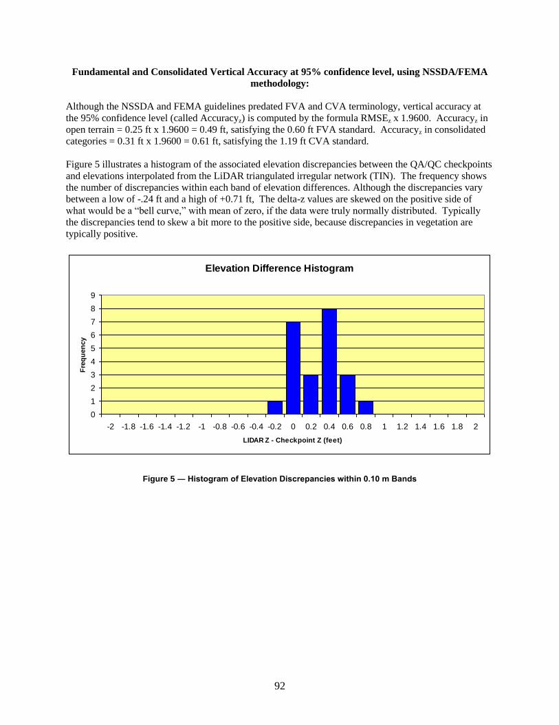
92
Fundamental and Consolidated Vertical Accuracy at 95% confidence level, using NSSDA/FEMA
methodology:
Although the NSSDA and FEMA guidelines predated FVA and CVA terminology, vertical accuracy at
the 95% confidence level (called Accuracyz) is computed by the formula RMSEz x 1.9600. Accuracyz in
open terrain = 0.25 ft x 1.9600 = 0.49 ft, satisfying the 0.60 ft FVA standard. Accuracyz in consolidated
categories = 0.31 ft x 1.9600 = 0.61 ft, satisfying the 1.19 ft CVA standard.
Figure 5 illustrates a histogram of the associated elevation discrepancies between the QA/QC checkpoints
and elevations interpolated from the LiDAR triangulated irregular network (TIN). The frequency shows
the number of discrepancies within each band of elevation differences. Although the discrepancies vary
between a low of -.24 ft and a high of +0.71 ft, The delta-z values are skewed on the positive side of
what would be a “bell curve,” with mean of zero, if the data were truly normally distributed. Typically
the discrepancies tend to skew a bit more to the positive side, because discrepancies in vegetation are
typically positive.
Elevation Difference Histogram
0
1
2
3
4
5
6
7
8
9
-2 -1.8 -1.6 -1.4 -1.2 -1 -0.8 -0.6 -0.4 -0.2 0 0.2 0.4 0.6 0.8 1 1.2 1.4 1.6 1.8 2
LIDAR Z - Checkpoint Z (feet)
Fre
qu
en
cy
Figure 5 ― Histogram of Elevation Discrepancies within 0.10 m Bands
93
Conclusions
Based on the vertical accuracy testing conducted by PDS, the undersigned certifies that the LiDAR
dataset for SRWMD, Florida satisfies the criteria established by Reference A:
Based on NSSDA, FEMA, NDEP and ASPRS methodology: Tested 0.49’ vertical accuracy
at 95% confidence level in open terrain.
Based on NSSDA and FEMA methodology: Tested 0.61’ vertical accuracy at 95%
confidence level in all land cover categories combined.
David F. Maune, Ph.D., PSM, PS, GS, CP
QA/QC Manager
94
Appendix G: LiDAR Qualitative Assessment Report
References:
A ─ State of Florida Division of Emergency Management (FDEM), Contract Number 07-HS-34-14-00-
22-469, Task Order Number 20070525-492718a
B ─ Part 3: National Standard for Spatial Data Accuracy (NSSDA), “Geospatial Positioning Accuracy
Standards,” published by the Federal Geographic Data Committee (FGDC), 1998
C ─ Appendix A, Guidance for Aerial Mapping and Surveying, “Guidelines and Specifications for Flood
Hazard Mapping Partners,” published by the Federal Emergency Management Agency (FEMA),
April 2003
D ─ Guidelines for Digital Elevation Data, Version 1.0, published by the National Digital Elevation
Program (NDEP), May 10, 2004
E ─ ASPRS Guidelines, Vertical Accuracy Reporting for LiDAR Data, published by the American Society
for Photogrammetry and Remote Sensing (ASPRS), May 24, 2004
Qualitative Assessment The PDS qualitative assessment utilizes a combination of statistical analysis and interpretative
methodology to assess the quality of the data for a bare-earth digital terrain model (DTM). This process
looks for anomalies in the data and also identifies areas where man-made structures or vegetation points
may not have been classified properly to produce a bare-earth model. Overall the data are of good quality
and should satisfy most users for an accurate bare-earth elevation data product.
Overview Within this review of the LiDAR data, two fundamental questions were addressed:
Did the LiDAR system perform to specifications?
Did the vegetation removal process yield desirable results for the intended bare-earth terrain
product?
Mapping standards today address the quality of data by quantitative methods. If the data are tested and
found to be within the desired accuracy standard, then the data set is typically accepted. Now with the
proliferation of LiDAR, new issues arise due to the vast amount of data. Unlike photogrammetrically-
derived DEMs where point spacing can be eight meters or more, the nominal LiDAR point spacing for
this project was 0.7 meters, and with the PDS team‟s 50% sidelap between flightlines, the nominal overall
point density was designed to be approximately 4 points per square meter. The end result is that millions
of elevation points are measured to a level of accuracy previously unseen for traditional, elevation
mapping technologies, and vegetated areas are measured that would be nearly impossible to survey by
other means. The downside is that with millions of points, the data set is statistically bound to have some
errors both in the measurement process and in the artifact removal process.
As previously stated, the quantitative analysis addresses the quality of the data based on absolute
accuracy. This accuracy is directly tied to the comparison of the discreet measurement of the survey
checkpoints and that of the interpolated value within the three closest LiDAR points that constitute the
vertices of a three-dimensional triangular face of the TIN. Therefore, the end result is that only a small
sample of the LiDAR data is actually tested. However there is an increased level of confidence with
LiDAR data due to the relative accuracy. This relative accuracy in turn is based on how well one LiDAR
point "fits" in comparison to the next contiguous LiDAR measurement. Once the absolute and relative

95
accuracy has been ascertained, the next stage is to address the cleanliness of the data for a bare-earth
DTM.
By using survey checkpoints to compare the data, the absolute accuracy is verified, but this also allows us
to understand if the artifact removal process was performed correctly. To reiterate the quantitative
approach, if the LiDAR sensor operated correctly over open terrain areas, then it most likely operated
correctly over the vegetated areas. This does not mean that the bare-earth was measured, but that the
elevations surveyed are most likely accurate (including elevations of treetops, rooftops, etc.). In the event
that the LiDAR pulse filtered through the vegetation and was able to measure the true surface (as well as
measurements on the surrounding vegetation) then the level of accuracy of the vegetation removal process
can be tested as a by-product.
To fully address the data for overall accuracy and quality, the level of cleanliness (or removal of above-
ground artifacts) is paramount. Since there are currently no effective automated testing procedures to
measure cleanliness, PDS employs a combination of statistical and visualization processes. This includes
creating pseudo image products such as LiDAR orthos produced from the intensity returns, Triangular
Irregular Network (TIN)‟s, Digital Elevation Models (DEM) and 3-dimensional models. By creating
multiple images and using overlay techniques, not only can potential errors be found, but the PDS team
can also find where the data meets and exceeds expectations. This report will present representative
examples where the LiDAR and post processing had issues as well as examples of where the LiDAR
performed well.
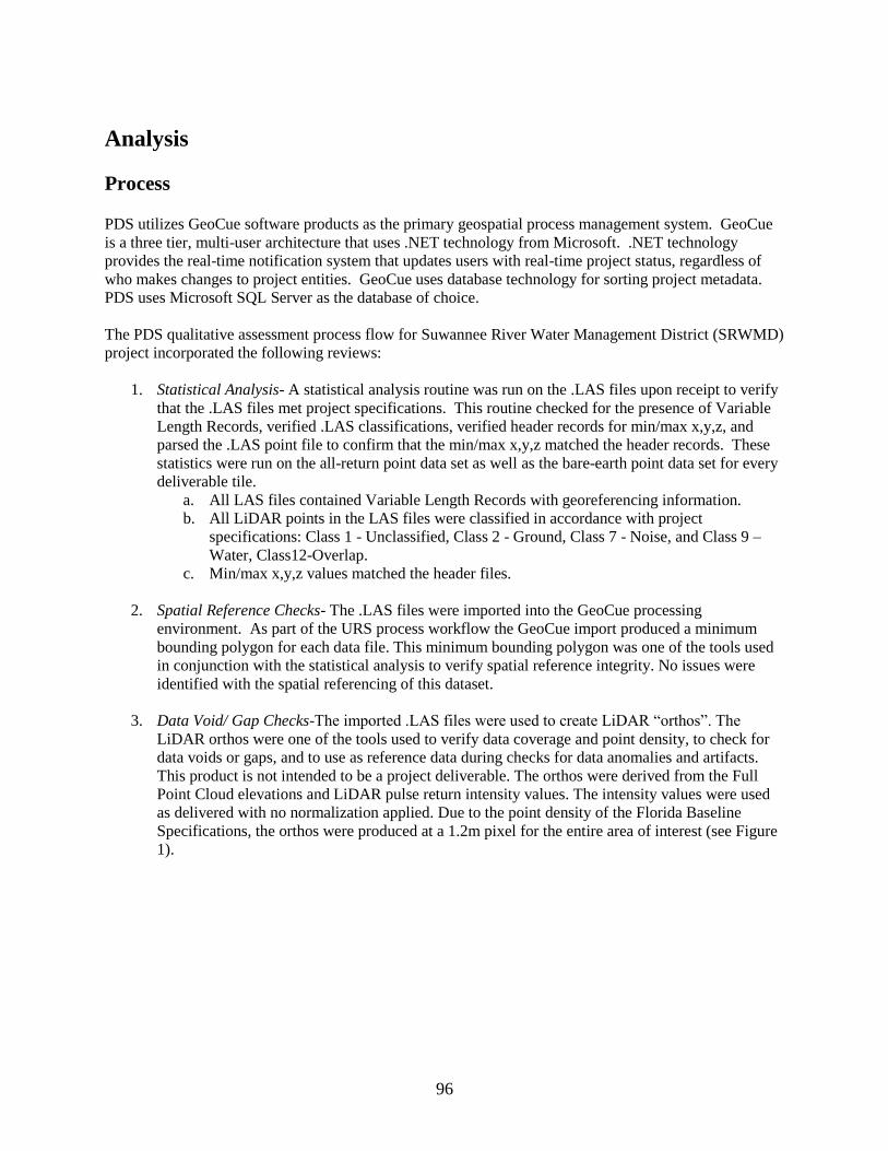
96
Analysis
Process PDS utilizes GeoCue software products as the primary geospatial process management system. GeoCue
is a three tier, multi-user architecture that uses .NET technology from Microsoft. .NET technology
provides the real-time notification system that updates users with real-time project status, regardless of
who makes changes to project entities. GeoCue uses database technology for sorting project metadata.
PDS uses Microsoft SQL Server as the database of choice.
The PDS qualitative assessment process flow for Suwannee River Water Management District (SRWMD)
project incorporated the following reviews:
1. Statistical Analysis- A statistical analysis routine was run on the .LAS files upon receipt to verify
that the .LAS files met project specifications. This routine checked for the presence of Variable
Length Records, verified .LAS classifications, verified header records for min/max x,y,z, and
parsed the .LAS point file to confirm that the min/max x,y,z matched the header records. These
statistics were run on the all-return point data set as well as the bare-earth point data set for every
deliverable tile.
a. All LAS files contained Variable Length Records with georeferencing information.
b. All LiDAR points in the LAS files were classified in accordance with project
specifications: Class 1 - Unclassified, Class 2 - Ground, Class 7 - Noise, and Class 9 –
Water, Class12-Overlap.
c. Min/max x,y,z values matched the header files.
2. Spatial Reference Checks- The .LAS files were imported into the GeoCue processing
environment. As part of the URS process workflow the GeoCue import produced a minimum
bounding polygon for each data file. This minimum bounding polygon was one of the tools used
in conjunction with the statistical analysis to verify spatial reference integrity. No issues were
identified with the spatial referencing of this dataset.
3. Data Void/ Gap Checks-The imported .LAS files were used to create LiDAR “orthos”. The
LiDAR orthos were one of the tools used to verify data coverage and point density, to check for
data voids or gaps, and to use as reference data during checks for data anomalies and artifacts.
This product is not intended to be a project deliverable. The orthos were derived from the Full
Point Cloud elevations and LiDAR pulse return intensity values. The intensity values were used
as delivered with no normalization applied. Due to the point density of the Florida Baseline
Specifications, the orthos were produced at a 1.2m pixel for the entire area of interest (see Figure
1).
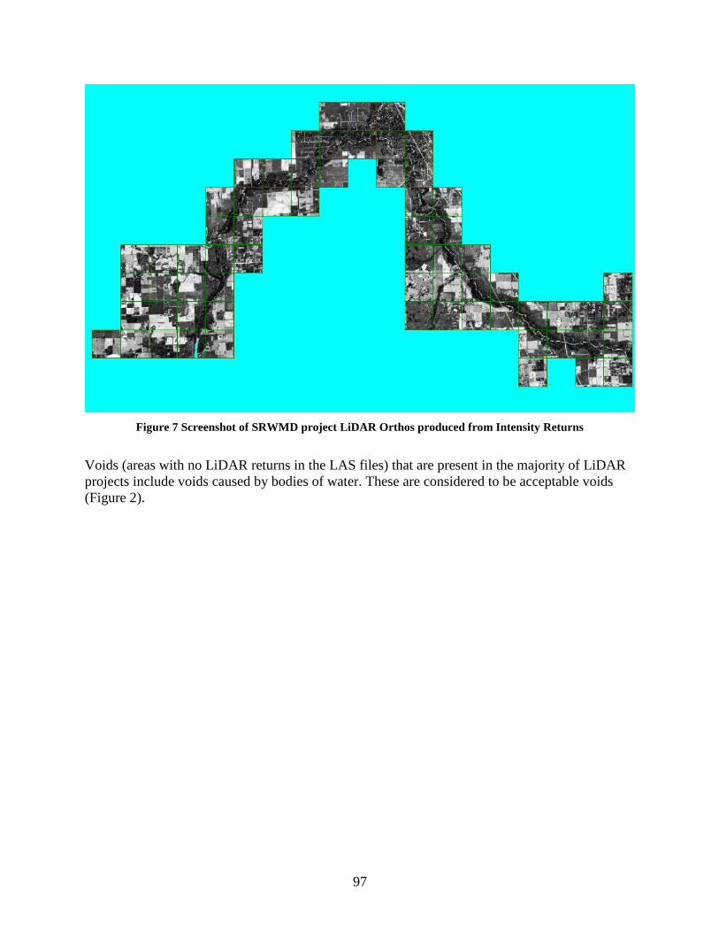
97
Figure 7 Screenshot of SRWMD project LiDAR Orthos produced from Intensity Returns
Voids (areas with no LiDAR returns in the LAS files) that are present in the majority of LiDAR
projects include voids caused by bodies of water. These are considered to be acceptable voids
(Figure 2).
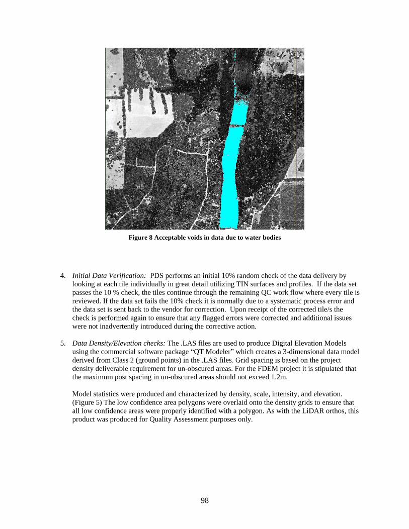
98
Figure 8 Acceptable voids in data due to water bodies
4. Initial Data Verification: PDS performs an initial 10% random check of the data delivery by
looking at each tile individually in great detail utilizing TIN surfaces and profiles. If the data set
passes the 10 % check, the tiles continue through the remaining QC work flow where every tile is
reviewed. If the data set fails the 10% check it is normally due to a systematic process error and
the data set is sent back to the vendor for correction. Upon receipt of the corrected tile/s the
check is performed again to ensure that any flagged errors were corrected and additional issues
were not inadvertently introduced during the corrective action.
5. Data Density/Elevation checks: The .LAS files are used to produce Digital Elevation Models
using the commercial software package “QT Modeler” which creates a 3-dimensional data model
derived from Class 2 (ground points) in the .LAS files. Grid spacing is based on the project
density deliverable requirement for un-obscured areas. For the FDEM project it is stipulated that
the maximum post spacing in un-obscured areas should not exceed 1.2m.
Model statistics were produced and characterized by density, scale, intensity, and elevation.
(Figure 5) The low confidence area polygons were overlaid onto the density grids to ensure that
all low confidence areas were properly identified with a polygon. As with the LiDAR orthos, this
product was produced for Quality Assessment purposes only.
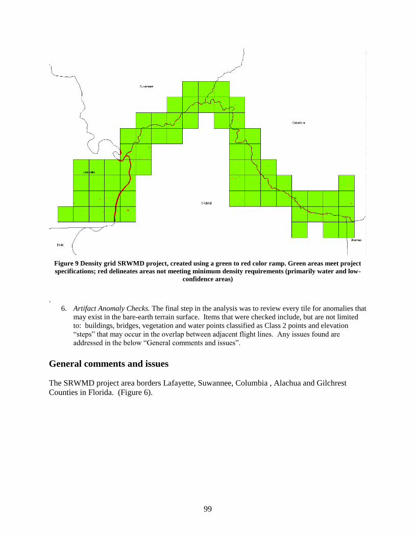
99
Figure 9 Density grid SRWMD project, created using a green to red color ramp. Green areas meet project
specifications; red delineates areas not meeting minimum density requirements (primarily water and low-
confidence areas)
.
6. Artifact Anomaly Checks. The final step in the analysis was to review every tile for anomalies that
may exist in the bare-earth terrain surface. Items that were checked include, but are not limited
to: buildings, bridges, vegetation and water points classified as Class 2 points and elevation
“steps” that may occur in the overlap between adjacent flight lines. Any issues found are
addressed in the below “General comments and issues”.
General comments and issues
The SRWMD project area borders Lafayette, Suwannee, Columbia , Alachua and Gilchrest
Counties in Florida. (Figure 6).
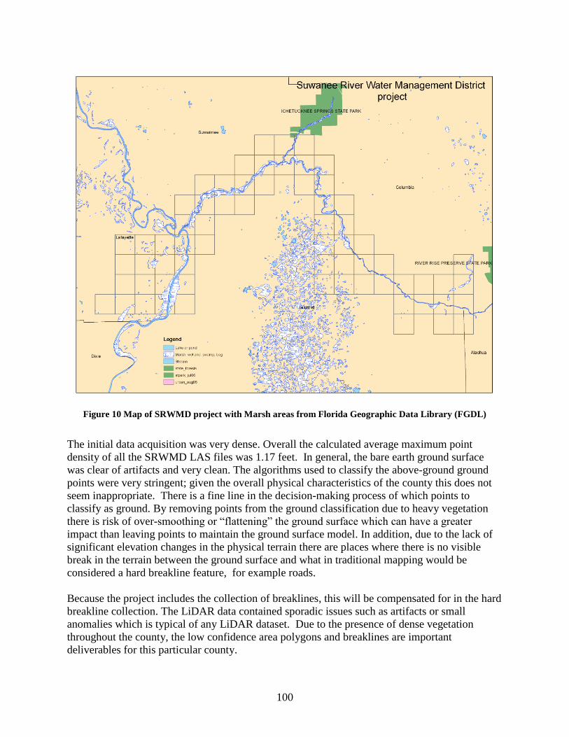
100
Figure 10 Map of SRWMD project with Marsh areas from Florida Geographic Data Library (FGDL)
The initial data acquisition was very dense. Overall the calculated average maximum point
density of all the SRWMD LAS files was 1.17 feet. In general, the bare earth ground surface
was clear of artifacts and very clean. The algorithms used to classify the above-ground ground
points were very stringent; given the overall physical characteristics of the county this does not
seem inappropriate. There is a fine line in the decision-making process of which points to
classify as ground. By removing points from the ground classification due to heavy vegetation
there is risk of over-smoothing or “flattening” the ground surface which can have a greater
impact than leaving points to maintain the ground surface model. In addition, due to the lack of
significant elevation changes in the physical terrain there are places where there is no visible
break in the terrain between the ground surface and what in traditional mapping would be
considered a hard breakline feature, for example roads.
Because the project includes the collection of breaklines, this will be compensated for in the hard
breakline collection. The LiDAR data contained sporadic issues such as artifacts or small
anomalies which is typical of any LiDAR dataset. Due to the presence of dense vegetation
throughout the county, the low confidence area polygons and breaklines are important
deliverables for this particular county.
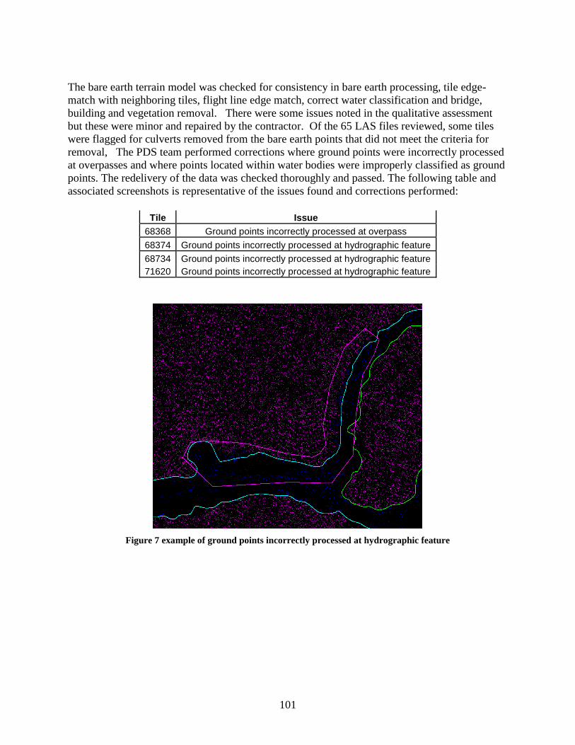
101
The bare earth terrain model was checked for consistency in bare earth processing, tile edge-
match with neighboring tiles, flight line edge match, correct water classification and bridge,
building and vegetation removal. There were some issues noted in the qualitative assessment
but these were minor and repaired by the contractor. Of the 65 LAS files reviewed, some tiles
were flagged for culverts removed from the bare earth points that did not meet the criteria for
removal, The PDS team performed corrections where ground points were incorrectly processed
at overpasses and where points located within water bodies were improperly classified as ground
points. The redelivery of the data was checked thoroughly and passed. The following table and
associated screenshots is representative of the issues found and corrections performed:
Tile Issue
68368 Ground points incorrectly processed at overpass
68374 Ground points incorrectly processed at hydrographic feature
68734 Ground points incorrectly processed at hydrographic feature
71620 Ground points incorrectly processed at hydrographic feature
Figure 7 example of ground points incorrectly processed at hydrographic feature
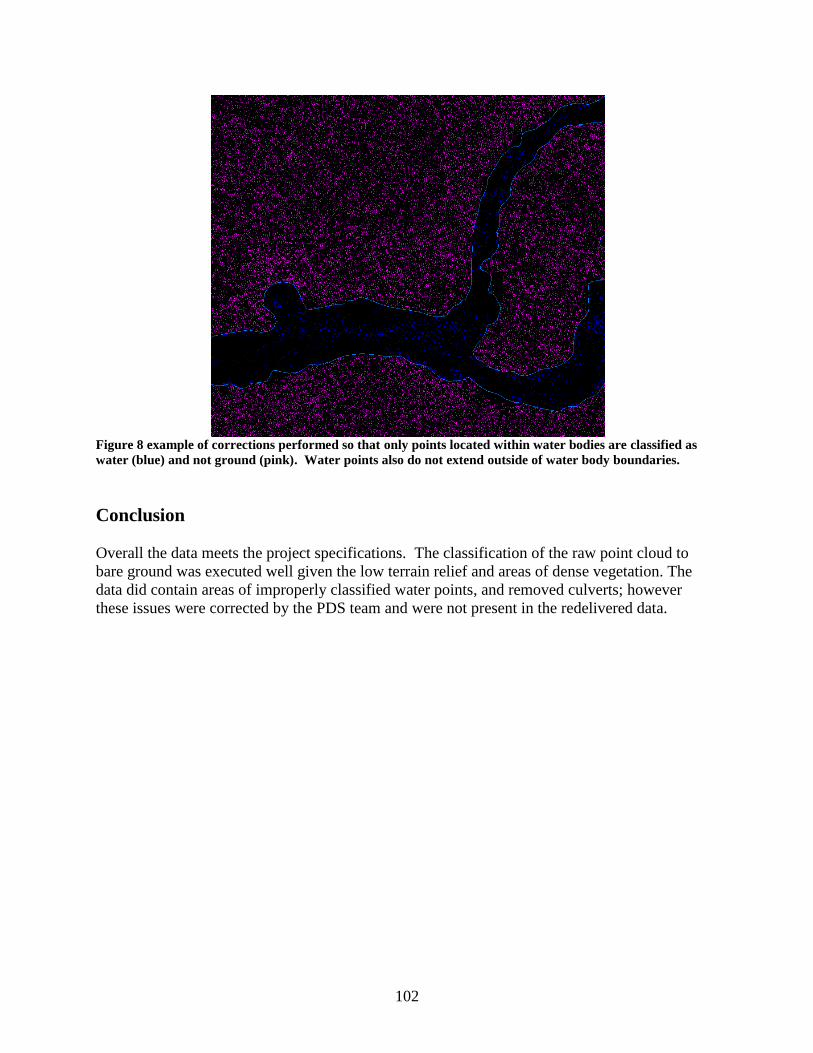
102
Figure 8 example of corrections performed so that only points located within water bodies are classified as
water (blue) and not ground (pink). Water points also do not extend outside of water body boundaries.
Conclusion
Overall the data meets the project specifications. The classification of the raw point cloud to
bare ground was executed well given the low terrain relief and areas of dense vegetation. The
data did contain areas of improperly classified water points, and removed culverts; however
these issues were corrected by the PDS team and were not present in the redelivered data.
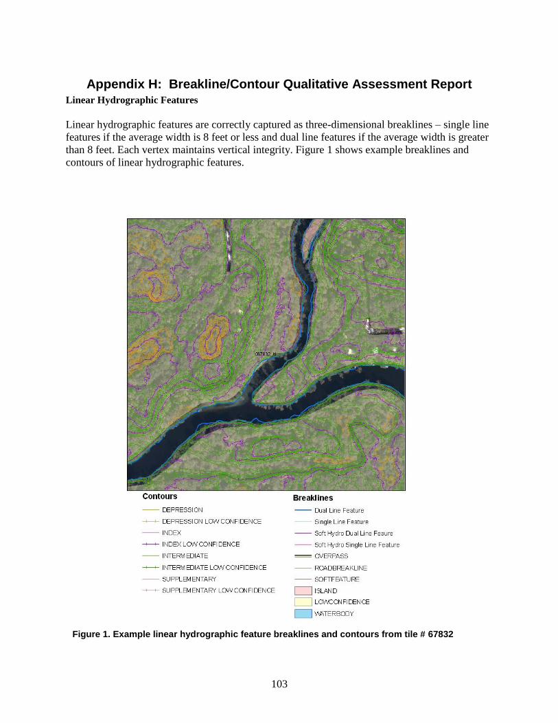
103
Appendix H: Breakline/Contour Qualitative Assessment Report Linear Hydrographic Features
Linear hydrographic features are correctly captured as three-dimensional breaklines – single line
features if the average width is 8 feet or less and dual line features if the average width is greater
than 8 feet. Each vertex maintains vertical integrity. Figure 1 shows example breaklines and
contours of linear hydrographic features.
Figure 1. Example linear hydrographic feature breaklines and contours from tile # 67832
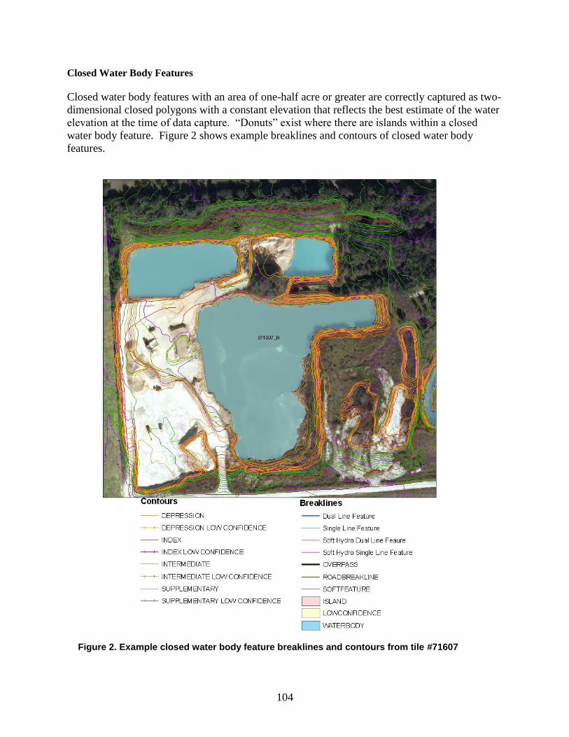
104
Closed Water Body Features
Closed water body features with an area of one-half acre or greater are correctly captured as two-
dimensional closed polygons with a constant elevation that reflects the best estimate of the water
elevation at the time of data capture. “Donuts” exist where there are islands within a closed
water body feature. Figure 2 shows example breaklines and contours of closed water body
features.
Figure 2. Example closed water body feature breaklines and contours from tile #71607
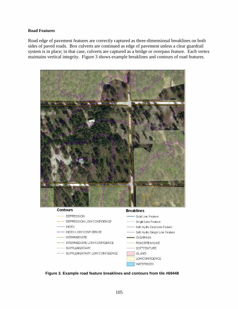
105
Road Features
Road edge of pavement features are correctly captured as three-dimensional breaklines on both
sides of paved roads. Box culverts are continued as edge of pavement unless a clear guardrail
system is in place; in that case, culverts are captured as a bridge or overpass feature. Each vertex
maintains vertical integrity. Figure 3 shows example breaklines and contours of road features.
Figure 3. Example road feature breaklines and contours from tile #69448
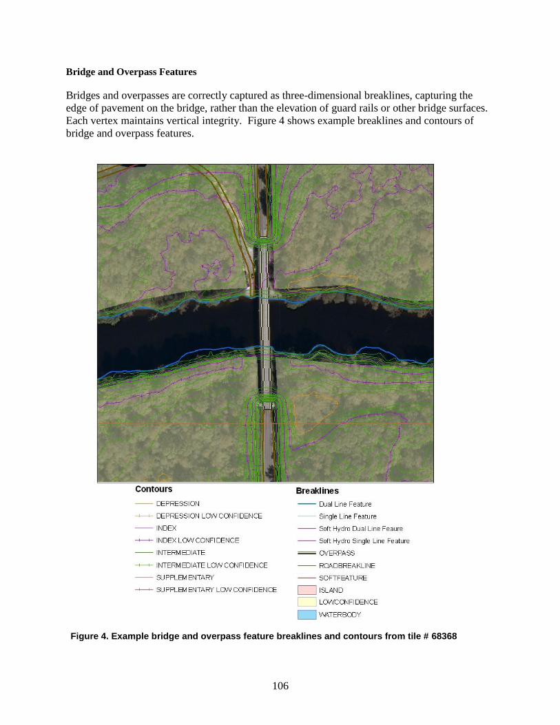
106
Bridge and Overpass Features
Bridges and overpasses are correctly captured as three-dimensional breaklines, capturing the
edge of pavement on the bridge, rather than the elevation of guard rails or other bridge surfaces.
Each vertex maintains vertical integrity. Figure 4 shows example breaklines and contours of
bridge and overpass features.
Figure 4. Example bridge and overpass feature breaklines and contours from tile # 68368
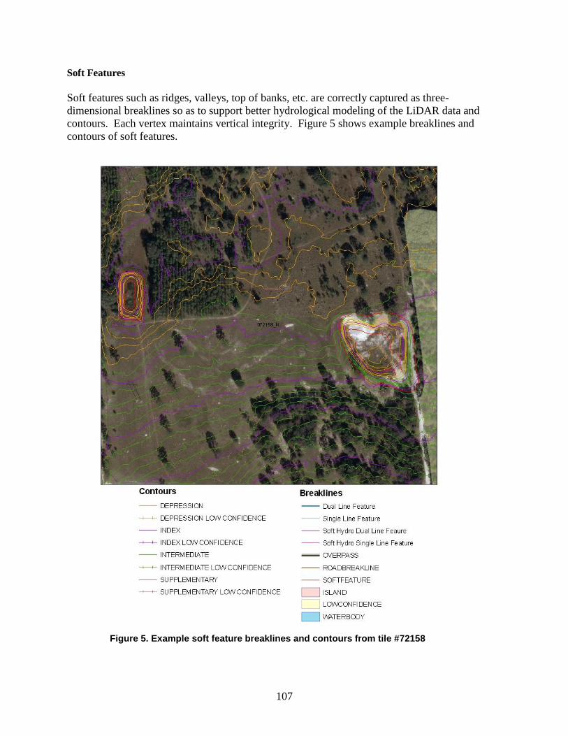
107
Soft Features
Soft features such as ridges, valleys, top of banks, etc. are correctly captured as three-
dimensional breaklines so as to support better hydrological modeling of the LiDAR data and
contours. Each vertex maintains vertical integrity. Figure 5 shows example breaklines and
contours of soft features.
Figure 5. Example soft feature breaklines and contours from tile #72158
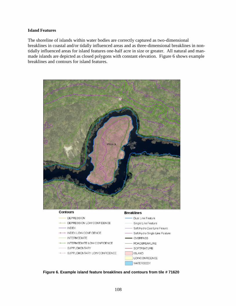
108
Island Features
The shoreline of islands within water bodies are correctly captured as two-dimensional
breaklines in coastal and/or tidally influenced areas and as three-dimensional breaklines in non-
tidally influenced areas for island features one-half acre in size or greater. All natural and man-
made islands are depicted as closed polygons with constant elevation. Figure 6 shows example
breaklines and contours for island features.
Figure 6. Example island feature breaklines and contours from tile # 71620
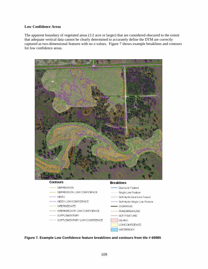
109
Low Confidence Areas
The apparent boundary of vegetated areas (1/2 acre or larger) that are considered obscured to the extent
that adequate vertical data cannot be clearly determined to accurately define the DTM are correctly
captured as two-dimensional features with no z-values. Figure 7 shows example breaklines and contours
for low confidence areas.
Figure 7. Example Low Confidence feature breaklines and contours from tile # 69985
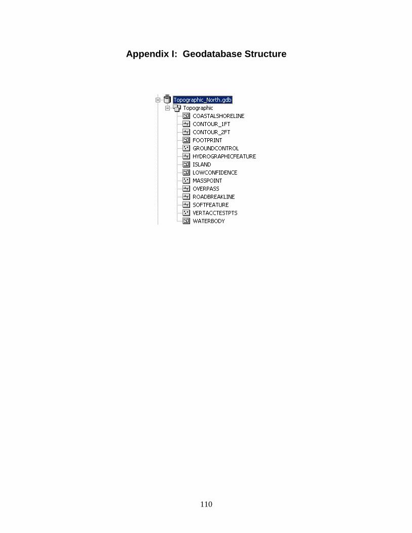
110
Appendix I: Geodatabase Structure