1

Contract # WC133R10CN0212 Project # NRMC0009-10-13054 13-450

Ocean Current Radar Calibration with Ships of Opportunity and the Automatic Identification

System

Phase I Final Report

Brian Emery1, Chad Whelan2, Don Barrick2, and Libe Washburn3

1Marine Science Institute, University of California, Santa Barbara, CA, 93106, U.S.A 2Codar Ocean Sensors, Ltd., Mountain View, CA, 94043, U.S.A

3Department of Geography, University of California, Santa Barbara, CA, 93106, U.S.A

EXECUTIVE SUMMARY

We investigate the feasibility of calibrating HF radar systems using HF backscatter from ships along with Automatic Identification System (AIS) broadcasts. We obtained data from 4 SeaSondes, located in the vicinity of the Santa Barbara Channel, with coincident AIS data recorded over 70 days. Using the ship position information from AIS, we identify corresponding ship echoes in SeaSonde HF radar cross spectra, and use this information to reproduce receive antenna patterns over a wide range of bearings.

We meet the proposed Phase I objectives as follows: 1) When matched with backscattered signal in cross spectra, the ship positions can be used to accurately reproduce the receive antenna pattern as a function of bearing; 2) Results indicate that accurate antenna patterns can be obtained from as few as 8 individual ships, suggesting that proximity to high volume shipping lanes is not essential; 3) The global scope of the AIS system would allow this method to be used on any of the approximately 350 HF radars in operation world-wide, including all of the IOOS national network sites.

The methods presented here are a cost effective way to frequently calibrate HF radar systems. We envision a commercial software product operating on HF radar site computers that integrates data from AIS receivers into the HF radar data processing, producing receive antenna patterns in real time.

This material is based upon work supported by the Department of Commerce under contract number: WC133R10CN0212. Any opinions, findings, conclusions or recommendations expressed in this publication are those of the author(s) and do not necessarily reflect the views of the Department of Commerce.

2

I. INTRODUCTION

Several studies have demonstrated improved ocean current data quality when using measured receive antenna patterns [1], [2] and best practices call for them as a necessary component of the quality assurance and quality control of high frequency (HF) radar data [3]. Additionally, precise, high-resolution antenna calibrations are necessary for successful deployment of emerging bi-static and multi-static HF radar systems. Currently only 41 of the 110 sites reporting data to the NOAA Integrated Ocean Observing System (IOOS) national network use measured patterns [4], primarily because of the expense and inconvenience of measuring patterns with conventional transponder methods. As critical functions such as United States Coast Guard (USCG) Search and Rescue (SAR) operations and NOAA Hazmat spill response become dependent on NOAA IOOS HF radar data, an inexpensive, simple, and robust calibration method is needed to ensure the highest quality data.

Measurement of the receive antenna pattern typically involves a small boat, which can navigate close to shore while carrying a GPS receiver and HF transponder. The boat follows an arc of constant range, generally 500 – 2000 m from the HF radar site. The transponder provides a coherent signal source and the GPS receiver provides the time-stamped positions of the boat. Data obtained at the HF radar site during this process are later combined with the GPS positions of the boat (and transponder) to determine the antenna pattern. Including processing time, about 2 HF radar sites can be calibrated in a day. Weather and sea state must be conducive to operating a small vessel. Costs for technician and boat time are on the order of $1000-$2000 per site per calibration and these may be needed multiple times per year, per site. Consequently, annual calibration of the IOOS national network costs from $100,000 to $500,000.

A common approach to calibrating radars in other bands, such as Over-the-Horizon Radars (OTHR), uses reflective objects with known properties to evaluate the systems. Previous studies have used HF signals backscattered from ships to produce relative phase calibrations of a non-direction finding (DF) phased array receive antenna [5], [6]. Because of hardware differences, this method cannot be used with DF-type systems, such as the CODAR SeaSondes used by most IOOS participants. Furthermore, these studies treated the position of the ships backscattering their signal as an unknown, which is insufficient for a complete calibration. Even for non-DF systems, the lack of an independent position for the vessel results an undesired approximation of the phase calibrations.

Many commercial shipping vessels now broadcast position and other information using the Automatic Information System (AIS). The AIS system, designed and used primarily for collision avoidance and maritime domain awareness, broadcasts every 2-10 s while underway. These broadcasts include ship identification, latitude, longitude, speed, and heading, and are receivable by anyone with the proper equipment and software. The AIS system operates in the maritime VHF band, with a range on the order of 100 km, which is close to the operational range of 12-13 MHz ocean current monitoring HF radars, currently the most numerous radars in the IOOS national network.

3

The Phase I objectives are: 1) Demonstrate the use of backscatter from ships and corresponding AIS position data to reproduce antenna patterns previously measured with a transponder; 2) Determine the relationship between accuracy of the reproduced pattern and the number of AIS observations required to make it. Use this relationship to predict how frequently a pattern can be produced given a known level of ship traffic; 3) Use historical AIS data to estimate the fraction of existing HF radars that could use this technology, and how often they could use it to produce a pattern.

Following the Phase I objectives, we describe the use of AIS data and ship

backscatter to derive receive antenna calibrations for four HF radars located along the Santa Barbara Channel. We demonstrate the success of the method by comparisons with standard antenna calibrations, and then describe a metric for comparing the two methods. We show that very few ships are needed to reproduce antenna patterns, and then we investigate the global availability of AIS data. Finally, we discuss the implications and directions for further research.

II. METHODS

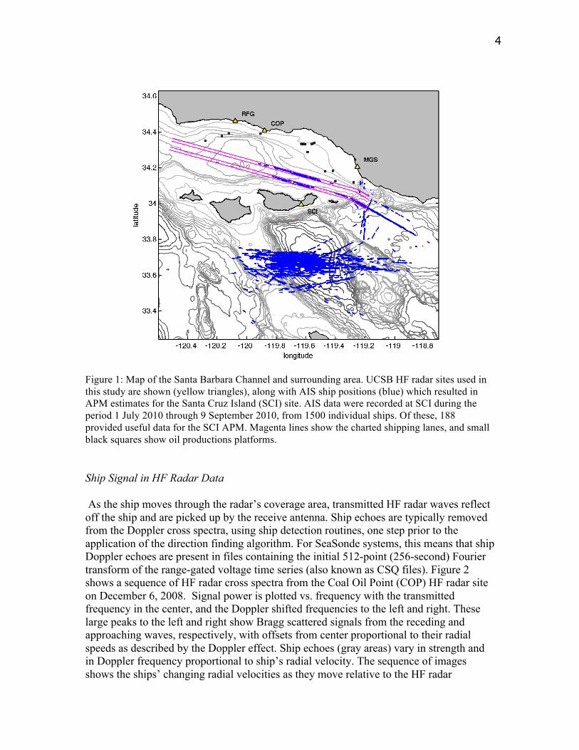
Data were obtained from 4 SeaSonde HF radars operating at 12-13 MHz and located adjacent to shipping routes leading to the major ports of southern California. The radars are owned by University of California, Santa Barbara. The SeaSondes at Refugio State Beach (RFG), Coal Oil Point (COP), the Mandalay Generating Station (MGS) and Santa Cruz Island (SCI) provided echo cross-spectra for the calculation of ship-derived patterns (ASHIP hereafter), and transponder-measured antenna patterns (ATRANS) for validation. Antenna pattern measurements followed the standard method: a small boat carried a signal source along an circular arc to maintain zero radial velocity relative to the radar site, and the arc was traversed twice over a wide range of bearings. Instead of using a transponder, a modified radar transmitter producing a strong signal was used. This allowed the boat to operate at greater ranges, 15 km for SCI and 2.5 km for the other sites. Using these methods, ATRANS were measured at RFG (5 August 2010), MGS (13 August 2010), COP (18 August 2010), and SCI (9 September 2010). Cross spectra containing ship backscatter were obtained from each of the sites spanning 1 July 2010 through 9 September 2010. AIS Ship Data The SCI HF radar site houses an AIS receiver and dedicated computer that records the AIS broadcasts. The resulting log files contain ship speed, heading, latitude, longitude, time and other identifying information. From 1 July 2010 00:00 UTC through 9 September 2010 23:00 UTC (1703 hours) we received AIS data from 1500 individual ships. From the AIS log files we compute range, bearing, and the radial component of the ship velocity relative to each of 4 HF radar sites. Range and radial velocity are then used to identify 1) ships falling within the operating range of the HF site; and 2) ships moving at a non-zero velocity relative to the site. As an example, Figure 1 shows the locations of the 188 ships that provided useful signal for the SCI antenna pattern estimate.

4

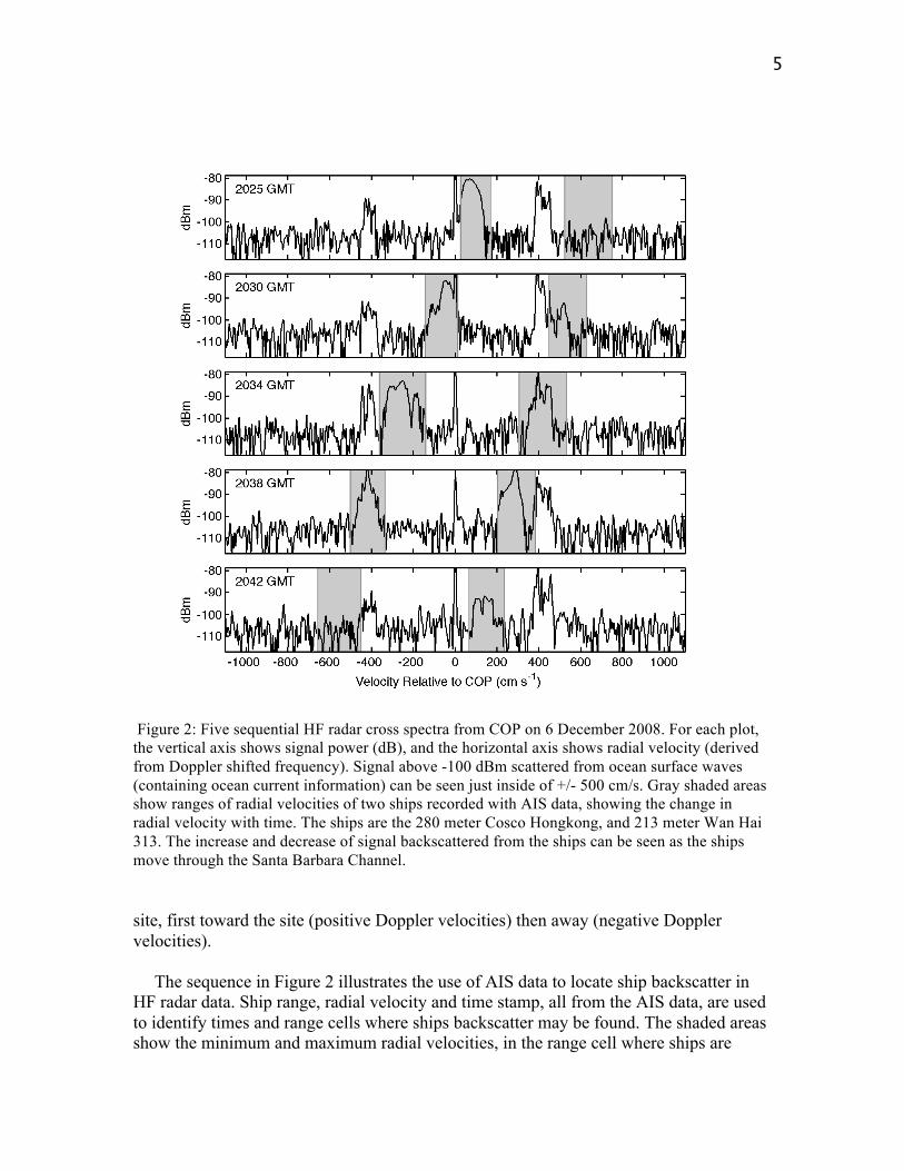
Figure 1: Map of the Santa Barbara Channel and surrounding area. UCSB HF radar sites used in this study are shown (yellow triangles), along with AIS ship positions (blue) which resulted in APM estimates for the Santa Cruz Island (SCI) site. AIS data were recorded at SCI during the period 1 July 2010 through 9 September 2010, from 1500 individual ships. Of these, 188 provided useful data for the SCI APM. Magenta lines show the charted shipping lanes, and small black squares show oil productions platforms. Ship Signal in HF Radar Data As the ship moves through the radar’s coverage area, transmitted HF radar waves reflect off the ship and are picked up by the receive antenna. Ship echoes are typically removed from the Doppler cross spectra, using ship detection routines, one step prior to the application of the direction finding algorithm. For SeaSonde systems, this means that ship Doppler echoes are present in files containing the initial 512-point (256-second) Fourier transform of the range-gated voltage time series (also known as CSQ files). Figure 2 shows a sequence of HF radar cross spectra from the Coal Oil Point (COP) HF radar site on December 6, 2008. Signal power is plotted vs. frequency with the transmitted frequency in the center, and the Doppler shifted frequencies to the left and right. These large peaks to the left and right show Bragg scattered signals from the receding and approaching waves, respectively, with offsets from center proportional to their radial speeds as described by the Doppler effect. Ship echoes (gray areas) vary in strength and in Doppler frequency proportional to ship’s radial velocity. The sequence of images shows the ships’ changing radial velocities as they move relative to the HF radar

5

Figure 2: Five sequential HF radar cross spectra from COP on 6 December 2008. For each plot, the vertical axis shows signal power (dB), and the horizontal axis shows radial velocity (derived from Doppler shifted frequency). Signal above -100 dBm scattered from ocean surface waves (containing ocean current information) can be seen just inside of +/- 500 cm/s. Gray shaded areas show ranges of radial velocities of two ships recorded with AIS data, showing the change in radial velocity with time. The ships are the 280 meter Cosco Hongkong, and 213 meter Wan Hai 313. The increase and decrease of signal backscattered from the ships can be seen as the ships move through the Santa Barbara Channel.

site, first toward the site (positive Doppler velocities) then away (negative Doppler velocities).

The sequence in Figure 2 illustrates the use of AIS data to locate ship backscatter in

HF radar data. Ship range, radial velocity and time stamp, all from the AIS data, are used to identify times and range cells where ships backscatter may be found. The shaded areas show the minimum and maximum radial velocities, in the range cell where ships are

6

located, as determined from AIS data. The widths of the gray areas illustrate the significant variation in the ships’ radial velocities during each 256 s interval. Some of this variability results from changes in radial velocity as the ships move relative to the site and some variability may be due to ship roll. The variability in the radial velocity causes the ship backscatter signal to spread in a broad peak across several frequency bins. Variability in auto spectral amplitude as the ships move through the radar coverage area can also be seen.

When using the ship backscatter for antenna pattern processing, regions around zero

Doppler, and near the Bragg region are excluded because the ship signal mixes with other known, strong backscattered signals (such as the ocean surface currents). Further steps below apply to all frequency bins identified with the AIS data.

Antenna Pattern Measurements (APMs)

After identifying coincident ship echo and AIS data, the next step is to use this signal to determine the receive antenna pattern at the ship’s bearing. Determination of the receive antenna pattern follows from the MUSIC algorithm as it is applied to extract ocean current data [6]. In the ocean current case, the radial velocity and antenna pattern are known, and are used to determine bearing. In the case presented here, a signal source (i.e. echo from an AIS ship) with a known bearing and radial velocity are used to determine the antenna pattern.

As outlined [6], we begin with the voltage time series of the 3 receive antennas (1

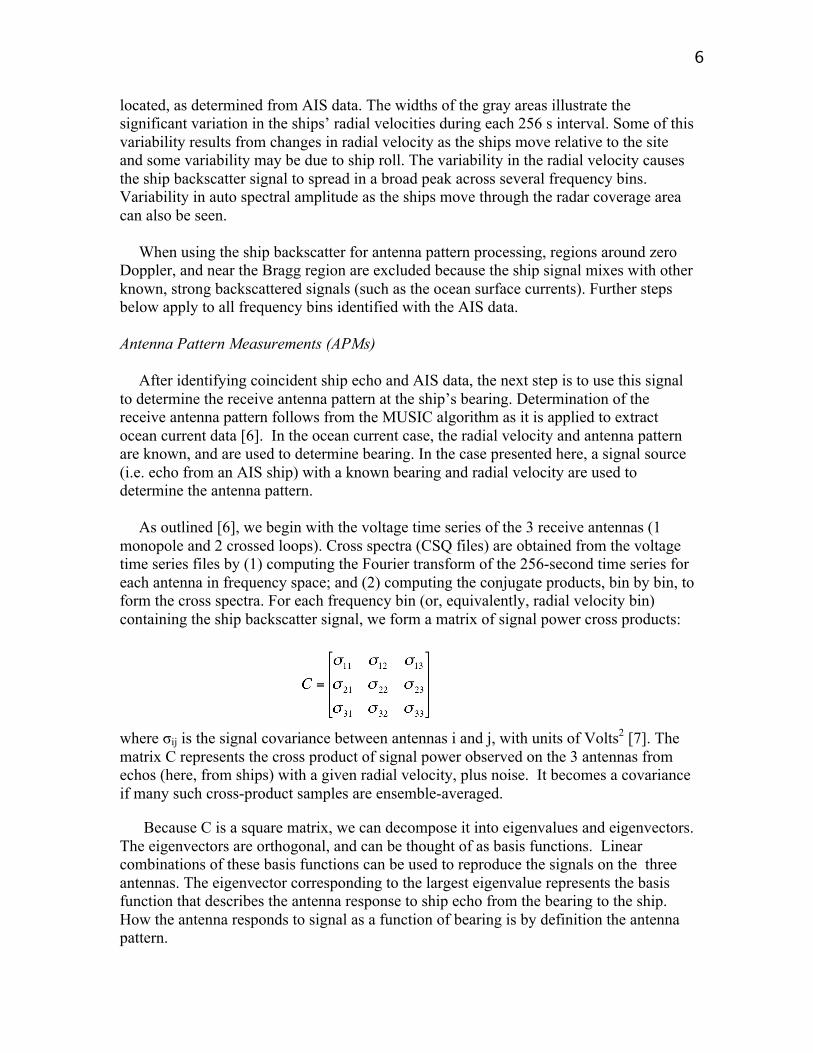
monopole and 2 crossed loops). Cross spectra (CSQ files) are obtained from the voltage time series files by (1) computing the Fourier transform of the 256-second time series for each antenna in frequency space; and (2) computing the conjugate products, bin by bin, to form the cross spectra. For each frequency bin (or, equivalently, radial velocity bin) containing the ship backscatter signal, we form a matrix of signal power cross products:

where σij is the signal covariance between antennas i and j, with units of Volts2 [7]. The matrix C represents the cross product of signal power observed on the 3 antennas from echos (here, from ships) with a given radial velocity, plus noise. It becomes a covariance if many such cross-product samples are ensemble-averaged.

Because C is a square matrix, we can decompose it into eigenvalues and eigenvectors. The eigenvectors are orthogonal, and can be thought of as basis functions. Linear combinations of these basis functions can be used to reproduce the signals on the three antennas. The eigenvector corresponding to the largest eigenvalue represents the basis function that describes the antenna response to ship echo from the bearing to the ship. How the antenna responds to signal as a function of bearing is by definition the antenna pattern.

7

For determining bearing to ocean currents, we would exploit the orthogonality of the

eigenvectors and compare the noise eigenvectors to the measured antenna pattern to find the bearing at which the vector dot product approaches zero. The bearing where the antenna pattern is most orthogonal to the noise eigenvectors is the bearing to the signal source. For determining antenna patterns, the bearing of the source is known (from AIS) and the signal eigenvector contains the estimate of the antenna pattern at the AIS bearing.

For a given ship and CSQ file, several estimates of the antenna pattern over a range of

bearings are obtained, since the ship signal spans several spectral frequency bins. Storing the antenna pattern estimates along with the ship size (included in the AIS data), the signal-to-noise ratio (SNR) on each of the 3 receive antennas, and statistics of the AIS ship radial velocities during the cross spectra processing time (i.e. for each CSQ file), allows for the application of various smoothing and filtering techniques in the next step.

Averaging/smoothing of the antenna pattern estimates

Large variations occur in the initial ASHIP estimate likely result from variations in the backscattered signals on the three antennas due to commonly seen echo strength fluctuations. Estimates stabilize when limiting the ship length to > 100 m, the standard deviation of ship radial velocities to < 25 cm/s, and the SNR > 15 dB. Further improvements are obtained by bin-averaging APMs over 5 degrees. Results from individual ships suggest that larger ships produce ASHIP estimates which more closely match ATRANS.. Large radial velocity standard deviations are excluded to limit ships to those with a constant and favorable direction of travel. Limiting radial velocity standard deviations also minimizes the effect of ship roll, which may alter echo amplitudes, spread spectral peaks, and generally degrade ASHIP estimates. Limiting SNR to above 15 dB assures a strong enough signal to separate from the background noise.

We compute 95% confidence intervals for the ASHIP estimates after bin averaging as a function of bearing. The confidence intervals on the bin mean (X) are computed as a function of the standard deviation (std) and the degrees of freedom (Nd), using the following formula:

X ± t*( std/sqrt(Nd) ) Here t is computed from the inverse of Student's T cumulative distribution function, given the desired probability (95% gives us an alpha = (1-0.95)/2 = 0.0250) and Nd. Note that the Student's T distribution approaches the normal distribution for large Nd, and becomes 1.96 for Nd greater than about 20.

Since adjacent points within a given cross spectra ship peak are not completely

independent, degrees of freedom are conservatively estimated by counting the number of ships returning data per cross spectra. For example, one ship peak in one CSQ file may give us 5 estimates of the antenna pattern at a particular bearing, but for the purpose of

8

computing the confidence interval, this is counted as 1 degree of freedom. This method likely produces a lower bound on the degrees of freedom, and thus wider, more conservative confidence intervals. Comparison Metrics

As described above, the antenna pattern at a given bearing is a four-element complex vector, consisting of the real and imaginary components of each of the two loop antennas. (The real and imaginary components can alternatively be expressed as magnitude and phase). For example, at each bearing, the pattern is expressed as,

A(θ) = [ A13R(θ) A13I(θ) A23R(θ) A23I(θ) ] where A13R denotes the loop 1 real component, A13I denotes the loop 1 imaginary component, and similarly for loop 2. Each component is normalized by the monopole (antenna 3). To simplify comparisons of ASHIP with ATRANS we use a quality metric based on the MUSIC direction of arrival calculation [11]. The inverse distance between two points in space at a given bearing θ is defined:

D(θ)-1 = 10*log10( ( conj(ASHIP(θ) - ATRANS(θ))T(ASHIP(θ) - ATRANS(θ)) )-1/2 ) Geometrically, this is the inverse of the Euclidean distance between two points in space. In this application, the locations of the two points are described with a 4 dimensional complex space, with the log transform converting units to dB. Described previously [10] as a metric representing the quality of bearings obtained with MUSIC, we use this quantity to summarize the similarity of two antenna patterns at a given bearing. As demonstrated below, higher values of D-1 indicate better agreement.

III. RESULTS

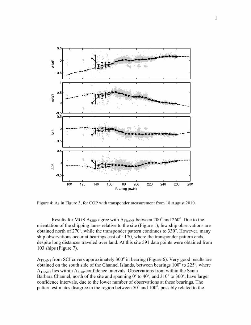
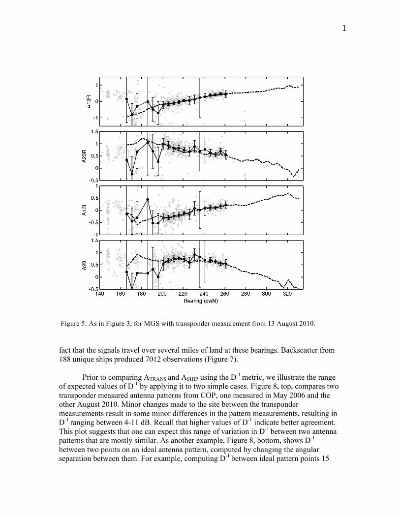
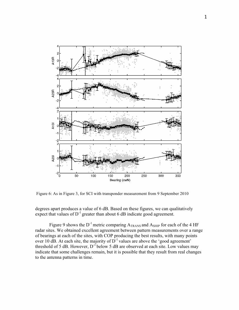
Figures 3, 4, 5 and 6 show antenna patterns ATRANS, and ASHIP for RFG, COP, MGS, and SCI respectively. ATRANS (dashed lines) were measured previously with a boat and transponder, with ASHIP estimates from individual ships shown as gray dots. Bin averaged ASHIP (black dots and solid lines) with 95% confidence intervals are also shown at 5o increments.

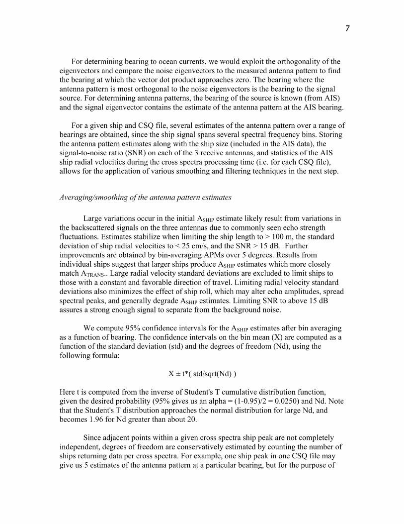
Results from RFG are shown in Figure 3. Some differences are observed but the

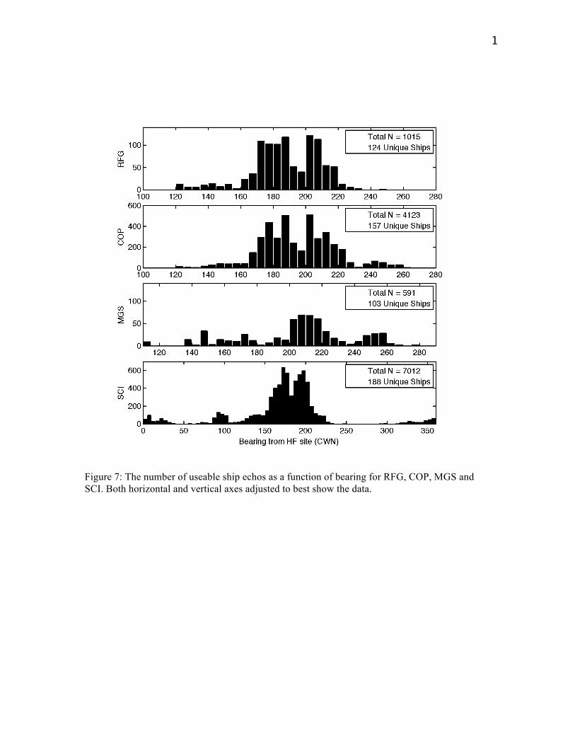
overall shape of the pattern is reproduced with the ATRANS falling within 95% confidence intervals of ASHIP at most bearings. At RFG, ATRANS extends over bearings from 90o to 275o, while ASHIP extends from 125o to 225o. Some disagreement occurs between 180o and 200o in the imaginary components of both loops due to data points near -1. Backscattered signal from 124 ships resulted in 1015 observations, with the distribution as a function of bearing shown in Figure 7.

9

Figure 3: RFG antenna pattern components (top to bottom: Loop 1 real, Loop2 real, Loop1 imaginary, Loop2 imaginary). Dashed lines show transponder pattern measured 5 August 2010, gray dots show pattern estimates from individual AIS ships, and large black dots show 5o bin averages of the ship estimates with 95% confidence intervals. AIS and HF radar data are from the period 1 July 2010 through 9 September 2010. Note that in each plot the vertical axes were adjusted to best show the data.

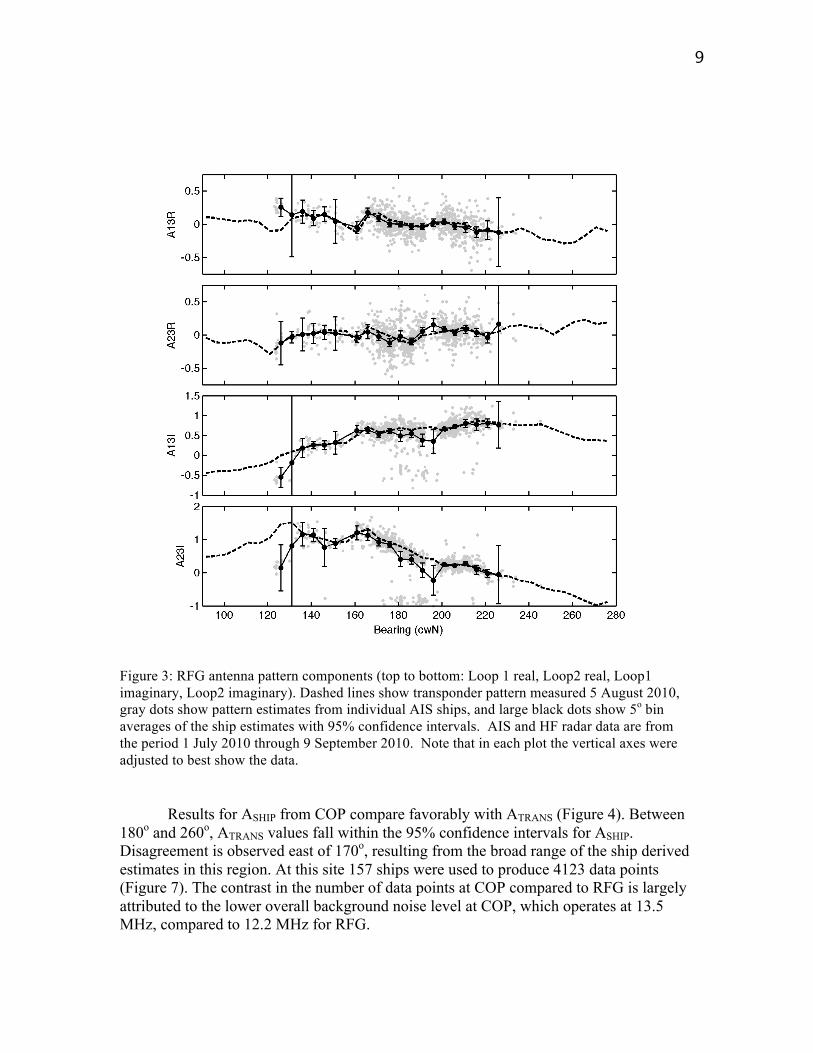
Results for ASHIP from COP compare favorably with ATRANS (Figure 4). Between 180o and 260o, ATRANS values fall within the 95% confidence intervals for ASHIP. Disagreement is observed east of 170o, resulting from the broad range of the ship derived estimates in this region. At this site 157 ships were used to produce 4123 data points (Figure 7). The contrast in the number of data points at COP compared to RFG is largely attributed to the lower overall background noise level at COP, which operates at 13.5 MHz, compared to 12.2 MHz for RFG.

10

Figure 4: As in Figure 3, for COP with transponder measurement from 18 August 2010.

Results for MGS ASHIP agree with ATRANS between 200o and 260o. Due to the orientation of the shipping lanes relative to the site (Figure 1), few ship observations are obtained north of 270o, while the transponder pattern continues to 330o. However, many ship observations occur at bearings east of ~170, where the transponder pattern ends, despite long distances traveled over land. At this site 591 data points were obtained from 103 ships (Figure 7).

ATRANS from SCI covers approximately 300o in bearing (Figure 6). Very good results are obtained on the south side of the Channel Islands, between bearings 100o to 225o, where ATRANS lies within ASHIP confidence intervals. Observations from within the Santa Barbara Channel, north of the site and spanning 0o to 40o, and 310o to 360o, have larger confidence intervals, due to the lower number of observations at these bearings. The pattern estimates disagree in the region between 50o and 100o, possibly related to the

11

Figure 5: As in Figure 3, for MGS with transponder measurement from 13 August 2010. fact that the signals travel over several miles of land at these bearings. Backscatter from 188 unique ships produced 7012 observations (Figure 7).

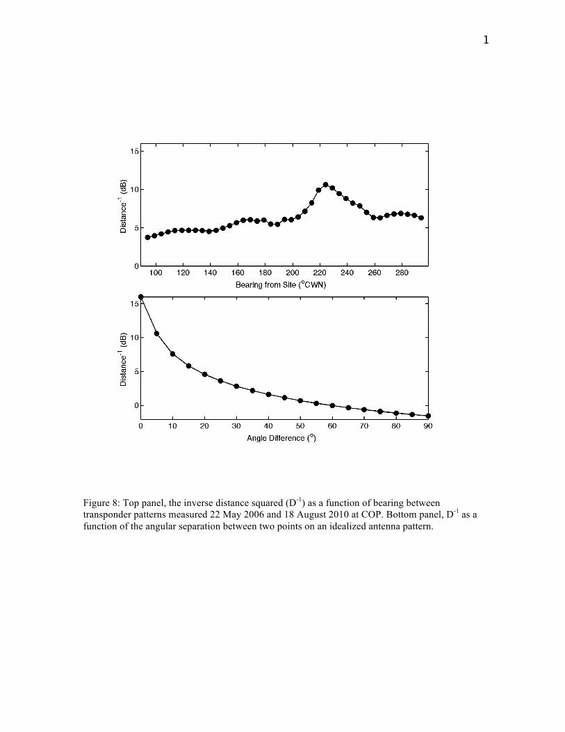
Prior to comparing ATRANS and ASHIP using the D-1 metric, we illustrate the range of expected values of D-1 by applying it to two simple cases. Figure 8, top, compares two transponder measured antenna patterns from COP, one measured in May 2006 and the other August 2010. Minor changes made to the site between the transponder measurements result in some minor differences in the pattern measurements, resulting in D-1 ranging between 4-11 dB. Recall that higher values of D-1 indicate better agreement. This plot suggests that one can expect this range of variation in D-1 between two antenna patterns that are mostly similar. As another example, Figure 8, bottom, shows D-1

between two points on an ideal antenna pattern, computed by changing the angular separation between them. For example, computing D-1 between ideal pattern points 15

12

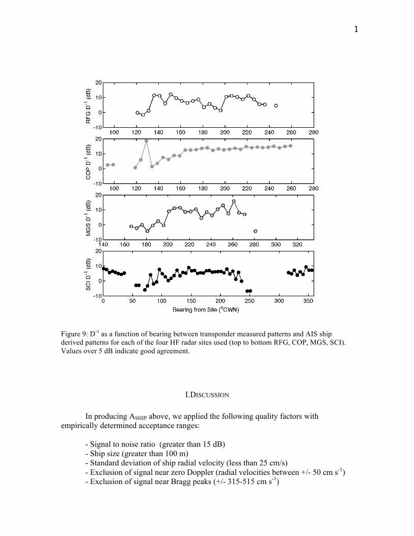
Figure 6: As in Figure 3, for SCI with transponder measurement from 9 September 2010 degrees apart produces a value of 6 dB. Based on these figures, we can qualitatively expect that values of D-1 greater than about 6 dB indicate good agreement. Figure 9 shows the D-1 metric comparing ATRANS and ASHIP for each of the 4 HF radar sites. We obtained excellent agreement between pattern measurements over a range of bearings at each of the sites, with COP producing the best results, with many points over 10 dB. At each site, the majority of D-1 values are above the ‘good agreement’ threshold of 5 dB. However, D-1 below 5 dB are observed at each site. Low values may indicate that some challenges remain, but it is possible that they result from real changes to the antenna patterns in time.

13

Figure 7: The number of useable ship echos as a function of bearing for RFG, COP, MGS and SCI. Both horizontal and vertical axes adjusted to best show the data.

14

Figure 8: Top panel, the inverse distance squared (D-1) as a function of bearing between transponder patterns measured 22 May 2006 and 18 August 2010 at COP. Bottom panel, D-1 as a function of the angular separation between two points on an idealized antenna pattern.

15

Figure 9: D-1 as a function of bearing between transponder measured patterns and AIS ship derived patterns for each of the four HF radar sites used (top to bottom RFG, COP, MGS, SCI). Values over 5 dB indicate good agreement.

I. DISCUSSION

In producing ASHIP above, we applied the following quality factors with empirically determined acceptance ranges: - Signal to noise ratio (greater than 15 dB) - Ship size (greater than 100 m) - Standard deviation of ship radial velocity (less than 25 cm/s) - Exclusion of signal near zero Doppler (radial velocities between +/- 50 cm s-1) - Exclusion of signal near Bragg peaks (+/- 315-515 cm s-1)

16

Surface current extraction is possible with signal to noise ratios (SNR) as low as 7 dB, suggesting that ship backscatter signal with similar SNR may be useable. The choice of ship size distinguishes cargo and tanker ships from barges and tugs, and tended to correlate with ships steaming at a constant rate along a uniform path. An important length scale is the wavelength of the HF radar transmissions, and we suspect that larger ships are likely to provide higher quality backscatter. Limiting the standard deviation of radial velocity screens out ships with too much variation, either in position or speed, during the 256 second cross spectra file. Excluding signal near zero Doppler and in the Bragg scatter zones removed the possibility of interpreting ocean wave signal and other non-ship signal as ship backscatter.

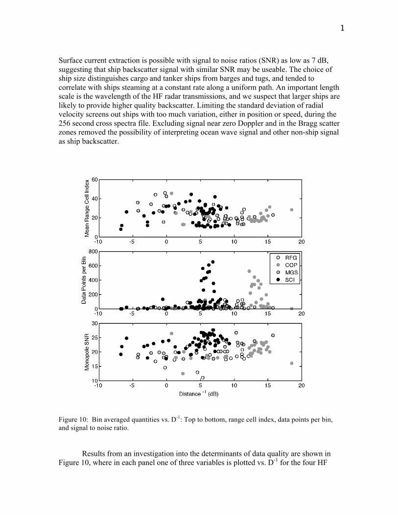
Figure 10: Bin averaged quantities vs. D-1: Top to bottom, range cell index, data points per bin, and signal to noise ratio.

Results from an investigation into the determinants of data quality are shown in Figure 10, where in each panel one of three variables is plotted vs. D-1 for the four HF

17

radar sites. The top panel shows range cell index (effectively, range from the radar site to the ship since range cells are 1.5 km in radial width) vs. the D-1 metric. The middle panel shows data points per bin vs. D-1 and the bottom panel shows signal to noise ratio vs. D-1. The top panel suggests that the best ASHIP data come from range cells 10-30 (15-45 km from the radar site), but otherwise indicates no definitive relationship. An important result of this analysis, shown by the middle panel, is that high quality ASHIP data can come from as few as 20 ship observations per bin (8 unique ship-cross-spectra combinations), meaning that antenna patterns may be computed from ships for HF radar sites in regions with much lower volumes of shipping traffic than were observed here. Little relation with SNR is observed (bottom panel), suggesting that the 15 dB criteria could be relaxed.

In future investigations, we will work to resolve discrepancies between ATRANS

and ASHIP observed at some bearings. For example, some narrow 95% confidence limits for ASHIP do not encompass ATRANS, such as in Figure 3, bottom panel, between 180o and 200o. We speculate this results from estimating APMs at bearings using spectral peaks with large spectral components from non-ship sources such as waves. Future work will improve algorithms to distinguish ship backscatter from these other signals. One approach we will try is to incorporate wave height algorithms to identify second order spectra. Perhaps incorporation of existing ship-removal logic will assist in separating ship echoes from the background second order sea echo, and this will be investigated in subsequent analyses. Some variation in the antenna patterns in time is likely, and future work is needed to establish the normal range and timescales over which changes occur.

Angular coverage of ASHIP in the Santa Barbara channel is strongly influenced by the orientation of the shipping lanes relative to the HF radar sites. Although this analysis focused on backscatter from larger ships, many smaller ships were observed with the AIS broadcasts in regions outside the shipping lanes. With better algorithms for identifying usable backscatter from small ships, it may be possible to obtain estimates of ASHIP over a greater range of bearings.

The characteristics of vessel traffic around other HF radar sites will vary with proximity and orientation to ports and shipping lanes. The distribution and density of vessels near the Santa Barbara HF radar sites may be quite different from that at other sites. In order to investigate these differences, we analyzed AIS data near four HF radar sites, using publicly available data from the website MarineTraffic.com.

Figure 11 shows histograms of the number of vessels per five degrees of azimuth for the following four HF radar sites:

(a) Bodega Marine Lab: 12 MHz (Mid-Range) in Northern California (b) Singing River Island: 5 MHz (Long Range) in Southern Mississippi (c) Holmen Grå: 12 MHz (Mid Range) near Bergen, Norway (d) Sorrento: 25 MHz (Hi-Res) near Napoli, Italy

18

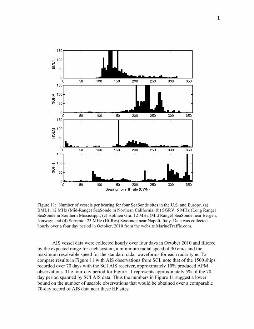
Figure 11: Number of vessels per bearing for four SeaSonde sites in the U.S. and Europe. (a) BML1: 12 MHz (Mid-Range) SeaSonde in Northern California; (b) SGRV: 5 MHz (Long Range) SeaSonde in Southern Mississippi; (c) Holmen Grå: 12 MHz (Mid Range) SeaSonde near Bergen, Norway; and (d) Sorrento: 25 MHz (Hi-Res) Seasonde near Napoli, Italy. Data was collected hourly over a four day period in October, 2010 from the website MarineTraffic.com.

AIS vessel data were collected hourly over four days in October 2010 and filtered by the expected range for each system, a minimum radial speed of 30 cm/s and the maximum resolvable speed for the standard radar waveforms for each radar type. To compare results in Figure 11 with AIS observations from SCI, note that of the 1500 ships recorded over 70 days with the SCI AIS receiver, approximately 10% produced APM observations. The four-day period for Figure 11 represents approximately 5% of the 70 day period spanned by SCI AIS data. Thus the numbers in Figure 11 suggest a lower bound on the number of useable observations that would be obtained over a comparable 70-day record of AIS data near these HF sites.

19

The results in Figure 11 show similar numbers as the distributions for the MGS and RFG HF radars (Figure 7), for which we were able to produce antenna patterns over a majority of bearings (Figures 3, 5). In all of the Figure 11 distributions, however, there is evidence that there will be fewer ships at certain bearings. For instance, at Singing River Island (SGRV), the antenna pattern covers from approximately 100° to 220°, but bearings less than 135° have few ships. The Holmen Grå (HOLM) site measures currents over 360° in early range cells, but primarily measures between 170° and 350° T. HOLM has bearings less than 135° that contained no vessels and some bearings with minimal solutions around 240° and 320° T. These types of gaps appear to be evident at all locations, whether in areas of low or high vessel traffic. Longer time series of AIS may contain AIS broadcasts from smaller ships in these sparse regions, such as was observed in the Santa Barbara Channel. As we suggest above, with better algorithms for identifying usable backscatter from small ships, it may be possible to obtain antenna pattern estimates at bearings with minimal shipping traffic.

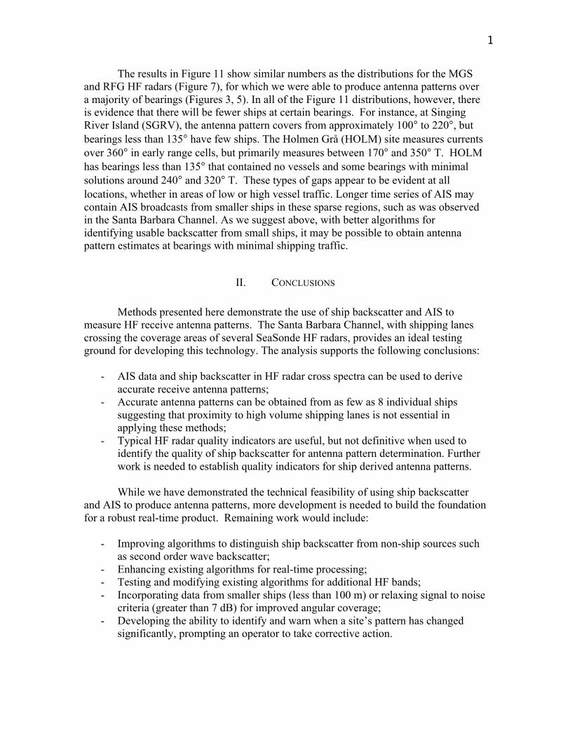
II. CONCLUSIONS

Methods presented here demonstrate the use of ship backscatter and AIS to measure HF receive antenna patterns. The Santa Barbara Channel, with shipping lanes crossing the coverage areas of several SeaSonde HF radars, provides an ideal testing ground for developing this technology. The analysis supports the following conclusions:

- AIS data and ship backscatter in HF radar cross spectra can be used to derive accurate receive antenna patterns;

- Accurate antenna patterns can be obtained from as few as 8 individual ships suggesting that proximity to high volume shipping lanes is not essential in applying these methods;

- Typical HF radar quality indicators are useful, but not definitive when used to identify the quality of ship backscatter for antenna pattern determination. Further work is needed to establish quality indicators for ship derived antenna patterns.

While we have demonstrated the technical feasibility of using ship backscatter

and AIS to produce antenna patterns, more development is needed to build the foundation for a robust real-time product. Remaining work would include:

- Improving algorithms to distinguish ship backscatter from non-ship sources such as second order wave backscatter;

- Enhancing existing algorithms for real-time processing; - Testing and modifying existing algorithms for additional HF bands; - Incorporating data from smaller ships (less than 100 m) or relaxing signal to noise

criteria (greater than 7 dB) for improved angular coverage; - Developing the ability to identify and warn when a site’s pattern has changed

significantly, prompting an operator to take corrective action.

20

Given the ubiquity of shipping in coastal waters, the global use of AIS broadcasting, and the identified need for more frequent antenna pattern measurements, the method presented here could significantly improve the quality of ocean current data from the existing global HF radar network and at much lower cost than traditional methods. In addition to the cost savings of measuring antenna patterns, increased quality of HF radar data across the entire IOOS network itself has an inherent value for spill response, search and rescue, and other operational uses.

ACKNOWLEDGMENT We thank Megan McKenna (Scripps Institution of Oceanography) for use of the AIS data.

REFERENCES

[1] Paduan, J. D., K. C. Kim, M. S. Cook, and F. P Chavez, 2006. Calibration and Validation of Direction-Finding High-Frequency Radar Ocean Surface Current Observations, IEEE J. of Oceanic Engineering, vol. 31, no. 4, DOI 10.1109/JOE.2006.886195

[2] Kohut, J. T. and S. M. Glenn, 2003. Calibration of HF radar surface current measurements using measured antenna beam patterns. J. Atmos. Ocean. Tech., 1303-1316.

[3] SCCOOS Best Practices Document (based on Radio-wave Operators Working Group meetings (ROWG)):http://cordc.ucsd.edu/projects/mapping/documents/SCCOOS-BestPractices.pdf

[4] HFR Network system calibrations (idealized or measured): http://www.sccoos.org/data/hfrnet/xml/stationStatus.php

[5] Fernandez, D. M., J. F. Vesecky, and C. C. Teague, 2003, Calibration of HF radar systems with ships of opportunity, Proc. Intl. Geosci. Remote Sens. Symp. (IGARSS), vol. 7, pp 4271-3.

[6] Fernandez, D. M., J. F. Vesecky, and C. C. Teague, (2006) Phase corrections of small-loop HF radar system receive arrays with ships of opportunity, IEEE J. of Oceanic Engineering, vol. 31, no. 4, DOI 10.1109/JOE.2006.886238

[7] D. E. Barrick, and B. J. Lipa (1999), Radar angle determination with MUSIC direction finding, U. S. Patent 5,990,834.

[8] Lipa, B.J. and D.E. Barrick (1983), Least-squares methods for the extraction of surface currents from CODAR crossed-loop data: Application at ARSLOE, IEEE J. Oceanic Engr., vol. OE-8, pp. 226-253.

21

[8] Barrick, D. E. and B. J. Lipa (1997), Evolution of bearing determination in HF current mapping radars, Oceanography, vol. 10, no. 2, pp. 72-75.

[9] Barrick, D.E., Lipa, B.J. (1999), Using antenna patterns to improve the quality of SeaSonde HF radar surface current maps, Proceedings of the IEEE Sixth Working Conference on Current Measurement, pp. 5-8, DOI 10.1109/CCM.1999.755204.

[10] de Paolo, T.; Cook, T.; Terrill, E.; , "Properties of HF RADAR Compact Antenna Arrays and Their Effect on the MUSIC Algorithm," OCEANS 2007 , vol., no., pp.1-10, Sept. 29 2007-Oct. 4 2007, doi: 10.1109/OCEANS.2007.4449265

[11] Schmidt, R. O., 1986: Multiple emitter location and signal parameter estimation. IEEE Trans. Antennas Propag., 34, 276–280.