Final Review

Dr. Bernard Chen Ph.D.University of Central Arkansas

Spring 2010

Outline

Hash Table Recursion Sorting

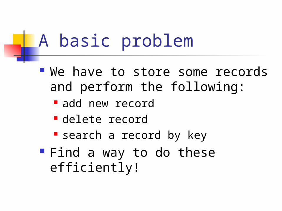
A basic problem

We have to store some records and perform the following: add new record delete record search a record by key

Find a way to do these efficiently!

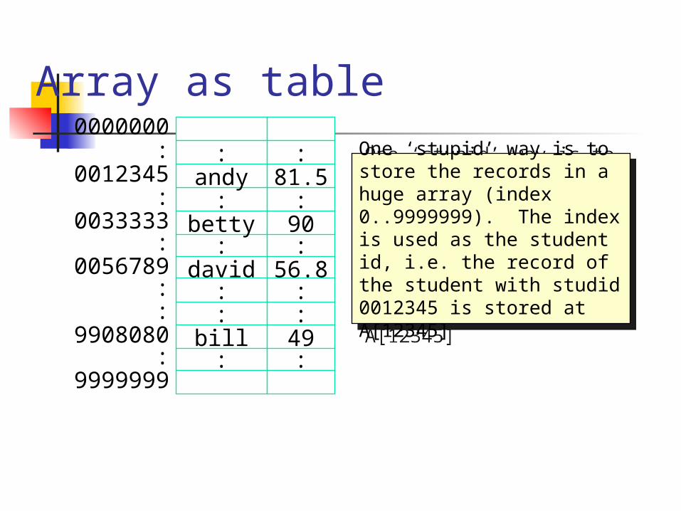
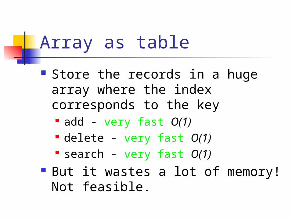
Array as table

:0033333

:0012345

0000000:

:betty

:andy

:

:90:

81.5:

name score

0056789 david 56.8

:9908080

::

:bill::

:49::

9999999

One ‘stupid’ way is to store the records in a huge array (index 0..9999999). The index is used as the student id, i.e. the record of the student with studid 0012345 is stored at A[12345]

One ‘stupid’ way is to store the records in a huge array (index 0..9999999). The index is used as the student id, i.e. the record of the student with studid 0012345 is stored at A[12345]

Array as table

Store the records in a huge array where the index corresponds to the key add - very fast O(1) delete - very fast O(1) search - very fast O(1)

But it wastes a lot of memory! Not feasible.

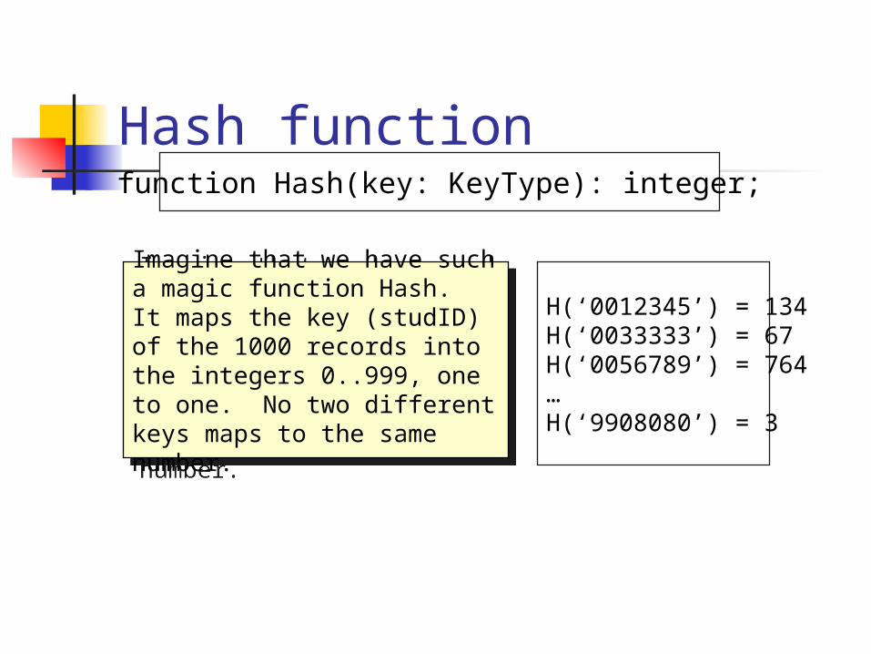
Hash functionfunction Hash(key: KeyType): integer;

Imagine that we have such a magic function Hash. It maps the key (studID) of the 1000 records into the integers 0..999, one to one. No two different keys maps to the same number.

Imagine that we have such a magic function Hash. It maps the key (studID) of the 1000 records into the integers 0..999, one to one. No two different keys maps to the same number.

H(‘0012345’) = 134H(‘0033333’) = 67H(‘0056789’) = 764…H(‘9908080’) = 3

Hash Table

:betty

:bill:

:90:

49:

name score

andy 81.5

::

david:

::

56.8:

:0033333

:9908080

:

0012345

::

0056789:

3

67

0

764

999

134

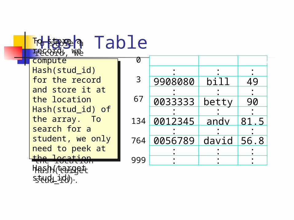
To store a record, we compute Hash(stud_id) for the record and store it at the location Hash(stud_id) of the array. To search for a student, we only need to peek at the location Hash(target stud_id).

To store a record, we compute Hash(stud_id) for the record and store it at the location Hash(stud_id) of the array. To search for a student, we only need to peek at the location Hash(target stud_id).

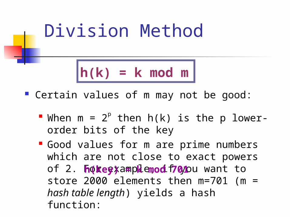
Division Method

Certain values of m may not be good:

When m = 2p then h(k) is the p lower-order bits of the key

Good values for m are prime numbers which are not close to exact powers of 2. For example, if you want to store 2000 elements then m=701 (m = hash table length) yields a hash function:

h(k) = k mod m

h(key) = k mod 701

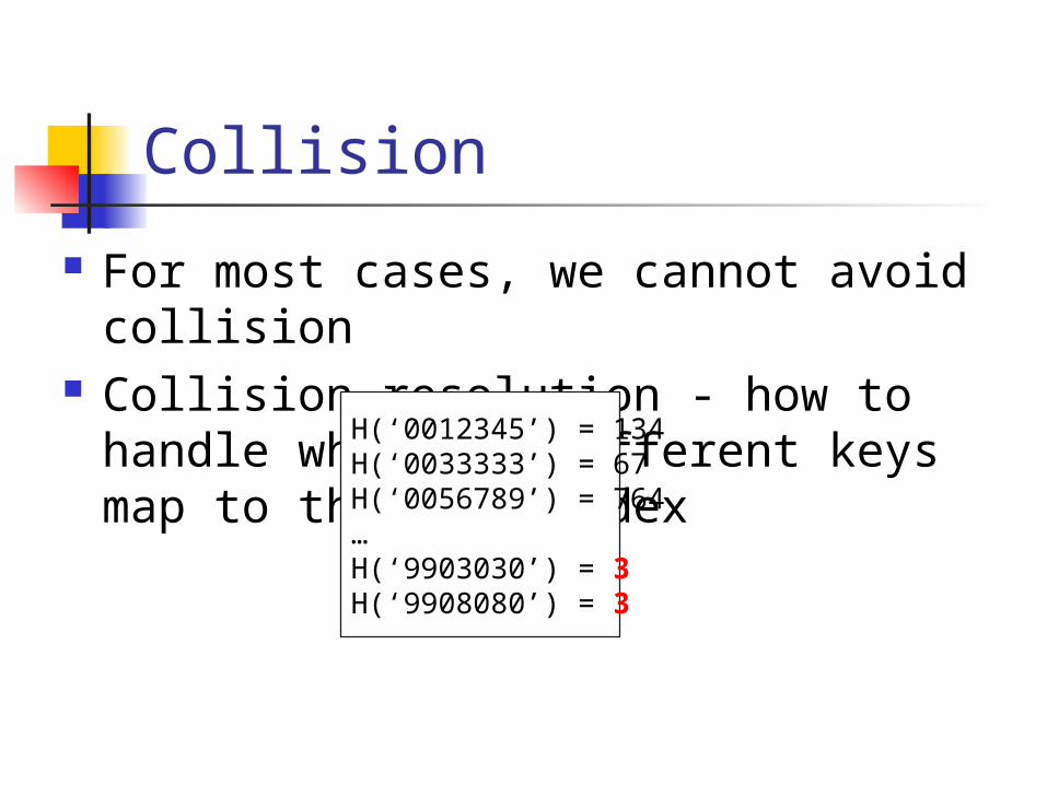
Collision

For most cases, we cannot avoid collision

Collision resolution - how to handle when two different keys map to the same index

H(‘0012345’) = 134H(‘0033333’) = 67H(‘0056789’) = 764…H(‘9903030’) = 3H(‘9908080’) = 3

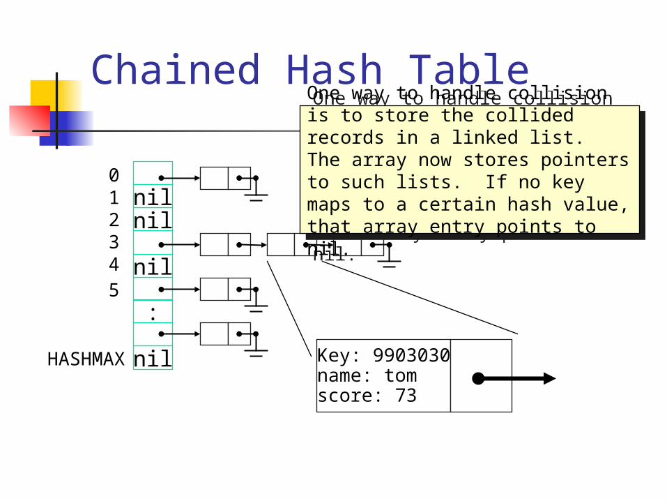
Chained Hash Table

2

4

10

3

nil

nilnil

5

nil

:

HASHMAX Key: 9903030name: tomscore: 73

One way to handle collision is to store the collided records in a linked list. The array now stores pointers to such lists. If no key maps to a certain hash value, that array entry points to nil.

One way to handle collision is to store the collided records in a linked list. The array now stores pointers to such lists. If no key maps to a certain hash value, that array entry points to nil.

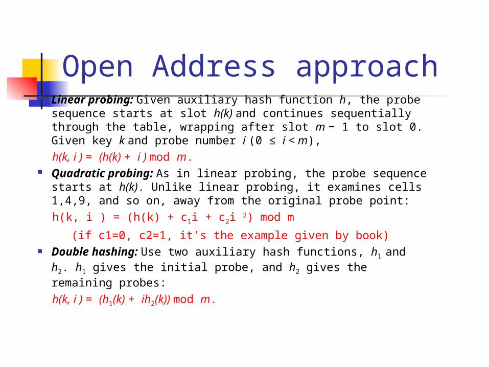
Open Address approach Linear probing: Given auxiliary hash function h, the probe

sequence starts at slot h(k) and continues sequentially through the table, wrapping after slot m − 1 to slot 0. Given key k and probe number i (0 ≤ i < m),

h(k, i ) = (h(k) + i ) mod m. Quadratic probing: As in linear probing, the probe sequence starts

at h(k). Unlike linear probing, it examines cells 1,4,9, and so on, away from the original probe point:

h(k, i ) = (h(k) + c1i + c2i 2) mod m

(if c1=0, c2=1, it’s the example given by book) Double hashing: Use two auxiliary hash functions, h1 and h2. h1

gives the initial probe, and h2 gives the remaining probes:

h(k, i ) = (h1(k) + ih2(k)) mod m.

Outline

Hash Table Recursion Sorting

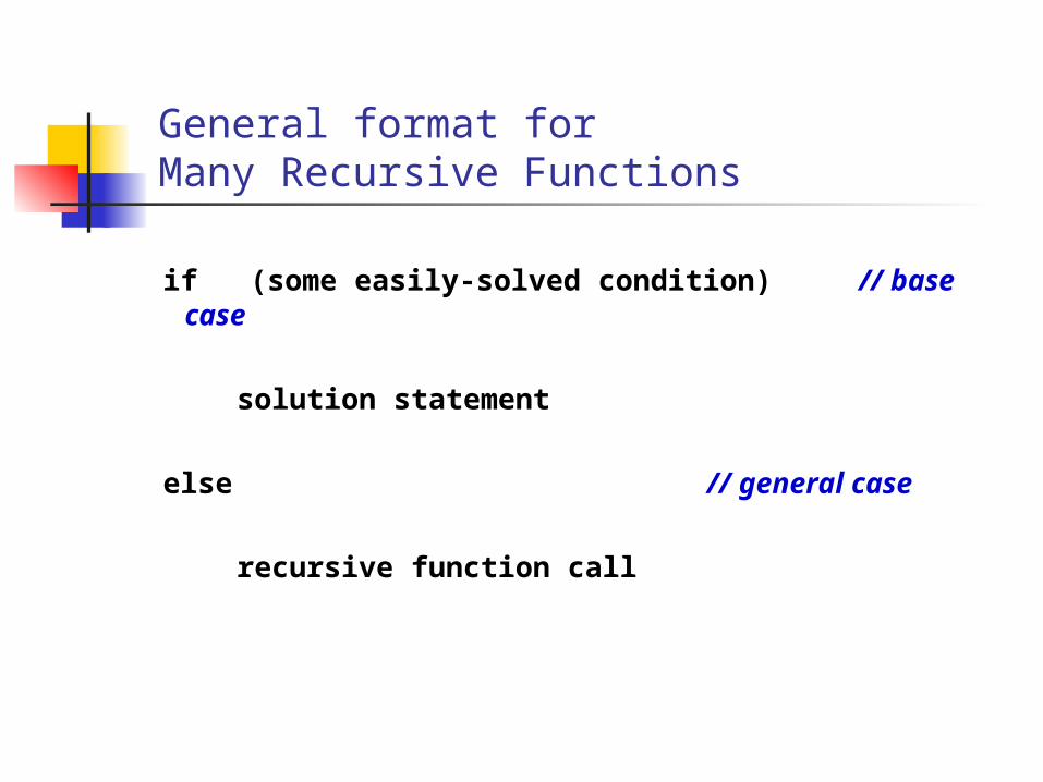
General format forMany Recursive Functions

if (some easily-solved condition) // base case

solution statement

else // general case

recursive function call

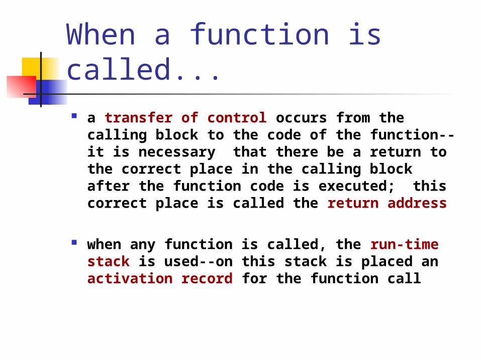
When a function is called... a transfer of control occurs from the

calling block to the code of the function--it is necessary that there be a return to the correct place in the calling block after the function code is executed; this correct place is called the return address

when any function is called, the run-time stack is used--on this stack is placed an activation record for the function call

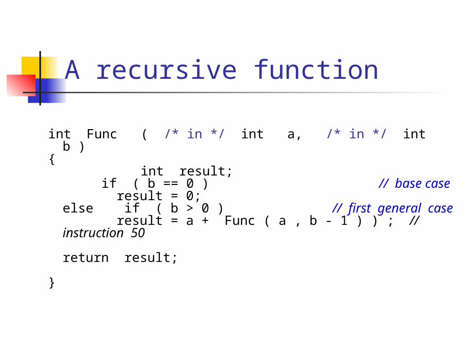
int Func ( /* in */ int a, /* in */ int b ){ int result; if ( b == 0 ) // base case

result = 0;else if ( b > 0 ) // first general

case result = a + Func ( a , b - 1 ) ) ; //

instruction 50

return result; }

A recursive function

FCTVAL ? result ? b 2 a 5Return Address 100

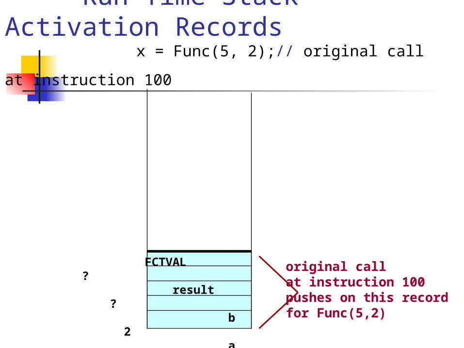
Run-Time Stack Activation Records

x = Func(5, 2);// original call at instruction 100

original call at instruction 100 pushes on this record for Func(5,2)

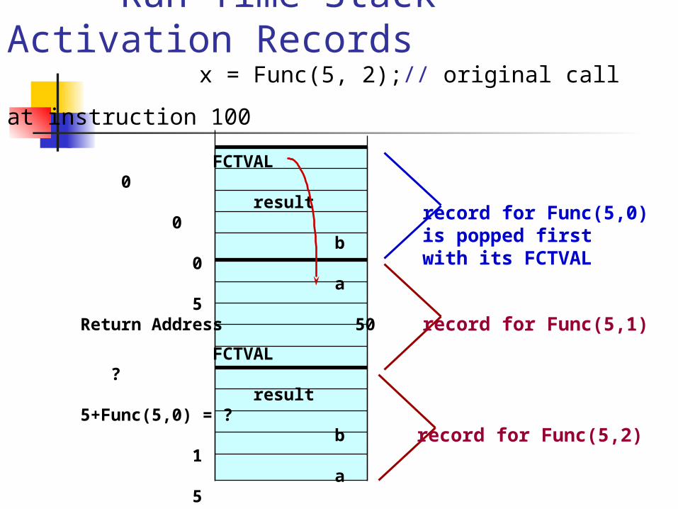
FCTVAL 0 result 0 b 0 a 5Return Address 50

FCTVAL ? result 5+Func(5,0) = ? b 1 a 5Return Address 50

FCTVAL ? result 5+Func(5,1) = ? b 2 a 5Return Address 100

record for Func(5,0)is popped first with its FCTVAL

record for Func(5,2)

record for Func(5,1)

Run-Time Stack Activation Records

x = Func(5, 2);// original call at instruction 100

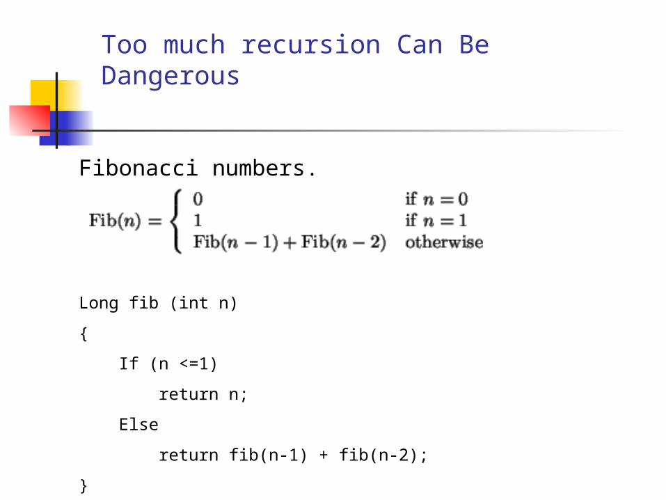
Too much recursion Can Be Dangerous

Fibonacci numbers.

Long fib (int n)

{

If (n <=1)

return n;

Else

return fib(n-1) + fib(n-2);

}

Too much recursion Can Be Dangerous

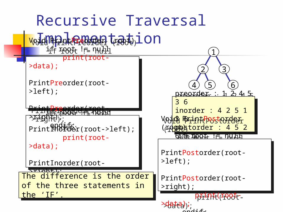
Recursive Traversal Implementation

Void PrintInorder (root) if root != null PrintInorder(root->left); print(root->data); PrintInorder(root->right); endif;

Void PrintInorder (root) if root != null PrintInorder(root->left); print(root->data); PrintInorder(root->right); endif;

The difference is the order of the three statements in the ‘IF’.

The difference is the order of the three statements in the ‘IF’.

1

2 3

4 5 6

preorder : 1 2 4 5 3 6inorder : 4 2 5 1 3 6postorder : 4 5 2 6 3 1

preorder : 1 2 4 5 3 6inorder : 4 2 5 1 3 6postorder : 4 5 2 6 3 1

Void PrintPreorder (root) if root != null print(root->data); PrintPreorder(root->left); PrintPreorder(root->right); endif;

Void PrintPreorder (root) if root != null print(root->data); PrintPreorder(root->left); PrintPreorder(root->right); endif;

Void PrintPostorder (root) if root != null PrintPostorder(root->left); PrintPostorder(root->right); print(root->data); endif;

Void PrintPostorder (root) if root != null PrintPostorder(root->left); PrintPostorder(root->right); print(root->data); endif;

Outline

Hash Table Recursion Sorting

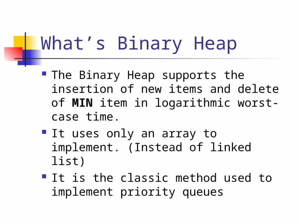
What’s Binary Heap

The Binary Heap supports the insertion of new items and delete of MIN item in logarithmic worst-case time.

It uses only an array to implement. (Instead of linked list)

It is the classic method used to implement priority queues

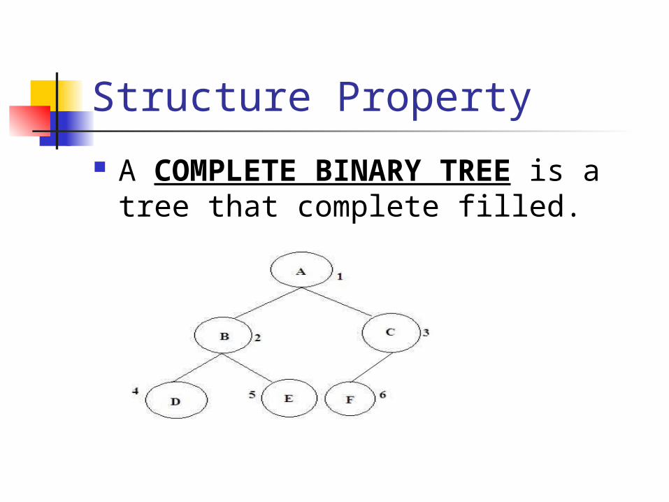
Structure Property

A COMPLETE BINARY TREE is a tree that complete filled.

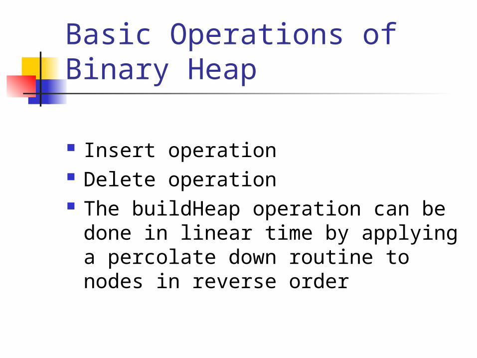
Basic Operations of Binary Heap

Insert operation Delete operation The buildHeap operation can be

done in linear time by applying a percolate down routine to nodes in reverse order

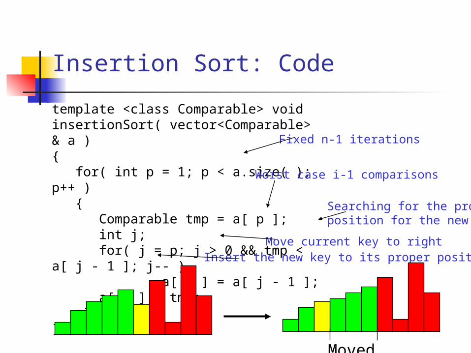
Insertion Sort: Code

template <class Comparable> void insertionSort( vector<Comparable> & a ) { for( int p = 1; p < a.size( ); p++ ) { Comparable tmp = a[ p ]; int j; for( j = p; j > 0 && tmp < a[ j - 1 ]; j-- ) a[ j ] = a[ j - 1 ]; a[ j ] = tmp; } }

Fixed n-1 iterations

Worst case i-1 comparisons

Move current key to rightInsert the new key to its proper position

Searching for the proper position for the new key

Moved

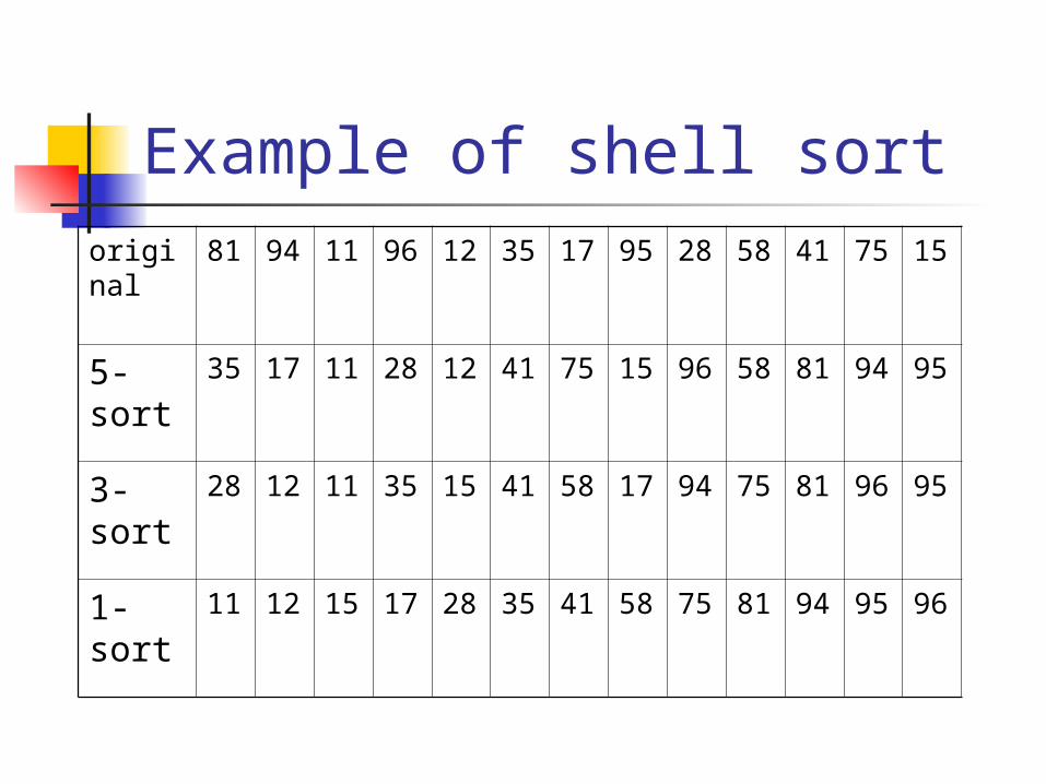
Example of shell sortoriginal

81 94 11 96 12 35 17 95 28 58 41 75 15

5-sort

35 17 11 28 12 41 75 15 96 58 81 94 95

3-sort

28 12 11 35 15 41 58 17 94 75 81 96 95

1-sort

11 12 15 17 28 35 41 58 75 81 94 95 96

27

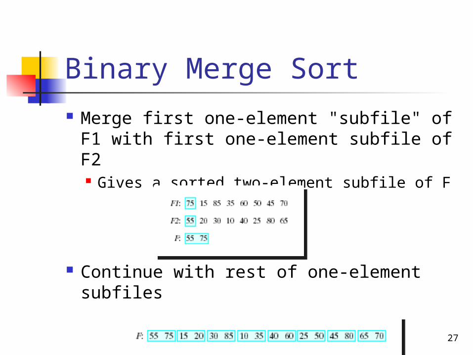
Binary Merge Sort

Merge first one-element "subfile" of F1 with first one-element subfile of F2 Gives a sorted two-element subfile of F

Continue with rest of one-element subfiles

Quicksort

Choose some element called a pivot

Perform a sequence of exchanges so that All elements that are less than this

pivot are to its left and All elements that are greater than the

pivot are to its right.

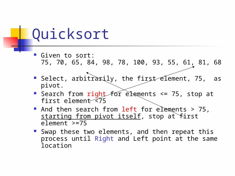
Quicksort Given to sort:

75, 70, 65, 84, 98, 78, 100, 93, 55, 61, 81, 68

Select, arbitrarily, the first element, 75, as pivot. Search from right for elements <= 75, stop at

first element <75 And then search from left for elements > 75,

starting from pivot itself, stop at first element >=75

Swap these two elements, and then repeat this process until Right and Left point at the same location

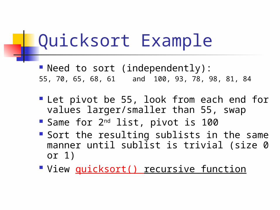
Quicksort Example Need to sort (independently):55, 70, 65, 68, 61 and 100, 93, 78, 98, 81, 84

Let pivot be 55, look from each end for values larger/smaller than 55, swap

Same for 2nd list, pivot is 100 Sort the resulting sublists in the same

manner until sublist is trivial (size 0 or 1)

View quicksort() recursive function

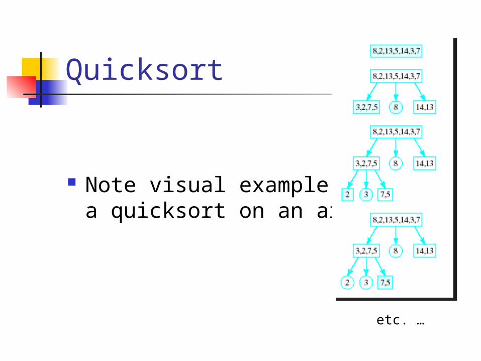
Quicksort

Note visual example ofa quicksort on an array

etc. …

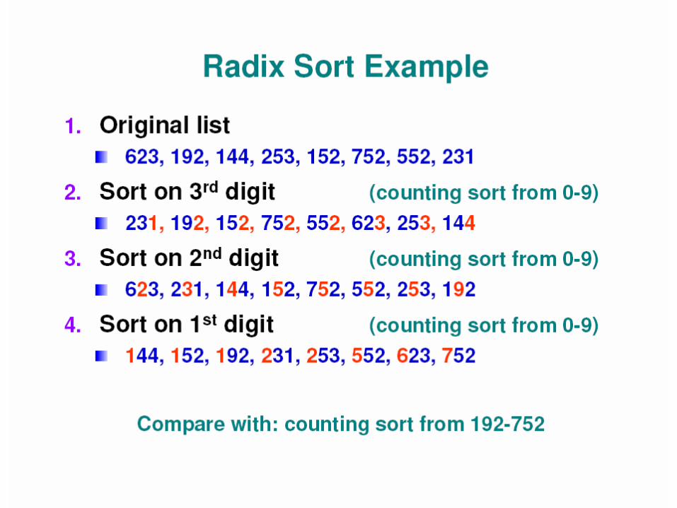
Radix Sort

Approach 1. Decompose key C into components

C1, C2, … Cd Component d is least significant, Each

component has values over range 0..k