Final Thesis Lissa Marten - mmss.wcas.northwestern.edummss.wcas.northwestern.edu/thesis/articles/get/880/Marten2015.pdf · increase!at!some!levels!of!Uber!surge,!this!findingindicatesthat

Assessing the Demand for Uber

Lissa Marten Thesis Advisor: Professor Ian Savage Instructor: Professor Joseph Ferrie

June 2015

1

EXEMPTION DETERMINATION April 16, 2015 Joseph Ferrie 2003 Sheridan Road Dept. of Economics Evanston, IL 847-491-8210 [email protected] Dear Dr. Joseph Ferrie:

The IRB reviewed the following submission:

Determination Date: 4/16/2015 Type of Submission: Initial Study

Review Level: Exempt Exempt Category (if

applicable): - (2) Tests, surveys, interviews, or observation

Title of Study: Assessing the Demand for Uber Principal Investigator: Joseph Ferrie

IRB ID: STU00200871 Funding Source: - Name: Economics

Grant ID: NU OSR Number:

IND, IDE, or HDE: None Documents Reviewed: • Recruitment email body, Category: Recruitment

Materials; • Social Behavioral Online Consent Template v2.doc, Category: Consent Form; • IRB Protocol, Category: IRB Protocol; • Survey Document, Category: Questionnaire/Survey

The IRB has determined that the study meets the criteria for exemption from IRB review and approval.

In conducting this study, you are required to follow the requirements listed in the Northwestern University (NU) Investigator Manual (HRP-103), which can be found by navigating to the IRB Library within the eIRB+ system.

2

This determination applies only to the activities described in the eIRB+ submission and does not apply should any changes be made. If changes are being considered and there are questions about whether IRB review is needed, please contact the IRB Office to discuss those changes. An exemption determination does not constitute nor guarantee institutional approval and/or support. Investigators and study team members must comply with all applicable federal, state, and local laws, as well as NU Policies and Procedures, which may include obtaining approval for your research activities from other individuals or entities.

For IRB-related questions, please consult the NU IRB website at http://irb.northwestern.edu. For general research questions, please consult the NU Office for Research website at http://www.research.northwestern.edu.

Sincerely,

Heather Gipson IRB Director

3

Table of Contents

IRB Exemption Certificate……………………………………………………………………………………………… 1

Acknowledgments…………………………………………………………………………………………………………. 4

Abstract………………………………………………………………………………………………………………………… 5

Introduction………………………………………………………………………………………………………….………. 6

Literature Review……………………………………………………………………………………………………..…… 8

Methodology……………………………………………………………………………………………………………….. 12

Survey……………………………………………………………………………………………………………………….... 18

Data……………………………………………………………………………………………………………………………. 23

Description of Variables………………………………………………………………………………………………. 25

Summary Statistics……………………………………………………………………………………………………… 27

Results and Statistical Analyses……………………………………………………………………………………. 28

Models……………………………………………………………………………………………………………… 29

Log-‐Likelihood Comparison………………………………………………………………………………. 41

Value of Time Discussion………………………………………………………………………………...… 42

Conclusion and Limitations………………………………………………………………………………………..… 46

Works Cited………………………………………………………………………………………………………………… 48

4

Acknowledgments

I would first like to thank Professor Ian Savage. Without his help, my thesis would

not have been possible. Professor Savage was there to encourage and assist me any time I

needed him, and for that, I am extremely grateful. My thesis would also not have been

possible without the assistance of Professor Amanda Stathopoulos; she aided me in every

bit of analysis and kindly taught me how to use the program Biogeme. She helped me out of

the kindness of her heart, and I am very thankful. I would also like to thank Professor

Joseph Ferrie for answering my many questions throughout the year, as well as having

incredible patience. I would like to thank Sarah Muir Ferrer, for her support throughout all

of my MMSS classes, but especially for her understanding presence. I wish to also thank

Professor William Rogerson for his leadership and guidance as director of the MMSS

program. Without him, none of this would be possible. Finally, I would like to thank my

friends. My friends have listened to me and advised me regarding my thesis and MMSS

classes throughout my four years at Northwestern, and I could not have done this without

them. I would like to give a special thank you to Ashley Augustine; I never would have

joined the MMSS program without her. Lastly, my biggest thank you goes to my family. My

parents have supported me every step of the way, through all my highs and lows, and I

would not be here without them. And to Carly-‐ you are the best sister I could ask for.

5

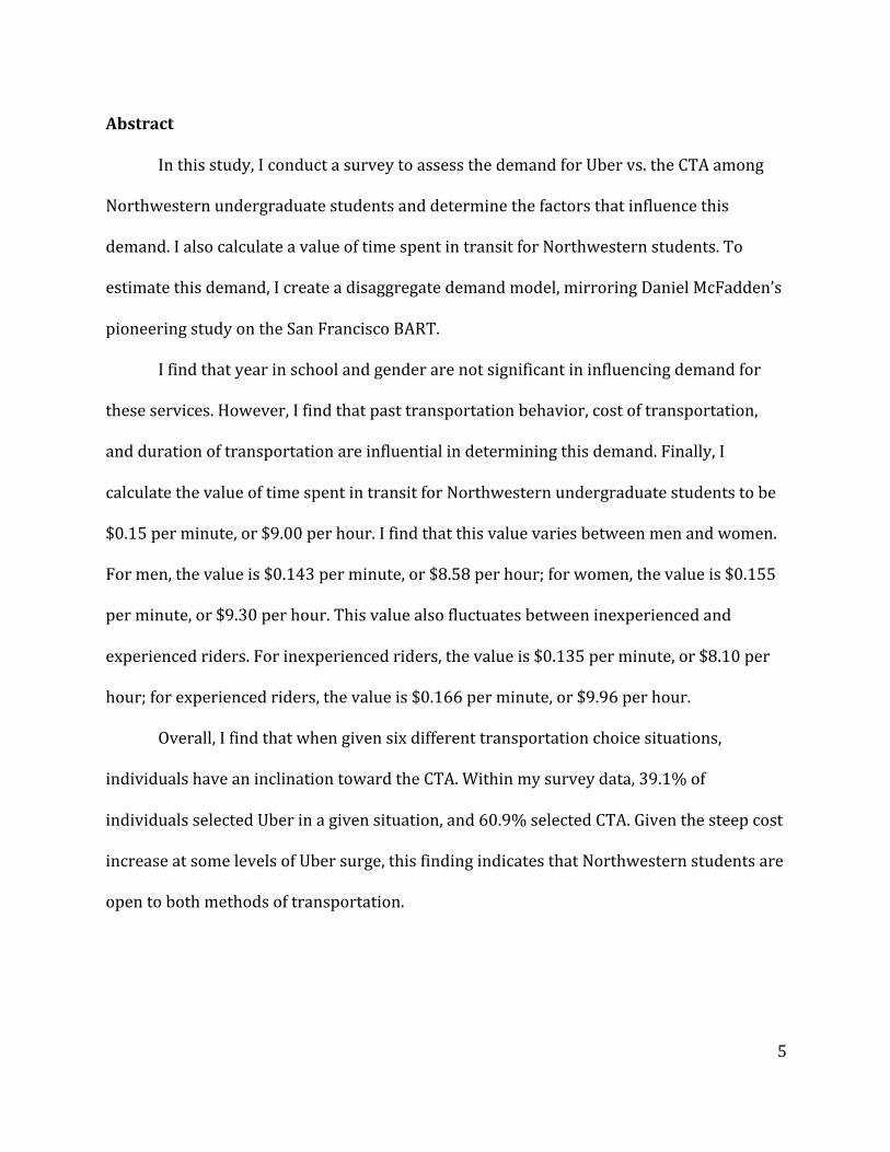
Abstract

In this study, I conduct a survey to assess the demand for Uber vs. the CTA among

Northwestern undergraduate students and determine the factors that influence this

demand. I also calculate a value of time spent in transit for Northwestern students. To

estimate this demand, I create a disaggregate demand model, mirroring Daniel McFadden’s

pioneering study on the San Francisco BART.

I find that year in school and gender are not significant in influencing demand for

these services. However, I find that past transportation behavior, cost of transportation,

and duration of transportation are influential in determining this demand. Finally, I

calculate the value of time spent in transit for Northwestern undergraduate students to be

$0.15 per minute, or $9.00 per hour. I find that this value varies between men and women.

For men, the value is $0.143 per minute, or $8.58 per hour; for women, the value is $0.155

per minute, or $9.30 per hour. This value also fluctuates between inexperienced and

experienced riders. For inexperienced riders, the value is $0.135 per minute, or $8.10 per

hour; for experienced riders, the value is $0.166 per minute, or $9.96 per hour.

Overall, I find that when given six different transportation choice situations,

individuals have an inclination toward the CTA. Within my survey data, 39.1% of

individuals selected Uber in a given situation, and 60.9% selected CTA. Given the steep cost

increase at some levels of Uber surge, this finding indicates that Northwestern students are

open to both methods of transportation.

6

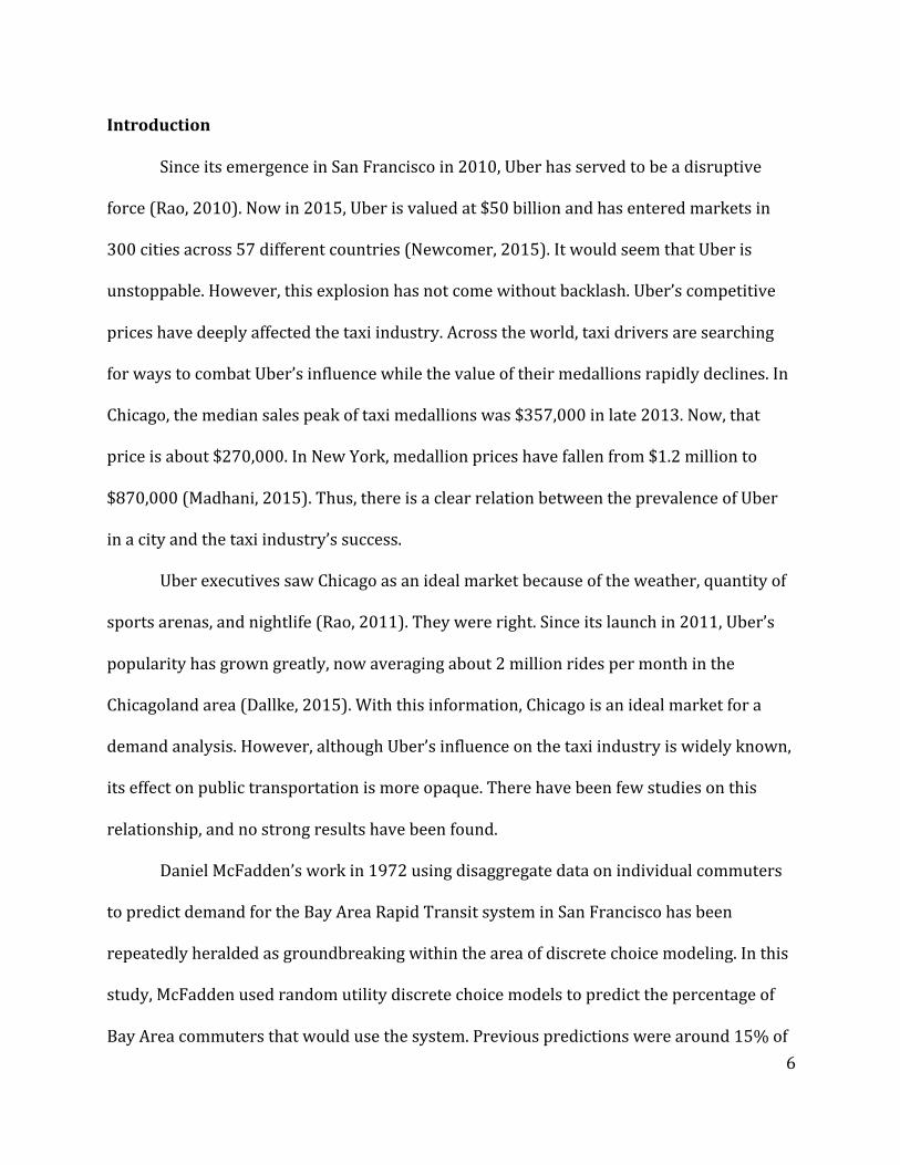
Introduction

Since its emergence in San Francisco in 2010, Uber has served to be a disruptive

force (Rao, 2010). Now in 2015, Uber is valued at $50 billion and has entered markets in

300 cities across 57 different countries (Newcomer, 2015). It would seem that Uber is

unstoppable. However, this explosion has not come without backlash. Uber’s competitive

prices have deeply affected the taxi industry. Across the world, taxi drivers are searching

for ways to combat Uber’s influence while the value of their medallions rapidly declines. In

Chicago, the median sales peak of taxi medallions was $357,000 in late 2013. Now, that

price is about $270,000. In New York, medallion prices have fallen from $1.2 million to

$870,000 (Madhani, 2015). Thus, there is a clear relation between the prevalence of Uber

in a city and the taxi industry’s success.

Uber executives saw Chicago as an ideal market because of the weather, quantity of

sports arenas, and nightlife (Rao, 2011). They were right. Since its launch in 2011, Uber’s

popularity has grown greatly, now averaging about 2 million rides per month in the

Chicagoland area (Dallke, 2015). With this information, Chicago is an ideal market for a

demand analysis. However, although Uber’s influence on the taxi industry is widely known,

its effect on public transportation is more opaque. There have been few studies on this

relationship, and no strong results have been found.

Daniel McFadden’s work in 1972 using disaggregate data on individual commuters

to predict demand for the Bay Area Rapid Transit system in San Francisco has been

repeatedly heralded as groundbreaking within the area of discrete choice modeling. In this

study, McFadden used random utility discrete choice models to predict the percentage of

Bay Area commuters that would use the system. Previous predictions were around 15% of

7

area users, but McFadden predicted usage to be 6.3%—extremely close to the true value of

6.2% (Smith, 2014). McFadden later won a Nobel Prize for his pioneering work in discrete

choice modeling. His work serves as the basis of my model.

Many economists have performed similar studies, comparing the tradeoff between

various modes of transportation. However, a study of the sort has not been completed

using transportation network providers, such as Uber, Lyft, and Sidecar, which have come

to fruition in recent years. For the purposes of this study, I will collectively refer to all

transportation network providers as “Uber,” since Uber has been the most influential

player in the market so far.

In this study, I perform an analysis to assess the demand for Uber vs. the CTA among

Northwestern students. Specifically, I wish to determine what factors strongly influence

this demand and what a student’s value of time spent in transit is. To measure this demand,

I create a disaggregate demand model using data I have collected through an electronic

survey and perform an analysis. I hope for my research to be influential to future users of

both public transportation and Uber.

8

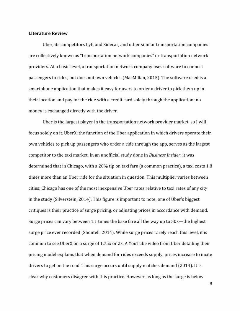
Literature Review

Uber, its competitors Lyft and Sidecar, and other similar transportation companies

are collectively known as “transportation network companies” or transportation network

providers. At a basic level, a transportation network company uses software to connect

passengers to rides, but does not own vehicles (MacMillan, 2015). The software used is a

smartphone application that makes it easy for users to order a driver to pick them up in

their location and pay for the ride with a credit card solely through the application; no

money is exchanged directly with the driver.

Uber is the largest player in the transportation network provider market, so I will

focus solely on it. UberX, the function of the Uber application in which drivers operate their

own vehicles to pick up passengers who order a ride through the app, serves as the largest

competitor to the taxi market. In an unofficial study done in Business Insider, it was

determined that in Chicago, with a 20% tip on taxi fare (a common practice), a taxi costs 1.8

times more than an Uber ride for the situation in question. This multiplier varies between

cities; Chicago has one of the most inexpensive Uber rates relative to taxi rates of any city

in the study (Silverstein, 2014). This figure is important to note; one of Uber’s biggest

critiques is their practice of surge pricing, or adjusting prices in accordance with demand.

Surge prices can vary between 1.1 times the base fare all the way up to 50x—the highest

surge price ever recorded (Shontell, 2014). While surge prices rarely reach this level, it is

common to see UberX on a surge of 1.75x or 2x. A YouTube video from Uber detailing their

pricing model explains that when demand for rides exceeds supply, prices increase to incite

drivers to get on the road. This surge occurs until supply matches demand (2014). It is

clear why customers disagree with this practice. However, as long as the surge is below

9

1.8x in Chicago, Uber is less expensive than a taxi, leading to great problems in the taxi

industry.

The Uberx experience differs from the taxi experience in many ways. While the

majority of taxi drivers work full time, 80% of Uber drivers work part time. The hourly pay

for drivers varies wildly, but one study quotes the average pay per hour in Chicago as being

$16.20 per hour for Uber drivers and $11.87 per hour for taxi drivers (Lawler, 2015). Uber

is often seen as safer than taxis as well. The app employs a rating system in which

passengers rate drivers after every ride, and vice versa. Drivers who consistently receive

low ratings are required to take a training course, and can later be suspended from the app

(Smith IV, 2015). This process ensures that riders know who their driver is and that the

driver is held accountable for any misdoings—a practice that is not followed as carefully in

the taxi industry.

Based on studies conducted and personal experience, the customer base for Uber

and taxis varies as well. A Skift.com study found that the most frequent users are older

millennials—individuals aged 25-‐34. They also determined that males use the apps more

than women, but women are more aware of the apps. Finally, they found that heaviest

users are wealthier millennials—individuals earning $150,000 or more in income—and

that individuals at the lowest end of the income bracket have much less knowledge of these

applications (Ali, 2015). Taxis are less limiting, as they don’t require the user to own a

smartphone.

Because of the differing user bases, the demand for the two modes differs as well.

There is no specific research directly assessing from what modes the Uber demand is

coming, but one may assume that much of it stems from former taxi riders, personal vehicle

10

drivers, and public transit users. The latter is the basis of this study. Furthermore, in

regards to public transportation, the demographics of individuals who would employ this

method of transit vary wildly as well. In a 2007 study by the American Public

Transportation Association, several important findings were reported. One outcome is that

users of public transportation have a varying range of incomes: 20.1% of riders have a

household income of less than $15,000, 45.6% from $15,000 to $49,999, 24.8% from

$50,000 to $99,999, and 9.5% have a household income of $100,000 or more (Neff & Pham,

2007, p. 7). All incomes reported are in 2004 dollars. As shown above, the incomes of

individuals who frequently utilize public transportation are quite different than the

heaviest users of Uber—those with incomes of $150,000 or more (Ali, 2015).

In Chicago, the most utilized form of public transportation is the Chicago Transit

Authority (CTA). The CTA is the second largest public transportation system in the country,

with 1.7 million rides taken per day. The CTA’s “L” train (short for elevated) operates over

224 miles of track, including to many Chicago suburbs (CTA Facts at a Glance). The CTA has

a train route that operates between Evanston and downtown Chicago, which many

Northwestern students frequent. Often, the CTA serves as a viable option for students to

use in transporting themselves around the city.

While there have been some articles looking into the effect Uber’s entrance into the

market has had on the value of taxi medallions, there have been no studies linking Uber and

public transportation. In order to assess these differences in demand, one must determine

the major factors influencing individual decisions in choosing a method of transportation.

The tradeoff between public transportation and Uber is a cost versus time saving decision.

It also begs the question: What is an individual’s value of time spent in transit? Because

11

sharing an Uber ride with other individuals can make the cost of an Uber ride only slightly

higher than that of public transportation, this is a reasonable tradeoff to assess. In regards

to pricing, the surge pricing function for Uber is essential. Although Uber’s base prices are

relatively inexpensive—especially compared to a taxi ride—their surge prices can cause

the fare to skyrocket, creating an added wrinkle in the Uber vs. public transit dilemma.

Individuals who choose to take Uber when there is a high surge have a very high value of

time spent in transit. However, other factors are likely to influence this tradeoff as well,

such as gender, amount of money typically spent on transportation costs, age, etc. This is

what I aim to determine.

12

Methodology

One successful method of assessing demand for mode choice is that of discrete

choice modeling. In fact, the methods for analyzing discrete choices were developed

specifically in the field of transportation economics (Savage, 2014, p. 34). McFadden (1978)

explains that disaggregate models begin with the idea that travel demand is generated by

observed individual choice behavior, or a maximization of utility (p. 2). Moreover,

disaggregate behavioral forecasting does not mandate one model; rather, it serves as a

system for building models. Data observed through disaggregate analysis takes the form of

a discrete choice, i.e. representing one variable by 0 and one by 1 (McFadden, 1978, p. 2).

Alternatively, aggregate models are based on observed choices for groups of

individuals, or on average choices at the zone level (Ortúzar & Willumsen, 2011, p. 227).

While aggregate models look at average decisions that have previously been made,

disaggregate models examine individual choices in hypothetical situations. In fact,

disaggregate models may be more efficient than aggregate models in regards to data

required. In aggregate modeling, an observation can be the average of many individual

observations. In disaggregate modeling, each individual choice represents an observation

in the model, leading to the potential for less necessary data than in aggregate models.

Disaggregate models are also less likely to incur biases that can occur in aggregate models

as a result of hidden or unidentified characteristics (Ortúzar & Willumsen, 2011, p. 228-‐

229). Finally, disaggregate models are often used to discuss transportation mode choice, so

they serve as an excellent basis for this analysis (Savage, 2014, p. 34).

Another distinction between aggregate and disaggregate models is the use of

revealed preference data vs. stated preference data. When data is used to describe a

13

traveler’s preference within actual decision making, it is called revealed preference data.

When respondents are asked about hypothetical situations, their responses create stated

preference data. Stated preference methods are especially useful for new developments in

transit or hypothetical price changes; McFadden used this method in his study on the San

Francisco BART, as the BART had yet been opened at the time of his study. Stated

preference data allows the values in question to vary much more widely than revealed

preference data, as it is difficult to determine the effect of a change in transit when user’s

previous behavior is the only known data. However, many researchers are hesitant to trust

in individual responses regarding hypothetical situations. Combining the two methods is

truly ideal. In fact, McFadden did just this in his study. After the BART began to operate, he

combined the stated preference data gathered with revealed preference data on actual user

patterns. Overall, my study incorporates solely stated preference data, but I have controlled

for many researchers’ concern of respondents answering questions about which they lack

knowledge by eliminating all participants who have never taken these methods of

transportation previously (Small & Winston, 1999, p. 33-‐34).

According to Juan de Dios Ortúzar and Luis G. Willumsen, discrete choice models are

based on the probability of individuals selecting a certain option. Moreover, their choices

are a function of their socioeconomic characteristics and the relative appeal of a certain

option (2011, p. 227). Thus, one’s utility varies based on individual factors such as travel

time and cost. Moreover, another important factor to note is that disaggregate models are

probabilistic; they indicate the probability of choosing each alternative, but do not show

which alternative is ultimately selected (Ortúzar & Willumsen, 2011, p. 229). For my study,

I specifically focus on these characteristics and their influence on mode choice. Because of

14

the diverse groups of individuals utilizing the competing modes, determining the factors in

play with mode choice is essential.

Furthermore, Daniel McFadden explains that certain variables must be controlled

for. He provides the example of family size; this can vary one’s distance from public transit,

cost of transportation, and walk time. Disaggregate calibration methods do allow these

variables to be included, but it is also possible to use only conventional variables, which is

seen in my study. He explains that including variables other than traditional hindrances

may only slightly improve the model’s ability to explain observed choices within the data

(McFadden, 1978, p. 7). With this knowledge, I have limited my study to the Northwestern

undergraduate population, excluding all graduate students, so as to keep my population

somewhat homogeneous and control for individuals’ proximity to public transportation.

One benefit of disaggregate demand models is that they investigate people’s

individual choices. They use the true values of variables that each individual is faced with,

rather than average values, which can often hide varying information (Small & Winston,

1999, p. 15). These models assume that an individual’s utility is made up of two parts. The

first part is systematic; it can be predicted based on existing features of the respondent and

of the transit mode itself. In my model, I look at user characteristics such as gender, year in

school, and number of rides taken in the past, as well as choice characteristics including

length of time of each mode and cost of each mode. The second part is a random utility

component that cannot be predicted; it represents an individual’s distinctive inclination

toward a mode. Thus, two individuals with identical personal characteristics could have

distinctive preferences toward different modes of transit. In the case of Uber vs. the CTA,

there are many factors to individual decision making that are not accounted for in the

15

model, thus, it is important to keep the random utility component in mind. With this, we do

not know anything about the distribution of the values of the random utility element, so we

cannot predict precisely whether an individual will choose Uber or the CTA (Savage, 2014,

p. 34-‐35).

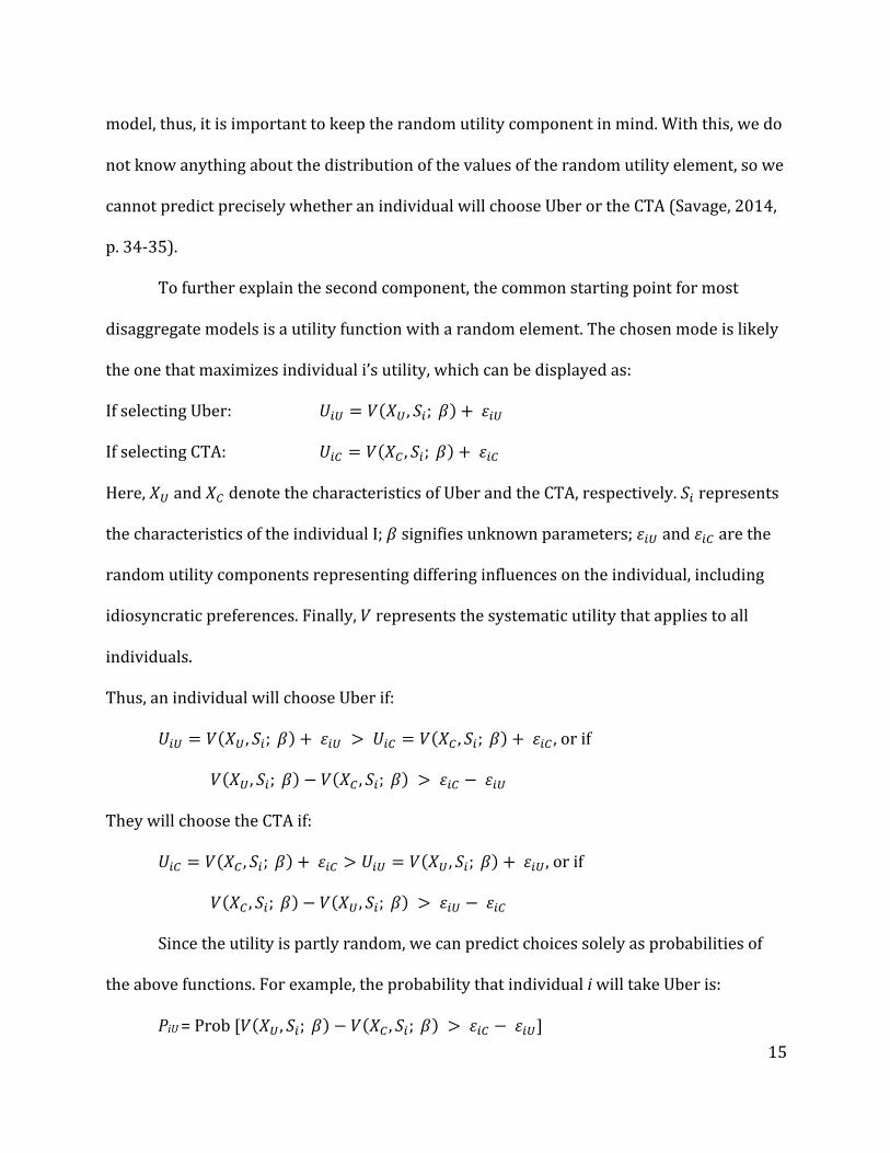
To further explain the second component, the common starting point for most

disaggregate models is a utility function with a random element. The chosen mode is likely

the one that maximizes individual i’s utility, which can be displayed as:

If selecting Uber: 𝑈!" = 𝑉 𝑋! , 𝑆!; 𝛽 + 𝜀!"

If selecting CTA: 𝑈!" = 𝑉 𝑋! , 𝑆!; 𝛽 + 𝜀!"

Here, 𝑋! and 𝑋! denote the characteristics of Uber and the CTA, respectively. 𝑆! represents

the characteristics of the individual I; 𝛽 signifies unknown parameters; 𝜀!" and 𝜀!" are the

random utility components representing differing influences on the individual, including

idiosyncratic preferences. Finally, 𝑉 represents the systematic utility that applies to all

individuals.

Thus, an individual will choose Uber if:

𝑈!" = 𝑉 𝑋! , 𝑆!; 𝛽 + 𝜀!" > 𝑈!" = 𝑉 𝑋! , 𝑆!; 𝛽 + 𝜀!" , or if

𝑉 𝑋! , 𝑆!; 𝛽 − 𝑉 𝑋! , 𝑆!; 𝛽 > 𝜀!" − 𝜀!"

They will choose the CTA if:

𝑈!" = 𝑉 𝑋! , 𝑆!; 𝛽 + 𝜀!" > 𝑈!" = 𝑉 𝑋! , 𝑆!; 𝛽 + 𝜀!" , or if

𝑉 𝑋! , 𝑆!; 𝛽 − 𝑉 𝑋! , 𝑆!; 𝛽 > 𝜀!" − 𝜀!"

Since the utility is partly random, we can predict choices solely as probabilities of

the above functions. For example, the probability that individual i will take Uber is:

PiU = Prob [𝑉 𝑋! , 𝑆!; 𝛽 − 𝑉 𝑋! , 𝑆!; 𝛽 > 𝜀!" − 𝜀!"]

16

The probability that individual i will take the CTA is:

PiC = Prob [𝑉 𝑋! , 𝑆!; 𝛽 − 𝑉 𝑋! , 𝑆!; 𝛽 > 𝜀!" − 𝜀!"]

Material from previous paragraphs derived from (Savage, 2014, p. 34-‐35) and from (Small

& Winston, 1999, p. 15-‐16)

A variety of frameworks can be used to show this model, however, I will be using the

multinomial logit model (MNL), which is the simplest and most popular model for discrete

choice (Ortúzar and Willumsen, 2011, p. 232). This model has choice probabilities in the

following form: [Share of the i-‐th alternative] = exp[mean utility of i-‐th alternative] /

{exp[mean utility of the first alternative] + … + exp[mean utility of the last alternative]}.

Because the structure of the mean utility function in MNL is based on individual behavior,

the form will be similar regardless of the aspect of transportation being studied, such as

distribution or mode split. Moreover, for homogeneous market segments—here, the

Northwestern undergraduate population—the utilization of the model is carried out at the

disaggregate level, rather than the aggregate level (McFadden, 1978, p. 5-‐7). Furthermore,

for my purposes, the demand curve will be vertical, as participants are only offered the

choice between Uber and the CTA. Abstaining from traveling is not an option, so it is

assumed that the trip is taking place.

McFadden’s study on the BART is still similar to my study in terms of the use of

discrete mode choice theory. In San Francisco, the BART served as a new mode of

transportation, similar to Uber, that put itself in a part of the travel spectrum that was

previously empty. Just as Uber has gained passengers who previously utilized taxis, drove

their own cars, or used public transportation, the BART took passengers from various

transit methods. In his study, McFadden surveyed 771 commuters in the Bay Area before

17

the BART was open, asking about their current transit mode, cost, and time, as well as

characteristics about each commuter. He then constructed a binary logit model to forecast

individual mode choice between the alternatives that would exist once the BART was

finished. After the BART was opened, he contacted each study participant to observe their

mode choice and compared those results

with the original findings. Overall, the

discrete choice models predicted the

individuals’ mode choices fairly accurately.

The predictions are shown here (Train,

2009, p. 71-‐74). Overall, this study mirrors the analysis shown here; it is unique, however,

as no discrete choice models have been previously constructed involving Uber as a transit

mode.

18

Survey

In thinking about this thesis and my data set, I knew that in order to assess the true

stated preferences of individuals, I would need to gather the data via a survey. Thus, I chose

to focus on Northwestern undergraduates as an easily accessible population who I knew

would be largely familiar with both methods of transportation.

After following the Northwestern Institutional Review Board approval process to

format the questions and language of my survey, I received a certificate of exemption

(certificate attached on page 1 of thesis). I was then able to distribute my survey. In April,

my survey was dispersed among various Northwestern listservs and Facebook groups. In

total, I received 572 responses. Participants were asked for background information,

including gender, year in school, average monthly spending on transportation (excluding

car ownership and operations costs), and the number of trips taken using Uber and/or the

CTA since the beginning of the school year (September 2014). Average monthly spending

on transportation was capped at $200 per month, and the number of trips taken using Uber

and/or the CTA was capped at 50 per transit method since September 2014.

Participants were also asked whether they had taken Uber or the CTA previously. If

they responded “no” to either of these two questions, the survey automatically concluded,

preventing those participants from reaching the travel situation questions (pictured

below). This decision was made based on the difficulty of assessing an individual’s

likelihood of choosing an unfamiliar method of transit. Thus, to eliminate bias, these

responses were removed from the survey; individuals who did not identify as

undergraduates were also eliminated. Finally, I removed responses from individuals who

had not completed the user characteristic or experience questions, providing me with little

19

information about their choices. After this removal process, I was left with 488 unique

responses in my sample.

The crux of the survey included three unique travel situation questions, each with

two different scenarios (pictured below). Each of the three questions asked the survey

participant to choose between a journey using Uber or the CTA. The trips included journeys

from Evanston to the Loop, Lincoln Park to the South Loop, and the West Loop to the East

Loop. The times and costs presented took on real world values to make the model as

accurate as possible. These specific scenarios were selected for their variability in time and

cost. Moreover, not traveling was not an option in my survey. Each initial question

presented a choice scenario between Uber and the CTA using one of the three journeys

above. In the initial question, the price of Uber did not have a surge. Each follow-‐up

question varied the price of the Uber journey, with the possible surges of 1.5, 1.75, and 2

times the original price. The price of the CTA journey did not vary between scenarios or

situations since the price of the CTA does not vary in the real world; it remained $2.25 for

each situation I presented. The length of each journey also remained the same for each

initial and follow up question.

All participants received the same initial travel situation, but received only one of

the three follow-‐up surge questions (1.5, 1.75, or 2 times the original price). Thus, about

one third of my respondents received each unique surge scenario. This allowed me to vary

the responses from my sample. Through these travel situation questions, I assigned a

binary value to the individual’s choice, allowing me to create a disaggregate demand model

for the choice of Uber vs. the CTA. For the purposes of my study, I assigned each response

20

the binary values of 1 (Uber) or 2 (CTA), with the value of 0 assigned to unanswered

options that I then excluded from the model.

Shown here are the three unique situations and one of three possible follow up

questions for each situation:

Situation 1: Evanston to the Loop

21

Situation 2: Lincoln Park to the South Loop

22

Situation 3: The West Loop to the East Loop

23

Data

In order to prepare the data, I first downloaded it from the Qualtrics survey

software and imported it into Excel. Once imported, I assigned each survey participant a

unique identifier and cleaned the data of questions that did not pertain to my model, such

as the respondents’ email addresses. In the initial import, the data was sorted so that each

row header contained the exact question participants had been asked. I coded each column

with a variable name that would later be used in the model. I filled all gaps in the data with

zeroes, so as not to cause an error in the model.

Finally, I cut the data and imported the time and cost information for each situation.

Initially, the data did not include the time and cost information that participants had been

asked. Each column was sorted with the situational question participants had seen and

populated with a 1 (Uber), 2 (CTA), or 0 (indicating they had not received that question),

showing their selection. I then cut the data so that each unique individual had twelve rows

attributed to him or her. This is equivalent to the number of possible discrete choice

situational questions that the survey contained—three unique questions, each with one

base case and three separate surge follow up questions, or twelve total questions. Each

participant received and responded to six total questions. The user characteristic and user

experience questions that did not vary were pasted identically into each of the twelve rows.

I then created Cost_Uber, Time_Uber, Cost_CTA, and Time_CTA variables indicating

the cost and time of each respective mode for a given situation. From this, a CHOICE

variable for each participant was formed. This is the most important variable in the model;

it indicates which choice participants had made with the given cost and time options

presented to them and allows the model to read in each row of data as corresponding to

24

one of the two unique choices. The CHOICE variable takes on the values of 1, 2, or 0, based

on the individual’s selection. Additionally, the model is coded to ignore each line of data

where CHOICE = 0. Using the base set of data, I was able to create new variables. With the

data formatted properly, I was continually able to sort it to spot check any results I was

finding when modeling to determine whether or not they appeared to be accurate. I also

created data tables to cut the data into smaller, sorted groups and analyze the appropriate

size of groups within subsets of my sample.

25

Description of Variables

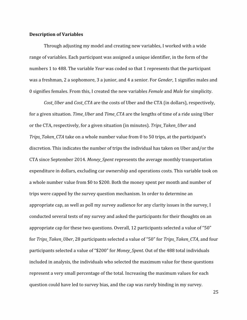
Through adjusting my model and creating new variables, I worked with a wide

range of variables. Each participant was assigned a unique identifier, in the form of the

numbers 1 to 488. The variable Year was coded so that 1 represents that the participant

was a freshman, 2 a sophomore, 3 a junior, and 4 a senior. For Gender, 1 signifies males and

0 signifies females. From this, I created the new variables Female and Male for simplicity.

Cost_Uber and Cost_CTA are the costs of Uber and the CTA (in dollars), respectively,

for a given situation. Time_Uber and Time_CTA are the lengths of time of a ride using Uber

or the CTA, respectively, for a given situation (in minutes). Trips_Taken_Uber and

Trips_Taken_CTA take on a whole number value from 0 to 50 trips, at the participant’s

discretion. This indicates the number of trips the individual has taken on Uber and/or the

CTA since September 2014. Money_Spent represents the average monthly transportation

expenditure in dollars, excluding car ownership and operations costs. This variable took on

a whole number value from $0 to $200. Both the money spent per month and number of

trips were capped by the survey question mechanism. In order to determine an

appropriate cap, as well as poll my survey audience for any clarity issues in the survey, I

conducted several tests of my survey and asked the participants for their thoughts on an

appropriate cap for these two questions. Overall, 12 participants selected a value of “50”

for Trips_Taken_Uber, 28 participants selected a value of “50” for Trips_Taken_CTA, and four

participants selected a value of “$200” for Money_Spent. Out of the 488 total individuals

included in analysis, the individuals who selected the maximum value for these questions

represent a very small percentage of the total. Increasing the maximum values for each

question could have led to survey bias, and the cap was rarely binding in my survey.

26

From this data, I created the variable CHOICE, which takes on a value of 1 if the

individual selected Uber for a given situation, 2 if they selected the CTA, and 0 if they did

not receive or answer the question. When modeling the data, I excluded the lines of data

where CHOICE was equal to 0. Trip_Ratio_Uber is equal to the ratio of Uber trips to the sum

of Uber and CTA trips, or total trips. Trip_Ratio_CTA is equal to the ratio of CTA trips to total

trips. Cost_Diff represents the difference in cost between Uber and CTA trips, for each

individual situation, expressed in dollars. In my models, I subtracted CTA cost from Uber

cost, so all values within the Cost_Diff variable are positive. Time_Diff represents the

difference in length between Uber and CTA trips, for each individual situation, expressed in

minutes. In my models, I subtracted CTA time from Uber time, so all values within the

Time_Diff variable are negative.

27

Summary Statistics

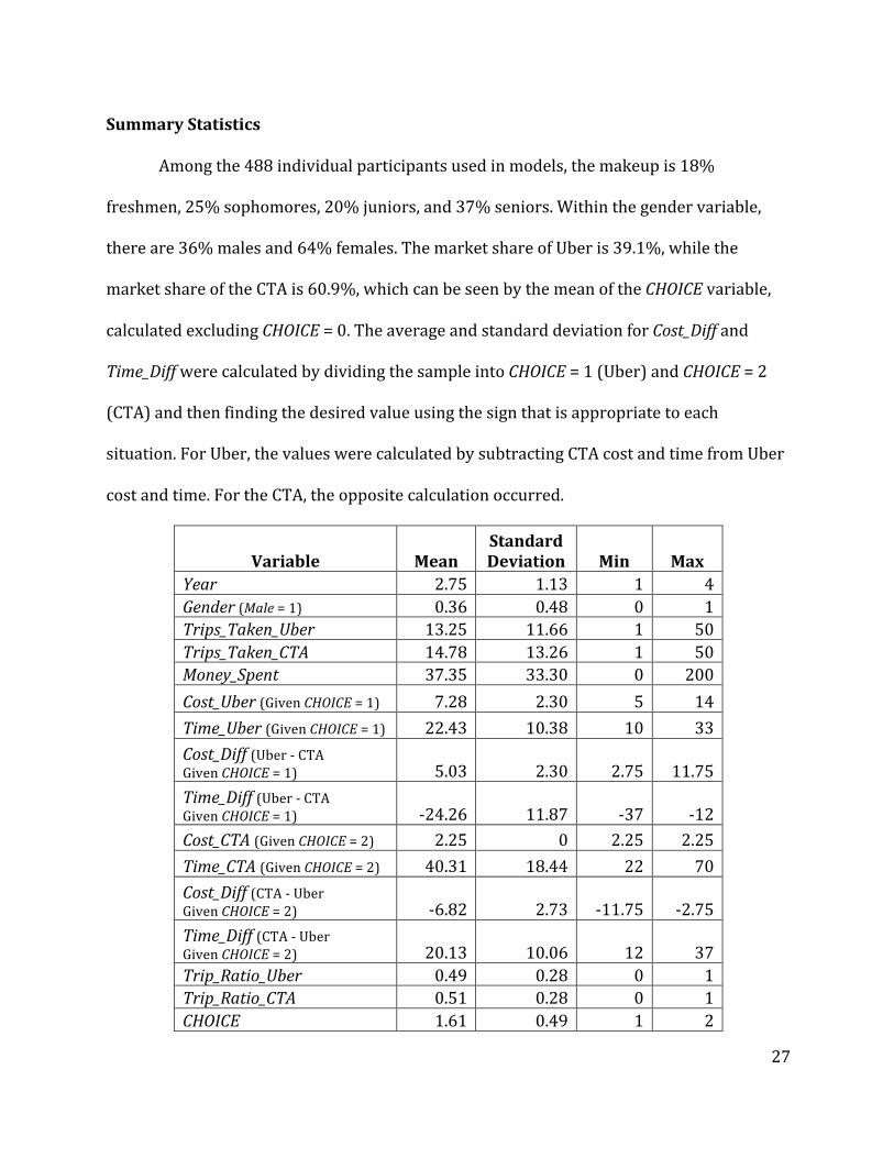
Among the 488 individual participants used in models, the makeup is 18%

freshmen, 25% sophomores, 20% juniors, and 37% seniors. Within the gender variable,

there are 36% males and 64% females. The market share of Uber is 39.1%, while the

market share of the CTA is 60.9%, which can be seen by the mean of the CHOICE variable,

calculated excluding CHOICE = 0. The average and standard deviation for Cost_Diff and

Time_Diff were calculated by dividing the sample into CHOICE = 1 (Uber) and CHOICE = 2

(CTA) and then finding the desired value using the sign that is appropriate to each

situation. For Uber, the values were calculated by subtracting CTA cost and time from Uber

cost and time. For the CTA, the opposite calculation occurred.

Variable Mean Standard Deviation Min Max

Year 2.75 1.13 1 4 Gender (Male = 1) 0.36 0.48 0 1 Trips_Taken_Uber 13.25 11.66 1 50 Trips_Taken_CTA 14.78 13.26 1 50 Money_Spent 37.35 33.30 0 200 Cost_Uber (Given CHOICE = 1) 7.28 2.30 5 14 Time_Uber (Given CHOICE = 1) 22.43 10.38 10 33 Cost_Diff (Uber -‐ CTA Given CHOICE = 1) 5.03 2.30 2.75 11.75 Time_Diff (Uber -‐ CTA Given CHOICE = 1) -‐24.26 11.87 -‐37 -‐12 Cost_CTA (Given CHOICE = 2) 2.25 0 2.25 2.25 Time_CTA (Given CHOICE = 2) 40.31 18.44 22 70 Cost_Diff (CTA -‐ Uber Given CHOICE = 2) -‐6.82 2.73 -‐11.75 -‐2.75 Time_Diff (CTA -‐ Uber Given CHOICE = 2) 20.13 10.06 12 37 Trip_Ratio_Uber 0.49 0.28 0 1 Trip_Ratio_CTA 0.51 0.28 0 1 CHOICE 1.61 0.49 1 2

28

Results and Statistical Analyses My analysis was completed in a software called Biogeme, an open source freeware

designed for the estimation of discrete choice models. This software is readily available

online. I used this software at the recommendation of Professor Amanda Stathopoulos, as it

is often used to model transportation choices. The model is a multinomial logit model, and

it is used to predict the individual utilities of the choice between Uber and CTA transit

modes. The left hand side of the model represents the utility of each individual choice,

while the right hand side shows the explanatory variables that go into the model, as well as

the intercept for each mode. This includes both personal characteristics about individual

travelers, as well as experience and user characteristic variables.

For each model displayed here, the left side of the Uber and CTA functions

represents the utilities of each alternative. The right side of each function includes

explanatory variables. Here, Cost_Diff, Time_Diff, Female, Freshman, Sophomore, Junior,

Money_Spent, Trip_Ratio_Uber, Trips_Taken_Uber, Time_Uber, and Surge were regressed on

the CHOICE = 1 variable, indicating the participant selected “Uber” in the situational choice

questions. The variables Trips_Taken_CTA and Time_CTA were regressed on the CHOICE = 2

variable, indicating the participant selected “CTA” in the situational choice questions. It is

important to keep in mind which alternative the variables are being regressed on, as the

coefficient for each variable changes sign accordingly. The models shown here contain

differing combinations of these variables, and each function is displayed above the output.

29

Model 1-‐ Base model

𝑈𝑏𝑒𝑟 = 𝐴𝑆𝐶!"#$ ∗ 𝑜𝑛𝑒 + 𝛽!"#$%"&& ∗ 𝑇𝑖𝑚𝑒_𝐷𝑖𝑓𝑓 + 𝛽!"#$%&'' ∗ 𝐶𝑜𝑠𝑡_𝐷𝑖𝑓𝑓

+ 𝛽!"#$!!"# ∗ 𝐹𝑟𝑒𝑠ℎ𝑚𝑎𝑛 + 𝛽!"#!!"!#$ ∗ 𝑆𝑜𝑝ℎ𝑜𝑚𝑜𝑟𝑒 + 𝛽!"#$%& ∗ 𝐽𝑢𝑛𝑖𝑜𝑟

+ 𝛽!"#$"% ∗ 𝐹𝑒𝑚𝑎𝑙𝑒 + 𝛽!"#$%&'$#( ∗𝑀𝑜𝑛𝑒𝑦_𝑆𝑝𝑒𝑛𝑡

+ 𝛽!"#$_!"#$%_!"#$ ∗ 𝑇𝑟𝑖𝑝_𝑅𝑎𝑡𝑖𝑜_𝑈𝑏𝑒𝑟

𝐶𝑇𝐴 = 𝐴𝑆𝐶!"# ∗ 𝑜𝑛𝑒

After creating a variety of models, this model served to be the best choice for the

data, including choice variables, user characteristics, and experience variables. Displayed

first in the output are the coefficients ASC_UBER and ASC_CTA. They serve as intercepts in

the model; one is always held constant. The abbreviation ASC represents the term

“Alternative Specific Constant.” In the model, they appear as “ASC_UBER * one” and

“ASC_CTA * one” to indicate that they are not multiplied by a variable. With ASC_CTA held

constant, the intercept for Uber takes on a negative value. This intercept represents all

unobserved effects that are unaccounted for in the model. Here, the unobserved effects are

inclined toward Uber. When Uber is held constant, the CTA intercept simply takes on the

opposite of the Uber intercept.

30

The two essential choice variables corresponding to the decisions participants made

are Cost_Diff and Time_Diff, shown here with the coefficients of BETA_COSTDIFF and

BETA_TIMEDIFF, respectively. As I explained previously, to calculate these differences, CTA

cost was subtracted from Uber cost, and CTA time from Uber time, respectively. The

rationale for calculating the difference is that in this model, since participants were asked

to choose one of two modes of transportation when not traveling was not an option, it was

necessary to look at the gap between these two values, rather than the true values for each

mode. For those travelers who have an extremely high value of time, they may be inclined

to choose Uber, regardless of the surge cost. For those who have an extremely low value of

time, they may select CTA regardless of the shorter time duration of an Uber ride. However,

for those travelers who have a value of time in between these extremes, looking at their

choices as the time and cost gaps widen becomes essential to determining the overall value

of time spent traveling.

In regards to BETA_COSTDIFF, when regressed on the utility of Uber, the coefficient

takes on a significant value of -‐0.370. This affirms my hypothesis; as the cost of an Uber

ride rises (often due to surge), the individual traveler is less likely to choose that method of

transportation, and instead switch to the CTA. BETA_TIMEDIFF is very significant as well,

and it takes on a value of -‐0.0556. This variable is a bit more complex. While Cost_Diff takes

on positive values, Time_Diff takes on negative values. As the length of an Uber ride

increases, the gap between the two values shrinks, assuming CTA ride length has not

changed. For example, if the initial values for time are 30 minutes for Uber and 70 minutes

for CTA, the difference between the two is 40 minutes, or for our purposes, -‐40. If the Uber

time increases to 40 minutes, the difference between the two is now 30 minutes, or -‐30.

31

Thus, as the length of time in an Uber ride increases, the difference between the two

shrinks, and Cost_Diff moves toward 0. At the same time, the likelihood of choosing Uber

decreases, as corroborated by the coefficient of -‐0.0556. Thus, both variables indicate an

inclination toward the CTA, which holds true in the data.

Although the cost and time variables are essential to this model, the user

characteristics serve to be important as well. While the Female variable does have a

positive inclination toward Uber, it does not prove to be significant in this model, indicating

that gender is not significant in determining whether an individual will select Uber or the

CTA. This is an important finding. My initial hypothesis was that females would be highly

likely to choose Uber over the CTA; the CTA is often seen as unsafe, and Uber ensures a safe

journey from door to door. However, although there is an inclination toward Uber for

women, it is not significant in this model. A similar trend occurred with Year. Initially, I

hypothesized that as year in school increased, individuals would be more likely to take

Uber. From personal experience, as year in school increases, students often spend more

time traveling to and from Chicago. Because of this trend, I hypothesized that they are also

more likely to take Uber as they become more aware of it and have more traveling

experiences to compare. However, this trend was not true in the model. In the model above,

Senior is held constant. The variable Senior was never significant in any model, even with

Freshman held constant instead. Freshman and Sophomore do not prove to be significant.

Both indicate a positive inclination toward Uber. However, Junior is very significant, and

has a coefficient of 0.340, indicating a preference toward Uber. This is likely just a trend in

the data, rather than an overall trend, as there was no pattern among the four years, and

only one of the four is significant.

32

Trip experience variables remain. Here, I measured Money_Spent and

Trip_Ratio_Uber. In this model, Trips_CTA and Trips_Uber are held constant because they

are likely substitutes for Money_Spent; as the number of trips on either method of

transportation increases, the money spent on transportation increases as well.

Trip_Ratio_CTA is also held constant, as it could not be identified simultaneously with

Trip_Ratio_Uber. Thus, both Money_Spent and Trip_Ratio_Uber are highly significant and

have a positive correlation with the utility of Uber. As the money individuals spend on

transportation increases, they are more likely to choose Uber. The same is true for

Trip_Ratio_Uber; if individuals have taken many more Uber trips than CTA trips in the past,

they are likely to repeat this behavior, and vice versa.

33

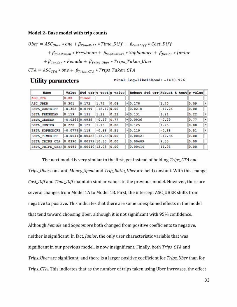
Model 2-‐ Base model with trip counts



+ 𝛽!"#$!" ∗ 𝐹𝑒𝑚𝑎𝑙𝑒 + 𝛽!"#$%_!"#$ ∗ 𝑇𝑟𝑖𝑝𝑠_𝑇𝑎𝑘𝑒𝑛_𝑈𝑏𝑒𝑟

𝐶𝑇𝐴 = 𝐴𝑆𝐶!"# ∗ 𝑜𝑛𝑒 + 𝛽!"#$%_!"# ∗ 𝑇𝑟𝑖𝑝𝑠_𝑇𝑎𝑘𝑒𝑛_𝐶𝑇𝐴

The next model is very similar to the first, yet instead of holding Trips_CTA and

Trips_Uber constant, Money_Spent and Trip_Ratio_Uber are held constant. With this change,

Cost_Diff and Time_Diff maintain similar values to the previous model. However, there are

several changes from Model 1A to Model 1B. First, the intercept ASC_UBER shifts from

negative to positive. This indicates that there are some unexplained effects in the model

that tend toward choosing Uber, although it is not significant with 95% confidence.

Although Female and Sophomore both changed from positive coefficients to negative,

neither is significant. In fact, Junior, the only user characteristic variable that was

significant in our previous model, is now insignificant. Finally, both Trips_CTA and

Trips_Uber are significant, and there is a larger positive coefficient for Trips_Uber than for

Trips_CTA. This indicates that as the number of trips taken using Uber increases, the effect

34

is stronger on utility than if the number of trips taken using the CTA increases. Overall, this

model has a much smaller log-‐likelihood than that of Model 1A, so Model 1A will continue

to be used in subsequent analyses.

35

Model 3-‐ Base model with time separated by mode 𝑈𝑏𝑒𝑟 = 𝐴𝑆𝐶!"#$ ∗ 𝑜𝑛𝑒 + 𝛽!"#$_!"#$ ∗ 𝑇𝑖𝑚𝑒_𝑈𝑏𝑒𝑟 + 𝛽!"#$%&'' ∗ 𝐶𝑜𝑠𝑡_𝐷𝑖𝑓𝑓



+ 𝛽!"#$_!"#$%_!"#$ ∗ 𝑇𝑟𝑖𝑝_𝑅𝑎𝑡𝑖𝑜_𝑈𝑏𝑒𝑟

𝐶𝑇𝐴 = 𝐴𝑆𝐶!"# ∗ 𝑜𝑛𝑒 + 𝛽!"#$_!"# ∗ 𝑇𝑖𝑚𝑒_𝐶𝑇𝐴

From here, the time variables were separated from the base model. The model could

not be specified with the Cost_CTA variable, as it did not vary in the model, so the cost

difference between the two modes is modeled instead. The coefficients of both time

variables are negative. This satisfied my hypothesis; as the length of a ride on each mode

increases, users are less likely to take that mode. Further, both time variables are highly

significant. One curious revelation from this model is that the coefficient of Time_Uber is

1.68 times that of Time_CTA. This can have several explanations. First, because an

additional ten minutes in an Uber can mean an additional $5, users are reluctant to choose

Uber. With the CTA, however, the cost does not change as time changes. This decision

works the opposite way as well; if a rider were to save ten minutes on an Uber ride, it

36

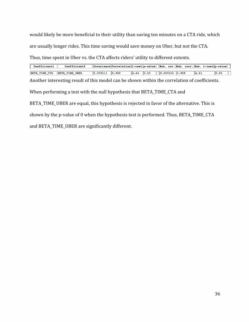
would likely be more beneficial to their utility than saving ten minutes on a CTA ride, which

are usually longer rides. This time saving would save money on Uber, but not the CTA.

Thus, time spent in Uber vs. the CTA affects riders’ utility to different extents.

Another interesting result of this model can be shown within the correlation of coefficients.

When performing a test with the null hypothesis that BETA_TIME_CTA and

BETA_TIME_UBER are equal, this hypothesis is rejected in favor of the alternative. This is

shown by the p-‐value of 0 when the hypothesis test is performed. Thus, BETA_TIME_CTA

and BETA_TIME_UBER are significantly different.

37

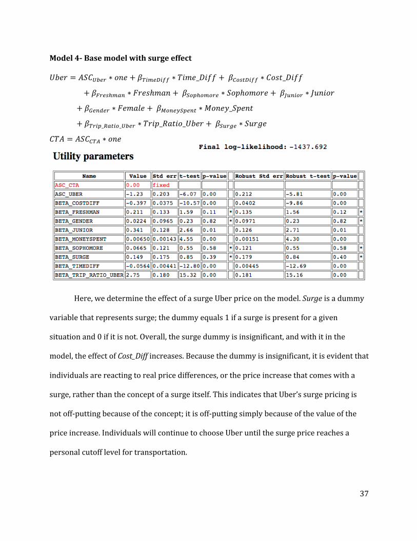
Model 4-‐ Base model with surge effect



+ 𝛽!"#$!" ∗ 𝐹𝑒𝑚𝑎𝑙𝑒 + 𝛽!"#$%&'$#( ∗𝑀𝑜𝑛𝑒𝑦_𝑆𝑝𝑒𝑛𝑡

+ 𝛽!"#$_!"#$%_!"#$ ∗ 𝑇𝑟𝑖𝑝_𝑅𝑎𝑡𝑖𝑜_𝑈𝑏𝑒𝑟 + 𝛽!"#$% ∗ 𝑆𝑢𝑟𝑔𝑒


Here, we determine the effect of a surge Uber price on the model. Surge is a dummy

variable that represents surge; the dummy equals 1 if a surge is present for a given

situation and 0 if it is not. Overall, the surge dummy is insignificant, and with it in the

model, the effect of Cost_Diff increases. Because the dummy is insignificant, it is evident that

individuals are reacting to real price differences, or the price increase that comes with a

surge, rather than the concept of a surge itself. This indicates that Uber’s surge pricing is

not off-‐putting because of the concept; it is off-‐putting simply because of the value of the

price increase. Individuals will continue to choose Uber until the surge price reaches a

personal cutoff level for transportation.

38

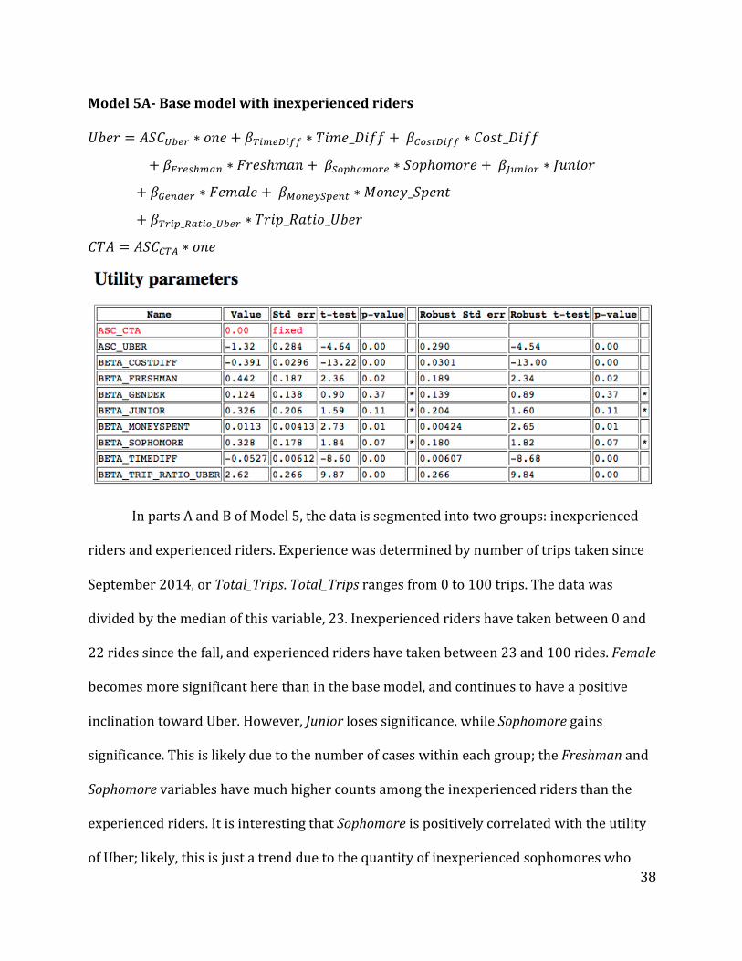
Model 5A-‐ Base model with inexperienced riders



+ 𝛽!"#$!" ∗ 𝐹𝑒𝑚𝑎𝑙𝑒 + 𝛽!"#$%&'$#( ∗𝑀𝑜𝑛𝑒𝑦_𝑆𝑝𝑒𝑛𝑡

+ 𝛽!"#$_!"#$%_!"#$ ∗ 𝑇𝑟𝑖𝑝_𝑅𝑎𝑡𝑖𝑜_𝑈𝑏𝑒𝑟


In parts A and B of Model 5, the data is segmented into two groups: inexperienced

riders and experienced riders. Experience was determined by number of trips taken since

September 2014, or Total_Trips. Total_Trips ranges from 0 to 100 trips. The data was

divided by the median of this variable, 23. Inexperienced riders have taken between 0 and

22 rides since the fall, and experienced riders have taken between 23 and 100 rides. Female

becomes more significant here than in the base model, and continues to have a positive

inclination toward Uber. However, Junior loses significance, while Sophomore gains

significance. This is likely due to the number of cases within each group; the Freshman and

Sophomore variables have much higher counts among the inexperienced riders than the

experienced riders. It is interesting that Sophomore is positively correlated with the utility

of Uber; likely, this is just a trend due to the quantity of inexperienced sophomores who

39

completed the survey. Cost_Diff, Time_Diff, Trip_Ratio_Uber and Money_Spent remain

significant.

40

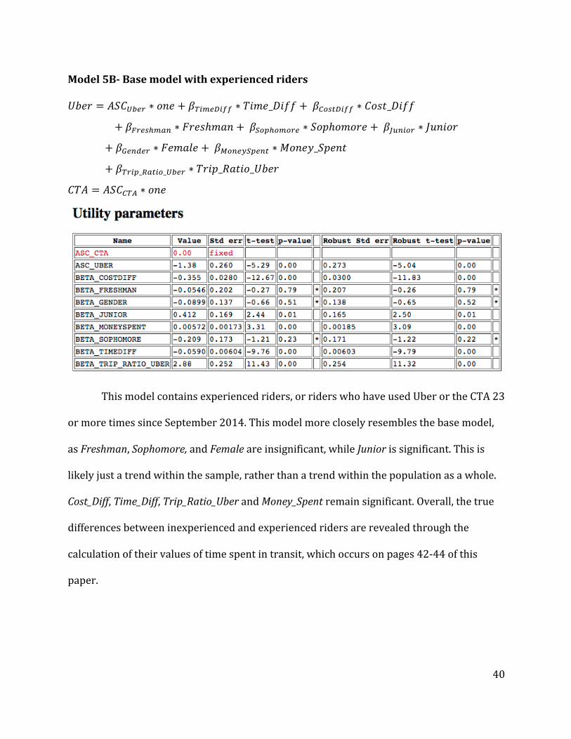
Model 5B-‐ Base model with experienced riders




+ 𝛽!"#$_!"#$%_!"#$ ∗ 𝑇𝑟𝑖𝑝_𝑅𝑎𝑡𝑖𝑜_𝑈𝑏𝑒𝑟


This model contains experienced riders, or riders who have used Uber or the CTA 23

or more times since September 2014. This model more closely resembles the base model,

as Freshman, Sophomore, and Female are insignificant, while Junior is significant. This is

likely just a trend within the sample, rather than a trend within the population as a whole.

Cost_Diff, Time_Diff, Trip_Ratio_Uber and Money_Spent remain significant. Overall, the true

differences between inexperienced and experienced riders are revealed through the

calculation of their values of time spent in transit, which occurs on pages 42-‐44 of this

paper.

41

Log-‐Likelihood Comparison

The final log-‐likelihood value when modeling solely the intercepts in the model,

with no explanatory variables, is -‐1841.606. With Model 1A, the best model found after

many iterations, this value is equal to -‐1438.056. Thus, when performing a log-‐likelihood

test, -‐1438.056 is subtracted from -‐1841.606 and the difference is multiplied by -‐2, giving

us a value of 807.1. To determine the degrees of freedom, the number of parameters in the

model with no explanatory variables (0) is subtracted from the number of parameters in

Model 1A (8), to find 8 degrees of freedom. These values are compared to a chi-‐square

distribution. In looking at the distribution, it is evident that 807.1 is greater than 15.507, so

the test passes with 95% certainty.

42

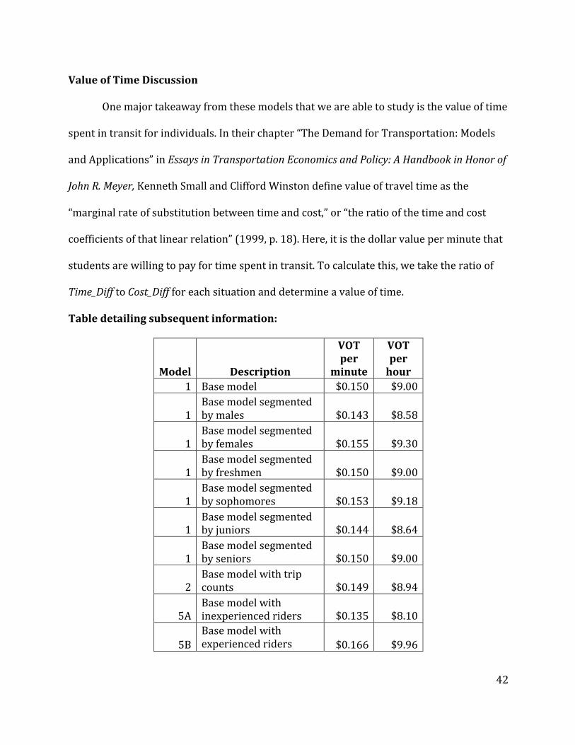
Value of Time Discussion

One major takeaway from these models that we are able to study is the value of time

spent in transit for individuals. In their chapter “The Demand for Transportation: Models

and Applications” in Essays in Transportation Economics and Policy: A Handbook in Honor of

John R. Meyer, Kenneth Small and Clifford Winston define value of travel time as the

“marginal rate of substitution between time and cost,” or “the ratio of the time and cost

coefficients of that linear relation” (1999, p. 18). Here, it is the dollar value per minute that

students are willing to pay for time spent in transit. To calculate this, we take the ratio of

Time_Diff to Cost_Diff for each situation and determine a value of time.

Table detailing subsequent information:

Model Description

VOT per

minute

VOT per hour

1 Base model $0.150 $9.00

1 Base model segmented by males $0.143 $8.58

1 Base model segmented by females $0.155 $9.30

1 Base model segmented by freshmen $0.150 $9.00

1 Base model segmented by sophomores $0.153 $9.18

1 Base model segmented by juniors $0.144 $8.64

1 Base model segmented by seniors $0.150 $9.00

2 Base model with trip counts $0.149 $8.94

5A Base model with inexperienced riders $0.135 $8.10

5B Base model with experienced riders $0.166 $9.96

43

Model 1-‐ Base model:

VOT: -‐0.0556/-‐0.370 = $0.150

In these models, the value of time represents a utility comparison of dollar to

minute, as the output of each model is the utility of Uber or CTA. Thus, for the above

example, if the cost difference increases by $1, the utility of Uber decreases by 0.0556 units.

If the time difference increases by 1 minute, the utility of Uber decreases by 0.370 units.

This estimation for value of time effectively translates minutes into dollars.

Moreover, this value is an extremely important finding. First of all, it demonstrates

that a Northwestern student’s average value of time spent in transit is $0.15 per minute, or

$9.00 per hour. This rate is close to the Chicago minimum wage rate, $8.25 per hour

(Lobosco, 2014). This value is helpful for transportation services that wish to price their

services at a desirable value.

From the base model, I made several variations to determine the value of time

among smaller subsets of our sample by partitioning the sample. To do this, I ran the same

model on the sample but instructed the model to solely include the desirable data. For

instance, I ran one model including exclusively men and one including exclusively women.

For men, the VOT is $0.143 per minute, while for women it is $0.155. While this difference

may not seem large, over an hour, the values rise to $8.58 and $9.30, respectively. This

result is interesting; it would seem that women value their time more highly than men, an

important finding in determining how Uber can better market to these groups. One

hypothesis regarding this occurrence is that women may feel unsafe when riding the CTA

alone, so they are willing to pay more for Uber to gain a feeling of security. However, this

finding may not be significant; because this is a small sample, there may be some

44

unexplained variation that does not ring true for the population. More work must be done

to determine further motivation behind this difference.

Furthermore, the value of time also varies by year in school. When partitioning the

data by year, I found the value of time for these sub groups. For freshmen, the VOT is

$0.150 per minute; for sophomores, it is $0.153 per minute; for juniors, it is $0.144 per

minute; and for seniors, it is $0.150 per minute. Clearly, there is no distinct pattern in this

variation, as I mentioned in my model analysis. This finding indicates that value of time has

no trend by year in school. More analysis must be done to search for further trends in this

realm.

Model 2-‐ Base model with trip counts:

VOT: -‐0.0541/-‐0.362 = $0.149

The value of time in Model 1B is strikingly similar to that of Model 1A, indicating

that although some variables differed slightly between the models, both are viable options

for determining the value of time spent in transit among individuals.

Model 5A-‐ Base model with inexperienced riders

VOT: -‐0.0527/-‐0.391 = $0.135

The value of time for inexperienced riders is lower than the overall value of time. On

a per hour basis, inexperienced riders value time at $8.10 per hour, in comparison to the

base value of $9.00 per hour. This is a noteworthy finding. This indicates that as users

become more familiar with transit modes, they will be more likely to pay more for trips and

value their time more highly.

Model 5B-‐ Base model with experienced riders

VOT: -‐0.0590/-‐0.355 = $0.166

45

The value of time for experienced riders is higher than the overall value of time, and

significantly higher than the value for inexperienced riders. On a per hour basis,

experienced riders value time at $9.96 per hour, which is much higher than the

inexperienced value of $8.10 per hour. Uber could use this information to target

experienced riders and encourage them to continue traveling with Uber. This shows that

the value of time climbs sharply with experience, and that past behavior is a strong

determinant of future behavior.

46

Conclusion and Limitations

Overall, the analysis presented returned some very interesting results. I determined

that an individual’s time spent in transit is $0.15 per minute. On an hourly basis, this value

of time is $9.00. The value jumps to $0.17 per minute among experienced riders, and also

varies by gender and year in school. This information sheds some light on individual

transportation behavior. I also found that overall, year in school and gender are not

significant in determining individual travel behavior, although the value of time varies

among these groups. Finally, I found that influential variables in determining an

individual’s mode choice are the ratio of trips taken in the past and average amount of

money spent on transit. This indicates that past behavior is highly influential in future

decisions.

This study had many limitations. First of all, by not varying CTA time, I entirely lost

the ability to assess the cost variables for each mode separately. This decision was made to

ensure that the time and cost values presented were accurate to those seen in the real

world. Another limiting decision was choosing to ask about money spent on transit, rather

than polling participants about total income. This choice was made for surveying purposes,

and to encourage users to be honest; income questions can incite deceit. However, money

spent on transit may not be an accurate substitute for total income, so this decision could

have been harmful to the results. Another decision that potentially hampered my results

was asking very few demographic questions. This was made in order to encourage

individuals to complete my survey; lengthy surveys can dishearten those who wish to take

them. As a potential result, the response rate was very large, but this came at the cost of

many additional survey background questions. Finally, the last limiting choice was the

47

sample; rather than attempting to get data from individuals across the Chicagoland region,

I surveyed solely Northwestern students. This was done for convenience.

Overall, the study went very well, and the results are quite strong. Future research

would involve a larger sample size and more specific user characteristic questions, such as

those used in Daniel McFadden’s study. Regardless of the specific results, this study shows

the enormous impact Uber has had on the transportation market as a whole.

48

Works Cited

Ali, R. (2015, April 30). Skift Survey: Younger Millennials Use Uber-‐Type Apps More Than

Older Millennials. Skift. Retrieved June 8, 2015, from

http://skift.com/2015/04/30/skift-‐survey-‐younger-‐millennials-‐using-‐uber-‐type-‐

apps-‐more-‐than-‐older-‐millennials/

CTA Facts at a Glance. (n.d.). Chicago Transit Authority. Retrieved June 8, 2015, from

http://www.transitchicago.com/about/facts.aspx

Dallke, J. (2015, January 20). How Much do Uber Drivers Make in Chicago? Study Looks at

Uber Pay Across the Country. Chicago Inno. Retrieved June 8, 2015, from

http://chicagoinno.streetwise.co/2015/01/22/uber-‐driver-‐pay-‐how-‐much-‐to-‐

chicago-‐uberx-‐drivers-‐make/

Lawler, R. (2015, January 22). Uber Study Shows Its Drivers Make More Per Hour And

Work Fewer Hours Than Taxi Drivers. TechCrunch. Retrieved June 8, 2015 from

http://techcrunch.com/2015/01/22/uber-‐study/

Lobosco, K. (2014, December 2). Chicago hikes minimum wage to $13. CNN Money.

Retrieved June 8, 2015, from

http://money.cnn.com/2014/12/02/news/economy/chicago-‐minimum-‐wage-‐

hike/

MacMillan, D. (2015, January 29). Uber Laws: A Primer on Ridesharing Regulations. Digits:

Tech News and Analysis from the WSJ. Retrieved June 8, 2015, from

http://blogs.wsj.com/digits/2015/01/29/uber-‐laws-‐a-‐primer-‐on-‐ridesharing-‐

regulations/

49

Madhani, A. (2015, May 18). Once a sure bet, taxi medallions becoming unsellable. USA

Today. Retrieved June 8, 2015, from

http://www.usatoday.com/story/news/2015/05/17/taxi-‐medallion-‐values-‐

decline-‐uber-‐rideshare/27314735/

McFadden, D. L. (1987). The Theory and Practice of Disaggregate Demand Forecasting for

Various Modes of Urban Transportation. In W. F. Brown, R. B. Dial, D. S. Gendell, & E.

Weiner (Eds.), Emerging Transportation Planning Methods. U.S. Department of

Transportation: Washington, D.C.

Neff, J. & Pham, L. (2007). A Profile of Public Transportation Passenger Demographics and

Travel Characteristics Reported in On-‐Board Surveys. American Public

Transportation Association. Retrieved June 8, 2015, from

http://www.apta.com/resources/statistics/Documents/transit_passenger_characte

ristics_text_5_29_2007.pdf

Newcomer, E. (2015, May 9). Uber Said to Seek $1.5 Billion in Funds at $50 Billion

Valuation. Bloomberg. Retrieved June 8, 2015, from

http://www.bloomberg.com/news/articles/2015-‐05-‐09/uber-‐said-‐to-‐seek-‐1-‐5-‐

billion-‐in-‐funds-‐at-‐50-‐billion-‐valuation

Ortúzar, J. & Willumsen, L. G. (2011). Modelling Transport (4th Edition). John Wiley & Sons,

Ltd: Chichester.

Rao, L. (2010, July 5). UberCab Takes The Hassle Out Of Booking A Car Service. TechCrunch.

Retrieved June 8, 2015, from http://techcrunch.com/2010/07/05/ubercab-‐takes-‐

the-‐hassle-‐out-‐of-‐booking-‐a-‐car-‐service/

50

Rao, L. (2011, September 20). Uber Brings Its Disruptive Car Service To Chicago.

TechCrunch. Retrieved June 8, 2015, from

http://techcrunch.com/2011/09/22/uber-‐brings-‐its-‐disruptive-‐car-‐service-‐to-‐

chicago/

Savage, I. (2014). Disaggregate Demand Models. Transportation Economics and Public

Policy. Department of Economics, Northwestern University, Evanston, IL.

Shontell, A. (2014, November 25). Is This The Highest Surge Price Ever Recorded In Uber

History? Business Insider. Retrieved June 8, 2015, from

http://www.businessinsider.com/ubers-‐highest-‐surge-‐price-‐ever-‐may-‐be-‐50x-‐

2014-‐11

Silverstein, S. (2014, October 16). These Animated Charts Tell You Everything About Uber

Prices In 21 Cities. Business Insider. Retrieved June 8, 2015, from

http://www.businessinsider.com/uber-‐vs-‐taxi-‐pricing-‐by-‐city-‐2014-‐10

Small, K. A. & Winston, C. (1999). The Demand for Transportation: Models and

Applications. In J. A. Gomez-‐Ibanez, W. B. Tye, & C. Winston (Eds.), Essays in

Transportation Economics and Policy: A Handbook in Honor of John R. Meyer (pp. 11-‐

56). London: Brookings Institution Press.

Smith, N. (2014, December 31). Here's What Economics Gets Right. Bloomberg View.

Retrieved June 8, 2015, from http://www.bloombergview.com/articles/2014-‐12-‐

31/heres-‐what-‐economics-‐gets-‐right

Smith IV, J. (2015, February 3). Uber Drivers: The Punishment For Bad Ratings Is Costly

Training Courses. Observer. Retrieved June 8, 2015, from

51

http://observer.com/2015/02/uber-‐drivers-‐the-‐punishment-‐for-‐bad-‐ratings-‐is-‐

costly-‐training-‐courses/

Train, K. E. (2009). Discrete Choice Methods With Simulation. New York: Cambridge

University Press.

Uber. (2014, December 29). Dynamic Pricing 101 | Uber. YouTube. Retrieved June 8, 2015,

from https://www.youtube.com/watch?v=76q7PDnxWuE