Embed Size (px)
Citation preview
Journal of Monetary Economics 32 (1993) 513-542. North-Holland
Finance, entrepreneurship, and growth
Theory and evidence*
Robert G. King University of Virginia, Charlottesville. VA 22901, USA Federal Reserve Bank of Richmond, Richmond, VA 23261, USA
Ross Levine The World Bank, Washingron, DC 20433, USA
Received March 1993, final revision received September 1993
How do financial systems affect economic growth? We construct an endogenous growth model in which financial systems evaluate prospective entrepreneurs, mobilize savings to finance the most promising productivity-enhancing activities, diversify the risks associated with these innovative activities, and reveal the expected profits from engaging in innovation rather than the production of existing goods using existing methods. Better financial systems improve the probability of successful innovation and thereby accelerate economic growth. Similarly, financial sector distortions reduce the rate of economic growth by reducing the rate of innovation. A broad battery of evidence suggests that financial systems are important for productivity growth and economic development.
Key words: Financial markets; Economic development
JEL classification: 01; 03
1. Introduction
A prominent feature of the recent literature on economic growth is a renewed interest in the links between financial systems and the pace of economic develop- ment. On the theoretical side, a new battery of models articulates mechanisms
Correspondence to: Robert G. King, Department of Economics, University of Virginia, Rouss Hall 116, Charlottesville, VA 22901, USA.
*This research was supported by the World Bank project ‘How Do National Policies Affect Long Run Growth?. We thank Marianne Baxter, Joydeep Bhattacharya, Gerard Caprio, Bill Easterly, Alan Gelb, Ronald McKinnon, Paul Romer, Steve Saeger and Mark Watson for helpful comments. Sara Zervos provided excellent research assistance.
0304-3932/93/SO6.00 0 1993-Elsevier Science Publishers B.V. All rights reserved
514 R.G. King and R. Levine, Finance, entrepreneurship, and growth
by which the financial system may affect long-run growth, stressing that finan- cial markets enable small savers to pool funds, that these markets allocate investment to the highest return use, and that financial intermediaries partially overcome problems of adverse selection in credit markets.’ On the empirical side, researchers have shown that a range of financial indicators are robustly positively correlated with economic growth.’ Increasingly, economists are thus entertaining the idea that government policies toward financial institutions have an important causal effect on long-run economic growth.
In traditional development economics, there were two schools of thought with sharply differing perspectives on the potential importance of finance. Econo- mists like Goldsmith (1969), McKinnon (1973), and Shaw (1973) saw financial markets as playing a key role in economic activity. In their view, differences in the quantity and quality of services provided by financial institutions could partly explain why countries grew at different rates. But many more economists accepted Robinson’s (1952) view that finance was essentially the handmaiden to industry, responding passively to other factors that produced cross-country differences in growth.3 In part, this skeptical view also derived from the mechan- ics of the neoclassical growth model: many believed that financial systems had only minor effects on the rate of investment in physical capital, and changes in investment were viewed as having only minor effects on economic growth as a result of Solow’s (1956, 1957) analyses.
In this paper, we develop an endogenous growth model featuring connections between finance, entrepreneurship, and economic growth suggested by the insights of Frank Knight (1951) and Joseph Schumpeter (1912). We combine the Knightian role of entrepreneurs in initiating economic activities with two ideas of Schumpeter. First, we build on the well-known Schumpeterian view that innovations are induced by a search for temporary monopoly profits.4 Second, we incorporate the less well-known Schumpeterian idea that financial institu- tions are important because they evaluate and finance entrepreneurs in their initiation of innovative activity and the bringing of new products to market.’
‘Recent theoretical studies include Bencivenga and Smith (1991) Boyd and Smith (1992). Green- wood and Jovanovic (1990), Levine (1991), and Saint-Paul (1992). Pagan0 (1993) provides an overview of the recent literature; Greenwood and Smith (1993) provide a detailed survey.
‘Recent empirical studies include Degregorio and Giudotti (1992). Gelb (1989), Gertler and Rose (1991), King and Levine (1993a, b), and Roubini and Sala-i-Martin (1992). See also The World Development Report (1989).
3Robinson’s skepticism about the importance of financial factors for growth is echoed in more recent articles by Lucas (1988) and Stern (1989).
“Recent general equilibrium frameworks embed Schumpeterian ideas of ‘creative destruction’, following Shleiffer (1986). Our model is in the class of endogenous growth models developed by Aghion and Howitt (1992), Grossman and Helpman (1991), and Romer (1990).
sWe take a broad view of innovative activity: in addition to invention of new products, we include enhancement of existing products; costly adoption of technology from other countries; and produc- tion of an existing good using new production or business methods.
R.G. King and R. Levine, Finanre. entrepreneurship, and growth 515
Like Schumpeter, we believe the nexus of finance and innovation is thus central to the process of economic growth.
At the center of our theory is the endogenous determination of productivity growth, which is taken to be the result of rational investment decisions. Produc- tivity growth is thus influenced by standard consideration of costs and benefits. In our analysis, financial systems influence decisions to invest in productivity- enhancing activities through two mechanisms: they evaluate prospective entre- preneurs and they fund the most promising ones. Financial institutions can provide these research, evaluative, and monitoring services more effectively and less expen,Gvely than individual investors; they also are better at mobilizing and providing appropriate financing to entrepreneurs than individuals. Overall, the evaluation and sorting of entrepreneurs lowers the cost of investing in produc- tivity enhancement and stimulates economic growth. Financial sector distor- tions can therefore reduce the rate of economic growth.
Our view of the relevant economic mechanisms is consequently quite different from existing theories, new and old. First, in contrast to traditional development work, we do not require that financial institutions mainly exert influence via the rate of physical capital accumulation.6 Second, distinct from recent theoretical research, we stress that financial institutions play an active role in evaluating, managing, and funding the entrepreneurial activity that leads to productivity growth. Indeed, we believe our mechanism is the channel by which finance must have its dominant effect, due to the central role of productivity growth in development, as shown in King and Levine (1993~).
With this theoretical model as background, we then present various types of evidence on the links between financial institutions and economic development. We begin by reviewing the cross-country evidence on links between financial indicators and economic growth, discussing key results from our earlier work in this area and undertaking some extensions. Next, we discuss three sets of evidence about the relationship between financial institutions and public policy interventions. First, we look at a number of case studies of how financial indicators have responded to government interventions designed to liberalize financial markets. Second, we review recent firm-level studies of the effects of financial sector reforms in two developing countries. Third, we look at how financial development has been related to the success of World Bank structural adjustment lending programs. Taken together, these diverse types of evidence support the view that the services of financial systems are important for produc- tivity growth and economic development.
The organization of the paper is as follows. In section 2, we articulate our theory of the links between finance and growth. In section 3, we review a range of evidence on financial institutions and economic growth.
60~r formal model takes this view to an extreme since it abstracts entirely from the mechanics of physical capital formation.
516 R.G. King and R. Levine. Finance, entrepreneurship, and growth
2. Theoretical linkages between financial markets and growth
In this section, we develop a theoretical model of the links between finance, entrepreneurship, and economic growth. We begin by modeling the process by which financial systems - financial intermediaries and securities markets - au- thorize particular entrepreneurs to undertake innovative activity. Next, we develop links between innovation and growth. Finally, we determine the general equilibrium of our economy and evaluate the effects of financial sector policies on economic growth.
To study the links between finance and innovative activity, we construct a basic model that highlights the demand for four services of the financial system. First, as in Boyd and Prescott (1986), investment projects must be evaluated to identify promising ones [on this process, see also Diamond (1984)]. Specifically, there are large fixed costs of evaluating the projects of prospective entrepreneurs, so that there are incentives for specialized organizations to arise and to perform this task. Second, the required scale of projects necessitates substantial pooling of funds from many small savers, so that it is important for financial systems to mobilize sufficient resources for projects. Third, the outcomes of attempts to innovate are uncertain, so that it is desirable for the financial system to provide a means for individuals and entrepreneurs to diversify these risks. Fourth, productivity en- hancement requires that individuals choose to engage in risk innovative activities rather than produce existing goods using existing methods. Since the expected rewards to innovation are the stream of profits which accrue from being an industry’s productivity leader, it is important for the financial system to accurately reveal the expected discounted value of these profits. Thus, the model generates a demand for four financial services: evaluating entrepreneurs, pooling resources, diversifying risk, and valuing the expected profits from innovative activities. But the model does not focus on the precise form of contracts and institutions that provide these services.
In practice, financial intermediaries commonly evaluate investment projects, mobilize resources to finance promising ones, and facilitate risk management: they thereby provide three of the services highlighted in our model. Thus, in this paper, we assume that these services are provided by integrated organizations which we call financial intermediaries. ’ For most of the discussion, we also assume that a stock market reveals the expected discounted value of profits from engaging in innovative activities.
‘We believe that evaluation, mobilization, and risk diversification are frequently bundled together as activities of a single financial intermediary because evaluation yields information, previously unknown by both evaluator and entrepreneur, which has important proprietary value. Bhattacharya (1992) discusses aspects of the optimal structure of financial intermediaries in settings with proprietary information.
R.G. King and R. Levine, Finance, entrepreneurship, and growth 517
In modeling the links between innovation and economic growth, we draw upon the basic theory of endogenous technical change developed by Aghion and Howitt (1992), Grossman and Helpman (1991), and Romer (1990). Our specific version of this theory involves innovations which permit a specific entrepreneur to produce one of many intermediate products at a cost temporarily lower than that of his rivals. The extent of innovative activity undertaken by society dictates the rate of economic growth.
In focusing attention on the nexus of finance, entrepreneurship, and innova- tion, our model thus stresses that the financial system is a lubricant for the main engine of growth. Better financial services expand the scope and improve the efficiency of innovative activity; they thereby accelerate economic growth. Financial repression, correspondingly, reduces the services provided by the financial system to savers, entrepreneurs, and producers; it thereby impedes innovative activity and slows economic growth.
Before presenting the model, it is worth noting that it describes financial intermediaries that mobilize external funds to finance innovative activity. One can, however, view innovative activity as containing two components: the costly act of creating a worthwhile innovation and the costly act of making this innovation operational on a market scale. Indeed, implementing a good innova- tion may be much more costly than undertaking experiments and pilot projects to identify and test the value of innovations. In this expanded setting, financial intermediaries might enter the productivity enhancement process only after an innovation has been identified, playing little role in the actual process of innovation. Yet, the efficiency of intermediaries would affect innovative activity, since the rewards to successful innovation depend on actually bringing new or improved products to market. Thus, even though intermediaries finance innova- tion directly in the model, the main results of the model should also apply to financial systems that participate only in the expansion to a market scale of new products and production methods.
2.1. A Schumpeterian model ofjnancial intermediation
Our theoretical framework contains the roles for financial intermediaries discussed above, specifically entrepreneurial selection and provision of external finance. We imagine an economy with many individuals. Each has N units of time as an endowment and has (equal) financial wealth, which is a claim to a diversified protfolio of claims on the profits of firms. Some individuals do have special capacity to manage innovative activity in the analysis, but this does not lead them to accumulate differing wealth levels.
518 R.G. King and R. Levine. Finance, entrepreneurship, and growth
2.1.1. Entrepreneurial selection
We assume that some individuals in society intrinsically possess the skills to be potentially capable entrepreneurs. Each potential entrepreneur has the endowment of a project and the skills to manage this project capably with probability a (otherwise the individual has no ability to manage a project). These capabilities are unknown to both the entrepreneur and intermediary. The actual capacity of an individual to manage a project can be ascertained at a cost of If’ units of labor input: by paying this cost, the evaluator learns whether the individual is either capable or not. (We assume that entrepreneurs cannot evaluate themselves and credibly communicate the results to others.) Thus, under some conditions that we detail below, there is an economic demand for a ‘rating’ activity that will sort potential entrepreneurs. If the market value of a ‘rated’ entrepreneur is ‘q’ and the wage rate is ‘w’, then competition among such organizations requires
aq = wfT
if there is to be positive output of this rating industry and, more generally, we must have aq I wf: That is, our entrepreneurial selection condition (1) requires the expected income from rating prospective entrepreneurs (aq) must equal the cost of that activity (wf).*
We treat evaluation activity as requiring only time units and assume that there are no shifts in the productivity of labor input. This assumption is convenient for our purposes in that it makes it easy to construct a steady state growth model. A useful extension to our analysis would be to model improve- ments in evaluation technology symmetrically with improvements in the tech- nology for making other products.
2.1.2. Financing of innovative activity
Each rated entrepreneur requires a total of x labor units (including his own time) to realize a marketable innovation with probability rr.9 This productive activity takes time: ‘x’ labor units must be invested prior to learning about success or failure of the innovative activity.
‘Throughout, we require that costly selection is an equilibrium outcome. We assume that the expected net savings in labor costs from evaluation exceed the labor costs of blind investment, or x>ax+j
91n the working paper version of this research, we permit the scale of the firm to be determined endogeneously, i.e., we make the innovation probability a function of scale, n(x). For some policy interventions of interest, including the tax distortion r studied below, the scale of the firm is invariant in equilibrium.
R.G. King and R. Levine, Finance, entrepreneurship, and growth 519
The value of a successful innovation is that the entrepreneur captures monop- oly profits. In the model developed below, this is the present value of profits earned by the current productivity leader (producing a specific intermediate product at lowest cost). As in Grossman and Helpman (1991), we call this reward the stock market value of the incumbent firm.
Under the technology described above, x units of labor input (with cost wx) must be invested at the start of the innovation process. The innovative activity has the expected reward 7fp,+A&,+Al, where P,+A~,~ is the discount factor at t for cash flows at t + At and Vt+& is the future stock market value of being an incumbent firm. For notational convenience, we write this as rcpv’, suppressing the time subscripts. Thus, the expected innovation rents to a rated individual innovation firm are given by npv’ - wx. If we add a tax at rate T on the gross income generated by a successful entrepreneur - the financial intermediary’s income stream from its earlier provision of external finance - then the value of a rated entrepreneur is given by the innovation rents specification as
q = (1 - z)npV - wx. (2)
If there is long-run constancy of the discount factor (p), the entrepreneurial selection (1) and innovation rents (2) conditions imply that q, w, and v must share common long-term growth rates.
External finance of innovative activity is a central element of the model for two reasons. First, the labor requirements of innovation are assumed to be much larger than just the entrepreneur’s time (i.e., x is much bigger than one). This makes it likely, though not certain, that the entrepreneur’s wealth would be insufficient to cover wage payments to the other members of his ‘firm’. Second, in the equilibrium studied below, the risk of innovation success is entirely diversifiable, so that reliance on any amount of internal finance is inefficient. Hence, the financing of innovative activity takes the form of a large intermediary providing the certain income streams to all members of an innovation team (including the entrepreneur).
2. I .3. Equilibrium jinancial intermediation
Combining the two equilibrium conditions for financial intermediation activity - entrepreneurial selection (1) and innovation rents (2) - we find that equilibrium in the jinancial intermediation sector requires
7Tpl.f = U(T)W, (3)
where the coefficient a(z) = (f/a + x)/(1 - r) reflects the combination of two
J.Mon- F
520 R.G. King and R. Levine, Finance, entrepreneurship. and growth
influences. First, the full labor requirement of an innovation project, a(O) = (f/a + x), includes evaluation resources per funded project (f/a) as well as direct labor requirements (x). Second, z includes both explicit financial sector taxes and implicit taxes arising from financial sector distortions.
2.1.4. Rational stock market valuations
Previously, we noted that an innovation at date t permits the innovator to capture a stream of rents equal in value to the stock market valuation of the incumbent monopolist. Correspondingly, such an innovation inflicts a capital loss on the stockholders of the currently dominant firm. These prospective capital losses are built into rational stock valuations.
Let v, denote the market value - prior to distribution of dividends 6, - of a representative incum~nt firm. In the general equilibrium constructs below, industries do not differ in the level of their leader’s stock price, so it is sufficient to consider a representative industry. Further, in the full model, each industry is small relative to (certain) aggregate wealth and, hence, the risk of capital losses due to a rival firm’s innovation success is diversiliable: securities are priced as if individuals were risk-neutral.
Hence, the equilib~um condition for holding a share of stock from t to t + At is
(1 - WP r+&fvt+dt = VI - 6,.
The left-hand side of (4) is the expected discounted value of the future stock value, taking into account the probability of capital losses; the right-hand side is the ‘ex dividend’ firm value. In this expression and below, the symbol l7 re- presents the probability that some entrepreneur will successfully innovate: for investors in a security, this is the relevant probability of a capital loss. Our assumption is that the probability of an innovation in a specific industry is simply proportional to the number of individual entrepreneurs seeking to im- prove that product, so that if there are ‘e’ participants, then n = 71e.i’
2.1.5. The stock market andfinancial intermediaries
In our model, stock markets play two roles. First, stock markets reveal the value of firms as determined by the analyses of rational investors. Second, stock
loThis is a standard assumption in growth models, but it is worth noting that it requires a ‘search coordination’ among the participants in the research process, which is discussed in more detail in our working paper.

R.G. King and R. Levine, Finance, entrepreneurship. and growth 521
markets provide a vehicle for pooling the risks of holding claims on established firms: on a balanced portfolio of all stocks, an investor gains a certain portfolio return.
Interpreting our model as that of a developed country, it is natural to view our financial intermediary as a venture capital firm, funding start-up innovative activity, in exchange for (most of) the firm’s stock. When the venture capital firm learns whether a specific entrepreneur has produced a marketable innovation or has not, it then sells off the shares on a stock market. However, as this interpretation makes clear, a formal stock exchange need not exist, although we do require that property rights be clearly defined and enforced. For example, the venture capital firm could be part of a larger financial conglomerate that provides the risk pooling and firm valuation which is given by the stock market in our model.
That is, our model identifies important financial services like project evalu- ation, resource mobilization, risk pooling, and valuation of risky cash flows; it does not focus on the precise form of contracts and institutions that provide these services. This is important since it indicates that the basic concepts in the model apply to countries with diverse financial systems.
2.2. A Schumpeterian model of technical progress
We now develop a Schumpeterian model of technical progress based on Grossman and Helpman (1991). Like those authors, we consider an economy with a continuum of products, indexed by w on the interval 0 I o I 1, which are subject to technical improvement. Each innovation moves a particular product’s technology one step up a ladder with steps j = 0, 1, . . . , realizing levels ,4j with ,4 > 1. Inventions are cost-reducing as in Aghion and Howitt (1992) and apply to an intermediate product as in Romer (1990). As in Grossman and Helpman (1991) the timing of individual innovations is random but the aggregate economy evolves deterministically.
2.2.1. Intermediate product technology
The production technology for the leading firm in industry o at ladder position j is yl(o) = A,(o)n,(o) = A%,(w), where y,(w) is physical output of intermediate product w, A,(o) is the level of productivity at date t in industry w, and n,(w) is the level of labor input. Thus, at wage rate w,, unit cost is w,n,(o)/y,(w) = w,/A,(w) = w,/Aj, i.e., unit cost is raised by wages and lowered by higher productivity.
522 R.G. King and R. Levine, Finance, entrepreneurship. and growth
2.2.2. Final goods production
The goods subject to technical innovation are assumed to be intermediate inputs into the production of a single final good, C. Letting z(o) be the quantity of input o demanded, the production technology for this good is C = exp(JA log(z(o))do), which is the continuum analog of the standard Cobb-Douglas production function with constant returns-to-scale imposed. Notice that the production function for the final good is time-invariant, so that all technical progress is embodied in intermediate products: this makes con- sumption a natural numeraire in our economy. Given that the price of inter- mediate product o is p,(o), factor demands are Z+(O) = C/p,(w), assuming the numeraire is consumption [so fh p(w)z(o)dw = 1 for C = 11.
2.2.3. Pricing of intermediate products
As in Grossman and Helpman (1991), we assume that there is a unique lead firm in industry w which prices its product at its rival’s unit costs, leading to a gross markup n over the lead firm’s unit cost, p, = nw,/A,(w). The producer of intermediate product o earns a stream of profits 6,(o) = p,(o)y&) - w,n,(o). Given the pricing rule, profits are simply a,@) = ~w*n~(~), with m = (A - 1) being the net markup. (We carry along this separate notation for the markup so that we may later see how it influences the nature of the growth process separately from the size of a productivity step, _4.) In product market equilib- rium, labor allocations are invariant across sectors, n,(o) = IZ~, which is a con- ventional result in CobbDouglas economies. Thus, profits in all sectors are identical, 6,(w) = nzw,n,.
For the general equilibrium analysis below, only a reduced form of the industry equilibrium given productivity is important. In particular, we carry along the finding that the profit flow is 6, = mw,n,: the present value of these profits is the reward to successful innovation.
2.2.4. Aggregate productivity growth
Our framework has a natural measure of the aggregate state of productivity, A, = exp(jA logtA,W)d o. This aggregate permits us, for example, to derive a reduced form ‘production function’ for final consumption goods as C, = Atn,, so that long-term consumption and productivity growth rates are equal. At the industry level, the dynamics of productivity are
A+&4 = A,(o)A with probability (II)dt A,(w) with probability (1 - II)& ’
(5)
R.G. King and R. Levine. Finance, entrepreneurship, and growth 523
for 0 I o I 1. For small time intervals, the aggregate then obeys dA,/dt = A,II& where 1= log(A) is the continuously compounded rate of productivity growth which occurs when innovation is certain in each industry (I7 = 1). More generally, our measure of the economy’s growth rate, y, is the common growth rate of consumption and the productivity aggregate. Since the innovation probability ZI is directly related to the number of entrepreneurs (or scale of labor input devoted innovation), I7 = rce, the growth rate is as well.”
2.3. General equilibrium
Our analysis of general equilibrium splits the problem into two parts. First, we discuss linkages between interest rates and growth rates that arise in market equilibrium on the side of production. Our framework enables us to describe how financial market distortions affect this tradeoff. Second, we discuss the implications of optimal choice of consumption over time for the preference- side relation between growth and returns. Then, we put these together in a general equilibrium analysis.
2.3.1. Production-side linkages between returns and growth
Three market equilibrium conditions determine the production-side relation- ship between growth and returns: the financial intermediation equilibrium conditions, the stock market equilibrium condition, and the labor market equilibrium condition.
Financial Equilibrium Conditions: The specific versions of the first two equi- librium conditions that we use are the relevant conditions for short periods (continuous time):
7ru, = a(7)w,, (3’)
dv,/dt = l7v, - S, + r*v,, (4’)
where r, is the instantaneous real interest rate prevailing between t and t + At, i.e., P~+~~,* = exp(r, At), and du,/dt is the time derivative of the stock price. As above, these conditions describe a representative industry. Moving to continu- ous time has some advantages in terms of the simplicity of results and their comparability to the literature, but comes at a cost of not having financial intermediary interest rates enter in the condition (3’).12
“Appendix B of our working paper considers the determination of optimal productivity growth using this aggregative framework.
12The limiting arguments used to construct the continuous time equations in this section are detailed in our working paper.

524 R.G. King and R. Levine. Finance, entrepreneurship. and growth
Labor Market Equilibrium: The labor market equilibrium condition is given by the requirement that
n + a(O)e = N, (6)
where n = 1: n(o)do is the total quantity of labor allocated to production of intermediates, a(O)e is the quantity of labor allocated to intermediation and innovation, and N is the total stock of available labor.
Stock Market and Growth: If the interest rate is constant, as it will be in the general equilibrium below, stock prices will grow with dividends (at the rate of productivity growth y). Imposing du,/dt = yu,, the stock market equilibrium condition may be written as
u = 6/(r - y + II). (7)
Treating r, 6, and II as fixed, this expression has the familiar implication that an increase in the growth rate raises the stock market value, since it increases the stream of future dividends. In our general equilibrium setting, this familiar result is tempered by two other considerations. First, when more resources are allocated to innovation and the economy consequently grows faster, there is a higher probability of successful innovation (a higher n), and therefore a higher probability that existing equity holders will suffer a capital loss. That is, since the growth rate y is given by HA, a higher innovation probability is associated with faster growth (for a given size of innovation A). Second, when more resources are allocated to innovation and the economy consequently grows faster, lower profits are earned by intermediate good producers since there is a smaller scale of their industries. These two considerations imply the full effect of the growth rate on the stock market is ambiguous.
The Production-Side Relation: Combining the financial intermediation, stock market, and labor market equilibrium conditions with the requirement that the aggregate innovation probability is Xl = ne and 6, = mw,n, we can determine a ‘production-side’ relationship between the growth rate and the real interest rate in the model’s steady state (which it is always in). Since the financial intermediation equilibrium condition (FI) is u = a(T)w, we can implicitly define a production-side relation:
a(z) = 71 S/W mn
r - [(A - l)/A]y = ’ r - [(A. - l)/A]y’ (8)
R.G. King and R. Levine. Finance, entrepreneurship, and growth 525
where 1 = log(n). Using Z7 = rre, n + a(O)e = N, and y = n1, (8) may be written as the line
(8’)
where 7 is the maximum feasible growth rate, defined by 7 = Nlrr/~(O).‘~ An implication of (8’) is that financial sector tax hikes lower the real return (r)
associated with any particular growth rate (y), which may be shown as follows. First, when the growth rate is at its maximum, y = 7, then the interest rate is r(y) = (1 - l/J) for all tax rates, so that changes in r rotate the (8’) locus through this point. Second, when growth is zero, y = 0, r(O) = (m/L)(l - T), so that an increase in financial sector taxation (r) lowers the intercept on the r axis. Hence, at any given y, there is an unambiguous inverse relationship between the real return, r, and the tax rate, z.
By contrast, the slope of the production-side relation is of ambiguous sign, which derives from the ambiguous long-run effect of growth on the stock market.
2.3.2. Preference-side linkages between returns and growth
We close our model by describing the saving behavior of an immortal family with a time-separable utility function, U, = j: u(c,+,)e-“ds, and a momentary utility function given by u(c,) = [c, (1-u) - l]/[i - a]. In this utility specification, there are two parameters which describe intertemporal preferences: the inter- temporal elasticity of substitution in consumption, l/o, and the pure rate of time preference, v.
The preference-side relationship between the real return and the growth rate is then given by
y = [r - VI/O. (9)
Hence, as stressed by Fisher (1930), there is a positive relationship between the rate of return and the growth rate; the strength of this relationship is determined by the intertemporal elasticity of substitution.
2.3.3. The equilibrium growth rate
The market equilibrium growth rate satisfies (8) and (9). Solving these equa- tions yields
y = [
; jr(l - 7) - v li[ o-I++++~(l-T). 1 (10)
13This growth rate obtains if all labor is allocated to innovative activity (including the screening of prospective entrepreneurs).
526 R.G. King and R. Levine, Finance, entrepreneurship, and growth
As in endogenous growth models with perfect competition, this market equilib- rium growth rate depends on aspects of preferences and technology. It is higher if individuals discount the future less (lower v) or are more willing to substitute through time (lower rr). The growth rate is also higher if the economy is more productive (in the sense of a higher maximum feasible growth rate 7). Reflecting the imperfect competition features of the model, growth depends positively on the extent of markups (m) and negatively on the extent of capital losses which innovation inflicts on investors (l/1).
2.4. The financial sector and economic growth
We now use our framework to study links between the financial sector and economic growth.
2.4.1. Growth efects ofJinancia1 sector distortions
Many financial sector policies effectively involve the taxation of gross income from financial intermediation and, thus, involve shifts in our parameter r hold- ing fixed the other parameters of the model. In practice, such financial taxes come in many forms. Charnley and Honohan (1990) discuss many examples of explicit financial sector taxes (including taxes on gross receipts of banks, value added taxes, taxes on loan balances, taxes on financial transactions, and taxes on intermediary profits). They also define and measure implicit or quasi- taxes on financial intermediaries (including non-interest-bearing reserve re- quirements, forced lending to the government and to state enterprises, and interest ceilings on various loans and deposits). Charnley and Honohan (1990) show that total financial intermediary taxation in some African countries amounted to 7 percent of the gross domestic product (GDP) during the 1980s. Similarly, Giovannini and de Melo (1993) find that financial intermediary taxes - especially implicit taxes - were above 2 percent of GDP for many countries.
Fig. 1 demonstrates the implications of increases in financial sector distor- tions - the explicit or implicit taxes captured by z - on the real return and the growth rate. (For concreteness, we have drawn the production-side relation as downward sloping, but this is inessential to the effects considered here.) In- creases in these taxes raise the full cost of innovation, a(z), shifting down the production-side relation. That is, the higher cost of evaluating and financing entrepreneurs means that there is a lower rate of return at any given growth rate. Hence, these interventions lead to a lower market equilibrium growth rate.
Our model can also be used to explore the growth effects of increases in the efficiency of the financial sector, such as a decrease in the time cost of evaluation
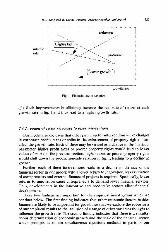
R.G. King and R. Levine, Finance, entrepreneurship. and growth 527
preferences
interest rate
growth rate
Fig. 1. Financial sector taxation.
(f). Such improvements in efficiency increase the real rate of return at each growth rate in fig. 1 and thus lead to a higher growth rate.
2.4.2. Financial sector responses to other interventions
Our model also indicates that other public sector interventions - like changes in corporate profits taxes or shifts in the enforcement of property rights - can affect the growth rate. Each of these may be viewed as a change in the ‘markup’ parameter: higher profit taxes or poorer property rights would lead to lower values of m. As in the previous section, higher taxes or poorer property rights would shift down the production-side relation in fig. 1, leading to a decline in growth.
Further, each of these interventions leads to a decline in the size of the financial sector in our model: with a lower return to innovation, less evaluation of entrepreneurs and external finance of projects is required. Specifically, lower returns to innovation cause entrepreneurs to demand fewer financial services. Thus, developments in the innovative and productive sectors affect financial development.
These two findings are important for the empirical investigation which we conduct below. The first finding indicates that other economic factors besides finance are likely to be important for growth, so that we explore the robustness of our empirical results to the inclusion of a range of other variables thought to influence the growth rate. The second finding indicates that there is a simulta- neous determination of economic growth and the scale of the financial sector, which prompts us to use simultaneous equations methods in parts of our
528 R.G. King and R. Levine, Finance, entrepreneurship. and growth
empirical work. Finally, the responsiveness of an economy to policy changes will depend on the how well its financial markets work.
3. Empirical linkages between financial markets and growth
We use four kinds of evidence to evaluate the theory’s predictions regarding the links between financial development and growth. First, we review and extend King and Levine’s (1993a) analysis of 80 countries over the 1960-1989 period (we subsequently refer to this earlier work as KL). Second, we evaluate five countries’ experiences with financial sector reforms. Third, we review firm- level evidence on the allocative effects of financial reforms. Finally, we investi- gate how success of general policy reforms depends on financial development.
The evidence from each empirical approach corresponds well with the theo- retical perspective developed above. The cross-country econometric results suggest that financial services are importantly linked to economic growth and productivity improvements. Further, the level of financial development predicts future economic growth and future productivity advances. The case studies indicate that the aggregate measures of financial development used in the broad cross-country analysis move in predictable ways, following identifiable financial policy reforms. This finding suggests a link between financial sector policies and long-run growth given the cross-country results. Moreover, firm-level studies indicate that financial liberalization tends to increase the funding of more efficient firms at the expense of less efficient firms. Further, after controlling for a variety of initial conditions, the initial level of financial development is positively associated with the beneficial effects of nonfinancial policy reforms. Finally, when nonfinancial policy changes are accompanied by financial reform, success tends to be even greater. Thus, the efficacy of other policy reforms depends on the financial system as suggested by our model.
3.1. Cross-country analysis ofjnancial development and economic growth
We begin by considering the cross-country relationship between various indicators of financial sector development and indicators of the pace of eco- nomic development.
3.1 .I. Indicators offinancial development and economic growth
In the model, financial intermediaries provide financial services: they evaluate prospective entrepreneurs, fund projects with relatively good chances of success, diversify risk, and value activities. To measure these financial services, we use four indicators of financial development constructed by KL. First, we use a measure of the overall size of the formal financial intermediary sector that
R.G. King and R. Levine, Finance, entrepreneurship, and growth 529
equals the ratio of liquid liabilities to GDP and call this variable DEPTH.14
Liquid liabilities equal currency held outside of the banking system plus demand and interest-bearing liabilities of banks and nonbank financial intermediaries. The assumption behind this measure is that the size of the financial sector is positively correlated with the provision of financial services.
Since DEPTH may not accurately reflect the provision of financial services, we try to isolate those financial intermediaries which are more likely to provide the services suggested by theory. Our second financial development indicator, BANK, equals the ratio of deposit money bank domestic assets to deposit money bank domestic assets plus central bank domestic assets. Banks seem more likely to provide the types of financial services emphasized in our model tan central banks, so that higher values of BANK should correspond to more financial services and higher levels of financial development. Although there are problems with BANK, banks are the main noncentral bank financial intermediary internationally, and BANK will augment the first financial development indicator, DEPTH.
A financial system which simply funnels resources to the public sector or state-owned enterprises is unlikely to be providing the types of financial services examined in the theoretical part of this paper. Thus, we design the third and fourth financial indicators to measure to whom the financial system is allocating credit. PRIVATE equals credit issued to private enterprises divided by credit issued to central and local governments plus credit issued to public and private enterprises. PRI V/ Y equals credit issued to private enterprises divided by GDP. Higher values of PRIVATE reflect a redistribution of credit from public enter- prises and government to private firms. Higher values of PRI V/Y indicate more credit to the private sector as a share of GDP. Thus, if financial sector interac- tions with the private sector are more indicative of the provision of productivity- enhancing financial services than financial sector interactions with the public sector, higher values of PRIVATE and PRI V/ Y should indicate greater finan- cial development. Along with DEPTH and BANK, PRIVATE and PRI V/Y
should help characterize the degree of financial development.” To examine the channels through which financial development may be linked
to long-run growth, we decompose real per capita GDP growth into two components: the rate of physical capital accumulation and everything else. Specifically, let y equal real per capita GDP, k equal the real per capita physical capital stock, x equal other determinants of per capita growth, and u is a pro- duction function parameter, so that y = k”x. Taking logarithms and differencing yields GYP = a(GK) + PROD, where GYP is the growth rate of real per capita GDP, GK is the growth rate of the real per capita physical capital stock, and
‘%ee King and Levine (1993a) for a description of the data sources.
“As in Gelb (1989), we also examined a measure of a very repressed interest rate - average real interest rates of less than -5 percent over extended time periods - but this indicator was not robustly linked to growth [see King and Levine (1992a)]. Table I provides summary statistics of these indicators.
530 R.G. King and R. Levine. Finance, entrepreneurship, and growth
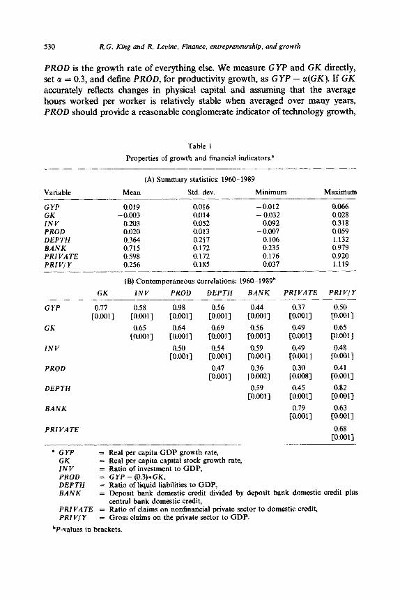
PROD is the growth rate of everything else. We measure GYP and GK directly, set CL = 0.3, and define PROD, for productivity growth, as GYP - c((GK). If GK accurately reflects changes in physical capital and adding that the average hours worked per worker is relatively stable when averaged over many years, PROD should provide a reasonable conglomerate indicator of technology growth,
Table 1
Properties of growth and financial indicators.’
Variable
(A) Summary statistics: 1960-1989
Mean Std. dev. Minimum Maximum
GYP GK INV PROD DEPTH BANK PRIVATE PRtVjY
GYP
GK
tNV
PROD
DEPTH
BANK
PRIVATE
0.019 0.016 -0.012 0.066 -0.003 0.014 - 0.032 0.028
0.203 0.052 0.092 0.318 0.020 0.013 -0.007 0.059 0.364 0.217 0.106 1.132 0.715 0.172 0,235 0.979 0.598 0.172 0.176 0.920 0.256 0.185 0.037 1.119
(B) Contemporaneous correlations: 1960-1989b
GK iNV PROD DEPTH BANK PRIVATE PRiVjY
0.77 0.58 0.98 0.56 0.44 0.37 0.50 [O.OOl] [O.OOl] [O.OOl] [0.001] [O.OOl] [O.OOl] [O.OOl]
0.65 0.64 0.69 0.56 0.49 0.65 [0.001] [0.001-J [O.oOi] [O.OOl] [0.001-j [O.OOl]
0.50 0.54 0.59 0.49 0.48 [0.001-J [O.OOl] [O.OOl] [O.OOl] [O.OOl]
0.47 0.36 0.30 0.41 [O.OOl] [0.002] [0.008-J [O.OOl]
0.59 0.45 0.82 [O.OOl] [O.OOl] [O.OOl]
0.79 0.63 [O.Ool] [O.OOl]
0.68 [O.OOl]
a GYP GK tNV PROD DEPTH BANK
PRIVATE PRIV/Y
bP-values in brackets.
central bank domestic credit, = Ratio of claims on nonfinancial private sector to domestic credit, = Gross claims on the private sector to GDP.
= Real per capita GDP growth rate, = Real per capita capital stock growth rate, = Ratio of investment to GDP, = G YP - (0.3)* GK, = Ratio of liquid liabilities to GDP, = Deposit bank domestic credit divided by deposit bank domestic credit plus
R.G. King and R. Levine, Finance, entrepreneurship, and growth 531
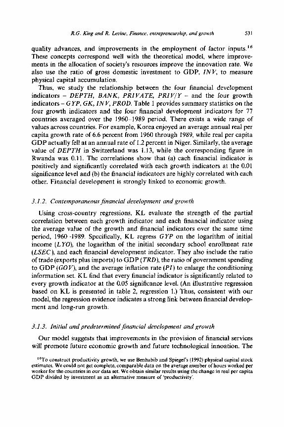
quality advances, and improvements in the employment of factor inputs.16 These concepts correspond well with the theoretical model, where improve- ments in the allocation of society’s resources improve the innovation rate. We also use the ratio of gross domestic investment to GDP, IN V, to measure physical capital accumulation.
Thus, we study the relationship between the four financial development indicators - DEPTH, BANK, PRIVATE, PRI V/Y - and the four growth indicators - G YP, GK, IN V, PROD. Table 1 provides summary statistics on the four growth indicators and the four financial development indicators for 77 countries averaged over the 1960-1989 period. There exists a wide range of values across countries. For example, Korea enjoyed an average annual real per capita growth rate of 6.6 percent from 1960 through 1989, while real per capita GDP actually fell at an annual rate of 1.2 percent in Niger. Similarly, the average value of DEPTH in Switzerland was 1.13, while the corresponding figure in Rwanda was 0.11. The correlations show that (a) each financial indicator is positively and significantly correlated with each growth indicators at the 0.01 significance level and (b) the financial indicators are highly correlated with each other. Financial development is strongly linked to economic growth.
3.1.2. ContemporaneousJinancial development and growth
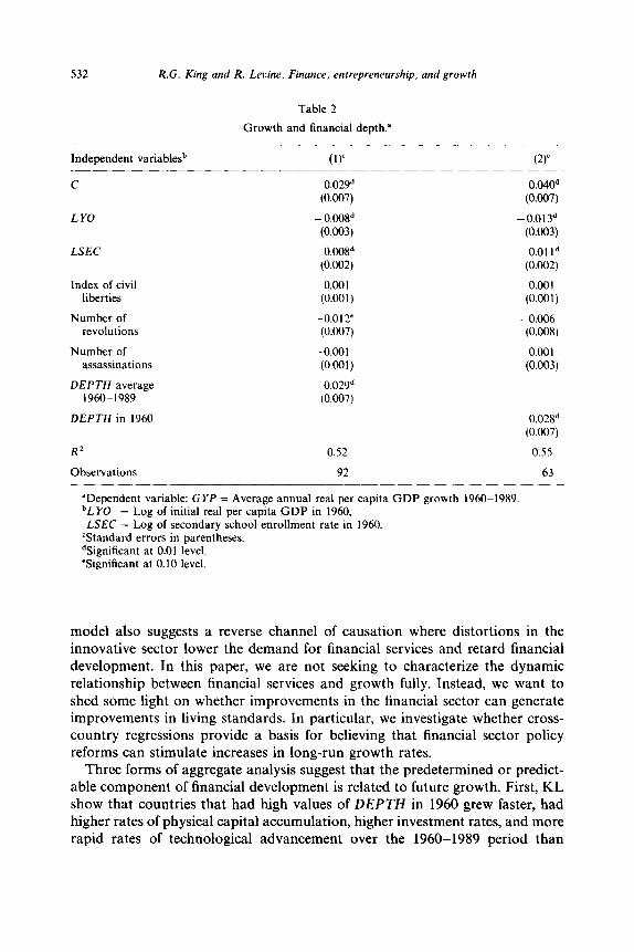
Using cross-country regressions, KL evaluate the strength of the partial correlation between each growth indicator and each financial indicator using the average value of the growth and financial indicators over the same time period, 1960-1989. Specifically, KL regress GYP on the logarithm of initial income (LYO), the logarithm of the initial secondary school enrollment rate (LSEC), and each financial development indicator. They also include the ratio of trade (exports plus imports) to GDP (TRD), the ratio of government spending to GDP (GOV), and the average inflation rate (PI) to enlarge the conditioning information set. KL find that every financial indicator is significantly related to every growth indicator at the 0.05 significance level. (An illustrative regression based on KL is presented in table 2, regression 1.) Thus, consistent with our model, the regression evidence indicates a strong link between financial develop- ment and long-run growth.
3.1.3. Initial and predetermined financial development and growth
Our model suggests that improvements in the provision of financial services will promote future economic growth and future technological innoation. The
l6To construct productivity growth, we use Benhabib and Spiegel’s (1992) physical capital stock estimates. We could not get complete, comparable data on the average number of hours worked per worker for the countries in our data set. We obtain similar results using the change in real per capita GDP divided by investment as an alternative measure of ‘productivity’.
532 R.G. King and R. Levine, Finance, entrepreneurship, and growth
Table 2
Growth and financial depth.”
Independent variablesb (1) (2)
c 0.029d 0.040d (0.007) (0.007)
LYO - 0.008d -0.013d (0.003) (0.003)
LSEC 0.008d 0.01 Id (0.002) (0.002)
Index of civil 0.001 0.001 liberties (0.001) (0.001)
Number of -0.012 - 0.006 revolutions (0.007) (0.008)
Number of -0.001 -0.001 assassinations (0.001) (0.003)
DEPTH average 0.029* 1960-1989 (0.007)
DEPTH in 1960 0.028” (0.007)
RZ 0.52 0.55
Observations 92 63
aDependent variable: GYP = Average annual real per capita GDP growth 1960-1989. bLYO = Log of initial real per capita GDP in 1960, LSEC = Log of secondary school enrollment rate in 1960.
‘Standard errors in parentheses. %ignificant at 0.01 level. ‘Significant at 0.10 level.
model also suggests a reverse channel of causation where distortions in the innovative sector lower the demand for financial services and retard financial development. In this paper, we are not seeking to characterize the dynamic relationship between financial services and growth fully. Instead, we want to shed some light on whether improvements in the financial sector can generate improvements in living standards. In particular, we investigate whether cross- country regressions provide a basis for believing that financial sector policy reforms can stimulate increases in long-run growth rates.
Three forms of aggregate analysis suggest that the predetermined or predict- able component of financial development is related to future growth. First, KL show that countries that had high values of DEPTH in 1960 grew faster, had higher rates of physical capital accumulation, higher investment rates, and more rapid rates of technological advancement over the 1960-1989 period than
R.G. King and R. Levine. Finance, entrepreneurship, and growth 533
countries with less developed financial systems in 1960 after controlling for many factors (see regression 2 in table 2). I7 Second, KL find that countries with well developed financial systems in 1960, 1970, and 1980 enjoyed faster rates of per capita GDP and productivity growth over the next ten years using pooled cross-section, time-series data. Third, in this paper we extend the KL analysis by using instrumental variables to evaluate whether the predictable component of the financial indicators are significantly related to the economic growth indi- cators. For instruments, we use L YO, LSEC, the initial values of GO V, PI, and TRD, and the initial values of the financial indicators. We allow for unobserved decade effects on the world-wide growth average rate: we permit the regression constants to differ across decades, but restrict these constant to be equal across countries within a decade. Throughout, we restrict the slope parameters to be equal across periods and countries.”
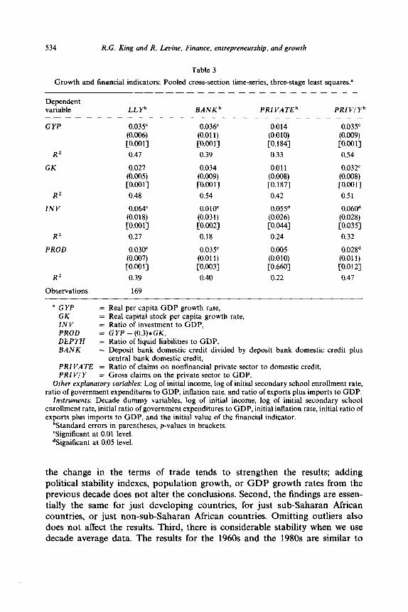
Table 3 summarizes the three-stage least squares (3SLS) results. The predict- able components of financial depth, the relative importance of banks as opposed to central banks, and the ratio of private credit to GDP are positively and significantly related to each growth indicator. The predictable component of financial development tends to be very strongly associated with growth and the sources of growth.
The results on the predictable components of financial development are fairly stable across a wide range of econometric specifications, including changes in the set of other explanatory variables, in the subsamples of countries, and in the subintervals of the full sample period. First, inclusion of continent dummies or
“The results also hold using pooled cross-section, time-series data with variables averaged over each decade, using various subsets of countries, or when including continent dummy variables, and with White’s heteroskedastic consistent standard errors. Working in the style of Levine and Renelt (1992), King and Levine (1993a) alter the conditioning information set by using various combina- tions of variables such as population growth, changes in the terms of trade, the number of revolutions and coups, the number of assassinations, the level of civil liberties, the standard deviation of inflation, domestic credit growth, the standard deviation of domestic credit growth, etc.
‘*To test for country effects (as opposed to continent effects), we subtracted the 1960-1989 mean of each variable from its value in each decade, computed the 3SLS results, and did a Hausman-type test to determine whether the coefficients on the two sets of results are significantly different from one another. This amounts to including dummy variables for each country and testing whether the coefficients on the financial indicators change. We find that the coefficients are not significantly different, which implies that we are not missing crucial country-specific effects. However, numerous coefficients change noticeably, but the standard error in the means-removed regression is such that means-removed coefficients are frequently less than one standard error away from the values in table 3. Thus, there may be some important country-specific effects that we are missing. As Easterly et al. (1993) show, real per capita GDP growth varies much more across decades than the economic indicators used to explain growth. Put differently, it will be difficult for cross-country growth regressions to explain fully a country’s growth experience because much of growth seems rooted in country-specific characteristics that are difficult to capture using available data on many countries over long time periods. The first-stage results indicate that the best predictor of the average level of financial development is past financial development. This emphasizes the relative lack of time-series variability in the explanatory variables we are using to explain growth.
534 R.G. King and R. Levine, Finance, entrepreneurship, and growth
Table 3
Growth and financial indicators: Pooled cross-section time-series, three-stage least squares.”
Dependent variable LL Yb BANKb PRIVATEb PRIVjY’
GYP
R2
GK
RZ
INV
R2
PROD
R2
Observations
0.035 0.036’ 0.014 0.035” (0.006) (0.011) (0.010) (0.009) [0.001] [O.OOl] [0.184] [0.001]
0.47 0.39 0.33 0.54
0.027 0.034 0.011 0.032’ (0.005) (0.009) (0.008) (0.008) [0.001] [O.OOl] [0.187] [O.OOl]
0.48 0.54 0.42 0.51
0.064’ 0.010’ 0.055d 0.060d (0.018) (0.03 1) (0.026) (0.028) [O.OOl] [0.002] [0.044] [0.035]
0.27 0.18 0.24 0.32
0.030’ 0.035’ 0.005 0.02gd (0.007) (0.011) (0.010) (0.011) [O.OOl] [0.003] [0.660] co.01 21
0.39 0.40 0.22 0.47
169
= GYP = Real per capita GDP growth rate, GK = Real capital stock per capita growth rate, INV = Ratio of investment to GDP, PROD = GYP - (0.3)*GK, DEPTH = Ratio of liquid liabilities to GDP, BANK = Deposit bank domestic credit divided by deposit bank domestic credit plus
central bank domestic credit, PRIVATE = Ratio of claims on nonfinancial private sector to domestic credit, PRIV/Y = Gross claims on the private sector to GDP.
Other explanatory variables: Log of initial income, log of initial secondary school enrollment rate, ratio of government expenditures to GDP, inflation rate, and ratio of exports plus imports to GDP.
Instruments: Decade dummy variables, log of initial income, log of initial secondary school enrollment rate, initial ratio of government expenditures to GDP, initial inflation rate, initial ratio of exports plus imports to GDP, and the initial value of the financial indicator.
%tandard errors in parentheses, p-values in brackets. ‘Significant at 0.01 level. %ignificant at 0.05 level.
the change in the terms of trade tends to strengthen the results; adding political stability indexes, population growth, or GDP growth rates from the previous decade does not alter the conclusions. Second, the findings are essen- tially the same for just developing countries, for just sub-Saharan African countries, or just non-sub-Saharan African countries. Omitting outliers also does not affect the results. Third, there is considerable stability when we use decade average data. The results for the 1960s and the 1980s are similar to
R.G. King and R. Levine. Finance. entrepreneurship. and growth 535
Table 4
Before and after financial sector reform.
Country BANK PRIVATE PRI Vi Y DEPTH CURRENCY REAL-RATE
Argentina 1974-76 1978-80
0.41 0.41 0.17 0.22 0.45 -44.70 0.81 0.59 0.16 0.21 0.26 - 14.13
Chile 1970-73 1977-81
- - 0.45 0.64
0.08 0.18 0.31 <o 0.28 0.17 0.19 8.80
Indonesia 1978-82 1984-89
0.53 0.40 0.09 0.15 0.38 -3.61 0.63 0.5 1 0.18 0.19 0.22 8.97
Korea 1978-80 1983-85
0.75 0.70 0.29 0.30 0.13 - 0.94 0.80 0.74 0.43 0.36 0.07 6.58
Philippines 1975-79 1981-84
0.77 0.72 0.22 0.22 0.13 - 2.09 0.72 0.65 0.29 0.26 0.12 - 3.03”
“If 1984 value of - 19.40 is omitted, the average annual real deposit interest rate over the 1981-83 period is 2.33.
results in table 3; for the 1970s only LLY and PRIVIY enter with significant coefficients in the 3SLS growth results.
3.2. Case studies
The cross-country regressions use financial development indicators, not measures of executable policies. In this subsection, we show that financial sector reforms in Argentina, Chile, Indonesia, Korea, and the Philippines were asso- ciated with increases in our financial development indicators [using the careful financial sector analyses in Bisat, Johnston, and Sundararajan (1992)]. While these reform episodes differ in terms of design and speed, there are basic similarities. Prior to reform, the government typically exerted a heavy hand in directing credit, setting interest rates, regulating the activities of existing finan- cial institutions, and restricting the emergence of new financial institutions. Reform involved the liberalization and relaxation of these controls and restrictions.
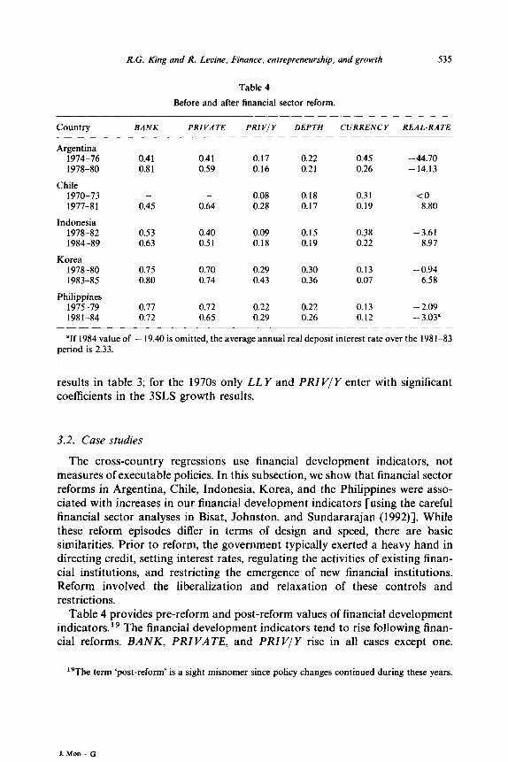
Table 4 provides pre-reform and post-reform values of financial development indicators.lg The financial development indicators tend to rise following finan- cial reforms. BANK, PRIVATE, and PRI V/Y rise in all cases except one.
“The term ‘post-reform’ is a sight misnomer since policy changes continued during these years.
1. Mm- 0
536 R.G. King and R. Levine. Finance, entrepreneurship. and growth
Financial depth, DEPTH, rises in Indonesia, Korea, and the Philippines and remains fairly stable in Argentina and Chile. Furthermore, the ratio of currency held outside of banks to bank deposits, CURRENCY, falls during every finan- cial reform program. Since drops in CURRENCY often indicate an increase in the level of financial intermediation, this additional indicator further suggests that financial reforms increase the public’s use of the formal financial sector. Also, during every reform episode except one, the real interest rate (REAL- RATE) rises: since liberalization typically involves the removal of interest rate ceilings, an increase in real interest rates may be used to measure the realization of advertised reforms. Thus, all of these indicators suggest that changes in financial sector policies are predictably associated with changes in aggregate measures of financial development.
However, three of the countries suffered financial crises after the financial reforms. Between March 1980 and March 1981, Argentine authorities liquidated financial institutions holding about 20 percent of total deposits. In Chile, by 1983, almost 20 per cent of commercial bank and finance company loans were in default. In the mid-1980s, the Philippine authorities had to move 30 percent of the banking system’s assets, which were nonperforming, to a government agency. Behind each crisis lies an unhealthy mix of financial liberalization combined with explicit or implicit official deposit guarantees and insufficient supervision. For example, in Argentina the weakest institutions offered the highest deposit interest rates, while on-site inspections by the Central Bank fell from 23 percent of banks before the reforms to 10 percent in 1981. Thus, while our financial indicators are positively associated with these particular financial reforms, it is also clear that the broad indicators do not indicate whether the underlying financial reforms are sustainable.
Furthermore, the available financial indicators may miss important develop- ments. For example, in Korea, nonbank financial intermediaries flourished during the mid-1980 financial liberalization. Nonbank credit grew from 18 percent of GDP in 1980 to 38 percent of GDP in 1988, while bank credit remained a constant share of GDP during this period. Thus, within our broad cross-section study, we are unable to include financial institutions other than banks: the case studies suggest that this may be a quantitatively important omission for some countries.
3.3. Firm-level studies of financial reform and credit allocation
Our theoretical model predicts that financial reforms should alter the flow of credit: more efficient firms should get a larger fraction of credit, and less efficient firms should get a smaller fraction of credit. A recent World Bank research project, discussed in Caprio (1994), sheds light on this mechanism. In particular, individual studies by Jaramillo, Schiantarelli, and Weiss (1993), Harris,
R.G. King and R. Levine, Finance, entrepreneurship, and growth 537
Schiantarelli, and Siregar (1992), and Siregar (1992) use firm-level panel data to examine the effects of financial sector reform in Ecuador and Indonesia on the allocation of credit.
To study the efficiency with which Ecuador and Indonesia allocate credit, these authors estimate a production function on firm-level data and then compute the distance that each firm lies from a production possibility frontier (defined by the most efficient firms). Firms closer to the frontier have higher ‘technical efficiency’.20 Based on a panel of several hundred Ecuadorian firms, ‘ . . . ceteris paribus, there has been an increase in the flow of credit accruing to technically more efficient firms, after liberalization, controlling for other firms’ characteristics’ [Caprio et al. (1994, ch. 5)]. The authors provide considerable evidence that the results are robust to different production function specifica- tions and estimation procedures. Furthermore, data on about two hundred Indonesian firms shows that credit flowed to more efficient firms following financial liberalization. Thus, financial liberalization was associated with a re- direction of the flow of credit to more efficient firms. This coincides with predictions of our model that financial intermediaries ‘add value’ by improving the selection and funding of entrepreneurs.
3.4. Structural adjustment and financial development
The model implies that the impact of nonfinancial, growth-promoting policy reforms will be greater if a country has a higher level of financial development, since it then may more effectively respond to changing incentives. The model also predicts that when financial liberalization accompanies nonfinancial policy reforms, the effect on growth will be greater than if financial reforms are not also undertaken. In practice, the effects of financial and nonfinancial policy reforms on growth will depend on many factors, including precisely which policies change, the order and speed of these changes, and the condition of the economy as a country initiates policy alterations. Instead of formally evaluating the interaction of the effects of various policy reforms on growth, we present suggestive evidence regarding the interplay between financial development, general policy reforms, and economic growth. Our hope is that this scrap of evidence will stimulate more detailed studies on this important topic.
In particular, we study whether the success of countries that engaged in intensive structural adjustment during the late 1980s depended on (a) the initial level of financial development and (b) financial liberalization during the reform episode. We define success in terms of the growth rate of per capita GDP. We define intensive structural adjustment in terms of the World Bank’s Third Report on Adjustment Lending. The Report classifies 27 nations as ‘intensive
“‘See the individual papers for detailed discussion of the procedure.
538 R.G. King and R. Levine, Finance. entrepreneurship, and growth
j
Ok-
Low High
Initial Financial Depth: 1985
Fig. 2. initial financial development and structural adjustment.
adjustment lending’ (IAL) countries during the second half of the group is defined as countries which received at least two structural
1980s. This adjustment _.
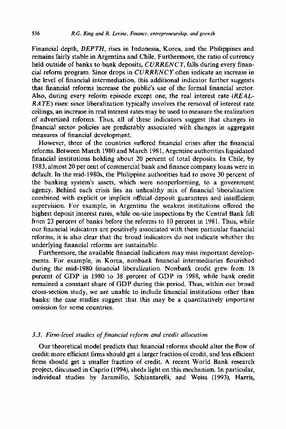
loans or three adjustment loans of any type (either structural or sectoral) between 1986 and 1990. These adjustment operations focused on trade liberal- ization, agricultural policy reforms, fiscal policy changes, on the removal of restrictive regulatory practices, and on public enterprise reform. Sometimes structural adjustment lending contained conditions on financial sector policy reforms. The Report shows that IAL countries grew faster in the later 1980s than other countries (those which did not receive any adjustment lending or countries which received only limited adjustment lending). Furthermore, the Report shows that IAL countries tended to implement policy reforms: public sector deficits fell, trade restrictions eased, black market premia fell, internal relative prices moved toward world levels, and IAL countries divested public companies2 1
“The Report also notes that adjustment takes years, and there may be significant recessions during the adjustment. The poor seem to benefit the most in the longer run from structural adjustment, but may suffer as the economy adjusts.
R.G. King and R. Levine. Finance, entrepreneurship, and growth 539
Financial Depth Growth: 1985 - 1990
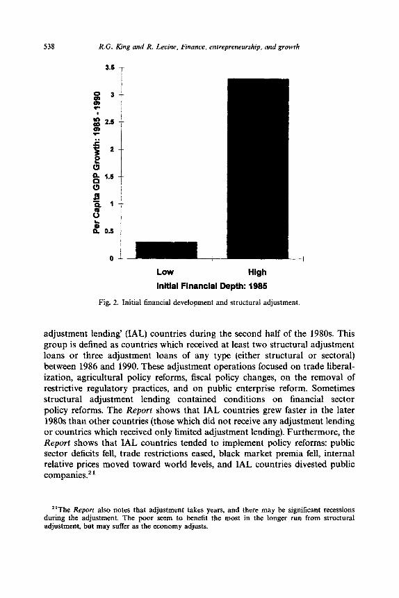
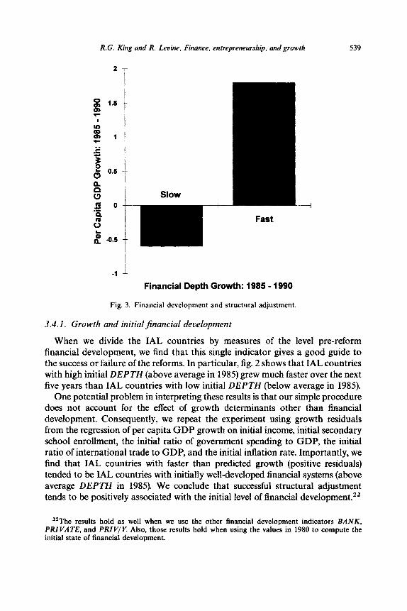
Fig. 3. Financial development and structural adjustment.
3.4.1. Growth and initial financial development
When we divide the IAL countries by measures of the level pre-reform financial development, we find that this single indicator gives a good guide to the success or failure of the reforms. In particular, fig. 2 shows that IAL countries with high initial DEPTH (above average in 1985) grew much faster over the next five years than IAL countries with low initial DEPTH (below average in 1985).
One potential problem in interpreting these results is that our simple procedure does not account for the effect of growth determinants other than financial development. Consequently, we repeat the experiment using growth residuals from the regression of per capita GDP growth on initial income, initial secondary school enrollment, the initial ratio of government spending to GDP, the initial ratio of international trade to GDP, and the initial inflation rate. Importantly, we find that IAL countries with faster than predicted growth (positive residuals) tended to be IAL countries with initially well-developed financial systems (above average DEPTH in 1985). We conclude that successful structural adjustment tends to be positively associated with the initial level of financial development.22
22The results hold as well when we use the other financial development indicators BANK, PRIVATE, and PRIV/Y. Also, those resufts hold when using the values in 1980 to compute the initial state of financial development.
540 R.G. King and R. Levine, Finance, entrepreneurship, and growth
3.4.2. Economic growth and financial sector growth
Fig. 3 shows that IAL countries with above-average financial development over the 1985-90 period - countries where DEPTH grew faster than average - grew much faster than IAL countries with below-average DEPTH growth. After controlling for other growth determinants, we find that IAL countries with faster than predicted growth tended to be IAL countries with financial systems that grew relatively rapidly. Successful structural adjustment tends to be posit- ively associated with an increased pace of financial development.
4. Conclusion
This paper articulates a new mechanism by which financial systems influence long-run economic growth. In our model, financial systems affect the entrepre- neurial activities that lead to productivity improvements in four ways. First, financial systems evaluate prospective entrepreneurs and choose the most prom- ising projects. Second, financial systems mobilize resources to finance promising projects. Third, financial systems allow investors to diversify the risk associated with uncertain innovative activities. Fourth, financial systems reveal the poten- tial rewards to engaging in innovation, relative to continuing to make existing products with existing techniques. Thus, a more-developed financial system fosters productivity improvement by choosing higher quality entrepreneurs and projects, by more effectively mobilizing external financing for these entrepre- neurs, by providing superior vehicles for diversifying the risk of innovative activities, and by revealing more accurately the potentially large profits asso- ciated with the uncertain business of innovation. In these ways, better financial systems stimulate economic growth by accelerating the rate of productivity enhancement.
There is much empirical support for this view. We reviewed a range of evidence concerning the links between financial sector development and growth, including cross-country regressions and case studies of the microeconomic and macroeconomic effects of financial sector and other policy reforms. We find support for the core idea advanced in our model: better financial systems stimulate faster productivity growth and growth in per capita output by funneling society’s resources to promising productivity-enhancing endeavors. Our findings suggest that government policies toward financial systems may have an important causal effect on long-run growth.
References
Aghion, P. and P. Howitt, 1992, A model of growth through creative destruction, Econometrica LX, 323-351.
R.G. King and R. Levine, Finance, entrepreneurship. and growth 541
Bencivenga, V.R. and B.D. Smith, 1991, Financial intermediation and endogenous growth, Review of Economic Studies LVIII, 195209.
Bencivenga, V.R. and B.D. Smith, 1992, Deficits, inflation and the banking system in developing countries: The optimal degree of financial repression, Oxford Economic Papers 44, 676-790.
Benhabib, J. and M. Speigel, 1992, Growth accounting with physical and human capital, Working paper (New York University, New York, NY).
Bhattacharya, S., 1992, Financial intermediation and proprietary information, Manuscript, July. Bisat, A., R.B. Johnston, and V. Sundararajan, 1992, Issues in managing and sequencing financial
sector reforms: Lessons from experiences in five developing countries, Working paper no. 82 (International Monetary Fund, Monetary and Exchange Affairs Department, Washington, DC).
Boyd, J.H. and E.C. Prescott, 1986, Financial intermediary coalitions, Journal of Economic Theory xxxv111, 211-212.
Boyd, J.H. and B.D. Smith, 1992, Intermediation and the equilibrium allocation of investment: Implications for economic development, Journal of Monetary Economics XXX, 409432.
Caprio, G., Jr., I. Atiyas, J.A. Hanson, and Associates, 1994, Financial reform: Theory and practice (Cambridge University Press, New York, NY) forthcoming.
Charnley, C. and P. Honohan, 1990, Taxation of financial intermediation, Working paper no. 421 (World Bank, Washington, DC).
DeGregorio, J. and P.E. Giudotti, 1992, Financial development and economic growth, Working paper no. 101 (International Monetary Fund, Monetary and Exchange Affairs Department, Washington, DC).
Diamond, D., 1984, Financial intermediation and delegated monitoring, Review of Economic Studies LI, 393-414.
Easterly, W., M. Kremer, L. Pritchett, and L.H. Summers, 1993, Good policy or good luck? Country growth performance and temporary shocks, Journal of Monetaryt Economics, this issue.
Fisher, I., 1930, The theory of interest of interest (MacMillan, New York, NY). Fry, M.J., 1988, Money, interest, and banking in economic development (Johns Hopkins University
Press, Baltimore, MD). Gelb, A., 1989, Financial policies, growth, and efficiency, Working paper no. 202 (World Bank,
Washington, DC). Gertler, M. and A. Rose, 1991, Finance, growth, and public policy, Working paper no. 814 (World
Bank, Washington, DC). Giovannini, A. and M. de Melo, 1993, Government revenue from financial repression, American
Economic Review VXXXIII, 953-963. Goldsmith, R.W., 1969, Financial structure and development (Yale University Press, New Haven,
CT). Greenwood, J. and B. Jovanovic, 1990, Financial development, growth, and the distribution of
income, Journal of Political Economy XCVIII, 10761107. Greenwood, J. and B.D. Smith, 1993, Financial markets in development, and the development of
financial markets, Journal of Economic Dynamics and Control, forthcoming. Grossman, G. and E. Helpman, 1991, Quality ladders in the theory of economic growth, Review of
Economic Studies LVIII, 43-61. Gurley, J.G. and E.S. Shaw, 1955, Financial aspects of economic development, American Economic
Review XLV, 515-538. Harris, J.R., F. Schiantarelli, and M.G. Siregar, 1993, How financial liberalization in Indonesia
affected firms’ capital structure and investment decisions, Working paper no. 997 (World Bank, Washington, DC).
Jaramillo, F., F. Schiantarelli, and A. Weiss, 1992, The effect of financial liberalization on the allocation of credit: Panel data evidence for Ecuador, Working paper no. 1092 (World Bank, Washington, DC).
King, R.G. and R. Levine, 1992a, Financial indicators and growth in a cross-section of countries, Working paper no. 819 (World Bank, Washington, DC).
King, R.G. and R. Levine, 1992b, Financial intermediation and economic development, in: C. Mayer and X. Vives, eds., Financial intermediation in the construction of Europe (Centre for Economic Policy Research, London).
King, R.G. and R. Levine, 1993a, Finance and growth: Schumpeter might be right, Quarterly Journal of Economics CVIII, 717-738.
542 R.G. King and R. Levine. Finance, entrepreneurship. and growth
King, R.G. and R. Levine, 1993b, Finance, entrepreneurship, and growth: Theory and evidence, Working paper (World Bank, Washington, DC).
King, R.G. and R. Levine, 1993c, Capital fundamentalism, economic development, and economic growth, Paper presented at the Carnegie-Rochester Conference Series on Public Policy.
Knight, F., 1952, Economic organization (Harper and Row, New York, NY). Levine, R., 1991, Stock markets, growth, and tax policy, Journal of Finance XLVI, 14451465. Levine, R. and D. Renelt, 1992, A sensitivity analysis of cross-country growth regressions, American
Economic Review LXXXII, 942-963. Lucas, R.E., Jr., 1988, On the mechanics of economic development, Journal of Monetary Economics
XXII, 3-42. McKinnon, RI., 1973, Money and capital in economic development (Brookings Institution,
Washington, DC). Pagano, M., 1993, Financial markets and growth: An overview, European Economic Review 37,
613-622. Rebelo, S., 1991, Long-run policy analysis and long-run growth, Journal of Political Economy IC,
500-521. Robinson, J., 1952, The generalization of the general theory, in: The rate of interest and other essays
(Macmillan, London). Romer, Paul M., 1990, Endogenous technological change, Journal of Political Economy XCVIII,
S71-SlO2. Roubini, N. and X. Sala-i-Martin, 1992, Financial repression and economic growth, Journal of
Development Economics XXXIX, S-50. Saint-Paul, G., 1992 Technological choice, financial markets and economic growth, European
Economic Review 37, 763-781. Schumpeter, Joseph A., 1912, Theorie der wirtschaftlichen Entwicklung (Dunker and Humboldt,
Leipzig); translated by Redvers Opie, 1934, The theory of economic development (Harvard University Press, Cambridge, MA).
Shleifer, A., 1986, Implementation cycles, Journal of Political Economy XCIV, 1163-l 190. Shaw, E.S., 1973, Financial deepening in economic development (Oxford University Press, New
York, NY). Siregar, M., 1992, Financial liberalization, investment and debt allocation, Unpublished Ph.D.
dissertation (Boston University, Boston, MA). Stern, N., 1989, The economics of development: A survey, The Economic Journal 100, 597-685. Solow, R.M., 1956, A contribution to the theory of economic growth, Quarterly Journal of
Economics LXX, 65-94. Solow, R.M., 1957, Technological change and the aggregate production function, Review of
Economics and Statistics XXXIX, 312-320. World Bank, 1989, World Bank development report (World Bank, Washington, DC). World Bank, 1992, The third report on adjustment lending: Private and public resources for growth
(World Bank, Washington, DC).