Embed Size (px)
Citation preview
BRINKER INTERNATIONAL
Financial Analysis Draft 3
Josh Moore, Brad Bolte, James Hall, Tanner Swaringen, Tim Meyer
4/1/2014
Page | 1
Table of Contents
Liquidity Ratios ...................................................................................................................................................... 3
Introduction ....................................................................................................................................................... 3
Current Ratio ..................................................................................................................................................... 3
Quick Ratio ......................................................................................................................................................... 4
Inventory Turnover ........................................................................................................................................ 5
Inventory Days ................................................................................................................................................. 7
Accounts Receivable Turnover .................................................................................................................. 8
Accounts Receivable Days ........................................................................................................................... 9
Cash to Cash Cycle ...................................................................................................................................... 10
Working Capital Turnover ......................................................................................................................... 11
Conclusion ........................................................................................................................................................ 12
Profitability Ratios ............................................................................................................................................. 12
Introduction .................................................................................................................................................... 12
Sales Growth ................................................................................................................................................... 12
Gross Profit Margin ...................................................................................................................................... 13
Operating Profit Margin ............................................................................................................................. 14
Net Profit Margin ........................................................................................................................................... 16
Asset Turnover............................................................................................................................................... 17
Return on Assets (“ROA”) ........................................................................................................................ 18
Return on Equity (“ROE”) ......................................................................................................................... 19
Conclusion ........................................................................................................................................................ 20
Capital Structure Ratios .................................................................................................................................. 20
Introduction .................................................................................................................................................... 20
Debt to Equity ................................................................................................................................................ 21
Times Interest Earned ................................................................................................................................ 22
Altman’s Z-Score ........................................................................................................................................... 23
Conclusion .................................................................................................................................................... 25
Growth Rates....................................................................................................................................................... 25
Introduction .................................................................................................................................................... 25
Internal Growth Rate .................................................................................................................................. 25
Sustainable Growth Rate .......................................................................................................................... 26
Page | 2
Industry-Specific Ratios ................................................................................................................................. 27
Introduction .................................................................................................................................................... 27
Company-Owned Locations ..................................................................................................................... 28
Financial Analysis Conclusion ...................................................................................................................... 29
Financial Forecasting ....................................................................................................................................... 29
Income Statement ....................................................................................................................................... 30
.............................................................................................................................................................................. 32
.............................................................................................................................................................................. 33
Dividends Forecasting ................................................................................................................................ 34
Balance Sheet................................................................................................................................................. 34
Statement of Cash Flows .......................................................................................................................... 40
.............................................................................................................................................................................. 41
Restated Financial Statements ............................................................................................................... 42
Cost of Capital Estimation ............................................................................................................................. 42
Cost of Debt .................................................................................................................................................... 42
Cost of Equity ................................................................................................................................................. 44
Backdoor Cost of Equity ............................................................................................................................ 47
Weighted Average Cost of Capital (WACC) ...................................................................................... 48
Appendix ................................................................................................................................................................ 53
Appendix (1) ........................................................................................................................................................ 53
Page | 3
Liquidity Ratios
Introduction Liquidity is the ability or quality of an asset that makes it easily convertible to
cash. In general, liquidity represents more safety to companies and investors alike
because it is easier for the holder of the asset to collect the cash value associated with
the asset. On a company balance sheet, marketable securities and accounts payable are
two examples of relatively liquid assets. In this analysis of liquidity ratios, we will looks
at the current and quick ratios, inventory turnover, inventory days, accounts receivable
turnover, accounts receivable days, cash to cash cycle, and working capital turnover.
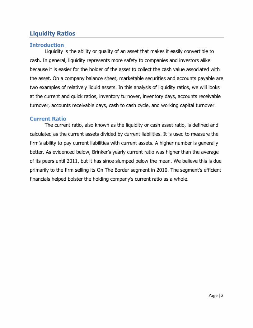
Current Ratio The current ratio, also known as the liquidity or cash asset ratio, is defined and
calculated as the current assets divided by current liabilities. It is used to measure the
firm’s ability to pay current liabilities with current assets. A higher number is generally
better. As evidenced below, Brinker’s yearly current ratio was higher than the average
of its peers until 2011, but it has since slumped below the mean. We believe this is due
primarily to the firm selling its On The Border segment in 2010. The segment’s efficient
financials helped bolster the holding company’s current ratio as a whole.
Page | 4
Current Ratio 2009 2010 2011 2012 2013 Average
Brinker 0.90 1.11 0.55 0.48 0.51 0.71 Brinker Restated 1.26 1.18 1.24 0.55 0.50 0.95 Dine Equity 1.31 1.32 1.07 1.10 1.17 1.19 Darden 0.51 0.54 0.52 0.43 0.54 0.51 Buffalo Wild Wings 1.48 1.70 1.22 0.89 1.10 1.28
Industry 1.09 1.17 0.92 0.69 0.76 0.93
Figure 1.
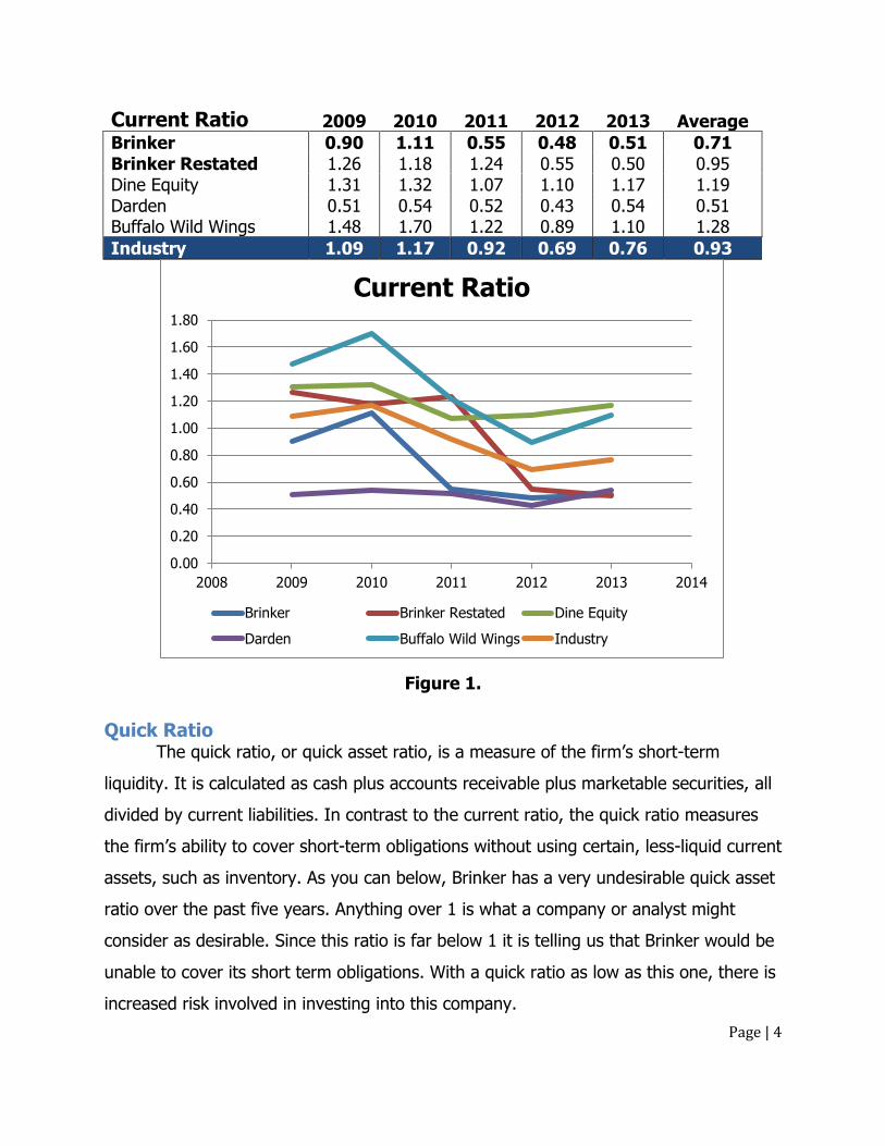
Quick Ratio The quick ratio, or quick asset ratio, is a measure of the firm’s short-term
liquidity. It is calculated as cash plus accounts receivable plus marketable securities, all
divided by current liabilities. In contrast to the current ratio, the quick ratio measures
the firm’s ability to cover short-term obligations without using certain, less-liquid current
assets, such as inventory. As you can below, Brinker has a very undesirable quick asset
ratio over the past five years. Anything over 1 is what a company or analyst might
consider as desirable. Since this ratio is far below 1 it is telling us that Brinker would be
unable to cover its short term obligations. With a quick ratio as low as this one, there is
increased risk involved in investing into this company.
0.00
0.20
0.40
0.60
0.80
1.00
1.20
1.40
1.60
1.80
2008 2009 2010 2011 2012 2013 2014
Current Ratio
Brinker Brinker Restated Dine Equity
Darden Buffalo Wild Wings Industry
Page | 5
Quick Ratio 2009 2010 2011 2012 2013 Average
Brinker 0.35 0.87 0.31 0.27 0.25 0.41 Brinker Restated 0.12 0.10 0.11 0.11 0.10 0.11 Dine Equity 0.72 0.76 0.68 0.72 0.88 0.75 Darden 0.06 0.24 0.11 0.08 0.12 0.12 Buffalo Wild Wings 0.83 0.93 0.64 0.36 0.52 0.66
Industry 0.42 0.58 0.37 0.31 0.37 0.41
Figure 2.
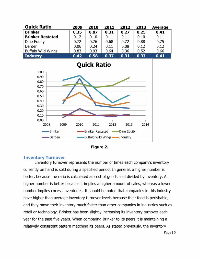
Inventory Turnover Inventory turnover represents the number of times each company’s inventory
currently on hand is sold during a specified period. In general, a higher number is
better, because the ratio is calculated as cost of goods sold divided by inventory. A
higher number is better because it implies a higher amount of sales, whereas a lower
number implies excess inventories. It should be noted that companies in this industry
have higher than average inventory turnover levels because their food is perishable,
and they move their inventory much faster than other companies in industries such as
retail or technology. Brinker has been slightly increasing its inventory turnover each
year for the past five years. When comparing Brinker to its peers it is maintaining a
relatively consistent pattern matching its peers. As stated previously, the inventory
0.00
0.10
0.20
0.30
0.40
0.50
0.60
0.70
0.80
0.90
1.00
2008 2009 2010 2011 2012 2013 2014
Quick Ratio
Brinker Brinker Restated Dine Equity
Darden Buffalo Wild Wings Industry
Page | 6
turnover in this industry is much higher than other industries due to the perishable
inventory. In this industry it is common to see this ratio exceeding 100, which Brinker
and its peers have done so over the past five years. In the last two years, Dine Equity
has shrunk its inventory to zero, while its percent of franchised restaurants has risen to
one hundred. That is why there are no inventory turnover statistics for Dine Equity over
the past two years.
Inventory Turnover 2009 2010 2011 2012 2013 Average
Brinker 98.63 106.90 108.87 111.23 115.56 108.24 Brinker Restated 106.98 106.92 108.87 111.23 115.56 109.91 Dine Equity 115.56 123.98 89.37 109.64 Darden 29.22 32.22 24.99 19.79 23.96 26.04 Buffalo Wild Wings 147.89 147.49 124.30 133.06 133.45 137.24
Industry 99.65 103.50 91.28 93.83 97.13 98.21
Figure 3.
0.00
20.00
40.00
60.00
80.00
100.00
120.00
140.00
160.00
2008 2009 2010 2011 2012 2013 2014
Inventory Turnover
Brinker Brinker Restated Dine Equity
Darden Buffalo Wild Wings Industry
Page | 7
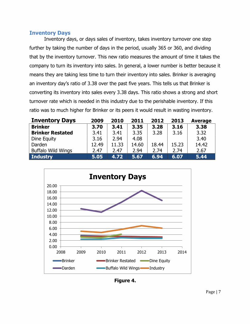
Inventory Days Inventory days, or days sales of inventory, takes inventory turnover one step
further by taking the number of days in the period, usually 365 or 360, and dividing
that by the inventory turnover. This new ratio measures the amount of time it takes the
company to turn its inventory into sales. In general, a lower number is better because it
means they are taking less time to turn their inventory into sales. Brinker is averaging
an inventory day’s ratio of 3.38 over the past five years. This tells us that Brinker is
converting its inventory into sales every 3.38 days. This ratio shows a strong and short
turnover rate which is needed in this industry due to the perishable inventory. If this
ratio was to much higher for Brinker or its peers it would result in wasting inventory.
Inventory Days 2009 2010 2011 2012 2013 Average
Brinker 3.70 3.41 3.35 3.28 3.16 3.38 Brinker Restated 3.41 3.41 3.35 3.28 3.16 3.32 Dine Equity 3.16 2.94 4.08 3.40 Darden 12.49 11.33 14.60 18.44 15.23 14.42 Buffalo Wild Wings 2.47 2.47 2.94 2.74 2.74 2.67
Industry 5.05 4.72 5.67 6.94 6.07 5.44
Figure 4.
0.00
2.00
4.00
6.00
8.00
10.00
12.00
14.00
16.00
18.00
20.00
2008 2009 2010 2011 2012 2013 2014
Inventory Days
Brinker Brinker Restated Dine Equity
Darden Buffalo Wild Wings Industry
Page | 8
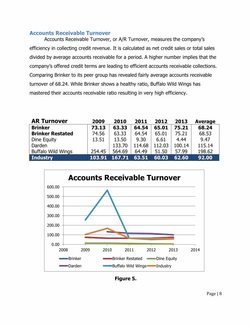
Accounts Receivable Turnover Accounts Receivable Turnover, or A/R Turnover, measures the company’s
efficiency in collecting credit revenue. It is calculated as net credit sales or total sales
divided by average accounts receivable for a period. A higher number implies that the
company’s offered credit terms are leading to efficient accounts receivable collections.
Comparing Brinker to its peer group has revealed fairly average accounts receivable
turnover of 68.24. While Brinker shows a healthy ratio, Buffalo Wild Wings has
mastered their accounts receivable ratio resulting in very high efficiency.
AR Turnover 2009 2010 2011 2012 2013 Average
Brinker 73.13 63.33 64.54 65.01 75.21 68.24 Brinker Restated 74.56 63.33 64.54 65.01 75.21 68.53 Dine Equity 13.51 13.50 9.30 6.61 4.44 9.47 Darden 133.70 114.68 112.03 100.14 115.14 Buffalo Wild Wings 254.45 564.69 64.49 51.50 57.99 198.62
Industry 103.91 167.71 63.51 60.03 62.60 92.00
Figure 5.
0.00
100.00
200.00
300.00
400.00
500.00
600.00
2008 2009 2010 2011 2012 2013 2014
Accounts Receivable Turnover
Brinker Brinker Restated Dine Equity
Darden Buffalo Wild Wings Industry
Page | 9
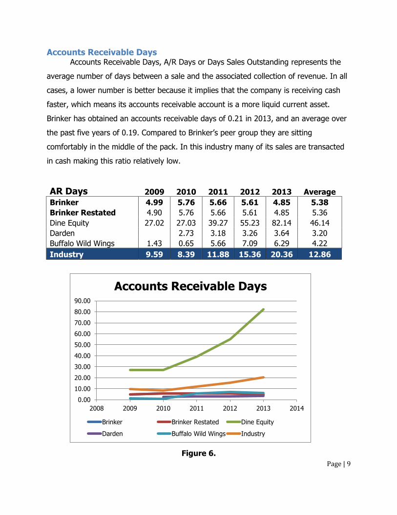
Accounts Receivable Days Accounts Receivable Days, A/R Days or Days Sales Outstanding represents the
average number of days between a sale and the associated collection of revenue. In all
cases, a lower number is better because it implies that the company is receiving cash
faster, which means its accounts receivable account is a more liquid current asset.
Brinker has obtained an accounts receivable days of 0.21 in 2013, and an average over
the past five years of 0.19. Compared to Brinker’s peer group they are sitting
comfortably in the middle of the pack. In this industry many of its sales are transacted
in cash making this ratio relatively low.
AR Days 2009 2010 2011 2012 2013 Average
Brinker 4.99 5.76 5.66 5.61 4.85 5.38
Brinker Restated 4.90 5.76 5.66 5.61 4.85 5.36
Dine Equity 27.02 27.03 39.27 55.23 82.14 46.14
Darden 2.73 3.18 3.26 3.64 3.20
Buffalo Wild Wings 1.43 0.65 5.66 7.09 6.29 4.22
Industry 9.59 8.39 11.88 15.36 20.36 12.86
Figure 6.
0.00
10.00
20.00
30.00
40.00
50.00
60.00
70.00
80.00
90.00
2008 2009 2010 2011 2012 2013 2014
Accounts Receivable Days
Brinker Brinker Restated Dine Equity
Darden Buffalo Wild Wings Industry
Page | 10
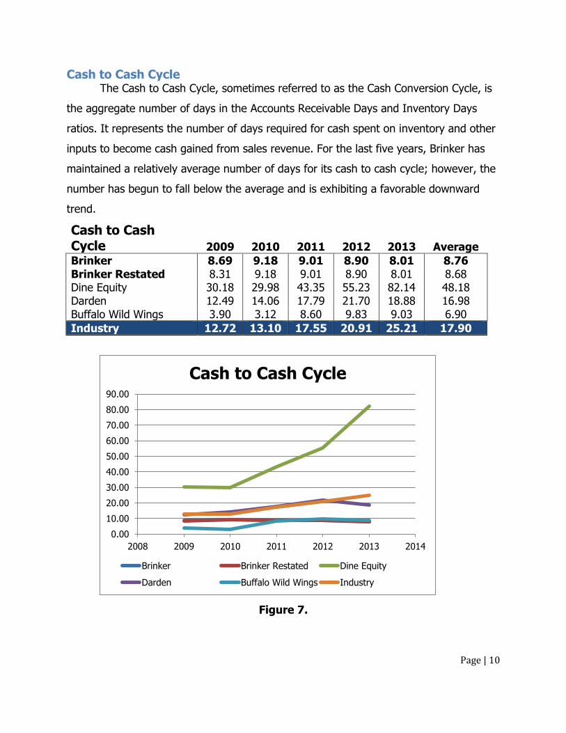
Cash to Cash Cycle The Cash to Cash Cycle, sometimes referred to as the Cash Conversion Cycle, is
the aggregate number of days in the Accounts Receivable Days and Inventory Days
ratios. It represents the number of days required for cash spent on inventory and other
inputs to become cash gained from sales revenue. For the last five years, Brinker has
maintained a relatively average number of days for its cash to cash cycle; however, the
number has begun to fall below the average and is exhibiting a favorable downward
trend.
Cash to Cash Cycle 2009 2010 2011 2012 2013 Average
Brinker 8.69 9.18 9.01 8.90 8.01 8.76 Brinker Restated 8.31 9.18 9.01 8.90 8.01 8.68 Dine Equity 30.18 29.98 43.35 55.23 82.14 48.18 Darden 12.49 14.06 17.79 21.70 18.88 16.98 Buffalo Wild Wings 3.90 3.12 8.60 9.83 9.03 6.90
Industry 12.72 13.10 17.55 20.91 25.21 17.90
Figure 7.
0.00
10.00
20.00
30.00
40.00
50.00
60.00
70.00
80.00
90.00
2008 2009 2010 2011 2012 2013 2014
Cash to Cash Cycle
Brinker Brinker Restated Dine Equity
Darden Buffalo Wild Wings Industry
Page | 11
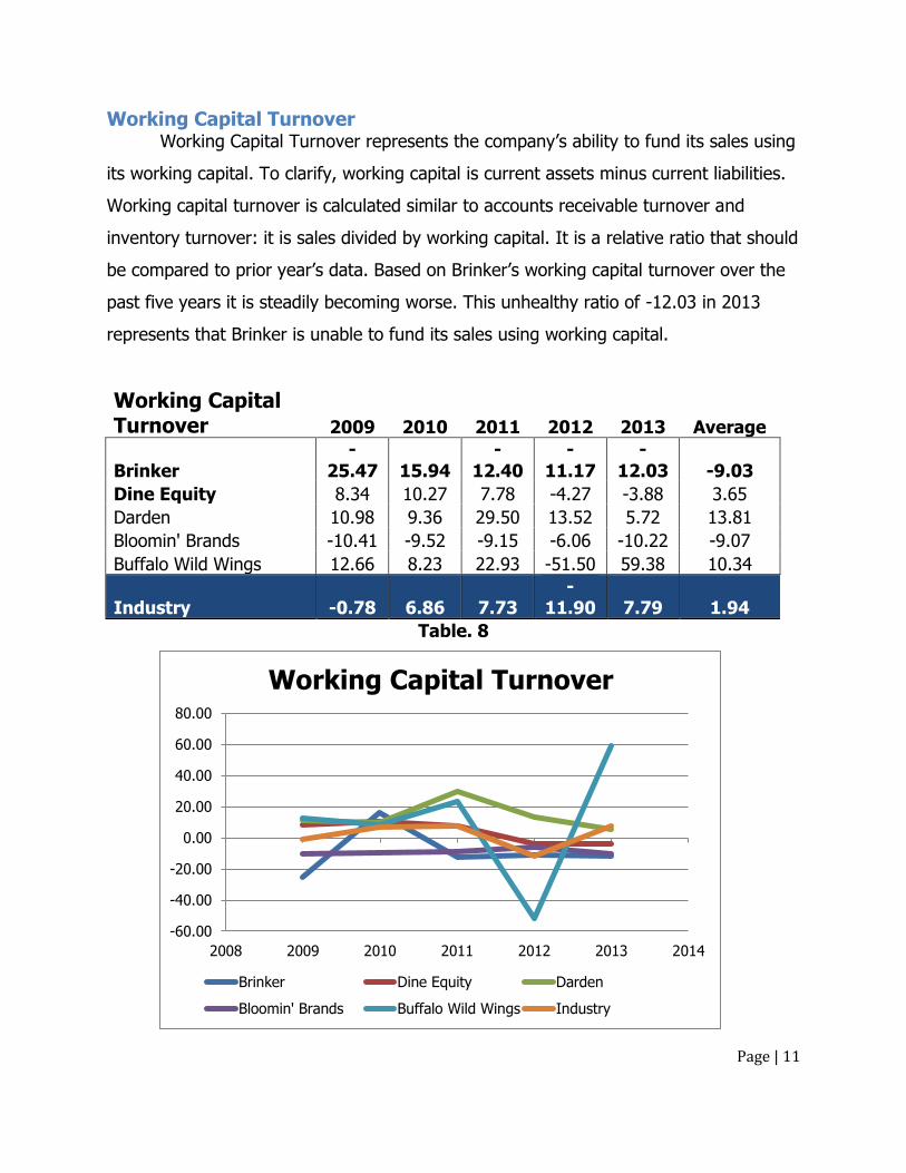
Working Capital Turnover Working Capital Turnover represents the company’s ability to fund its sales using
its working capital. To clarify, working capital is current assets minus current liabilities.
Working capital turnover is calculated similar to accounts receivable turnover and
inventory turnover: it is sales divided by working capital. It is a relative ratio that should
be compared to prior year’s data. Based on Brinker’s working capital turnover over the
past five years it is steadily becoming worse. This unhealthy ratio of -12.03 in 2013
represents that Brinker is unable to fund its sales using working capital.
Working Capital Turnover 2009 2010 2011 2012 2013 Average
Brinker -
25.47 15.94 -
12.40 -
11.17 -
12.03 -9.03
Dine Equity 8.34 10.27 7.78 -4.27 -3.88 3.65
Darden 10.98 9.36 29.50 13.52 5.72 13.81
Bloomin' Brands -10.41 -9.52 -9.15 -6.06 -10.22 -9.07
Buffalo Wild Wings 12.66 8.23 22.93 -51.50 59.38 10.34
Industry -0.78 6.86 7.73 -
11.90 7.79 1.94
Table. 8
-60.00
-40.00
-20.00
0.00
20.00
40.00
60.00
80.00
2008 2009 2010 2011 2012 2013 2014
Working Capital Turnover
Brinker Dine Equity Darden
Bloomin' Brands Buffalo Wild Wings Industry
Page | 12
Figure 8.
Conclusion After rigorous analysis of Brinker’s liquidity ratios many of their ratios are
undesirable, representing an increased amount of risk involved in investing in this
company. Given these low liquidity ratios, representing Brinker we can come to the
conclusion that the margin for safety if significantly lower than the industry average.
We will discuss Brinker’s likelihood of going bankrupt with the Altman’s Z-score later in
this ration analysis section.
Profitability Ratios
Introduction Profitability ratios assess the extent to which a company’s revenues exceed
various measures of their cost. As a rule of thumb the higher this ratio is compared to
its competitors the better shape the company is in. Profitability ratios are the most
commonly analyzed ratios when an investor is doing a financial analysis. These ratios by
themselves may not make sense at certain times. It is important to have a good overall
understanding of the industry from where these ratios are being taken in order to
complete the entire story that this analysis will provide.
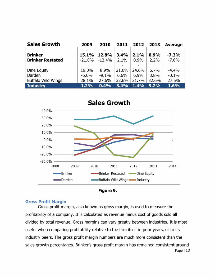
Sales Growth Sales Growth is the percentage change of sales from one year to the next. A
higher number is considered to be the most desirable figure for this ratio. While it does
not factor in the associated cost of revenue, it can be a useful statistic in measuring the
firms’ growth or accumulation of the market share compared to its peer. Brinker’s sales
decreased from 2009 to 2011, but have since displayed an upward trend. The sales
numbers are very volatile within this peer group, but Brinker’s numbers are generally
lower than the average.
Page | 13
Sales Growth 2009 2010 2011 2012 2013 Average
Brinker -
15.1% -
12.8% -
3.4% 2.1% 0.9% -7.3% Brinker Restated -21.0% -12.4% 2.1% 0.9% 2.2% -7.6%
Dine Equity 19.0% 8.9% -
21.0% -
24.6% 6.7% -4.4% Darden -5.0% -9.1% 6.6% 6.9% 3.8% -0.1% Buffalo Wild Wings 28.1% 27.6% 32.6% 21.7% 32.6% 27.5%
Industry 1.2% 0.4% 3.4% 1.4% 9.2% 1.6%
Figure 9.
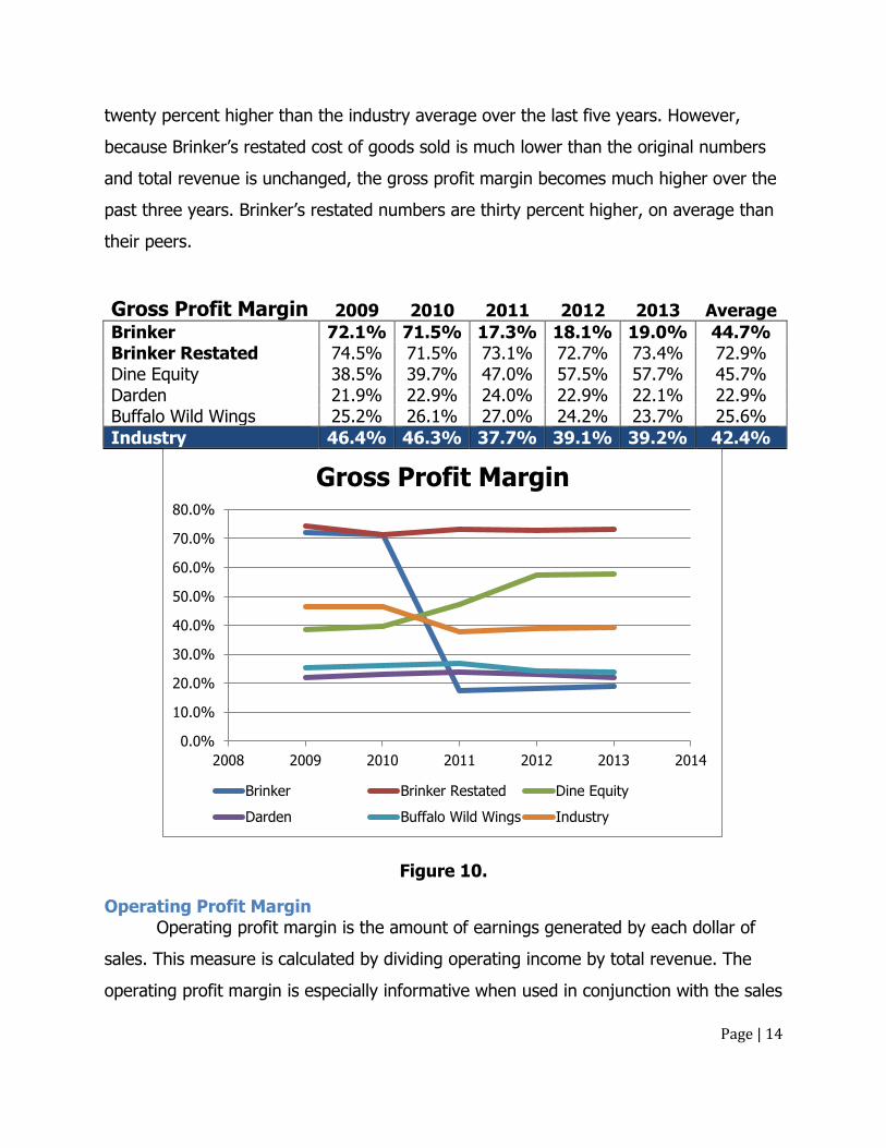
Gross Profit Margin Gross profit margin, also known as gross margin, is used to measure the
profitability of a company. It is calculated as revenue minus cost of goods sold all
divided by total revenue. Gross margins can vary greatly between industries. It is most
useful when comparing profitability relative to the firm itself in prior years, or to its
industry peers. The gross profit margin numbers are much more consistent than the
sales growth percentages. Brinker’s gross profit margin has remained consistent around
-30.0%
-20.0%
-10.0%
0.0%
10.0%
20.0%
30.0%
40.0%
2008 2009 2010 2011 2012 2013 2014
Sales Growth
Brinker Brinker Restated Dine Equity
Darden Buffalo Wild Wings Industry
Page | 14
twenty percent higher than the industry average over the last five years. However,
because Brinker’s restated cost of goods sold is much lower than the original numbers
and total revenue is unchanged, the gross profit margin becomes much higher over the
past three years. Brinker’s restated numbers are thirty percent higher, on average than
their peers.
Gross Profit Margin 2009 2010 2011 2012 2013 Average
Brinker 72.1% 71.5% 17.3% 18.1% 19.0% 44.7% Brinker Restated 74.5% 71.5% 73.1% 72.7% 73.4% 72.9% Dine Equity 38.5% 39.7% 47.0% 57.5% 57.7% 45.7% Darden 21.9% 22.9% 24.0% 22.9% 22.1% 22.9% Buffalo Wild Wings 25.2% 26.1% 27.0% 24.2% 23.7% 25.6%
Industry 46.4% 46.3% 37.7% 39.1% 39.2% 42.4%
Figure 10.
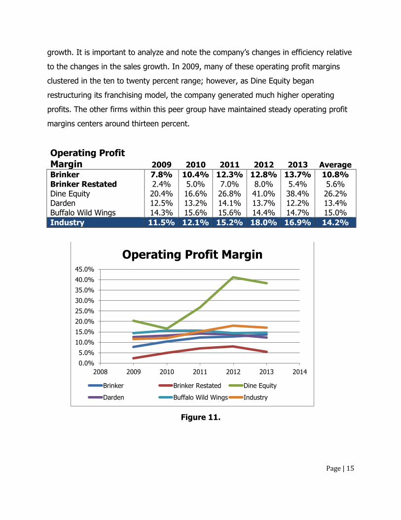
Operating Profit Margin Operating profit margin is the amount of earnings generated by each dollar of
sales. This measure is calculated by dividing operating income by total revenue. The
operating profit margin is especially informative when used in conjunction with the sales
0.0%
10.0%
20.0%
30.0%
40.0%
50.0%
60.0%
70.0%
80.0%
2008 2009 2010 2011 2012 2013 2014
Gross Profit Margin
Brinker Brinker Restated Dine Equity
Darden Buffalo Wild Wings Industry
Page | 15
growth. It is important to analyze and note the company’s changes in efficiency relative
to the changes in the sales growth. In 2009, many of these operating profit margins
clustered in the ten to twenty percent range; however, as Dine Equity began
restructuring its franchising model, the company generated much higher operating
profits. The other firms within this peer group have maintained steady operating profit
margins centers around thirteen percent.
Operating Profit Margin 2009 2010 2011 2012 2013 Average
Brinker 7.8% 10.4% 12.3% 12.8% 13.7% 10.8% Brinker Restated 2.4% 5.0% 7.0% 8.0% 5.4% 5.6% Dine Equity 20.4% 16.6% 26.8% 41.0% 38.4% 26.2% Darden 12.5% 13.2% 14.1% 13.7% 12.2% 13.4% Buffalo Wild Wings 14.3% 15.6% 15.6% 14.4% 14.7% 15.0%
Industry 11.5% 12.1% 15.2% 18.0% 16.9% 14.2%
Figure 11.
0.0%
5.0%
10.0%
15.0%
20.0%
25.0%
30.0%
35.0%
40.0%
45.0%
2008 2009 2010 2011 2012 2013 2014
Operating Profit Margin
Brinker Brinker Restated Dine Equity
Darden Buffalo Wild Wings Industry
Page | 16
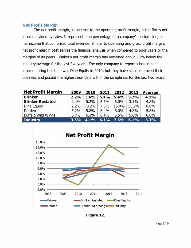
Net Profit Margin The net profit margin, in contrast to the operating profit margin, is the firm’s net
income divided by sales. It represents the percentage of a company’s bottom line, or
net income that comprises total revenue. Similar to operating and gross profit margin,
net profit margin best serves the financial analysis when compared to prior years or the
margins of its peers. Brinker’s net profit margin has remained about 1.2% below the
industry average for the last five years. The only company to report a loss in net
income during this time was Dine Equity in 2010, but they have since improved their
business and posted the highest numbers within the sample set for the last two years.
Net Profit Margin 2009 2010 2011 2012 2013 Average
Brinker 2.2% 3.6% 5.1% 5.4% 5.7% 4.1% Brinker Restated 2.4% 5.2% 5.5% 6.0% 3.1% 4.8% Dine Equity 2.2% -0.2% 7.0% 15.0% 11.2% 6.0% Darden 5.2% 5.8% 6.4% 6.0% 4.8% 5.8% Buffalo Wild Wings 5.7% 6.3% 6.4% 5.5% 5.6% 6.0%
Industry 3.5% 4.1% 6.1% 7.6% 6.1% 5.3%
Figure 12.
-2.0%
0.0%
2.0%
4.0%
6.0%
8.0%
10.0%
12.0%
14.0%
16.0%
2008 2009 2010 2011 2012 2013 2014
Net Profit Margin
Brinker Brinker Restated Dine Equity
Darden Buffalo Wild Wings Industry
Page | 17
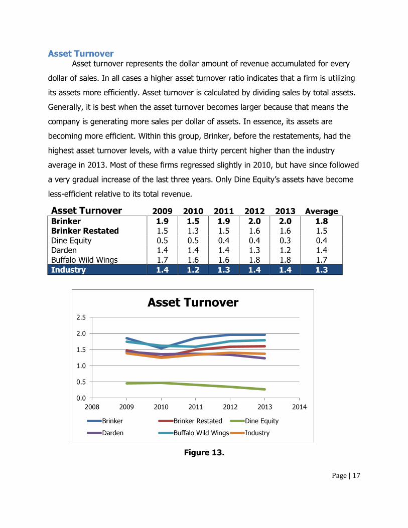
Asset Turnover Asset turnover represents the dollar amount of revenue accumulated for every
dollar of sales. In all cases a higher asset turnover ratio indicates that a firm is utilizing
its assets more efficiently. Asset turnover is calculated by dividing sales by total assets.
Generally, it is best when the asset turnover becomes larger because that means the
company is generating more sales per dollar of assets. In essence, its assets are
becoming more efficient. Within this group, Brinker, before the restatements, had the
highest asset turnover levels, with a value thirty percent higher than the industry
average in 2013. Most of these firms regressed slightly in 2010, but have since followed
a very gradual increase of the last three years. Only Dine Equity’s assets have become
less-efficient relative to its total revenue.
Asset Turnover 2009 2010 2011 2012 2013 Average
Brinker 1.9 1.5 1.9 2.0 2.0 1.8 Brinker Restated 1.5 1.3 1.5 1.6 1.6 1.5 Dine Equity 0.5 0.5 0.4 0.4 0.3 0.4 Darden 1.4 1.4 1.4 1.3 1.2 1.4 Buffalo Wild Wings 1.7 1.6 1.6 1.8 1.8 1.7
Industry 1.4 1.2 1.3 1.4 1.4 1.3
Figure 13.
0.0
0.5
1.0
1.5
2.0
2.5
2008 2009 2010 2011 2012 2013 2014
Asset Turnover
Brinker Brinker Restated Dine Equity
Darden Buffalo Wild Wings Industry
Page | 18
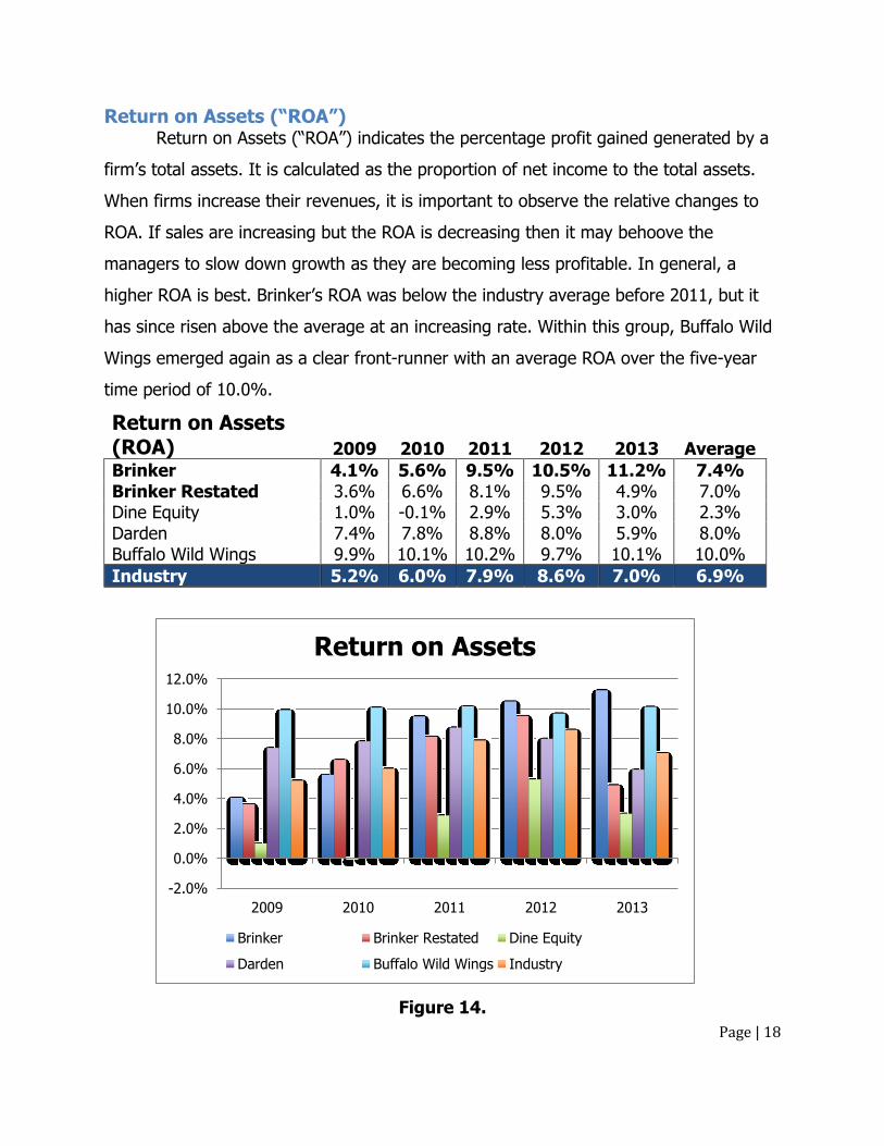
Return on Assets (“ROA”) Return on Assets (“ROA”) indicates the percentage profit gained generated by a
firm’s total assets. It is calculated as the proportion of net income to the total assets.
When firms increase their revenues, it is important to observe the relative changes to
ROA. If sales are increasing but the ROA is decreasing then it may behoove the
managers to slow down growth as they are becoming less profitable. In general, a
higher ROA is best. Brinker’s ROA was below the industry average before 2011, but it
has since risen above the average at an increasing rate. Within this group, Buffalo Wild
Wings emerged again as a clear front-runner with an average ROA over the five-year
time period of 10.0%.
Return on Assets (ROA) 2009 2010 2011 2012 2013 Average
Brinker 4.1% 5.6% 9.5% 10.5% 11.2% 7.4% Brinker Restated 3.6% 6.6% 8.1% 9.5% 4.9% 7.0% Dine Equity 1.0% -0.1% 2.9% 5.3% 3.0% 2.3% Darden 7.4% 7.8% 8.8% 8.0% 5.9% 8.0% Buffalo Wild Wings 9.9% 10.1% 10.2% 9.7% 10.1% 10.0%
Industry 5.2% 6.0% 7.9% 8.6% 7.0% 6.9%
Figure 14.
-2.0%
0.0%
2.0%
4.0%
6.0%
8.0%
10.0%
12.0%
2009 2010 2011 2012 2013
Return on Assets
Brinker Brinker Restated Dine Equity
Darden Buffalo Wild Wings Industry
Page | 19
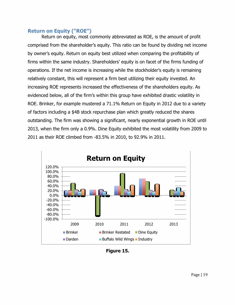
Return on Equity (“ROE”) Return on equity, most commonly abbreviated as ROE, is the amount of profit
comprised from the shareholder’s equity. This ratio can be found by dividing net income
by owner’s equity. Return on equity best utilized when comparing the profitability of
firms within the same industry. Shareholders’ equity is on facet of the firms funding of
operations. If the net income is increasing while the stockholder’s equity is remaining
relatively constant, this will represent a firm best utilizing their equity invested. An
increasing ROE represents increased the effectiveness of the shareholders equity. As
evidenced below, all of the firm’s within this group have exhibited drastic volatility in
ROE. Brinker, for example mustered a 71.1% Return on Equity in 2012 due to a variety
of factors including a $4B stock repurchase plan which greatly reduced the shares
outstanding. The firm was showing a significant, nearly exponential growth in ROE until
2013, when the firm only a 0.9%. Dine Equity exhibited the most volatility from 2009 to
2011 as their ROE climbed from -83.5% in 2010, to 92.9% in 2011.
Figure 15.
-100.0%
-80.0%
-60.0%
-40.0%
-20.0%
0.0%
20.0%
40.0%
60.0%
80.0%
100.0%
120.0%
2009 2010 2011 2012 2013
Return on Equity
Brinker Brinker Restated Dine Equity
Darden Buffalo Wild Wings Industry
Page | 20
Figure 16.
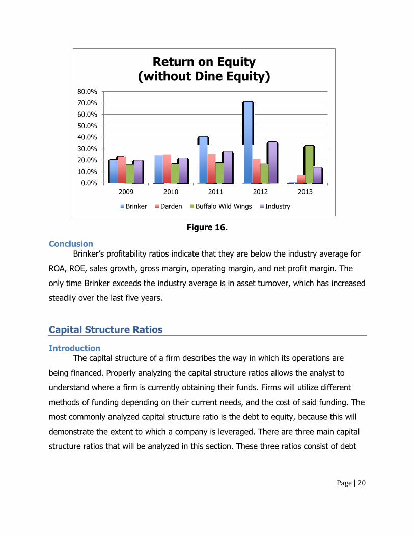
Conclusion Brinker’s profitability ratios indicate that they are below the industry average for
ROA, ROE, sales growth, gross margin, operating margin, and net profit margin. The
only time Brinker exceeds the industry average is in asset turnover, which has increased
steadily over the last five years.
Capital Structure Ratios
Introduction The capital structure of a firm describes the way in which its operations are
being financed. Properly analyzing the capital structure ratios allows the analyst to
understand where a firm is currently obtaining their funds. Firms will utilize different
methods of funding depending on their current needs, and the cost of said funding. The
most commonly analyzed capital structure ratio is the debt to equity, because this will
demonstrate the extent to which a company is leveraged. There are three main capital
structure ratios that will be analyzed in this section. These three ratios consist of debt
0.0%
10.0%
20.0%
30.0%
40.0%
50.0%
60.0%
70.0%
80.0%
2009 2010 2011 2012 2013
Return on Equity (without Dine Equity)
Brinker Darden Buffalo Wild Wings Industry
Page | 21
to equity, times interest earned, and the Altman’s Z-score, which will be discussed in
further detail below.
Debt to Equity The Debt to Equity Ratio is a capital structure ratio that measures the firm’s
debt, or total liabilities, in proportion to total shareholders equity. In order to confirm
the most universal truth of accounting, assets must always equal liabilities plus
shareholders’ equity. The Debt to Equity Ratio describes the amount of leverage or debt
that comprises that latter part of the equation. Analyst opinions vary regarding an ideal
number for this ratio. For instance, a higher number indicates that the firm has been
aggressive in financing its assets with debt, which has trade-offs. If the growth rate of
the company is less than the cost of debt, then creditors benefit. Relative to its peer
group Brinker is doing very well about not financing a majority of its assets with debt.
Brinker has been able to obtain a debt to equity ratio of 0.34 while its peer group
average is 0.66. It is also important to point out that Buffalo Wild Wings has been able
to finance all of its assets without seeking debt.
Debt to Equity 2009 2010 2011 2012 2013 Average
Brinker 0.37 0.33 0.36 0.30 0.36 0.34
Brinker Restated 0.37 0.32 0.34 0.29 0.34 0.33
Dine Equity 4.98 2.25 2.27 1.08 0.76 2.27
Darden 0.3 0.27 0.31 0.40 0.36 0.33
Buffalo Wild Wings 0.00 0.00 0.00 0.00 0.00 0.00
Industry 1.21 0.64 0.66 0.41 0.36 0.66
0.00
1.00
2.00
3.00
4.00
5.00
6.00
2008 2009 2010 2011 2012 2013 2014
Debt to Equity
Brinker Brinker Restated
Dine Equity Darden
Buffalo Wild Wings Industry
Page | 22
Figure 17.
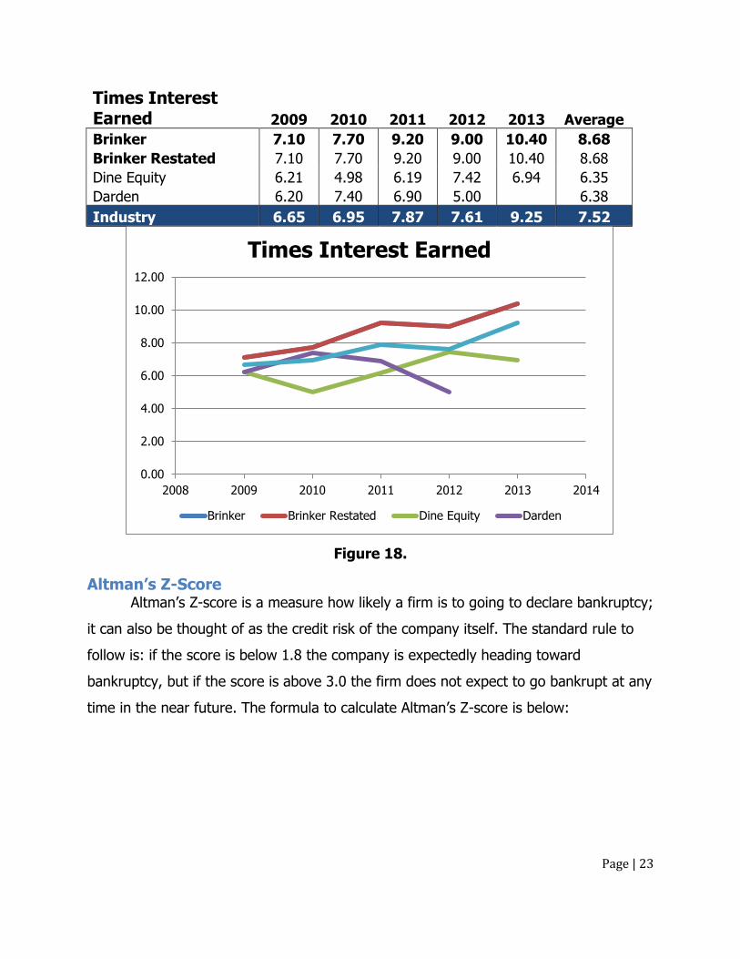
Times Interest Earned Times interest earned is useful when analyzing the proportion of interest that
comprises operating income. It is the number of times a company can pay its interest
expenses out of the earnings before interest and taxes account. Anything below one is
considered to be undesirable and risky to potential investors. This ratio is attained by
dividing earnings before interest and taxed by total interest payable. Over the past
three years, all of the firms in this group, except Darden, have exhibited a strong
upward trend in times interest earned. Their total revenues are beginning to cover a
larger amount of the interest owed on outstanding debt. Because Buffalo Wild Wings is
debt-free, it does not need to pay interest on any debt. Thus, the times interest earned
ratio is undefined.
Page | 23
Times Interest Earned 2009 2010 2011 2012 2013 Average
Brinker 7.10 7.70 9.20 9.00 10.40 8.68
Brinker Restated 7.10 7.70 9.20 9.00 10.40 8.68
Dine Equity 6.21 4.98 6.19 7.42 6.94 6.35
Darden 6.20 7.40 6.90 5.00 6.38
Industry 6.65 6.95 7.87 7.61 9.25 7.52
Figure 18.
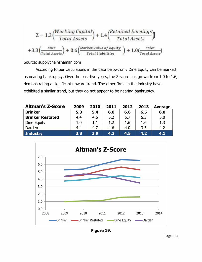
Altman’s Z-Score Altman’s Z-score is a measure how likely a firm is to going to declare bankruptcy;
it can also be thought of as the credit risk of the company itself. The standard rule to
follow is: if the score is below 1.8 the company is expectedly heading toward
bankruptcy, but if the score is above 3.0 the firm does not expect to go bankrupt at any
time in the near future. The formula to calculate Altman’s Z-score is below:
0.00
2.00
4.00
6.00
8.00
10.00
12.00
2008 2009 2010 2011 2012 2013 2014
Times Interest Earned
Brinker Brinker Restated Dine Equity Darden
Page | 24
Source: supplychainshaman.com
According to our calculations in the data below, only Dine Equity can be marked
as nearing bankruptcy. Over the past five years, the Z-score has grown from 1.0 to 1.6,
demonstrating a significant upward trend. The other firms in the industry have
exhibited a similar trend, but they do not appear to be nearing bankruptcy.
Altman's Z-Score 2009 2010 2011 2012 2013 Average
Brinker 5.3 5.4 6.0 6.6 6.5 6.0
Brinker Restated 4.4 4.6 5.2 5.7 5.3 5.0
Dine Equity 1.0 1.1 1.2 1.6 1.6 1.3
Darden 4.4 4.7 4.6 4.0 3.5 4.2
Industry 3.8 3.9 4.2 4.5 4.2 4.1
Figure 19.
0.0
1.0
2.0
3.0
4.0
5.0
6.0
7.0
2008 2009 2010 2011 2012 2013 2014
Altman's Z-Score
Brinker Brinker Restated Dine Equity Darden
Page | 25
Conclusion
As evidenced by the debt to equity ratio, the percentage of invested capital
allocated to debt is generally lower in this industry, with the exception of Dine Equity,
whom has seven times the amount of debt as they do equity, which may be negative
affects their bankruptcy risk in the Altman’s Z-score. For the most part, Brinker’s capital
structure numbers are on par with many of the statistics of the casual dining sector as a
whole, despite the volatility within this small peer group.
Growth Rates
Introduction In this section, there are two relevant growth rates to be analyzed: internal
growth rate and sustainable growth rate. The sustainable growth rate measures the
level of growth attainable while receiving no outside additional funding. The internal
growth rate is used to assess the ability to which a firm can grow by keeping its capital
structure constant.
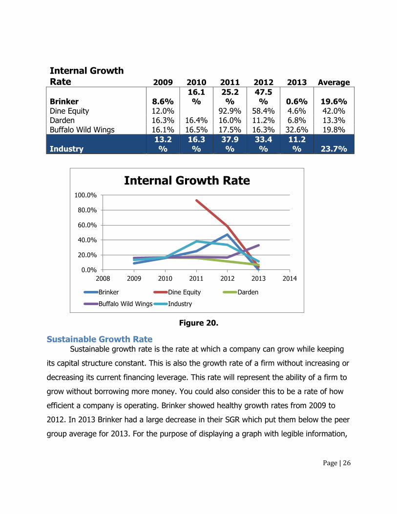
Internal Growth Rate Internal growth rate is the level of a firm’s growth rate without obtaining
financing from outside sources. This ratio is very important for smaller firms and startup
firms. If a firm is able to obtain a healthy internal growth rate is represents the ability of
a company to grow with only its available assets. After analyzing Brinker’s IGR over the
past five years, there has not been a noticeable trend associated with this information.
Brinker’s five year average is consistent with its peer group average, which shows it is
similar to the rest of its competitors.
Page | 26
Internal Growth Rate 2009 2010 2011 2012 2013 Average
Brinker 8.6% 16.1%
25.2%
47.5% 0.6% 19.6%
Dine Equity 12.0% 92.9% 58.4% 4.6% 42.0% Darden 16.3% 16.4% 16.0% 11.2% 6.8% 13.3% Buffalo Wild Wings 16.1% 16.5% 17.5% 16.3% 32.6% 19.8%
Industry 13.2%
16.3%
37.9%
33.4%
11.2% 23.7%
Figure 20.
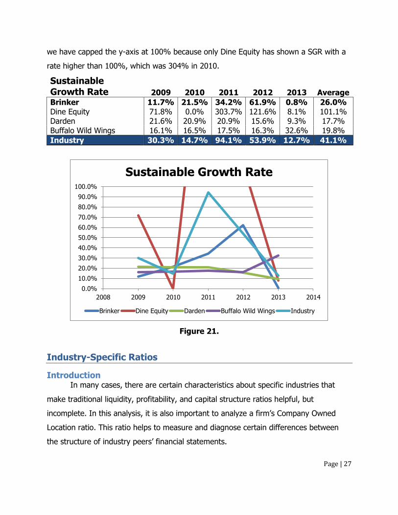
Sustainable Growth Rate Sustainable growth rate is the rate at which a company can grow while keeping
its capital structure constant. This is also the growth rate of a firm without increasing or
decreasing its current financing leverage. This rate will represent the ability of a firm to
grow without borrowing more money. You could also consider this to be a rate of how
efficient a company is operating. Brinker showed healthy growth rates from 2009 to
2012. In 2013 Brinker had a large decrease in their SGR which put them below the peer
group average for 2013. For the purpose of displaying a graph with legible information,
0.0%
20.0%
40.0%
60.0%
80.0%
100.0%
2008 2009 2010 2011 2012 2013 2014
Internal Growth Rate
Brinker Dine Equity Darden
Buffalo Wild Wings Industry
Page | 27
we have capped the y-axis at 100% because only Dine Equity has shown a SGR with a
rate higher than 100%, which was 304% in 2010.
Sustainable Growth Rate 2009 2010 2011 2012 2013 Average
Brinker 11.7% 21.5% 34.2% 61.9% 0.8% 26.0% Dine Equity 71.8% 0.0% 303.7% 121.6% 8.1% 101.1% Darden 21.6% 20.9% 20.9% 15.6% 9.3% 17.7% Buffalo Wild Wings 16.1% 16.5% 17.5% 16.3% 32.6% 19.8%
Industry 30.3% 14.7% 94.1% 53.9% 12.7% 41.1%
Figure 21.
Industry-Specific Ratios
Introduction In many cases, there are certain characteristics about specific industries that
make traditional liquidity, profitability, and capital structure ratios helpful, but
incomplete. In this analysis, it is also important to analyze a firm’s Company Owned
Location ratio. This ratio helps to measure and diagnose certain differences between
the structure of industry peers’ financial statements.
0.0%
10.0%
20.0%
30.0%
40.0%
50.0%
60.0%
70.0%
80.0%
90.0%
100.0%
2008 2009 2010 2011 2012 2013 2014
Sustainable Growth Rate
Brinker Dine Equity Darden Buffalo Wild Wings Industry
Page | 28
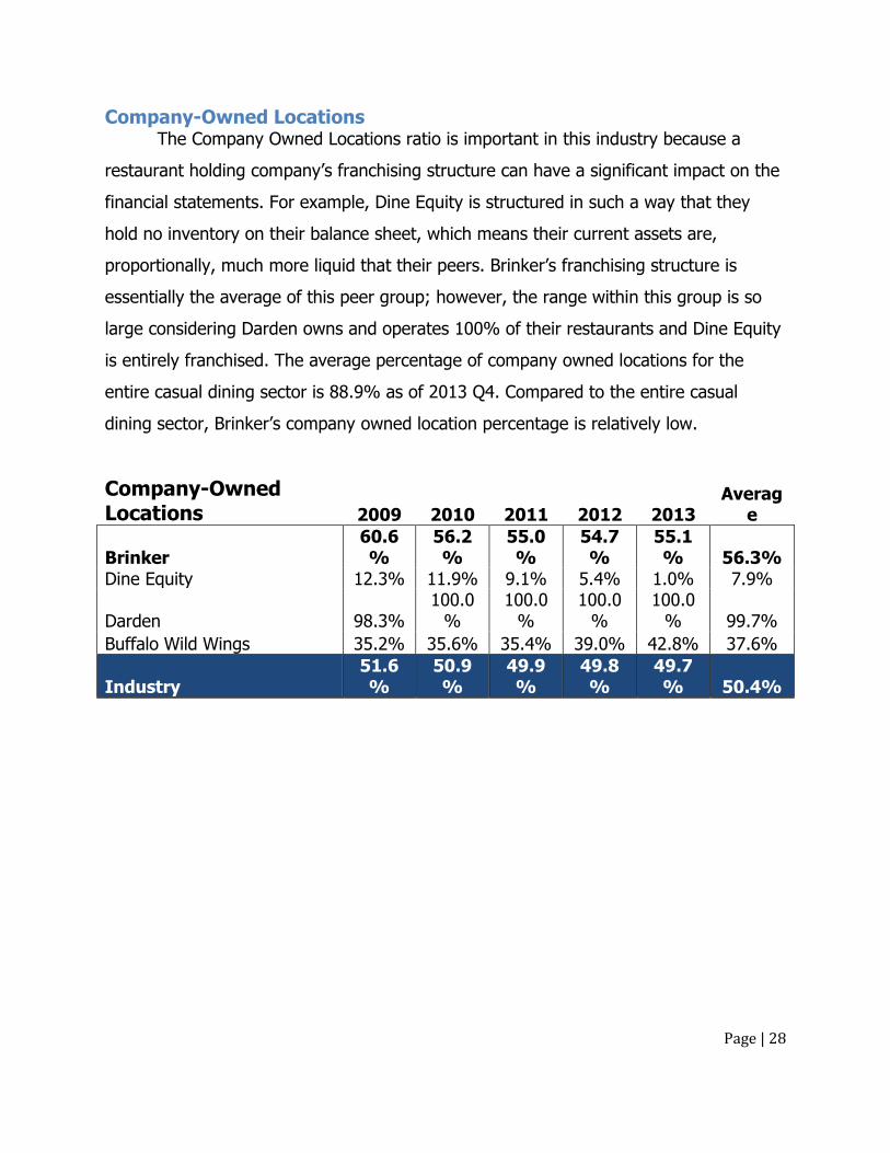
Company-Owned Locations The Company Owned Locations ratio is important in this industry because a
restaurant holding company’s franchising structure can have a significant impact on the
financial statements. For example, Dine Equity is structured in such a way that they
hold no inventory on their balance sheet, which means their current assets are,
proportionally, much more liquid that their peers. Brinker’s franchising structure is
essentially the average of this peer group; however, the range within this group is so
large considering Darden owns and operates 100% of their restaurants and Dine Equity
is entirely franchised. The average percentage of company owned locations for the
entire casual dining sector is 88.9% as of 2013 Q4. Compared to the entire casual
dining sector, Brinker’s company owned location percentage is relatively low.
Company-Owned Locations 2009 2010 2011 2012 2013
Average
Brinker 60.6%
56.2%
55.0%
54.7%
55.1% 56.3%
Dine Equity 12.3% 11.9% 9.1% 5.4% 1.0% 7.9%
Darden 98.3% 100.0
% 100.0
% 100.0
% 100.0
% 99.7%
Buffalo Wild Wings 35.2% 35.6% 35.4% 39.0% 42.8% 37.6%
Industry 51.6%
50.9%
49.9%
49.8%
49.7% 50.4%
Page | 29
Figure 22.
Financial Analysis Conclusion
Brinker’s current financial statements have shown us that, compared to its peers,
is generally less liquid, less profitable, able to sustain less growth moving forward
without adapting.
Financial Forecasting
Financial forecasting is essential to the valuation process. It is important to
make educated assumptions using historical trends, ratios, the current economic
environment, and industry related patterns. Using these methods will help us define
the intrinsic value of the firm. Of course, the longer the forecasted period, the more
unreliable the estimated numbers will become. Using the income statement, balance
sheet, and statement of cash flows of Brinker International, we will forecast out the
next 10 years of financial information.
0.0%
20.0%
40.0%
60.0%
80.0%
100.0%
120.0%
2008 2009 2010 2011 2012 2013 2014
Company Owned Locations
Brinker Dine Equity Darden Buffalo Wild Wings Industry
Page | 30
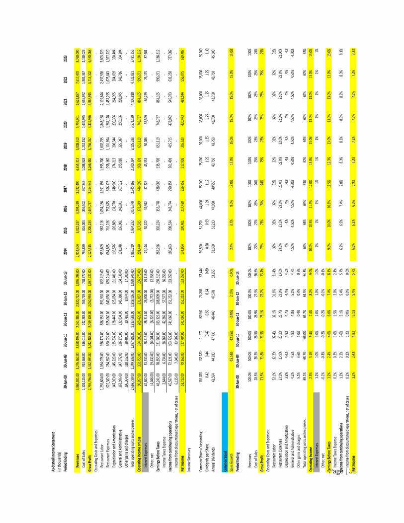
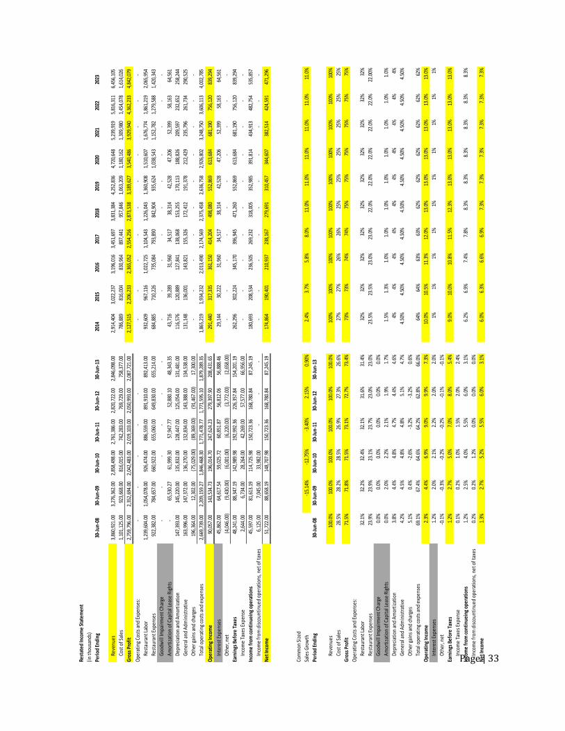
Income Statement The first financial statement to be forecasted is the income statement. The
income statement is important to forecast with logical assumptions because the
numbers used in the balance sheet and statement of cash flows are pulled directly from
it. The most important factor in forecasting the income statement is the sales growth
figure. Future revenues are used in multiple ratios, including liquidity and profitability.
As always, the current economic conditions must also me taken into consideration.
Since we are slowly coming out of the housing recession, the sales growth rate has
been adjusted to take this into account. Brinker International has been showing an
increasing trend in sales over the past 5 years. We have continued this trend, but on a
cautious basis, since the average consumer still seems hesitant about the economic
future. We started with a sales growth of 2.4% in 2014 and continued the upward
trend to a max of 17% in 2018 and finally settling down to 15% in 2019 and on.
After the sales growth is projected, a common sized income statement can be
created. A common size income statement reports line items as a percentage of
revenues. Using this method, trends and patterns are easier to see and easier to
forecast. We have continued Brinker International’s upward trend and have forecasted
their gross profit margin to rise steadily from 73% in 2014 to a maintenance amount of
75% in 2018 and on. This gives us a cost of goods sold of 27% in 2014 and a final
number of 25% in 2018 and thereafter. We have also noticed a trend of Brinker
lowering their restaurant expenses. We have continued this trend by forecasting these
expenses as 23.5% in 2014 and slowly decreasing to 21.5% in 2019 and thereafter.
Following the trend of lower expenses and increasing sales growth, we have naturally
forecasted the operating income, earnings before taxes, and the net income, to
continue this favorable trend. We started with an operating income of 10% in 2014
and gradually increased it to 13% in 2018 and thereafter. The earnings before taxes
number was forecasted at 9% in 2014 and reached a max of 13% in 2019 and
remaining at that rate. And finally we show net income increasing from 6% in 2014 to
7.3% in 2018 and maintaining at that rate. Again, with a long forecast period of 10
Page | 31
years, unexpected factors could affect our projections. Using these forecasted income
statement numbers, we can now forecast the balance sheet, statement of cash flows,
and look at dividends.
Page | 32
As-S
tate
d In
com
e St
atem
ent
(in th
ousa
nds)
Perio
d En
ding
30-Ju
n-08
30-Ju
n-09
30-Ju
n-10
30-Ju
n-11
30-Ju
n-12
30-Ju
n-13
2014
2015
2016
2017
2018
2019
2020
2021
2022
2023
Reve
nues
3,86
0,92
1.00
3,
276,
362.
00
2,85
8,49
8.00
2,
761,
386.
00
2,82
0,72
2.00
2,
846,
098.
00
2,91
4,40
4
3,02
2,23
7
3,29
4,23
9
3,
722,
490
4,35
5,31
3
5,00
8,61
0
5,
759,
901
6,
623,
887
7,
617,
470
8,76
0,09
0
Cost
of S
ales
1,10
1,12
5.00
92
3,66
8.00
816,
015.
00
74
2,28
3.00
769,
729.
00
75
8,37
7.00
786,
889
816,
004
856,
502
96
7,84
7
1,08
8,82
8
1,25
2,15
2
1,
439,
975
1,
655,
972
1,
904,
367
2,19
0,02
3
Gros
s Pro
fit2,
759,
796.
00
2,35
2,69
4.00
2,
042,
483.
00
2,01
9,10
3.00
2,
050,
993.
00
2,08
7,72
1.00
2,
127,
515
2,
206,
233
2,
437,
737
2,75
4,64
2
3,
266,
485
3,
756,
457
4,31
9,92
6
4,96
7,91
5
5,71
3,10
2
6,
570,
068
Oper
atin
g Cos
ts an
d Ex
pens
es:
-
-
-
-
-
-
-
-
-
-
Rest
aura
nt La
bor
1,23
9,60
4.00
1,
054,
078.
00
926,
474.
00
88
6,55
9.00
891,
910.
00
89
2,41
3.00
932,
609
967,
116
1,05
4,15
6
1,
191,
197
1,39
3,70
0
1,60
2,75
5
1,
843,
168
2,
119,
644
2,
437,
590
2,80
3,22
9
Rest
aura
nt Ex
pens
es92
2,38
2.00
784,
657.
00
66
0,92
2.00
655,
060.
00
64
9,83
0.00
655,
214.
00
68
4,88
5
71
0,22
6
75
7,67
5
856,
173
95
8,16
9
1,
101,
894
1,26
7,17
8
1,45
7,25
5
1,67
5,84
3
1,
927,
220
Depr
ecia
tion
and
Amor
tizat
ion
147,
393.
00
14
5,22
0.00
135,
832.
00
12
8,44
7.00
125,
054.
00
13
1,48
1.00
116,
576
120,
889
131,
770
14
8,90
0
174,
213
200,
344
23
0,39
6
26
4,95
5
30
4,69
9
350,
404
Gene
ral a
nd A
dmin
istra
tive
163,
996.
00
14
7,37
2.00
136,
270.
00
13
2,83
4.00
143,
388.
00
13
4,53
8.00
131,
148
136,
001
148,
241
16
7,51
2
195,
989
225,
387
25
9,19
6
29
8,07
5
34
2,78
6
394,
204
Othe
r gai
ns an
d ch
arge
s19
6,36
4.00
118,
612.
00
28
,485
.00
10,7
83.0
0
8,
974.
00
17,3
00.0
0
-
-
-
-
-
-
-
-
-
-
Tota
l ope
ratin
g cos
ts an
d ex
pens
es2,
669,
739.
00
2,24
9,93
9.00
1,
887,
983.
00
1,81
3,68
3.00
1,
819,
156.
00
1,83
0,94
6.00
1,
865,
219
1,
934,
232
2,
075,
370
2,34
5,16
9
2,
700,
294
3,
105,
338
3,57
1,13
9
4,10
6,81
0
4,72
2,83
1
5,
431,
256
Oper
atin
g Inc
ome
or Lo
ss90
,057
.00
102,
755.
00
15
4,50
0.00
205,
420.
00
23
1,83
7.00
256,
775.
00
29
1,44
0
31
7,33
5
37
2,24
9
446,
699
56
6,19
1
65
1,11
9
748,
787
861,
105
990,
271
1,
138,
812
Inte
rest
Expe
nses
45,8
62.0
0
33
,330
.00
28,5
15.0
0
28
,311
.00
26,8
00.0
0
29
,118
.00
29,1
44
30,2
22
32,9
42
37,2
25
43
,553
50
,086
57,5
99
66
,239
76
,175
87,6
01
Othe
r, ne
t(4
,046
.00)
(9,4
30.0
0)
(6
,001
.00)
(6,2
20.0
0)
(3
,772
.00)
(2,6
58.0
0)
-
-
-
-
-
-
-
-
-
-
Earn
ings
Bef
ore
Taxe
s48
,241
.00
78,8
55.0
0
13
1,98
6.00
183,
329.
00
20
8,80
9.00
230,
315.
00
26
2,29
6
30
2,22
4
35
5,77
8
428,
086
53
5,70
3
65
1,11
9
748,
787
861,
105
990,
271
1,
138,
812
Inco
me
Taxe
s Exp
ense
2,64
4.00
6,
734.
00
28,2
64.0
0
42
,269
.00
57,5
77.0
0
66
,956
.00
-
-
-
-
-
-
-
-
-
-
Inco
me
from
cont
inue
ing o
pera
tions
45,5
97.0
0
72
,121
.00
103,
722.
00
14
1,06
0.00
151,
232.
00
16
3,35
9.00
180,
693
208,
534
243,
774
29
0,35
4
361,
491
415,
715
47
8,07
2
54
9,78
3
63
2,25
0
727,
087
Inco
me
from
disc
ount
inue
d op
erat
ions
, net
of t
axes
6,12
5.00
7,
045.
00
33,9
82.0
0
-
-
-
-
-
-
-
-
-
-
-
-
-
Net I
ncom
e51
,722
.00
79,1
66.0
0
13
7,70
4.00
141,
060.
00
15
1,23
2.00
163,
359.
00
17
4,86
4
19
0,40
1
21
7,42
0
256,
852
31
7,93
8
36
5,62
9
420,
473
483,
544
556,
075
63
9,48
7
Inco
me
Sum
mar
y
Com
mon
Shar
es O
utst
andi
ng
101,
320
10
2,12
0
101,
570
8
2,94
0
74,
340
67,4
4459
,500
51
,750
44
,000
35,0
0035
,000
35,0
0035
,000
35,0
0035
,000
35,0
00
Divi
dend
s per
Shar
e0.
420.
440.
470.
560.
640.
800.
880.
991.
091.
171.
251.
251.
251.
251.
251.
30
Annu
al D
ivid
ends
42,5
54
44
,933
47,7
38
46
,446
47,5
78
53
,955
52,3
60
51,2
33
47,9
60
40,9
50
43
,750
43
,750
43,7
50
43
,750
43
,750
45,5
00
Com
mon
Size
d
Sale
s Gro
wth
-15.
14%
-12.
75%
-3.4
0%2.
15%
0.90
%2.
4%3.
7%9.
0%13
.0%
17.0
%15
.0%
15.0
%15
.0%
15.0
%15
.0%
Perio
d En
ding
30-Ju
n-08
30-Ju
n-09
30-Ju
n-10
30-Ju
n-11
30-Ju
n-12
30-Ju
n-13
Reve
nues
100.
0%10
0.0%
100.
0%10
0.0%
100.
0%10
0.0%
100%
100%
100%
100%
100%
100%
100%
100%
100%
100%
Cost
of S
ales
28.5
%28
.2%
28.5
%26
.9%
27.3
%26
.6%
27%
27%
26%
26%
25%
25%
25%
25%
25%
25%
Gros
s Pro
fit71
.5%
71.8
%71
.5%
73.1
%72
.7%
73.4
%73
%73
%74
%74
%75
%75
%75
%75
%75
%75
%
Oper
atin
g Cos
ts an
d Ex
pens
es:
Rest
aura
nt La
bor
32.1
%32
.2%
32.4
%32
.1%
31.6
%31
.4%
32%
32%
32%
32%
32%
32%
32%
32%
32%
32%
Rest
aura
nt Ex
pens
es23
.9%
23.9
%23
.1%
23.7
%23
.0%
23.0
%23
.5%
23.5
%23
.0%
23.0
%22
.0%
22.0
%22
.0%
22.0
%22
.0%
22.0
0%
Depr
ecia
tion
and
Amor
tizat
ion
3.8%
4.4%
4.8%
4.7%
4.4%
4.6%
4%4%
4%4%
4%4%
4%4%
4%4%
Gene
ral a
nd A
dmin
istra
tive
4.2%
4.5%
4.8%
4.8%
5.1%
4.7%
4.50
%4.
50%
4.50
%4.
50%
4.50
%4.
50%
4.50
%4.
50%
4.50
%4.
50%
Othe
r gai
ns an
d ch
arge
s5.
1%3.
6%1.
0%0.
4%0.
3%0.
6%
Tota
l ope
ratin
g cos
ts an
d ex
pens
es69
.1%
68.7
%66
.0%
65.7
%64
.5%
64.3
%64
%64
%63
%63
%62
%62
%62
%62
%62
%62
%
Oper
atin
g Inc
ome
2.3%
3.1%
5.4%
7.4%
8.2%
9.0%
10.0
%10
.5%
11.3
%12
.0%
13.0
%13
.0%
13.0
%13
.0%
13.0
%13
.0%
Inte
rest
Expe
nses
1.2%
1.0%
1.0%
1.0%
1.0%
1.0%
1%1%
1%1%
1%1%
1%1%
1%1%
Othe
r, ne
t-0
.1%
-0.3
%-0
.2%
-0.2
%-0
.1%
-0.1
%
Earn
ings
Bef
ore
Taxe
s1.
2%2.
4%4.
6%6.
6%7.
4%8.
1%9.
0%10
.0%
10.8
%11
.5%
12.3
%13
.0%
13.0
%13
.0%
13.0
%13
.0%
Inco
me
Taxe
s Exp
ense
0.1%
0.2%
1.0%
1.5%
2.0%
2.4%
Inco
me
from
cont
inui
ng o
pera
tions
1.2%
2.2%
3.6%
5.1%
5.4%
5.7%
6.2%
6.9%
7.4%
7.8%
8.3%
8.3%
8.3%
8.3%
8.3%
8.3%
Inco
me
from
disc
ount
inue
d op
erat
ions
, net
of t
axes
0.2%
0.2%
1.2%
0.0%
0.0%
0.0%
Net I
ncom
e1.
3%2.
4%4.
8%5.
1%5.
4%5.
7%6.
0%6.
3%6.
6%6.
9%7.
3%7.
3%7.
3%7.
3%7.
3%7.
3%
Page | 33
Rest
ated
Inco
me
Stat
emen
t
(in
thou
sand
s)
Peri
od E
ndin
g30
-Jun
-08
30-J
un-0
930
-Jun
-10
30-J
un-1
130
-Jun
-12
30-J
un-1
320
1420
1520
1620
1720
1820
1920
2020
2120
2220
23
Reve
nues
3,86
0,92
1.00
3,
276,
362.
00
2,
858,
498.
00
2,76
1,38
6.00
2,
820,
722.
00
2,84
6,09
8.00
2,
914,
404
3,
022,
237
3,19
6,01
6
3,45
1,69
7
3,83
1,38
4
4,
252,
836
4,
720,
648
5,
239,
919
5,81
6,31
1
6,45
6,10
5
Cost
of S
ales
1,10
1,12
5.00
92
3,66
8.00
81
6,01
5.00
742,
283.
00
76
9,72
9.00
758,
377.
00
78
6,88
9
81
6,00
4
830,
964
897,
441
957,
846
1,
063,
209
1,
180,
162
1,
309,
980
1,45
4,07
8
1,61
4,02
6
Gro
ss P
rofi
t2,
759,
796.
00
2,35
2,69
4.00
2,04
2,48
3.00
2,
019,
103.
00
2,05
0,99
3.00
2,
087,
721.
00
2,12
7,51
5
2,20
6,23
3
2,
365,
052
2,
554,
256
2,
873,
538
3,18
9,62
7
3,54
0,48
6
3,92
9,94
0
4,
362,
233
4,
842,
079
Ope
rati
ng C
osts
and
Exp
ense
s:-
-
-
-
-
-
-
-
-
-
-
-
-
-
-
Rest
aura
nt L
abor
1,23
9,60
4.00
1,
054,
078.
00
92
6,47
4.00
886,
559.
00
89
1,91
0.00
892,
413.
00
93
2,60
9
96
7,11
6
1,02
2,72
5
1,10
4,54
3
1,22
6,04
3
1,
360,
908
1,
510,
607
1,
676,
774
1,86
1,21
9
2,06
5,95
4
Rest
aura
nt E
xpen
ses
922,
382.
00
78
4,65
7.00
66
0,92
2.00
655,
060.
00
64
9,83
0.00
655,
214.
00
68
4,88
5
71
0,22
6
735,
084
793,
890
842,
904
93
5,62
4
1,03
8,54
3
1,15
2,78
2
1,
279,
588
1,
420,
343
Goo
dwill
Impa
irm
ent C
harg
e-
-
-
-
-
-
-
-
-
-
-
-
-
-
-
-
Am
orti
zati
on o
f Cap
ital
Lea
se R
ight
s-
65
,530
.27
61,9
99.3
0
57,9
47.7
7
52,8
80.1
0
48,3
43.3
5
43,7
16
39,2
89
31
,960
34
,517
38
,314
42,5
28
47,2
06
52,3
99
58
,163
64
,561
Dep
reci
atio
n an
d A
mor
tiza
tion
147,
393.
00
14
5,22
0.00
13
5,83
2.00
128,
447.
00
12
5,05
4.00
131,
481.
00
11
6,57
6
12
0,88
9
127,
841
138,
068
153,
255
17
0,11
3
188,
826
20
9,59
7
232,
652
258,
244
Gen
eral
and
Adm
inis
trat
ive
163,
996.
00
14
7,37
2.00
13
6,27
0.00
132,
834.
00
14
3,38
8.00
134,
538.
00
13
1,14
8
13
6,00
1
143,
821
155,
326
172,
412
19
1,37
8
212,
429
23
5,79
6
261,
734
290,
525
Oth
er g
ains
and
cha
rges
196,
364.
00
12
,302
.00
(75,
029.
00)
(89,
369.
00)
(91,
467.
00)
17,3
00.0
0
-
-
-
-
-
-
-
-
-
-
Tota
l ope
rati
ng c
osts
and
exp
ense
s2,
669,
739.
00
2,20
9,15
9.27
1,84
6,46
8.30
1,
771,
478.
77
1,77
1,59
5.10
1,
879,
289.
35
1,86
5,21
9
1,93
4,23
2
2,
013,
490
2,
174,
569
2,
375,
458
2,63
6,75
8
2,92
6,80
2
3,24
8,75
0
3,
606,
113
4,
002,
785
Ope
rati
ng In
com
e90
,057
.00
14
3,53
4.73
19
6,01
4.70
247,
624.
23
27
9,39
7.90
208,
431.
65
29
1,44
0
31
7,33
5
361,
150
414,
204
498,
080
55
2,86
9
613,
684
68
1,19
0
756,
120
839,
294
Inte
rest
Exp
ense
s45
,862
.00
64
,617
.54
59,0
25.7
2
60,8
51.8
7
56,8
12.0
6
56,8
88.4
6
29,1
44
30,2
22
31
,960
34
,517
38
,314
42,5
28
47,2
06
52,3
99
58
,163
64
,561
Oth
er, n
et(4
,046
.00)
(9
,430
.00)
(6,0
01.0
0)
(6,2
20.0
0)
(3,7
72.0
0)
(2,6
58.0
0)
-
-
-
-
-
-
-
-
-
-
Earn
ings
Bef
ore
Taxe
s48
,241
.00
88
,347
.19
142,
989.
98
19
2,99
2.36
226,
357.
84
15
4,20
1.19
262,
296
302,
224
34
5,17
0
39
6,94
5
47
1,26
0
552,
869
61
3,68
4
681,
190
75
6,12
0
83
9,29
4
Inco
me
Taxe
s Ex
pens
e2,
644.
00
6,
734.
00
28
,264
.00
42
,269
.00
57
,577
.00
66
,956
.00
-
-
-
-
-
-
-
-
-
-
Inco
me
from
con
tinu
eing
ope
rati
ons
45,5
97.0
0
81,6
13.1
9
11
4,72
5.98
150,
723.
36
16
8,78
0.84
87,2
45.1
9
180,
693
208,
534
23
6,50
5
26
9,23
2
31
8,00
5
352,
985
39
1,81
4
434,
913
48
2,75
4
53
5,85
7
Inco
me
from
dis
coun
tinu
ed o
pera
tion
s, n
et o
f tax
es6,
125.
00
7,
045.
00
33
,982
.00
-
-
-
-
-
-
-
-
-
-
-
-
-
Net
Inco
me
51,7
22.0
0
88,6
58.1
9
14
8,70
7.98
150,
723.
36
16
8,78
0.84
87,2
45.1
9
174,
864
190,
401
21
0,93
7
23
8,16
7
27
9,69
1
310,
457
34
4,60
7
382,
514
42
4,59
1
47
1,29
6
Com
mon
Siz
ed
Sale
s G
row
th-1
5.14
%-1
2.75
%-3
.40%
2.15
%0.
90%
2.4%
3.7%
5.8%
8.0%
11.0
%11
.0%
11.0
%11
.0%
11.0
%11
.0%
Peri
od E
ndin
g30
-Jun
-08
30-J
un-0
930
-Jun
-10
30-J
un-1
130
-Jun
-12
30-J
un-1
3
Reve
nues
100.
0%10
0.0%
100.
0%10
0.0%
100.
0%10
0.0%
100%
100%
100%
100%
100%
100%
100%
100%
100%
100%
Cost
of S
ales
28.5
%28
.2%
28.5
%26
.9%
27.3
%26
.6%
27%
27%
26%
26%
25%
25%
25%
25%
25%
25%
Gro
ss P
rofi
t71
.5%
71.8
%71
.5%
73.1
%72
.7%
73.4
%73
%73
%74
%74
%75
%75
%75
%75
%75
%75
%
Ope
rati
ng C
osts
and
Exp
ense
s:
Rest
aura
nt L
abor
32.1
%32
.2%
32.4
%32
.1%
31.6
%31
.4%
32%
32%
32%
32%
32%
32%
32%
32%
32%
32%
Rest
aura
nt E
xpen
ses
23.9
%23
.9%
23.1
%23
.7%
23.0
%23
.0%
23.5
%23
.5%
23.0
%23
.0%
22.0
%22
.0%
22.0
%22
.0%
22.0
%22
.00%
Goo
dwill
Impa
irm
ent C
harg
e0.
0%0.
0%0.
0%0.
0%0.
0%0.
0%
Am
orti
zati
on o
f Cap
ital
Lea
se R
ight
s0.
0%2.
0%2.
2%2.
1%1.
9%1.
7%1.
5%1.
3%1.
0%1.
0%1.
0%1.
0%1.
0%1.
0%1.
0%1.
0%
Dep
reci
atio
n an
d A
mor
tiza
tion
3.8%
4.4%
4.8%
4.7%
4.4%
4.6%
4%4%
4%4%
4%4%
4%4%
4%4%
Gen
eral
and
Adm
inis
trat
ive
4.2%
4.5%
4.8%
4.8%
5.1%
4.7%
4.50
%4.
50%
4.50
%4.
50%
4.50
%4.
50%
4.50
%4.
50%
4.50
%4.
50%
Oth
er g
ains
and
cha
rges
5.1%
0.4%
-2.6
%-3
.2%
-3.2
%0.
6%
Tota
l ope
rati
ng c
osts
and
exp
ense
s69
.1%
67.4
%64
.6%
64.2
%62
.8%
66.0
%64
%64
%63
%63
%62
%62
%62
%62
%62
%62
%
Ope
rati
ng In
com
e2.
3%4.
4%6.
9%9.
0%9.
9%7.
3%10
.0%
10.5
%11
.3%
12.0
%13
.0%
13.0
%13
.0%
13.0
%13
.0%
13.0
%
Inte
rest
Exp
ense
s1.
2%2.
0%2.
1%2.
2%2.
0%2.
0%1%
1%1%
1%1%
1%1%
1%1%
1%
Oth
er, n
et-0
.1%
-0.3
%-0
.2%
-0.2
%-0
.1%
-0.1
%
Earn
ings
Bef
ore
Taxe
s1.
2%2.
7%5.
0%7.
0%8.
0%5.
4%9.
0%10
.0%
10.8
%11
.5%
12.3
%13
.0%
13.0
%13
.0%
13.0
%13
.0%
Inco
me
Taxe
s Ex
pens
e0.
1%0.
2%1.
0%1.
5%2.
0%2.
4%
Inco
me
from
con
tinu
eing
ope
rati
ons
1.2%
2.5%
4.0%
5.5%
6.0%
3.1%
6.2%
6.9%
7.4%
7.8%
8.3%
8.3%
8.3%
8.3%
8.3%
8.3%
Inco
me
from
dis
coun
tinu
ed o
pera
tion
s, n
et o
f tax
es0.
2%0.
2%1.
2%0.
0%0.
0%0.
0%
Net
Inco
me
1.3%
2.7%
5.2%
5.5%
6.0%
3.1%
6.0%
6.3%
6.6%
6.9%
7.3%
7.3%
7.3%
7.3%
7.3%
7.3%
Page | 34
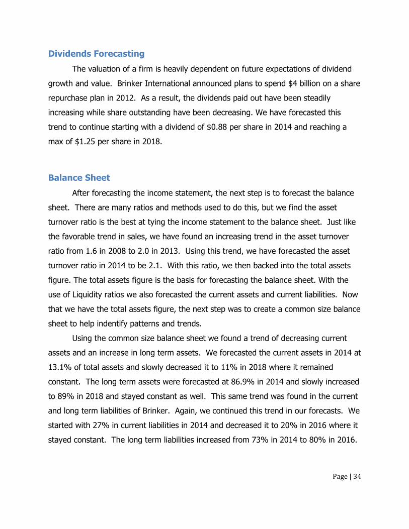
Dividends Forecasting
The valuation of a firm is heavily dependent on future expectations of dividend
growth and value. Brinker International announced plans to spend $4 billion on a share
repurchase plan in 2012. As a result, the dividends paid out have been steadily
increasing while share outstanding have been decreasing. We have forecasted this
trend to continue starting with a dividend of $0.88 per share in 2014 and reaching a
max of $1.25 per share in 2018.
Balance Sheet
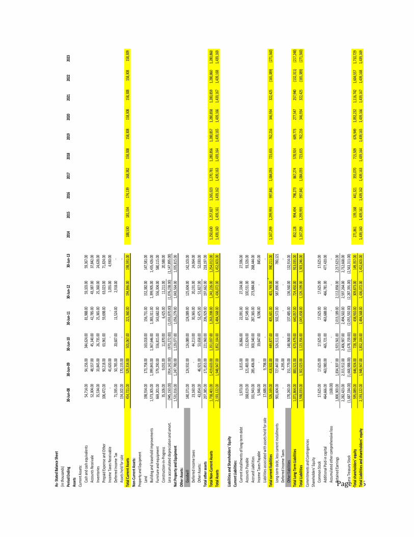
After forecasting the income statement, the next step is to forecast the balance
sheet. There are many ratios and methods used to do this, but we find the asset
turnover ratio is the best at tying the income statement to the balance sheet. Just like
the favorable trend in sales, we have found an increasing trend in the asset turnover
ratio from 1.6 in 2008 to 2.0 in 2013. Using this trend, we have forecasted the asset
turnover ratio in 2014 to be 2.1. With this ratio, we then backed into the total assets
figure. The total assets figure is the basis for forecasting the balance sheet. With the
use of Liquidity ratios we also forecasted the current assets and current liabilities. Now
that we have the total assets figure, the next step was to create a common size balance
sheet to help indentify patterns and trends.
Using the common size balance sheet we found a trend of decreasing current
assets and an increase in long term assets. We forecasted the current assets in 2014 at
13.1% of total assets and slowly decreased it to 11% in 2018 where it remained
constant. The long term assets were forecasted at 86.9% in 2014 and slowly increased
to 89% in 2018 and stayed constant as well. This same trend was found in the current
and long term liabilities of Brinker. Again, we continued this trend in our forecasts. We
started with 27% in current liabilities in 2014 and decreased it to 20% in 2016 where it
stayed constant. The long term liabilities increased from 73% in 2014 to 80% in 2016.

Page | 35
The trends we are finding in Brinker match the trends of the casual dining industry, as
well as, the slowly improving economy.
Page | 36
As- S
tate
d Ba
lanc
e Sh
eet
(in th
ousa
nds)
Perio
d En
ding
30
-Jun
-08
30-J
un-0
930
-Jun
-10
30-J
un-1
130
-Jun
-12
30-J
un-1
320
1420
1520
1620
1720
1820
1920
2020
2120
2220
23
Asse
ts
Curr
ent A
sset
s:
Cash
and
cash
equ
ival
ents
54,7
14.0
0
94
,156
.00
344,
624.
00
81,9
88.0
0
59
,103
.00
59,3
67.0
0
Acco
unts
Rec
eiva
le
52,3
04.0
0
48
,557
.00
45,1
40.0
0
42
,785
.00
43,3
87.0
0
37
,842
.00
Inve
ntor
ies
35,5
34.0
0
33
,845
.00
26,7
35.0
0
25
,365
.00
25,3
60.0
0
24
,628
.00
Prep
aid
Expe
nse
and
Oth
er10
6,47
2.00
90
,218
.00
63,9
61.0
0
59
,698
.00
63,0
23.0
0
71
,824
.00
Inco
me
Taxe
s Rec
eiva
ble
-
41,6
20.0
0
-
-
1,
055.
00
4,
930.
00
Defe
rred
Inco
me
Tax
71,5
95.0
0
50
,785
.00
20,6
07.0
0
11
,524
.00
2,91
8.00
-
Asse
ts h
eld
for s
ale
134,
102.
00
170,
133.
00
-
-
Tota
l Cur
rent
Ass
ets
454,
721.
00
529,
314.
00
501,
067.
00
221,
360.
00
194,
846.
00
198,
591.
00
188,
530
181,
334
174,
139
168,
382
158,
308
158,
308
158,
308
158,
308
158,
308
158,
309
Non
-Cur
rent
Ass
ets:
Prop
erty
and
Equ
ipm
ent
Land
19
8,55
4.00
17
3,75
8.00
16
3,01
8.00
15
6,73
1.00
15
2,38
2.00
14
7,58
1.00
Build
ing
and
leas
ehol
d im
prov
emen
ts1,
573,
305.
00
1,
399,
843.
00
1,
367,
646.
00
1,
383,
311.
00
1,39
9,90
5.00
1,43
5,42
6.00
Furn
iture
and
equ
ipm
ent
669,
201.
00
579,
290.
00
556,
815.
00
543,
682.
00
556,
304.
00
580,
115.
00
Cons
truc
tion-
in-P
rogr
ess
35,1
06.0
0
9,
031.
00
11
,870
.00
6,42
5.00
11
,211
.00
20,5
88.0
0
Less
acc
umul
ated
dep
reci
atio
n an
d am
ort.
(945
,150
.00)
(9
14,1
42.0
0)
(970
,272
.00)
(1
,033
,870
.00)
(1,0
76,2
38.0
0)
(1
,147
,895
.00)
Net
Pro
pert
y an
d Eq
uipm
ent
1,53
1,01
6.00
1,24
7,78
0.00
1,12
9,07
7.00
1,05
6,27
9.00
1,
043,
564.
00
1,
035,
815.
00
Oth
er A
sset
s:
Good
will
140,
371.
00
124,
932.
00
124,
089.
00
124,
089.
00
125,
604.
00
142,
103.
00
Defe
rred
inco
me
taxe
s23
,160
.00
-
44,2
13.0
0
30
,365
.00
20,2
31.0
0
24
,064
.00
Oth
er A
sset
s:43
,854
.00
46,9
21.0
0
53
,658
.00
52,4
75.0
0
51
,827
.00
52,0
30.0
0
Tota
l oth
er a
sset
s20
7,38
5.00
17
1,85
3.00
22
1,96
0.00
20
6,92
9.00
19
7,66
2.00
21
8,19
7.00
Tota
l Non
-Cur
rent
Ass
ets
1,73
8,40
1.00
1,41
9,63
3.00
1,35
1,03
7.00
1,26
3,20
8.00
1,
241,
226.
00
1,
254,
012.
00
1,
250,
630
1,25
7,82
7
1,
265,
023
1,27
0,78
1
1,
280,
856
1,28
0,85
7
1,
280,
858
1,28
0,85
9
1,
280,
860
1,28
0,86
0
Tota
l Ass
ets
2,19
3,12
2.00
1,94
8,94
7.00
1,85
2,10
4.00
1,48
4,56
8.00
1,
436,
072.
00
1,
452,
603.
00
1,
439,
160
1,43
9,16
1
1,
439,
162
1,43
9,16
3
1,
439,
164
1,43
9,16
5
1,
439,
166
1,43
9,16
7
1,
439,
168
1,43
9,16
9
Liab
ilitie
s and
Sha
reho
lder
s' E
quity
Curr
ent L
iabi
litie
s:
Curr
ent i
nsta
llmen
ts o
f lon
g-te
rm d
ebt
1,97
3.00
1,81
5.00
16,8
66.0
0
22
,091
.00
27,3
34.0
0
27
,596
.00
Acco
unts
Pay
able
168,
619.
00
121,
483.
00
112,
824.
00
87,5
49.0
0
10
0,53
1.00
93
,326
.00
Accr
ued
Liab
ilitie
s 33
1,94
3.00
28
5,40
6.00
30
0,54
0.00
28
7,36
5.00
27
3,88
4.00
26
8,44
4.00
Inco
me
Taxe
s Pay
able
5,94
6.00
-
19,6
47.0
0
8,
596.
00
-
845.
00
Liab
ilitie
s ass
ocia
ted
with
ass
ets h
eld
for s
ale
17,6
88.0
0
9,
798.
00
-
-
Tota
l cur
rent
liab
ilitie
s52
6,16
9.00
41
8,50
2.00
44
9,87
7.00
40
5,60
1.00
40
1,74
9.00
39
0,21
1.00
1,
167,
299
1,29
9,99
3
99
7,84
1
1,
084,
093
723,
655
762,
216
346,
934
322,
425
(165
,389
)
(2
71,5
60)
Long
-ter
m d
ebt,
less
curr
ent i
nsta
llmen
ts90
1,60
4.00
72
7,44
7.00
52
4,51
1.00
50
2,57
2.00
58
7,89
0.00
78
0,12
1
Defe
rred
Inco
me
Taxe
s-
4,
295.
00
-
-
-
-
Oth
er li
abili
ties
170,
260.
00
151,
779.
00
148,
968.
00
137,
485.
00
136,
560.
00
132,
914.
00
Tota
l Lon
g-Te
rm Li
abili
ties
1,07
1,86
4.00
883,
521.
00
673,
479.
00
640,
057.
00
724,
450.
00
913,
035.
00
852,
128
994,
494
798,
273
867,
274
578,
924
609,
773
277,
547
257,
940
(132
,311
)
(2
17,2
48)
Tota
l Lia
bilit
ies
1,59
8,03
3.00
1,30
2,02
3.00
1,12
3,35
6.00
1,04
5,65
8.00
1,
126,
199.
00
1,
303,
246.
00
1,
167,
299
1,29
9,99
3
99
7,84
1
1,
084,
093
723,
655
762,
216
346,
934
322,
425
(165
,389
)
(2
71,5
60)
Com
mitm
ents
and
Con
tinge
ncie
s
Shar
ehol
ders
' Equ
ity
Com
mon
Sto
ck17
,625
.00
17,6
25.0
0
17
,625
.00
17,6
25.0
0
17
,625
.00
17,6
25.0
0
Addi
tiona
l Pai
d-in
capi
tal
464,
666.
00
463,
980.
00
465,
721.
00
463,
688.
00
466,
781.
00
477,
420.
00
Accu
mul
ated
oth
er co
mpr
ehen
sive
loss
(168
.00)
-
-
-
-
-
Reta
ined
Ear
ning
s1,
800,
300.
00
1,
834,
307.
00
1,
923,
561.
00
2,
013,
189.
00
2,11
2,85
8.00
2,21
7,62
3.00
2,28
2,42
3.00
2,31
5,91
2.00
2,40
6,90
7.00
2,49
4,50
2.00
2,
597,
264.
00
2,
712,
668.
00
Less
Tre
asur
y St
ock
(1,6
87,3
34.0
0)
(1
,668
,988
.00)
(1,6
78,1
59.0
0)
(2
,055
,592
.00)
(2,2
87,3
91.0
0)
(2
,563
,311
.00)
Tota
l sha
reho
lder
s' e
quity
595,
089.
00
646,
924.
00
728,
748.
00
438,
910.
00
309,
873.
00
149,
357.
00
271,
861
139,
168
441,
321
355,
070
715,
509
676,
949
1,09
2,23
2
1,
116,
742
1,60
4,55
7
1,
710,
729
Tota
l Lia
bilit
ies a
nd sh
areh
olde
rs' e
quity
2,19
3,12
2.00
1,94
8,94
7.00
1,85
2,10
4.00
1,48
4,56
8.00
1,
436,
072.
00
1,
452,
603.
00
1,
439,
160
1,43
9,16
1
1,
439,
162
1,43
9,16
3
1,
439,
164
1,43
9,16
5
1,
439,
166
1,43
9,16
7
1,
439,
168
1,43
9,16
9
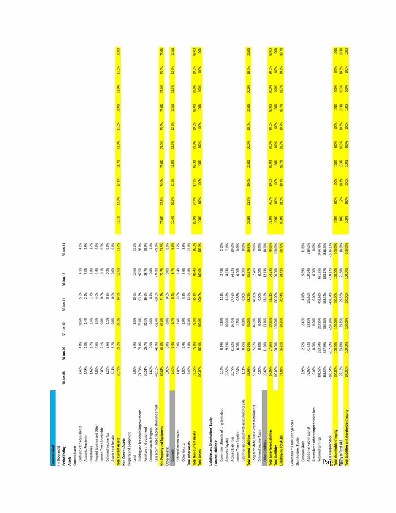
Page | 37
Com
mon
Siz
ed
(in th
ousa
nds)
Perio
d En
ding
30
-Jun
-08
30-J
un-0
930
-Jun
-10
30-J
un-1
130
-Jun
-12
30-J
un-1
3
Asse
ts
Curr
ent A
sset
s:
Cash
and
cash
equ
ival
ents
2.49
%4.
8%18
.6%
5.5%
4.1%
4.1%
Acco
unts
Rec
eiva
le
2.38
%2.
5%2.
4%2.
9%3.
0%2.
6%
Inve
ntor
ies
1.62
%1.
7%1.
4%1.
7%1.
8%1.
7%
Prep
aid
Expe
nse
and
Oth
er4.
85%
4.6%
3.5%
4.0%
4.4%
4.9%
Inco
me
Taxe
s Rec
eiva
ble
0.00
%2.
1%0.
0%0.
0%0.
1%0.
3%
Defe
rred
Inco
me
Tax
3.26
%2.
6%1.
1%0.
8%0.
2%0.
0%
Asse
ts h
eld
for s
ale
6.11
%8.
7%0.
0%0.
0%0.
0%0.
0%
Tota
l Cur
rent
Ass
ets
20.7
3%27
.2%
27.1
%14
.9%
13.6
%13
.7%
13.1
%12
.6%
12.1
%11
.7%
11.0
%11
.0%
11.0
%11
.0%
11.0
%11
.0%
Non
-Cur
rent
Ass
ets:
Prop
erty
and
Equ
ipm
ent
Land
9.
05%
8.9%
8.8%
10.6
%10
.6%
10.2
%
Build
ing
and
leas
ehol
d im
prov
emen
ts71
.74%
71.8
%73
.8%
93.2
%97
.5%
98.8
%
Furn
iture
and
equ
ipm
ent
30.5
1%29
.7%
30.1
%36
.6%
38.7
%39
.9%
Cons
truc
tion-
in-P
rogr
ess
1.60
%0.
5%0.
6%0.
4%0.
8%1.
4%
Less
acc
umul
ated
dep
reci
atio
n an
d am
ort.
-43.
10%
-46.
9%-5
2.4%
-69.
6%-7
4.9%
-79.
0%
Net
Pro
pert
y an
d Eq
uipm
ent
69.8
1%64
.0%
61.0
%71
.2%
72.7
%71
.3%
72.0
%72
.6%
74.0
%75
.0%
75.0
%75
.0%
75.0
%75
.0%
75.0
%75
.0%
Oth
er A
sset
s:0.
00%
0.0%
0.0%
0.0%
0.0%
0.0%
Good
will
6.40
%6.
4%6.
7%8.
4%8.
7%9.
8%10
.4%
10.9
%11
.5%
12.0
%12
.5%
12.5
%12
.5%
12.5
%12
.5%
12.5
%
Defe
rred
inco
me
taxe
s1.
06%
0.0%
2.4%
2.0%
1.4%
1.7%
Oth
er A
sset
s:2.
00%
2.4%
2.9%
3.5%
3.6%
3.6%
Tota
l oth
er a
sset
s9.
46%
8.8%
12.0
%13
.9%
13.8
%15
.0%
Tota
l Non
-Cur
rent
Ass
ets
79.2
7%72
.8%
72.9
%85
.1%
86.4
%86
.3%
86.9
%87
.4%
87.9
%88
.3%
89.0
%89
.0%
89.0
%89
.0%
89.0
%89
.0%
Tota
l Ass
ets
100.
00%
100.
0%10
0.0%
100.
0%10
0.0%
100.
0%10
0%10
0%10
0%10
0%10
0%10
0%10
0%10
0%10
0%10
0%
Liab
ilitie
s and
Sha
reho
lder
s' E
quity
Curr
ent L
iabi
litie
s:
Curr
ent i
nsta
llmen
ts o
f lon
g-te
rm d
ebt
0.12
%0.
14%
1.50
%2.
11%
2.43
%2.
12%
Acco
unts
Pay
able
10.5
5%9.
33%
10.0
4%8.
37%
8.93
%7.
16%
Accr
ued
Liab
ilitie
s 20
.77%
21.9
2%26
.75%
27.4
8%24
.32%
20.6
0%
Inco
me
Taxe
s Pay
able
0.37
%0.
00%
1.75
%0.
82%
0.00
%0.
06%
Liab
ilitie
s ass
ocia
ted
with
ass
ets h
eld
for s
ale
1.11
%0.
75%
0.00
%0.
00%
0.00
%0.
00%
Tota
l cur
rent
liab
ilitie
s32
.93%
32.1
4%40
.05%
38.7
9%35
.67%
29.9
4%27
.0%
23.5
%20
.0%
20.0
%20
.0%
20.0
%20
.0%
20.0
%20
.0%
20.0
%
Long
-ter
m d
ebt,
less
curr
ent i
nsta
llmen
ts56
.42%
55.8
7%46
.69%
48.0
6%52
.20%
59.8
6%
Defe
rred
Inco
me
Taxe
s0.
00%
0.33
%0.
00%
0.00
%0.
00%
0.00
%
Oth
er li
abili
ties
10.6
5%11
.66%
13.2
6%13
.15%
12.1
3%10
.20%
Tota
l Lon
g-Te
rm Li
abili
ties
67.0
7%67
.86%
59.9
5%61
.21%
64.3
3%70
.06%
73.0
%76
.5%
80.0
%80
.0%
80.0
%80
.0%
80.0
%80
.0%
80.0
%80
.0%
Tota
l Lia
bilit
ies
100.
00%
100.
00%
100.
00%
100.
00%
100.
00%
100.
00%
100%
100%
100%
100%
100%
100%
100%
100%
100%
100%
Liab
ilitie
s to
Tota
l L&
E72
.87%
66.8
1%60
.65%
70.4
4%78
.42%
89.7
2%90
.0%
88.0
%89
.7%
89.7
%89
.7%
89.7
%89
.7%
89.7
%89
.7%
89.7
%
Com
mitm
ents
and
Con
tinge
ncie
s
Shar
ehol
ders
' Equ
ity
Com
mon
Sto
ck2.
96%
2.72
%2.
42%
4.02
%5.
69%
11.8
0%
Addi
tiona
l Pai
d-in
capi
tal
78.0
8%71
.72%
63.9
1%10
5.65
%15
0.64
%31
9.65
%
Accu
mul
ated
oth
er co
mpr
ehen
sive
loss
-0.0
3%0.
00%
0.00
%0.
00%
0.00
%0.
00%
Reta
ined
Ear
ning
s30
2.53
%28
3.54
%26
3.95
%45
8.68
%68
1.85
%14
84.7
8%
383.
54%
357.
99%
330.
28%
568.
34%
838.
17%
1816
.23%
Less
Tre
asur
y St
ock
-283
.54%
-257
.99%
-230
.28%
-468
.34%
-738
.17%
-171
6.23
%
Tota
l sha
reho
lder
s' e
quity
100.
00%
100.
00%
100.
00%
100.
00%
100.
00%
100.
00%
100%
100%
100%
100%
100%
100%
100%
100%
100%
100%
Equi
ty to
Tot
al L&
E27
.13%
33.1
9%39
.35%
29.5
6%21
.58%
10.2
8%10
%12
%10
.3%
10.3
%10
.3%
10.3
%10
.3%
10.3
%10
.3%
10.3
%
Tota
l Lia
bilit
ies a
nd sh
areh
olde
rs' e
quity
100.
00%
100.
00%
100.
00%
100.
00%
100.
00%
100.
00%
100%
100%
100%
100%
100%
100%
100%
100%
100%
100%
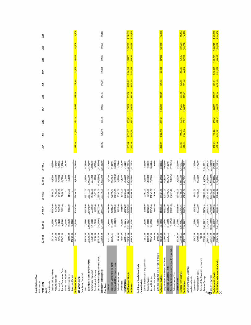
Page | 38
Rest
ated
Bal
ance
She
et
(in th
ousa
nds)
Perio
d En
ding
30
-Jun
-08
30-J
un-0
930
-Jun
-10
30-J
un-1
130
-Jun
-12
30-J
un-1
320
1420
1520
1620
1720
1820
1920
2020
2120
2220
23
Asse
ts
Curr
ent A
sset
s:
Cash
and
cash
equ
ival
ents
54,7
14.0
0
94,1
56.0
0
34
4,62
4.00
81
,988
.00
59,1
03.0
0
59
,367
.00
Acco
unts
Rec
eiva
le
52,3
04.0
0
48,5
57.0
0
45
,140
.00
42
,785
.00
43,3
87.0
0
37
,842
.00
Inve
ntor
ies
35,5
34.0
0
33,8
45.0
0
26
,735
.00
25
,365
.00
25,3
60.0
0
24
,628
.00
Prep
aid
Expe
nse
and
Oth
er10
6,47
2.00
90,2
18.0
0
63
,961
.00
59
,698
.00
63,0
23.0
0
71
,824
.00
Inco
me
Taxe
s Rec
eiva
ble
-
41
,620
.00
-
-
1,05
5.00
4,93
0.00
Defe
rred
Inco
me
Tax
71,5
95.0
0
50,7
85.0
0
20
,607
.00
11
,524
.00
2,91
8.00
-
Asse
ts h
eld
for s
ale
134,
102.
00
17
0,13
3.00
-
-
-
-
Tota
l Cur
rent
Ass
ets
454,
721.
00
52
9,31
4.00
50
1,06
7.00
22
1,36
0.00
19
4,84
6.00
19
8,59
1.00
18
8,53
0
181,
334
17
4,13
9
168,
382
15
8,30
8
158,
308
15
8,30
8
158,
308
15
8,30
8
158,
309
Non
-Cur
rent
Ass
ets:
Prop
erty
and
Equ
ipm
ent
Land
19
8,55
4.00
173,
758.
00
163,
018.
00
156,
731.
00
152,
382.
00
147,
581.
00
Build
ing
and
leas
ehol
d im
prov
emen
ts1,
573,
305.
00
1,39
9,84
3.00
1,36
7,64
6.00
1,38
3,31
1.00
1,39
9,90
5.00
1,43
5,42
6.00
Furn
iture
and
equ
ipm
ent
669,
201.
00
57
9,29
0.00
55
6,81
5.00
54
3,68
2.00
55
6,30
4.00
58
0,11
5.00
Cons
truc
tion-
in-P
rogr
ess
35,1
06.0
0
9,03
1.00
11,8
70.0
0
6,42
5.00
11
,211
.00
20,5
88.0
0
Less
acc
umul
ated
dep
reci
atio
n an
d am
ort.
(945
,150
.00)
(914
,142
.00)
(9
70,2
72.0
0)
(1
,033
,870
.00)
(1,0
76,2
38.0
0)
(1
,147
,895
.00)
Net
Pro
pert
y an
d Eq
uipm
ent
1,53
1,01
6.00
1,
247,
780.
00
1,
129,
077.
00
1,
056,
279.
00
1,
043,
564.
00
1,
035,
815.
00
81
8,88
2
826,
078
83
3,27
5
839,
032
84
9,10
7
849,
107
84
9,10
8
849,
109
84
9,10
9
849,
110
Oth
er A
sset
s:
Good
will
140,
371.
00
12
4,93
2.00
12
4,08
9.00
12
4,08
9.00
12
5,60
4.00
14
2,10
3.00
Capi
taliz
ed O
pera
ting
Leas
e Ri
ghts
655,
302.
66
55
7,99
3.69
46
3,58
2.19
42
3,04
0.76
38
6,74
6.78
37
6,85
7.91
Accu
mul
ated
Impa
irmen
t of L
ease
-
(6
5,53
0.27
)
(61,
999.
30)
(5
7,94
7.77
)
(5
2,88
0.10
)
(48,
343.
35)
Defe
rred
inco
me
taxe
s23
,160
.00
-
44
,213
.00
30
,365
.00
20,2
31.0
0
24
,064
.00
Oth
er A
sset
s:43
,854
.00
46
,921
.00
53,6
58.0
0
52,4
75.0
0
51
,827
.00
52,0
30.0
0
Tota
l oth
er a
sset
s86
2,68
7.66
664,
316.
43
623,
542.
89
572,
021.
99
531,
528.
69
546,
711.
56
Tota
l Non
-Cur
rent
Ass
ets
2,39
3,70
3.66
1,
912,
096.
43
1,
752,
619.
89
1,
628,
300.
99
1,
575,
092.
69
1,
582,
526.
56
1,
250,
630
1,25
7,82
7
1,
265,
023
1,27
0,78
1
1,
280,
856
1,28
0,85
7
1,
280,
858
1,28
0,85
9
1,
280,
860
1,28
0,86
0
Tota
l Ass
ets
2,84
8,42
4.66
2,
441,
410.
43
2,
253,
686.
89
1,
849,
660.
99
1,
769,
938.
69
1,
781,
117.
56
1,
439,
160
1,43
9,16
1
1,
439,
162
1,43
9,16
3
1,
439,
164
1,43
9,16
5
1,
439,
166
1,43
9,16
7
1,
439,
168
1,43
9,16
9
Liab
ilitie
s and
Sha
reho
lder
s' E
quity
Curr
ent L
iabi
litie
s:
Curr
ent i
nsta
llmen
ts o
f lon
g-te
rm d
ebt
1,97
3.00
1,
815.
00
16
,866
.00
22
,091
.00
27,3
34.0
0
27
,596
.00
Acco
unts
Pay
able
168,
619.
00
12
1,48
3.00
11
2,82
4.00
87
,549
.00
100,
531.
00
93,3
26.0
0
Accr
ued
Liab
ilitie
s 33
1,94
3.00
285,
406.
00
300,
540.
00
287,
365.
00
273,
884.
00
268,
444.
00
Inco
me
Taxe
s Pay
able
5,94
6.00
-
19
,647
.00
8,
596.
00
-
845.
00
Liab
ilitie
s ass
ocia
ted
with
ass
ets h
eld
for s
ale
17,6
88.0
0
9,79
8.00
-
-
-
-
Tota
l cur
rent
liab
ilitie
s52
6,16
9.00
418,
502.
00
449,
877.
00
405,
601.
00
401,
749.
00
390,
211.
00
1,17
2,05
9
1,
306,
720
1,00
8,32
1
1,
095,
370
735,
885
77
5,24
4
360,
914
33
7,20
2
(149
,659
)
(2
56,7
83)
Long
-ter
m d
ebt,
less
curr
ent i
nsta
llmen
ts90
1,60
4.00
727,
447.
00
524,
511.
00
502,
572.
00
587,
890.
00
780,
121.
00
Capi
taliz
ed O
p. Le
ase
Liab
ility
655,
302.
66
55
7,99
3.69
46
3,58
2.19
42
3,04
0.76
38
6,74
6.78
37
6,85
7.91
Accu
,. Re
duct
ion
in P
rinci
pal o
n Ca
p. O
p. Le
ase
Liab
. -
(75,
022.
46)
(7
3,00
3.28
)
(67,
611.
13)
(70,
428.
94)
(7
2,51
6.54
)
Defe
rred
Inco
me
Taxe
s-
4,29
5.00
-
-
-
-
Oth
er li
abili
ties
170,
260.
00
15
1,77
9.00
14
8,96
8.00
13
7,48
5.00
13
6,56
0.00
13
2,91
4.00
Tota
l Lon
g-Te
rm Li
abili
ties
1,72
7,16
6.66
1,
366,
492.
23
1,
064,
057.
91
99
5,48
6.63
1,
040,
767.
85
1,
217,
376.
37
85
5,60
3
999,
641
80
6,65
7
876,
296
58
8,70
8
620,
195
28
8,73
1
269,
762
(1
19,7
27)
(205
,426
)
Tota
l Lia
bilit
ies
2,25
3,33
5.66
1,
784,
994.
23
1,
513,
934.
91
1,
401,
087.
63
1,
442,
516.
85
1,
607,
587.
37
1,
172,
059
1,30
6,72
0
1,
008,
321
1,09
5,37
0
73
5,88
5
775,
244
36
0,91
4
337,
202
(1
49,6
59)
(256
,783
)
Com
mitm
ents
and
Con
tinge
ncie
s
Shar
ehol
ders
' Equ
ity
Com
mon
Sto
ck17
,625
.00
17
,625
.00
17,6
25.0
0
17,6
25.0
0
17
,625
.00
17,6
25.0
0
Addi
tiona
l Pai
d-in
capi
tal
464,
666.
00
46
3,98
0.00
46
5,72
1.00
46
3,68
8.00
46
6,78
1.00
47
7,42
0.00
Accu
mul
ated
oth
er co
mpr
ehen
sive
loss
(168
.00)
-
-
-
-
-
Reta
ined
Ear
ning
s1,
800,
300.
00
1,84
3,79
9.19
1,93
4,56
4.98
2,02
2,85
2.36
2,13
0,40
6.84
2,24
1,79
6.19
2,28
2,42
3.00
2,
325,
404.
19
2,
417,
910.
98
2,
504,
165.
36
2,
614,
812.
84
2,
736,
841.
19
Less
Tre
asur
y St
ock
(1,6
87,3
34.0
0)
(1,6
68,9
88.0
0)
(1
,678
,159
.00)
(2
,055
,592
.00)
(2,2
87,3
91.0
0)
(2
,563
,311
.00)
Tota
l sha
reho
lder
s' e
quity
595,
089.
00
65
6,41
6.19
73
9,75
1.98
44
8,57
3.36
32
7,42
1.84
17
3,53
0.19
26
7,10
1
132,
441
43
0,84
1
343,
793
70
3,27
9
663,
921
1,
078,
252
1,10
1,96
5
1,
588,
827
1,69
5,95
2
Tota
l Lia
bilit
ies a
nd sh
areh
olde
rs' e
quity
2,84
8,42
4.66
2,
441,
410.
43
2,
253,
686.
89
1,
849,
660.
99
1,
769,
938.
69
1,
781,
117.
56
1,
439,
160
1,43
9,16
1
1,
439,
162
1,43
9,16
3
1,
439,
164
1,43
9,16
5
1,
439,
166
1,43
9,16
7
1,
439,
168
1,43
9,16
9
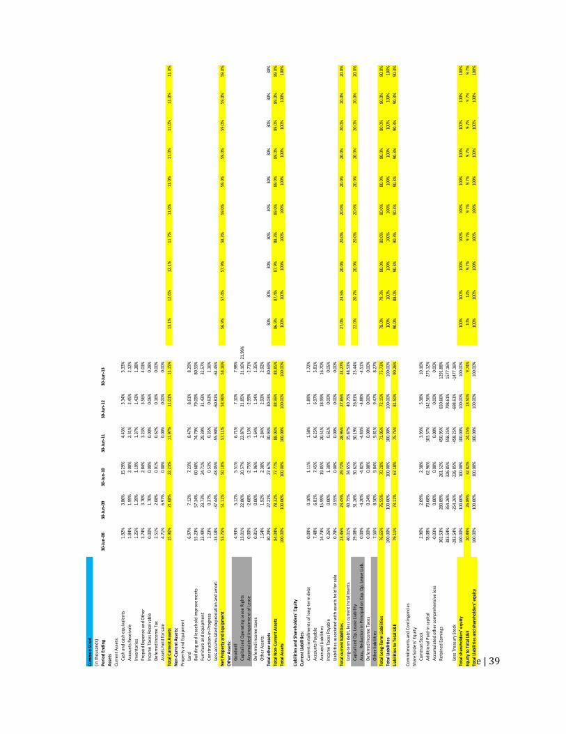
Page | 39
Com
mon
Siz
ed
(in
thou
sand
s)
Peri
od E
ndin
g 30
-Jun
-08
30-J
un-0
930
-Jun
-10
30-J
un-1
130
-Jun
-12
30-J
un-1
3
Ass
ets
Curr
ent A
sset
s:
Cash
and
cas
h eq
uiva
lent
s1.
92%
3.86
%15
.29%
4.43
%3.
34%
3.33
%
Acc
ount
s Re
ceiv
ale
1.84
%1.
99%
2.00
%2.
31%
2.45
%2.
12%
Inve
ntor
ies
1.25
%1.
39%
1.19
%1.
37%
1.43
%1.
38%
Prep
aid
Expe
nse
and
Oth
er3.
74%
3.70
%2.
84%
3.23
%3.
56%
4.03
%
Inco
me
Taxe
s Re
ceiv
able
0.00
%1.
70%
0.00
%0.
00%
0.06
%0.
28%
Def
erre
d In
com
e Ta
x2.
51%
2.08
%0.
91%
0.62
%0.
16%
0.00
%
Ass
ets
held
for s
ale
4.71
%6.
97%
0.00
%0.
00%
0.00
%0.
00%
Tota
l Cur
rent
Ass
ets
15.9
6%21
.68%
22.2
3%11
.97%
11.0
1%11
.15%
13.1
%12
.6%
12.1
%11
.7%
11.0
%11
.0%
11.0
%11
.0%
11.0
%11
.0%
Non
-Cur
rent
Ass
ets:
Prop
erty
and
Equ
ipm
ent
Land
6.
97%
7.12
%7.
23%
8.47
%8.
61%
8.29
%
Build
ing
and
leas
ehol
d im
prov
emen
ts55
.23%
57.3
4%60
.68%
74.7
9%79
.09%
80.5
9%
Furn
itur
e an
d eq
uipm
ent
23.4
9%23
.73%
24.7
1%29
.39%
31.4
3%32
.57%
Cons
truc
tion
-in-
Prog
ress
1.23
%0.
37%
0.53
%0.
35%
0.63
%1.
16%
Less
acc
umul
ated
dep
reci
atio
n an
d am
ort.
-33.
18%
-37.
44%
-43.
05%
-55.
90%
-60.
81%
-64.
45%
Net
Pro
pert
y an
d Eq
uipm
ent
53.7
5%51
.11%
50.1
0%57
.11%
58.9
6%58
.16%
56.9
%57
.4%
57.9
%58
.3%
59.0
%59
.0%
59.0
%59
.0%
59.0
%59
.0%
Oth
er A
sset
s:
Goo
dwill
4.93
%5.
12%
5.51
%6.
71%
7.10
%7.
98%
Capi
taliz
ed O
pera
ting
Lea
se R
ight
s23
.01%
22.8
6%20
.57%
22.8
7%21
.85%
21.1
6%21
.96%
Acc
umul
ated
Impa
irm
ent o
f Lea
se0.
00%
-2.6
8%-2
.75%
-3.1
3%-2
.99%
-2.7
1%
Def
erre
d in
com
e ta
xes
0.81
%0.
00%
1.96
%1.
64%
1.14
%1.
35%
Oth
er A
sset
s:1.
54%
1.92
%2.
38%
2.84
%2.
93%
2.92
%
Tota
l oth
er a
sset
s30
.29%
27.2
1%27
.67%
30.9
3%30
.03%
30.6
9%30
%30
%30
%30
%30
%30
%30
%30
%30
%30
%
Tota
l Non
-Cur
rent
Ass
ets
84.0
4%78
.32%
77.7
7%88
.03%
88.9
9%88
.85%
86.9
%87
.4%
87.9
%88
.3%
89.0
%89
.0%
89.0
%89
.0%
89.0
%89
.0%
Tota
l Ass
ets
100.
00%
100.
00%
100.
00%
100.
00%
100.
00%
100.
00%
100%
100%
100%
100%
100%
100%
100%
100%
100%
100%
Liab
iliti
es a
nd S
hare
hold
ers'
Equ
ity
Curr
ent L
iabi
litie
s:
Curr
ent i
nsta
llmen
ts o
f lon
g-te
rm d
ebt
0.09
%0.
10%
1.11
%1.
58%
1.89
%1.
72%
Acc
ount
s Pa
yabl
e7.
48%
6.81
%7.
45%
6.25
%6.
97%
5.81
%
Acc
rued
Lia
bilit
ies
14.7
3%15
.99%
19.8
5%20
.51%
18.9
9%16
.70%
Inco
me
Taxe
s Pa
yabl
e0.
26%
0.00
%1.
30%
0.61
%0.
00%
0.05
%
Liab
iliti
es a
ssoc
iate
d w
ith
asse
ts h
eld
for s
ale
0.78
%0.
55%
0.00
%0.
00%
0.00
%0.
00%
Tota
l cur
rent
liab
iliti
es23
.35%
23.4
5%29
.72%
28.9
5%27
.85%
24.2
7%27
.0%
23.5
%20
.0%
20.0
%20
.0%
20.0
%20
.0%
20.0
%20
.0%
20.0
%
Long
-ter
m d
ebt,
less
cur
rent
inst
allm
ents
40.0
1%40
.75%
34.6
5%35
.87%
40.7
5%48
.53%
Capi
taliz
ed O
p. L
ease
Lia
bilit
y29
.08%
31.2
6%30
.62%
30.1
9%26
.81%
23.4
4%22
.0%
20.7
%20
.0%
20.0
%20
.0%
20.0
%20
.0%
20.0
%20
.0%
20.0
%
Acc
u,. R
educ
tion
in P
rinc
ipal
on
Cap.
Op.
Lea
se L
iab.
0.
00%
-4.2
0%-4
.82%
-4.8
3%-4
.88%
-4.5
1%
Def
erre
d In
com
e Ta
xes
0.00
%0.
24%
0.00
%0.
00%
0.00
%0.
00%
Oth
er li
abili
ties
7.
56%
8.50
%9.
84%
9.81
%9.
47%
8.27
%
Tota
l Lon
g-Te
rm L
iabi
litie
s76
.65%
76.5
5%70
.28%
71.0
5%72
.15%
75.7
3%78
.0%
79.3
%80
.0%
80.0
%80
.0%
80.0
%80
.0%
80.0
%80
.0%
80.0
%
Tota
l Lia
bilit
ies
100.
00%
100.
00%
100.
00%
100.
00%
100.
00%
100.
00%
100%
100%
100%
100%
100%
100%
100%
100%
100%
100%
Liab
iliti
es to
Tot
al L
&E
79.1
1%73
.11%
67.1
8%75
.75%
81.5
0%90
.26%
90.0
%88
.0%
90.3
%90
.3%
90.3
%90
.3%
90.3
%90
.3%
90.3
%90
.3%
Com
mit
men
ts a
nd C
onti
ngen
cies
Shar
ehol
ders
' Equ
ity
Com
mon
Sto
ck2.
96%
2.69
%2.
38%
3.93
%5.
38%
10.1
6%
Add
itio
nal P
aid-
in c
apit
al
78.0
8%70
.68%
62.9
6%10
3.37
%14
2.56
%27
5.12
%
Acc
umul
ated
oth
er c
ompr
ehen
sive
loss
-0.0
3%0.
00%
0.00
%0.
00%
0.00
%0.
00%
Reta
ined
Ear
ning
s30
2.53
%28
0.89
%26
1.52
%45
0.95
%65
0.66
%12
91.8
8%
383.
54%
354.
26%
326.
85%
558.
25%
798.
61%
1577
.16%
Less
Tre
asur
y St
ock
-283
.54%
-254
.26%
-226
.85%
-458
.25%
-698
.61%
-147
7.16
%
Tota
l sha
reho
lder
s' e
quit
y10
0.00
%10
0.00
%10
0.00
%10
0.00
%10
0.00
%10
0.00
%10
0%10
0%10
0%10
0%10
0%10
0%10
0%10
0%10
0%10
0%
Equi
ty to
Tot
al L
&E
20.8
9%26
.89%
32.8
2%24
.25%
18.5
0%9.
74%
10%
12%
9.7%
9.7%
9.7%
9.7%
9.7%
9.7%
9.7%
9.7%
Tota
l Lia
bilit
ies
and
shar
ehol
ders
' equ
ity
100.
00%
100.
00%
100.
00%
100.
00%
100.
00%
100.
00%
100%
100%
100%
100%
100%
100%
100%
100%
100%
100%
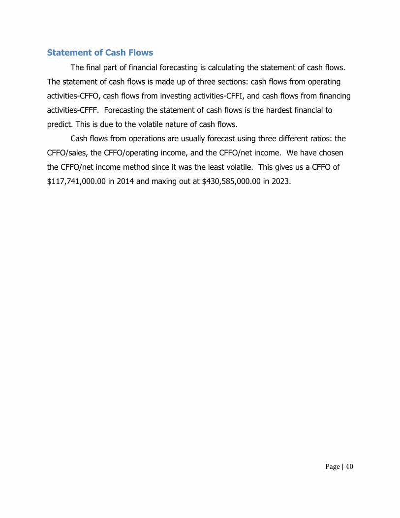
Page | 40
Statement of Cash Flows
The final part of financial forecasting is calculating the statement of cash flows.
The statement of cash flows is made up of three sections: cash flows from operating
activities-CFFO, cash flows from investing activities-CFFI, and cash flows from financing
activities-CFFF. Forecasting the statement of cash flows is the hardest financial to
predict. This is due to the volatile nature of cash flows.
Cash flows from operations are usually forecast using three different ratios: the
CFFO/sales, the CFFO/operating income, and the CFFO/net income. We have chosen
the CFFO/net income method since it was the least volatile. This gives us a CFFO of
$117,741,000.00 in 2014 and maxing out at $430,585,000.00 in 2023.
Page | 41
As-
Stat
ed
Cas
hfl
ow
Sta
tem
en
t
(in
th
ou
san
dth
s)
Pe
rio
d E
nd
ing
30-J
un
-08
30-J
un
-09
30-J
un
-10
30-J
un
-11
30-J
un
-12
30-J
un
-13
2014
2015
2016
2017
2018
2019
2020
2021
2022
2023
Ne
t In
com
e51
,722
79
,166
13
7,70
4
14
1,06
0
15
1,23
2
16
3,35
9
Acc
rual
Ad
just
me
nts
to
co
mp
ute
CFF
O27
4,98
7
154,
841
15
9,69
8
11
8,92
8
15
2,20
6
12
7,32
9
T
ota
l Cas
h F
low
Fro
m O
pe
rati
ng
Act
ivit
ies
326,
709
23
4,00
7
297,
402
259,
988
303,
438
290,
688
Op
Me
tho
d11
0,19
4
119,
984
140,
748
168,
897
214,
077
246,
189
283,
117
32
5,58
4
37
4,42
2
43
0,58
5
NI M
eth
od
117,
741
12
8,20
3
14
6,39
5
17
2,94
6
21
4,07
7
24
6,18
9
28
3,11
7
325,
584
374,
422
430,
585
Ave
rage
Sale
s/C
FFO
10.0
815
.91
14.6
419
.26
18.9
822
.79
20.3
4
OP
Inc/
CFF
O1.
141.
911.
902.
502.
472.
962.
64
Ne
t In
c/C
FFO
0.67
1.10
1.07
1.41
1.39
1.66
1.49
Inve
stin
g A
ctiv
itie
s C
ash
flo
ws
C
apit
al E
xpe
nd
itu
res
-259
356
-881
52-6
0879
-703
61-1
2834
6-1
5615
3
In
vest
me
nts
-871
1-4
612
0-2
896
-317
00
O
the
r C
ash
flo
ws
fro
m In
vest
ing
Act
ivit
ies
9334
586
553
5635
286
9681
1218
309
T
ota
l Cas
h F
low
s fr
om
Inve
stin
g A
ctiv
itie
s-1
7472
2-6
211
-452
7-6
4,56
1-1
23,4
04-1
37,8
44
Fin
anci
ng
Act
ivit
ies
Cas
h F
low
s
D
ivid
en
ds
Pai
d-4
2914
-453
55-3
4448
-531
85-5
0,08
1-5
6343
Sa
le o
f St
ock
5277
4650
2396
3305
743
416
4119
0
P
urc
has
e o
f St
ock
-240
784
-373
9-2
2868
-422
099
-287
291
-333
384
N
et
Bo
rro
win
gs-3
2358
6-1
6075
70
040
000
-400
00
O
the
r C
ash
flo
ws
fro
m F
inan
cin
g A
ctiv
itie
s39
8555
-191
84-1
9451
8-1
5,83
651
,037
235,
957
T
ota
l Cas
h F
low
s Fr
om
Fin
anci
ng
Act
ivit
ies
-203
452
-224
385
-249
438
-458
,063
-202
,919
-152
,580
Ne
t C
han
g in
Cas
h &
Cas
h E
qu
ival
en
ts-3
0,10
939
,442
250,
468
-262
,636
-22,
885
264
Cas
h &
Cas
h E
qu
ival
en
ts B
egi
nn
ing
Bal
ance
8482
354
,714
94,1
5634
4,62
481
,988
59,1
03
Cas
h &
Cas
h E
qu
ival
en
ts E
nd
ing
Bal
ance
54,7
1494
,156
344,
624
81,9
8859
,103
59,3
67
Co
mm
on
Siz
e C
ash
flo
w S
tate
me
nt
(in
th
ou
san
dth
s)
Pe
rio
d E
nd
ing
30-J
un
-08
30-J
un
-09
30-J
un
-10
30-J
un
-11
30-J
un
-12
30-J
un
-13
Ne
t In
com
e15
.83%
33.8
3%46
.30%
54.2
6%49
.84%
56.2
0%
Acc
rual
Ad
just
me
nts
to
co
mp
ute
CFF
O84
.17%
66.1
7%53
.70%
45.7
4%50
.16%
43.8
0%
T
ota
l Cas
h F
low
Fro
m O
pe
rati
ng
Act
ivit
ies
100.
00%
100.
00%
100.
00%
100.
00%
100.
00%
100.
00%
Inve
stin
g A
ctiv
itie
s C
ash
flo
ws
C
apit
al E
xpe
nd
itu
res
-79.
38%
-37.
67%
-20.
47%
-27.
06%
-42.
30%
-53.
72%
In
vest
me
nts
-2.6
7%-1
.97%
0.00
%-1
.11%
-1.0
4%0.
00%
O
the
r C
ash
flo
ws
fro
m In
vest
ing
Act
ivit
ies
28.5
7%36
.99%
18.9
5%3.
34%
2.67
%6.
30%
T
ota
l Cas
h F
low
s fr
om
Inve
stin
g A
ctiv
itie
s-5
3.48
%-2
.65%
-1.5
2%-2
4.83
%-4
0.67
%-4
7.42
%
Fin
anci
ng
Act
ivit
ies
Cas
h F
low
s
D
ivid
en
ds
Pai
d-1
3.14
%-1
9.38
%-1
1.58
%-2
0.46
%-1
6.50
%-1
9.38
%
Sa
le o
f St
ock
1.62
%1.
99%
0.81
%12
.71%
14.3
1%14
.17%
P
urc
has
e o
f St
ock
-73.
70%
-1.6
0%-7
.69%
-162
.35%
-94.
68%
-114
.69%
N
et
Bo
rro
win
gs-9
9.04
%-6
8.70
%0.
00%
0.00
%13
.18%
-13.
76%
O
the
r C
ash
flo
ws
fro
m F
inan
cin
g A
ctiv
itie
s12
1.99
%-8
.20%
-65.
41%
-6.0
9%16
.82%
81.1
7%
T
ota
l Cas
h F
low
s Fr
om
Fin
anci
ng
Act
ivit
ies
-62.
27%
-95.
89%
-83.
87%
-176
.19%
-66.
87%
-52.
49%
Ne
t C
han
g in
Cas
h &
Cas
h E
qu
ival
en
ts-9
.22%
16.8
6%84
.22%
-101
.02%
-7.5
4%0.
09%
Cas
h &
Cas
h E
qu
ival
en
ts B
egi
nn
ing
Bal
ance
25.9
6%23
.38%
31.6
6%13
2.55
%27
.02%
20.3
3%
Cas
h &
Cas
h E
qu
ival
en
ts E
nd
ing
Bal
ance
16.7
5%40
.24%
115.
88%
31.5
4%19
.48%
20.4
2%
Page | 42
Restated Financial Statements
After restating the financial statements of Brinker International, we have found
there to be no significant changes to the income statement or balance sheet. Both
goodwill and capitalization of operating leases were immaterial amounts.
Cost of Capital Estimation
In order to determine a relative value of a firm, the discount rate for debt and
equity holders must be calculated to discount the firm’s financials. The weighted
average cost of capital (WACC) is the discount rate that will be used. The WACC
illustrates two ways companies can obtain funding from debt and equity. To calculate
the WACC, both the cost of debt and the cost of equity need to be estimated. In the
following section(s) Brinker’s cost of debt and cost of equity will be estimated, and then
used to calculate the company’s WACC. If in the event that the cost of capital is
relatively high or low, the firm is relatively understated or overstated respectfully.
Cost of Debt
The cost of debt refers to the overall effective interest rate a company is paying
on their debt financing. Generally, the higher the cost of debt results in a higher risk
associated with the firm. Due to the fact that debt holders have a superior claim on
assets and a lower associated risk, the cost of debt is typically lower than the cost of
equity.
To calculate the weighted average cost of debt for Brinker, all current and non-
current interest bearing liabilities are taken into account. Non-interest bearing debts
are considered to be non-financial liabilities, as a result we adjusted the balance sheet
to reflect the removal of non-interest bearing accounts from both the left- and right-
hand side of the balance sheet. Next, we had to find the associated interest rates for
the current and non-current liabilities.
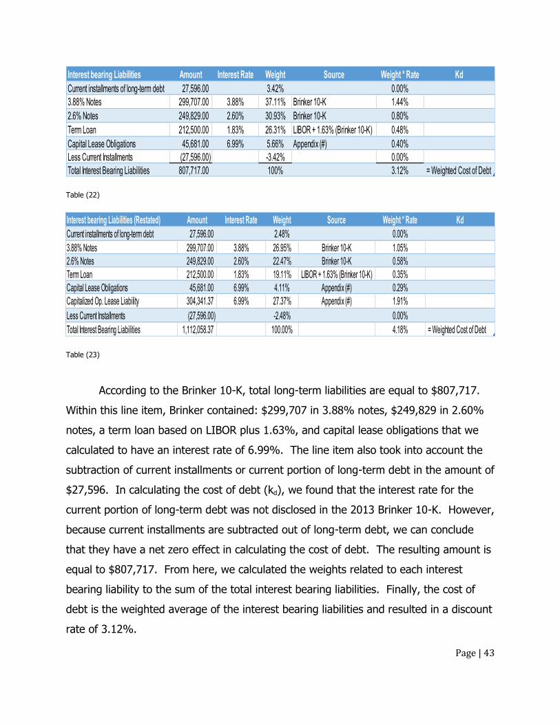
Page | 43
Table (22)
Table (23)
According to the Brinker 10-K, total long-term liabilities are equal to $807,717.
Within this line item, Brinker contained: $299,707 in 3.88% notes, $249,829 in 2.60%
notes, a term loan based on LIBOR plus 1.63%, and capital lease obligations that we
calculated to have an interest rate of 6.99%. The line item also took into account the
subtraction of current installments or current portion of long-term debt in the amount of
$27,596. In calculating the cost of debt (kd), we found that the interest rate for the
current portion of long-term debt was not disclosed in the 2013 Brinker 10-K. However,
because current installments are subtracted out of long-term debt, we can conclude
that they have a net zero effect in calculating the cost of debt. The resulting amount is
equal to $807,717. From here, we calculated the weights related to each interest
bearing liability to the sum of the total interest bearing liabilities. Finally, the cost of
debt is the weighted average of the interest bearing liabilities and resulted in a discount
rate of 3.12%.
Interest bearing Liabilities Amount Interest Rate Weight Source Weight * Rate Kd
Current installments of long-term debt 27,596.00 3.42% 0.00%
3.88% Notes 299,707.00 3.88% 37.11% Brinker 10-K 1.44%
2.6% Notes 249,829.00 2.60% 30.93% Brinker 10-K 0.80%
Term Loan 212,500.00 1.83% 26.31% LIBOR + 1.63% (Brinker 10-K) 0.48%
Capital Lease Obligations 45,681.00 6.99% 5.66% Appendix (#) 0.40%
Less Current Installments (27,596.00) -3.42% 0.00%
Total Interest Bearing Liabilities 807,717.00 100% 3.12% = Weighted Cost of Debt
Interest bearing Liabilities (Restated) Amount Interest Rate Weight Source Weight * Rate Kd
Current installments of long-term debt 27,596.00 2.48% 0.00%
3.88% Notes 299,707.00 3.88% 26.95% Brinker 10-K 1.05%
2.6% Notes 249,829.00 2.60% 22.47% Brinker 10-K 0.58%
Term Loan 212,500.00 1.83% 19.11% LIBOR + 1.63% (Brinker 10-K) 0.35%
Capital Lease Obligations 45,681.00 6.99% 4.11% Appendix (#) 0.29%
Capitalized Op. Lease Liability 304,341.37 6.99% 27.37% Appendix (#) 1.91%
Less Current Installments (27,596.00) -2.48% 0.00%
Total Interest Bearing Liabilities 1,112,058.37 100.00% 4.18% = Weighted Cost of Debt
Page | 44
When looking at the restated balance sheet for 2013, it is evident that the
capitalization of operating leases does not have a large impact of cost of debt. The
increase in capitalized operating leases increased cost of debt from 3.12% to 4.18% by
changing the relative weights of the other interest bearing debt. This means that
Brinker is expected to pay on average 4.18% in interest for every dollar of debt instead
of 3.12%.
Cost of Equity
The cost of equity (ke) can also be stated as the return on equity that
shareholders require. For a firm, the cost of equity represents the return that the
market warrants for the risk taken in an ownership stake of a company. The cost of
equity is computed using the Capital Asset Pricing Model (CAPM). The CAPM formula is:
( )
This formula takes into account the risk free rate (Rf), systematic risk (beta), the
market risk premium (Rm-Rf), and a size adjusted beta (Bsize). To find the risk free rate,
we found the yields for 3-month, 1-year, 2-year, 7-year, and 10-year treasury bonds via
the St. Louis Federal Reserve website. However, because these yields are provided in
an annual basis, we had to convert this annual rate to a monthly rate. For this analysis,
the most recent 10-year treasury rate was used, and was found to be 2.71%.
The market return is the rate of return that has been realized in the overall
market. For this analysis, the market return was taken from the historical returns of the
S&P 500. The market risk premium is the additional benefit that an investor expects to
earn when taking on the added risk of the market. To calculate the market risk
premium, we subtracted the risk free rate from the historical S&P 500 returns.
However, because of recent governmental influence over interest rates, the market risk
premium is understated. For this reason, we use an 8% market risk premium as a
realistic estimate based on the historical long-run market risk premiums.
Beta, also known as the beta coefficient, is a measure of systematic (market)
risk. In order to estimate beta, we conducted multiple regressions utilizing the
Page | 45
historical company returns and the market risk premiums associated with the relative
treasury yields. Appendix (1) provides the regression table information for the year
2013. From the regression tables we are able to obtain a beta of 1.40 with a lower and
upper bound for 72 months of 0.89 and 1.92 for the 10-year regression with a 95%
confidence level. According to YahooFinance.com, Brinker has a beta of 0.69. This
beta is not within the realm of our 95% confidence level, but it shows that the analysts
believe that Brinker has a systematic risk at the very low end of the spectrum. The
regression tables also show the adjusted R2, which is the percentage of systematic risk
associated with a company. The following table shows the regression table results:
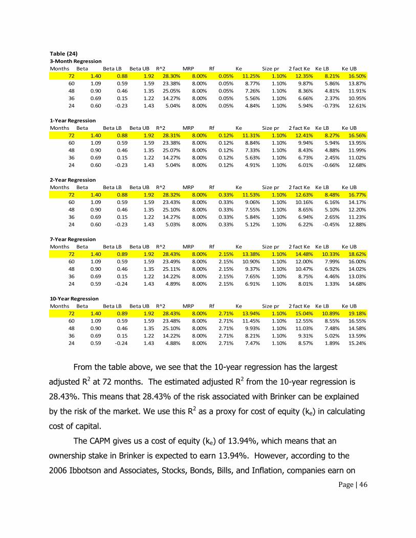
Page | 46
From the table above, we see that the 10-year regression has the largest
adjusted R2 at 72 months. The estimated adjusted R2 from the 10-year regression is
28.43%. This means that 28.43% of the risk associated with Brinker can be explained
by the risk of the market. We use this R2 as a proxy for cost of equity (ke) in calculating
cost of capital.
The CAPM gives us a cost of equity (ke) of 13.94%, which means that an
ownership stake in Brinker is expected to earn 13.94%. However, according to the
2006 Ibbotson and Associates, Stocks, Bonds, Bills, and Inflation, companies earn on
Table (24)3-Month Regression
Months Beta Beta LB Beta UB R^2 MRP Rf Ke Size pr 2 fact Ke Ke LB Ke UB
72 1.40 0.88 1.92 28.30% 8.00% 0.05% 11.25% 1.10% 12.35% 8.21% 16.50%
60 1.09 0.59 1.59 23.38% 8.00% 0.05% 8.77% 1.10% 9.87% 5.86% 13.87%
48 0.90 0.46 1.35 25.05% 8.00% 0.05% 7.26% 1.10% 8.36% 4.81% 11.91%
36 0.69 0.15 1.22 14.27% 8.00% 0.05% 5.56% 1.10% 6.66% 2.37% 10.95%
24 0.60 -0.23 1.43 5.04% 8.00% 0.05% 4.84% 1.10% 5.94% -0.73% 12.61%
1-Year Regression
Months Beta Beta LB Beta UB R^2 MRP Rf Ke Size pr 2 fact Ke Ke LB Ke UB
72 1.40 0.88 1.92 28.31% 8.00% 0.12% 11.31% 1.10% 12.41% 8.27% 16.56%
60 1.09 0.59 1.59 23.38% 8.00% 0.12% 8.84% 1.10% 9.94% 5.94% 13.95%
48 0.90 0.46 1.35 25.07% 8.00% 0.12% 7.33% 1.10% 8.43% 4.88% 11.99%
36 0.69 0.15 1.22 14.27% 8.00% 0.12% 5.63% 1.10% 6.73% 2.45% 11.02%
24 0.60 -0.23 1.43 5.04% 8.00% 0.12% 4.91% 1.10% 6.01% -0.66% 12.68%
2-Year Regression
Months Beta Beta LB Beta UB R^2 MRP Rf Ke Size pr 2 fact Ke Ke LB Ke UB
72 1.40 0.88 1.92 28.32% 8.00% 0.33% 11.53% 1.10% 12.63% 8.48% 16.77%
60 1.09 0.59 1.59 23.43% 8.00% 0.33% 9.06% 1.10% 10.16% 6.16% 14.17%
48 0.90 0.46 1.35 25.10% 8.00% 0.33% 7.55% 1.10% 8.65% 5.10% 12.20%
36 0.69 0.15 1.22 14.27% 8.00% 0.33% 5.84% 1.10% 6.94% 2.65% 11.23%
24 0.60 -0.23 1.43 5.03% 8.00% 0.33% 5.12% 1.10% 6.22% -0.45% 12.88%
7-Year Regression
Months Beta Beta LB Beta UB R^2 MRP Rf Ke Size pr 2 fact Ke Ke LB Ke UB
72 1.40 0.89 1.92 28.43% 8.00% 2.15% 13.38% 1.10% 14.48% 10.33% 18.62%
60 1.09 0.59 1.59 23.49% 8.00% 2.15% 10.90% 1.10% 12.00% 7.99% 16.00%
48 0.90 0.46 1.35 25.11% 8.00% 2.15% 9.37% 1.10% 10.47% 6.92% 14.02%
36 0.69 0.15 1.22 14.22% 8.00% 2.15% 7.65% 1.10% 8.75% 4.46% 13.03%
24 0.59 -0.24 1.43 4.89% 8.00% 2.15% 6.91% 1.10% 8.01% 1.33% 14.68%
10-Year Regression
Months Beta Beta LB Beta UB R^2 MRP Rf Ke Size pr 2 fact Ke Ke LB Ke UB
72 1.40 0.89 1.92 28.43% 8.00% 2.71% 13.94% 1.10% 15.04% 10.89% 19.18%
60 1.09 0.59 1.59 23.48% 8.00% 2.71% 11.45% 1.10% 12.55% 8.55% 16.55%
48 0.90 0.46 1.35 25.10% 8.00% 2.71% 9.93% 1.10% 11.03% 7.48% 14.58%
36 0.69 0.15 1.22 14.22% 8.00% 2.71% 8.21% 1.10% 9.31% 5.02% 13.59%
24 0.59 -0.24 1.43 4.88% 8.00% 2.71% 7.47% 1.10% 8.57% 1.89% 15.24%
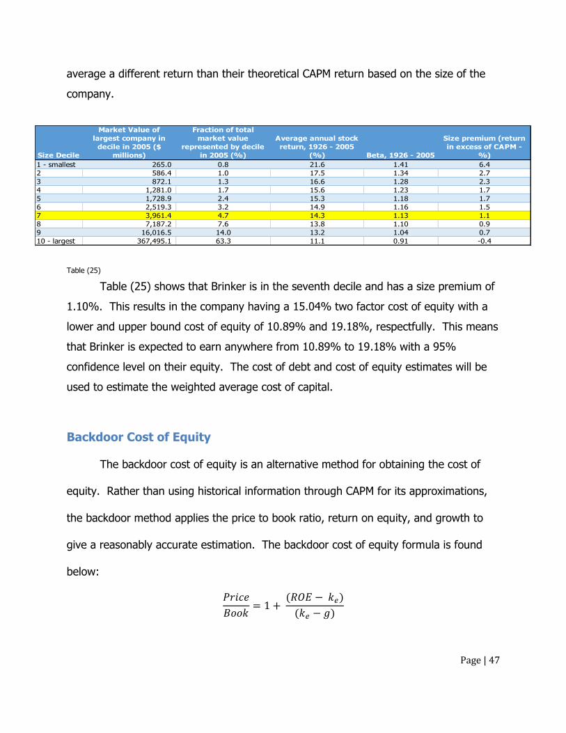
Page | 47
average a different return than their theoretical CAPM return based on the size of the
company.
Table (25)
Table (25) shows that Brinker is in the seventh decile and has a size premium of
1.10%. This results in the company having a 15.04% two factor cost of equity with a
lower and upper bound cost of equity of 10.89% and 19.18%, respectfully. This means
that Brinker is expected to earn anywhere from 10.89% to 19.18% with a 95%
confidence level on their equity. The cost of debt and cost of equity estimates will be
used to estimate the weighted average cost of capital.
Backdoor Cost of Equity The backdoor cost of equity is an alternative method for obtaining the cost of
equity. Rather than using historical information through CAPM for its approximations,
the backdoor method applies the price to book ratio, return on equity, and growth to
give a reasonably accurate estimation. The backdoor cost of equity formula is found
below:
Size Decile
Market Value of
largest company in
decile in 2005 ($
millions)
Fraction of total
market value
represented by decile
in 2005 (%)
Average annual stock
return, 1926 - 2005
(%) Beta, 1926 - 2005
Size premium (return
in excess of CAPM -
%)
1 - smallest 265.0 0.8 21.6 1.41 6.4
2 586.4 1.0 17.5 1.34 2.7
3 872.1 1.3 16.6 1.28 2.3
4 1,281.0 1.7 15.6 1.23 1.7
5 1,728.9 2.4 15.3 1.18 1.7
6 2,519.3 3.2 14.9 1.16 1.5
7 3,961.4 4.7 14.3 1.13 1.1
8 7,187.2 7.6 13.8 1.10 0.9
9 16,016.5 14.0 13.2 1.04 0.7
10 - largest 367,495.1 63.3 11.1 0.91 -0.4
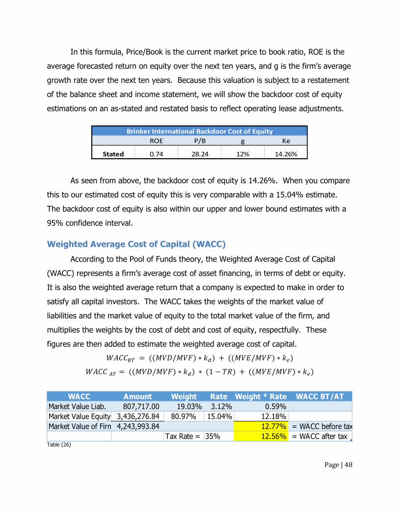
Page | 48
In this formula, Price/Book is the current market price to book ratio, ROE is the
average forecasted return on equity over the next ten years, and g is the firm’s average
growth rate over the next ten years. Because this valuation is subject to a restatement
of the balance sheet and income statement, we will show the backdoor cost of equity
estimations on an as-stated and restated basis to reflect operating lease adjustments.
As seen from above, the backdoor cost of equity is 14.26%. When you compare
this to our estimated cost of equity this is very comparable with a 15.04% estimate.
The backdoor cost of equity is also within our upper and lower bound estimates with a
95% confidence interval.
Weighted Average Cost of Capital (WACC)
According to the Pool of Funds theory, the Weighted Average Cost of Capital
(WACC) represents a firm’s average cost of asset financing, in terms of debt or equity.
It is also the weighted average return that a company is expected to make in order to
satisfy all capital investors. The WACC takes the weights of the market value of
liabilities and the market value of equity to the total market value of the firm, and
multiplies the weights by the cost of debt and cost of equity, respectfully. These
figures are then added to estimate the weighted average cost of capital.
Table (26)
WACC Amount Weight Rate Weight * Rate WACC BT/AT
Market Value Liab. 807,717.00 19.03% 3.12% 0.59%
Market Value Equity 3,436,276.84 80.97% 15.04% 12.18%
Market Value of Firm 4,243,993.84 12.77% = WACC before tax
Tax Rate = 35% 12.56% = WACC after tax
ROE P/B g Ke
Stated 0.74 28.24 12% 14.26%
Brinker International Backdoor Cost of Equity
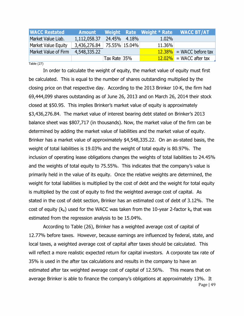
Page | 49
Table (27)
In order to calculate the weight of equity, the market value of equity must first
be calculated. This is equal to the number of shares outstanding multiplied by the
closing price on that respective day. According to the 2013 Brinker 10-K, the firm had
69,444,099 shares outstanding as of June 26, 2013 and on March 26, 2014 their stock
closed at $50.95. This implies Brinker’s market value of equity is approximately
$3,436,276.84. The market value of interest bearing debt stated on Brinker’s 2013
balance sheet was $807,717 (in thousands). Now, the market value of the firm can be
determined by adding the market value of liabilities and the market value of equity.
Brinker has a market value of approximately $4,548,335.22. On an as-stated basis, the
weight of total liabilities is 19.03% and the weight of total equity is 80.97%. The
inclusion of operating lease obligations changes the weights of total liabilities to 24.45%
and the weights of total equity to 75.55%. This indicates that the company’s value is
primarily held in the value of its equity. Once the relative weights are determined, the
weight for total liabilities is multiplied by the cost of debt and the weight for total equity
is multiplied by the cost of equity to find the weighted average cost of capital. As
stated in the cost of debt section, Brinker has an estimated cost of debt of 3.12%. The
cost of equity (ke) used for the WACC was taken from the 10-year 2-factor ke that was
estimated from the regression analysis to be 15.04%.
According to Table (26), Brinker has a weighted average cost of capital of
12.77% before taxes. However, because earnings are influenced by federal, state, and
local taxes, a weighted average cost of capital after taxes should be calculated. This
will reflect a more realistic expected return for capital investors. A corporate tax rate of
35% is used in the after tax calculations and results in the company to have an
estimated after tax weighted average cost of capital of 12.56%. This means that on
average Brinker is able to finance the company’s obligations at approximately 13%. It
WACC Restated Amount Weight Rate Weight * Rate WACC BT/AT
Market Value Liab. 1,112,058.37 24.45% 4.18% 1.02%
Market Value Equity 3,436,276.84 75.55% 15.04% 11.36%
Market Value of Firm 4,548,335.22 12.38% = WACC before tax
Tax Rate 35% 12.02% = WACC after tax
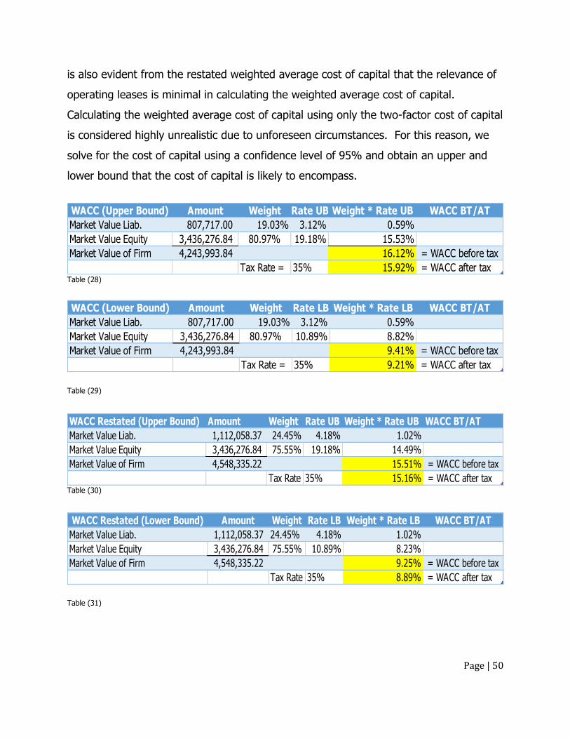
Page | 50
is also evident from the restated weighted average cost of capital that the relevance of
operating leases is minimal in calculating the weighted average cost of capital.
Calculating the weighted average cost of capital using only the two-factor cost of capital
is considered highly unrealistic due to unforeseen circumstances. For this reason, we
solve for the cost of capital using a confidence level of 95% and obtain an upper and
lower bound that the cost of capital is likely to encompass.
Table (28)
Table (29)
Table (30)
Table (31)
WACC (Lower Bound) Amount Weight Rate LB Weight * Rate LB WACC BT/AT
Market Value Liab. 807,717.00 19.03% 3.12% 0.59%
Market Value Equity 3,436,276.84 80.97% 10.89% 8.82%
Market Value of Firm 4,243,993.84 9.41% = WACC before tax
Tax Rate = 35% 9.21% = WACC after tax
WACC (Upper Bound) Amount Weight Rate UB Weight * Rate UB WACC BT/AT
Market Value Liab. 807,717.00 19.03% 3.12% 0.59%
Market Value Equity 3,436,276.84 80.97% 19.18% 15.53%
Market Value of Firm 4,243,993.84 16.12% = WACC before tax
Tax Rate = 35% 15.92% = WACC after tax
WACC Restated (Upper Bound) Amount Weight Rate UB Weight * Rate UB WACC BT/AT
Market Value Liab. 1,112,058.37 24.45% 4.18% 1.02%
Market Value Equity 3,436,276.84 75.55% 19.18% 14.49%
Market Value of Firm 4,548,335.22 15.51% = WACC before tax
Tax Rate 35% 15.16% = WACC after tax
WACC Restated (Lower Bound) Amount Weight Rate LB Weight * Rate LB WACC BT/AT
Market Value Liab. 1,112,058.37 24.45% 4.18% 1.02%
Market Value Equity 3,436,276.84 75.55% 10.89% 8.23%
Market Value of Firm 4,548,335.22 9.25% = WACC before tax
Tax Rate 35% 8.89% = WACC after tax
Page | 51
By utilizing the 95% confidence level of the cost of equity, we are able to
estimate a range of the upper and lower bounds for the weighted average cost of
capital. We can then assume that the true weighted average cost of capital for Brinker
lies within this range. The above charts show a range of 9.21% to 15.92% for the
after-tax weight average cost of capital on an as stated basis. On a restated basis, this
range falls to 8.89% to 15.16%. From this information we can conclude that the
restatement has a marginal effect on the cost of capital. As a result of this analysis, the
most appropriate discount to be used lies within our upper and lower bound restated
after-tax cost of capital.

Page | 52
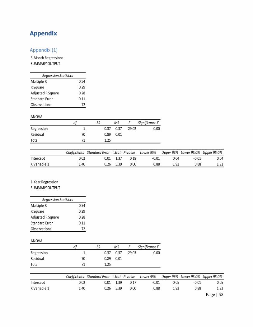
Page | 53
Appendix
Appendix (1)
3-Month Regressions
SUMMARY OUTPUT
Regression Statistics
Multiple R 0.54
R Square 0.29
Adjusted R Square 0.28
Standard Error 0.11
Observations 72
ANOVA
df SS MS F Significance F
Regression 1 0.37 0.37 29.02 0.00
Residual 70 0.89 0.01
Total 71 1.25
Coefficients Standard Error t Stat P-value Lower 95% Upper 95% Lower 95.0% Upper 95.0%
Intercept 0.02 0.01 1.37 0.18 -0.01 0.04 -0.01 0.04
X Variable 1 1.40 0.26 5.39 0.00 0.88 1.92 0.88 1.92
1-Year Regression
SUMMARY OUTPUT
Regression Statistics
Multiple R 0.54
R Square 0.29
Adjusted R Square 0.28
Standard Error 0.11
Observations 72
ANOVA
df SS MS F Significance F
Regression 1 0.37 0.37 29.03 0.00
Residual 70 0.89 0.01
Total 71 1.25
Coefficients Standard Error t Stat P-value Lower 95% Upper 95% Lower 95.0% Upper 95.0%
Intercept 0.02 0.01 1.39 0.17 -0.01 0.05 -0.01 0.05
X Variable 1 1.40 0.26 5.39 0.00 0.88 1.92 0.88 1.92
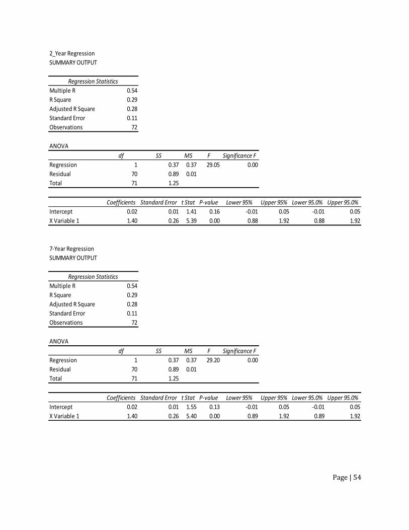
Page | 54
2_Year Regression
SUMMARY OUTPUT
Regression Statistics
Multiple R 0.54
R Square 0.29
Adjusted R Square 0.28
Standard Error 0.11
Observations 72
ANOVA
df SS MS F Significance F
Regression 1 0.37 0.37 29.05 0.00
Residual 70 0.89 0.01
Total 71 1.25
Coefficients Standard Error t Stat P-value Lower 95% Upper 95% Lower 95.0% Upper 95.0%
Intercept 0.02 0.01 1.41 0.16 -0.01 0.05 -0.01 0.05
X Variable 1 1.40 0.26 5.39 0.00 0.88 1.92 0.88 1.92
7-Year Regression
SUMMARY OUTPUT
Regression Statistics
Multiple R 0.54
R Square 0.29
Adjusted R Square 0.28
Standard Error 0.11
Observations 72
ANOVA
df SS MS F Significance F
Regression 1 0.37 0.37 29.20 0.00
Residual 70 0.89 0.01
Total 71 1.25
Coefficients Standard Error t Stat P-value Lower 95% Upper 95% Lower 95.0% Upper 95.0%
Intercept 0.02 0.01 1.55 0.13 -0.01 0.05 -0.01 0.05
X Variable 1 1.40 0.26 5.40 0.00 0.89 1.92 0.89 1.92
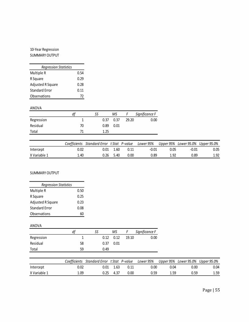
Page | 55
10-Year Regression
SUMMARY OUTPUT
Regression Statistics
Multiple R 0.54
R Square 0.29
Adjusted R Square 0.28
Standard Error 0.11
Observations 72
ANOVA
df SS MS F Significance F
Regression 1 0.37 0.37 29.20 0.00
Residual 70 0.89 0.01
Total 71 1.25
Coefficients Standard Error t Stat P-value Lower 95% Upper 95% Lower 95.0% Upper 95.0%
Intercept 0.02 0.01 1.60 0.11 -0.01 0.05 -0.01 0.05
X Variable 1 1.40 0.26 5.40 0.00 0.89 1.92 0.89 1.92
SUMMARY OUTPUT
Regression Statistics
Multiple R 0.50
R Square 0.25
Adjusted R Square 0.23
Standard Error 0.08
Observations 60
ANOVA
df SS MS F Significance F
Regression 1 0.12 0.12 19.10 0.00
Residual 58 0.37 0.01
Total 59 0.49
Coefficients Standard Error t Stat P-value Lower 95% Upper 95% Lower 95.0% Upper 95.0%
Intercept 0.02 0.01 1.63 0.11 0.00 0.04 0.00 0.04
X Variable 1 1.09 0.25 4.37 0.00 0.59 1.59 0.59 1.59
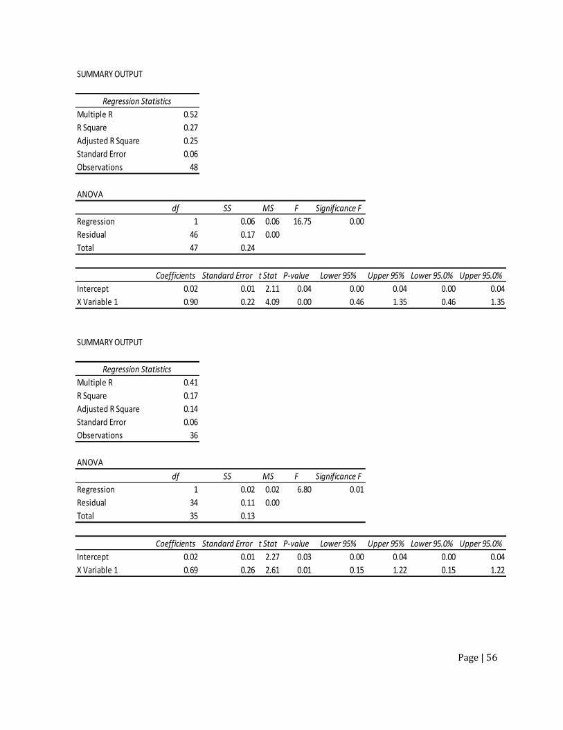
Page | 56
SUMMARY OUTPUT
Regression Statistics
Multiple R 0.52
R Square 0.27
Adjusted R Square 0.25
Standard Error 0.06
Observations 48
ANOVA
df SS MS F Significance F
Regression 1 0.06 0.06 16.75 0.00
Residual 46 0.17 0.00
Total 47 0.24
Coefficients Standard Error t Stat P-value Lower 95% Upper 95% Lower 95.0% Upper 95.0%
Intercept 0.02 0.01 2.11 0.04 0.00 0.04 0.00 0.04
X Variable 1 0.90 0.22 4.09 0.00 0.46 1.35 0.46 1.35
SUMMARY OUTPUT
Regression Statistics
Multiple R 0.41
R Square 0.17
Adjusted R Square 0.14
Standard Error 0.06
Observations 36
ANOVA
df SS MS F Significance F
Regression 1 0.02 0.02 6.80 0.01
Residual 34 0.11 0.00
Total 35 0.13
Coefficients Standard Error t Stat P-value Lower 95% Upper 95% Lower 95.0% Upper 95.0%
Intercept 0.02 0.01 2.27 0.03 0.00 0.04 0.00 0.04
X Variable 1 0.69 0.26 2.61 0.01 0.15 1.22 0.15 1.22
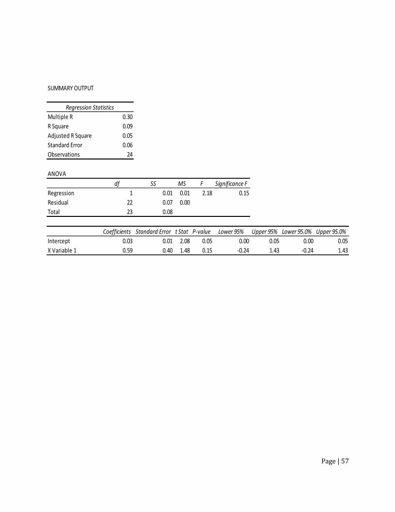
Page | 57
SUMMARY OUTPUT
Regression Statistics
Multiple R 0.30
R Square 0.09
Adjusted R Square 0.05
Standard Error 0.06
Observations 24
ANOVA
df SS MS F Significance F
Regression 1 0.01 0.01 2.18 0.15
Residual 22 0.07 0.00
Total 23 0.08
Coefficients Standard Error t Stat P-value Lower 95% Upper 95% Lower 95.0% Upper 95.0%
Intercept 0.03 0.01 2.08 0.05 0.00 0.05 0.00 0.05
X Variable 1 0.59 0.40 1.48 0.15 -0.24 1.43 -0.24 1.43

Page | 58


![[Draft] International Financial Reporting Standard X](https://img.pdfslide.net/doc/110x75/55491481b4c90558458c12fa/draft-international-financial-reporting-standard-x.jpg)