Embed Size (px)
Citation preview
1
Financial Contagion from the US Structured
Finance Market: Evidence from International
Markets and Asset Pricing Perspectives
by
Woon Sau Leung
A Thesis Submitted in Partial Fulfilment of the Requirements for the
Degree of Doctor of Philosophy of Cardiff University
Department of Accounting and Finance of Cardiff Business School,
Cardiff University
April 2014

2
DECLARATION
This work has not previously been accepted in substance for any degree and is not
concurrently submitted in candidature for any degree.
Signed …………………………………………………………. (Woon Sau Leung)
Date …………………………
STATEMENT 1
This thesis is being submitted in partial fulfilment of the requirements for the degree of
Doctor of Philosophy of Cardiff University.
Signed …………………………………………………………. (Woon Sau Leung)
Date …………………………
STATEMENT 2
This thesis is the result of my own independent work/investigation, except where
otherwise stated. Other sources are acknowledged by footnotes giving explicit references.
Signed …………………………………………………………. (Woon Sau Leung)
Date …………………………
STATEMENT 3
I hereby give consent for my thesis, if accepted, to be available for photocopying and for
inter-library loan, and for the title and summary to be made available to outside
organisations.
Signed …………………………………………………………. (Woon Sau Leung)
Date …………………………
Financial Contagion From The US Structured Finance Market: Evidence From
International Markets and Asset Pricing Perspectives
by
Woon Sau Leung
Submitted to the Department of Accounting and Financeon April 3, 2014, in partial fulfillment of the
requirements for the degree ofDoctor of Philosophy
Abstract
Given the growing importance of securitisation to financial stability, it is surprising that empiricalstudies on the role of the US structured finance market in the recent crisis have been relativelysparse. To fill this gap, this thesis studies the US structured finance market (tracked by the ABXindices) and addresses various important research questions specific to the recent 2007 to 2009financial crisis. First, I contribute to the contagion literature by extending Longstaff’s (2010)investigation to an international market perspective. Evidence of contagion from the ABX indicesto the G5 international equity and government bond markets via the funding illiquidity and creditrisk channels during the subprime crisis is documented. Second, I formulate a multifactor modelwith crisis interaction effects and document significant increases in the ABX AAA factor loadingsduring the subprime crisis, which is consistent with contagion. My cross-sectional pricing testsshow that the ABX AAA factor significantly explains the cross-section of expected returns duringthe subprime crisis; that is, the impact of contagion on the US equity market was reasonablysystematic. I compute a simple statistic that gauges the degree of the stocks’ exposure to theABX innovations in each month and find that the exposure spiked in February, July and October2007 and in February, July and November 2008. Third, I investigate whether the US bank holdingcompanies’ fundamental characteristics determine bank equity risks during the recent crisis. Idepart from prior studies and consider bank equity risks relating to the banks’ exposure to theABX innovations, the asset-backed money market and the market wide default risk in a variancedecomposition. My study establishes the link between the banks’ fundamental and equity risks, andshows that banks’ regulatory capital requirement is an effective means to limit banks’ exposure tosystemic risks in relation to funding illiquidity. Lastly, I document compelling evidence of quarterlybank stock return predictability based on variables relating to banks’ profitability, loan asset creditquality, capital adequacy and equity risks over the 2006 to 2011 period. By studying the turnoverratios and order flows, I show that bank stocks with weaker fundamentals and smaller size weretraded more intensely in the following quarter while the higher trading activity was dominated byselling pressure. The evidence lends support to my ‘fire sale’ or ‘flight-to-safety’ hypothesis andreveals that the banks’ fundamental variables and size were the major criteria used by investors informulating their ‘flight’ decisions during the recent crisis.
Thesis Supervisor: Nicholas TaylorTitle: Professor
3

Thesis Supervisor: Kevin EvansTitle: Senior Lecturer
4

Acknowledgments
I would like to express my utmost gratitude to my primary supervisor, Prof. Nick Taylor, for his
supervision of this thesis and for his guidance throughout my PhD process. I have significantly
benefited from his experience and expertise in applied econometrics, which has helped in shaping
and defining my research directions and empirical methods. I am grateful for his trust in my ability
to complete my doctoral research on topics that interest me, while providing the necessary support.
Without his supervision, it would not have been possible for me to complete this substantive piece
of doctoral research.
I would like to thank my second supervisor, Dr. Kevin Evans, for supervising my PhD research
and for spending his time and effort in sharing ideas with me. His intuitive thinking in a number
of current market issues has always inspired me to approach research ideas in new perspectives
and has encouraged me to take my academic standard to the highest level. Besides, his friendly
approach of supervision has always enlightened and helped me survive the hardship of PhD study.
I am in particular indebted to Prof. David Marginson for his enormous support throughout
my study at Cardiff Business School. I am especially thankful for his passionate teaching in my
masters courses that inspired my passion in pursuing an academic career and for his tremendous
effort in helping me secure my PhD studentship. Without him, this PhD would not have been
possible.
This thesis is dedicated to my parents who have always showed the greatest support for my
study and my career aspirations, both financially and personally. Without their dear support and
understanding, I would not have the courage and persistence to pursue a doctoral degree and an
academic career in the UK. My parents have always been my greatest role models at all times, and
I will always remember the lessons they have taught me - especially to work very hard towards
attaining my life and career objectives. I would also like to express my thanks to a number of
family relatives who have always been considerate and supportive.
I would like to give my thanks to a number of friends who have always been fighting along
my side throughout my PhD study: (not in order) Ms. Jun (Jean) Wang, Mr. Kin Wing (Ray)
Chan (and my Hong Kong friends in Cardiff), Mr. Chung Yuen (Ivanol) Chan (and my Shaw Band
mates), Mr. Wai Heng (Alan) Chu, Dr. Norman Cheng, Mr. Man Wai Che, Mr. Kin Lok Leung
(and Hazden mates), Mr. Paulson Lai, Mr. Matthew Barwick-Barrett, Mr. Mujeeb-u-Rehman
5

Bhayo, Mr. Mahmoud Gad, Dr. Ahmed Mostafa, Ms. Eva Tsz Wah Leung, Mr. Carson Poon,
and many more. While I cannot acknowledge all my friends here, I thank every friend of mine
whose names have not been mentioned here and hope to have the opportunity to share my joy
and to collaborate further in the future in work and life. Last, but not least, I would also like to
acknowledge my pet cats in Hong Kong, Kelly and Niki Leung, for being very lovely and lazy in
front of the computer screen during Skype.
6

Chapter 1
Introduction
1.1 Background and context
This thesis studies the role of the US structured finance market in the financial contagion that
spread during the recent 2007 to 2009 financial crisis. My focus will be on an empirical identification
of contagion as it travelled from the structured finance market to major international developed
markets. I will also investigate the validity of a few widely-acknowledged transmission channels,
examine the impact of the spillovers of shocks from the structured finance market on the US equity
market, and I will also study of the role played by the US bank holding companies (BHC) during
the recent crisis. The aim of this thesis is to contribute to the literature of contagion and asset
pricing.
Despite widespread disagreement, financial contagion can be defined as the phenomenon of
significant increases in market co-movements that are conditional on a crisis event (Dornbusch et
al., 2000; Forbes and Rigobon, 2002; Bekaert et al., 2005, 2011). Empirical contagion research can
be broadly organised into two themes. The first theme refers to studies that primarily test for
the existence of contagion (see, for example, Eichengreen et al., 1996; Dungey and Martin, 2001;
Forbes and Rigobon, 2002; Bekaert et al., 2005; Corsetti et al., 2005; Chiang et al., 2007; Longstaff,
2010) while the second theme refers to the examination of the validity of contagion transmission
channels and on the dynamics of shock transmission (see, for example, Kaminsky and Reinhart,
2000; Caramazza et al., 2000, 2004; Forbes, 2004; Longstaff, 2010). This empirical study is closely
related to the first theme but also sheds light on the transmission channels and provides insight
7
into how contagion propagated during the crises.
The recent 2007 to 2009 financial crisis was remarkable in its scope and severity. However, it
represents an invaluable opportunity for researchers to investigate the role of funding illiquidity and
of the impact of ‘toxic’ structured finance securities on financial stability and market integration.
As pointed out by various researchers, the rapid expansion of the structured finance market and the
growing popularity of securitisation in the US financial system are at least in part responsible for the
severity of the recent financial crisis (see, for example, Benmelech and Dlugosz, 2009; Brunnermeier,
2009; Longstaff, 2010; Mahlmann, 2013). Over the past decade, the subprime mortgage market grew
rapidly and the securitisation of subprime mortgage loans became enormously popular (see Chapter
2). Underpinning this fast-growing financial innovation was the invention of various complex and
opaque pass-through and tranched fixed income instruments, such as residential mortgage-backed
securities (RMBS), asset-backed securities (ABS), collateralised debt obligations (CDOs) and many
more. These structured finance securities suffered severe rating downgrades and sharp declines in
prices as the subprime crisis unfolded and went global. In particular, 64% of the rating downgrades
of structured finance securities in 2007 and 2008 were tied to securities with residential mortgages
or first mortgages as collateral and 42% of the total mark-to-market losses in financial institutions
worldwide were associated with CDOs backed by ABS (see Benmelech and Dlugosz, 2009). The
troubles in the structured finance market quickly translated into widespread concern for insolvencies
amongst financial institutions and resulted in severe market wide funding and market illiquidity,
which is commonly referred to as the ‘credit crunch’.
Given the growing importance of the structured finance market on financial stability, the under-
standing of its impact and relation to other asset markets is of the utmost importance to effective
portfolio management, risk management and policy making during extreme market conditions.
Consequently, this study uses various widely-acknowledged empirical methods to address these
issues and discuss the major implications.
1.2 Motivation
The ABX indices, which track the static portfolios of 20 subprime RMBS, have been widely-
referenced as an important class of stress barometers during the subprime crisis. In early 2007,
the ABX indices started to decline sharply when the delinquency rates of the subprime mortgages
8
increased and the number of rating downgrades of the structured finance securities heightened. To
the best of my knowledge, despite the growing interest in the structured finance market perfor-
mance, empirical studies that examine its role in the recent crisis in the context of contagion and
asset pricing have been relatively sparse. One of the first papers is Longstaff (2010) which tests for
contagion from the ABX indices travelling to a number of major US financial markets. Longstaff
(2010) documents evidence of significant predictive power in the past returns of the ABX indices
over the returns of US domestic markets. Fender and Scheicher (2009) showed that the declining
ABX prices reflected substantial market illiquidity risks and increasing risk aversion amongst in-
vestors in the US financial system. This thesis builds on these studies and comprehensively studies
the contagion specifically from the US structured finance market over a sample period that covers
the recent 2007 to 2009 financial crisis.
This study follows three main research directions. The first research direction is to investigate
contagion from the US structured finance market within an international market perspective and to
extend Longstaff’s (2010) study to cover a number of developed equity and government bond mar-
kets. The contention of international shock transmission is motivated from the fact that numerous
financial institutions that suffered tremendous mark-to-market losses in their subprime mortgage
businesses and from holding ‘toxic’ structured finance securities during the crisis operate with
cross-market functionality. Idiosyncratic shocks from the structured finance market might have
transmitted across markets via fundamental shocks on the financial institutions’ balance sheets. In
addition, cross-market comovements may also arise from the heightening risk aversion (Eichengreen
et al., 2009), herding (Calvo and Mendoza, 2000), funding and market illiquidity (Allen and Gale,
2000; Brunnermeier and Pedersen, 2009), possible ‘flights-to-safety’ (Longstaff, 2004; Baur and
McDermott, 2010), and portfolio rebalancing or deleveraging (Longstaff, 2010; Ben-David et al.,
2012) by fund managers for risk management purposes.
The second research direction refers to the examination of market dynamics in relation to the
possible asset ‘fire sale’, or ‘flight-to-safety’, phenomena during the crisis. A ‘fire sale’ is defined
as a forced sale in which the seller liquidates their assets to repay the creditors during financial
distress. Evidence of a ‘fire sale’ by hedge funds and mutual funds, commercial banks, and financial
institutions has been documented (see Chapter 7) during the recent crisis while evidence of possible
‘flight-to-safety’ has also been noted by Longstaff (2010), who points out that the severely impaired
9

financial stocks were traded more intensely relative to the market during the crisis. While assets
sold at ‘fire sale’ prices and possible ‘flight-to-safety’ phenomenon have had considerable impact
on stock returns (Coval and Stafford, 2007), apart from investors’ concern about market illiquidity
(Anand et al., 2013), relatively little is known as to how investors formulate their investment or
‘flight’ decisions and how relevant fundamental characteristics were to their investment decision
making during the crisis. For example, did the investors tend to sell the assets with the worse
fundamentals in a ‘fire sale’? And, did the investors fly from stocks with weaker fundamentals to
other assets? An improved understanding of how investors formulated their ‘flight’ decision during
a market failure provides important insights to investors in evaluating future stock performance
and, thus, helps in achieving superior investment performance during a period characterised by
contagion and heightening macroeconomic risk and uncertainty.
The third research direction is related to the argument of Fender and Scheicher (2009) in that
asset pricing models that do not account for the increasing market illiquidity risks and heightening
risk aversion as reflected by the falling prices of the ABX indices are inappropriate. I will formulate
an asset pricing framework to test this conjecture and seek to quantify the individual stocks’
exposure to the unexpected shocks from the US structured finance market over the 2006 to 2011
period. This study departs from the majority of contagion studies in the literature, and instead of
focusing on the aggregate market variables as units of analysis, will utilise firm-level information to
investigate the impact of contagion on the US equity market and the industry sectors. This study
includes all available individual stocks from the major US Exchanges in its empirical analysis and
reveals the time evolution of the US equity market’s exposure to the structured finance market,
based on novel and simple statistics of exposure to the ABX indices. In addition, from an investor’s
perspective, I aim to identify the major fundamental characteristics that contribute to the individual
stock’s vulnerability to shocks from the structured finance market.
1.3 Organisational structure and content overview
Chapter 2 reviews the contexts, causes, and chronological development of the subprime and subse-
quent global financial crises. It also reviews and discusses a few of the major issues with regard to
the process of securitisation, the role of the subprime mortgage market, and the reinforcing liquidity
spiral between funding and market illiquidity. Chapter 3 reviews the contagion literature, it also
10
explains the major theoretical aspects of contagion. It will then survey a set of widely-acknowledged
empirical methods, which is followed by a summary of empirical findings. Chapters 4, 5, 6 and 7
are individual self-contained working papers. Chapter 4 tests for contagion, from the US structured
finance market to the equity and government bond markets in the G5 countries, and examines the
validity of a few contagion transmission channels. Chapter 5 closely examines the US equity mar-
ket and tests for evidence of contagion using asset-pricing models, which is augmented with crisis
related factors and all available individual stocks on US Exchanges. Chapter 6 focuses on the US
bank holding companies (BHCs) and seeks to identify the determinants of bank equity risks using
a number of the banks’ fundamental and market variables. Chapter 7 tests for quarterly bank
stock return predictability using a number of bank-specific fundamental variables as predictors,
and reveals how the return predictability pertains to investors’ asset ‘fire sale’ or ‘flight-to-safety’
phenomenon by examining the bank-level turnover ratios and order flows. Chapter 8 concludes this
thesis and makes a number of recommendations for future research.
In Chapter 4, following Longstaff (2010), I will use vector autoregressive (VAR) models to test
for contagion, from the US structured finance market (tracked by the ABX indices) to the broad
equity, financial equity and government bond markets in the G5 countries. While the US findings
are consistent with Longstaff (2010), I document reasonably strong evidence of contagion, from
the ABX indices to the G5 financial markets, during the subprime and global crisis subperiods.
In addition, I show that idiosyncratic shocks in the ABX indices are translated into higher trad-
ing intensity in financial stocks (US, UK and France), widening of interest rate spreads (all G5
countries), and increased comovements between domestic equity and government bonds (all G5
countries except Germany) in support of the risk premia transmission channel and possible ‘flight-
to-safety’ phenomenon. I will then depart from Longstaff (2010) and proceed to investigate the
‘short-lived’ contagion using higher frequency data (daily) and document strong evidence of ‘short-
lived’ contagion in international markets. To account for simultaneous spillovers of shocks from
other major US markets to the international markets, I augment the set of exogenous variables to
include a few major US market variables and find that the significant predictive power of the lagged
ABX index returns remains highly significant. In addition, I demonstrate that past US S&P 500
composite index returns, changes in the US Treasury yield spreads, corporate bond yield spreads
and asset-backed commercial papers (ABCPs) yield spreads possess significant predictive ability
11

over international market returns, a result that is reflective of the relatively integrated nature of
international and US markets.
In the first part of Chapter 5, I aim to test for contagion travelling from the structured finance
market to the US equity market using an asset pricing framework and all available individual stock
data from the three major US Exchanges. First, I will follow Bekaert et al. (2011) and formulate
my contagion tests within a two-factor model framework (a market risk factor augmented with an
orthogonalised ABX factor) with crisis dummy variables that allow for shift changes in the intercepts
and factor loadings across crisis subperiods. As a preview to my findings, I document a significant
increase in the ABX AAA factor loading during the subprime crisis and lower ABX AAA factor
loading during the global crisis subperiod in support of the conjecture that the ABX AAA index was
an important source of risk during the subprime crisis (Fender and Scheicher, 2009). My industry
subsample results are qualitatively similar in that the ABX shocks were considerably systematic
across industries.1 I further interact the factor loadings with a few widely-acknowledged contagion
variables related to market wide default risks and funding illiquidity. A significant and positive
relation between the changes in ABCP yield spreads and the ABX factor loadings during the crisis
subperiods has been identified, suggesting that the time variations in the ABX risk were closely
related to funding illiquidity. I will then proceed to test whether the ABX factors explain the cross-
section of expected returns. Using a two-pass regression framework and Generalized Least Squares
(GLS) approach on 25 Fama-French (1993) size and book-to-market ratios sorted portfolios (daily
data), I find that the Carhart (1997) four-factor model augmented with the orthogonalised ABX
AAA factor holds with insignificant pricing error statistics during the subprime crisis subperiod.2
In summary, my empirical findings show that the contagion effects from the US structured finance
market were considerably systematic and can explain the cross-sectional variations in expected
daily returns during the subprime crisis.
After contagion has been identified, I will seek to reveal how the individual stock’s exposure
to the ABX innovations evolved over the sample period. To this end, I will create a novel and
simple measure of time-varying exposure to the ABX innovations, denoted as κABX,t, which is
computed as the proportion of stocks with significant ABX factor loadings to the total number of
1The 12-industry classification code is obtained from Kenneth R. French’s web site, accessed via:http://mba.tuck.dartmouth.edu/pages/faculty/ken.french/data library.html
2The Carhart (1997) four-factor model refers to the Fama-French (1993) three-factor model with the addition ofthe Carhart (1997) momentum factor.
12
available stocks in my sample based on three asset pricing model specifications. The underlying
intuition is that, when contagion took place, the significant increases in cross-market linkages
between the US equity and structured finance market should be reflected by a larger proportion of
stocks with significant ABX factor loadings. Significant time-variations have been observed in the
κABX,t with occasional spikes, especially in February, July and October 2007 during the subprime
crisis, and in February, July and November 2008 during the global crisis, which is consistent with
previous findings documented in Chapter 4. Additionally, the results of my Granger-causality
tests show that the level of the stocks’ exposure to the ABX AAA innovations was driven by
average market illiquidity, LIBOR-OIS spreads (funding illiquidity) and the value-weighted average
idiosyncratic volatilities. In the last section of Chapter 5, I will seek to identify the determinants
of individual stock’s exposure to the ABX risk using logistic, multinomial logistic and multivariate
OLS regressions. My findings show that idiosyncratic volatilities, total return volatilities, market
systematic risks, log turnover, and book-to-market ratios significantly determine the exposure to the
ABX indices. Overall, I find little evidence of explanatory power in the firm-specific fundamental
variables over the ABX risk exposure.
In Chapter 6, I will focus on the role of the US BHCs in the recent crisis and examine whether
their fundamental characteristics determine their equity risks during the crisis. This analysis centers
on the notion that bank equity risk is a timely measure of the banks’ risks (Stiroh, 2006) and seeks
to identify their major determinants using a diverse set of fundamental variables pertaining to the
banks’ profitability, loan portfolio asset quality, capital adequacy and asset composition. Following
the variance decomposition approach of Anderson and Fraser (2000), I will depart from previous
studies by taking into account the individual banks’ exposure to the troubled structured finance
market (the ABX AAA innovations), asset-backed money markets (the ABCP innovations), and
market wide default spreads (the Moody’s default spread innovations). My empirical approach
involves orthogonalising the factors so that the decomposed equity risk can be interpreted as the
bank’s exposure to factor variations unexplained by all other factors. I will then use pooled weighted
least squares (WLS) regressions with two-way fixed effects and robust standard errors clustered by
both firm and time dimensions to test for the determinants of each component of equity risks. Four
main results emerge: (1) banks with lower earnings and capital ratios have higher equity risks;
(2) the positive impact of non-performing loans on equity risks increased by threefold during the
13

crisis; (3) banks with a larger buffer of Tier 1 capital were less exposed to the idiosyncratic shocks
from the structured finance market and the asset-backed money market; and, (4) the riskiness in
banks’ opaque investments was not accurately priced. From an investor’s perspective, this chapter
empirically establishes the linkage between the bank’s fundamental and equity risks while from
a supervisory perspective, the evidence advances that proper management of bank’s regulatory
capital requirement represents an effective means to hedge against systemic bank failures in times
of systematic funding illiquidity.
In Chapter 7, using the same sample of US BHCs as in Chapter 6, I will further test whether
the banks’ fundamental characteristics predict the one-quarter ahead bank stock returns over 2006
to 2011. The evidence shows that the banks’ profitability, loan portfolio credit quality and capital
adequacy predict significantly (with positive relation) the banks’ future stock returns, which is
robust to both univariate and multivariate tests. The main contribution of this study is that it
presents strong evidence of linkages between the quarterly bank stock return predictability and
the investors’ asset ‘fire sale’ or ‘flight-to-safety’ phenomena during the recent crisis. This is the
first study to discover that the bank stocks’ future turnover were significantly predicted by the
banks’ fundamental variables. More precisely, banks with worse profitability, loan portfolio credit
quality or a smaller buffer of Tier 1 capital have had lower average one-quarter ahead returns,
higher trading intensity, and relatively stronger sell pressure in the next quarter, which is robust to
both two-way sort portfolio and multivariate analysis. The disproportionately stronger sell pressure
on bank stocks with weak fundamentals is consistent with the asset ‘fire sale’ or ‘flight-to-safety’
phenomena and leads me to conclude that banks’ fundamental performance is the most relevant
criteria used by investors in formulating their ‘flight’ decisions. In addition, I propose ex ante
investable strategies and demonstrate how investors can generate economically significant profits.
14
Chapter 2
An Overview of the Recent Subprime
and Global Financial Crises
2.1 Introduction
The subprime crisis was allegedly triggered by the bursting of the US housing bubble and the
subsequent threat of massive waves of subprime mortgages delinquencies in 2007. It was shortly
followed by sharp declines in the market values of various types of structured finance securities,
such as the ABS portfolios that were held by a number of financial institutions (Longstaff, 2010).
The majority of these complex structured instruments, which were usually issued in off-balance
sheet conduits, were written down by a number of financial institutions around the world; for
example, the Bank of America, Royal Bank of Scotland, Credit Suisse, Citigroup and Deutsche
Bank (BBC News), and many more. The widespread concern about the insolvency risks of these
financial institutions along with the lack of transparency in the credit derivatives markets quickly
translated into severe funding illiquidity (McSweeney, 2009). Market makers and speculators (e.g.
traders and hedge funds), when faced with increasing margin requirements and funding illiquidity,
failed to provide sufficient liquidity to the markets and, as a result, both funding and market
liquidity plunged. The further declines in asset prices reinforced even higher funding illiquidity,
forcing traders and hedge funds to quickly delever and liquidate assets at ‘fire-sale’ prices to meet
redemptions and contingent liabilities. The result was a ‘liquidity spiral’ that in part explains the
‘credit crunch’ (Brunnermeier and Pedersen, 2009; Boyson et al., 2010; Ben-David et al., 2012).
15
During 2008, the subprime crisis quickly evolved into a global and catastrophic context. A
number of international financial markets were adversely affected and this resulted in systematic
flights into safer assets (e.g. Treasuries and gold market3). A number of giant financial institu-
tions collapsed and filed for bankruptcy protection, including Lehman Brothers, Merrill Lynch,
Washington Mutual, AIG, Fannie Mae, Freddie Mac, and many more. Concerns regarding the
financial viability of the US Treasury and Central banks heightened and were echoed in a number
of economies outside of North America. The Treasury bill-Eurodollar spread (TED spread), which
indicates the perceived credit risk and funding illiquidity in the wholesale market, which soared
from 2007 onwards and peaked at 463 basis points on 10 October 2008 (Kenc and Dibooglu, 2010).
Credit default swaps (CDS) on the US Treasury were traded at spreads as high as 100 basis points
in late 2008, reflecting the surging credit risks, and market and funding illiquidity. In 2009, the
market was not yet free from shocks and volatilities since a number of financial institutions still
faced financial difficulties as a result of continuing losses related to their subprime mortgage related
businesses. The negative consequences of the financial crises were protracted.4
In this chapter I will provide a detailed discussion of the contexts and causes of the subprime
crisis, and the subsequent global crisis based on facts and empirical evidence documented in the
literature. The main objective is to facilitate a broad and in-depth understanding of the important
role played by the structured finance market in the recent crises.
2.2 The context of the subprime crisis
2.2.1 The US housing boom over the past two decades
The underlying cause of the subprime crisis dates back to the 1970s when the savings and loan
industry in the US, which was based primarily on short-term borrowing and long-term re-lending,
collapsed. With high inflation and interest rates, credit markets were in trouble and access to
funding became severely restricted resulting in substantial funding illiquidity. During the Savings
and Loan crisis in the 1980s, the whole home financing system was bailed out. As the credit terms
3Baur and McDermott (2010) find evidence that gold was a safe haven for most developed markets during therecent 2007 to 2009 financial crisis.
4Some researchers assert that the continual financial weakness in the economy and financial systems, as a result ofthe subprime and global crisis, are the prerequisites and fundamental causes of the recent European Sovereign DebtCrisis of 2010 to 2012.
16

became restrictive, the incentive for home owning as well as the residential construction spending
decreased. This was a time that the bankers referred to as the regulatory reign of terror before which
the mortgage market stabilised and normal credit conditions re-emerged. This was thought to be
the start of the current mortgage credit cycle (Lindsey, 2007). Meanwhile, to boost the declining
mortgage loan and housing markets, regulators and financial markets facilitated the enactment of
the FIRREA5 and the FDICIA in 1991 to restructure the industry. The restructuring encouraged
the borrowing of variable rate mortgages and hedging on long-term loans. It also allowed financial
institutions to free up their balance sheets by transferring their mortgage loans and risk exposure
to institutions (underwriters) that were more diversified through securitisation. The overall result
was the development of a nationwide mortgage securities market.
A significant development that came along with the restructuring was the increasing numbers
of financial institutions that specialised in originating loans, packaging them into pools, and then
selling the claims to the mortgage cash flows as mortgage-backed securities (MBSs). This process
was called the securitisation of mortgage loans. The aggregated pools of mortgages then became
national in scope and they were less subject to individual default risks and prepayment risks. These
MBSs were then bought by financial institutions for diversification and risk management purposes.
Two of the most important MBS issuers were the Federal National Mortgage Association (Fannie
Mae) and the Federal Home Loan Mortgage Corporation (Freddie Mac), which are government
sponsored associations. Fannie Mae and the Freddie Mac are backed and guaranteed by the Fed-
eral Government. which enables them to borrow from the US Treasury. The guarantees greatly
increased the investors confidence and the liquidity available for issuers to make new loans increased
substantially.
In 1995, a new set of regulations under the Community Reinvestment Act were implemented,
which incorporated a soft quota on lending to areas and neighborhoods with low to moderate
income levels. Meanwhile, regulators also largely lowered the requirements for borrowing mortgage
loans, such as loosening the loan-to-value requirements. This led to an increase in housing demand
5The Financial Institutions Reform, Recovery, and Enforcement Act (FIRREA) was signed on 9th August 1989in an attempt to stabilise the savings and loans markets. Under the Act, two deposit insurance funds were estab-lished, namely the Savings Association Insurance Fund (SAIF) and the Bank Insurance Fund (BIF). In addition, theResolution Trust Corporation (RTC), a new government agency, was established to close insolvent thrifts, resell theirSavings and Loan assets, and use the proceeds to provide insurance to depositors. In addition, the credit appraisalmethods have also been modified. For details of the Act, please refer to the Federal Deposit Insurance Corporationweb site: http://www.fdic.gov/regulations/laws/rules/8000-3100.html
17
and this supported the subsequent increases in housing prices. House owners sold their homes to
new buyers and reaped capital gains. Consequently, the default rates dropped significantly. The
lenders of mortgages began to realise the potential profitability in these mortgage loans and they
were willing to pay a higher price for mortgages by accepting a lower yield (Udell, 2009). They
gradually eased the lending standards so as to accommodate more loans to new potential buyers
who were marginally qualified. These loans, made to borrowers with poorer credit history, are
classified as Alt-A and subprime mortgages. A ‘cycle of ever-easier credit’ was created (Lindsey,
2007).
Easier credit gave rise to increasing housing demand and this resulted in an upward price spiral.
There was always demand to match the supply of homes by home owners who were able to profit
from capital gains so long as the housing prices were still appreciating. Driven by the low default
rates, lenders’ optimism about the real estate market and their willingness to extend credit eased
the credit standards further. Since the down payment for home-buying and capital requirements
for loans were low, more speculative investors came into the market and bought homes solely for
speculative purposes. By 2006, the median down payment requirements for first time home buyers
was only 2% compared to the normal 20% a decade ago. In fact, about 40% of the first time home
buyers had not even paid down-payments and borrowed mortgages that were worth more than
the cost of their homes (Lindsey, 2007). The ability and commitment to repay the loans of the
subprime mortgage borrowers were in fact low. Over time, the credit standards had changed from
very restrictive to very accommodative while housing prices spiraled upwards.
2.2.2 The types and designs of mortgages in the US
Before I continue my discussion on the rapid growth in the US residential and structured finance
markets (e.g. mortgage-backed securities markets), I will briefly review the types of mortgages
available in the US and their respective features. There are in general four types of mortgages:
prime mortgages, jumbo mortgages, Alternative-A (Alt-A) mortgages, and subprime mortgages.
First, prime mortgage borrowers are usually of good credit quality and pay less up-front fees,
insurance costs and lower interest rates. Prime mortgages can be sold to government-sponsored
enterprises (e.g. Fannie Mae and Freddie Mac) for securitising. Second, jumbo mortgages are loans
with amounts that exceed the limits set by Fannie Mae and Freddie Mac and they have higher
18
average interest rates. Third, Alt-A papers are loans that do not conform to the limits set by
Fannie Mae and Freddie Mac, as a result of lower credit scores and higher loan-to-income and
loan-to-value ratios. They are riskier than the prime mortgages but less risky than the subprime
mortgages. The lowest credit quality mortgage loans are the subprime mortgages in which the
borrowers usually have a previous record of delinquency, foreclosure, or bankruptcy, a credit score
of 580 or below according to the Fair, Isaac and Company (FICO) scale, or a debt-to-income ratio
of 50% or greater. Another approach of defining subprime mortgages is based on the subprime
lenders’ practices (i.e. fewer number of loan originations, higher proportion of loan refinanced and
a lower percentage of their portfolios sold to the government-sponsored enterprises) (Sengupta and
Emmons, 2007).
The main differences, as pointed out by Mizen (2008), between prime and subprime mortgages
lie in the higher up-front fees, insurance costs, average interest rates borne by subprime borrowers
as penalties for their lower credit quality. In addition, subprime mortgages also have a higher
probability of prepayment and foreclosure than those of the higher quality prime loans. Since there
are in general two approaches to defining subprime mortgages (Sengupta and Emmons, 2007), it
is worth pointing out that not all subprime mortgage borrowers are of poor past credit history or
quality.
On the other hand, various types of mortgage contracts are designed to accommodate the needs
and financial situations of different borrowers. While a standard mortgage contract usually comes
with a fixed-rate and a long maturity, the option adjustable-rate (OAR) mortgages borrowers are
typically given four monthly payment options at the initiation of the loan and are allowed to defer
some of the interest payments to later periods. The OAR accommodates borrowers with growing
or fluctuating income and allows them to structure their payments with higher flexibility.
Another type of mortgage contract refers to the hybrid adjustable-rate mortgages (ARMs). In
a hybrid ARM, interest rates are fixed for a pre-specified period and then reset to floating rates
thereafter. Though hybrid ARMs are designed for borrowers who expect income rises in a few
years time, Weaver (2008) points out that the popularity of hybrid ARMs was in part responsible
for the massive waves of subprime mortgage defaults in 2007. The author points out that most of
the recent origination of subprime mortgages are of a hybrid adjustable-rate design (also known as
19
a 2/28 or 3/27).6 The author contends that the large amount of ARMs issued resulted in massive
waves of payment shocks when the ARMs were reset at the onset of the subprime crisis.
2.2.3 The rapid growth of the subprime mortgage market
Fuelled by the housing boom and the accommodative credit policies, the residential mortgage
markets grew excessively. The origination of subprime mortgage debt has helped fund more than
five million home purchases, in which over one million purchases were first-time homeowners. It
has also stimulated growth in home construction (Jaffee, 2008). Mizen (2008) points out that
subprime loans were heavily concentrated in urban areas of certain US cities where homeownership
had not previously been common and also in areas that were economically depressed. A number of
borrowers who faced financial difficulties switched from prime conforming loans to subprime loans
that are easier to obtain but with higher average costs.
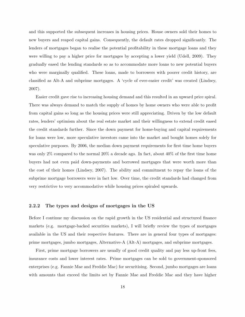
One major reason for the substantial increase in subprime mortgage issuance is that the sub-
prime mortgages were relatively profitable for issuers. As shown in Figure 2-1, the profitability of
subprime mortgage lending was especially high in the first four years of the 2000s (Weaver, 2008).
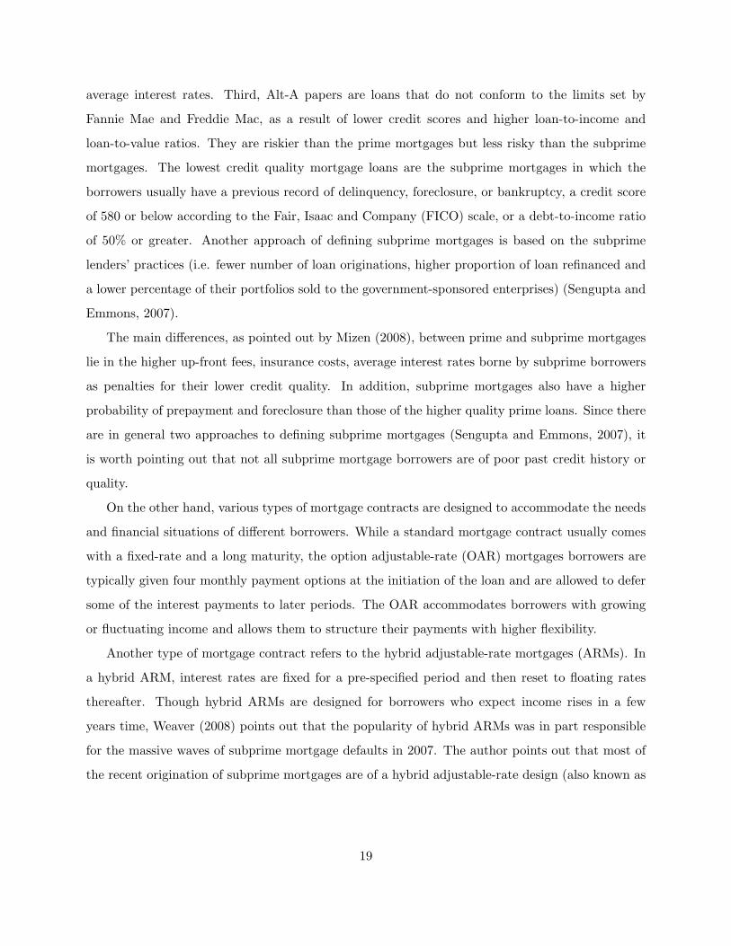
Jaffee (2008) notes that there were two periods of significant expansion of subprime credit. The
first period started in the late 1990s and lasted to the dotcom crisis in 2001. The second period
lasted between 2002 and 2006 (as shown in Figure 2-2). In particular, Jaffe (2008) notes that,
during the second period of expansion between 2002 and 2006, annual loan volumes of subprime
mortgages were over US$600 billion in 2005 to 2006, accounting for over 20% of the total annual
mortgage issuances. During the period between 2001 and 2005, the number of subprime loans
issued increased by about 450%, from 624,000 to 3,440,000, while the average subprime loan value
increased by 72%, from US$151,000 in 2001 to $259,000 in 2006. The total issued subprime mort-
gage loan values were US$94 billion in 2001, which rose more than 700% to US$685 billion in 2006
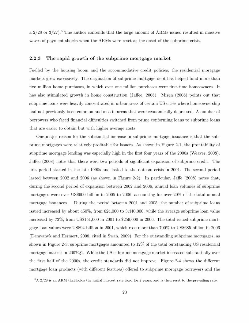
(Demyanyk and Hermert, 2008, cited in Swan, 2009). For the outstanding subprime mortgages, as
shown in Figure 2-3, subprime mortgages amounted to 12% of the total outstanding US residential
mortgage market in 2007Q1. While the US subprime mortgage market increased substantially over
the first half of the 2000s, the credit standards did not improve. Figure 2-4 shows the different
mortgage loan products (with different features) offered to subprime mortgage borrowers and the
6A 2/28 is an ARM that holds the initial interest rate fixed for 2 years, and is then reset to the prevailing rate.
20
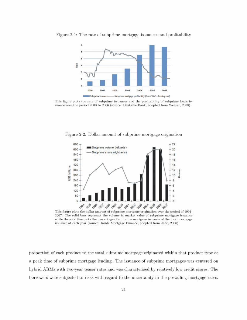
Figure 2-1: The rate of subprime mortgage issuances and profitability
This figure plots the rate of subprime issuances and the profitability of subprime loans is-suance over the period 2000 to 2006 (source: Deutsche Bank, adopted from Weaver, 2008).
Figure 2-2: Dollar amount of subprime mortgage origination
This figure plots the dollar amount of subprime mortgage origination over the period of 1994-2007. The solid bars represent the volume in market value of subprime mortgage issuancewhile the solid line plots the percentage of subprime mortgage issuance of the total mortgageissuance at each year (source: Inside Mortgage Finance, adopted from Jaffe, 2008).
proportion of each product to the total subprime mortgage originated within that product type at
a peak time of subprime mortgage lending. The issuance of subprime mortgages was centered on
hybrid ARMs with two-year teaser rates and was characterised by relatively low credit scores. The
borrowers were subjected to risks with regard to the uncertainty in the prevailing mortgage rates.
21
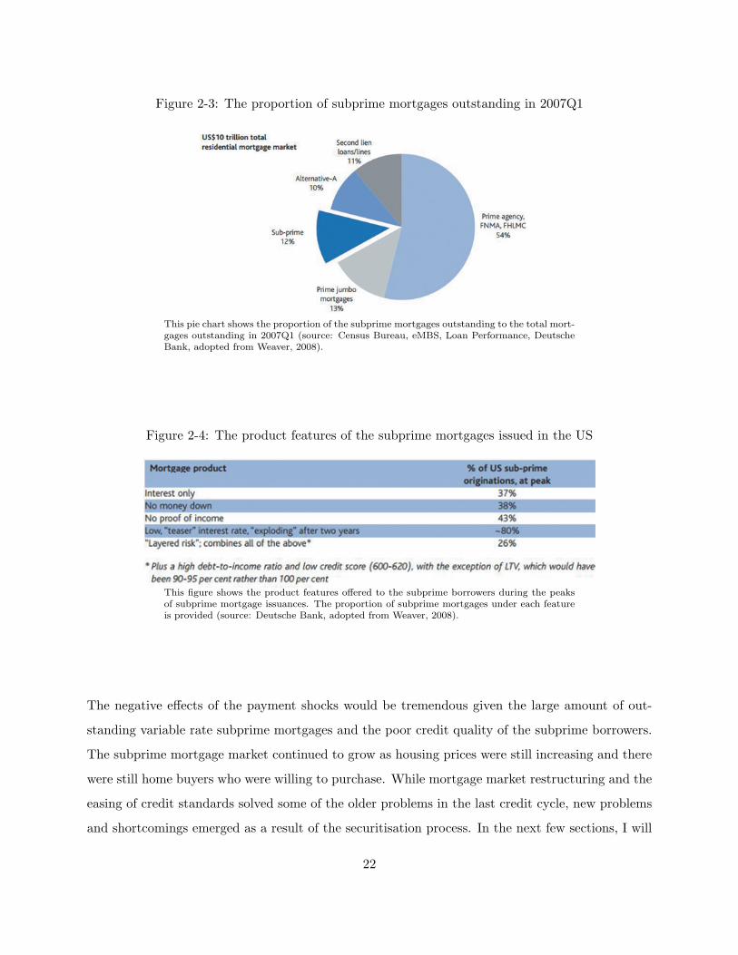
Figure 2-3: The proportion of subprime mortgages outstanding in 2007Q1
This pie chart shows the proportion of the subprime mortgages outstanding to the total mort-gages outstanding in 2007Q1 (source: Census Bureau, eMBS, Loan Performance, DeutscheBank, adopted from Weaver, 2008).
Figure 2-4: The product features of the subprime mortgages issued in the US
This figure shows the product features offered to the subprime borrowers during the peaksof subprime mortgage issuances. The proportion of subprime mortgages under each featureis provided (source: Deutsche Bank, adopted from Weaver, 2008).
The negative effects of the payment shocks would be tremendous given the large amount of out-
standing variable rate subprime mortgages and the poor credit quality of the subprime borrowers.
The subprime mortgage market continued to grow as housing prices were still increasing and there
were still home buyers who were willing to purchase. While mortgage market restructuring and the
easing of credit standards solved some of the older problems in the last credit cycle, new problems
and shortcomings emerged as a result of the securitisation process. In the next few sections, I will
22

explain the securitisation process and discuss how it relates to the recent crises.
2.2.4 The securitisation of mortgage loans and the CDOs
The securitisation of mortgage loans refers to the process of packaging cash flows (both interest and
principal) from the borrowers of mortgage loans and then selling these cash flows to underwriters
for the issuance of new securities. There are, in general, two types of securitisation: pass-through
and tranched securitisation.
In a pass-through securitisation, the cash flows of the underlying mortgages are ‘passed through’
to the investors who hold the MBSs. The introduction of pass-through securities dates back 40
years to a time when the underlying mortgages and MBSs were all guaranteed by the US govern-
ment.7 It was not long until Fannie Mae and Freddie Mac started to run their own non-government
guaranteed MBS programme. Even though these MBSs were not government guaranteed, they
are commonly thought as default risk free because the two enterprises guarantee the interest and
principal payments (Jaffee, 2008).
The second type refers to the tranched securitisation in which some investors hold more senior
claims than others within a subordination structure. Like the mechanism of a waterfall, in the
event of default, losses are absorbed by the lowest priority class of investors and the unabsorbed
losses are then absorbed by the next lowest priority class, and so on. The structure allows investors
of various tranches to take on different levels of risks (i.e. the most senior tranche has the highest
credit quality while the lowest residual equity tranche are the riskiest). Apart from the structure,
these tranched structured finance products use credit enhancing extensively to provide additional
insurance.
Looking at the mortgage loan securitisation, in 2001 about 46% of the subprime mortgages and
18% of the Alt-A mortgages were securitised. Most of these MBSs were ‘agency’ issues that had
higher credit quality and regulations. Over time, the proportion of ‘non-agency’ issues of MBSs
grew significantly with the largest growth in the subprime and Alt-A loan sectors. By 2006, about
75% of the subprime loans and 91% of the Alt-A loans were securitised. As shown in Figure 2-5,
the amount of outstanding residential mortgage-backed securities (RMBS) account for the largest
7The MBSs were issued by the Government National Mortgage Association (Ginnie Mae; GNMA), a govern-ment agency within the US Department of Housing and Urban Development. The underlying mortgages must begovernment guaranteed.
23
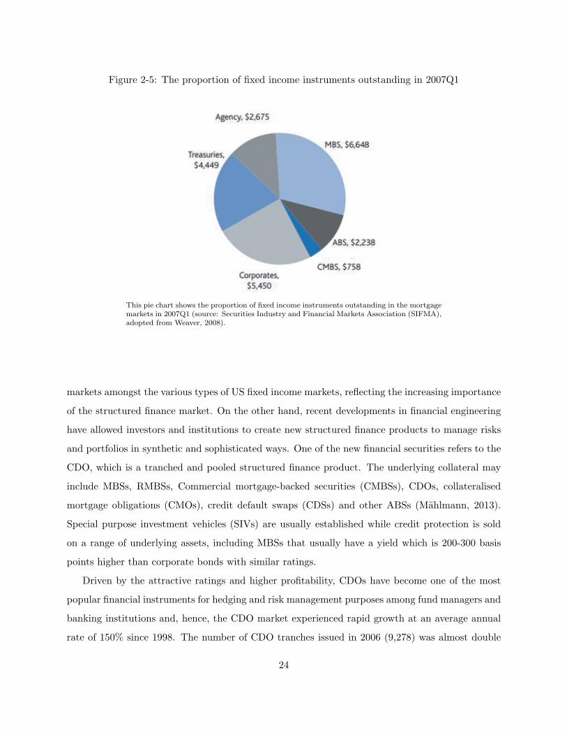
Figure 2-5: The proportion of fixed income instruments outstanding in 2007Q1
This pie chart shows the proportion of fixed income instruments outstanding in the mortgagemarkets in 2007Q1 (source: Securities Industry and Financial Markets Association (SIFMA),adopted from Weaver, 2008).
markets amongst the various types of US fixed income markets, reflecting the increasing importance
of the structured finance market. On the other hand, recent developments in financial engineering
have allowed investors and institutions to create new structured finance products to manage risks
and portfolios in synthetic and sophisticated ways. One of the new financial securities refers to the
CDO, which is a tranched and pooled structured finance product. The underlying collateral may
include MBSs, RMBSs, Commercial mortgage-backed securities (CMBSs), CDOs, collateralised
mortgage obligations (CMOs), credit default swaps (CDSs) and other ABSs (Mahlmann, 2013).
Special purpose investment vehicles (SIVs) are usually established while credit protection is sold
on a range of underlying assets, including MBSs that usually have a yield which is 200-300 basis
points higher than corporate bonds with similar ratings.
Driven by the attractive ratings and higher profitability, CDOs have become one of the most
popular financial instruments for hedging and risk management purposes among fund managers and
banking institutions and, hence, the CDO market experienced rapid growth at an average annual
rate of 150% since 1998. The number of CDO tranches issued in 2006 (9,278) was almost double
24

the number of tranches issued in 2005 (4,706) (see Benmelech and Dlugosz, 2009). By 2005, it was
estimated that the overall CDO market was over $1.5 trillion in market value (Celent Consultant,
2005). The total amount of CDO issuances peaked in the first half of 2007 with a volume of $345
billion (SIFMA, 2010) while about 60% of the global CDOs issuance has concentrated in CDOs
with ABSs as collateral (Mahlmann, 2013).
2.2.5 Problems with the securitisation of mortgage loans
While the securitisation process allows lenders to acquire immediate liquidity through selling mort-
gages to underwriters, it also creates a number of problems and encourages risk-taking behaviour.
First, in the case of a single layer ABS securitisation, when an asset is securitised with its cash
flows repackaged, they are usually taken off the balance sheets of the lenders (a feature of pass-
through securities). Risks in the loan assets are effectively transferred from the original lenders to
the underwriters (buyers) during the transaction. As the default risks are no longer borne by the
lenders, they are keen to make more mortgage loans to borrowers than they could have based solely
on credit profiles. The underwriters, who bought the loan assets, put them into trusts and issue
MBSs to fund the purchases. In the process of MBS issuance, underwriters have again effectively
transferred the credit risks to the MBS investors and made profits within a short time (Udell,
2009). Therefore, underwriters’ incentives to monitor the borrowers’ credit quality are essentially
low. The process of securitisation creates a misalignment of risk and returns between borrowers
and lenders that in effect encourages risk-taking behaviour.
Second, securitisation creates a separation between mortgage lenders and borrowers, and severs
the problem of asymmetric information. The effective lender of the underlying mortgages of the
MBS is the investor who bought the MBS, rather than the original mortgage lender. Investors are
not able to accurately evaluate their risk exposure and make well-informed investment decisions
without detailed information on the collateral (e.g. on the real estate assets) and the credit quality
of the borrowers. The separation inevitably forces investors to over rely on statistical information
provided by the MBS issuers, such as the loan-to-value ratios, qualitative descriptions of the home-
owners’ creditworthiness and, most prominently, on the credit ratings issued by the rating agencies.
During tranquil periods of rising housing prices, this information alone is sufficient for evaluating
credit quality. However, when the economy slowed and the housing bubble was about to burst, the
25

statistical criteria were found to be largely inaccurate and resulted in substantial underestimation
of risks (Weaver, 2008). The function of monitoring the credit quality of loan borrowers by banks
or issuers became largely ineffective in the process of securitisation.
Third, the credit rating system may be subject to potential bias and conflicts of interest. First,
the information which rating agencies relied on may not have been accurate or sufficient to ob-
jectively evaluate the risks. Second, the rating agencies face potential conflicts of interest as the
rating fees are paid by the same underwriters or financial institutions that issued the structured
securities. Agencies usually compete with each other for rating businesses. Tighter and more pru-
dent rating standards on the MBSs would probably hurt the sales of MBSs and the profitability of
the underwriters (Udell, 2009). Underwriters may be prone to select rating agencies that are less
stringent and strict in assigning ratings so that higher valuation and liquidity can be achieved at
the time of issuance and release. The result was a substantial underestimation of risk.
On the other hand, one important complication of securitisation in relation to the recent crisis
refers to the extensive use of structured securities (e.g. ABSs, CDSs, MBOs, etc.) as the underlying
collateral for the CDO tranches.8 Under wrong actuarial assumptions, the rating agencies largely
overlooked the high correlations between tranches and systematically underestimated the risk in
CDOs (Jaffe, 2008; Weaver, 2008). Mezzanine bonds of low credit quality were allowed to be
pooled into new AAA-rated CDO bonds, which were then sold to investors as low risk fixed income
products. When house prices fell and the mortgage delinquency rates increased, the prices of
CDOs withered as the tranches were simultaneously shocked. A number of international financial
institutions, which were assured that the AAA rating provided sufficient protection, held large
subprime CDO portfolios. Therefore, the troubles in the US subprime mortgage markets and the
structured finance markets would not only affect the US financial markets but would also affected
a number of international markets.
8Mahlmann (2013) refers to those CDOs with structured finance products as underlying assets ABS-CDOs, whichrepresent the largest proportion of global CDO issuances.
26

2.3 The outbreak of the subprime crisis
2.3.1 The bursting of the US housing bubble
As mentioned in the previous sections, market restructuring, increasing housing demand, and the
fast-expanding subprime mortgage market were all underlying causes of the development of a
housing bubble in the US market.9 The housing bubble would burst when there were no longer any
investors or home buyers who were willing to buy homes. Meanwhile, the excess supply of houses
would drive the prices down. As shown in Figure 2-6, the S&P/Case-Shiller Home Price Composite
- 20 index, which tracks the average US housing prices, peaked in year 2006 and started to decline
in mid-2007. When the house prices fell, borrowers were reluctant to sell their homes as selling their
homes at lower prices result in negative equity and require paying additional collateral to lenders.
Therefore, the number of housing transactions decreased gradually. In 2006, there were 9% fewer
houses sold compared to that in 2005 while the price of the median home was just slightly lower
than that in 2005 (Lindsey, 2007). On the other hand, mortgage lenders became more cautious
in issuing new loans while appraisers, who assess the house values, also became more conservative
because there were fewer comparable house sales and that the house sales were usually made at
much lower prices. As the credit standards became more restrictive, the amount of mortgages and
houses sales declined excessively. This resulted in a downward spiral of housing prices.
2.3.2 The mortgages’ delinquencies and the failing structured finance market
Home buyers who financed their purchases with ARMs expected to sell their homes quickly to
capture capital gains. However, when the prices and housing sales started to decline, some of them
were reluctant to sell their houses and realise capital losses. After the expiration of the fixed-rate
period, they inevitably had to pay the higher prevailing interest rates. As shown in Figure 2-7,
the residential, commercial and total loans & leases delinquency rates (including both prime and
subprime grades of loans) started to rise from 2006 onwards. As the threat of mortgage defaults
heightened, the MBS prices declined sharply. The buy-side of the MBS market almost disappeared
and the valuation of the subprime CDOs became extremely difficult due to the lack of transparency
and the high uncertainty with regard to their collateral values (e.g. the value of the MBSs). Since
9Phillips and Yu (2011), using statistical techniques, document evidence of bubbles in US housing prices inFebruary 2002.
27
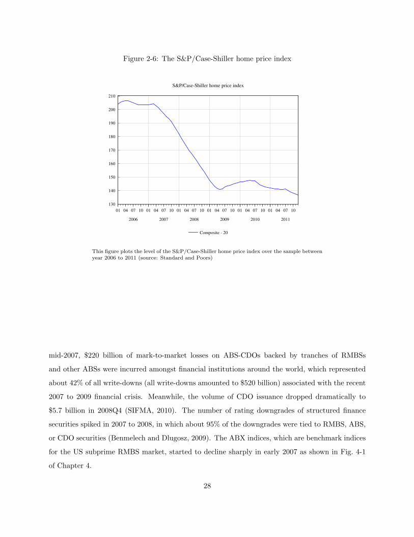
Figure 2-6: The S&P/Case-Shiller home price index
130
140
150
160
170
180
190
200
210
01 04 07 10 01 04 07 10 01 04 07 10 01 04 07 10 01 04 07 10 01 04 07 10
2006 2007 2008 2009 2010 2011
Composite - 20
S&P/Case-Shiller home price index
This figure plots the level of the S&P/Case-Shiller home price index over the sample betweenyear 2006 to 2011 (source: Standard and Poors)
mid-2007, $220 billion of mark-to-market losses on ABS-CDOs backed by tranches of RMBSs
and other ABSs were incurred amongst financial institutions around the world, which represented
about 42% of all write-downs (all write-downs amounted to $520 billion) associated with the recent
2007 to 2009 financial crisis. Meanwhile, the volume of CDO issuance dropped dramatically to
$5.7 billion in 2008Q4 (SIFMA, 2010). The number of rating downgrades of structured finance
securities spiked in 2007 to 2008, in which about 95% of the downgrades were tied to RMBS, ABS,
or CDO securities (Benmelech and Dlugosz, 2009). The ABX indices, which are benchmark indices
for the US subprime RMBS market, started to decline sharply in early 2007 as shown in Fig. 4-1
of Chapter 4.
28
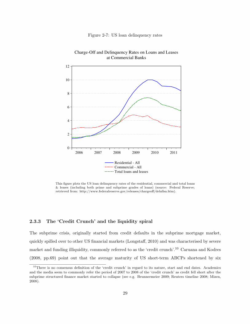
Figure 2-7: US loan delinquency rates
0
2
4
6
8
10
12
2006 2007 2008 2009 2010 2011
Residential - All
Commercial - All
Total loans and leases
Charge-Off and Delinquency Rates on Loans and Leases
at Commercial Banks
This figure plots the US loan delinquency rates of the residential, commercial and total loans& leases (including both prime and subprime grades of loans) (source: Federal Reserve;retrieved from: http://www.federalreserve.gov/releases/chargeoff/delallsa.htm).
2.3.3 The ‘Credit Crunch’ and the liquidity spiral
The subprime crisis, originally started from credit defaults in the subprime mortgage market,
quickly spilled over to other US financial markets (Longstaff, 2010) and was characterised by severe
market and funding illiquidity, commonly referred to as the ‘credit crunch’.10 Caruana and Kodres
(2008, pp.69) point out that the average maturity of US short-term ABCPs shortened by six
10There is no consensus definition of the ‘credit crunch’ in regard to its nature, start and end dates. Academicsand the media seem to commonly refer the period of 2007 to 2008 of the ‘credit crunch’ as credit fell short after thesubprime structured finance market started to collapse (see e.g. Brunnermeier 2009; Reuters timeline 2008; Mizen,2008).
29

days with outstanding ABCPs declines amounting to approximately $300 billion from August 2007
onwards.
In the literature, there is theoretical and empirical evidence that funding and market illiquidity
have played important roles in the subprime and the subsequent global financial crises. In the
following sections, we shall address a few important issues with regard to liquidity.
2.3.4 The SIVs and ABCPs
As pointed out by Brunnermeier (2009), banking institutions were subjected to higher funding
illiquidity risks because of their increasing reliance on shorter maturity instruments, such as ABCPs.
ABCPs are commercial papers that are collaterlised by assets, usually with a 30-day or 90-day
maturity. One particularly important use of ABCPs by banking institutions in relation to the
recent crisis was to fund the purchase of subprime structured finance securities in off-balance sheet
SIVs and conduits.11
Over the years, ABS-CDOs have gained considerable popularity among institutional investors
and banks for hedging and risk management purposes. Holding the CDO portfolios via off-balance
sheet conduits, these institutions funded their purchases of CDOs with the issuance of short-term
ABCPs, which require periodic roll-over (e.g. each month) (Brunnermeier, 2009). The maturity
mismatch between the long-term structured securities and the short-term ABCPs enables the in-
stitutions to profit from the yield differences. A protection mechanism for the SIVs is established
in that, if the ABCPs are insufficient to fund the CDOs, the owners of the SIVs are obliged to
provide additional funding via credit line facilities.
During the crisis, the funding liquidity of financial institutions shrank as the market wide default
risks increased and the banks’ external access to external funding was restricted. Investors were
unwilling to roll over their ABCPs resulting in a severe funding shortage in SIVs and conduits. As
shown in Figure 2-8, the ABCP spreads (calculated as the yield differentials between one-month
ABCPs and one-month Treasury bills) started to widen from mid-2007 onwards, and reached as
11In general, there are two types of SIVs. The first type refers to the self-standing SIVs that are essentiallyinvestment funds without connection to a commercial bank. The second type refers to SIVs that are wholly ownedand operated by a commercial or investment bank ,of which the SIVs are run by bank employees and protectedby credit line facilities provided by the same bank (Eichengreen, 2008). Self-standing SIVs are those vehicles thatpurchase longer-term assets financed by the issuance of ABCPs. The wholly owned SIVs are sometimes consideredas a tool by financial engineers to disguise and repackage loan assets, escaping the scrutiny of the regulatory body.In our discussion, we are referring to both types of SIVs.
30
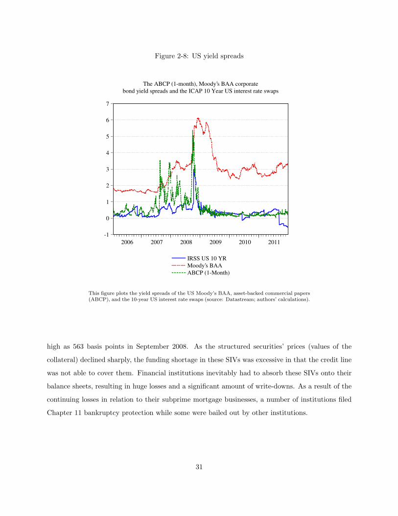
Figure 2-8: US yield spreads
-1
0
1
2
3
4
5
6
7
2006 2007 2008 2009 2010 2011
IRSS US 10 YR
Moody’s BAA
ABCP (1-Month)
The ABCP (1-month), Moody’s BAA corporate
bond yield spreads and the ICAP 10 Year US interest rate swaps
This figure plots the yield spreads of the US Moody’s BAA, asset-backed commercial papers(ABCP), and the 10-year US interest rate swaps (source: Datastream; authors’ calculations).
high as 563 basis points in September 2008. As the structured securities’ prices (values of the
collateral) declined sharply, the funding shortage in these SIVs was excessive in that the credit line
was not able to cover them. Financial institutions inevitably had to absorb these SIVs onto their
balance sheets, resulting in huge losses and a significant amount of write-downs. As a result of the
continuing losses in relation to their subprime mortgage businesses, a number of institutions filed
Chapter 11 bankruptcy protection while some were bailed out by other institutions.
31
2.3.5 The relation between market and funding illiquidity
Brunnermeier and Pedersen (2009) propose a theoretical model that explains the relation between
market illiquidity and traders’ funding illiquidity. It also explains how a reinforcing liquidity spiral
may arise in times of financial stress. In particular, during the crisis, the traders’ ability to provide
market liquidity was impaired because they faced losses in positions and larger margin requirements.
When markets become illiquid, margin requirements may be driven higher as lenders become more
conservative and prudent. In addition, the traders’ initial asset position may also incur losses.
The overall effects of the two forces further reduce the funding liquidity of the traders, resulting in
potential deleveraging and a ‘fire-sale’ of assets in which the liquidity spiral starts over again.
Empirical studies have examined the validity of the hypotheses presented in Brunnermeier and
Pedersen (2009) and have found consistent results that support the propositions of their model.
Frank et al. (2008) document evidence of significant increases in comovements between market
and funding illiquidity in the US financial system that are consistent with the liquidity spiral
conjecture. Boyson et al. (2010) document evidence of contagion in hedge funds and find that they
were exposed to some common risk factors associated with funding illiquidity. Gorton and Metrick
(2012) document evidence that the LIBOR-OIS spreads were associated with the changes in credit
spreads and the collateralised REPO rates. Their findings are consistent with Brunnermeier and
Pedersen (2009) in that, when the uncertainty with regard to bank solvency increased, the margin
requirements increased as a result of lower REPO collateral values. Longstaff (2010) finds evidence
of contagion from the US structured market to a number of US asset markets during the subprime
crisis. He further shows that contagion was associated with changes in various funding liquidity
variables, including: the ratios of trading volumes of financial stocks to the overall market, the
number of fails in REPO, and changes in ABCP yield spreads. Comerton-Forde et al. (2010)
find a significant relation between the funding constraints faced by NYSE specialists and the time
variation in market illiquidity, while Dick-Nielsen et al. (2012) find evidence of bond illiquidity
during the subprime crisis.
32

2.4 The similarities and differences between the recent and pre-
vious crises
The previous sections have discussed how the crisis evolved and addressed issues with regard to
the importance of market and funding illiquidity to contagion during the recent crisis. This section
briefly reviews the literature and will summarise the similarities and differences of the recent crisis
in comparison to previous crisis events.
Reinhart and Rogoff (2008) examine the early stage of the subprime crisis and 18 previous
post-war banking crises in a number of industrialised countries and have identified a few similarities
between the crisis episodes. In particular, they find significant increases in housing prices prior to
the crises and dramatic declines during and after the crises. They observe similar inverted V-shape
patterns in output growth prior to the crises. Claessens et al. (2010) also point out that the housing
price bubble prior to the subprime crisis is similar to those in the so-called Big Five banking crises.12
They also note that the default correlation on the outset of the subprime crisis was high provided
that a large proportion of domestic loan assets were denominated in foreign currencies, similar to
that during the East Asian crisis in 1997.
On the other hand, Claessens et al. (2010) point out that the subprime crisis was characterised
by the ‘explosion’ of opaque structured finance securities and the exceptionally high leverage (in
contrast to previous crisis studies). In addition, international markets have undergone substantial
market reforms and have become more integrated with larger increases in cross-border investments
than those in the previous crisis episodes. Reinhart and Rogoff (2008) find that the run-up of public
debts in the US ahead of the subprime crisis is lower than the average levels of previous events.
in addition, the authors note that the account deficits were on an increasing trend that was worse
than any previous crises.
2.5 The crisis subperiods
This section will discuss and define the different phases of the recent 2007 to 2009 crisis and it
will compare my crisis dates with those used in other studies. Our sample period covers the
12The Big Five banking crises refer to the banking crisis episodes in Finland (1991), Japan (1992), Norway (1987),Sweden (1991) and Spain (1977).
33
period of 19 January 2006 to 30 December 2011. Following the contagion literature, I will split the
sample into four subperiods: pre-crisis, subprime, global and post-crisis subperiods. This allows
us to detect significant contagion and facilitate comparison of empirical findings across periods of
different levels of volatilities and market performance. Since there are no exact dates that best
define the crisis outbreak13, I will base my criteria of subperiod selection on historical events and
market performances.14
For the pre-crisis subperiod, I will follow Longstaff (2010) and define the pre-crisis subperiod
as the period between 20 January 2006 and 29 December 2006, during which the domestic US
financial markets were relatively tranquil and free from substantial shocks and volatilities. Following
Longstaff (2010), the subprime crisis subperiod is defined as the period between 2 January 2007
and 31 December 2007.15 The subprime crisis subperiod is characterised by significant mark-to-
market losses on the balance sheets of financial institutions worldwide in relation to their subprime
mortgage businesses and structured credit instruments (e.g. HSBC, New Century Financials, Bear
Stearns’ bailing out of its structured credit hedge funds in June 2007). While some researchers
define July 2007 as the start of the subprime crisis (credit crisis or liquidity crisis)16, I define
January 2007 as the beginning date of the subprime crisis subperiod due to the fact that this is
precisely when the ABX indices started to decline sharply. In fact, in early 2007, the declines in
ABX indices’ prices already reflected the shocks in the structured finance market that had not
yet been transmitted to other markets and fully reflected in other stress indicators (e.g. the TED
spreads, the LIBOR-OIS spreads, the ABCP yield spreads or the Moody’s Coporate bond yield
spreads). Therefore, this definition of the subprime crisis enables me to focus on the spillovers of
idiosyncratic shocks from the US structured finance market and allows my results to be readily
comparable to those documented by Longstaff (2010).
The global crisis subperiod is defined as the period between 2 January 2008 and 31 March
2009, during which a number of financial institutions (i.e. Lehman Brothers) collapsed and were
13Not only are there no consensus start or end dates for the crisis episodes, some researchers do not distinguishbetween the subprime and the global crisis, and sometimes commonly refer them as ‘the 2007 to 2009 financial crisis’,‘global crisis’, ‘credit crisis’ or ‘liquidity crisis’ (see, for example, Flannery et al., 2013; Bekaert et al., 2011).
14The historical evolution of the financial crises from the Federal Reserve Bank of St. Louis web site -http://timeline.stlouisfed.org/ is useful in this regard.
15Reinhart and Rogoff (2008) also define 2007 to 2008 as the subprime mortgage financial crisis.16See, for example, Milunovich and Tan (2013); Edmonds et al. (2010); Flannery et al. (2013), for the crisis period
defined as 2007Q3 to 2009Q3; Olson et al. (2012), for a structural break analysis on the US LIBOR-OIS spreads withthe break in August 2007.
34
bailed out. While Longstaff (2010) define the entire year 2008 as the global crisis phase, we
further extend the global crisis subperiod to include 2009Q1 based on the fact that the US and
the G5 international equity markets crashed in late 2008 and tumbled in 2009Q1. Lastly, I will
include a post-crisis window that covers the period between 2 September 2009 and 28 December
2011. The observations between April 2009 and August 2009 are intentionally omitted as the
ABX BBB and BBB- indices were considerably thinly-traded. The daily return series during this
subsample contained a number of consecutive zero returns, thus creating near singularity problems
in regressions. Nonetheless, the post-crisis subperiod is not completely free of shocks and partly
covers the ongoing European Sovereign Debt Crisis.
2.6 Conclusions
This chapter has reviewed the major issues with regard to the contexts, causes, consequences and
evolution of the recent subprime and the subsequent global financial crises. In particular, it has
discussed how the housing boom, the ever-easier credit standards, and the securitisation process
explain the rapid growth in the US structured finance market and the substantial increases in the
issuances of RMBSs, ABSs, and CDOs. It then explained how the bursting of the housing bubble
triggered the waves of mortgage delinquencies and the subsequent failure of the structured finance
market. Important issues with regard to funding and market illiquidity have been addressed along
with supportive empirical evidence. It has also discussed and defined the crisis subperiods, based
on historical events and market performances, for use in the empirical investigation in subsequent
chapters.
This chapter provides comprehensive background information on the role played by the US
structured finance market in the recent crisis. The next chapter will review the contagion literature
with a focus on the definitions, theoretical basis, empirical methodologies and empirical findings.
35

THIS PAGE INTENTIONALLY LEFT BLANK
36

Chapter 3
Literature Review on Financial
Contagion
3.1 Introduction
Despite the fast-expanding empirical literature on financial contagion, there is still widespread
disagreement over the working definitions of contagion among researchers (Forbes and Rigobon,
2002). Since the widespread disagreement in definition inevitably makes comparison across findings
relatively difficult, it is worthwhile investigating how the different empirical methodologies are
motivated from specific definitions and how the findings should be interpreted.
In the literature, there are various excellent surveys on the theoretical and empirical aspects
of contagion research (see, for example, Dornbusch et al., 2000; Kaminsky et al., 2003; Pericoli
and Sbracia, 2003; Dungey et al., 2005). Motivated by the recent crisis events, a large number
of empirical studies have been published in an attempt to detect the occurrence of contagion and
explain its transmission mechanism. In this chapter, I shall review the theoretical and empirical
contagion literature and address some of the major issues and recent developments in contagion
research, with a particular focus on the transmission mechanism, the empirical methodologies, and
the empirical evidence.
This chapter is structured as follows. Section 2 reviews the working definitions of financial
contagion. Section 3 reviews a few major transmission mechanisms of contagion. Section 4 surveys
the empirical literature and reviews a few widely-acknowledged empirical methodologies. Section
37

5 summarises the empirical evidence on contagion and Section 6 concludes.
3.2 The working definitions of financial contagion
Financial contagion can be broadly understood as the spread of adverse market disturbances from
a shocked market to another (Dornbusch et al., 2000). Pericoli and Sbracia (2003) summarise and
propose a useful classification of contagion definitions that is commonly referenced in the literature,
as follows:
1. Contagion is a significant increase in the probability of a crisis in one country, conditional on
a crisis occurring in another country (Dornbusch et al., 2000).
2. Contagion arises when volatilities of asset prices transmit from the country of crisis to another
country (Edwards, 1998).
3. Contagion occurs when cross-country comovement of asset prices increases and the higher
comovement cannot be explained by fundamentals.
4. Contagion is a significant increase in comovements of prices and quantities across markets,
conditional on a crisis in one market (Dornbusch et al., 2000).
5. Contagion occurs when the transmission channel intensifies or changes after a shock in one
market or country (Forbes and Rigobon, 2002).
Definition 1 centers on the idea of a significant increase in the probability of a crisis conditional
on a crisis event. Definitions 2, 3 and 4 are somewhat similar in the sense that they more or less
encompass the notion of market comovements, such as volatilities, asset returns, trade or financial
flows. Definition 5 focuses on the sudden changes in the shock transmission mechanism during a
crisis.
Note that the working definitions of contagion have changed over time. Earlier studies on
contagion did not distinguish between contagion and interdependence (Pericoli and Sbracia, 2003).
Forbes and Rigobon (2002) introduce a more stringent definition of contagion by distinguishing
strictly between contagion and interdependence. According to the authors, interdependence is the
degree of normal comovement between two or more markets during a tranquil period and should
38

be taken into accounted; that is, only when there are significant increases in return comovements
during a crisis does contagion exist. It is, therefore, necessary to split the samples into ‘tranquil’
and ‘crisis’ subperiods and examine the changes in correlation coefficients across the subperiods.
Kaminsky et al. (2003) define contagion as the immediate short-term transmission of shocks across
financial markets, which occur in a ‘fast and furious’ way. The authors define the gradual effects
of the negative consequences brought on the crises as spillovers instead of contagion. Pericoli and
Sbracia (2003) point out that contagion may not necessarily be ‘fast and furious’ and immediate,
which is consistent with Longstaff’s (2010) findings of contagion travelling from the US structured
finance market to other US financial markets within trading weeks.
In this thesis, my working definition of contagion is consistent with Forbes and Rigobon (2002)
and distinguishes between contagion and interdependence. Following Longstaff (2010), I do not
rule out the possibility that contagion may not be ‘fast and furious’.
3.3 The mechanisms and channels of transmission of contagion
With regard to financial contagion, three major research questions are commonly addressed. First,
researchers are keen to identify and understand the possible channels and mechanisms in which
shocks transmit during a crisis. Second, as an extension to the first research question, the second
research question examines whether the identified channels and mechanisms may change during
a crisis; that is, whether the transmission channels may discontinue, strengthen or become active
only during crisis. Third, researchers seek to provide implications to various market users and
policymakers in establishing effective measures to prevent and contain the negative consequences
of the crisis events. In addition, empirical studies are important because they also provide important
implications to the investment community with regard to the effectiveness of international portfolio
diversification. Any significant increases in market comovements during the crisis temper the
benefits of international diversification and leave investors exposed to substantial risks.
In the following sections, I will review and summarise various widely-acknowledged causes and
transmission mechanisms of contagion in an intuitive manner. I follow the structure and classi-
fication of the survey by Dornbusch et al. (2000) and summarise the fundamental and investor
behaviour related causes.
39
3.3.1 Fundamental causes
The fundamental causes of contagion commonly refer to the spillovers of shocks through structural
changes in economic circumstances, trade linkages, financial linkages and competitive devaluations.
The fundamental causes are closely related to market integration in which a structural change in a
country induces shocks commonly experienced by many other countries. This may include struc-
tural shifts in the economy or the strengthening of some major currencies. Common shocks may
trigger comovement in asset prices across international markets (Dornbusch et al., 2000). Shocks
may transmit via the trade linkages that result in competitive devaluations. During a crisis, the
shocked country may experience sharp depreciations in its currency, declines in asset prices and
large capital outflows, which in turn make its products relatively cheaper compared to its competi-
tors internationally. The trading partners of this country, facing the cheaper products from the
shocked country, may voluntarily devalue their currencies in order to maintain the competitiveness
of their own exports resulting in higher comovements in asset prices via trade linkages.
The second fundamental cause refers to the shock transmission via financial linkages in which
direct financial effects spread across markets during a crisis. Some of the financial effects include
the reduction in trade credits, foreign direct investments and capital flows (Dornburch et al., 2000).
When a country is shocked, the other trading partners are affected due to their limited ability to
invest abroad and extend credit. In addition, this may also result in declines in the availability
of capital, higher costs of borrowing and may eventually lead to increased comovements in asset
prices.
3.3.2 Investors-related causes
Apart from the fundamental causes, investors’ related causes focus primarily on the role of investors
in shock transmission, which includes the effects of herding, liquidity shocks, information asymme-
tries (Kiyotaki and Moore, 2002), multiple equilibria and perception about changes in the rules of
financial transactions (Kaminsky et al., 2003).
The first investor related cause relates closely to the information transmission channel, in which
the arrival of economic news directly affects the collateral values or cash flows in other markets
(Kaminsky et al., 2003). This channel is consistent with the Efficient Market Hypothesis (EMH), in
which any new market information will be absorbed and reflected in the asset prices immediately,
40

and the contention that contagion should be ‘fast and furious’ and immediate. In other words,
contagion is a direct consequence of the transmission of market information or economic news from
the shocked market to other markets.
The second investor related cause of contagion relates closely to funding liquidity. In the model
proposed by Shleifer and Vishny (1997), when a shock lowers the asset returns in one country,
risk-averse arbitrageurs will liquidate their positions in other countries to meet the capital outflows
and avoid further losses, which is referred to as a ‘fire sale’. Calvo (1998) suggests that investors
may liquidate their assets to meet the increasing margin requirements during crisis and may be
prone to sell foreign assets in which the prices have not yet declined drastically in their portfolios.
Allen and Gale (2000) propose a model that focuses on the role of commercial banks in shock
transmission. The authors argue that financial shocks cause banks to liquidate cross-holdings
across regions leading to shortfalls of funding liquidity in other regions. Kaminsky and Reinhart
(2000) also share similar views with Allen and Gale (2000) and point out that foreign banks may
tighten up credit lines and call back loans in order to rebalance their overall risk exposure during a
crisis. In addition, Longstaff (2010) examines trading intensity in US financial stocks, the number
of fails in the REPO market and the size of the ABCP market, and finds evidence that the shocks
from the US structured finance market translated into subsequent higher funding illiquidity.
The third investor related cause refers to the way in which an individual investor follows the
behaviour of a precedent individual without regard to his own information, which is commonly
referred to as herding. Bikchandamn et al. (1998) propose a model of observational learning and
a theory of informational cascade that seeks to uncover the relation between signals from actions
by precedents, private information and private signals. An informational cascade occurs when
an individual disregards his private information but decides to follow the signals given by the
actions of his precedents. Note also that a person who follows others has a positive externality
of inducing others to follow the herd (Banerjee, 1992, cited in Kaminsky et al., 2003). During a
crisis, when asset prices have collapsed and liquidity has evaporated, institutional investors might
liquidate and sell their asset positions to meet their capital outflows. Individual investors may
follow without regard to their own knowledge about the markets, giving rise to further downside
comovements of asset prices. Calvo and Mendoza (2000) propose a model in which there are large
fixed costs associated with gathering and processing country-specific information. The existence of
41
the fixed costs allows economies of scale to be enjoyed by informed investors. When uninformed
investors observe the short positions of these informed investors, they are unable to determine
whether the short positions are caused by margin calls or other negative market information on the
fundamentals. The uninformed investors may follow the informed investors and enter into short
positions, resulting in herding effects and asset comovements.
The investors related cause with regard to information asymmetry focuses on the investors’
expectations and on the fact that investors have imperfect market information. In general, investors
are informed about the markets based on some composite financial indicators and make their
investment decisions accordingly. However, these indicators may not reflect accurately the situation
with regard to the severity of crisis events in an individual country. Investors formulate their
expectations rationally and infer that crises will hit their own countries, thus leading to possible
herding effects and comovement in asset prices.
Other investors’ related causes include multiple equilibria and changes in the market rules.
For multiple equilibria, a crisis in one country may force other countries into bad equilibria. In
other words, changes in investors’ expectation are self-fulfilling and move other countries into new
equilibria. For changes in the rules, this refers to the changes in the assessment of the rules and ways
in which financial transactions take place across countries and markets. One example mentioned
in Dornbusch et al. (2000) refers to the increasing doubt towards the International Monetary Fund
(IMF) in its ability to bail out distressed countries as the lender of last resort.
3.3.3 The risk premia transmission channel
The risk premia transmission channel refers to the comovements of asset prices that occur as a
result of changes in risk premia after a crisis event has taken place. An idiosyncratic shock to
one market results in subsequent changes in investors’ risk aversion and increases in risk premia
required by investors in other markets.
Recent studies document a significant role on market illiquidity risks in asset pricing (see, for
example, Amihud, 2002; and Acharya and Pedersen, 2005). Significant time variations in market
illiquidity risk premia and evidence of ‘flight-to-liquidity’ have been documented. Longstaff (2004)
finds significant liquidity premia in the yield spreads between the more liquid US Treasury bonds
over the Refcorp bonds suggesting some market liquidity components in Treasury bonds. Liu et al.
42
(2006) also find significant time-varying liquidity premia in the US Treasury bonds over the period
between 1988 and 2002. These empirical findings suggest that investors have certain liquidity
preferences and that ‘flight-to-safety’ phenomenon may be driven by liquidity, apart from credit
risk concerns. In other words, the increase in market illiquidity risks during a crisis might have
considerable impacts on the investors’ risk aversion and result in subsequent systematic ‘flights’ to
liquid assets. On the other hand, funding and market illiquidity may relate to each other closely.
Brunnermeier and Pedersen (2009) propose a model that describes the relation between funding
and market illiquidity in that traders’ funding illiquidity result in higher transaction costs and, in
turn, higher market illiquidity. The declines in asset prices as a result of market illiquidity further
temper the traders’ funding liquidity, result in a reinforcing liquidity spiral, and translate into
higher cross-market price comovements and spillovers of volatility.
Another widely-acknowledged risk premia refers to the credit risk premia that compensates for
default and counterparty risks. Vassalou and Xing (2004) find that equities’ credit risk premia are
systematic and significantly explain expected stock returns. Eichengreen et al. (2009) examine
the common factors that underlie the CDS spreads of major banks and find increasing importance
in these factors during the subprime crisis. In particular, these factors can be explained by the
heightening credit risks in the US banking industry. These findings support the contention of
significant time variations in credit risk premia in equity markets, especially in the financial sector.
The increase in credit risk premia may result in portfolio rebalancing and reinforce risk-averse
investors to ‘flight’ to less risky assets.
3.4 A survey of empirical methodologies of financial contagion
studies
In the literature, there are a number of empirical methodologies used in detecting the presence of
contagion. Given the disagreement on the working definitions of contagion, the interpretation of
empirical results is dependent on the specific working definitions adopted to facilitate systematic
comparison across findings. In this section, I review the literature with a focus on empirical
methodologies and highlight their implications to contagion research.
43
3.4.1 Probit and logit models
Eichengreen et al. (1996) published one of the earliest papers to examine contagion and shock
transmission. In particular, they studied cross-country contagion during various currency crisis
episodes. The authors formulate their working definition of contagion by relating contagion to the
significant increases in probability of speculative attacks in the domestic currency of one country,
conditional on a currency crisis in another country (see Definition 1). The contagion definition leads
naturally to an empirical framework that examines the relation between the occurrence of a binary
outcome (dependent variable) and the determinants of that outcome (independent variables); that
is, a probit or logit regression framework. In a probit model, the conditional probability of observing
a desired outcome of the dependent variable (πi) is written as:
πi = Φ(X ′γ), (3.1)
where Φ(·) is the cumulative distribution function (CDF) of the standard normal distribution
ensuring that πi stays between 0 and 1, X ′ is a vector of independent variables while γ is a vector
of coefficients.
Using a panel of quarterly data of macroeconomic and currency indices covering 20 industrial
countries over the period between 1959 and 1993, the authors examine whether the currency crisis
in country j translates into a higher probability of observing a currency crisis in other countries.
Practically, to define the occurrence of a currency crisis, the authors construct an index (EMPi,t)
that proxies for the pressure of speculative attacks by computing the weighted averages of the
exchange rate changes, reserve changes and interest rate changes as follows:
EMPi,t = α∆ei,t + β∆(ii,t − iG,t) + λ∆(ri,t − rG,t), (3.2)
where ei,t is the exchange rate, ii,t is the short interest rate (as a benchmark), and ri,t is the ratio
of international reserves of country i. The subscript G denotes that it is a German variable. α,
β and λ are weights while ∆ is a symbol for change. The weights are computed by equating the
volatilities of the three components in the EMP index to prevent any components from dominating
the index variations.
Currency crisis is defined as the realisation of extreme values in the EMP index. A crisis
44
dummy variable (Crisisi,t) is introduced, which takes on the value 1 when a currency crisis is
detected and 0 otherwise. The threshold value on the EMP index for a currency crisis is defined
as:
Crisisi,t = 1 if EMPi,t > µEMP + 1.5 σEMP ,
= 0 otherwise, (3.3)
where µEMP and σEMP are the sample mean and sample standard deviation of the EMP index.
The probit regression model is then written as follows:
Crisisi,t = ωD(Crisisj,t) + λI(L)i,t + εi,t, (3.4)
where I(L)i,t is an information set of 10 macroeconomic control variables. The null hypothesis is
no currency contagion, as given by ω = 0.
Using the same probit model framework, Caramazza et al. (2000) study the significance of
external and internal imbalances, financial weaknesses (as measured by reserve adequacy), trade
and financial linkages, institutional factors (exchange rate regimes and capital controls), and the
presence of nonlinear effects in explaining the currency crisis contagion, particularly during the
three major crisis episodes in the 1990s.
As pointed out by Dungey et al. (2005), empirical studies based on conditional probabilities
are attractive in that they allow researchers to generate probability estimates of contagion from
one country to another. The change in probability of observing a currency crisis can be calculated
by: Φ(Z1)−Φ(Z0) where Z1 = ω + λI(L)i,t and Z0 = λI(L)i,t. However, Dungey et al. (2005) also
notes that the use of dummy variables in general leads to losses of sample information, inefficient
parameter estimates and thus a loss of power in the test.
3.4.2 GARCH models
An extensively researched area of contagion refers to the examination of spillovers of volatilities
across markets during a crisis (see Definition 2). Motivated by the fact that return volatilities tend
to cluster and spike during market distress, generalised autoregressive conditional heteroskedastic
(GARCH) type models are particularly useful in modelling the dynamics of conditional volatilities
45

and are often used to study the possible transmission of volatilities across markets. In this section, I
review a few seminar papers on the spillovers of volatilities and provide details on the specifications
of the GARCH type models used.
A seminal paper by Engle et al. (1990) investigates whether the conditional volatilities in intra-
day exchange rates exhibited ‘heat wave’ or ‘meteor shower’ behaviour.17 Using per hour volatilities
of four major economic segments (New York, Tokyo, Pacific and Europe), the authors test whether
the conditional volatilities in one market predict those in other market segments. Empirically,
they employ a GARCH(1,1) model and formulate the conditional volatility functions as a vector
autoregressive model to test for the cross-market dynamics. The main model specification is as
follows:
εi,t|ψi,t ∼ N(0, hi,t) for i = 1, 2, ..., n.
hi,t = ωi + βihi,t−1 +i−1∑j=1
αijε2j,t +
n∑j=i
αijε2j,t−1. (3.5)
In the GARCH model, the conditional volatilities of market i are dependent on its own lag (the
second term), the contemporaneous conditional volatilities of the closed market segment (the third
term) and the lagged conditional volatilities of the remaining markets. The heat wave null hy-
pothesis is that the αij are jointly equal to zero; that is, there are no volatility spillovers. The
authors then compute the impulse responses of the conditional volatilities by rewriting the equa-
tion as a vector of moving averages with infinite order. The empirical findings reject the heat wave
hypothesis and show that Japanese news had the largest magnitude of volatility spillovers.
Engle (2002) proposes a new class of multivariate GARCH estimators, called the Dynamic
Conditional Correlation GARCH (DCC GARCH) model, as a generalisation to the Bollerslev (1990)
constant conditional correlation (CCC) estimator. The estimation of the DCC MGARCH model
involves first estimating univariate GARCH models on individual time series to obtain consistent
estimates of time-varying conditional volatilities, and then using those estimates to estimate the
17The authors utilise meteorological analogies and relate the ‘heat wave’ hypothesis to volatilities that have onlycountry-specific autocorrelation while ‘meteor shower’ for volatilities that have cross-market intra-daily spillovers ofvolatilities.
46
correlation parameters. The main specification of the DCC GARCH model is as follows:
rt|Ωt−1 ∼ N(0, DtHtDt),
D2t = diagωi+ diagκi • rt−1r
′t−1 + diagλi •D2
t−1,
εt = D−1t rt, (3.6)
Qt = S • (ιι′ −A−B) +A • εt−1ε′t−1 +B •Qt−1,
Rt = diagQt−1QtdiagQt−1,
St = E[εtε′t],
where rt is a n× 1 vector of pre-whitened returns, St is the unconditional correlation matrix of the
residuals εt, • is the Hadamard product, ι is a vector of ones. Dt is a diagonal matrix comprises
of the standard deviations from individually estimated univariate GARCH models with the ith
element denoted as√hi,t while Qt is a positive semidefinite covariance matrix. The first equation
states that the pre-whitened returns have a normal distribution while the second equation shows
that the asset returns follow univariate GARCH processes.
The log-likelihood function for the DCC estimators is given by:
rt|Ωt−1 ∼ N(0,Ht),
L =− 1
2
T∑t=1
(n log(2π) + log |Ht|+ r′tH−1t rt),
=− 1
2
T∑t=1
(n log(2π) + log |DtRtDt|+ r′tD−1t R−1
t D−1t rt), (3.7)
=− 1
2
T∑t=1
(n log(2π) + 2 log |Dt|+ log |Rt|+ ε′tR−1t εt),
=− 1
2
T∑t=1
(n log(2π) + 2 log |Dt|+ r′tD−2t rt − ε′tεt + log |Rt|+ ε′tR
−1t εt).
The author proposes a few estimation methods that give consistent but inefficient estimates of
the model parameters, even though the covariance matrix is very large. The log-likelihood can be
decomposed into two parts: a volatility part and a correlation part.
47

L(θ, ϕ) = Lv(θ) + Lc(θ, ϕ), (3.8)
where the subscript v denotes the volatility component and c denotes the correlation component.
Practically, the volatility part is the sum of individual GARCH likelihoods:
Lv(θ) = −1
2
∑t
n∑i=1
(log(2π) + log(hi,t +r2i,thi,t
), (3.9)
which are maximised when each GARCH likelihood is maximised separately. Since the squared
residuals are not dependent on the parameters, the correlation part can be written as follows:
Lc(θ, ϕ) = −1
2
∑t
(log |Rt|+ ε′tR−1t εt). (3.10)
Practically, the DCC-GARCH estimator delivers the parameters that maximise the likelihoods:
θ = argmaxLv(θ), (3.11)
with the estimated parameters in D used to estimate the parameters (ϕ) in Rt:
maxϕ
Lc(θ, ϕ). (3.12)
The author shows that when the first step estimates are consistent, the second step will also
give consistent estimates, as long as the function is continuous in the neighborhood of the true
parameters.
The DCC-GARCH model continuously adjusts the correlation for the time-varying volatility
and thus the contagion tests are not subject to the heteroskedasticity bias, as pointed out by Forbes
and Rigobon (2002).
3.4.3 Correlation coefficient analysis
Correlation coefficient analysis is one of the most popular empirical approaches to detecting con-
tagion in the literature. The study of market comovements is motivated from the observation
that, when a crisis episode occurs, a number of markets are adversely affected in a consistent and
48

correlated manner, and are unexplained by the underlying fundamentals. The correlation coeffi-
cient analysis is convenient and practical because it provides direct implications to international
portfolio diversification and risk management. For instance, in times of increased market comove-
ments, diversification benefits brought about by holding international assets become less effective
and portfolio risks would be underestimated. The empirical methodology parallels Definition 3 in
which contagion is defined as significant increases in market comovements conditional on a crisis
event.
Forbes and Rigobon (2002) establish a stringent contagion definition that only a significant
increase in the correlation coefficient (after accounting for the normal degree of interdependence)
is evidence of contagion. The authors point out that the conditional correlation coefficient in-
creases when the volatilities of the shocked market have increased during a crisis, even when the
unconditional correlation coefficient remains constant. To this end, they propose a correction for
heteroskedasticity and show that contagion documented using conditional volatilities without the
adjustment is spurious. The heteroskedasticity correction is written as follows:
ρadj =ρ∗√
1 + δ[1− (ρ∗)2], (3.13)
where
δ =σhiiσlii
− 1. (3.14)
Here, ρadj is the heteroskedasticity-adjusted unconditional correlation coefficient while ρ∗ is the
conditional correlation coefficient. δ is the relative increase in variances during a crisis in which
σhii and σlii are the variances of returns of market i during the high and low volatilities periods,
respectively. δ represents a non-linear transformation to the conditional correlation.
The test for significant increases in correlation coefficients is thus formulated as in the following
null hypothesis:
H0 : ρadj = ρ∗, (3.15)
while the alternative hypothesis is written as follows:
H1 : ρadj > ρ∗. (3.16)
49
The t-statistics for testing the null hypothesis can be written as (Dungey et al., 2005):
t-stat =ˆρadj − ρ∗√1Th
+ 1Tl
, (3.17)
where Th and Tl refer to the number of observations during the high and low volatility subperiods,
respectively. The standard errors are derived from the asymptotic distribution of the estimated
correlation coefcients.
By contrast, Dungey et al. (2005) show that this bivariate correlation coefficient test can be
formulated within a regression framework in which the standard errors are the ordinary least square
standard errors whilst the approach of Forbes and Rigobon (2002) uses asymptotically adjusted
standard errors.
Corsetti et al. (2005) argue that the heteroskedasticity correction in Forbes and Rigobon (2002)
is based on unrealistic assumptions with regard to the idiosyncratic variance and may bias the result
towards finding no contagion at all. Pesaran and Pick (2007) point out that correlation tests may
suffer from an upward bias because of potential endogeneity in the variables. The authors also
point out that the splitting of ‘tranquil’ and ‘crisis’ periods is somewhat arbitrary and difficult to
justify. Dungey et al. (2005) note that tests based on correlation coefficients are conservative and
in general find no evidence of contagion.
3.4.4 Vector autoregressive models
A vector autoregressive (VAR) model treats all variables in the system endogenously, and each
variable is expressed as a function of its own lags and the lags of the remaining variables. A
reduced-form (RF) VAR(p) can be written as:
yt = α0 +A1yt−1 +A2yt−2 + · · ·+Apyt−p + ut, (3.18)
where
yt =
y1,t
y2,t...
yn,t
, α0 =
α1,t
α2,t
...
αn,t
, Ai =
a(i)1,1 a
(i)1,2 · · · a
(i)1,n
a(i)2,1 a
(i)2,2 · · · a
(i)2,n
......
. . ....
a(i)n,1 a
(i)n,2 · · · a
(i)n,n
ut =
u1,t
u2,t...
un,t
50
The RF VAR can be extended to include a set of exogenous regressors xt where xt = [x1,t, ..., xq,t]′
in a VAR(p) with q exogenous variables.
There are, in general, three different approaches to using the VAR model to test for contagion.
The first method refers to using the VAR model to filter (or pre-whiten) asset returns with some
exogenous macroeconomic variables and then using the residuals of the endogenous variables for
further analysis. Forbes and Rigobon (2002) apply a bi-variate VAR model with interest rates
as exogenous variables and study the heteroskedasticity-adjusted correlation across the pair of
residual series to test for the existence of contagion. Favero and Giavazzi (2002) study the spillovers
of devaluation expectations among member countries of the European Exchange Rate Mechanism
(ERM) within the European Monetary System (EMS). Using weekly Euro rate spreads, the authors
examine the distribution of the VAR residuals of the rate spreads and define non-linearity and
heteroskedasticity in the VAR residuals as shocks. The authors identify the unusually large residual
observations by dummy variables for each shock and use structural models (simultaneous equations)
to test for the existence of cross-market contagion.
Second, the VAR model allows researchers to evaluate the dynamics of the variables of interest
by computing impulse response functions. To show how it works, I rewrite the VAR equation as a
vector moving averages (VMA) of infinite order:
yt = µ+Φ(L)ut = µ+
∞∑j=1
Φjut−j,
In = (In −A(L))Φ(L). (3.19)
TheΦj represents a n by nmatrix of moving average coefficients of the RF VAR innovations at time
t− j. Φ(j)i,k measures the response of variable i to a previous unit shock in innovation k, occurring
in time t− j. The impulse responses can be shown graphically by plotting the Φ(j)i,k against j. Baig
and Goldfajn (1999) study contagion among five Asian countries during the Asian financial crisis
in 1997. Using a VAR model framework, impulse response results show that the Thai Baht had
a significant immediate impact on the Malaysian, Indonesian, and the Philippines currency rates,
which lasted for about four days.
One of the drawbacks with regard to the RF VAR model, despite its relative ease in identifica-
tion and implementation, is that the impulse response analysis does not provide relevant economic
51
meaning because the unit shock (RF VAR innovations) to the RF VAR system is a linear combi-
nation of the VAR endogenous variables’ structural shocks, which are not identified.18 Therefore,
to derive an economic interpretation of the impulse responses, one has to derive the structural
innovations by imposing sufficient restrictions to the system of equations to identify the structural
VAR model.
The third type of contagion test refers to the examination of block predictive power of the
independent variables over the contemporaneous dependent variables on the VAR functions via
the Granger-causality test. Longstaff (2010) estimates VAR(4) models using weekly domestic US
market variables as endogenous variables and the ABX indices’ returns as strictly exogenous re-
gressors. The F-tests of joint significance on the ABX factor loadings show that the lagged ABX
index returns Granger-caused the contemporaneous US market returns only in 2007 (i.e. during the
subprime crisis). The increases in predictive power of the lagged variables conditional on a crisis
event are consistent with increases in cross-market linkages and thus the existence of contagion.
3.4.5 Factor models
Dungey et al. (2005) review the empirical methodologies of contagion and propose a unified latent
factor model framework that encompasses a few widely-acknowledged empirical models of contagion
(see, for example, Corsetti et al., 2001; Dungey and Martin, 2001; Dungey et al., 2002a, b; Forbes
and Rigobon, 2002; Bekaert et al., 2005). Factor models are used extensively in the literature and
bring the benefit of the possibility of volatility decomposition while accounting for interdependence
between markets. According to Dungey et al. (2005), a general setting of a latent factor model,
assuming a hypothetical world with only two asset markets in which contagion transmits from
market 1 to 2, can be shown as follows:
18A structural VAR representation captures the dynamics and has impulse response functions expressed in terms ofthe structural innovations that provides relevant economic interpretation. A few common approaches for identificationrestrictions include the application of a Cholesky decomposition to the RF VAR innovation’s covariance matrix(the so-called Sims-Bernanke Decomposition, cited in Enders, 2003, p. 75) (or equivalently, the recursive causalordering identification), the short-run zero restrictions on the structural matrix A in the AB SVAR models, thelong-run restrictions on the cumulative impulse response function matrix (The Blanchard-Quah Decomposition, citedin Enders, 2003, pp. 82), etc. (For more details, please refer to Sims (1980); Stock and Watson (2001); and NBERSummer Institute (2008).
52

y(Pre)1,t = α1wt + β1u1,t,
y(Pre)2,t = α2wt + β2u2,t, (3.20)
y(Crisis)1,t = α1wt + β1u1,t,
y(Crisis)2,t = α2wt + β2u2,t + λu1,t, (3.21)
where the y(Pre)i,t and y
(Crisis)i,t represent the demeaned asset returns of asset market i at time t
during the pre-crisis and the crisis subperiods, respectively. wt refers to a latent (or observed)
world factor that affects the asset markets commonly while ui,t refers to an idiosyncratic factor
local to market i. The y(Crisis)2,t expression now allows for the contagious effects from asset market
1 by incorporating the idiosyncratic factor u1,t into the equation and, hence, a test of contagion
can be carried out by comparing the parameters across the pre-crisis and crisis models.
From Equation 3.21, the covariance between the returns of market 1 and 2 during the crisis
period can be written as:
cov[y(Crisis)1,t , y
(Crisis)2,t ] = α1α2 + λβ1. (3.22)
A change in covariance between the pre-crisis and crisis period can be written as:
cov[y(Crisis)1,t , y
(Crisis)2,t ]− E[y
(Pre)1,t , y
(Pre)2,t ] = λβ1. (3.23)
A test of contagion can be hence framed as a test of the restriction of λ = 0 in the crisis model
(see Dungey et al., 2002a, b; Dungey and Martin, 2004). In addition, the two asset market model
framework can be extended to include i markets in a multivariate setting and for simultaneous
53
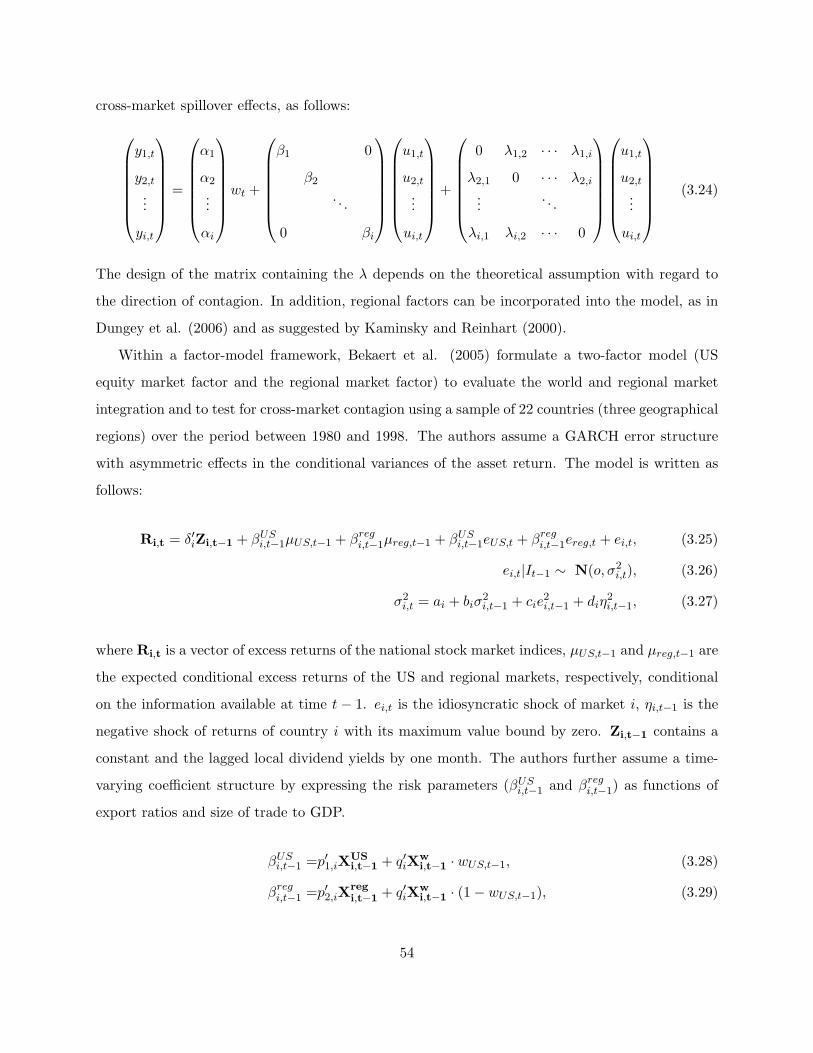
cross-market spillover effects, as follows:
y1,t
y2,t...
yi,t
=
α1
α2
...
αi
wt +
β1 0
β2. . .
0 βi
u1,t
u2,t...
ui,t
+
0 λ1,2 · · · λ1,i
λ2,1 0 · · · λ2,i...
. . .
λi,1 λi,2 · · · 0
u1,t
u2,t...
ui,t
(3.24)
The design of the matrix containing the λ depends on the theoretical assumption with regard to
the direction of contagion. In addition, regional factors can be incorporated into the model, as in
Dungey et al. (2006) and as suggested by Kaminsky and Reinhart (2000).
Within a factor-model framework, Bekaert et al. (2005) formulate a two-factor model (US
equity market factor and the regional market factor) to evaluate the world and regional market
integration and to test for cross-market contagion using a sample of 22 countries (three geographical
regions) over the period between 1980 and 1998. The authors assume a GARCH error structure
with asymmetric effects in the conditional variances of the asset return. The model is written as
follows:
Ri,t = δ′iZi,t−1 + βUSi,t−1µUS,t−1 + βregi,t−1µreg,t−1 + βUS
i,t−1eUS,t + βregi,t−1ereg,t + ei,t, (3.25)
ei,t|It−1 ∼ N(o, σ2i,t), (3.26)
σ2i,t = ai + biσ2i,t−1 + cie
2i,t−1 + diη
2i,t−1, (3.27)
where Ri,t is a vector of excess returns of the national stock market indices, µUS,t−1 and µreg,t−1 are
the expected conditional excess returns of the US and regional markets, respectively, conditional
on the information available at time t − 1. ei,t is the idiosyncratic shock of market i, ηi,t−1 is the
negative shock of returns of country i with its maximum value bound by zero. Zi,t−1 contains a
constant and the lagged local dividend yields by one month. The authors further assume a time-
varying coefficient structure by expressing the risk parameters (βUSi,t−1 and βregi,t−1) as functions of
export ratios and size of trade to GDP.
βUSi,t−1 =p
′1,iX
USi,t−1 + q′iX
wi,t−1 · wUS,t−1, (3.28)
βregi,t−1 =p′2,iX
regi,t−1 + q′iX
wi,t−1 · (1− wUS,t−1), (3.29)
54
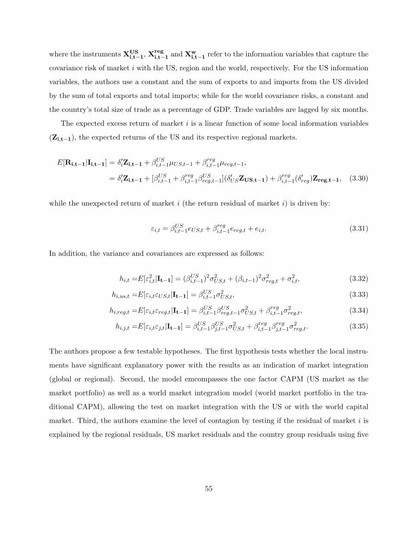
where the instruments XUSi,t−1, X
regi,t−1 and Xw
i,t−1 refer to the information variables that capture the
covariance risk of market i with the US, region and the world, respectively. For the US information
variables, the authors use a constant and the sum of exports to and imports from the US divided
by the sum of total exports and total imports; while for the world covariance risks, a constant and
the country’s total size of trade as a percentage of GDP. Trade variables are lagged by six months.
The expected excess return of market i is a linear function of some local information variables
(Zi,t−1), the expected returns of the US and its respective regional markets.
E[Ri,t−1|Ii,t−1] = δ′iZi,t−1 + βUSi,t−1µUS,t−1 + βregi,t−1µreg,t−1,
= δ′iZi,t−1 + [βUSi,t−1 + βregi,t−1β
USreg,t−1](δ
′USZUS,t−1) + βregi,t−1(δ
′reg)Zreg,t−1, (3.30)
while the unexpected return of market i (the return residual of market i) is driven by:
εi,t = βUSi,t−1eUS,t + βregi,t−1ereg,t + ei,t. (3.31)
In addition, the variance and covariances are expressed as follows:
hi,t =E[ε2i,t|It−1] = (βUSi,t−1)
2σ2US,t + (βi,t−1)2σ2reg,t + σ2i,t, (3.32)
hi,us,t =E[εi,tεUS,t|It−1] = βUSi,t−1σ
2US,t, (3.33)
hi,reg,t =E[εi,tεreg,t|It−1] = βUSi,t−1β
USreg,t−1σ
2US,t + βregi,t−1σ
2reg,t, (3.34)
hi,j,t =E[εi,tεj,t|It−1] = βUSi,t−1β
USj,t−1σ
2US,t + βregi,t−1β
regj,t−1σ
2reg,t. (3.35)
The authors propose a few testable hypotheses. The first hypothesis tests whether the local instru-
ments have significant explanatory power with the results as an indication of market integration
(global or regional). Second, the model emcompasses the one factor CAPM (US market as the
market portfolio) as well as a world market integration model (world market portfolio in the tra-
ditional CAPM), allowing the test on market integration with the US or with the world capital
market. Third, the authors examine the level of contagion by testing if the residual of market i is
explained by the regional residuals, US market residuals and the country group residuals using five
55
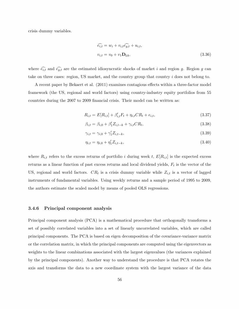
crisis dummy variables.
ei,t = wi + vi,teg,t + ui,t,
vi,t = v0 + v1Di,t, (3.36)
where ei,t and eg,t are the estimated idiosyncratic shocks of market i and region g. Region g can
take on three cases: region, US market, and the country group that country i does not belong to.
A recent paper by Bekaert et al. (2011) examines contagious effects within a three-factor model
framework (the US, regional and world factors) using country-industry equity portfolios from 55
countries during the 2007 to 2009 financial crisis. Their model can be written as:
Ri,t = E[Ri,t] + β′i,tFt + ηi,tCRt + ei,t, (3.37)
βi,t = βi,0 + β′1Zi,t−k + γi,tCRt, (3.38)
γi,t = γi,0 + γ′1Zi,t−k, (3.39)
ηi,t = ηi,0 + η′1Zi,t−k, (3.40)
where Ri,t refers to the excess returns of portfolio i during week t, E[Ri,t] is the expected excess
returns as a linear function of past excess returns and local dividend yields, Ft is the vector of the
US, regional and world factors. CRt is a crisis dummy variable while Zi,t is a vector of lagged
instruments of fundamental variables. Using weekly returns and a sample period of 1995 to 2009,
the authors estimate the scaled model by means of pooled OLS regressions.
3.4.6 Principal component analysis
Principal component analysis (PCA) is a mathematical procedure that orthogonally transforms a
set of possibly correlated variables into a set of linearly uncorrelated variables, which are called
principal components. The PCA is based on eigen decomposition of the covariance-variance matrix
or the correlation matrix, in which the principal components are computed using the eigenvectors as
weights to the linear combinations associated with the largest eigenvalues (the variances explained
by the principal components). Another way to understand the procedure is that PCA rotates the
axis and transforms the data to a new coordinate system with the largest variance of the data
56

projection lying on the first coordinate (the first principal component), and the second largest
variance on the second coordinate, and so on. Conceptually, the PCA allows researchers to extract
common latent factors from a high-dimensional data set and to focus on the variables that explain
the most variations in the underlying data (dimension reduction).
Calvo and Reinhart (1995) study the weekly return comovements between the Asian and Latin
American emerging market stock markets during the Mexican crisis. The authors argue that the
first principal component relates closely to the common external fundamentals and document ap-
parent increases in the explanatory power of the first component during February 1994 to December
1994. They also document substantial increases in explanatory power in the second principal com-
ponent, which they refer to as some ‘Mexico’ crisis effects, most notably in Latin America. Kamin-
sky and Reinhart (2001) study the daily returns of four types of asset markets in 35 developed
and developing economies during 1997 to 1999 and find that South Korea, Malaysia, Turkey and
Greece have the lowest market comovements with other economies in their respective regions. For
the G7 economies, the authors document strong evidence of comovements between the UK, France,
Germany and Italy, and between the US and Canada, while the comovements between Japan with
the rest of the G7 countries were the lowest. Eichengreen et al. (2009) use PCA to examine the
common factors that drove the CDS spreads of major banks and find increasing importance in
these factors during the subprime crisis. These factors are found to be associated with heightening
credit risks within the US banking industry.
In the next section I will summarise the major empirical findings of the methodologies that
have been reviewed above.
3.5 Summary of empirical evidence
3.5.1 Probit and logit models and leading indicators studies
Eichengreen et al. (1996) test for contagion conditional on currency crises using a sample comprising
of quarterly data from 20 industrial countries during the period between 1959 and 1993. Within a
probit regression framework, their empirical results reject the hypothesis of no contagion, so that
the occurrence of a currency crisis in one country increases the probability of a speculative attack
in the domestic currency of other countries by approximately eight per cent. In the second part of
57

their analysis, they replace the crisis dummy variable with some weighted variables according to two
weighting schemes. The two weighting schemes relate to the extent and intensities of trade linkages
and the similarities of macroeconomic variables between the shocked and unaffected countries.
Their results lend support to currency contagion being transmitted via trade linkages rather than
macroeconomic similarities.
Caramazza et al. (2000) use panel probit models with monthly data for 61 industrial and devel-
oping countries over the period between 1990 and 1998 to examine the roles of external and internal
(macroeconomic) imbalances, financial weaknesses (reserve adequacy), trade and financial linkages
(channels for contagion), and institutional factors (exchange rate regimes and capital controls) in
explaining the spillover effects during the Mexican devaluation in 1994, the East Asian Crisis in
1997, and the Russian defaults on bonds in 1998. The empirical results show that indicators of
financial linkages and weaknesses are significant in explaining the crisis effects while weak output
growth has a larger role than external imbalances in reducing the probability of the occurrence of
a crisis. In addition, spillovers via trade linkages have a larger role for countries with weak current
account balances while the exchange rate and capital control regimes are found to be irrelevant in
explaining the occurrence of a crisis.
Kaminsky (1999) uses monthly data of 102 financial crises from 20 developing countries during
the period between 1970 and 1997 to investigate the causes of crises and examine the validity
of some indicators in forecasting financial crises. The results show that crises develop alongside
multiple economic problems. The author aggregated individual indicators of currency and banking
crises into four composite indicators and tested their abilities to predict crises (out-of-sample), and
found that the probability of a currency crisis had increased for Thailand, the Philippines and
Malaysia over the period between 1996 and 1997. The overall findings suggest that composite
leading indicators bear some degree of predictability over the occurrence of crisis events. Hardy
and Pazarbasioglu (1998) use a sample of 50 developing countries from 1976 to 1997 to examine
the predictability of a set of macroeconomic indicators over the occurrence of crises. The results
show that real GDP growth, domestic inflation, credit expansion, capital inflows, real interest rates
and real effective exchange rates are significant predictors.
58
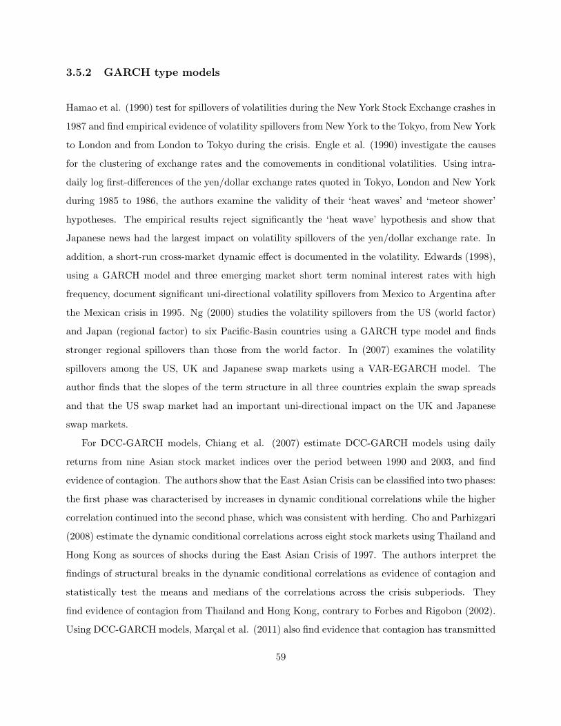
3.5.2 GARCH type models
Hamao et al. (1990) test for spillovers of volatilities during the New York Stock Exchange crashes in
1987 and find empirical evidence of volatility spillovers from New York to the Tokyo, from New York
to London and from London to Tokyo during the crisis. Engle et al. (1990) investigate the causes
for the clustering of exchange rates and the comovements in conditional volatilities. Using intra-
daily log first-differences of the yen/dollar exchange rates quoted in Tokyo, London and New York
during 1985 to 1986, the authors examine the validity of their ‘heat waves’ and ‘meteor shower’
hypotheses. The empirical results reject significantly the ‘heat wave’ hypothesis and show that
Japanese news had the largest impact on volatility spillovers of the yen/dollar exchange rate. In
addition, a short-run cross-market dynamic effect is documented in the volatility. Edwards (1998),
using a GARCH model and three emerging market short term nominal interest rates with high
frequency, document significant uni-directional volatility spillovers from Mexico to Argentina after
the Mexican crisis in 1995. Ng (2000) studies the volatility spillovers from the US (world factor)
and Japan (regional factor) to six Pacific-Basin countries using a GARCH type model and finds
stronger regional spillovers than those from the world factor. In (2007) examines the volatility
spillovers among the US, UK and Japanese swap markets using a VAR-EGARCH model. The
author finds that the slopes of the term structure in all three countries explain the swap spreads
and that the US swap market had an important uni-directional impact on the UK and Japanese
swap markets.
For DCC-GARCH models, Chiang et al. (2007) estimate DCC-GARCH models using daily
returns from nine Asian stock market indices over the period between 1990 and 2003, and find
evidence of contagion. The authors show that the East Asian Crisis can be classified into two phases:
the first phase was characterised by increases in dynamic conditional correlations while the higher
correlation continued into the second phase, which was consistent with herding. Cho and Parhizgari
(2008) estimate the dynamic conditional correlations across eight stock markets using Thailand and
Hong Kong as sources of shocks during the East Asian Crisis of 1997. The authors interpret the
findings of structural breaks in the dynamic conditional correlations as evidence of contagion and
statistically test the means and medians of the correlations across the crisis subperiods. They
find evidence of contagion from Thailand and Hong Kong, contrary to Forbes and Rigobon (2002).
Using DCC-GARCH models, Marcal et al. (2011) also find evidence that contagion has transmitted
59
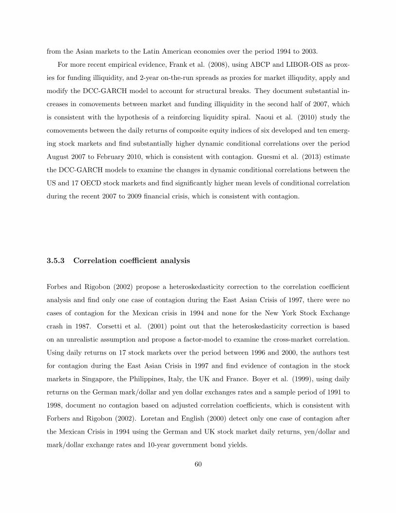
from the Asian markets to the Latin American economies over the period 1994 to 2003.
For more recent empirical evidence, Frank et al. (2008), using ABCP and LIBOR-OIS as prox-
ies for funding illiquidity, and 2-year on-the-run spreads as proxies for market illiqudity, apply and
modify the DCC-GARCH model to account for structural breaks. They document substantial in-
creases in comovements between market and funding illiquidity in the second half of 2007, which
is consistent with the hypothesis of a reinforcing liquidity spiral. Naoui et al. (2010) study the
comovements between the daily returns of composite equity indices of six developed and ten emerg-
ing stock markets and find substantially higher dynamic conditional correlations over the period
August 2007 to February 2010, which is consistent with contagion. Guesmi et al. (2013) estimate
the DCC-GARCH models to examine the changes in dynamic conditional correlations between the
US and 17 OECD stock markets and find significantly higher mean levels of conditional correlation
during the recent 2007 to 2009 financial crisis, which is consistent with contagion.
3.5.3 Correlation coefficient analysis
Forbes and Rigobon (2002) propose a heteroskedasticity correction to the correlation coefficient
analysis and find only one case of contagion during the East Asian Crisis of 1997, there were no
cases of contagion for the Mexican crisis in 1994 and none for the New York Stock Exchange
crash in 1987. Corsetti et al. (2001) point out that the heteroskedasticity correction is based
on an unrealistic assumption and propose a factor-model to examine the cross-market correlation.
Using daily returns on 17 stock markets over the period between 1996 and 2000, the authors test
for contagion during the East Asian Crisis in 1997 and find evidence of contagion in the stock
markets in Singapore, the Philippines, Italy, the UK and France. Boyer et al. (1999), using daily
returns on the German mark/dollar and yen dollar exchanges rates and a sample period of 1991 to
1998, document no contagion based on adjusted correlation coefficients, which is consistent with
Forbers and Rigobon (2002). Loretan and English (2000) detect only one case of contagion after
the Mexican Crisis in 1994 using the German and UK stock market daily returns, yen/dollar and
mark/dollar exchange rates and 10-year government bond yields.
60
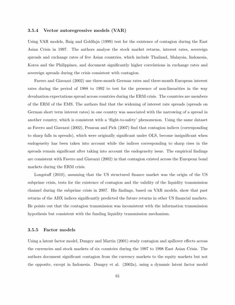
3.5.4 Vector autoregressive models (VAR)
Using VAR models, Baig and Goldfajn (1999) test for the existence of contagion during the East
Asian Crisis in 1997. The authors analyse the stock market returns, interest rates, sovereign
spreads and exchange rates of five Asian countries, which include Thailand, Malaysia, Indonesia,
Korea and the Philippines, and document significantly higher correlations in exchange rates and
sovereign spreads during the crisis consistent with contagion.
Favero and Giavazzi (2002) use three-month German rates and three-month European interest
rates during the period of 1988 to 1992 to test for the presence of non-linearities in the way
devaluation expectations spread across countries during the ERM crisis. The countries are members
of the ERM of the EMS. The authors find that the widening of interest rate spreads (spreads on
German short term interest rates) in one country was associated with the narrowing of a spread in
another country, which is consistent with a ‘flight-to-safety’ phenomenon. Using the same dataset
as Favero and Giavazzi (2002), Pesaran and Pick (2007) find that contagion indices (corresponding
to sharp falls in spreads), which were originally significant under OLS, become insignificant when
endogeneity has been taken into account while the indices corresponding to sharp rises in the
spreads remain significant after taking into account the endogeneity issue. The empirical findings
are consistent with Favero and Giavazzi (2002) in that contagion existed across the European bond
markets during the ERM crisis.
Longstaff (2010), assuming that the US structured finance market was the origin of the US
subprime crisis, tests for the existence of contagion and the validity of the liquidity transmission
channel during the subprime crisis in 2007. His findings, based on VAR models, show that past
returns of the ABX indices significantly predicted the future returns in other US financial markets.
He points out that the contagion transmission was inconsistent with the information transmission
hypothesis but consistent with the funding liquidity transmission mechanism.
3.5.5 Factor models
Using a latent factor model, Dungey and Martin (2001) study contagion and spillover effects across
the currencies and stock markets of six countries during the 1997 to 1998 East Asian Crisis. The
authors document significant contagion from the currency markets to the equity markets but not
the opposite, except in Indonesia. Dungey et al. (2002a), using a dynamic latent factor model
61
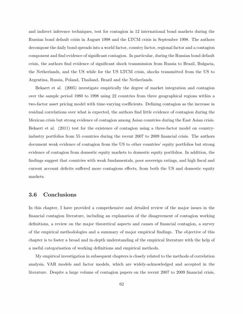
and indirect inference techniques, test for contagion in 12 international bond markets during the
Russian bond default crisis in August 1998 and the LTCM crisis in September 1998. The authors
decompose the daily bond spreads into a world factor, country factor, regional factor and a contagion
component and find evidence of significant contagion. In particular, during the Russian bond default
crisis, the authors find evidence of significant shock transmission from Russia to Brazil, Bulgaria,
the Netherlands, and the US while for the US LTCM crisis, shocks transmitted from the US to
Argentina, Russia, Poland, Thailand, Brazil and the Netherlands.
Bekaert et al. (2005) investigate empirically the degree of market integration and contagion
over the sample period 1980 to 1998 using 22 countries from three geographical regions within a
two-factor asset pricing model with time-varying coefficients. Defining contagion as the increase in
residual correlations over what is expected, the authors find little evidence of contagion during the
Mexican crisis but strong evidence of contagion among Asian countries during the East Asian crisis.
Bekaert et al. (2011) test for the existence of contagion using a three-factor model on country-
industry portfolios from 55 countries during the recent 2007 to 2009 financial crisis. The authors
document weak evidence of contagion from the US to other countries’ equity portfolios but strong
evidence of contagion from domestic equity markets to domestic equity portfolios. In addition, the
findings suggest that countries with weak fundamentals, poor sovereign ratings, and high fiscal and
current account deficits suffered more contagious effects, from both the US and domestic equity
markets.
3.6 Conclusions
In this chapter, I have provided a comprehensive and detailed review of the major issues in the
financial contagion literature, including an explanation of the disagreement of contagion working
definitions, a review on the major theoretical aspects and causes of financial contagion, a survey
of the empirical methodologies and a summary of major empirical findings. The objective of this
chapter is to foster a broad and in-depth understanding of the empirical literature with the help of
a useful categorisation of working definitions and empirical methods.
My empirical investigation in subsequent chapters is closely related to the methods of correlation
analysis, VAR models and factor models, which are widely-acknowledged and accepted in the
literature. Despite a large volume of contagion papers on the recent 2007 to 2009 financial crisis,
62

to my knowledge, this thesis is the first study that comprehensively tests for contagion travelling
from the US structured finance market to the international markets. This is surprising given the
increasing importance and market size of the structured finance market to contagion and financial
stability. I fill this gap by first testing for the existence of contagion and then evaluating the validity
of a few widely-acknowledged contagion transmission channels while taking every necessary step
to ensure the robustness of my findings. In addition, I innovate and test whether there are any
crisis-related factors in relation to the structured finance market that have affected the US equity
market during the subprime and global financial crises.
In the next chapter, I present my first empirical investigation of contagion travelling from the
US structured finance market to the broad equity, financial equity and government bond markets
in the G5 countries.
63

THIS PAGE INTENTIONALLY LEFT BLANK
64
Chapter 4
An Empirical Investigation of
Contagion During the Recent 2007 to
2009 Financial Crisis: Evidence from
the G5 Countries
4.1 Introduction
Longstaff’s (2010) paper is one of the earliest studies to examine contagion during the recent
2007 to 2009 financial crisis. The author documents evidence of significant increases in cross-
market linkages between the less liquid US subprime structured finance market and a number of
domestic US asset markets, which is consistent with the existence of contagion. Longstaff’s (2010)
investigation focuses exclusively on domestic US markets and does not consider international cross-
market spillovers. I will fill this gap and examine contagion travelling from the US structured
finance market to a number of international developed markets.
There are a number of reasons why contagion may have been present across international
markets during the subprime crisis. First, financial institutions that suffered huge write-downs are
in general large in size and are characterised by extensive cross-market functionality. The huge
losses brought by the write-downs of subprime structured finance portfolios in these institutions
65
raised widespread concern about insolvency and possible increases in risk aversion across economies.
Investors, anticipating the spillovers of shocks, may divert their investments away from distressed
sectors to safer markets, leading to increases in market comovements during the crisis. Second, the
realisation of extreme market illiquidity in the US structured finance market may force lenders to
tighten their credit, resulting in a severe funding illiquidity in a number of markets. Market makers
and institutional investors, who faced higher funding costs, were unable to provide sufficient market
liquidity resulting in surging market illiquidity and declines in asset prices (Brunnermeier and
Pedersen, 2009). Third, hedge funds and institutional investors with levered positions were forced
to liquidate assets in unaffected markets to meet margin calls, redemptions and contingent liabilities
as the collateral values of their structured finance portfolios declined.19 All these arguments imply
spillovers of shocks from the US to the international markets during the recent crisis and motivate
my empirical investigation.
This chapter is an empirical investigation of contagion from the US structured finance market
to a number of international equity and government bond markets of the G5 countries during the
subprime and the subsequent global financial crises. The US structured finance market in this
chapter refers specifically to the US subprime RMBS market, which was one of the earliest markets
to collapse during the crisis (Longstaff, 2010) and was tracked by a family of subprime RMBS
benchmark indices - the ABX indices. The G5 countries are developed economies that include the
US, UK, France, Germany and Japan and represent over half the world’s total Gross Domestic
Product (GDP). Following Longstaff (2010), in the first part of this analysis I will formulate my
contagion tests within a VAR model framework and I will seek to detect any significant predictive
power (Granger-causality) in the ABX indices over the international market returns. The main
benefit of using a VAR model is that it enables me to account for possible endogeneity between the
various market variables and focus on inquiring whether the past performance of the ABX indices
explains the contemporaneous returns of the international markets. Furthermore, I will test the
validity of a few widely-acknowledged contagion transmission channels relating to funding illiquidity,
credit risk and trading patterns of financial stocks. In the second part of this analysis, to ensure
the robustness of my findings, I will exploit an alternative method of testing for contagion following
19Allen and Gale (2000) propose a model in which banking institutions may liquidate cross-holdings of depositsacross regions during a crisis to meet funding liquidity requirements, while Kodres and Pritsker (2002) propose amodel within a hedging framework in which shocks propagate through portfolio rebalancing for the purposes ofmacroeconomic risk adjustments.
66
Forbes and Rigobon (2002) and analyse the correlation coefficients between the international market
and the ABX indices to detect any significant increases in unconditional correlations during the
crises.
The remainder of this chapter is organised as follows. Section 2 explains my hypotheses. Section
3 introduces the ABX indices, which are the benchmark indices for the structured finance market.
Section 4 explains my methodological framework and provides details on my data and variable
construction. Section 5 presents and discusses my empirical findings. Section 6 tests the validity
of the contagion transmission channels. Section 7 reports the results of the contagion tests based
on daily frequency data. Section 8 reports additional test results that account for simultaneous
spillovers from various major US markets to the international markets. Section 9 presents the
findings of the correlation coefficient analysis of Forbes and Rigobon (2002) and Section 10 concludes
this chapter.
4.2 Hypotheses
The first part of this analysis aims to identify any significant increases in cross-market linkages by
examining the dependencies between the US structured finance market and a number of interna-
tional equity and government bond markets before, during, and after the crisis. The first hypothesis
can be written as:
H1: There are significant increases in the predictive power of the lagged US structured finance
market index returns (as measured by the ABX indices) for the G5 equity and government
bond market index returns during the subprime and the global financial crises.
Prior to the subprime crisis, the explanatory power of the ABX indices over the international
market returns reflects the level of interdependence between the structured finance market and
the international markets during the tranquil pre-crisis subperiod and is expected to be negligible
prior to the crisis. During the crisis subperiods, as shocks propagate from the structured finance
market to the international markets, I expect to identify substantive increases in the predictive
abilities of the lagged ABX index returns over the international market returns. In addition, a
post-crisis window is included in the analysis to test whether the predictive abilities of the ABX
67
indices persisted after the recent crisis.
On the theoretical side, there are a number of studies that explain how contagion transmits
from one market to another. These studies are of fundamental importance to understanding the
dynamics of shock spillovers. A brief review on the liquidity and risk premia transmission channels
is offered in the following sections.
4.2.1 The liquidity transmission channel
The liquidity transmission channel refers to the mechanism by which an idiosyncratic shock to a
market translates into a subsequent fall in liquidity in other markets. In the literature, liquidity is
defined as funding liquidity (which is the ability to fund any solvent agent to fulfill their immediate
demand for money) and as market liquidity (which refers to the ease by which an asset position can
be sold in financial markets). Recent studies consider market illiquidity as a systematic risk factor
within an asset pricing context (see, for example, Amihud, 2002; Acharya and Pedersen, 2005) and
find significant relations between market illiquidity risk and the cross-section of expected returns.
Previous studies have shown that market illiquidity risk is priced. Consequently, I will review the
market liquidity transmission channel together with the risk premia channel in the next section.
Contagion transmission via funding liquidity refers to a situation where institutional investors
or mutual funds liquidate their holdings to fund their future redemptions and contingent liabilities
during a period of market distress. Levered hedge funds may be obliged to liquidate assets in
unaffected markets to meet margin calls, which leads to higher market comovements during the crisis
(Calvo and Mendoza, 2000; Kodres and Pritsker, 2002; Ben-David et al., 2012). Allen and Gale
(2000) present a model that focuses on the role of the banking system in financial contagion. The
authors argue that financial shocks cause banks to liquidate cross-holding deposits across regions,
leading to severe cross-market funding illiquidity and asset comovements. Similarly, Kaminsky and
Reinhart (2000) point out that banks in tranquil markets may tighten credit lines for prudence
motives and rebalance their overall risk exposure in anticipation of shocks. The main implication
of these studies is that funding illiquidity may induce substantive liquidations and downside price
pressure on financial assets during the crisis. Following Longstaff (2010), I will evaluate the validity
of the funding liquidity channel and test whether the ABX index returns predict the level of trading
intensity in the financial stocks of the G5 countries. A higher level of trading activities in financial
68
stocks during the crisis, as predicted by the ABX index returns, is consistent with possible portfolio
rebalancing by institutional investors due to financial constraints and funding liquidity purposes.
My second hypothesis is formulated as follows:
H2: There were significant increases in the predictive power of US structured finance market
returns for the level of trading intensity in G5 financial stocks relative to the market (as
measured by the trading ratios: the aggregate trading volume in market value of a financial
equity index to the aggregate trading volume in market value of an equity market composite
index) during the subprime crisis.
4.2.2 The risk premia transmission channel
The risk premia transmission channel refers to the comovement of asset prices that occurs as a
result of changes in risk premia after a shock hits a market. For instance, an idiosyncratic shock
to one market leads to subsequent increases in risk premia expected by investors in other markets.
Amihud (2002), and Acharya and Pedersen (2005) document the significant role of aggregate
and idiosyncratic market illiquidity in asset pricing. Their findings show that market illiquidity risk
is priced with considerable time variation and suggest a possible ‘flight-to-liquidity’ phenomenon.
Longstaff (2004) finds significant liquidity premia in the yield spreads between the more liquid
US Treasury bonds over the Refcorp bonds suggestive of some market liquidity component in the
Treasury bond yields. Liu et al. (2006) document significant time-varying liquidity risk premia
in US Treasury bonds between 1988 and 2002. These studies support the notion that investors
have certain liquidity preferences and that the ‘flight-to-safety’ phenomenon may be driven by
market liquidity apart from credit risk considerations. In the context of contagion, shocks might
have been transmitted via changes in market illiquidity risk and translated into subsequent ‘flights’
into more liquid assets and systematic changes in trading patterns. In addition, funding and
market illiquidity might be reinforcing. Brunnermeier and Pedersen (2009) present a model that
establishes the relation between funding and market illiquidity. The authors argue that traders’
funding illiquidity results in higher transaction costs and risks in financing trades that in turn result
in higher market illiquidity and lower asset prices.
One other widely-acknowledged risk premia refers to the credit risk premia that compensates
69
for default and counterparty risks. Vassalou and Xing (2004) empirically show that credit risk is
systematically priced and explains the cross-section of expected returns. Eichengreen et al. (2009)
study the common factors that have driven the CDS spreads of major banks and document the
increasing importance in these factors during the subprime crisis. In particular, these common
factors are associated with the heightening default risks of the US banking industry. The evidence
of these studies reveals possible time variations in the price of credit risk in the US equity market
and in the financial sector. The credit risk premia may have heightened significantly during the
crisis, leading to substantial portfolio rebalancing and possible ‘flight-to-safety’ from the less risky
assets to the safer and more liquid assets. This chapter evaluates the validity of the risk premia
transmission channel by testing the following hypothesis:
H3: The level of credit risk and market illiquidity risk were significantly predicted by the ABX
index returns during the subprime crisis.
I expect substantive increases in the predictive ability of the ABX index returns over the level of
credit risk and market illiquidity risk (as measured by the interest rate swap spreads (IRSS)) during
the crisis and shall interpret these increases as evidence of contagion via the risk premia channel.
4.2.3 The ‘flight-to-safety’ phenomenon
In the literature, several empirical studies have examined the ‘flight-to-safety’ phenomenon in which
investors switch from equity to other asset classes during a crisis to reduce their risk exposure (see,
for example, Goeij and Marquering, 2004; Baur and Lucey, 2009). Despite the fact that both
directions of flights between stocks and government bonds have been identified empirically, the
‘flight-to-safety’ phenomenon is consistent with the risk premia channel in that an increase in the
required risk premia or risk aversion in a stock market (for instance, as a result of market illiquidity
or shifts in expectations) may induce investors to pursue safer fixed-income investments. In this
study, I will test whether the comovements between the weekly returns of the domestic equity and
government bond market indices might be predicted by the ABX index returns to reveal the extent
of the impact of the structured finance market on the degree of ‘flight-to-safety’ in the G5 countries.
Hence, my hypothesis is written as follows:
70
H4: The conditional correlations (between the returns of domestic equity and government bond
indices) were predicted by the ABX index returns during the subprime crisis.
In the next section, I will introduce the benchmark indices for the structured finance market,
the ABX indices, and report summary statistics.
4.3 The ABX indices
Following Longstaff (2010), the ABX indices are used to track the performance of the US structured
finance market. The ABX indices are equally-weighted and static portfolios that reference 20
subprime RMBS transactions. Every six months, the ABX indices are reconstituted with new
on-the-run index vintages, each referencing 20 new subprime RMBS deals that have been issued
during the six months prior to index initiation. There are five sub-indices within the ABX family
that correspond to the AAA, AA, A, BBB and BBB- credit ratings of the underlying RMBS deals.
The ABX.HE.06-1 series is the first vintage followed by the ABX.HE.06-2 series, which was formed
in July 2006, while the ABX.HE.07-1 and ABX.HE.07-2 indices were issued in January and July
2007, respectively. The subprime RMBS issuance declined dramatically during the crisis and no
more ABX indices were issued. The ABX.HE.07-2 index remained the on-the-run ABX index up
to the end of my sample period.20
Throughout this chapter, I will obtain the ABX indices from Reuters and consistently use
the daily and weekly lagged returns (based on quotes on Wednesdays) of the ABX.HE.06-1 index
vintage (the first vintage of the ABX index) as exogenous variables in my empirical model. Reuters
is used because it is the longest vintage series available within the ABX family and covers the entire
subprime and global crises. Fig. 4-1 plots the price levels of the five ABX subindices belonging to
the ABX.HE.06-1 vintage from January 2006 to December 2011. All five indices were, in general,
close to their par value of $100 in 2006 and started to decline sharply in early 2007. In particular,
the three lowest-rated indices fell dramatically from 2007Q2 onwards and tumbled during the first
half of 2009. The three highest-rated ABX indices largely started to recover, most remarkably in
the ABX AAA and AA indices, from the second half of 2009 onwards. Throughout the rest of the
sample period, the ABX AAA index remained largely free of significant shocks while both the ABX
20The ABX PENAAA indices, which reference AAA-rated bonds that are second to last in principal distributionpriority, were introduced in May 2008.
71
AA and A indices started to decline again at the start of year 2011. Fig. 4-2 plots the log first
differences (continuous returns) of the ABX indices over my sample period. Again, I observe largely
no shocks in the ABX indices during 2006 and substantively higher volatilities from 2007 onwards,
which was during the subprime crisis subperiod. In addition, the ABX index returns exhibited
considerable correlation and skewness during the crisis subperiods. The high volatilities persisted
throughout 2007 and 2008, with occasional negative spikes in returns. The three highest-rated ABX
indices started to recover from mid-2009, as shown by the clustered positive spikes of returns. The
volatilities of the ABX indices remained largely lower in 2010 and started to rise again moderately
from mid-2011 onwards.
Table 4.1 reports the descriptive statistics of the log first differences of the ABX indices. During
the pre-crisis subperiod, the mean returns are all positive among the five ABX indices and have be-
come negative during the subprime crisis, global crisis and post-crisis subperiods while the negative
mean returns were the largest in the BBB and BBB- indices. The standard deviations of all ABX
indices are remarkably higher during and after the crises. Throughout the entire sample period,
the correlation between the weekly returns of the ABX AAA and AA indices is considerable while
the cross-correlations between the A, BBB and BBB- indices are high.
There are a few precautions with regard to the use of the returns of the ABX.HE.06-1 indices
as exogenous variables in my analysis. First, each ABX vintage is in fact only a small subset of
the universe of subprime RMBS and ABS products and, therefore, is inevitably limited in market
coverage. In addition, for each referenced MBS deal, only part of the capital structure is referenced
by the five tranches of the ABX indices (see Fender and Scheicher, 2009). In particular, the ABX
AAA index does not reference the most senior tranche of the MBS deals, such that the ABX prices
reflect higher durations than those remaining AAA-rated subprime RMBSs (Fender and Hordahl,
2008). Nonetheless, Fender and Hordahl (2008) note that the bias with regard to the insufficient
market coverage may not be significant as the RMBS deals referenced by the ABX indices are
likely to be similar with the remaining subprime RMBSs in collateral and loan-to-value ratios,
suggesting that the ABX HE.06-1 vintage represents a reasonably satisfactory benchmark for the
US structured finance market.
72
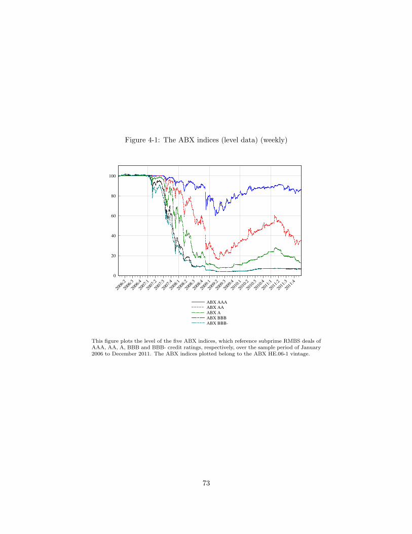
Figure 4-1: The ABX indices (level data) (weekly)
0
20
40
60
80
100
2006:2
2006:3
2006:4
2007:1
2007:2
2007:3
2007:4
2008:1
2008:2
2008:3
2008:4
2009:1
2009:2
2009:3
2009:4
2010:1
2010:2
2010:3
2010:4
2011:1
2011:2
2011:3
2011:4
ABX AAA
ABX AA
ABX A
ABX BBB
ABX BBB-
This figure plots the level of the five ABX indices, which reference subprime RMBS deals ofAAA, AA, A, BBB and BBB- credit ratings, respectively, over the sample period of January2006 to December 2011. The ABX indices plotted belong to the ABX HE.06-1 vintage.
73
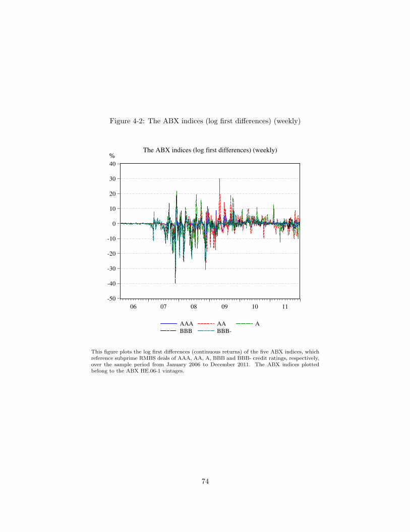
Figure 4-2: The ABX indices (log first differences) (weekly)
-50
-40
-30
-20
-10
0
10
20
30
40
06 07 08 09 10 11
AAA AA A
BBB BBB-
%The ABX indices (log first differences) (weekly)
This figure plots the log first differences (continuous returns) of the five ABX indices, whichreference subprime RMBS deals of AAA, AA, A, BBB and BBB- credit ratings, respectively,over the sample period from January 2006 to December 2011. The ABX indices plottedbelong to the ABX HE.06-1 vintages.
74
4.4 Methodologies
This chapter adopts a vector autoregressive (VAR) model framework with exogenous variables to
test for contagion from the US structured finance market to the G5 international markets during
the subprime and global crisis. VAR models have been widely used in the literature to study the
cross-market spillovers of shocks during crisis (see, for example, Baig and Goldfajn, 1999; Nagayasu,
2001; Favero and Giavazzi, 2002; Forbes and Rigobon, 2002; Pesaran and Pick, 2007; Longstaff,
2010).21
Using weekly returns of the domestic equity and government bond indices that are modelled
within a system of equations for each country, I am able to account for any potential endogeneity
between the markets and test for any significant predictive power in the ABX index returns over the
international market returns. Any increases in predictive power (Granger-causality) of the ABX
index returns over the international market returns during the crisis are reasonably interpreted
as evidence of contagion from the US structured finance market to the international markets. To
capture the dynamic effects of shock propagation, a lag length of four (equivalent to a month) has
been selected for the VAR models.22 Since the structured finance market was primarily driven by
the US housing and the subprime credit markets that were relatively exogenous to the US and the
international stock and government bond markets, I follow Longstaff (2010) and assert that the
ABX index returns are strictly exogenous in the VAR model.23 The VAR(4) models can be written
in the following reduced form with n endogenous variables:
yt = α0 +
4∑s=1
βsyt−s +
4∑s=1
ϕsABXt−s + ϵt, (4.1)
where yt is a n× 1 vector of endogenous dependent variables (market returns), ABXt−s is the sth
lagged value of the ABX index assumed exogenous to the VAR system, βs is a n × n matrix of
coefficients in the systems of equations, ϕs is a n× 1 vector of coefficients of the lagged ABX index
21Forbes and Rigobon (2002) utilise VAR models to estimate the cross-market correlations between the returns ofthe shocked market and other markets during the crisis subperiod and the full sample. The authors adjust the cross-market conditional correlations estimated for heteroscedasticity and document little evidence of contagion during the1997 East Asian crisis, the 1994 Mexican Peso crisis and the 1987 US stock market crash.
22I have also experimented with other lag orders and obtained qualitatively similar results to those associated withthe four-lag order structure.
23Relaxing this assumption and treating the ABX index returns as an endogenous variable does not change theinterpretation of the findings since the purpose of this analysis is to identify contagion specifically transmitted fromthe structured finance market to the international markets in an uni-directional manner.
75

returns, and ϵt is a n× 1 vector of innovations that are uncorrelated with their own lagged values
and all right-hand side variables.
Since I have five ABX indices for my analysis, five VAR models are estimated and reported
for each subperiod; that is, 20 VAR models estimated over the four subperiods in each country.
Within each country’s VAR model, I will include weekly returns of the composite equity market, the
financial equity, and the government bond indices of the subject country as endogenous variables. I
will also include a latent variable in my VAR models that captures the variations of the composite
equity markets in the remaining four G5 countries using principal component analysis (PCA).
4.4.1 Data and crisis subperiods
Table 4.2 summarises and describes my data set. My data are collected from Datastream and
are based on weekly Wednesday-to-Wednesday returns of the G5 international market indices to
avoid any potential calendar day bias and abnormal trading patterns. The G5 countries include
the US, UK, France, Germany and Japan and represent the five largest global economies. My
sample includes observations between 25 January 2006 and 28 December 2011, and covers the
entire subprime crisis and subsequent global financial crisis.
Consistent with the contagion literature, I will split the sample period into four subperiods, as
discussed in Chapter 2. There are no exact dates that best define the crisis outbreak and, hence,
the definition of crisis subperiods contains a certain degree of subjectivity. Despite that, the criteria
of subperiod selection is based on historical events and market performance. Following Longstaff
(2010), I will define the year 2006 (49 obs) as the pre-crisis subperiod, which is characterised by no
significant shocks in the US structured finance and the international markets, and I will define the
year 2007 (51 obs) as the subprime crisis subperiod, during which the US structured finance market
started to decline sharply. As the crisis went global and was characterised by numerous corporate
bankruptcies and bailouts, the period of 2008Q1 to 2009Q1 (i.e. from 2 January 2008 to 25 March
2009, 65 obs) is defined as the global crisis subperiod. Lastly, I will include a post-crisis window
with data observations between 2 September 2009 and 28 December 2011 (122 observations) to
facilitate comparison across the subperiods. The observations between April 2009 and August 2009
are omitted from the sample because the ABX BBB and BBB- indices were considerably stale, thus
creating near singularity problems in regressions when using daily returns in subsequent sections.
76
4.4.2 Endogenous variables
The endogenous variables used in this study can be written as y(i)t = [EQ
(i)t , FEQ
(i)t , GOV
(i)t , PCA
(i)t ]′
where i refers to the ith country in the G5 countries. The variables EQ, FEQ and GOV denote
the weekly returns of the international market composite, financial equity, and government bond
indices of the G5 countries while the variable PCA are the factor scores (the first principal compo-
nent) from the PCA that capture the variations in the remaining four international equity market
composite index returns. For the underlying data series, I will use the FTSE Global Government
10+ year bond clean price indices for government bond markets, the domestic composite equity
indices for the broad equity markets, and the Datastream-calculated financial price indices for the
performance of the financial equity markets.
Table 4.3 reports the full sample and subsample means and standard deviations of the en-
dogenous variables used in my analysis. Panels A to C report the summary statistics of the weekly
returns of the equity market composite, financial equity, and government bond indices, respectively.
The full sample statistics show that the financial equity indices have the lowest mean returns and
the highest volatilities while the government bond indices have the highest average weekly returns
with the lowest standard deviations. The subsample statistics show that, during the pre-crisis sub-
period, the composite equity and the financial equity indices were largely free of significant shocks
while the government bond markets underperformed. The financial stocks of the G5 countries
largely started to fall during the subprime crisis and declined dramatically during the global crisis
subperiod with high volatilities. The equity market composite indices remained largely stable dur-
ing the subprime crisis and have had negative average returns and considerable volatilities during
the global crisis. In addition, the international government bond markets outperformed their equity
counterparts during the global crisis subperiod, which is consistent with possible ‘flight-to-safety’.
During the post-crisis subperiod, I can observe no obvious patterns in the indices while largely all
markets yielded positive mean returns with high volatilities.
4.4.3 Latent variables - principal component analysis
From an international market perspective, shocks might have transmitted in multiple directions and
sequentially; that is, from the US structured finance market to the US domestic markets and then
to the international markets. To this end, I will use PCA to extract the latent principal components
77
that underlie the overall variation in the international equity markets. The factor scores of the first
principal component extracted are then included as endogenous variables in each VAR model to
control for possible spillovers of shocks from the international markets to the subject market.
For each country, I include the weekly returns of the remaining four countries’ equity market
composite indices as inputs to the PCA and use the factor scores of the first principal component
as endogenous variables in my analysis. For instance, the principal component variable for the
US VAR model is computed by using the returns of the market composite indices of the UK,
France, Germany and Japan as inputs to the PCA. Kaiser’s significance rule is used to determine
the number of significant principal components such that any components with eigenvalues greater
than one are statistically significant and retained. Table 4.4 presents the eigenvalues of the PCA
and the percentage of variance explained by the first principal component for each country. Only
one principal component has been identified and retained for each country. The first principal
components of the G5 countries explain more than 80 per cent of the variance of the equity market
returns in each market. The communalities measure the proportion of each variable’s variance
explained by the principal components. The statistics show that the principal components explain
the variance of the European market returns reasonably well and less satisfactorily for the Japanese
market.
4.5 Empirical findings
I report the country VAR(4) model results for the G5 countries in Tables 4.5 - 4.9, grouped by the
crisis subperiods. I report the sums of factor loadings on the lagged ABX index returns and the R2
for each of the VAR models. The F-tests place restrictions on the ABX factor loadings and test the
null hypothesis that h0 : ϕ(i)j,1 = ϕ
(i)j,2 = ϕ
(i)j,3 = ϕ
(i)j,4 = 0, where j refers to the jth endogenous variables
of the ith country VAR model. Significant F-statistics suggest that at least one of the lagged ABX
index returns significantly predict (Granger-causality) the contemporaneous international market
returns, which is consistent with my definition of contagion.
4.5.1 The pre-crisis subperiod
As shown in my summary statistics, 2006 was largely free from significant shocks and high volatil-
ities. All international equity markets showed signs of stability and growth during this subperiod.
78
The findings of this one-year pre-crisis window reveal the degree of interdependencies between the
US structured finance and the international markets during tranquil market conditions.
These results are in line with my expectation of finding little evidence of predictive power in
the lagged ABX index returns over the international market returns. The cross-market linkages
between the structured finance market and the international markets were in general weak prior to
the subprime crisis. The weak relation documented is reasonable because the structured finance
market was not widely known before the outbreak of the subprime crisis, and the structured finance
securities were in general complex and nontransparent. It was essentially difficult to predict ex ante
the scope and severity of the negative consequences if these securities went insolvent. These results
are consistent with those of Longstaff (2010), who finds little interdependence between the ABX
indices and the other US domestic markets in 2006.
4.5.2 The subprime crisis subperiod
The subprime crisis subperiod contains all of the observations in year 2007 and is characterised
by an increasing threat of subprime mortgage delinquencies and several waves of write-downs in
relation to the troubled subprime ABS portfolios among numerous financial institutions. Both the
equity market composite and financial equity indices in the G5 countries started to fall sharply in
mid-2007.
In the US VAR models, I find strong evidence of contagion from the ABX indices to the US
equity and government bond markets, as evinced by the highly significant F-statistics across the
ABX index variants. First, the results show that the declines in the ABX indices translated into
subsequent higher US government bond market returns, which is consistent with possible ‘flight-
to-safety’ from equity into safer US Treasury bonds during the crisis. In addition, I find significant
F-statistics in the three lowest-rated ABX models in explaining the US S&P500 composite index
returns. As for the financial equity sector, the lagged returns of all ABX indices, except the ABX
AAA index, are highly significant in predicting US financial index returns. In addition, I document
significant findings in the ABX AA, A and BBB models in explaining the principal component
variable.
Next, I will focus on the results of the international country VAR models. My results are in
general significant and consistent with my expectation that the past performance of the ABX indices
79
explain significantly the international equity and government bond market returns. In particular,
I document significant predictive power in largely all the ABX indices (with a positive impact)
over the composite equity and financial index returns in the G5 countries except in the ABX BBB-
models for the UK and German financial indices, and in the AAA model for the Japanese financial
index. I also find that the international government bond index returns are significantly predicted
(with negative sums of ABX factor loadings) by the lagged ABX index returns across all of the
ABX models. Negative shocks in the ABX indices translated into subsequent increases in the
international government bond markets and declines in the international equity markets, which is
consistent with the existence of flights between domestic equity and government bonds. The R2
in the VAR models of the financial indices and the government bond indices consistently increased
compared to those of the pre-crisis subperiod, suggesting higher explanatory power and better
model fit.
4.5.3 The global crisis subperiod
The global crisis subperiod includes the 65 observations between January 2008 and March 2009
and is characterised by the financial institutions’ continual losses in relation to their subprime
mortgage related businesses, severe funding and market illiquidity, and the international stock
market crashes after the Lehman Brothers’ collapse in September 2008. The international equity
markets performed poorly throughout 2008 and plunged in 2009Q1.
The results of the US VAR models are largely insignificant and the R2 are in general lower. The
predictive power of the ABX indices largely disappeared, as evinced by the insignificant F-statistics.
Consistent with the findings of Longstaff (2010), the spillovers of shocks from the US structured
finance market to other domestic US markets have become remarkably weaker in this subperiod.
The international evidence is qualitatively similar to those of the US VAR models in that most
of the predictive power in the lagged ABX index returns vanished, except for a few markets. The
exceptions include the significant results in the financial indices (with negative impact) and in the
three highest-rated ABX models of the government bond markets (with negative impact) in the G5
countries. The empirical findings reveal that the predictive power of the ABX indices has become
weaker and that the international markets were, to a lesser extent, subjected to the shocks from the
US structured finance market during the global financial crisis phase. Nonetheless, I still document
80
evidence of possible ‘flight-to-safety’ from domestic equity into government bonds, as shown by the
significant and negative sums of factor loadings in the government bond market VAR functions.
4.5.4 The post-crisis subperiod
The post-crisis subperiod starts from September 2009 to December 2011 and consists of 123 weekly
observations. It partly covers the ongoing crisis in relation to the troubles of European sovereign
debt markets. Although the European sovereign debt crisis is not the focus of this investigation, I
will include this window to facilitate comparison across the crisis subperiods and to test whether
there was still evidence of contagion from the structured finance market to the international markets
after the global financial crisis.
In the US VAR models, I find marginally significant predictive power (with negative impact) in
the two lowest-rated ABX indices over the US equity market composite and financial index returns.
In addition, I find some evidence of predictive power in the ABX AAA model (with negative impact)
over the government bond index returns. Overall, the findings are less significant than those in the
global crisis subperiod, which is consistent with my expectation of no contagion.
The international evidence is again similar to those of the US VAR models and is in general
insignificant, particularly when referring to the French, German and Japanese VAR models. Despite
the significant F-statistics in a few UK and French VAR models, the predictive power of the ABX
indices has become largely non-existent after the global financial crisis.
4.5.5 Discussions
My empirical findings provide reasonably strong evidence of contagion travelling from the US struc-
tured finance market to all G5 equity markets during the subprime crisis. Financial stocks were,
to a larger extent, subject to the spillovers of shocks from the US structured finance market, which
is consistent with the fact that numerous financial institutions have suffered substantial insolvency
risks as a result of the huge losses they suffered in relation to their subprime ABS portfolios during
the subprime crisis. In addition, the financial institutions’ funding shortage and financial constraints
might have reinforced market illiquidity, which in turn translated into heightened risk aversion and
declines in prices in the international markets (see Brunnermeier and Pedersen, 2009). Another
transmission mechanism relates to investors’ obligated liquidation of cross-market investments in
81

meeting funding requirements and to the subsequent higher selling pressures in foreign asset mar-
kets (for the role of hedge funds during the recent crisis, see Boyson et al. (2010) and Ben-David
et al. (2012)).
I have also documented strong US and international evidence of ‘flight-to-safety’ from equity
into government bonds, as evinced by the significant positive and negative sums of ABX factor
loadings in the lagged returns of the equity and government bond indices, respectively. Facing
higher systematic insolvency risks and trading costs, investors might switch from equity into safer
and more liquid government bonds, which in effect increased the prices of the government bonds
and pushed the stock prices down. ‘Flight-to-safety’ might be motivated from a market liquidity
consideration in that investors prefer actively traded government bonds to illiquid assets to ensure
that the positions can be liquidated readily so that they can fulfil their funding needs.
4.6 How did contagion transmit during the subprime mortgage
crisis?
Having documented solid evidence of contagion, in the following sections I will evaluate the trans-
mission mechanisms of contagion as it passed from the US structured finance market to the inter-
national markets. I will also seek to reveal the dynamics of ‘flight-to-safety’ between the domestic
equity and government bond markets. To this end, I will use a similar VAR(4) model framework
as in the previous sections, with identical crisis subperiods, to model the relationship between a
number of liquidity, credit risk, conditional correlation variables and the ABX index returns. The
endogenous variables are written as: yt = [RATIO(i), IRSS(i), CORR(i)], where RATIO(i) is the
trading ratio of financial stocks relative to the overall market, IRSS(i) is the IRSS, and CORR(i)
is the estimated conditional correlations between the domestic equity and government bond index
returns of the ith country.
4.6.1 Trading ratios
Following Longstaff (2010), I will compute a trading ratio that measures the intensity of trading
activities in the financial equity market relative to the overall market. The trading ratio is calcu-
lated by dividing the aggregate dollar trading volume of a financial equity index by the aggregate
82
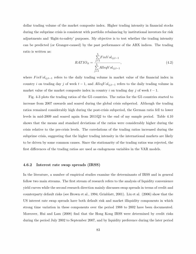
dollar trading volume of the market composite index. Higher trading intensity in financial stocks
during the subprime crisis is consistent with portfolio rebalancing by institutional investors for risk
adjustments and ‘flight-to-safety’ purposes. My objective is to test whether the trading intensity
can be predicted (or Granger-caused) by the past performance of the ABX indices. The trading
ratio is written as:
RATIOit =
5∑j=1
FinV olij,t−1
5∑j=1
AlleqV olij,t−1
, (4.2)
where FinV olij,t−1 refers to the daily trading volume in market value of the financial index in
country i on trading day j of week t − 1, and AlleqV olij,t−1 refers to the daily trading volume in
market value of the market composite index in country i on trading day j of week t− 1.
Fig. 4-3 plots the trading ratios of the G5 countries. The ratios for the G5 countries started to
increase from 2007 onwards and soared during the global crisis subperiod. Although the trading
ratios remained considerably high during the post-crisis subperiod, the German ratio fell to lower
levels in mid-2009 and soared again from 2011Q2 to the end of my sample period. Table 4.10
shows that the means and standard deviations of the ratios were considerably higher during the
crisis relative to the pre-crisis levels. The correlations of the trading ratios increased during the
subprime crisis, suggesting that the higher trading intensity in the international markets are likely
to be driven by some common causes. Since the stationarity of the trading ratios was rejected, the
first differences of the trading ratios are used as endogenous variables in the VAR models.
4.6.2 Interest rate swap spreads (IRSS)
In the literature, a number of empirical studies examine the determinants of IRSS and in general
follow two main streams. The first stream of research refers to the analysis of liquidity convenience
yield curves while the second research direction mainly discusses swap spreads in terms of credit and
counterparty default risks (see Brown et al., 1994; Grinblatt, 2001). Liu et al. (2006) show that the
US interest rate swap spreads have both default risk and market illiquidity components in which
strong time variation in these components over the period 1988 to 2002 have been documented.
Moreover, Hui and Lam (2008) find that the Hong Kong IRSS were determined by credit risks
during the period July 2002 to September 2007, and by liquidity preference during the later period
83
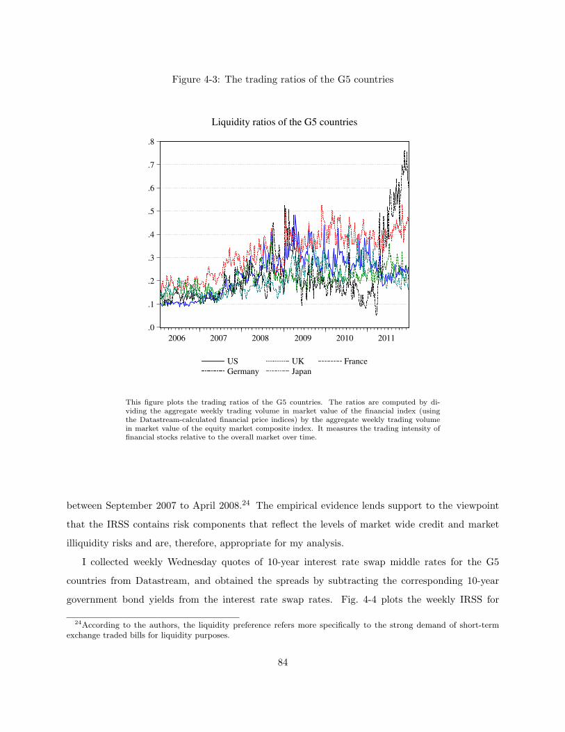
Figure 4-3: The trading ratios of the G5 countries
.0
.1
.2
.3
.4
.5
.6
.7
.8
2006 2007 2008 2009 2010 2011
US UK France
Germany Japan
Liquidity ratios of the G5 countries
This figure plots the trading ratios of the G5 countries. The ratios are computed by di-viding the aggregate weekly trading volume in market value of the financial index (usingthe Datastream-calculated financial price indices) by the aggregate weekly trading volumein market value of the equity market composite index. It measures the trading intensity offinancial stocks relative to the overall market over time.
between September 2007 to April 2008.24 The empirical evidence lends support to the viewpoint
that the IRSS contains risk components that reflect the levels of market wide credit and market
illiquidity risks and are, therefore, appropriate for my analysis.
I collected weekly Wednesday quotes of 10-year interest rate swap middle rates for the G5
countries from Datastream, and obtained the spreads by subtracting the corresponding 10-year
government bond yields from the interest rate swap rates. Fig. 4-4 plots the weekly IRSS for
24According to the authors, the liquidity preference refers more specifically to the strong demand of short-termexchange traded bills for liquidity purposes.
84
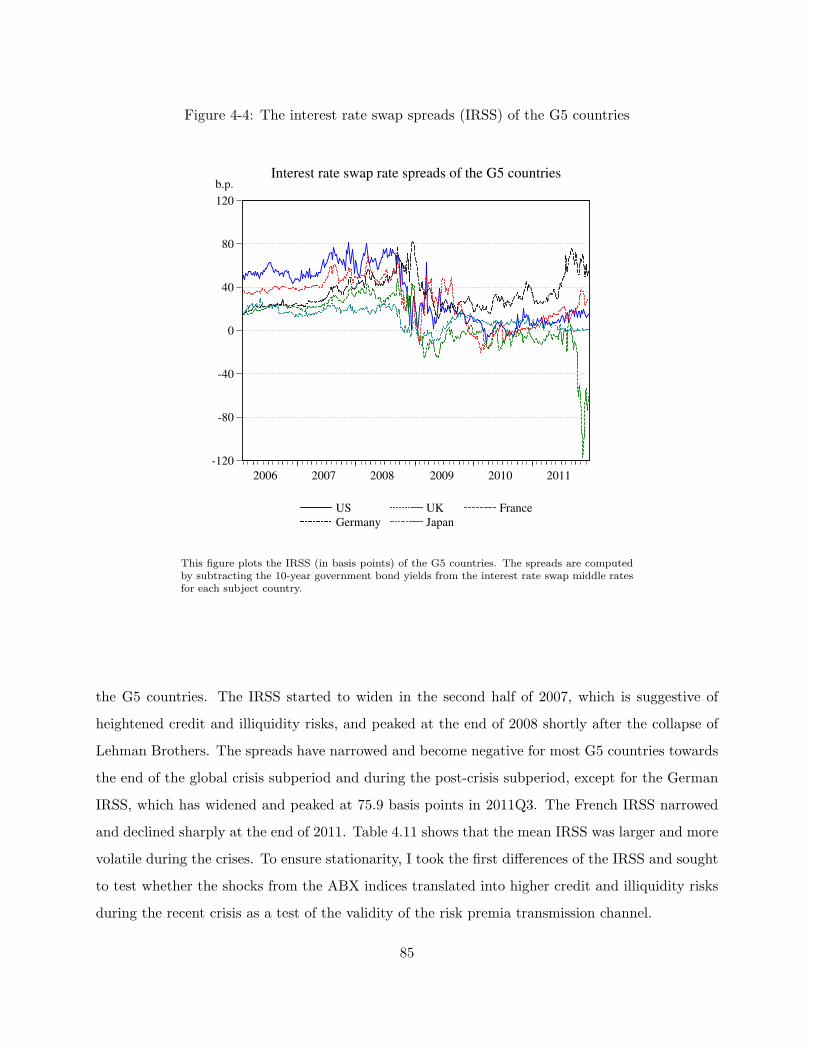
Figure 4-4: The interest rate swap spreads (IRSS) of the G5 countries
-120
-80
-40
0
40
80
120
2006 2007 2008 2009 2010 2011
US UK France
Germany Japan
Interest rate swap rate spreads of the G5 countriesb.p.
This figure plots the IRSS (in basis points) of the G5 countries. The spreads are computedby subtracting the 10-year government bond yields from the interest rate swap middle ratesfor each subject country.
the G5 countries. The IRSS started to widen in the second half of 2007, which is suggestive of
heightened credit and illiquidity risks, and peaked at the end of 2008 shortly after the collapse of
Lehman Brothers. The spreads have narrowed and become negative for most G5 countries towards
the end of the global crisis subperiod and during the post-crisis subperiod, except for the German
IRSS, which has widened and peaked at 75.9 basis points in 2011Q3. The French IRSS narrowed
and declined sharply at the end of 2011. Table 4.11 shows that the mean IRSS was larger and more
volatile during the crises. To ensure stationarity, I took the first differences of the IRSS and sought
to test whether the shocks from the ABX indices translated into higher credit and illiquidity risks
during the recent crisis as a test of the validity of the risk premia transmission channel.
85

4.6.3 Conditional correlations
In the previous sections, I document strong evidence of ‘flight-to-safety’ in the international markets
during the subprime crisis and the global financial crisis. Following a widely-adopted approach in
the literature (see, for example, De Goeij and Marquering, 2004; Li, 2003; Baur and Lucey, 2009), I
have studied the estimated conditional correlations between the weekly returns of domestic equity
and government bond indices to examine the dynamics of the ‘flight-to-safety’ phenomenon during
the recent financial crisis.
I adopt a MGARCH diagonal VECH model to estimate the dynamics between the returns of
the domestic equity market composite and government bond indices in each G5 country and have
obtained a series of conditional correlations for each pair of returns. I assume a VECH specification
in which the variance-covariance matrix is modelled as in the following autoregressive process:
vech(Ht) = C+Avech(Ξt−1Ξ′t−1) +Bvech(Ht−1)
Ξt|It−1 ∼ N(0,Ht). (4.3)
With the restricted form developed by Bollerslev et al.(1988), matrix A and B are assumed to be
diagonal such that:
Ht =
h11t h12t
h21t h22t
, Ξt =
u1tu2t
, C =
c11
c21
c31
, A =
α11 0 0
0 α22 0
0 0 α33
,
B =
β11 0 0
0 β22 0
0 0 β33
.The conditional variances for my two asset returns in each country follow a GARCH(1,1) formula-
tion, characterised by:
hijt = wij + αijui,t−1uj,t−1 + βijhij,t−1 for i, j = 1, 2. (4.4)
where wij , αij , and βij are parameters to be estimated while ui,t−1 and uj,t−1 refer to the regression
residuals of asset i and j at time t− 1, respectively.
Fig. 4-5 plots the time-varying conditional correlations of the domestic equity and government
86
bond market index returns of the G5 countries estimated using the MGARCH diagonal VECH
model. The conditional correlations of the G5 countries are in general negative during the pre-
crisis subperiod and have become more negative during the subprime crisis subperiod, except
for the Japanese correlations in which strong time variations and positive spikes were present.
Towards the end of year 2008, the conditional correlations became less negative, reflecting a higher
degree of market comovements between the G5 domestic stock and government bond markets.
The correlations largely remained negative after the crisis, except for the occasional spikes in
the Japanese and German series. As shown in Table 4.12, the subsample mean correlations largely
became more negative during the subprime crisis and less negative during the global financial crisis.
The summary statistics suggest possible ‘flight-to-safety’ during the subprime crisis subperiod and
higher market comovements (contagion) between the domestic equity and government bond markets
during the global crisis subperiod. The conditional correlation series are included as endogenous
variables in the VAR models to test whether the lagged ABX index returns have predicted the
changes in comovements between domestic equity and government bond market returns during the
crisis.
4.6.4 Empirical findings: The trading ratios, IRSS and conditional correlations
VAR models
Tables 4.13 - 4.17 present the findings of the VAR(4) models with the trading ratios, IRSS and
conditional correlations as endogenous variables and the lagged ABX index returns as exogenous
regressors. The sums of ABX factor loadings and the R2 of each VAR function are reported. The
F-tests are based on the null hypothesis that the ABX factor loadings are jointly equal to zero:
h0 : ϕ(i)j,1 = ϕ
(i)j,2 = ϕ
(i)j,3 = ϕ
(i)j,4 = 0.
Pre-crisis subperiod
During the pre-crisis subperiod, I find limited predictive power in the ABX indices over changes
of trading ratios, IRSS and conditional correlations, except in the German trading ratios and the
Japanese IRSS and correlation VAR models. Although I document some significant results in the
US conditional correlations and the UK trading ratios and IRSS, my findings show that the lagged
ABX index returns do not explain much of the variations in the changes of trading ratios, IRSS and
87
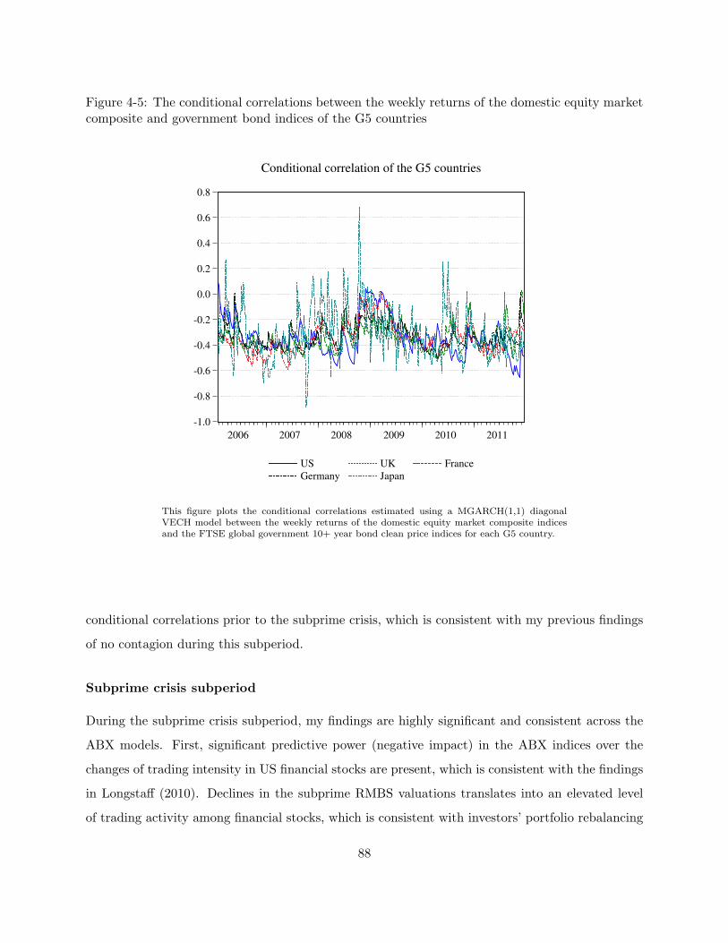
Figure 4-5: The conditional correlations between the weekly returns of the domestic equity marketcomposite and government bond indices of the G5 countries
-1.0
-0.8
-0.6
-0.4
-0.2
0.0
0.2
0.4
0.6
0.8
2006 2007 2008 2009 2010 2011
US UK France
Germany Japan
Conditional correlation of the G5 countries
This figure plots the conditional correlations estimated using a MGARCH(1,1) diagonalVECH model between the weekly returns of the domestic equity market composite indicesand the FTSE global government 10+ year bond clean price indices for each G5 country.
conditional correlations prior to the subprime crisis, which is consistent with my previous findings
of no contagion during this subperiod.
Subprime crisis subperiod
During the subprime crisis subperiod, my findings are highly significant and consistent across the
ABX models. First, significant predictive power (negative impact) in the ABX indices over the
changes of trading intensity in US financial stocks are present, which is consistent with the findings
in Longstaff (2010). Declines in the subprime RMBS valuations translates into an elevated level
of trading activity among financial stocks, which is consistent with investors’ portfolio rebalancing
88

and possible ‘flight-to-safety’. Second, I find significant negative sums of ABX factor loadings in
the three lowest-rated ABX models for the US IRSS. In other words, the widening of the US IRSS
and heightening credit risks during the subprime crisis are predicted by the past performance of
the ABX indices, lending empirical support to the risk premia channel. On the other hand, the
findings of the US conditional correlations are largely insignificant.
The empirical findings for the international market VAR models are remarkably significant,
except in the German correlations and the Japanese trading ratios models. I document significant
negative (positive) relations between the ABX index returns and the changes of trading ratios in
the UK and France (Germany). As for the IRSS, the results are highly significant across the ABX
models and the G5 countries in that shocks from the ABX indices translated into the widening
of IRSS in the G5 countries in weeks. These results suggest that the heightening levels of credit
risk and market illiquidity in the international markets were associated with the shocks from the
structured finance market consistent with contagion transmission via changes in risk premia. In
addition, the conditional correlations were related negatively with the ABX index returns for the
UK, French and Japanese VAR models and positively related with the ABX index returns for the
German ABX AAA and AA models. The declines in the ABX indices during the subprime crisis
subperiod led to increases (decreases) in the changes of correlation in the UK, France and Japan
(Germany). In other words, the ABX shocks led to a higher degree of market comovements (i.e.
contagion) between the domestic equity and government bond markets in the UK, France and
Japan and a higher degree of ‘flight-to-safety’ in the German markets.
Global crisis subperiod
Consistent with my findings in the previous section, my findings of the US VAR models are largely
insignificant, except for the US trading ratios. The higher trading intensity in the US financial
stocks are predicted by the past performance of the US structured finance market during the global
financial crisis. Apart from this, the findings of the US IRSS and conditional correlations are largely
insignificant.
The findings for the international markets are largely insignificant with a few exceptions, such
as: the UK IRSS (negative relation in the ABX AA and A indices), German trading ratios (positive
relation in ABX AA and BBB- indices), and the Japanese IRSS (negative relation in ABX AA and
89
A indices and positive relation in ABX AAA index).
Post-crisis subperiod
In this subperiod, the ABX model results are in general insignificant and the significant predic-
tive power in the ABX indices over the changes in US trading ratios during the global crisis no
longer existed. The R2 are notably lower, which is in line with my expectation of little or limited
explanatory power.
As for the international markets, the predictive power of the ABX indices largely weakened and
became insignificant after the global crisis. The ABX indices no longer contained important market
information that predicted the international market returns during the post-crisis subperiod.
4.6.5 Discussions
In summary, my VAR analysis based on weekly data shows that past returns of the ABX indices
significantly predict (Granger-causality) changes in the trading activities of financial stocks, IRSS
and conditional correlations, especially during the subprime crisis. In particular, the negative shocks
in the ABX indices translated into subsequent higher trading intensity in the domestic financial
stocks in the US, UK, France and lower trading intensity in Germany. The higher trading intensity
in financial stocks is consistent with portfolio rebalancing and ‘fire sales’ of assets due to funding
liquidity constraints and increasing risk aversion.
More remarkably, my findings show that the widening of the G5 IRSS during the subprime crisis
is significantly predicted by the ABX index returns. Taken together with the significant findings
of contagion from the US structured finance market to the international markets in Section 4.5, I
present strong evidence in support of the contagion transmission via increases in credit and market
illiquidity risks. My findings also show that the negative shocks in the ABX indices translated into
subsequent higher comovements between domestic stock and government bond markets in the UK,
France and Japan during the subprime crisis. I find evidence that shocks from the ABX indices
encouraged ‘flight-to-safety’ in the German markets, as evinced by the positive relation between the
lagged ABX index returns and the German conditional correlations. The evidence that the declines
in the ABX indices led to contagion in both the domestic equity and government bond markets is
somewhat contrary to my previous VAR results, in which the negative shocks from the ABX indices
90
translated into lower future stock market and higher government bond market performance.
Nonetheless, my graphical analysis of the conditional correlations and the empirical results (as
shown in Tables 4.5 - 4.9) both lead me to conclude that the ‘flight-to-safety’ between the domestic
and government bond markets existed during the subprime crisis. However, the results in my
liquidity and credit risk VAR models are to be interpreted with caution. First, the fact that the
correlations are first-differenced means that I can only evaluate the relation between the past ABX
index returns and the changes in correlations. The interpretation is limited to testing whether the
past returns of the ABX indices ‘encourage’ or ‘discourage’ the ‘flight-to-safety’ phenomenon. For
instance, assuming that the ABX indices have declined, the ABX factor loadings are negative and
the conditional correlation (level data) was -0.50 at time t− 1, the negative relation dictates that
the decline in the ABX indices translates into a positive change in conditional correlation, say an
increase of 0.10. The conditional correlation at t would become −0.50 + 0.10 = −0.40. In other
words, the ‘flight-to-safety’ may still exist despite the negative relation documented between the
lagged ABX index returns and the changes in conditional correlations. In this sense, I conclude
with caution that the negative shocks from the ABX indices ‘discouraged’ flights in the UK, France
and Japan and ‘encouraged’ flights in the German markets while the ‘flight-to-safety’ phenomenon
was in general present in the G5 countries during the recent crisis.
4.7 Empirical investigation on contagion - daily data
Another widely-acknowledged working definition of contagion focuses on the role of the arrival
of new market information in shock transmission. This definition relates closely to the EMH in
that price discovery of efficient markets is in general immediate and rapid in adjusting to new
market information. Contagion may occur in a fast and immediate manner via the arrival of
information. Engle et al. (1990) show that the volatilities in foreign exchange markets spread
across intra-daily market segments, while Dooley and Hutchison (2009) show empirically that the
US financial and real economic news impacted on the daily changes in emerging markets’ CDS
spreads. Evans (2011) shows that the intra-daily jumps in the US futures market are associated
with US macroeconomic news announcements. Connolly and Wang (2003) show that the market
comovements of the domestic overnight returns in the US, UK and Japanese stock markets are
significantly explained by foreign (US, UK and Japanese) equity market returns, but not by public
91

economic fundamentals. The empirical evidence suggests that contagion may arise in a relatively
fast and immediate manner within trading days.
In the literature, the information contagion transmission channel refers to the mechanism by
which a shocked market signals new market information that affects the asset prices in other mar-
kets. Kaminsky et al. (2003) contend that shocks transmit through the arrival of negative economic
news and immediately affect the collateral values in other markets. King and Wadhwani (1990)
present a rational expectation equilibrium model that explains contagion as the result of market
agents’ attempts to infer equity values based on imperfect information about certain events. Their
model implies that idiosyncratic changes in one market may affect other markets as a result of
information asymmetries and result in the subsequent comovement of market volatilities. Shocks
transmitted via the information transmission mechanism should be ‘fast and furious’ with instan-
taneous adverse market comovement (Kaminsky et al., 2003).
Thus far, my empirical results are consistent with Longstaff (2010) in that the significant pre-
dictive power of the lagged ABX index returns on US and international market returns is identified
over a weekly frequency. I would contend that the significant contagion from the ABX indices
over this frequency is inconsistent with the information transmission mechanism. Nonetheless, the
predictive power of the ABX indices does not rule out the possible existence of short-lived spillovers
of shocks within trading days. I will fill this gap by examining contagion from the ABX indices to
the G5 international markets using daily data frequency.
4.7.1 Methodologies
In this section, I apply the same VAR model framework as in earlier sections and study the de-
pendencies between the ABX indices and the international market indices in the G5 countries. To
detect significant short-lived contagion within one trading week, I use five lags (equivalent to one
trading week) and estimate the following VAR(5) model with n endogenous variables:
yt = α0 +
5∑s=1
βsyt−i +
4∑k=1
5∑s=1
ϕs,kdkABXt−s + ϵt, (4.5)
where yt is a n× 1 vector of endogenous dependent variables (daily returns of the domestic broad
equity, financial equity, and government bond indices, and a daily PCA latent factor variable
92
constructed in the same manner as in Section 4.4.3), βs is an n×n matrix of coefficients, ABXt−s
is the sth lagged ABX index returns, ϕs,k is an n×1 vector of coefficients for the lagged ABX index
returns, dk is a crisis dummy variable denoting the kth crisis subperiod, and ϵt is an n × 1 vector
of innovations that are uncorrelated with their own lagged values and all right-hand side variables.
The main difference between the current VAR model framework and the previous model given
by Equation 4.1 is that I introduce crisis dummy variables and estimate one VAR model for each
country using the full sample period instead of estimating a VAR model separately for each sub-
period. I will then test for the block predictive power (Granger-causality) of the lagged ABX
index returns over the international market returns using standard F-tests of joint significance.
Significant F-statistics suggest that the G5 market returns cannot be explained fully by its own
country-specific factors and that the past idiosyncratic shocks of the ABX indices have a significant
impact on the international market returns observed over subsequent trading days.
4.7.2 Data and summary statistics
My daily data consists of 1385 observations and covers the period between 19 January 2006 and
31 December 2011. The endogenous variables used in the VAR models include the daily returns
of the domestic broad equity, financial equity and government bond indices and the PCA variable
and can be written as yt = [EQ(i)t , FEQ
(i)t , GOV
(i)t , PCA
(i)t ]′.
To account for the time differentials between the international market open and close times, I
follow Forbes and Rigobon (2002) and compute the two-day rolling average returns (or changes)
for each of the variables. In addition, the daily observations between 1 April 2009 and 31 August
2009 are excluded from the current analysis because the ABX indices were considerably stale with
a number of consecutive zero returns that cause near-singularity problems in OLS regressions.
Nevertheless, the main focus of the current investigation is on the subprime and global crisis
subperiods and, hence, the omission of these observations has a limited impact on my main findings.
Crisis dummy variables
Crisis dummy variables denoted by dk, where k = 1,...,4, are introduced to allow changes in
the ABX factor loadings across the crisis subperiods. Unity is assigned to observations within
the specified crisis subperiod, and zero otherwise. While the pre-crisis, subprime and global crisis
93
subperiods are defined with the exact same dates as in earlier analysis, the post-crisis subperiod
starts from 1 September 2009 to 30 December 2011 and covers part of the ongoing European
sovereign debt crisis.
Summary statistics
Table 4.18 reports the full sample (Panel A) and subsample (Panel B - D) summary statistics
of the two-day rolling average returns of the ABX indices. In Panel A, the mean daily two-day
rolling average ABX index returns are negative with larger absolute values and standard deviations
towards the lower-rated ABX indices. The full sample unconditional correlation between the AAA
and AA indices is as high as 0.834 while the correlation between the BBB and BBB- indices is 0.804.
In Panel B - D, the mean returns of the pre-crisis subperiod are positive with low volatilities, while
those of the subprime and global crisis subperiods are all negative with higher volatilities. All
pairs of correlations among the ABX indices increased during the subprime crisis and remained at
considerably higher levels throughout the global crisis. In the post-crisis subperiod, mean returns
are largely positive with lower correlation except for that between the AAA and AA indices.
Table 4.19 reports the summary statistics of the endogenous variables used in the daily VAR
models. Panels A to C contain the full sample, and subsample means and standard deviations
of the daily returns of the G5 equity market composite, financial and government bond indices,
respectively. Similar to their weekly counterparts (see Section 4.3), I find negative average returns
in the G5 countries’ equity indices (most notably in the financial indices) and positive average
government bond index returns. The subsample statistics show that the international financial
indices started to decline during the subprime crisis subperiod and crashed during the global crisis
with increased volatilities. In addition, the average returns of the equity market composite indices
were negative during the global crisis, reflecting the significant downward pressure on stock prices.
By contrast, the international government bond indices yielded negative average returns during
the pre-crisis and subprime crisis subperiod, and positive returns during the global and post-crisis
subperiods.
Similar to the analysis in earlier sections, I include PCA factor scores in the VAR model to
account for possible spillover effects across the international equity markets. Table 4.20 reports
the statistics (eigenvalues, percentage of variances explained by each principal component and
94
the communalities) of the PCA using the international equity market composite index returns
(two-day rolling averages) as inputs. Only one principal component has been extracted for each
subject country. The communalities scores show that, for each subject market, the first principal
component explains the variations in the European stock markets better than the Japanese stock
market in general. Overall, the high percentage of variances explained and the communality scores
suggest that the first principal components capture the variations in the international stock markets
reasonably well and are, therefore, included in the daily VAR models.
4.7.3 Empirical findings
The main objective of my analysis is to identify any significant predictive power in the daily lagged
ABX index returns over the international market returns. I expect little or limited predictive power
during the pre-crisis and the post-crisis subperiods, and increases in explanatory power during the
subprime and global crisis subperiods. Again, standard F-tests of joint equality on the ABX factor
loadings are reported with null hypothesis: h0 : ϕ(i)j,1 = ϕ
(i)j,2 = ϕ
(i)j,3 = ϕ
(i)j,4 = ϕ
(i)j,5 = 0, where ϕj,s
refers to the factor loadings of the sth lagged ABX index return on the jth endogenous variable
VAR for country i. Tables 4.21 - 4.25 report the sums of ABX factor loadings grouped by the crisis
dummy variables; that is, the sum of the ABX factor loadings that are interacted with the same
crisis dummy variable, and the R2 of each equation in the VAR models.
Pre-crisis subperiod
My findings of the pre-crisis subperiod are largely insignificant, which is consistent with my expec-
tations and with the weekly VAR results that were presented previously. In addition, the reported
ABX factor loadings on the G5 equity and government bond index functions are in general negative,
except in the Japanese financial index return equations.
Subprime crisis subperiod
In this subperiod, the empirical results of the US VAR models are in general less significant than
their weekly counterparts. While the sums of ABX factor loadings are largely positive, they are in
general insignificant in explaining the US equity and financial equity market returns. However, the
lagged ABX index returns explain (with negative impact) significantly the contemporaneous US
95
government bond index returns across the ABX models. The declines in the ABX indices translated
into higher returns in the US government bond market, which is once again suggestive of a possible
‘flight-to-safety’ phenomenon. Collectively, the evidence suggests that the US government bond
markets were more subject to short-lived shocks from the ABX indices and tend to react more
rapidly to the past daily ABX index returns than the US equity composite and financial equity
sector.
As for the international markets, the empirical results are highly significant and consistent across
the G5 countries. First, I have identified significant predictive power (positive relation) in largely
all ABX indices (except the AAA model in the UK and Germany, and the AAA and AA models
in France and Japan) over the international equity market returns. Second, the three lowest-rated
ABX models over the international financial index returns are highly significant (positive relation)
in the UK, France and Germany. Similarly to their US counterparts, significant and negative ABX
factor loadings are documented in the international government bond market VAR models. The
declines in the ABX indices translated into increases in the international government bond market
returns within trading days. The results once again suggest a possible ‘flight-to-safety’ into the
safer international government bond markets, which is driven by the negative shocks from the US
structured finance market.
Global crisis subperiod
Despite the less significant results in the US VAR models during the subprime crisis, the ABX index
returns significantly predicted the US market composite, financial (only in the ABX AAA and AA
models), government bond index returns and the PCA factor scores. The significant sums of the
ABX factor loadings in the US equity indices are all positive while those in the US government bond
indices are negative. In other words, shocks in the ABX indices translated into lower equity market
returns and higher government bond market returns in the US during the global crisis subperiod.
While the significant ABX predictive power over the international market returns largely re-
mains, the results on the international government bond indices are in general less significant. By
contrast, the international equity market index returns in the UK, French, and the German VAR
models are significantly predicted (with positive impact) by past ABX index returns, with quali-
tatively similar findings to those observed in the subprime crisis subperiod. My empirical findings
96
lend support to the existence of short-lived spillovers of shocks from the ABX indices to the US
equity and government bond market, and to the G5 international equity markets.
Post-crisis subperiod
In line with my expectations, and consistent with my previous weekly frequency VAR findings, the
daily VAR results in the post-crisis subperiod are largely insignificant for both US and interna-
tional markets. The predictive power of the ABX indices over the international market returns
largely disappeared in that the US structured finance market did not convey any important market
information to the international markets during this period.
Summary
In summary, my empirical investigation documents strong evidence of short-lived spillover effects
from the US structured finance market to the domestic US markets and to the international markets.
For the US daily VAR models, I have detected significant contagion from the ABX indices to the
government bond indices (negative impact) during the subprime crisis, and to both equity (positive
impact) and government bond markets (negative impact) during the global crisis subperiod. For
the G5 country daily VAR models, I have identified significant contagion from the ABX indices
to the international equity and government bond markets during the subprime crisis, and to the
equity markets during the global financial crisis. The findings of short-lived spillover effects provide
empirical support to the contention that contagion might have transmitted via the arrival of market
information, which is in contrast to the conclusion of Longstaff (2010). The evidence in this chapter
supports the notion that the ABX indices were important risk barometers during the recent crisis
and contained important information regarding the state of the economy that can be exploited by
market participants.
4.8 Controlling for simultaneous contagion from other major US
markets
In the following sections, I check the robustness of my findings and include a set of additional
exogenous variables in the daily VAR models to account for possible simultaneous spillovers of
97
shocks originating from other major US markets. More precisely, I include the two-day rolling
average daily returns of various major US markets as exogenous variables in addition to the lagged
ABX index returns (i.e. in Equation 4.1, the scalar ABX index return has been replaced by a
vector of exogenous US market variables). The VAR(5) model can be written as:
yt = α0 +
5∑s=1
βsyt−i +
4∑k=1
5∑s=1
ϕs,kdkxt−s + ϵt, (4.6)
where yt is an n × 1 vector of endogenous dependent variables (daily returns of domestic broad
equity, financial equity, and government bond indices), βs is an n × n matrix of coefficients, xt−s
is an 6× 1 vector of US market returns:
xt−s = [ABXt−s, S&P500t−s,MOODYt−s, USGOVt−s, ABCPt−s, PCAt−s]′,
ϕs,k is an n×6 matrix of coefficients for the exogenous regressors, dk is a dummy variable denoting
the kth crisis subperiod, and ϵt is an n × 1 vector of innovations that are uncorrelated with their
own lagged values and all right-hand side variables.
Apart from the ABX index returns, I include the two-day rolling average returns of the US
S&P 500 composite index (S&P500), the Datastream-calculated US 10-year government bond
index (USGOV ), Moody’s BAA yield spreads (MOODY ), ABCP (ABCP ) yield spreads, and the
PCA factor scores (PCA) as exogenous variables. In this model specification, I effectively control
for the possible impact of the past performance of US equity, corporate bond, government bond
and asset-backed money markets on international market returns during the recent crisis.
4.8.1 Empirical findings
Tables 4.26 - 4.29 report the sums of the factor loadings of the exogenous variables (grouped by
crisis dummy variables) and the R2 associated with the daily VAR models. Panels A to E report
the findings of the ABX AAA, AA, A, BBB and BBB- models, respectively.
First, after controlling for the other major US market variables, the significant predictive power
of the ABX indices over the international markets in general persists. During the subprime crisis
subperiod, I document significant ABX factor loadings in all G5 countries, except for Japan. Inter-
estingly, while the ABX factor loadings on the international equity and government bond markets
98

are in general consistent with my previous findings (i.e. the daily VAR models), I find two distinct
patterns of significant findings in the two highest and the three lowest-rated ABX models over the
government bond index returns. Specifically, I find positive ABX factor loadings in the G5 govern-
ment bond markets in the AAA and AA models, and negative factor loadings in the A, BBB and
BBB- models. These results are consistent with my summary statistics that the two highest-rated
and three lowest-rated ABX indices are considerably correlated with each other. In other words,
declines in the ABX AAA and AA indices translated into subsequent declines in both international
equity and government bond markets while the negative shocks in the ABX A, BBB and BBB-
indices translated into declines in the international equity and increases in the government bond
markets, which is evidence of ‘flight-to-safety’. The predictive power of the three-lowest rated ABX
models largely disappeared in the global crisis subperiod. The evidence suggests that the two
highest-rated and the three lowest-rated ABX indices represented different sources of risks, with
the two investment-graded ABX AAA and AA indices still predicting the international markets
during the global financial crisis subperiod. One possible explanation is that the three lowest-rated
ABX indices might have become stale and were inactively traded as investors avoided trading these
extremely risky and opaque structured finance products during the crisis.
Second, I document significant and positive relations between the lagged S&P 500 composite
index returns and the international market returns in almost all G5 countries and throughout my
sample period. In particular, I find evidence that the significant sums of S&P 500 factor loadings
on the international equity returns have increased (in absolute terms) during the subprime and
global crisis subperiods. In addition, I find significant predictive power in the lagged S&P 500
composite index returns over the French government bond index returns during the subprime crisis
(negative relation, evidence of ‘flight-to-safety’) and over the Japanese government bond index
returns (positive relation, evidence of contagion) during the global financial crisis subperiod. In
addition, the lagged US government bond index returns significantly predicted the UK, French and
German equity index returns during the pre-crisis and post-crisis subperiods, and over the Japanese
equity index returns during the post-crisis subperiod. Note that my findings suggest a change in
dependencies between the US government bond index and the international markets across the non-
crisis and crisis subperiods. The international equity markets largely followed (negative relation)
the past returns of the US government bond market during the normal tranquil period. Moreover,
99
when the subprime crisis unfolded, the international equity markets were no longer driven by the
US government bond market and the correlation between the US and international government
bond indices increased significantly.
Next, I focus on the significant predictive power of the past changes of the Moody’s BAA
corporate bond yield and the ABCP yield spreads over the international market returns. As a
proxy for market wide default risk in the US financial system, the findings of the Moody’s BAA
yield spreads are less significant than the other US market variables and are mixed across the ABX
models. During the subprime crisis, I document a marginally significant predictive power (with
negative relation) in the lagged changes of the Moody’s BAA yield spreads over the UK and French
equity market returns in the ABX AA and A models, as well as over the Japanese equity market
returns, in largely all ABX models. Moreover, I find some significant and positive relations between
Moody’s BAA spreads and German financial index returns in the ABX A and BBB- models. In
contrast, the ABCP yield spreads are highly significant in explaining the European equity market
returns across the ABX models. I find evidence of increases in the predictive power of the ABCP
yield spreads during the crisis, which are characterised by negative factor loadings in the UK, French
and German equity composite index returns during the subprime crisis. Interestingly, during the
global crisis, the widening of the ABCP yield spreads during the global crisis stage translated into
higher subsequent financial index returns in the European countries. In addition, I also find that
the widening of ABCP yield spreads led to subsequent declines and increases in the French and
Japanese government bond market returns, respectively, during the global crisis. The predictive
power of the ABCP yield spreads largely disappeared in the post-crisis subperiod.
4.8.2 Discussions
My findings based on the daily VAR with exogenous US market variables are largely consistent
with my previous findings in that I document the significant predictive power in the ABX indices
over the international market returns. Interestingly, my results show that the past performances
of the US equity market composite index, government bond index, corporate bond yield spreads,
and asset-backed money market yield spreads significantly predict the international market returns.
Meanwhile, the developed international markets were shown to be rather integrated. My findings
highlight the important role played by the US markets in signalling market information to the
100

international markets and support the view that investors might have acted upon the past US
market information throughout the entire sample period.
By including various major US market variables in the daily VAR models, the significant predic-
tive power in the ABX indices still persists, which is consistent with contagion travelling from the
US structured finance market to the international markets. These findings are in general consistent
with Longstaff (2010) and provide strong support for contagion via the information transmission
channel.
4.9 Correlation coefficient analysis
To further check the robustness of the findings of my VAR models, I follow Forbes and Rigobon
(2002) and test explicitly the changes in correlation coefficients between the contemporaneous ABX
index returns and the international market returns. The authors propose a relatively stringent
definition of contagion in that only significant increases in correlation after controlling for inter-
dependence are considered to be evidence of contagion. The authors propose a heteroscedasticity
adjusted test for correlation that detects any significant increases in correlation coefficients between
the international markets and takes into account the normal level of interdependence.
4.9.1 Measuring correlations and correction for heteroscedasticity
To understand the intuition behind the correlation analysis, let us assume that there is a linear
factor model:
yi,t = αt + βtyj,t + εt, (4.7)
where yi,t refers to the returns of market i and βt is the coefficient of the market j return variable.
If there is a change in the relationship between markets i and j (e.g. the occurrence of a financial
crisis), then the coefficient βt should be statistically different before and after the changes. However,
as pointed out by Forbes and Rigobon (2002), this simple test of contagion on the coefficients
is complicated by the fact that volatilities have usually increased during the crisis; that is, a
bias induced by heteroscedasticity. The empirical tests are framed so that, instead of testing
for the changes in coefficients, the correlation coefficients are examined across crisis subperiods.
Noting that, since there may be structural changes in the variances between high and low volatility
101

subperiods, the authors show that during periods of high volatilities in market, i, the conditional
correlation between markets i and j will be higher regardless of the changes in unconditional
correlations. To mitigate this bias, the authors propose a correction of heteroscedasticity to the
correlation coefficients as follows:
ρadj =ρ∗√
1 + δ[1− (ρ∗)2], (4.8)
where
δ =σhiiσlii
− 1. (4.9)
The ρadj is the heteroscedasticity-adjusted unconditional correlation coefficient while ρ∗ is the
conditional correlation coefficient. δ is the relative increase in variances during the crisis with σhii
and σlii as the variances of returns of market i during high and low volatilities periods, respectively.
The hypothesis test of contagion for each pair of crisis and non-crisis markets is specified as follows:
• h0 : ρhadj ≤ ρladj
• h1 : ρhadj > ρladj
4.9.2 Empirical methodologies
Forbes and Rigobon (2002) point out that the limitation of the correlation coefficient analysis is
that the assumption requires that there is no endogeneity between the market returns; that is,
there are no feedback effects from market j to i (where i is the original shocked market). To this
end, the authors control for the effects of common global shocks and include the interest rates
of the US, the domestic markets, and the shocked markets in their empirical tests. Practically,
the authors fit VAR models to each pair of market returns, include the interest rate variables as
exogenous regressors in the models, extract the variance-covariance matrices of the VAR residuals
to obtain the conditional correlation coefficients, and then correct the correlation coefficients for
heteroscedasticity.
I follow the authors and fit VAR models to the pairs of market returns using the two-day
102

rolling-average daily market returns and five lags, written as:
yt = αt +
5∑s=1
yt−s +
5∑s=1
xt−s + ηt, (4.10)
yt = [y(ABX)t , y
(j)t ]′, (4.11)
xt = [i(US)t , i
(j)t ]′, (4.12)
where yt is a 2 × 1 vector of market returns containing the ABX index returns (y(ABX)t ) and the
international market returns (y(j)t , which includes the returns of the international equity market
composite index, financial index and government bond index of each G5 country), xt−s is a 2 × 1
vector of lagged changes of the US interest rates and the interest rates of the remaining G5 countries.
I follow Forbes and Rigobon (2002) and estimate the VAR models of each ABX and international
market index pair for the full sample and the crisis subperiods. The full sample and crisis subsample
conditional correlations are estimated and corrected for heteroscedasticity, as discussed above.
According to Dungey and Zhumabekova (2001), formal t-tests of unconditional correlations across
the full sample and crisis subsample can be formulated by applying the Fisher transformation on
the adjusted correlation coefficients, and calculating the respective means and standard deviations,
as follows:
ρiadj =1
2ln(
1 + ρiadj1− ρiadj
), (4.13)
where the standard deviation is computed as:
si =
√1
ni − 3. (4.14)
Here ni refers to the number of observations in a crisis subperiod; for example, the high-volatility
sample. The two-sample t-test can be written as:
t-stat =ρhadj − ρladj√s2h + s2l
, (4.15)
where s2h and s2l refers to the standard deviations of the unconditional correlation coefficients of
the high-volatility subsample and the full sample, respectively. As pointed out by Dungey and
Zhumabekova (2001), the Fisher transformation is an asymptotic result and is valid in general
103

with at least 50 observations. Hence, my crisis subsamples, which exceed 50 observations in each
subperiod, is sufficient to generate consistent test statistics.
4.9.3 Empirical findings
Tables 4.30, 4.31 and 4.32 report the empirical findings of the correlation coefficient analysis (be-
tween the international market and the US structured finance market). The conditional and un-
conditional (heteroscedasticity-adjusted) correlation coefficients and the standard deviations of the
international markets are reported along with the t-statistics of the two-sample mean equality tests
(with Fisher transformation).
First, my findings of the international equity markets show that the unconditional correlation
coefficients are in general higher during the subprime crisis subperiod across the ABX indices and
in the G5 countries (except for Japan). The correlations between the international equity markets
and the US structured finance market were smaller during the global crisis subperiod relative to
the subprime crisis subperiod. My test statistics reject significantly my hypothesis of no increases
in correlation coefficients in all G5 European countries during the subprime crisis subperiod, they
also reject my hypothesis that the correlation coefficients are significantly higher than those of the
full period, which is consistent with contagion as defined by Forbes and Rigobon (2002). The test
statistics for comparison between the full and global crisis subperiods are in general insignificant
in that no evidence of contagion has been documented.
Second, as shown in Table 4.31, the results of the international financial equity markets are
qualitatively similar to those of the broad equity markets. Although the conditional correlations
across the subprime and global crisis subperiods are similar, the unconditional correlations of all
G5 countries (except for Japan) are in general higher in the subprime crisis subperiod. Once again,
the test statistics show that the unconditional correlations are significantly higher in the subprime
crisis subperiod than the full period, while the findings on the global crisis subperiod are in general
insignificant. In other words, I document contagion as it travelled from the US structured finance
market to the European financial equity markets during the subprime crisis subperiod, which is
consistent with the findings from my VAR analysis.
Lastly, the findings of the international government bond markets show that the unconditional
correlations of the subprime crisis subperiods of all G5 countries (except Japan) are in general
104
more negative than those of the full sample across ABX indices. The contagion test statistics for
all G5 government bond markets are insignificant, which is consistent with no significant increases
in correlations. The results are consistent with my expectation and with my previous VAR results
in which evidence of ‘flight-to-safety’ has been documented. Alternatively, the one-sided tests can
be interpreted in an opposite way in that the correlations between the ABX index returns and the
G5 international government bond index returns (except for Japan) are significantly lower than
those in the full sample period.
4.10 Conclusions
Following the approach of Longstaff (2010), this chapter offers a comprehensive empirical investiga-
tion of contagion travelling from the US subprime structured finance market to the G5 international
markets during the recent 2007 to 2009 financial crisis. One major contribution is that I document
strong evidence of substantial increases in cross-market linkages between the US structured finance
market and a number of international equity and government bond markets during the subprime
and global crisis, over both weekly and daily frequencies, which is consistent with the existence of
contagion.
First, in my weekly VAR models, significant predictive power (Granger-causality) in the lagged
ABX index returns over the US and G5 equity and government bond market returns is documented
during the subprime crisis subperiod. The declines in the ABX prices during the subprime crisis
translated into subsequent declines in the US and the G5 international equity market returns. Sec-
ond, in the liquidity and credit risk VAR models, I find that the lagged ABX index returns predict
(Granger-caused) the changes in trading intensity of domestic financial stocks, IRSS, and condi-
tional correlations between the weekly returns of domestic equity and government bond markets.
The results show that the shocks from the ABX indices translated into higher levels of trading ac-
tivities in the US, UK and French financial stocks, which is consistent with possible ‘flight-to-safety’
and portfolio rebalancing. In addition, the significant predictive power in the lagged ABX index
returns over the changes in the IRSS lends support to the risk premia transmission channel. As for
the conditional correlations, the declines in the ABX indices translated into higher comovements
between the domestic equity and government markets in all G5 countries, except for Germany.
Nonetheless, the conditional correlations remained largely negative throughout the subprime and
105

global crisis subperiods, which is consistent with the ‘flight-to-safety’ phenomenon.
Longstaff (2010) identifies significant contagion travelling from the US structured finance mar-
ket to various US domestic financial markets over a weekly frequency and interpret the findings
as inconsistent with the information transmission channel. In contrast to his conclusion, my em-
pirical findings, which are based on daily data, present strong evidence of significant increases in
cross-market linkages between the US structured finance market and international markets during
the subprime crisis, which is consistent with the existence of short-lived contagion (as defined by
Kaminsky et al., 2003). The evidence suggests that shocks from the structured finance market
might have propagated to the international markets within trading days and via the arrival of
economic information that occurred in a ‘fast and furious’ manner.
My daily VAR analysis with exogenous US market variables shows that the G5 international
financial markets are, in general, considerably integrated with the major US markets, particularly
with the US equity and government bond markets throughout the entire sample period. One
major implication is that the US markets represented important sources of market information
and consistently conveyed important economic information to the G5 international equity and
government markets. I find evidence of contagion travelling from the S&P 500 composite index
to the international markets, as evinced by the increases in factor loadings (cross-market linkages)
during the subprime and global crisis subperiods. Overall, my empirical findings are robust in that
the significant predictive power of the ABX index returns over the international market returns
persists, even after accounting for possible simultaneous spillover effects from other major US
markets into international markets.
As mentioned in a number of studies, ABCPs were extensively issued to finance the issuance
of structured finance products in off-balance sheet SIVs. The ABCP yield spreads are widely-
acknowledged as one of the major contagion variables during the recent subprime and global fi-
nancial crises, which reflects the stress levels in the US money market and the degree of funding
illiquidity (see Frank et al., 2008; Brunnermeier, 2009; Boyson et al., 2010; and Longstaff, 2010).
Longstaff (2010) finds that the declines in the ABX indices translated into wider ABCP yield
spreads, lending support to contagion transmission via funding illiquidity. My daily VAR analysis
shows that the daily (two-day rolling-averages) changes in ABCP yield spreads predict (Granger-
caused) the international equity market returns during the subprime and global crisis subperiods.
106

In particular, the widening of the US ABCP yield spreads translated into subsequent declines in
the international equity markets, which is consistent with the existence of short-lived contagion
and in support of the funding liquidity transmission channel.
In the last part of my empirical investigation, I follow Forbes and Rigobon (2002) and apply
correlation coefficient analysis with heteroscedasticity correction between pairs of international
markets and the US structured finance market index returns. My findings on the international
broad equity and financial equity indices are similar in that I document significant increases in
unconditional correlation coefficients during the subprime crisis subperiod compared to the full
sample period. As for the government bond markets, my findings suggest that there were significant
decreases in correlation coefficients between the international government bond market and the US
structured finance market during the subprime crisis, which is consistent with a possible ‘flight-to-
safety’ phenomenon.
Overall, this chapter has presented an empirical investigation of contagion within an interna-
tional market context. It facilitates systematic comparison of contagion experienced by various
types of asset markets in the G5 developed countries and provides implications for my under-
standing of the contagion transmission channels and the ‘flight-to-safety’ phenomenon during the
subprime and the subsequent global crisis. This study also documents the important role of the US
structured finance market in contagion and shows that the ABX indices were an important class
of risk barometers and a major source of market information during the recent crisis.
107
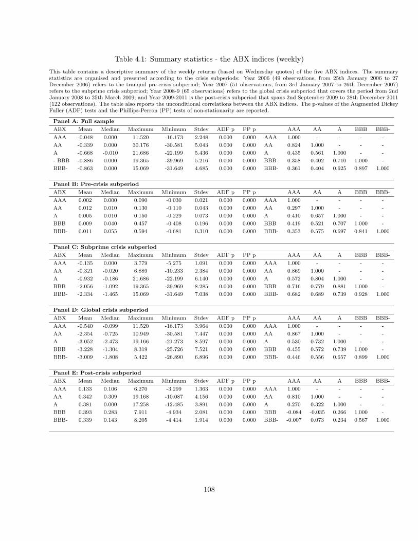
Table 4.1: Summary statistics - the ABX indices (weekly)
This table contains a descriptive summary of the weekly returns (based on Wednesday quotes) of the five ABX indices. The summarystatistics are organised and presented according to the crisis subperiods: Year 2006 (49 observations, from 25th January 2006 to 27December 2006) refers to the tranquil pre-crisis subperiod; Year 2007 (51 observations, from 3rd January 2007 to 26th December 2007)refers to the subprime crisis subperiod; Year 2008-9 (65 observations) refers to the global crisis subperiod that covers the period from 2ndJanuary 2008 to 25th March 2009; and Year 2009-2011 is the post-crisis subperiod that spans 2nd September 2009 to 28th December 2011(122 observations). The table also reports the unconditional correlations between the ABX indices. The p-values of the Augmented DickeyFuller (ADF) tests and the Phillips-Perron (PP) tests of non-stationarity are reported.
Panel A: Full sample
ABX Mean Median Maximum Minimum Stdev ADF p PP p AAA AA A BBB BBB-
AAA -0.048 0.000 11.520 -16.173 2.248 0.000 0.000 AAA 1.000 - - - -
AA -0.339 0.000 30.176 -30.581 5.043 0.000 0.000 AA 0.824 1.000 - - -
A -0.668 -0.010 21.686 -22.199 5.436 0.000 0.000 A 0.435 0.561 1.000 - -
- BBB -0.886 0.000 19.365 -39.969 5.216 0.000 0.000 BBB 0.358 0.402 0.710 1.000 -
BBB- -0.863 0.000 15.069 -31.649 4.685 0.000 0.000 BBB- 0.361 0.404 0.625 0.897 1.000
Panel B: Pre-crisis subperiod
ABX Mean Median Maximum Minimum Stdev ADF p PP p AAA AA A BBB BBB-
AAA 0.002 0.000 0.090 -0.030 0.021 0.000 0.000 AAA 1.000 - - - -
AA 0.012 0.010 0.130 -0.110 0.043 0.000 0.000 AA 0.297 1.000 - - -
A 0.005 0.010 0.150 -0.229 0.073 0.000 0.000 A 0.410 0.657 1.000 - -
BBB 0.009 0.040 0.457 -0.408 0.196 0.000 0.000 BBB 0.419 0.521 0.707 1.000 -
BBB- 0.011 0.055 0.594 -0.681 0.310 0.000 0.000 BBB- 0.353 0.575 0.697 0.841 1.000
Panel C: Subprime crisis subperiod
ABX Mean Median Maximum Minimum Stdev ADF p PP p AAA AA A BBB BBB-
AAA -0.135 0.000 3.779 -5.275 1.091 0.000 0.000 AAA 1.000 - - - -
AA -0.321 -0.020 6.889 -10.233 2.384 0.000 0.000 AA 0.869 1.000 - - -
A -0.932 -0.186 21.686 -22.199 6.140 0.000 0.000 A 0.572 0.804 1.000 - -
BBB -2.056 -1.092 19.365 -39.969 8.285 0.000 0.000 BBB 0.716 0.779 0.881 1.000 -
BBB- -2.334 -1.465 15.069 -31.649 7.038 0.000 0.000 BBB- 0.682 0.689 0.739 0.928 1.000
Panel D: Global crisis subperiod
ABX Mean Median Maximum Minimum Stdev ADF p PP p AAA AA A BBB BBB-
AAA -0.540 -0.099 11.520 -16.173 3.964 0.000 0.000 AAA 1.000 - - - -
AA -2.354 -0.725 10.949 -30.581 7.447 0.000 0.000 AA 0.867 1.000 - - -
A -3.052 -2.473 19.166 -21.273 8.597 0.000 0.000 A 0.530 0.732 1.000 - -
BBB -3.228 -1.304 8.319 -25.726 7.521 0.000 0.000 BBB 0.455 0.572 0.739 1.000 -
BBB- -3.009 -1.808 5.422 -26.890 6.896 0.000 0.000 BBB- 0.446 0.556 0.657 0.899 1.000
Panel E: Post-crisis subperiod
ABX Mean Median Maximum Minimum Stdev ADF p PP p AAA AA A BBB BBB-
AAA 0.133 0.106 6.270 -3.299 1.363 0.000 0.000 AAA 1.000 - - - -
AA 0.342 0.309 19.168 -10.087 4.156 0.000 0.000 AA 0.810 1.000 - - -
A 0.381 0.000 17.258 -12.485 3.891 0.000 0.000 A 0.270 0.322 1.000 - -
BBB 0.393 0.283 7.911 -4.934 2.081 0.000 0.000 BBB -0.084 -0.035 0.266 1.000 -
BBB- 0.339 0.143 8.205 -4.414 1.914 0.000 0.000 BBB- -0.007 0.073 0.234 0.567 1.000
108
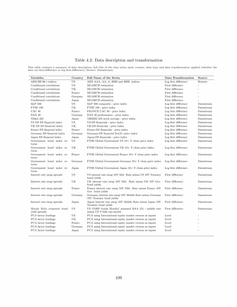
Table 4.2: Data description and transformation
This table contains a summary of data description, full title of the time series used, country, data type and data transformation applied (whether thedata are first-difference or log first-difference) (Source: Datastream).
Variables Country Full Name of the Series Data Transformation Source
ABX.HE.06-1 indices US ABX AAA, AA, A, BBB and BBB- indices Log first difference Reuters
Conditional correlations US MGARCH estimation First difference -
Conditional correlations UK MGARCH estimation First difference -
Conditional correlations France MGARCH estimation First difference -
Conditional correlations Germany MGARCH estimation First difference -
Conditional correlations Japan MGARCH estimation First difference -
S&P 500 US S&P 500 composite - price index Log first difference Datastream
FTSE 100 UK FTSE 100 - price index Log first difference Datastream
CAC 40 France FRANCE CAC 40 - price index Log first difference Datastream
DAX 30 Germany DAX 30 performance - price index Log first difference Datastream
Nikkei 225 Japan NIKKEI 225 stock average - price index Log first difference Datastream
US DS DS financial index US US-DS financials - price index Log first difference Datastream
UK DS DS financial index UK UK-DS financials - price index Log first difference Datastream
France DS financial index France France-DS financials - price index Log first difference Datastream
Germany DS financial index Germany Germany-DS financial Svs(3) -price index Log first difference Datastream
Japan DS financial index Japan Japan-DS financials - price index Log first difference Datastream
Government bond index re-turns
US FTSE Global Government US 10+ Y clean price index Log first difference Datastream
Government bond index re-turns
UK FTSE Global Government UK 10+ Y clean price index Log first difference Datastream
Government bond index re-turns
France FTSE Global Government France 10+ Y clean price index Log first difference Datastream
Government bond index re-turns
Germany FTSE Global Government Germany 10+ Y clean price index Log first difference Datastream
Government bond index re-turns
Japan FTSE Global Government Japan 10+ Y clean price index Log first difference Datastream
Interest rate swap spreads US US interest rate swap 10Y Mid. Rate minus US 10Y Treasurybond yields
First difference Datastream
Interest rate swap spreads UK UK interest rate swap 10Y Mid. Rate minus UK 10Y Gov.bond yields
First difference Datastream
Interest rate swap spreads France France interest rate swap 10Y Mid. Rate minus France 10YGov. bond yields
First difference Datastream
Interest rate swap spreads Germany Germany interest rate swap 10Y Middle Rate minus Germany10Y Treasury bond yields
First difference Datastream
Interest rate swap spreads Japan Japan interest rate swap 10Y Middle Rate minus Japan 10YTreasury bond yields
First difference Datastream
Moody BAA corporate bondyield spreads
US US CORP bonds Moodys’ seasoned BAA (D) - middle rateminus US T-bills one-month
First difference Datastream
PCA factor loadings US PCA using International equity market returns as inputs Level -
PCA factor loadings UK PCA using International equity market returns as inputs Level -
PCA factor loadings France PCA using International equity market returns as inputs Level -
PCA factor loadings Germany PCA using International equity market returns as inputs Level -
PCA factor loadings Japan PCA using International equity market returns as inputs Level -
109
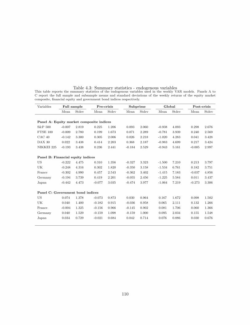
Table 4.3: Summary statistics - endogenous variablesThis table reports the summary statistics of the endogenous variables used in the weekly VAR models. Panels A toC report the full sample and subsample means and standard deviations of the weekly returns of the equity marketcomposite, financial equity and government bond indices respectively.
Variables Full sample Pre-crisis Subprime Global Post-crisis
Mean Stdev Mean Stdev Mean Stdev Mean Stdev Mean Stdev
Panel A: Equity market composite indices
S&P 500 -0.007 2.819 0.225 1.206 0.093 2.060 -0.938 4.093 0.298 2.676
FTSE 100 -0.009 2.780 0.199 1.673 0.071 2.289 -0.781 3.939 0.240 2.569
CAC 40 -0.142 3.300 0.305 2.006 0.026 2.218 -1.020 4.283 0.041 3.428
DAX 30 0.022 3.438 0.414 2.203 0.368 2.187 -0.983 4.699 0.217 3.424
NIKKEI 225 -0.193 3.438 0.236 2.441 -0.184 2.529 -0.943 5.161 -0.005 2.997
Panel B: Financial equity indices
US -0.222 4.475 0.310 1.356 -0.327 3.323 -1.500 7.210 0.213 3.797
UK -0.248 4.316 0.302 1.820 -0.350 3.158 -1.534 6.761 0.182 3.751
France -0.302 4.990 0.457 2.543 -0.362 3.402 -1.415 7.183 -0.037 4.856
Germany -0.194 3.739 0.419 2.201 -0.055 2.456 -1.225 5.584 0.011 3.437
Japan -0.442 4.473 -0.077 3.035 -0.474 3.977 -1.064 7.219 -0.273 3.306
Panel C: Government bond indices
US 0.074 1.378 -0.073 0.873 0.030 0.964 0.167 1.672 0.098 1.502
UK 0.040 1.400 -0.182 0.915 -0.036 0.958 0.065 2.111 0.132 1.266
France -0.004 1.325 -0.156 0.966 -0.145 0.902 0.081 1.706 0.060 1.366
Germany 0.040 1.529 -0.159 1.098 -0.159 1.000 0.095 2.034 0.155 1.548
Japan 0.034 0.729 -0.021 0.684 0.042 0.714 0.076 0.886 0.030 0.676
110
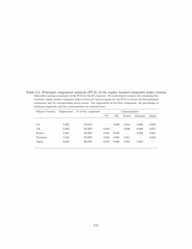
Table 4.4: Principal component analysis (PCA) of the equity market composite index returnsThis table contains a summary of the PCA for the G5 countries. For each subject country, the remaining four
countries’ equity market composite index returns are used as inputs for the PCA to obtain the first principal
component and its corresponding factor scores. The eigenvalues of the first component, the percentage of
variances explained, and the commonalities are reported here.
Subject Country Eigenvalues % of Var. explained Communalities
US UK France Germany Japan
US 3.392 84.81% - 0.889 0.944 0.909 0.650
UK 3.303 82.56% 0.819 - 0.930 0.898 0.655
France 3.255 83.38% 0.841 0.895 - 0.868 0.651
Germany 3.312 82.80% 0.848 0.905 0.911 - 0.648
Japan 3.625 90.64% 0.847 0.920 0.951 0.907 -
111
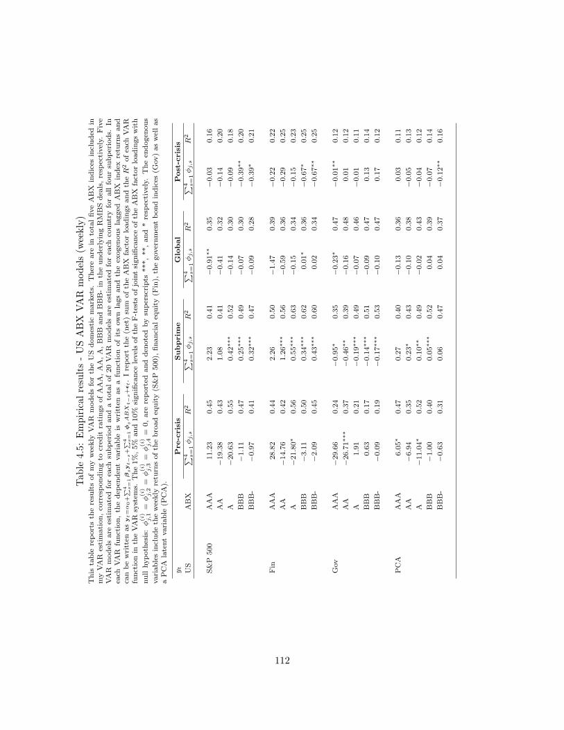
Tab
le4.5:Empiricalresults-USABX
VAR
models(w
eekly)
This
table
reportsth
eresu
ltsofmyweekly
VAR
modelsforth
eUSdomesticmarkets.
Thereare
intotalfiveABX
indices
included
inmyVAR
estimation,co
rrespondingto
cred
itratingsofAAA,AA,A,BBB
andBBB-in
theunderlyingRMBSdea
ls,resp
ectively.
Five
VAR
modelsare
estimatedforea
chsu
bperiodandatotalof20VAR
modelsare
estimatedforea
chco
untryforallfoursu
bperiods.
Inea
chVAR
function,th
edep
enden
tvariable
iswritten
asafunction
ofitsown
lagsand
theex
ogen
ouslagged
ABX
index
retu
rnsand
canbewritten
as
yt=α0+∑ 4 s
=1βsyt−
s+∑ 4 s
=1ϕ
sABX
t−
s+ϵt.Ireport
the(n
et)su
mofth
eABX
factorloadingsandth
eR
2ofea
chVAR
functionin
theVAR
system
s.The1%,5%
and10%
significa
nce
levelsofth
eF-tests
ofjointsignifica
nce
ofth
eABX
factorloadingswith
nullhypoth
esis:ϕ(i)
j,1
=ϕ(i)
j,2
=ϕ(i)
j,3
=ϕ(i)
j,4
=0,are
reported
andden
otedbysu
perscripts
***,**,and*resp
ectively.
Theen
dogen
ous
variablesincludeth
eweekly
retu
rnsofth
ebroadeq
uity(S
&P
500),
financialeq
uity(F
in),
thegovernmen
tbondindices
(Gov)aswellas
aPCA
latentvariable
(PCA).
yt
Pre-crisis
Subprim
eGlobal
Post-crisis
US
ABX
∑ 4 s=1ϕj,s
R2
∑ 4 s=1ϕj,s
R2
∑ 4 s=1ϕj,s
R2
∑ 4 s=1ϕj,s
R2
S&P
500
AAA
11.23
0.45
2.23
0.41
−0.91∗∗
0.35
−0.03
0.16
AA
−19.38
0.43
1.08
0.41
−0.41
0.32
−0.14
0.20
A−20.63
0.55
0.42∗∗
∗0.52
−0.14
0.30
−0.09
0.18
BBB
−1.11
0.47
0.25∗∗
∗0.49
−0.07
0.30
−0.39∗∗
0.20
BBB-
−0.97
0.41
0.32∗∗
∗0.47
−0.09
0.28
−0.39∗
0.21
Fin
AAA
28.82
0.44
2.26
0.50
−1.47
0.39
−0.22
0.22
AA
−14.76
0.42
1.26∗∗
∗0.56
−0.59
0.36
−0.29
0.25
A−21.80∗
0.56
0.55∗∗
∗0.63
−0.15
0.34
−0.15
0.23
BBB
−3.11
0.50
0.34∗∗
∗0.62
0.01∗
0.36
−0.67∗
0.25
BBB-
−2.09
0.45
0.43∗∗
∗0.60
0.02
0.34
−0.67∗∗
0.25
Gov
AAA
−29.66
0.24
−0.95∗
0.35
−0.23∗
0.47
−0.01∗∗
0.12
AA
−26.71∗∗
∗0.37
−0.46∗∗
0.39
−0.16
0.48
0.01
0.12
A1.91
0.21
−0.19∗∗
∗0.49
−0.07
0.46
−0.01
0.11
BBB
0.63
0.17
−0.14∗∗
∗0.51
−0.09
0.47
0.13
0.14
BBB-
−0.09
0.19
−0.17∗∗
∗0.53
−0.10
0.47
0.17
0.12
PCA
AAA
6.05∗
0.47
0.27
0.40
−0.13
0.36
0.03
0.11
AA
−6.94
0.35
0.23∗
0.43
−0.10
0.38
−0.05
0.13
A−11.04∗
0.52
0.10∗∗
0.49
−0.02
0.43
−0.04
0.12
BBB
−1.00
0.40
0.05∗∗
∗0.52
0.04
0.39
−0.07
0.14
BBB-
−0.63
0.31
0.06
0.47
0.04
0.37
−0.12∗∗
0.16
112
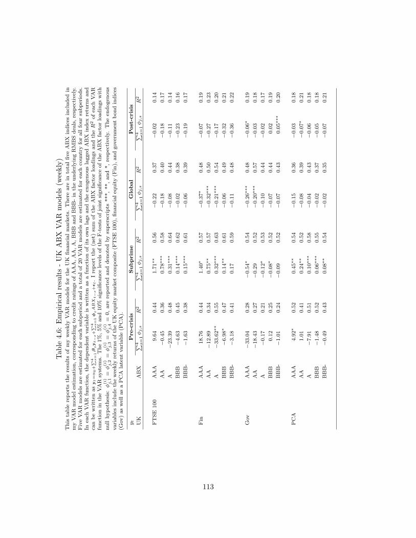
Tab
le4.6:Empiricalresults-UK
ABX
VAR
models(w
eekly)
This
table
reportsth
eresu
ltsofmyweekly
VAR
modelsforth
eUK
financialmarkets.
Thereare
intotalfiveABX
indices
included
inmyVAR
model
estimation,co
rrespondingto
cred
itratingsofAAA,AA,A,BBB
andBBB-in
theunderlyingRMBSdea
ls,resp
ectively.
FiveVAR
modelsare
estimatedforea
chsu
bperiodandatotalof20VAR
modelsare
estimatedforea
chco
untryforallfoursu
bperiods.
Inea
chVAR
function,th
edep
enden
tvariable
iswritten
asafunctionofitsownlagsandth
eex
ogen
ouslagged
ABX
index
retu
rnsand
canbewritten
as
yt=α0+∑ 4 s
=1βsyt−
s+∑ 4 s
=1ϕ
sABX
t−
s+ϵt.Ireport
the(n
et)su
mofth
eABX
factorloadingsandth
eR
2ofea
chVAR
functionin
theVAR
system
s.The1%,5%
and10%
significa
nce
levelsofth
eF-tests
ofjointsignifica
nce
ofth
eABX
factorloadingswith
nullhypoth
esis:ϕ(i)
j,1
=ϕ(i)
j,2
=ϕ(i)
j,3
=ϕ(i)
j,4
=0,are
reported
andden
otedbysu
perscripts
***,**,and*,resp
ectively.
Theen
dogen
ous
variablesincludeth
eweekly
retu
rnsofth
eUK
equitymarket
composite
(FTSE
100),
financialeq
uity(F
in),
andgovernmen
tbondindices
(Gov)aswellasaPCA
latentvariable
(PCA).
yt
Pre-crisis
Subprim
eGlobal
Post-crisis
UK
ABX
∑ 4 s=1ϕj,s
R2
∑ 4 s=1ϕj,s
R2
∑ 4 s=1ϕj,s
R2
∑ 4 s=1ϕj,s
R2
FTSE
100
AAA
9.64
0.44
1.71∗∗
0.56
−0.22
0.37
−0.02
0.14
AA
−0.45
0.36
0.78∗∗
∗0.58
−0.18
0.40
−0.18
0.17
A−23.39
0.48
0.31∗∗
∗0.64
−0.08
0.44
−0.11
0.14
BBB
−4.63
0.45
0.14∗∗
∗0.62
−0.02
0.38
−0.23
0.16
BBB-
−1.63
0.38
0.15∗∗
∗0.61
−0.06
0.39
−0.19
0.17
Fin
AAA
18.76
0.44
1.40∗
0.57
−0.37∗
0.48
−0.07
0.19
AA
−12.89
0.34
0.75∗∗
0.57
−0.32∗∗
∗0.50
−0.27
0.23
A−33.62∗∗
0.55
0.32∗∗
∗0.63
−0.21∗∗
∗0.54
−0.17
0.20
BBB
−6.98∗
0.47
0.14∗∗
0.61
−0.06
0.49
−0.32
0.21
BBB-
−3.18
0.41
0.17
0.59
−0.11
0.48
−0.36
0.22
Gov
AAA
−33.04
0.28
−0.54∗
0.54
−0.26∗∗
∗0.48
−0.06∗
0.19
AA
−18.43
0.27
−0.29
0.52
−0.20∗∗
∗0.57
−0.03
0.18
A−0.17
0.21
−0.12∗
0.53
−0.10
0.44
−0.02
0.17
BBB
0.12
0.25
−0.08∗
0.52
−0.07
0.44
0.02
0.19
BBB-
−1.01
0.24
−0.09
0.52
−0.07
0.43
0.05∗∗
∗0.20
PCA
AAA
4.92∗
0.52
0.45∗∗
0.54
−0.15
0.36
−0.03
0.18
AA
1.01
0.41
0.24∗∗
0.52
−0.08
0.39
−0.07∗
0.21
A−7.91
0.51
0.10∗∗
∗0.58
−0.04
0.43
−0.06
0.18
BBB
−1.48
0.52
0.06∗∗
∗0.55
−0.02
0.37
−0.05
0.18
BBB-
−0.49
0.43
0.08∗∗
0.54
−0.02
0.35
−0.07
0.21
113

Tab
le4.7:Empiricalresults-France
ABX
VAR
models(w
eekly)
This
table
reportsth
eresu
ltsofmyweekly
VAR
modelsforth
eFrench
financialmarkets.
Thereare
intotalfiveABX
indices
included
inmyVAR
model
estimation,co
rrespondingto
cred
itratingsofAAA,AA,A,BBB
andBBB-in
theunderlyingRMBSdea
lsresp
ectively.
FiveVAR
modelsare
estimatedforea
chsu
bperiodandatotalof20VAR
modelsare
estimatedforea
chco
untryforallfoursu
bperiods.
Inea
chVAR
function,th
edep
enden
tvariable
iswritten
asafunctionofitsownlagsandth
eex
ogen
ouslagged
ABX
index
retu
rnsand
canbewritten
as
yt=α0+∑ 4 s
=1βsyt−
s+∑ 4 s
=1ϕ
sABX
t−
s+ϵt.Ireport
the(n
et)su
mofth
eABX
factorloadingsandth
eR
2ofea
chVAR
functionin
theVAR
system
s.The1%,5%
and10%
significa
nce
levelsofth
eF-tests
ofjointsignifica
nce
ofth
eABX
factorloadingswith
nullhypoth
esis:ϕ(i)
j,1
=ϕ(i)
j,2
=ϕ(i)
j,3
=ϕ(i)
j,4
=0,are
reported
and
den
oted
bysu
perscripts
***,**,and
*resp
ectively.
Theen
dogen
ous
variablesincludeth
eweekly
retu
rnsofth
eFrench
equitymarket
composite
(CAC
40),
financialeq
uity(F
in),
andgovernmen
tbondindices
(Gov)aswellasaPCA
latentvariable
(PCA).
yt
Pre-crisis
Subprim
eGlobal
Post-crisis
France
ABX
∑ 4 s=1ϕj,s
R2
∑ 4 s=1ϕj,s
R2
∑ 4 s=1ϕj,s
R2
∑ 4 s=1ϕj,s
R2
CAC
40
AAA
40.47∗
0.51
3.06∗∗
∗0.48
−1.05
0.43
0.26∗∗
0.22
AA
17.61
0.41
1.08∗∗
∗0.46
−0.35
0.41
−0.10
0.22
A−24.54
0.52
0.49∗∗
∗0.53
−0.10
0.42
−0.11
0.20
BBB
0.42
0.40
0.25∗∗
∗0.50
0.03
0.36
−0.04
0.20
BBB-
1.36
0.36
0.21∗∗
0.43
0.14
0.36
−0.24
0.21
Fin
AAA
53.40∗
0.38
2.95∗∗
0.52
−1.68∗∗
0.51
0.32∗∗
0.22
AA
25.97
0.30
1.31∗∗
∗0.53
−0.42
0.45
−0.10∗
0.22
A−34.01∗
0.44
0.63∗∗
∗0.61
−0.16
0.44
−0.12
0.20
BBB
−0.22
0.28
0.31∗∗
∗0.60
0.06
0.40
0.01
0.20
BBB-
1.58
0.27
0.26∗
0.53
0.24
0.40
−0.22
0.20
Gov
AAA
−66.99
0.33
−0.94∗
0.41
−0.25∗∗
0.35
−0.07
0.07
AA
−27.32∗∗
∗0.33
−0.29∗∗
0.40
−0.16∗∗
∗0.42
0.00
0.09
A−2.47
0.18
−0.14∗∗
∗0.49
−0.07
0.28
0.05
0.09
BBB
−0.16
0.18
−0.13∗∗
∗0.53
−0.09
0.34
0.13
0.09
BBB-
−0.37
0.18
−0.15∗∗
∗0.53
−0.12
0.37
0.15
0.08
PCA
AAA
12.12∗
0.47
1.03∗∗
∗0.47
−0.37
0.43
0.07
0.18
AA
4.57
0.36
0.39∗∗
∗0.49
−0.14∗
0.42
−0.03
0.18
A−6.77
0.48
0.18∗∗
∗0.60
−0.05
0.39
−0.03
0.17
BBB
0.04
0.41
0.09∗∗
∗0.55
−0.01
0.34
−0.05
0.17
BBB-
0.46
0.37
0.08∗∗
∗0.47
0.00
0.34
−0.10
0.18
114
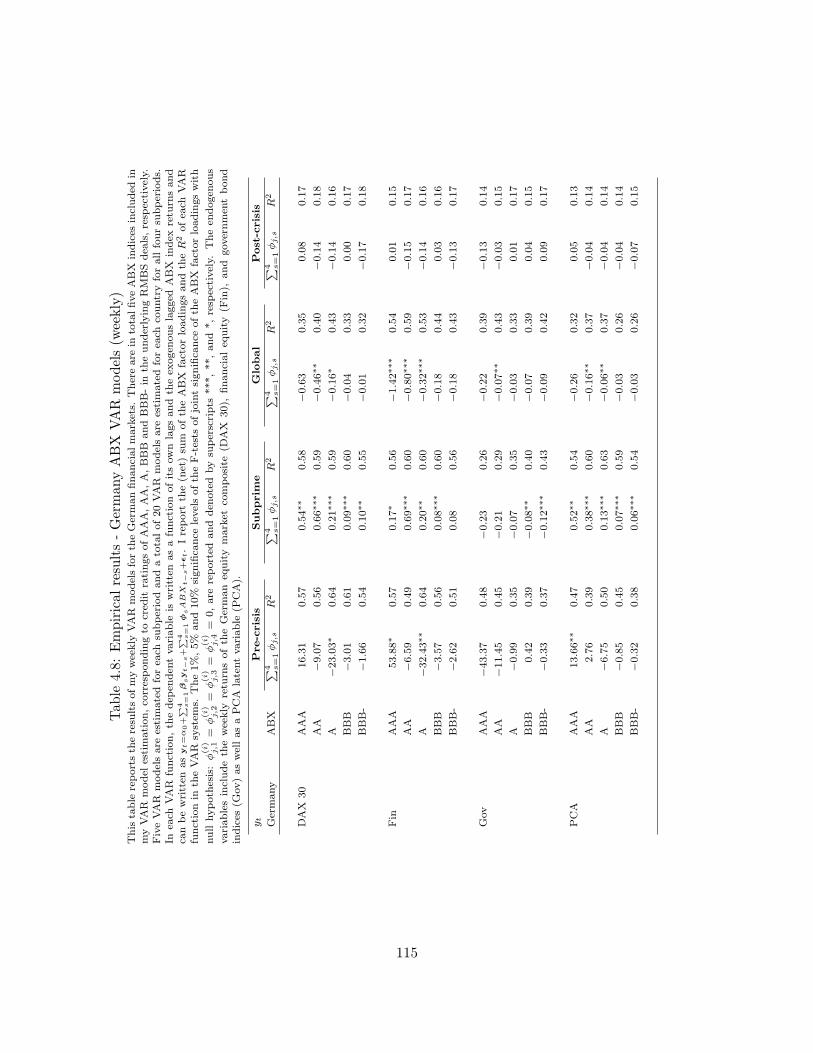
Tab
le4.8:Empiricalresults-GermanyABX
VAR
models(w
eekly)
This
table
reportsth
eresu
ltsofmyweekly
VAR
modelsforth
eGermanfinancialmarkets.
Thereare
intotalfiveABX
indices
included
inmyVAR
model
estimation,co
rrespondingto
cred
itratingsofAAA,AA,A,BBB
andBBB-in
theunderlyingRMBSdea
ls,resp
ectively.
FiveVAR
modelsare
estimatedforea
chsu
bperiodandatotalof20VAR
modelsare
estimatedforea
chco
untryforallfoursu
bperiods.
Inea
chVAR
function,th
edep
enden
tvariable
iswritten
asafunctionofitsownlagsandth
eex
ogen
ouslagged
ABX
index
retu
rnsand
canbewritten
as
yt=α0+∑ 4 s
=1βsyt−
s+∑ 4 s
=1ϕ
sABX
t−
s+ϵt.Ireport
the(n
et)su
mofth
eABX
factorloadingsandth
eR
2ofea
chVAR
functionin
theVAR
system
s.The1%,5%
and10%
significa
nce
levelsofth
eF-tests
ofjointsignifica
nce
ofth
eABX
factorloadingswith
nullhypoth
esis:ϕ(i)
j,1
=ϕ(i)
j,2
=ϕ(i)
j,3
=ϕ(i)
j,4
=0,are
reported
andden
otedbysu
perscripts
***,**,and*,resp
ectively.
Theen
dogen
ous
variablesincludeth
eweekly
retu
rnsofth
eGerman
equity
market
composite
(DAX
30),
financialeq
uity
(Fin),
and
governmen
tbond
indices
(Gov)aswellasaPCA
latentvariable
(PCA).
yt
Pre-crisis
Subprim
eGlobal
Post-crisis
Germany
ABX
∑ 4 s=1ϕj,s
R2
∑ 4 s=1ϕj,s
R2
∑ 4 s=1ϕj,s
R2
∑ 4 s=1ϕj,s
R2
DAX
30
AAA
16.31
0.57
0.54∗∗
0.58
−0.63
0.35
0.08
0.17
AA
−9.07
0.56
0.66∗∗
∗0.59
−0.46∗∗
0.40
−0.14
0.18
A−23.03∗
0.64
0.21∗∗
∗0.59
−0.16∗
0.43
−0.14
0.16
BBB
−3.01
0.61
0.09∗∗
∗0.60
−0.04
0.33
0.00
0.17
BBB-
−1.66
0.54
0.10∗∗
0.55
−0.01
0.32
−0.17
0.18
Fin
AAA
53.88∗
0.57
0.17∗
0.56
−1.42∗∗
∗0.54
0.01
0.15
AA
−6.59
0.49
0.69∗∗
∗0.60
−0.80∗∗
∗0.59
−0.15
0.17
A−32.43∗∗
0.64
0.20∗∗
0.60
−0.32∗∗
∗0.53
−0.14
0.16
BBB
−3.57
0.56
0.08∗∗
∗0.60
−0.18
0.44
0.03
0.16
BBB-
−2.62
0.51
0.08
0.56
−0.18
0.43
−0.13
0.17
Gov
AAA
−43.37
0.48
−0.23
0.26
−0.22
0.39
−0.13
0.14
AA
−11.45
0.45
−0.21
0.29
−0.07∗∗
0.43
−0.03
0.15
A−0.99
0.35
−0.07
0.35
−0.03
0.33
0.01
0.17
BBB
0.42
0.39
−0.08∗∗
0.40
−0.07
0.39
0.04
0.15
BBB-
−0.33
0.37
−0.12∗∗
∗0.43
−0.09
0.42
0.09
0.17
PCA
AAA
13.66∗∗
0.47
0.52∗∗
0.54
−0.26
0.32
0.05
0.13
AA
2.76
0.39
0.38∗∗
∗0.60
−0.16∗∗
0.37
−0.04
0.14
A−6.75
0.50
0.13∗∗
∗0.63
−0.06∗∗
0.37
−0.04
0.14
BBB
−0.85
0.45
0.07∗∗
∗0.59
−0.03
0.26
−0.04
0.14
BBB-
−0.32
0.38
0.06∗∗
∗0.54
−0.03
0.26
−0.07
0.15
115
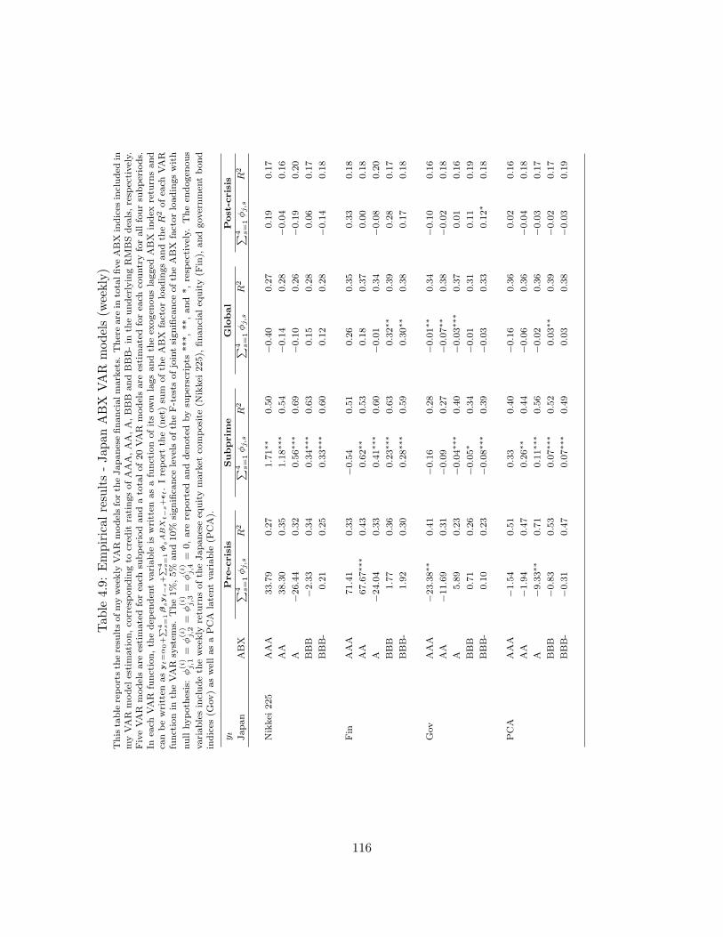
Tab
le4.9:Empiricalresults-JapanABX
VAR
models(w
eekly)
Thistable
reportsth
eresu
ltsofmyweekly
VAR
modelsforth
eJapanesefinancialmarkets.
Thereare
intotalfiveABX
indices
included
inmyVAR
model
estimation,co
rrespondingto
cred
itratingsofAAA,AA,A,BBB
andBBB-in
theunderlyingRMBSdea
ls,resp
ectively.
FiveVAR
modelsare
estimatedforea
chsu
bperiodandatotalof20VAR
modelsare
estimatedforea
chco
untryforallfoursu
bperiods.
Inea
chVAR
function,th
edep
enden
tvariable
iswritten
asafunctionofitsownlagsandth
eex
ogen
ouslagged
ABX
index
retu
rnsand
canbewritten
as
yt=α0+∑ 4 s
=1βsyt−
s+∑ 4 s
=1ϕ
sABX
t−
s+ϵt.Ireport
the(n
et)su
mofth
eABX
factorloadingsandth
eR
2ofea
chVAR
functionin
theVAR
system
s.The1%,5%
and10%
significa
nce
levelsofth
eF-tests
ofjointsignifica
nce
ofth
eABX
factorloadingswith
nullhypoth
esis:ϕ(i)
j,1
=ϕ(i)
j,2
=ϕ(i)
j,3
=ϕ(i)
j,4
=0,are
reported
andden
otedbysu
perscripts
***,**,and*,resp
ectively.
Theen
dogen
ous
variablesincludeth
eweekly
retu
rnsofth
eJapaneseeq
uitymarket
composite
(Nikkei
225),
financialeq
uity(F
in),
andgovernmen
tbond
indices
(Gov)aswellasaPCA
latentvariable
(PCA).
yt
Pre-crisis
Subprim
eGlobal
Post-crisis
Japan
ABX
∑ 4 s=1ϕj,s
R2
∑ 4 s=1ϕj,s
R2
∑ 4 s=1ϕj,s
R2
∑ 4 s=1ϕj,s
R2
Nikkei
225
AAA
33.79
0.27
1.71∗∗
0.50
−0.40
0.27
0.19
0.17
AA
38.30
0.35
1.18∗∗
∗0.54
−0.14
0.28
−0.04
0.16
A−26.44
0.32
0.56∗∗
∗0.69
−0.10
0.26
−0.19
0.20
BBB
−2.33
0.34
0.34∗∗
∗0.63
0.15
0.28
0.06
0.17
BBB-
0.21
0.25
0.33∗∗
∗0.60
0.12
0.28
−0.14
0.18
Fin
AAA
71.41
0.33
−0.54
0.51
0.26
0.35
0.33
0.18
AA
67.67∗∗
∗0.43
0.62∗∗
0.53
0.18
0.37
0.00
0.18
A−24.04
0.33
0.41∗∗
∗0.60
−0.01
0.34
−0.08
0.20
BBB
1.77
0.36
0.23∗∗
∗0.63
0.32∗∗
0.39
0.28
0.17
BBB-
1.92
0.30
0.28∗∗
∗0.59
0.30∗∗
0.38
0.17
0.18
Gov
AAA
−23.38∗∗
0.41
−0.16
0.28
−0.01∗∗
0.34
−0.10
0.16
AA
−11.69
0.31
−0.09
0.27
−0.07∗∗
0.38
−0.02
0.18
A5.89
0.23
−0.04∗∗
∗0.40
−0.03∗∗
∗0.37
0.01
0.16
BBB
0.71
0.26
−0.05∗
0.34
−0.01
0.31
0.11
0.19
BBB-
0.10
0.23
−0.08∗∗
∗0.39
−0.03
0.33
0.12∗
0.18
PCA
AAA
−1.54
0.51
0.33
0.40
−0.16
0.36
0.02
0.16
AA
−1.94
0.47
0.26∗∗
0.44
−0.06
0.36
−0.04
0.18
A−9.33∗∗
0.71
0.11∗∗
∗0.56
−0.02
0.36
−0.03
0.17
BBB
−0.83
0.53
0.07∗∗
∗0.52
0.03∗∗
0.39
−0.02
0.17
BBB-
−0.31
0.47
0.07∗∗
∗0.49
0.03
0.38
−0.03
0.19
116
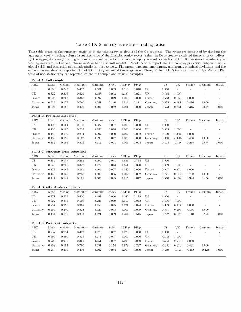
Table 4.10: Summary statistics - trading ratios
This table contains the summary statistics of the trading ratios (level) of the G5 countries. The ratios are computed by dividing theaggregate weekly trading volume in market value of the financial equity sector (using the Datastream-calculated financial price indices)by the aggregate weekly trading volume in market value for the broader equity market for each country. It measures the intensity oftrading activities in financial stocks relative to the overall market. Panels A to E report the full sample, pre-crisis, subprime crisis,global crisis and post-crisis subsample statistics, respectively. The means, medians, maximums, minimums, standard deviations and thecorrelation matrices are reported. In addition, the p-values of the Augmented Dickey Fuller (ADF) tests and the Phillips-Perron (PP)tests of non-stationarity are reported for the full sample and crisis subsamples.
Panel A: Full sample
ABX Mean Median Maximum Minimum Stdev ADF p PP p US UK France Germany Japan
US 0.233 0.242 0.482 0.087 0.089 0.110 0.010 US 1.000 - - - -
UK 0.322 0.336 0.529 0.153 0.093 0.189 0.021 UK 0.765 1.000 - - -
France 0.206 0.207 0.368 0.097 0.049 0.000 0.000 France 0.563 0.630 1.000 - -
Germany 0.225 0.177 0.760 0.051 0.140 0.916 0.111 Germany 0.252 0.481 0.476 1.000 -
Japan 0.204 0.192 0.436 0.104 0.062 0.001 0.000 Japan 0.673 0.631 0.315 0.072 1.000
Panel B: Pre-crisis subperiod
ABX Mean Median Maximum Minimum Stdev ADF p PP p US UK France Germany Japan
US 0.103 0.104 0.116 0.087 0.007 0.000 0.000 US 1.000 - - - -
UK 0.186 0.183 0.223 0.153 0.018 0.000 0.000 UK 0.089 1.000 - - -
France 0.150 0.149 0.214 0.097 0.030 0.002 0.002 France 0.190 -0.045 1.000 - -
Germany 0.130 0.128 0.162 0.090 0.017 0.000 0.000 Germany 0.068 -0.013 0.406 1.000 -
Japan 0.156 0.156 0.212 0.115 0.021 0.005 0.004 Japan 0.103 -0.156 0.255 0.075 1.000
Panel C: Subprime crisis subperiod
ABX Mean Median Maximum Minimum Stdev ADF p PP p US UK France Germany Japan
US 0.157 0.147 0.252 0.099 0.041 0.685 0.754 US 1.000 - - - -
UK 0.245 0.235 0.342 0.172 0.044 0.651 0.320 UK 0.809 1.000 - - -
France 0.172 0.169 0.261 0.104 0.037 0.043 0.060 France 0.817 0.774 1.000 - -
Germany 0.149 0.138 0.258 0.100 0.035 0.002 0.002 Germany 0.721 0.672 0.708 1.000 -
Japan 0.147 0.142 0.191 0.104 0.025 0.015 0.017 Japan 0.560 0.602 0.394 0.456 1.000
Panel D: Global crisis subperiod
ABX Mean Median Maximum Minimum Stdev ADF p PP p US UK France Germany Japan
US 0.271 0.259 0.430 0.187 0.060 0.143 0.179 US 1.000 - - - -
UK 0.322 0.315 0.509 0.224 0.059 0.019 0.033 UK 0.636 1.000 - - -
France 0.237 0.236 0.368 0.156 0.045 0.021 0.024 France 0.389 0.417 1.000 - -
Germany 0.264 0.240 0.524 0.120 0.093 0.006 0.009 Germany 0.341 0.295 -0.059 1.000 -
Japan 0.184 0.177 0.313 0.121 0.039 0.484 0.545 Japan 0.722 0.625 0.140 0.225 1.000
Panel E: Post-crisis subperiod
ABX Mean Median Maximum Minimum Stdev ADF p PP p US UK France Germany Japan
US 0.287 0.274 0.482 0.178 0.057 0.020 0.000 US 1.000 - - - -
UK 0.396 0.390 0.529 0.277 0.047 0.000 0.000 UK -0.048 1.000 - - -
France 0.223 0.217 0.361 0.151 0.037 0.000 0.000 France -0.251 0.248 1.000 - -
Germany 0.268 0.194 0.760 0.051 0.174 0.978 0.237 Germany -0.383 0.320 0.431 1.000 -
Japan 0.250 0.239 0.436 0.162 0.054 0.000 0.000 Japan 0.369 -0.128 -0.188 -0.423 1.000
117
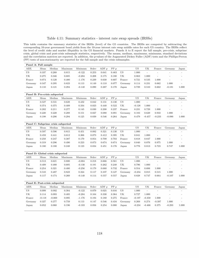
Table 4.11: Summary statistics - interest rate swap spreads (IRSSs)
This table contains the summary statistics of the IRSSs (level) of the G5 countries. The IRSSs are computed by subtracting thecorresponding 10-year government bond yields from the 10-year interest rate swap middle rates for each G5 country. The IRSSs reflectthe level of credit risks and market illiquidity in the G5 financial markets. Panels A to E report the full sample, pre-crisis, subprimecrisis, global crisis and post-crisis subsample statistics, respectively. The means, medians, maximums, minimums, standard deviationsand the correlation matrices are reported. In addition, the p-values of the Augmented Dickey Fuller (ADF) tests and the Phillips-Perron(PP) tests of non-stationarity are reported for the full sample and the crisis subsamples.
Panel A: Full sample
ABX Mean Median Maximum Minimum Stdev ADF p PP p US UK France Germany Japan
US 0.337 0.268 0.815 -0.122 0.253 0.641 0.463 US 1.000 - - - -
UK 0.275 0.346 0.685 -0.204 0.208 0.175 0.180 UK 0.863 1.000 - - -
France 0.074 0.120 0.480 -1.176 0.239 0.630 0.607 France 0.721 0.535 1.000 - -
Germany 0.347 0.295 0.823 0.113 0.149 0.110 0.077 Germany 0.114 0.231 0.062 1.000 -
Japan 0.110 0.121 0.294 -0.140 0.090 0.267 0.170 Japan 0.729 0.510 0.662 -0.181 1.000
Panel B: Pre-crisis subperiod
ABX Mean Median Maximum Minimum Stdev ADF p PP p US UK France Germany Japan
US 0.527 0.531 0.628 0.432 0.042 0.131 0.130 US 1.000 - - - -
UK 0.374 0.375 0.409 0.334 0.023 0.440 0.522 UK -0.128 1.000 - - -
France 0.202 0.211 0.277 0.145 0.030 0.208 0.237 France 0.231 0.729 1.000 - -
Germany 0.220 0.228 0.288 0.151 0.027 0.088 0.091 Germany 0.183 0.629 0.933 1.000 -
Japan 0.198 0.206 0.294 0.125 0.039 0.546 0.264 Japan 0.479 -0.457 -0.233 -0.090 1.000
Panel C: Subprime crisis subperiod
ABX Mean Median Maximum Minimum Stdev ADF p PP p US UK France Germany Japan
US 0.597 0.596 0.815 0.451 0.092 0.321 0.130 US 1.000 - - - -
UK 0.459 0.441 0.612 0.366 0.073 0.412 0.395 UK 0.841 1.000 - - -
France 0.258 0.247 0.387 0.179 0.054 0.709 0.703 France 0.818 0.847 1.000 - -
Germany 0.319 0.296 0.490 0.223 0.073 0.674 0.674 Germany 0.840 0.876 0.975 1.000 -
Japan 0.180 0.180 0.248 0.123 0.034 0.451 0.176 Japan 0.778 0.813 0.723 0.747 1.000
Panel D: Global crisis subperiod
ABX Mean Median Maximum Minimum Stdev ADF p PP p US UK France Germany Japan
US 0.513 0.621 0.800 -0.004 0.218 0.666 0.561 US 1.000 - - - -
UK 0.409 0.480 0.685 -0.130 0.181 0.262 0.248 UK 0.796 1.000 - - -
France 0.254 0.321 0.480 -0.256 0.179 0.680 0.732 France 0.554 0.606 1.000 - -
Germany 0.510 0.487 0.823 0.324 0.117 0.107 0.127 Germany -0.234 0.015 0.515 1.000 -
Japan 0.117 0.174 0.260 -0.140 0.114 0.557 0.557 Japan 0.828 0.747 0.664 -0.107 1.000
Panel E: Post-crisis subperiod
ABX Mean Median Maximum Minimum Stdev ADF p PP p US UK France Germany Japan
US 0.099 0.092 0.384 -0.122 0.079 0.025 0.016 US 1.000 - - - -
UK 0.114 0.093 0.485 -0.204 0.164 0.330 0.364 UK 0.727 1.000 - - -
France -0.118 -0.069 0.095 -1.176 0.194 0.180 0.275 France -0.197 -0.358 1.000 - -
Germany 0.327 0.277 0.759 0.113 0.147 0.546 0.434 Germany 0.269 0.274 -0.397 1.000 -
Japan 0.052 0.060 0.196 -0.103 0.056 0.254 0.080 Japan -0.234 -0.466 0.375 -0.293 1.000
118
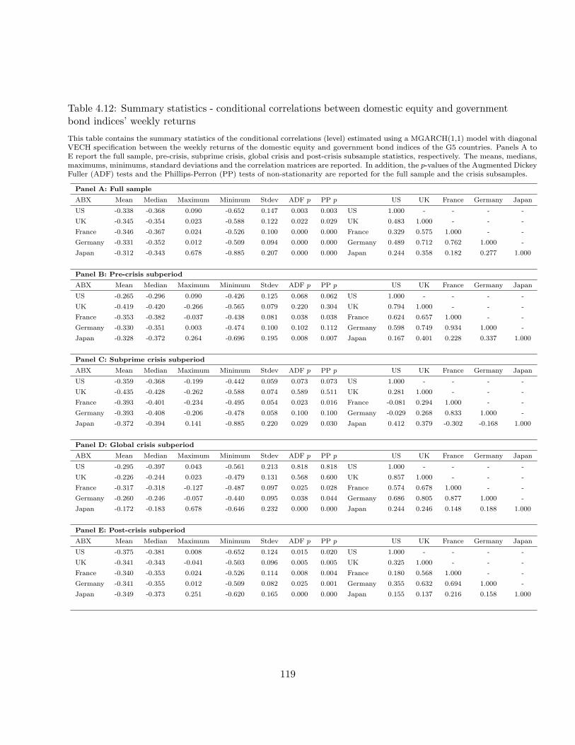
Table 4.12: Summary statistics - conditional correlations between domestic equity and governmentbond indices’ weekly returns
This table contains the summary statistics of the conditional correlations (level) estimated using a MGARCH(1,1) model with diagonalVECH specification between the weekly returns of the domestic equity and government bond indices of the G5 countries. Panels A toE report the full sample, pre-crisis, subprime crisis, global crisis and post-crisis subsample statistics, respectively. The means, medians,maximums, minimums, standard deviations and the correlation matrices are reported. In addition, the p-values of the Augmented DickeyFuller (ADF) tests and the Phillips-Perron (PP) tests of non-stationarity are reported for the full sample and the crisis subsamples.
Panel A: Full sample
ABX Mean Median Maximum Minimum Stdev ADF p PP p US UK France Germany Japan
US -0.338 -0.368 0.090 -0.652 0.147 0.003 0.003 US 1.000 - - - -
UK -0.345 -0.354 0.023 -0.588 0.122 0.022 0.029 UK 0.483 1.000 - - -
France -0.346 -0.367 0.024 -0.526 0.100 0.000 0.000 France 0.329 0.575 1.000 - -
Germany -0.331 -0.352 0.012 -0.509 0.094 0.000 0.000 Germany 0.489 0.712 0.762 1.000 -
Japan -0.312 -0.343 0.678 -0.885 0.207 0.000 0.000 Japan 0.244 0.358 0.182 0.277 1.000
Panel B: Pre-crisis subperiod
ABX Mean Median Maximum Minimum Stdev ADF p PP p US UK France Germany Japan
US -0.265 -0.296 0.090 -0.426 0.125 0.068 0.062 US 1.000 - - - -
UK -0.419 -0.420 -0.266 -0.565 0.079 0.220 0.304 UK 0.794 1.000 - - -
France -0.353 -0.382 -0.037 -0.438 0.081 0.038 0.038 France 0.624 0.657 1.000 - -
Germany -0.330 -0.351 0.003 -0.474 0.100 0.102 0.112 Germany 0.598 0.749 0.934 1.000 -
Japan -0.328 -0.372 0.264 -0.696 0.195 0.008 0.007 Japan 0.167 0.401 0.228 0.337 1.000
Panel C: Subprime crisis subperiod
ABX Mean Median Maximum Minimum Stdev ADF p PP p US UK France Germany Japan
US -0.359 -0.368 -0.199 -0.442 0.059 0.073 0.073 US 1.000 - - - -
UK -0.435 -0.428 -0.262 -0.588 0.074 0.589 0.511 UK 0.281 1.000 - - -
France -0.393 -0.401 -0.234 -0.495 0.054 0.023 0.016 France -0.081 0.294 1.000 - -
Germany -0.393 -0.408 -0.206 -0.478 0.058 0.100 0.100 Germany -0.029 0.268 0.833 1.000 -
Japan -0.372 -0.394 0.141 -0.885 0.220 0.029 0.030 Japan 0.412 0.379 -0.302 -0.168 1.000
Panel D: Global crisis subperiod
ABX Mean Median Maximum Minimum Stdev ADF p PP p US UK France Germany Japan
US -0.295 -0.397 0.043 -0.561 0.213 0.818 0.818 US 1.000 - - - -
UK -0.226 -0.244 0.023 -0.479 0.131 0.568 0.600 UK 0.857 1.000 - - -
France -0.317 -0.318 -0.127 -0.487 0.097 0.025 0.028 France 0.574 0.678 1.000 - -
Germany -0.260 -0.246 -0.057 -0.440 0.095 0.038 0.044 Germany 0.686 0.805 0.877 1.000 -
Japan -0.172 -0.183 0.678 -0.646 0.232 0.000 0.000 Japan 0.244 0.246 0.148 0.188 1.000
Panel E: Post-crisis subperiod
ABX Mean Median Maximum Minimum Stdev ADF p PP p US UK France Germany Japan
US -0.375 -0.381 0.008 -0.652 0.124 0.015 0.020 US 1.000 - - - -
UK -0.341 -0.343 -0.041 -0.503 0.096 0.005 0.005 UK 0.325 1.000 - - -
France -0.340 -0.353 0.024 -0.526 0.114 0.008 0.004 France 0.180 0.568 1.000 - -
Germany -0.341 -0.355 0.012 -0.509 0.082 0.025 0.001 Germany 0.355 0.632 0.694 1.000 -
Japan -0.349 -0.373 0.251 -0.620 0.165 0.000 0.000 Japan 0.155 0.137 0.216 0.158 1.000
119
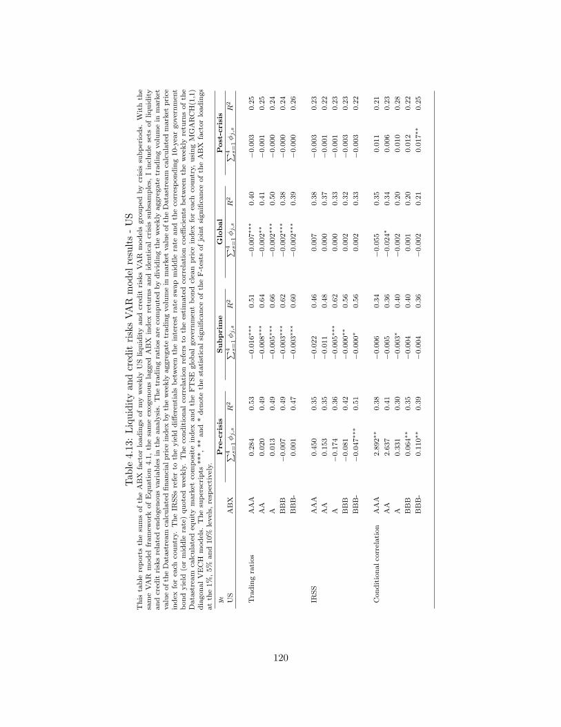
Tab
le4.13:Liquidityandcredit
risksVAR
model
results-US
This
table
reportsth
esu
msofth
eABX
factorloadingsofmyweekly
USliquidityandcred
itrisksVAR
modelsgrouped
bycrisis
subperiods.
Withth
esameVAR
model
framew
ork
ofEquation4.1,th
esameex
ogen
ouslagged
ABX
index
retu
rnsandiden
tica
lcrisis
subsamples,
Iincludesets
ofliquidity
andcred
itrisksrelateden
dogen
ousvariablesin
theanalysis.
Thetradingratiosare
computedbydividingth
eweekly
aggregate
tradingvolumein
market
valueofth
eDatastream
calculatedfinancialprice
index
byth
eweekly
aggregate
tradingvolumein
market
valueofth
eDatastream
calculatedmarket
price
index
forea
chco
untry.
TheIR
SSsreferto
theyield
differen
tials
betweenth
einterest
rate
swapmiddle
rate
andth
eco
rresponding10-yea
rgovernmen
tbondyield
(ormiddle
rate)quotedweekly.Theco
nditionalco
rrelationrefers
toth
eestimatedco
rrelationco
efficien
tsbetweenth
eweekly
retu
rnsofth
eDatastream
calculatedeq
uitymarket
composite
index
andth
eFTSE
globalgovernmen
tbondclea
nprice
index
forea
chco
untry,
usingMGARCH(1,1)
diagonalVECH
models.
Thesu
perscripts
***,**and*den
ote
thestatisticalsignifica
nce
ofth
eF-tests
ofjointsignifica
nce
ofth
eABX
factorloadings
atth
e1%,5%
and10%
levels,
resp
ectively.
yt
Pre-crisis
Subprim
eGlobal
Post-crisis
US
ABX
∑ 4 s=1ϕj,s
R2
∑ 4 s=1ϕj,s
R2
∑ 4 s=1ϕj,s
R2
∑ 4 s=1ϕj,s
R2
Tradingratios
AAA
0.284
0.53
−0.016∗∗
∗0.51
−0.007∗∗
∗0.40
−0.003
0.25
AA
0.020
0.49
−0.008∗∗
∗0.64
−0.002∗∗
0.41
−0.001
0.25
A0.013
0.49
−0.005∗∗
∗0.66
−0.002∗∗
∗0.50
−0.000
0.24
BBB
−0.007
0.49
−0.003∗∗
∗0.62
−0.002∗∗
∗0.38
−0.000
0.24
BBB-
0.001
0.47
−0.003∗∗
∗0.60
−0.002∗∗
∗0.39
−0.000
0.26
IRSS
AAA
0.450
0.35
−0.022
0.46
0.007
0.38
−0.003
0.23
AA
0.153
0.35
−0.011
0.48
0.000
0.37
−0.001
0.22
A−0.174
0.36
−0.005∗∗
∗0.62
0.000
0.33
−0.001
0.23
BBB
−0.081
0.42
−0.000∗∗
0.56
0.002
0.32
−0.003
0.23
BBB-
−0.047∗∗
∗0.51
−0.000∗
0.56
0.002
0.33
−0.003
0.22
Conditionalco
rrelation
AAA
2.892∗∗
0.38
−0.006
0.34
−0.055
0.35
0.011
0.21
AA
2.637
0.41
−0.005
0.36
−0.024∗
0.34
0.006
0.23
A0.331
0.30
−0.003∗
0.40
−0.002
0.20
0.010
0.28
BBB
0.064∗∗
0.35
−0.004
0.40
0.001
0.20
0.012
0.22
BBB-
0.110∗∗
0.39
−0.004
0.36
−0.002
0.21
0.017∗∗
0.25
120
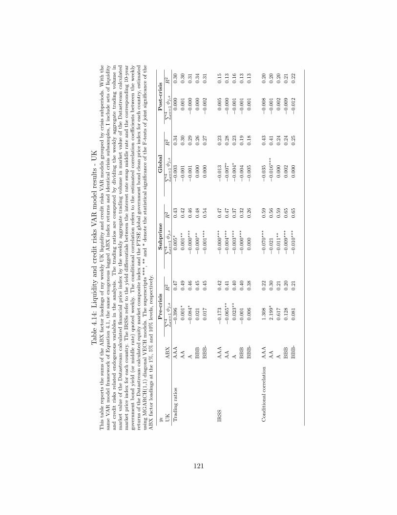
Tab
le4.14:LiquidityandcreditrisksVAR
model
results-UK
This
table
reportsth
esu
msofth
eABX
factorloadingsofmyweekly
UK
liquidityandcred
itrisksVAR
modelsgrouped
bycrisis
subperiods.
Withth
esameVAR
model
framew
ork
ofEquation4.1,th
esameex
ogen
ouslagged
ABX
index
retu
rnsandiden
tica
lcrisis
subsamples,
Iincludesets
ofliquidity
and
cred
itrisksrelated
endogen
ousvariablesin
theanalysis.
Thetradingratiosare
computed
by
dividingth
eweekly
aggregate
tradingvolumein
market
valueofth
eDatastream
calculatedfinancialprice
index
byth
eweekly
aggregate
tradingvolumein
market
valueofth
eDatastream
calculated
market
price
index
forea
chco
untry.
TheIR
SSsreferto
theyield
differen
tials
betweenth
einterest
rate
swapmiddle
rate
andth
eco
rresponding10-yea
rgovernmen
tbondyield
(ormiddle
rate)quotedweekly.Theco
nditionalco
rrelationrefers
toth
eestimatedco
rrelationco
efficien
tsbetweenth
eweekly
retu
rnsofth
eDatastream
calculatedeq
uitymarket
composite
index
andth
eFTSE
globalgovernmen
tbondclea
nprice
index
forea
chco
untry,
estimated
usingMGARCH(1,1)diagonalVECH
models.
Thesu
perscripts
***,**and*den
ote
thestatisticalsignifica
nce
ofth
eF-tests
ofjointsignifica
nce
ofth
eABX
factorloadingsatth
e1%,5%
and10%
levels,
resp
ectively.
yt
Pre-crisis
Subprim
eGlobal
Post-crisis
UK
ABX
∑ 4 s=1ϕj,s
R2
∑ 4 s=1ϕj,s
R2
∑ 4 s=1ϕj,s
R2
∑ 4 s=1ϕj,s
R2
Tradingratios
AAA
−0.396
0.47
0.005∗
0.43
−0.003
0.34
0.000
0.30
AA
0.001∗
0.49
0.001∗∗
0.42
−0.001
0.30
0.001
0.30
A−0.084∗
0.46
−0.000∗∗
∗0.46
−0.001
0.29
−0.000
0.31
BBB
0.021
0.45
−0.000∗∗
0.48
0.000
0.26
0.000
0.34
BBB-
0.017
0.45
−0.001∗∗
∗0.54
0.000
0.27
−0.002
0.31
IRSS
AAA
−0.173
0.42
−0.000∗∗
∗0.47
−0.013
0.23
0.005
0.15
AA
−0.065∗∗
0.41
−0.004∗∗
∗0.47
−0.007∗
0.28
−0.000
0.13
A0.023∗∗
0.40
−0.003∗∗
∗0.37
−0.004∗
0.23
−0.001
0.16
BBB
−0.001
0.40
−0.000∗∗
∗0.32
−0.004
0.19
−0.001
0.13
BBB-
0.006
0.38
0.000
0.26
−0.005
0.18
0.001
0.13
Conditionalco
rrelation
AAA
1.308
0.22
−0.070∗∗
∗0.59
−0.035
0.43
−0.008
0.20
AA
2.199∗
0.30
−0.021
0.56
−0.016∗∗
∗0.41
−0.001
0.20
A0.617
0.21
−0.011∗∗
0.59
0.000
0.24
0.002
0.20
BBB
0.128
0.20
−0.009∗∗
∗0.65
0.002
0.24
−0.009
0.21
BBB-
0.081
0.21
−0.010∗∗
∗0.65
0.000
0.25
−0.012
0.22
121
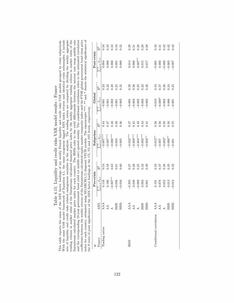
Tab
le4.15:LiquidityandcreditrisksVAR
model
results-France
This
table
reportsth
esu
msofth
eABX
factorloadingsofmyweekly
French
liquidityand
cred
itrisksVAR
modelsgrouped
bycrisis
subperiods.
With
thesameVAR
model
framew
ork
ofEquation
4.1,th
esameex
ogen
ouslagged
ABX
index
retu
rnsand
iden
tica
lcrisis
subsamples,
Iinclude
sets
ofliquidity
and
cred
itrisksrelated
endogen
ousvariablesin
theanalysis.
Thetradingratiosare
computed
by
dividingth
eweekly
aggregate
tradingvolumein
market
valueofth
eDatastream
calculated
financialprice
index
byth
eweekly
aggregate
tradingvolumein
market
valueofth
eDatastream
calculated
market
price
index
forea
chco
untry.
TheIR
SSsreferto
theyield
differen
tials
between
theinterest
rate
swap
middle
rate
andth
eco
rresponding10-yea
rgovernmen
tbondyield
(ormiddle
rate)quotedweekly.Theco
nditionalco
rrelationrefers
toth
eestimatedco
rrelation
coeffi
cien
tsbetweenth
eweekly
retu
rnsofth
eDatastream
calculatedeq
uitymarket
composite
index
andth
eFTSE
globalgovernmen
tbondclea
nprice
index
forea
chco
untry,
estimatedusingMGARCH(1,1)diagonalVECH
models.
Thesu
perscripts
***,**and*den
ote
thestatisticalsignifica
nce
of
theF-tests
ofjointsignifica
nce
ofth
eABX
factorloadingsatth
e1%,5%
and10%
levels,
resp
ectively.
yt
Pre-crisis
Subprim
eGlobal
Post-crisis
France
ABX
∑ 4 s=1ϕj,s
R2
∑ 4 s=1ϕj,s
R2
∑ 4 s=1ϕj,s
R2
∑ 4 s=1ϕj,s
R2
Tradingratios
AAA
0.116
0.54
−0.007∗∗
∗0.44
−0.001
0.23
0.004
0.34
AA
0.186
0.58
−0.007∗∗
∗0.47
−0.001
0.22
0.000
0.33
A−0.007∗∗
0.63
−0.006∗∗
∗0.46
−0.002
0.28
0.000
0.33
BBB
−0.056
0.61
−0.003
0.38
−0.001
0.25
0.001
0.34
BBB-
−0.034
0.60
−0.003
0.36
−0.002
0.25
0.000
0.32
IRSS
AAA
−0.393
0.27
−0.023∗∗
∗0.47
−0.005
0.39
0.014
0.28
AA
0.039
0.20
−0.009∗∗
∗0.45
−0.003
0.36
0.006
0.31
A−0.009
0.25
−0.004∗∗
∗0.49
−0.002
0.25
0.007∗∗
0.28
BBB
0.002
0.32
−0.002∗∗
∗0.43
−0.002
0.22
0.015
0.28
BBB-
0.001
0.30
−0.002∗∗
0.41
−0.002
0.26
0.017
0.29
Conditionalco
rrelation
AAA
0.191
0.33
−0.012∗∗
0.56
−0.019
0.34
−0.005
0.42
AA
0.878
0.37
−0.007
0.56
−0.009∗
0.37
0.000
0.41
A0.652
0.38
−0.002∗
0.56
−0.002
0.26
−0.000
0.42
BBB
0.013
0.35
−0.000∗∗
0.56
0.000
0.24
−0.005
0.42
BBB-
−0.012
0.32
−0.001
0.55
−0.001
0.25
−0.007
0.42
122
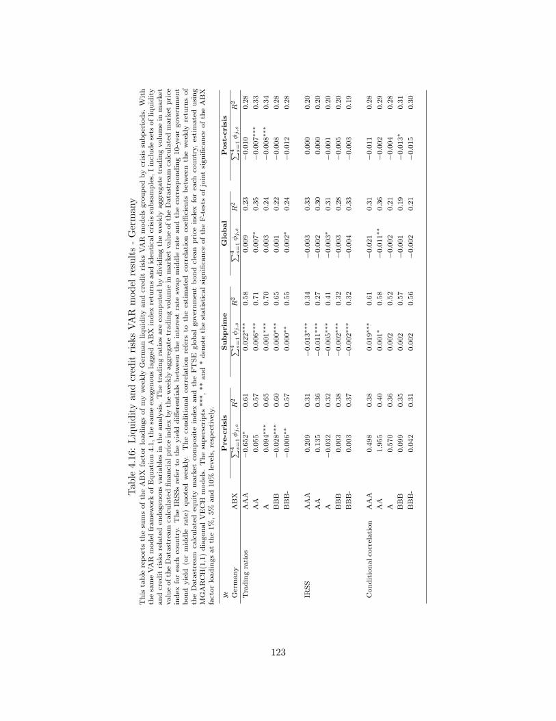
Tab
le4.16:Liquidityandcredit
risksVAR
model
results-Germany
This
table
reportsth
esu
msofth
eABX
factorloadingsofmyweekly
Germanliquidityandcred
itrisksVAR
modelsgrouped
bycrisis
subperiods.
With
thesameVAR
model
framew
ork
ofEquation4.1,th
esameex
ogen
ouslagged
ABX
index
retu
rnsandiden
tica
lcrisis
subsamples,
Iincludesets
ofliquidity
andcred
itrisksrelateden
dogen
ousvariablesin
theanalysis.
Thetradingratiosare
computedbydividingth
eweekly
aggregate
tradingvolumein
market
valueofth
eDatastream
calculatedfinancialprice
index
byth
eweekly
aggregate
tradingvolumein
market
valueofth
eDatastream
calculatedmarket
price
index
forea
chco
untry.
TheIR
SSsreferto
theyield
differen
tials
betweenth
einterest
rate
swapmiddle
rate
andth
eco
rresponding10-yea
rgovernmen
tbond
yield
(ormiddle
rate)quoted
weekly.
Theco
nditionalco
rrelation
refers
toth
eestimated
correlation
coeffi
cien
tsbetween
theweekly
retu
rnsof
theDatastream
calculated
equitymarket
composite
index
and
theFTSE
globalgovernmen
tbond
clea
nprice
index
forea
chco
untry,
estimated
using
MGARCH(1,1)diagonalVECH
models.
Thesu
perscripts
***,**and*den
ote
thestatisticalsignifica
nce
ofth
eF-tests
ofjointsignifica
nce
ofth
eABX
factorloadingsatth
e1%,5%
and10%
levels,
resp
ectively.
yt
Pre-crisis
Subprim
eGlobal
Post-crisis
Germany
ABX
∑ 4 s=1ϕj,s
R2
∑ 4 s=1ϕj,s
R2
∑ 4 s=1ϕj,s
R2
∑ 4 s=1ϕj,s
R2
Tradingratios
AAA
−0.652∗
0.61
0.022∗∗
∗0.58
0.009
0.23
−0.010
0.28
AA
0.055
0.57
0.006∗∗
∗0.71
0.007∗
0.35
−0.007∗∗
∗0.33
A0.094∗∗
∗0.65
0.001∗∗
∗0.70
0.003
0.24
−0.008∗∗
∗0.34
BBB
−0.028∗∗
∗0.60
0.000∗∗
∗0.65
0.001
0.22
−0.008
0.28
BBB-
−0.006∗∗
0.57
0.000∗∗
0.55
0.002∗
0.24
−0.012
0.28
IRSS
AAA
0.209
0.31
−0.013∗∗
∗0.34
−0.003
0.33
0.000
0.20
AA
0.135
0.36
−0.011∗∗
∗0.27
−0.002
0.30
0.000
0.20
A−0.032
0.32
−0.005∗∗
∗0.41
−0.003∗
0.31
−0.001
0.20
BBB
0.003
0.38
−0.002∗∗
∗0.32
−0.003
0.28
−0.005
0.20
BBB-
0.003
0.37
−0.002∗∗
∗0.32
−0.004
0.33
−0.003
0.19
Conditionalco
rrelation
AAA
0.498
0.38
0.019∗∗
∗0.61
−0.021
0.31
−0.011
0.28
AA
1.955
0.40
0.001∗
0.58
−0.011∗∗
0.36
−0.002
0.29
A0.570
0.36
0.002
0.52
−0.002
0.21
−0.004
0.28
BBB
0.099
0.35
0.002
0.57
−0.001
0.19
−0.013∗
0.31
BBB-
0.042
0.31
0.002
0.56
−0.002
0.21
−0.015
0.30
123
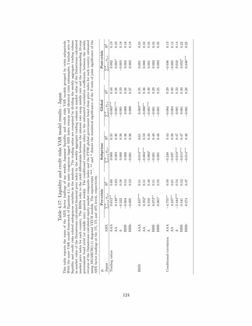
Tab
le4.17:LiquidityandcreditrisksVAR
model
results-Japan
This
table
reportsth
esu
msofth
eABX
factorloadingsofmy
weekly
Japaneseliquidity
and
cred
itrisksVAR
modelsgrouped
by
crisis
subperiods.
Withth
esameVAR
model
framew
ork
ofEquation4.1,th
esameex
ogen
ouslagged
ABX
index
retu
rnsandiden
tica
lcrisis
subsamples,
Iincludesets
of
liquidityandcred
itrisksrelateden
dogen
ousvariablesin
theanalysis.
Thetradingratiosare
computedbydividingth
eweekly
aggregate
tradingvolume
inmarket
valueofth
eDatastream
calculatedfinancialprice
index
byth
eweekly
aggregate
tradingvolumein
market
valueofth
eDatastream
calculated
market
price
index
forea
chco
untry.
TheIR
SSsreferto
theyield
differen
tials
betweenth
einterest
rate
swapmiddle
rate
andth
eco
rresponding10-yea
rgovernmen
tbond
yield
(ormiddle
rate)quoted
weekly.Theco
nditionalco
rrelation
refers
toth
eestimated
correlation
coeffi
cien
tsbetween
theweekly
retu
rnsofth
eDatastream
calculatedeq
uitymarket
composite
index
andth
eFTSE
globalgovernmen
tbondclea
nprice
index
forea
chco
untry,
estimated
usingMGARCH(1,1)diagonalVECH
models.
Thesu
perscripts
***,**and*den
ote
thestatisticalsignifica
nce
ofth
eF-tests
ofjointsignifica
nce
ofth
eABX
factorloadingsatth
e1%,5%
and10%
levels,
resp
ectively.
yt
Pre-crisis
Subprim
eGlobal
Post-crisis
Japan
ABX
∑ 4 s=1ϕj,s
R2
∑ 4 s=1ϕj,s
R2
∑ 4 s=1ϕj,s
R2
∑ 4 s=1ϕj,s
R2
Tradingratios
AAA
0.612∗∗
0.60
0.000
0.35
−0.003∗∗
∗0.44
0.002
0.19
AA
0.149∗∗
0.63
0.003
0.36
−0.001∗∗
∗0.38
0.001∗
0.23
A−0.222
0.58
0.000
0.38
−0.001
0.33
−0.003
0.18
BBB
−0.004
0.53
0.000
0.36
0.000
0.26
0.002
0.16
BBB-
−0.005
0.53
−0.001
0.36
0.000
0.27
0.003
0.18
IRSS
AAA
0.837∗∗
∗0.51
−0.013∗∗
∗0.61
0.003∗∗
∗0.35
0.001
0.33
AA
0.352∗
0.51
−0.004∗∗
∗0.59
−0.000∗∗
0.36
0.000
0.33
A0.310
0.48
−0.002∗
0.49
−0.001∗∗
∗0.39
0.001
0.34
BBB
0.073∗∗
0.51
−0.001
0.48
−0.001
0.29
0.002
0.34
BBB-
0.061∗
0.55
−0.001
0.48
−0.001
0.25
0.003
0.35
Conditionalco
rrelation
AAA
−4.755∗∗
0.50
−0.248
0.44
−0.004
0.29
−0.036
0.13
AA
4.237∗∗
0.61
−0.037
0.38
−0.004
0.30
−0.005
0.12
A−2.444∗∗
∗0.54
−0.019∗∗
∗0.47
0.001
0.33
0.010
0.14
BBB
0.541
0.52
−0.015∗∗
∗0.47
0.001
0.30
0.052∗
0.22
BBB-
0.274
0.47
−0.014∗∗
∗0.46
−0.001
0.28
0.048∗∗
∗0.25
124
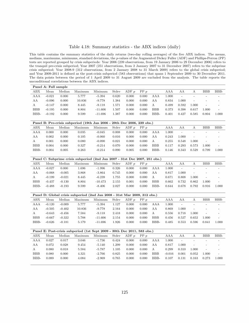
Table 4.18: Summary statistics - the ABX indices (daily)
This table contains the summary statistics of the daily returns (two-day rolling averages) of the five ABX indices. The means,medians, maximums, minimums, standard deviations, the p-values of the Augmented Dickey Fuller (ADF) and Phillips-Perron (PP)tests are reported grouped by crisis subperiods: Year 2006 (239 observations, from 19 January 2006 to 29 December 2006) refers tothe tranquil pre-crisis subperiod; Year 2007 (251 observations, from 2 January 2007 to 31 December 2007) refers to the subprimecrisis subperiod; Year 2008-9 (312 observations, from 2 January 2008 to 31 March 2009) refers to the global crisis subperiod;and Year 2009-2011 is defined as the post-crisis subperiod (583 observations) that spans 1 September 2009 to 30 December 2011.The data points between the period of 1 April 2009 to 31 August 2009 are excluded from the analysis. The table reports theunconditional correlations between the ABX indices.
Panel A: Full sample
ABX Mean Median Maximum Minimum Stdev ADF p PP p AAA AA A BBB BBB-
AAA -0.021 0.000 5.777 -5.394 0.620 0.000 0.000 AAA 1.000 - - - -
AA -0.096 0.000 10.836 -9.778 1.384 0.000 0.000 AA 0.834 1.000 - - -
A -0.147 0.000 8.445 -9.118 1.571 0.000 0.000 A 0.499 0.592 1.000 - -
BBB -0.195 0.000 8.804 -11.606 1.507 0.000 0.000 BBB 0.373 0.398 0.617 1.000 -
BBB- -0.192 0.000 9.599 -11.696 1.387 0.000 0.000 BBB- 0.401 0.427 0.585 0.804 1.000
Panel B: Pre-crisis subperiod (19th Jan 2006 - 29th Dec 2006, 239 obs.)
ABX Mean Median Maximum Minimum Stdev ADF p PP p AAA AA A BBB BBB-
AAA 0.000 0.000 0.035 -0.045 0.008 0.000 0.000 AAA 1.000 - - - -
AA 0.002 0.000 0.105 -0.060 0.016 0.000 0.000 AA 0.243 1.000 - - -
A 0.001 0.000 0.080 -0.090 0.021 0.000 0.000 A 0.255 0.548 1.000 - -
BBB 0.004 0.000 0.327 -0.214 0.070 0.000 0.000 BBB 0.117 0.293 0.573 1.000 -
BBB- 0.004 0.005 0.263 -0.214 0.090 0.005 0.000 BBB- 0.146 0.343 0.529 0.799 1.000
Panel C: Subprime crisis subperiod (2nd Jan 2007 - 31st Dec 2007, 251 obs.)
ABX Mean Median Maximum Minimum Stdev ADF p PP p AAA AA A BBB BBB-
AAA -0.027 0.000 1.696 -1.996 0.326 0.000 0.000 AAA 1.000 - - - -
AA -0.068 -0.005 3.868 -3.864 0.745 0.000 0.000 AA 0.817 1.000 - - -
A -0.199 -0.021 8.445 -6.239 1.755 0.000 0.000 A 0.671 0.808 1.000 - -
BBB -0.437 -0.130 8.804 -10.473 2.155 0.001 0.000 BBB 0.662 0.732 0.862 1.000 -
BBB- -0.488 -0.193 9.599 -8.406 2.027 0.000 0.000 BBB- 0.644 0.678 0.792 0.916 1.000
Panel D: Global crisis subperiod (2nd Jan 2008 - 31st Mar 2009, 312 obs.)
ABX Mean Median Maximum Minimum Stdev ADF p PP p AAA AA A BBB BBB-
AAA -0.120 -0.009 5.777 -5.394 1.127 0.000 0.000 AAA 1.000 - - - -
AA -0.505 -0.402 10.836 -9.778 2.164 0.000 0.000 AA 0.869 1.000 - - -
A -0.643 -0.456 7.584 -9.118 2.418 0.000 0.000 A 0.556 0.718 1.000 - -
BBB -0.667 -0.322 5.788 -11.606 2.154 0.000 0.000 BBB 0.456 0.527 0.652 1.000 -
BBB- -0.626 -0.181 5.179 -11.696 1.926 0.000 0.000 BBB- 0.485 0.553 0.596 0.841 1.000
Panel E: Post-crisis subperiod (1st Sept 2009 - 30th Dec 2011, 583 obs.)
ABX Mean Median Maximum Minimum Stdev ADF p PP p AAA AA A BBB BBB-
AAA 0.027 0.017 3.046 -1.736 0.424 0.000 0.000 AAA 1.000 - - - -
AA 0.072 0.028 9.454 -5.140 1.299 0.000 0.000 AA 0.817 1.000 - - -
A 0.080 0.018 5.584 -5.787 1.105 0.000 0.000 A 0.299 0.310 1.000 - -
BBB 0.080 0.000 4.321 -2.766 0.825 0.000 0.000 BBB -0.016 0.001 0.052 1.000 -
BBB- 0.089 0.000 4.084 -2.969 0.765 0.000 0.000 BBB- 0.107 0.131 0.163 0.273 1.000
125
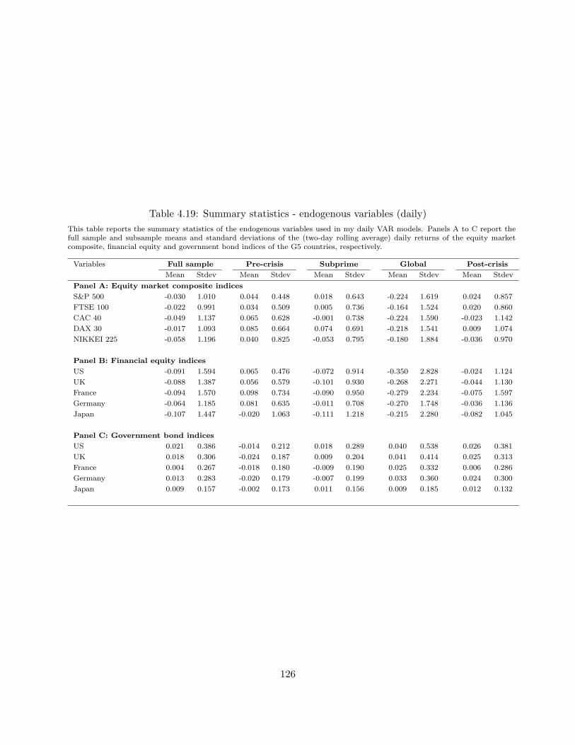
Table 4.19: Summary statistics - endogenous variables (daily)
This table reports the summary statistics of the endogenous variables used in my daily VAR models. Panels A to C report thefull sample and subsample means and standard deviations of the (two-day rolling average) daily returns of the equity marketcomposite, financial equity and government bond indices of the G5 countries, respectively.
Variables Full sample Pre-crisis Subprime Global Post-crisis
Mean Stdev Mean Stdev Mean Stdev Mean Stdev Mean Stdev
Panel A: Equity market composite indices
S&P 500 -0.030 1.010 0.044 0.448 0.018 0.643 -0.224 1.619 0.024 0.857
FTSE 100 -0.022 0.991 0.034 0.509 0.005 0.736 -0.164 1.524 0.020 0.860
CAC 40 -0.049 1.137 0.065 0.628 -0.001 0.738 -0.224 1.590 -0.023 1.142
DAX 30 -0.017 1.093 0.085 0.664 0.074 0.691 -0.218 1.541 0.009 1.074
NIKKEI 225 -0.058 1.196 0.040 0.825 -0.053 0.795 -0.180 1.884 -0.036 0.970
Panel B: Financial equity indices
US -0.091 1.594 0.065 0.476 -0.072 0.914 -0.350 2.828 -0.024 1.124
UK -0.088 1.387 0.056 0.579 -0.101 0.930 -0.268 2.271 -0.044 1.130
France -0.094 1.570 0.098 0.734 -0.090 0.950 -0.279 2.234 -0.075 1.597
Germany -0.064 1.185 0.081 0.635 -0.011 0.708 -0.270 1.748 -0.036 1.136
Japan -0.107 1.447 -0.020 1.063 -0.111 1.218 -0.215 2.280 -0.082 1.045
Panel C: Government bond indices
US 0.021 0.386 -0.014 0.212 0.018 0.289 0.040 0.538 0.026 0.381
UK 0.018 0.306 -0.024 0.187 0.009 0.204 0.041 0.414 0.025 0.313
France 0.004 0.267 -0.018 0.180 -0.009 0.190 0.025 0.332 0.006 0.286
Germany 0.013 0.283 -0.020 0.179 -0.007 0.199 0.033 0.360 0.024 0.300
Japan 0.009 0.157 -0.002 0.173 0.011 0.156 0.009 0.185 0.012 0.132
126
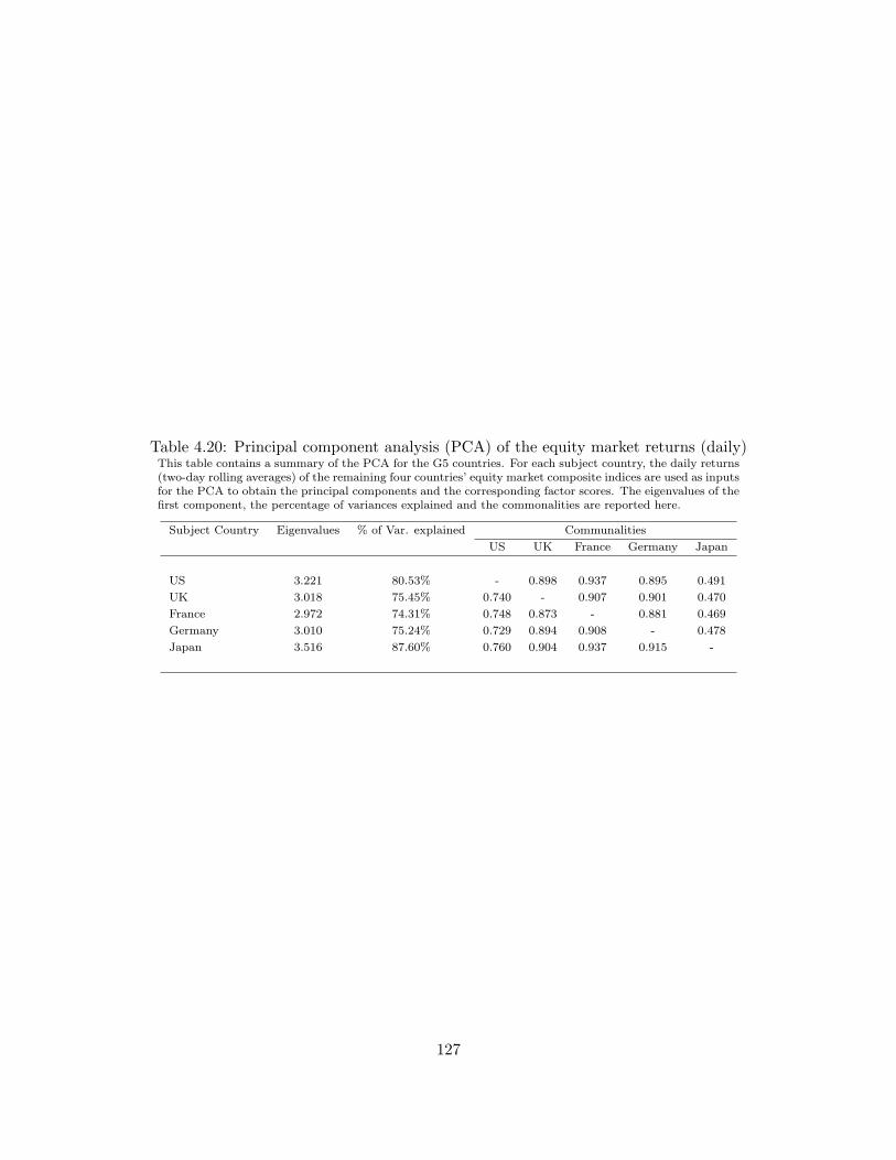
Table 4.20: Principal component analysis (PCA) of the equity market returns (daily)This table contains a summary of the PCA for the G5 countries. For each subject country, the daily returns(two-day rolling averages) of the remaining four countries’ equity market composite indices are used as inputsfor the PCA to obtain the principal components and the corresponding factor scores. The eigenvalues of thefirst component, the percentage of variances explained and the commonalities are reported here.
Subject Country Eigenvalues % of Var. explained Communalities
US UK France Germany Japan
US 3.221 80.53% - 0.898 0.937 0.895 0.491
UK 3.018 75.45% 0.740 - 0.907 0.901 0.470
France 2.972 74.31% 0.748 0.873 - 0.881 0.469
Germany 3.010 75.24% 0.729 0.894 0.908 - 0.478
Japan 3.516 87.60% 0.760 0.904 0.937 0.915 -
127
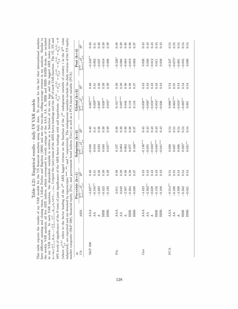
Table
4.21:Empiricalresults-dailyUSVAR
models
This
table
reportsth
eresu
ltsofmy
VAR
modelsforth
eUS
financialmarketsusing
daily
data.
To
accountforth
efact
thatintern
ationalmarkets
havedifferen
topen
ingand
closingtimes,Ifollow
Forb
esand
Rigobon
(2002)and
use
thetw
o-day
rolling-averageretu
rnsin
my
analysis.
Sim
ilarto
theweekly
VAR
analysis,
all
fiveABX
indices,which
correspond
tocred
itratingsofth
eAAA,AA,A,BBB
and
BBB-RMBS
dea
ls,are
included
inmy
VAR
models.
Inea
chVAR
equation,th
edep
enden
tvariable
iswritten
asa
function
ofitsown
lagsand
the
lagged
ABX
index
retu
rns:
yt=α
0+∑ 5 s
=1βsyt−
s+∑ 4 k
=1
∑ 5 s=
1ϕ
s,k
dkABX
t−
s+ϵt.Ireport
the(n
et)su
msofth
eABX
factorloadingsandth
eR
2ofea
chVAR
function.The1%,5%
and
10%
levelsofsignifica
nce
ofth
eF-tests
ofjointsignifica
nce
ofth
eABX
factorloadingswithnullhypoth
esis:ϕ(i,k
)j,1
=ϕ(i,k
)j,2
=ϕ(i,k
)j,3
=ϕ(i,k
)j,4
=ϕ(i,k
)j,5
=0
(whereϕ(i,k
)j,s
refers
toth
efactorloadingofth
est
hABX
lagged
retu
rnson
thefunction
ofth
ejt
hen
dogen
ousvariable
ofco
untry
iin
thekth
crisis
subperiod),
are
reported
andare
den
otedbysu
perscripts
***,**,and*,resp
ectively.
Theen
dogen
ousvariablesincludeth
edailyretu
rnsofth
eUSeq
uity
market
composite
(S&P
500),
financialeq
uity(F
in),
andgovernmen
tbondindices
(Gov)aswellasaPCA
latentvariable
(PCA).
yt
Pre-crisis
(k=1)
Subprim
e(k
=2)
Global(k
=3)
Post
(k=4)
US
ABX
∑ 5 s=1ϕk j,s
R2
∑ 5 s=1ϕk j,s
R2
∑ 5 s=1ϕk j,s
R2
∑ 5 s=1ϕk j,s
R2
S&P
500
AAA
−3.827∗∗
0.40
−0.048
0.40
0.067∗∗
∗0.40
−0.242∗∗
0.40
AA
−0.194∗∗
0.41
0.010
0.41
0.029∗∗
∗0.41
−0.062
0.41
A−2.882
0.38
0.023
0.38
−0.007
0.38
−0.037
0.38
BBB
−0.423
0.39
0.040
0.39
0.038∗∗
0.39
−0.018
0.39
BBB-
−0.192
0.39
0.047∗∗
0.39
0.035∗
0.39
−0.006
0.39
Fin
AAA
2.011
0.39
0.107
0.39
0.191∗∗
∗0.39
−0.326∗
0.39
AA
0.649
0.39
0.063
0.39
0.097∗∗
∗0.39
−0.086
0.39
A−2.567
0.36
0.062
0.36
0.046
0.36
−0.064
0.36
BBB
−0.304
0.38
0.077
0.38
0.119
0.38
−0.019
0.38
BBB-
−0.039
0.37
0.100∗∗
0.37
0.116
0.37
−0.002
0.37
Gov
AAA
−4.423
0.43
−0.136∗∗
∗0.43
−0.038∗∗
0.43
0.026
0.43
AA
−2.562∗∗
0.43
−0.035
0.43
−0.026∗
0.43
0.020
0.43
A−0.629
0.43
−0.033∗∗
0.43
−0.010∗∗
∗0.43
−0.012
0.43
BBB
−0.150
0.43
−0.040∗∗
∗0.43
−0.034∗
0.43
0.011
0.43
BBB-
−0.169
0.43
−0.041∗∗
∗0.43
−0.036
0.43
0.038
0.43
PCA
AAA
−9.514∗∗
0.54
0.036
0.54
0.000∗∗
0.54
−0.247
0.54
AA
−0.100
0.55
0.037
0.55
0.004∗∗
∗0.55
−0.075∗
0.55
A−4.509
0.54
0.036
0.54
−0.016∗
0.54
−0.001
0.54
BBB
−0.562
0.54
0.025∗
0.54
−0.005∗∗
0.54
−0.045
0.54
BBB-
−0.021
0.54
0.021∗∗
0.54
0.001
0.54
0.000
0.54
128
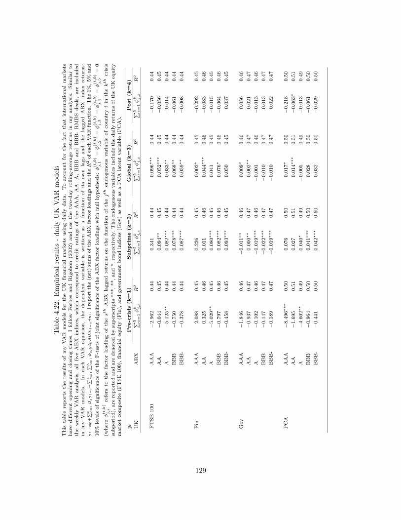
Table
4.22:Empiricalresults-dailyUK
VAR
models
This
table
reportsth
eresu
ltsofmy
VAR
modelsforth
eUK
financialmarketsusingdaily
data.
Toaccountforth
efact
thatintern
ationalmarkets
havedifferen
topen
ingand
closingtimes,Ifollow
Forb
esand
Rigobon
(2002)and
use
thetw
o-day
rolling-averageretu
rnsin
my
analysis.
Sim
ilarto
theweekly
VAR
analysis,
all
fiveABX
indices,which
correspond
tocred
itratingsofth
eAAA,AA,A,BBB
and
BBB-RMBS
dea
ls,are
included
inmy
VAR
models.
Inea
chVAR
equation,th
edep
enden
tvariable
iswritten
asa
function
ofitsown
lagsand
the
lagged
ABX
index
retu
rns:
yt=α
0+∑ 5 s
=1βsyt−
i+∑ 4 k
=1
∑ 5 s=
1ϕ
s,k
dkABX
t−
s+ϵt.Ireport
the(n
et)su
msofth
eABX
factorloadingsandth
eR
2ofea
chVAR
function.The1%,5%
and
10%
levelsofsignifica
nce
ofth
eF-tests
ofjointsignifica
nce
ofth
eABX
factorloadingswithnullhypoth
esis:ϕ(i,k
)j,1
=ϕ(i,k
)j,2
=ϕ(i,k
)j,3
=ϕ(i,k
)j,4
=ϕ(i,k
)j,5
=0
(whereϕ(i,k
)j,s
refers
toth
efactorloadingofth
est
hABX
lagged
retu
rnson
thefunction
ofth
ejt
hen
dogen
ousvariable
ofco
untry
iin
thekth
crisis
subperiod),
are
reported
andare
den
otedbysu
perscripts
***,**,and*,resp
ectively.
Theen
dogen
ousvariablesincludeth
edailyretu
rnsofth
eUK
equity
market
composite
(FTSE
100),
financialeq
uity(F
in),
andgovernmen
tbondindices
(Gov)aswellasaPCA
latentvariable
(PCA).
yt
Pre-crisis
(k=1)
Subprim
e(k
=2)
Global(k
=3)
Post
(k=4)
UK
ABX
∑ 5 s=1ϕk j,s
R2
∑ 5 s=1ϕk j,s
R2
∑ 5 s=1ϕk j,s
R2
∑ 5 s=1ϕk j,s
R2
FTSE
100
AAA
−2.962
0.44
0.341
0.44
0.096∗∗
∗0.44
−0.170
0.44
AA
−0.044
0.45
0.094∗∗
0.45
0.052∗∗
∗0.45
−0.056
0.45
A−5.125∗∗
0.44
0.082∗∗
∗0.44
0.033∗∗
0.44
−0.014
0.44
BBB
−0.750
0.44
0.078∗∗
∗0.44
0.068∗∗
0.44
−0.061
0.44
BBB-
−0.378
0.44
0.087∗∗
∗0.44
0.059∗∗
0.44
−0.008
0.44
Fin
AAA
2.088
0.45
0.226
0.45
0.002∗
0.45
−0.292
0.45
AA
0.325
0.46
0.011
0.46
0.044∗∗
∗0.46
−0.083
0.46
A−5.029∗∗
0.45
0.080∗∗
∗0.45
0.041
0.45
−0.015
0.45
BBB
−0.797
0.46
0.082∗∗
∗0.46
0.076∗
0.46
−0.064
0.46
BBB-
−0.458
0.45
0.093∗∗
∗0.45
0.050
0.45
0.037
0.45
Gov
AAA
−1.846
0.46
−0.011∗∗
0.46
0.009∗
0.46
0.056
0.46
AA
−0.937
0.47
0.000∗∗
0.47
0.002∗∗
0.47
0.021
0.47
A−0.102
0.46
−0.019∗∗
∗0.46
−0.001
0.46
−0.013
0.46
BBB
−0.147
0.47
−0.022∗∗
∗0.47
−0.010
0.47
0.013
0.47
BBB-
−0.189
0.47
−0.019∗∗
∗0.47
−0.010
0.47
0.022
0.47
PCA
AAA
−8.496∗∗
∗0.50
0.076
0.50
0.017∗
0.50
−0.218
0.50
AA
−1.695
0.51
0.027
0.51
0.014∗∗
∗0.51
−0.063∗
0.51
A−4.602∗∗
0.49
0.040∗
0.49
−0.005
0.49
−0.013
0.49
BBB
−0.964
0.50
0.041∗∗
∗0.50
0.028
0.50
−0.061
0.50
BBB-
−0.441
0.50
0.042∗∗
∗0.50
0.032
0.50
−0.029
0.50
129
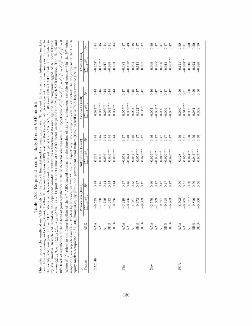
Table
4.23:Empiricalresults-dailyFrench
VAR
models
This
table
reportsth
eresu
ltsofmyVAR
modelsforth
eFrench
financialmarketsusingdailydata.Toaccountforth
efact
thatintern
ationalmarkets
havedifferen
topen
ingand
closingtimes,Ifollow
Forb
esand
Rigobon
(2002)and
use
thetw
o-dayrolling-averageretu
rnsformyanalysis.
Sim
ilarto
theweekly
VAR
analysis,
all
fiveABX
indices,which
correspond
tocred
itratingsofth
eAAA,AA,A,BBB
and
BBB-RMBS
dea
ls,are
included
inmyVAR
models.
Inea
chVAR
equation,th
edep
enden
tvariable
iswritten
asafunctionofitsownlagsandth
eex
ogen
ouslagged
ABX
index
retu
rns:
yt=α
0+∑ 5 s
=1βsyt−
i+∑ 4 k
=1
∑ 5 s=
1ϕ
s,k
dkABX
t−
s+ϵt.Ireport
the(n
et)su
msofth
eABX
factorloadingsandth
eR
2ofea
chVAR
function.The1%,5%
and
10%
levelsofsignifica
nce
ofth
eF-tests
ofjointsignifica
nce
ofth
eABX
factorloadingswithnullhypoth
esis:ϕ(i,k
)j,1
=ϕ(i,k
)j,2
=ϕ(i,k
)j,3
=ϕ(i,k
)j,4
=ϕ(i,k
)j,5
=0
(whereϕ(i,k
)j,s
refers
toth
efactorloadingofth
est
hABX
lagged
retu
rnson
thefunction
ofth
ejt
hen
dogen
ousvariable
ofco
untry
iin
thekth
crisis
subperiod),
are
reported
andare
den
otedbysu
perscripts
***,**,and*,resp
ectively.
Theen
dogen
ousvariablesincludeth
edailyretu
rnsofth
eFrench
equitymarket
composite
(CAC
40),
financialeq
uity(F
in),
andgovernmen
tbondindices
(Gov)aswellasaPCA
latentvariable
(PCA).
yt
Pre-crisis
(k=1)
Subprim
e(k
=2)
Global(k
=3)
Post
(k=4)
France
ABX
∑ 5 s=1ϕk j,s
R2
∑ 5 s=1ϕk j,s
R2
∑ 5 s=1ϕk j,s
R2
∑ 5 s=1ϕk j,s
R2
CAC
40
AAA
−6.555
0.44
0.223
0.44
0.082∗∗
0.44
−0.258∗
0.44
AA
−1.920
0.45
0.069
0.45
0.060∗∗
∗0.45
−0.102∗∗
0.45
A−4.719
0.44
0.056∗
0.44
0.050∗∗
0.44
−0.017
0.44
BBB
−1.032
0.44
0.046∗∗
∗0.44
0.083∗∗
∗0.44
−0.099
0.44
BBB-
−0.576
0.44
0.058∗∗
∗0.44
0.080∗∗
0.44
−0.003
0.44
Fin
AAA
−3.320
0.47
−0.058
0.47
0.057∗∗
0.47
−0.383
0.47
AA
−0.286
0.48
−0.024
0.48
0.082∗∗
∗0.48
−0.138∗
0.48
A−4.087
0.48
0.057∗∗
0.48
0.091∗
0.48
0.004
0.48
BBB
−0.472
0.47
0.058∗∗
∗0.47
0.122∗∗
0.47
−0.114
0.47
BBB-
−0.003
0.47
0.075∗∗
∗0.47
0.117∗
0.47
0.067
0.47
Gov
AAA
−2.570
0.46
−0.029∗∗
0.46
−0.004
0.46
0.049
0.46
AA
−1.509
0.47
−0.006∗∗
0.47
−0.001∗∗
0.47
0.025∗
0.47
A−0.527
0.47
−0.018∗∗
0.47
0.000
0.47
0.006
0.47
BBB
−0.315
0.47
−0.020∗∗
∗0.47
−0.009
0.47
0.013
0.47
BBB-
−0.263
0.47
−0.020∗∗
∗0.47
−0.007
0.47
0.031∗∗
∗0.47
PCA
AAA
−8.502∗∗
0.50
0.128
0.50
0.030∗
0.50
−0.171∗
0.50
AA
−0.905
0.51
0.050∗
0.51
0.019∗∗
∗0.51
−0.048∗∗
0.51
A−4.671∗∗
0.50
0.044∗∗
0.50
−0.002
0.50
−0.016
0.50
BBB
−0.816
0.50
0.043∗∗
∗0.50
0.034
0.50
−0.072
0.50
BBB-
−0.300
0.50
0.047∗∗
∗0.50
0.038
0.50
−0.026
0.50
130

Table
4.24:Empiricalresults-dailyGermanVAR
models
This
table
reportsth
eresu
ltsofmyVAR
modelsforth
eGerman
financialmarketsusingdailydata.
Toaccountforth
efact
thatintern
ationalmar-
ketshavedifferen
topen
ingand
closingtimes,Ifollow
Forb
esand
Rigobon
(2002)and
use
thetw
o-day
rolling-averageretu
rnsformy
analysis.
Sim
-ilarto
theweekly
VAR
analysis,
all
fiveABX
indices,which
correspond
tocred
itratingsofth
eAAA,AA,A,BBB
and
BBB-RMBS
dea
ls,are
included
inmyVAR
models.
Inea
chVAR
equation,th
edep
enden
tvariable
iswritten
asafunctionofitsownlagsandth
elagged
ABX
index
retu
rns:
yt=α
0+∑ 5 s
=1βsyt−
i+∑ 4 k
=1
∑ 5 s=
1ϕ
s,k
dkABX
t−
s+ϵt.Ireport
the(n
et)su
msofth
eABX
factorloadingsandth
eR
2ofea
chVAR
function.The1%,5%
and
10%
levelsofsignifica
nce
ofth
eF-tests
ofjointsignifica
nce
onth
eABX
factorloadingswithnullhypoth
esis:ϕ(i,k
)j,1
=ϕ(i,k
)j,2
=ϕ(i,k
)j,3
=ϕ(i,k
)j,4
=ϕ(i,k
)j,5
=0
(whereϕ(i,k
)j,s
refers
toth
efactorloadingofth
est
hABX
lagged
retu
rnson
thefunction
ofth
ejt
hen
dogen
ousvariable
ofco
untry
iin
thekth
crisis
subperiod),
are
reported
andare
den
otedbysu
perscripts
***,**,and*,resp
ectively.
Theen
dogen
ousvariablesincludeth
edailyretu
rnsofth
eGerman
equitymarket
composite
(DAX
30),
financialeq
uity(F
in),
andgovernmen
tbondindices
(Gov)aswellasaPCA
latentvariable
(PCA).
yt
Pre-crisis
(k=1)
Subprim
e(k
=2)
Global(k
=3)
Post
(k=4)
Germany
ABX
∑ 5 s=1ϕk j,s
R2
∑ 5 s=1ϕk j,s
R2
∑ 5 s=1ϕk j,s
R2
∑ 5 s=1ϕk j,s
R2
DAX
40
AAA
−11.776∗
0.44
0.208
0.44
0.103∗∗
∗0.44
−0.248∗∗
0.44
AA
−2.826
0.45
0.064∗∗
0.45
0.058∗∗
∗0.45
−0.083∗∗
0.45
A−6.298∗∗
0.44
0.053∗∗
∗0.44
0.022
0.44
−0.004
0.44
BBB
−1.304
0.44
0.045∗∗
∗0.44
0.055
0.44
−0.048
0.44
BBB-
−0.574
0.44
0.056∗∗
∗0.44
0.063
0.44
0.029
0.44
Fin
AAA
−1.659
0.48
0.006
0.48
0.004∗∗
0.48
−0.309
0.48
AA
0.457
0.48
−0.015
0.48
0.030∗∗
∗0.48
−0.100
0.48
A−2.962
0.47
0.045∗
0.47
0.032
0.47
0.007
0.47
BBB
−0.250
0.47
0.050∗∗
0.47
0.046∗∗
0.47
−0.055
0.47
BBB-
0.032
0.47
0.059∗∗
∗0.47
0.040
0.47
0.024
0.47
Gov
AAA
−2.409
0.48
−0.028
0.48
−0.011
0.48
0.070
0.48
AA
−1.665
0.49
−0.001∗∗
∗0.49
−0.005∗
0.49
0.031∗∗
0.49
A−0.526
0.48
−0.019∗∗
0.48
−0.002
0.48
−0.016
0.48
BBB
−0.302∗∗
0.49
−0.021∗∗
∗0.49
−0.011
0.49
0.010
0.49
BBB-
−0.261
0.49
−0.022∗∗
∗0.49
−0.011
0.49
0.018
0.49
PCA
AAA
−7.038∗∗
0.49
0.163
0.49
0.015
0.49
−0.226
0.49
AA
0.273
0.50
0.060
0.50
0.015∗∗
∗0.50
−0.058∗
0.50
A−3.862∗
0.49
0.056∗∗
0.49
−0.011
0.49
−0.017
0.49
BBB
−0.707
0.50
0.051∗∗
∗0.50
0.019
0.50
−0.068
0.50
BBB-
−0.184
0.49
0.052∗∗
∗0.49
0.026
0.49
−0.038
0.49
131
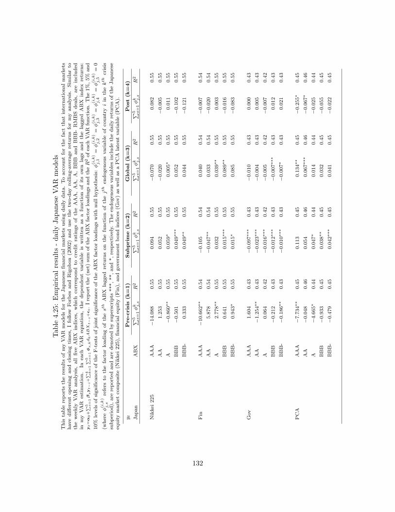
Table
4.25:Empiricalresults-dailyJapaneseVAR
models
This
table
reportsth
eresu
ltsofmyVAR
modelsforth
eJapanesefinancialmarketsusingdailydata.Toaccountforth
efact
thatintern
ationalmarkets
havedifferen
topen
ingand
closingtimes,Ifollow
Forb
esand
Rigobon
(2002)and
use
thetw
o-dayrolling-averageretu
rnsformyanalysis.
Sim
ilarto
theweekly
VAR
analysis,
all
fiveABX
indices,which
correspond
tocred
itratingsofth
eAAA,AA,A,BBB
and
BBB-RMBS
dea
ls,are
included
inmy
VAR
estimation.
Inea
chVAR
equation,th
edep
enden
tvariable
iswritten
asa
function
ofitsown
lagsand
thelagged
ABX
index
retu
rns:
yt=α
0+∑ 5 s
=1βsyt−
i+∑ 4 k
=1
∑ 5 s=
1ϕ
s,k
dkABX
t−
s+ϵt.Ireport
the(n
et)su
mofth
eABX
factorloadingsandth
eR
2ofea
chVAR
function.The1%,5%
and
10%
levelsofsignifica
nce
ofth
eF-tests
ofjointsignifica
nce
ofth
eABX
factorloadingswithnullhypoth
esis:ϕ(i,k
)j,1
=ϕ(i,k
)j,2
=ϕ(i,k
)j,3
=ϕ(i,k
)j,4
=ϕ(i,k
)j,5
=0
(whereϕ(i,k
)j,s
refers
toth
efactorloadingofth
est
hABX
lagged
retu
rnson
thefunction
ofth
ejt
hen
dogen
ousvariable
ofco
untry
iin
thekth
crisis
subperiod),
are
reported
andare
den
otedbysu
perscripts
***,**,and*,resp
ectively.
Theen
dogen
ousvariablesincludeth
edailyretu
rnsofth
eJapanese
equitymarket
composite
(Nikkei
225),
financialeq
uity(F
in),
andgovernmen
tbondindices
(Gov)aswellasaPCA
latentvariable
(PCA).
yt
Pre-crisis
(k=1)
Subprim
e(k
=2)
Global(k
=3)
Post
(k=4)
Japan
ABX
∑ 5 s=1ϕk j,s
R2
∑ 5 s=1ϕk j,s
R2
∑ 5 s=1ϕk j,s
R2
∑ 5 s=1ϕk j,s
R2
Nikkei
225
AAA
−14.088
0.55
0.094
0.55
−0.070
0.55
0.082
0.55
AA
1.253
0.55
0.052
0.55
−0.020
0.55
−0.005
0.55
A−0.860∗∗
0.55
0.059∗
0.55
0.005∗
0.55
0.011
0.55
BBB
−0.501
0.55
0.049∗∗
∗0.55
0.052
0.55
−0.102
0.55
BBB-
0.333
0.55
0.049∗∗
0.55
0.044
0.55
−0.121
0.55
Fin
AAA
−10.662∗∗
0.54
−0.105
0.54
0.040
0.54
−0.007
0.54
AA
5.878
0.54
−0.047∗∗
0.54
0.033
0.54
−0.020
0.54
A2.778∗∗
0.55
0.032
0.55
0.039∗∗
0.55
0.003
0.55
BBB
0.641
0.55
0.015∗∗
∗0.55
0.089∗∗
0.55
−0.016
0.55
BBB-
0.943∗
0.55
0.015∗
0.55
0.085
0.55
−0.083
0.55
Gov
AAA
1.604
0.43
−0.097∗∗
∗0.43
−0.010
0.43
0.000
0.43
AA
−1.254∗∗
0.43
−0.023∗∗
∗0.43
−0.004
0.43
0.005
0.43
A0.064
0.42
−0.016∗∗
∗0.42
−0.005
0.42
−0.007
0.42
BBB
−0.212
0.43
−0.012∗∗
∗0.43
−0.007∗∗
∗0.43
0.012
0.43
BBB-
−0.186∗∗
0.43
−0.010∗∗
∗0.43
−0.007∗
0.43
0.021
0.43
PCA
AAA
−7.734∗∗
0.45
0.113
0.45
0.134∗∗
0.45
−0.255∗
0.45
AA
−0.048
0.46
0.054
0.46
0.067∗∗
∗0.46
−0.067∗
0.46
A−4.665∗
0.44
0.047∗
0.44
0.014
0.44
−0.025
0.44
BBB
−0.933
0.45
0.038∗∗
0.45
0.032
0.45
−0.055
0.45
BBB-
−0.479
0.45
0.042∗∗
∗0.45
0.041
0.45
−0.022
0.45
132
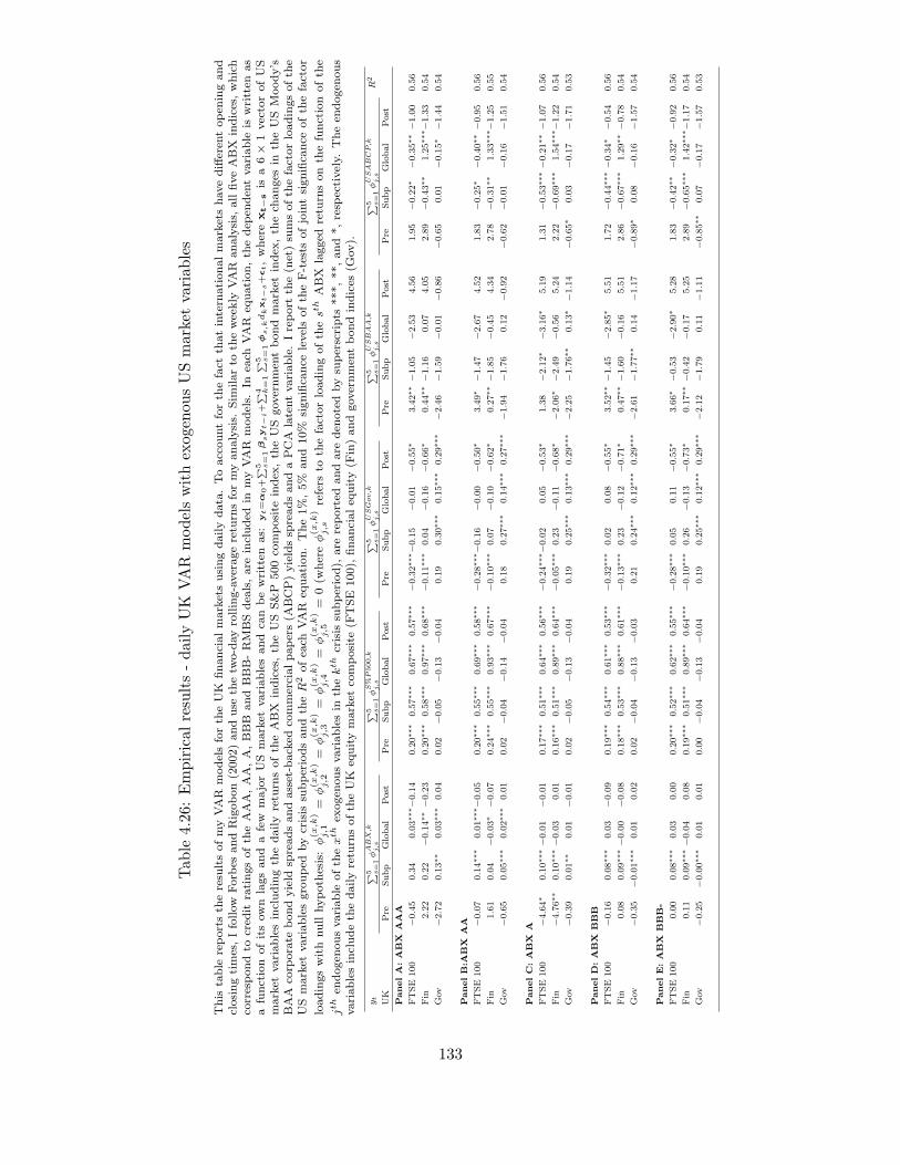
Tab
le4.26
:Empiricalresults-dailyUK
VAR
modelswithexogenousUSmarket
variables
This
table
reportsth
eresu
ltsofmyVAR
modelsforth
eUK
financialmarketsusingdailydata.Toaccountforth
efact
thatintern
ationalmarketshavedifferen
topen
ingand
closingtimes,Ifollow
Forb
esandRigobon(2002)anduse
thetw
o-dayrolling-averageretu
rnsformyanalysis.
Sim
ilarto
theweekly
VAR
analysis,
allfiveABX
indices,which
correspondto
cred
itratingsofth
eAAA,AA,A,BBB
andBBB-RMBSdea
ls,are
included
inmyVAR
models.
Inea
chVAR
equation,th
edep
enden
tvariable
iswritten
as
afunction
ofitsown
lagsand
afew
majorUS
market
variablesand
can
bewritten
as:
yt=α
0+∑ 5 s
=1βsyt−
i+∑ 4 k
=1
∑ 5 s=
1ϕ
s,k
dkxt−
s+ϵt,wherext−sis
a6×
1vectorofUS
market
variablesincludingth
edailyretu
rnsofth
eABX
indices,th
eUS
S&P
500co
mposite
index
,th
eUS
governmen
tbond
market
index
,th
ech
anges
inth
eUS
Moody’s
BAA
corp
orate
bondyield
spreadsandasset-backed
commercialpapers(A
BCP)yieldssp
readsandaPCA
latentvariable.Ireport
the(n
et)su
msofth
efactorloadingsofth
eUSmarket
variablesgrouped
bycrisis
subperiodsandth
eR
2ofea
chVAR
equation.The1%,5%
and10%
significa
nce
levelsofth
eF-tests
ofjointsignifica
nce
ofth
efactor
loadingswithnullhypoth
esis:ϕ(x
,k)
j,1
=ϕ(x
,k)
j,2
=ϕ(x
,k)
j,3
=ϕ(x
,k)
j,4
=ϕ(x
,k)
j,5
=0(w
hereϕ(x
,k)
j,s
refers
toth
efactorloadingofth
est
hABX
lagged
retu
rnsonth
efunctionofth
e
jthen
dogen
ousvariable
ofth
exth
exogen
ousvariablesin
thekth
crisis
subperiod),
are
reported
andare
den
otedbysu
perscripts
***,**,and*,resp
ectively.
Theen
dogen
ous
variablesincludeth
edailyretu
rnsofth
eUK
equitymarket
composite
(FTSE
100),
financialeq
uity(F
in)andgovernmen
tbondindices
(Gov).
yt
∑ 5 s=1ϕABX
,kj,s
∑ 5 s=1ϕS%P500,k
j,s
∑ 5 s=1ϕUSGov,k
j,s
∑ 5 s=1ϕUSBAA,k
j,s
∑ 5 s=1ϕUSABCP,k
j,s
R2
UK
Pre
Subp
Global
Post
Pre
Subp
Global
Post
Pre
Subp
Global
Post
Pre
Subp
Global
Post
Pre
Subp
Global
Post
PanelA:ABX
AAA
FTSE
100
−0.45
0.34
0.03∗∗
∗−0.14
0.20∗∗
∗0.57∗∗
∗0.67∗∗
∗0.57∗∗
∗−0.32∗∗
∗−0.15
−0.01
−0.55∗
3.42∗∗
−1.05
−2.53
4.56
1.95
−0.22∗
−0.35∗∗
−1.00
0.56
Fin
2.22
0.22
−0.14∗∗
−0.23
0.20∗∗
∗0.58∗∗
∗0.97∗∗
∗0.68∗∗
∗−0.11∗∗
∗0.04
−0.16
−0.66∗
0.44∗∗
−1.16
0.07
4.05
2.89
−0.43∗∗
1.25∗∗
∗−1.33
0.54
Gov
−2.72
0.13∗∗
0.03∗∗
∗0.04
0.02
−0.05
−0.13
−0.04
0.19
0.30∗∗
∗0.15∗∗
∗0.29∗∗
∗−2.46
−1.59
−0.01
−0.86
−0.65
0.01
−0.15∗
−1.44
0.54
PanelB:A
BX
AA
FTSE
100
−0.07
0.14∗∗
∗0.01∗∗
∗−0.05
0.20∗∗
∗0.55∗∗
∗0.69∗∗
∗0.58∗∗
∗−0.28∗∗
∗−0.16
−0.00
−0.50∗
3.49∗
−1.47
−2.67
4.52
1.83
−0.25∗
−0.40∗∗
−0.95
0.56
Fin
1.61
0.04
−0.03∗
−0.07
0.24∗∗
∗0.55∗∗
∗0.93∗∗
∗0.67∗∗
∗−0.10∗∗
∗0.07
−0.10
−0.62∗
0.27∗∗
−1.85
−0.45
4.34
2.78
−0.31∗∗
1.33∗∗
∗−1.25
0.55
Gov
−0.65
0.05∗∗
∗0.02∗∗
∗0.01
0.02
−0.04
−0.14
−0.04
0.18
0.27∗∗
∗0.14∗∗
∗0.27∗∗
∗−1.94
−1.76
0.12
−0.92
−0.62
−0.01
−0.16
−1.51
0.54
PanelC:ABX
A
FTSE
100
−4.64∗
0.10∗∗
∗−0.01
−0.01
0.17∗∗
∗0.51∗∗
∗0.64∗∗
∗0.56∗∗
∗−0.24∗∗
∗−0.02
0.05
−0.53∗
1.38
−2.12∗
−3.16∗
5.19
1.31
−0.53∗∗
∗−0.21∗∗
−1.07
0.56
Fin
−4.76∗∗
0.10∗∗
∗−0.03
0.01
0.16∗∗
∗0.51∗∗
∗0.89∗∗
∗0.64∗∗
∗−0.05∗∗
∗0.23
−0.11
−0.68∗
−2.06∗
−2.49
−0.56
5.24
2.22
−0.69∗∗
∗1.54∗∗
∗−1.22
0.54
Gov
−0.39
0.01∗∗
0.01
−0.01
0.02
−0.05
−0.13
−0.04
0.19
0.25∗∗
∗0.13∗∗
∗0.29∗∗
∗−2.25
−1.76∗∗
0.13∗
−1.14
−0.65∗
0.03
−0.17
−1.71
0.53
PanelD:ABX
BBB
FTSE
100
−0.16
0.08∗∗
∗0.03
−0.09
0.19∗∗
∗0.54∗∗
∗0.61∗∗
∗0.53∗∗
∗−0.32∗∗
∗0.02
0.08
−0.55∗
3.52∗∗
−1.45
−2.85∗
5.51
1.72
−0.44∗∗
∗−0.34∗
−0.54
0.56
Fin
0.08
0.09∗∗
∗−0.00
−0.08
0.18∗∗
∗0.53∗∗
∗0.88∗∗
∗0.61∗∗
∗−0.13∗∗
∗0.23
−0.12
−0.71∗
0.47∗∗
−1.60
−0.16
5.51
2.86
−0.67∗∗
∗1.29∗∗
−0.78
0.54
Gov
−0.35
−0.01∗∗
∗0.01
0.02
0.02
−0.04
−0.13
−0.03
0.21
0.24∗∗
∗0.12∗∗
∗0.29∗∗
∗−2.61
−1.77∗∗
0.14
−1.17
−0.89∗
0.08
−0.16
−1.57
0.54
PanelE:ABX
BBB-
FTSE
100
0.00
0.08∗∗
∗0.03
0.00
0.20∗∗
∗0.52∗∗
∗0.62∗∗
∗0.55∗∗
∗−0.28∗∗
∗0.05
0.11
−0.55∗
3.66∗
−0.53
−2.90∗
5.28
1.83
−0.42∗∗
−0.32∗
−0.92
0.56
Fin
0.11
0.09∗∗
∗−0.04
0.08
0.19∗∗
∗0.51∗∗
∗0.89∗∗
∗0.64∗∗
∗−0.10∗∗
∗0.26
−0.13
−0.73∗
0.17∗∗
−0.42
−0.17
5.25
2.89
−0.65∗∗
∗1.42∗∗
∗−1.17
0.54
Gov
−0.25
−0.00∗∗
∗0.01
0.01
0.00
−0.04
−0.13
−0.04
0.19
0.25∗∗
∗0.12∗∗
∗0.29∗∗
∗−2.12
−1.79
0.11
−1.11
−0.85∗∗
0.07
−0.17
−1.57
0.53
133
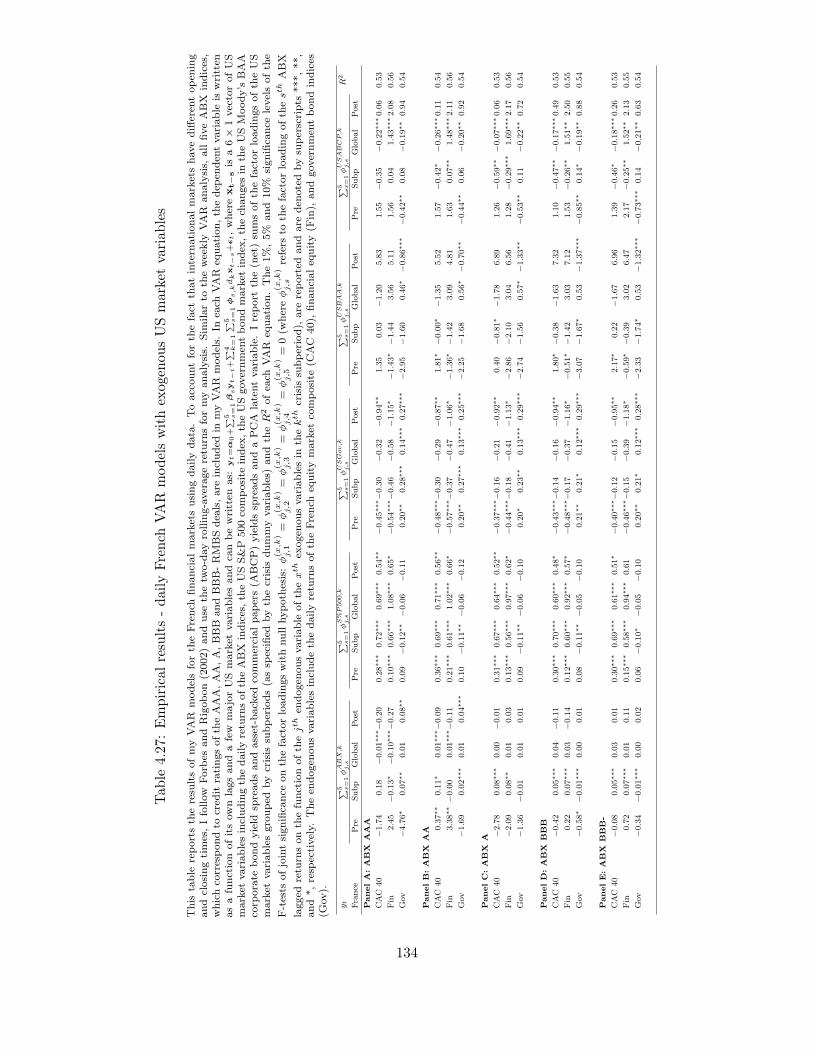
Tab
le4.27
:Empiricalresults-dailyFrench
VAR
modelswithexogenousUSmarket
variables
This
table
reportsth
eresu
ltsofmyVAR
modelsforth
eFrench
financialmarketsusingdailydata.Toaccountforth
efact
thatintern
ationalmarketshavedifferen
topen
ing
andclosingtimes,Ifollow
Forb
esandRigobon(2002)anduse
thetw
o-dayrolling-averageretu
rnsformyanalysis.
Sim
ilarto
theweekly
VAR
analysis,
allfiveABX
indices,
whichco
rrespondto
cred
itratingsofth
eAAA,AA,A,BBB
andBBB-RMBSdea
ls,are
included
inmyVAR
models.
Inea
chVAR
equation,th
edep
enden
tvariable
iswritten
asafunctionofitsownlagsandafew
majorUSmarket
variablesandca
nbewritten
as:
yt=α
0+∑ 5 s
=1βsyt−
i+∑ 4 k
=1
∑ 5 s=
1ϕ
s,k
dkxt−
s+ϵt,wherext−sis
a6×
1vectorofUS
market
variablesincludingth
edailyretu
rnsofth
eABX
indices,th
eUSS&P
500co
mposite
index
,th
eUSgovernmen
tbondmarket
index
,th
ech
anges
inth
eUSMoody’s
BAA
corp
orate
bondyield
spreadsandasset-backed
commercialpapers(A
BCP)yieldssp
readsandaPCA
latentvariable.Ireport
the(n
et)su
msofth
efactorloadingsofth
eUS
market
variablesgrouped
bycrisis
subperiods(assp
ecified
byth
ecrisis
dummyvariables)
andth
eR
2ofea
chVAR
equation.The1%,5%
and10%
significa
nce
levelsofth
e
F-tests
ofjointsignifica
nce
onth
efactorloadingswithnullhypoth
esis:ϕ(x
,k)
j,1
=ϕ(x
,k)
j,2
=ϕ(x
,k)
j,3
=ϕ(x
,k)
j,4
=ϕ(x
,k)
j,5
=0(w
hereϕ(x
,k)
j,s
refers
toth
efactorloadingofth
est
hABX
lagged
retu
rnsonth
efunctionofth
ejt
hen
dogen
ousvariable
ofth
exth
exogen
ousvariablesin
thekth
crisis
subperiod),
are
reported
andare
den
otedbysu
perscripts
***,**,
and*,resp
ectively.
Theen
dogen
ousvariablesincludeth
edailyretu
rnsofth
eFrench
equitymarket
composite
(CAC
40),
financialeq
uity(F
in),
andgovernmen
tbondindices
(Gov).
yt
∑ 5 s=1ϕABX
,kj,s
∑ 5 s=1ϕS%P500,k
j,s
∑ 5 s=1ϕUSGov,k
j,s
∑ 5 s=1ϕUSBAA,k
j,s
∑ 5 s=1ϕUSABCP,k
j,s
R2
France
Pre
Subp
Global
Post
Pre
Subp
Global
Post
Pre
Subp
Global
Post
Pre
Subp
Global
Post
Pre
Subp
Global
Post
PanelA:ABX
AAA
CAC
40
−1.74
0.18
−0.01∗∗
∗−0.20
0.28∗∗
∗0.72∗∗
∗0.69∗∗
∗0.54∗∗
−0.45∗∗
∗−0.30
−0.32
−0.94∗∗
1.35
0.03
−1.20
5.83
1.55
−0.35
−0.22∗∗
∗0.06
0.53
Fin
2.45
−0.13∗
−0.10∗∗
∗−0.27
0.10∗∗
∗0.66∗∗
∗1.08∗∗
∗0.65∗
−0.54∗∗
∗−0.46
−0.58
−1.15∗
−1.43∗
−1.44
3.56
5.11
1.56
0.04
1.43∗∗
∗2.08
0.56
Gov
−4.76∗
0.07∗∗
0.01
0.08∗∗
0.09
−0.12∗∗
−0.06
−0.11
0.20∗∗
0.28∗∗
∗0.14∗∗
∗0.27∗∗
∗−2.95
−1.60
0.46∗
−0.86∗∗
∗−0.42∗∗
0.08
−0.19∗∗
0.94
0.54
PanelB:ABX
AA
CAC
40
0.37∗∗
0.11∗
0.01∗∗
∗−0.09
0.36∗∗
∗0.69∗∗
∗0.71∗∗
∗0.56∗∗
−0.48∗∗
∗−0.30
−0.29
−0.87∗∗
1.81∗
−0.00∗
−1.35
5.52
1.57
−0.42∗
−0.26∗∗
∗0.11
0.54
Fin
3.38∗∗
−0.00
0.01∗∗
∗−0.11
0.21∗∗
∗0.61∗∗
∗1.02∗∗
∗0.66∗
−0.57∗∗
∗−0.37
−0.47
−1.06∗
−1.36∗
−1.42
3.09
4.81
1.63
0.07∗∗
1.48∗∗
∗2.11
0.56
Gov
−1.69
0.02∗∗
∗0.01
0.04∗∗
∗0.10
−0.11∗∗
−0.06
−0.12
0.20∗∗
0.27∗∗
∗0.13∗∗
∗0.25∗∗
∗−2.25
−1.68
0.56∗
−0.70∗∗
−0.44∗∗
0.06
−0.20∗∗
0.92
0.54
PanelC:ABX
A
CAC
40
−2.78
0.08∗∗
∗0.00
−0.01
0.31∗∗
∗0.67∗∗
∗0.64∗∗
∗0.52∗∗
−0.37∗∗
∗−0.16
−0.21
−0.92∗∗
0.40
−0.81∗
−1.78
6.89
1.26
−0.59∗∗
−0.07∗∗
∗0.06
0.53
Fin
−2.09
0.08∗∗
0.01
0.03
0.13∗∗
∗0.56∗∗
∗0.97∗∗
∗0.62∗
−0.44∗∗
∗−0.18
−0.41
−1.13∗
−2.86
−2.10
3.04
6.56
1.28
−0.29∗∗
∗1.69∗∗
∗2.17
0.56
Gov
−1.36
−0.01
0.01
0.01
0.09
−0.11∗∗
−0.06
−0.10
0.20∗
0.23∗∗
0.13∗∗
∗0.29∗∗
∗−2.74
−1.56
0.57∗
−1.33∗∗
−0.53∗∗
0.11
−0.22∗∗
0.72
0.54
PanelD:ABX
BBB
CAC
40
−0.42
0.05∗∗
∗0.04
−0.11
0.30∗∗
∗0.70∗∗
∗0.60∗∗
∗0.48∗
−0.43∗∗
∗−0.14
−0.16
−0.94∗∗
1.80∗
−0.38
−1.63
7.32
1.10
−0.47∗∗
−0.17∗∗
∗0.49
0.53
Fin
0.22
0.07∗∗
∗0.03
−0.14
0.12∗∗
∗0.60∗∗
∗0.92∗∗
∗0.57∗
−0.48∗∗
∗−0.17
−0.37
−1.16∗
−0.51∗
−1.42
3.03
7.12
1.53
−0.26∗∗
1.51∗∗
2.50
0.55
Gov
−0.58∗
−0.01∗∗
∗0.00
0.01
0.08
−0.11∗∗
−0.05
−0.10
0.21∗∗
0.21∗
0.12∗∗
∗0.29∗∗
∗−3.07
−1.67∗
0.53
−1.37∗∗
∗−0.85∗∗
0.14∗
−0.19∗∗
0.88
0.54
PanelE:ABX
BBB-
CAC
40
−0.08
0.05∗∗
∗0.03
0.01
0.30∗∗
∗0.69∗∗
∗0.61∗∗
∗0.51∗
−0.40∗∗
∗−0.12
−0.15
−0.95∗∗
2.17∗
0.22
−1.67
6.96
1.39
−0.46∗
−0.18∗∗
∗0.26
0.53
Fin
0.72
0.07∗∗
∗0.01
0.11
0.15∗∗
∗0.58∗∗
∗0.94∗∗
∗0.61
−0.46∗∗
∗−0.15
−0.39
−1.18∗
−0.59∗
−0.39
3.02
6.47
2.17
−0.25∗∗
1.52∗∗
2.13
0.55
Gov
−0.34
−0.01∗∗
∗0.00
0.02
0.06
−0.10∗
−0.05
−0.10
0.20∗∗
0.21∗
0.12∗∗
∗0.28∗∗
∗−2.33
−1.74∗
0.53
−1.32∗∗
∗−0.73∗∗
∗0.14
−0.21∗∗
0.63
0.54
134
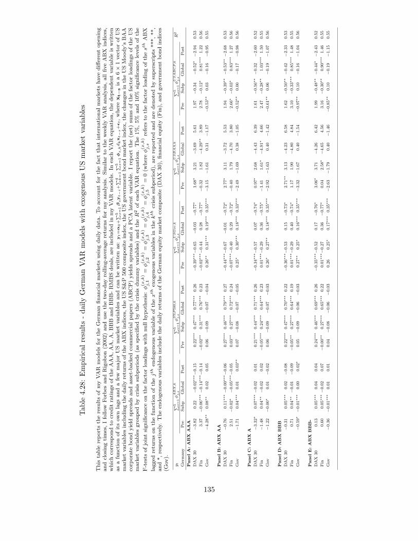
Tab
le4.28
:Empiricalresults-dailyGermanVAR
modelswithexogenousUSmarket
variables
This
table
reportsth
eresu
ltsofmyVAR
modelsforth
eGermanfinancialmarketsusingdailydata.Toaccountforth
efact
thatintern
ationalmarketshavedifferen
topen
ing
andclosingtimes,Ifollow
Forb
esandRigobon(2002)anduse
thetw
o-dayrolling-averageretu
rnsformyanalysis.
Sim
ilarto
theweekly
VAR
analysis,
allfiveABX
indices,
whichco
rrespondto
cred
itratingsofth
eAAA,AA,A,BBB
andBBB-RMBSdea
ls,are
included
inmyVAR
models.
Inea
chVAR
equation,th
edep
enden
tvariable
iswritten
asafunctionofitsownlagsandafew
majorUSmarket
variablesandca
nbewritten
as:
yt=α
0+∑ 5 s
=1βsyt−
i+∑ 4 k
=1
∑ 5 s=
1ϕ
s,k
dkxt−
s+ϵt,wherext−sis
a6×
1vectorofUS
market
variablesincludingth
edailyretu
rnsofth
eABX
indices,th
eUSS&P
500co
mposite
index
,th
eUSgovernmen
tbondmarket
index
,th
ech
anges
inth
eUSMoody’s
BAA
corp
orate
bondyield
spreadsandasset-backed
commercialpapers(A
BCP)yieldssp
readsandaPCA
latentvariable.Ireport
the(n
et)su
msofth
efactorloadingsofth
eUS
market
variablesgrouped
bycrisis
subperiods(assp
ecified
byth
ecrisis
dummyvariables)
andth
eR
2ofea
chVAR
equation.The1%,5%
and10%
significa
nce
levelsofth
e
F-tests
ofjointsignifica
nce
onth
efactorloadingswithnullhypoth
esis:ϕ(x
,k)
j,1
=ϕ(x
,k)
j,2
=ϕ(x
,k)
j,3
=ϕ(x
,k)
j,4
=ϕ(x
,k)
j,5
=0(w
hereϕ(x
,k)
j,s
refers
toth
efactorloadingofth
est
hABX
lagged
retu
rnsonth
efunctionofth
ejt
hen
dogen
ousvariable
ofth
exth
exogen
ousvariablesin
thekth
crisis
subperiod),
are
reported
andare
den
otedbysu
perscripts
***,**,
and*,resp
ectively.
Theen
dogen
ousvariablesincludeth
edailyretu
rnsofth
eGermaneq
uitymarket
composite
(DAX
30),
financialeq
uity(F
in),
andgovernmen
tbondindices
(Gov).
yt
∑ 5 s=1ϕABX
,kj,s
∑ 5 s=1ϕS%
P500,k
j,s
∑ 5 s=1ϕUSGov,k
j,s
∑ 5 s=1ϕUSBAA,k
j,s
∑ 5 s=1ϕUSABCP,k
j,s
R2
Germany
Pre
Subp
Global
Post
Pre
Subp
Global
Post
Pre
Subp
Global
Post
Pre
Subp
Global
Post
Pre
Subp
Global
Post
PanelA:ABX
AAA
DAX
30
−3.82
0.22
−0.02∗∗
∗−0.15
0.22∗∗
∗0.47∗∗
∗0.77∗∗
∗0.26
−0.39∗∗
∗−0.65
−0.03
−0.77∗
1.68∗
3.21
−3.69
5.61
1.97
−0.34
−0.52∗
−2.94
0.53
Fin
3.37
−0.06∗∗
∗−0.14∗∗
∗−0.14
−0.02∗∗
0.31∗∗
∗0.76∗∗
∗0.23
−0.02∗∗
∗−0.44
0.28
−0.77∗
−0.32
1.82
−4.29∗∗
3.89
2.78
−0.12∗
0.81∗∗
∗1.22
0.56
Gov
−4.28∗∗
0.08∗∗
0.02
0.05
0.06
−0.09
−0.07
−0.04
0.26∗∗
0.31∗∗
∗0.19∗∗
∗0.35∗∗
∗−3.15
−1.61
0.31
−1.17
−0.53∗∗
0.03
−0.16
−0.95
0.55
PanelB:ABX
AA
DAX
30
−0.76
0.11∗∗
∗−0.00∗∗
∗−0.06
0.27∗∗
∗0.46∗∗
∗0.79∗∗
∗0.27
−0.44∗∗
∗−0.67
−0.01
−0.72∗
2.77∗
3.11
−3.72
5.53
1.94
−0.39∗∗
−0.53∗∗
−2.68
0.53
Fin
2.51
−0.02∗
−0.05∗∗
∗−0.05
0.03∗∗
0.27∗∗
∗0.72∗∗
∗0.24
−0.07∗∗
∗−0.40
0.29
−0.72∗
−0.40
1.79
−4.70
3.80
2.66∗
−0.03∗
0.83∗∗
∗1.27
0.56
Gov
−1.71
0.04∗∗
∗0.01
0.03∗∗
0.07
−0.08
−0.07
−0.05
0.25∗
0.30∗∗
∗0.18∗∗
∗0.33∗∗
∗−2.49
−1.69
0.38
−1.05
−0.52∗∗
0.00
−0.17
−0.98
0.56
PanelC:ABX
A
DAX
30
−3.32∗
0.07∗∗
∗−0.02
0.01
0.21∗∗
∗0.44∗∗
∗0.71∗∗
∗0.26
−0.34∗∗
∗−0.57
0.07
−0.74∗
0.97∗
2.68
−4.43
6.39
1.61
−0.56∗∗
−0.32
−2.60
0.52
Fin
−1.48
0.04∗∗
−0.02
0.02
−0.05∗∗
∗0.24∗∗
∗0.64∗∗
∗0.23
0.01∗∗
∗−0.29
0.36
−0.75∗
−1.41
1.61∗
−4.91∗
4.66
2.47
−0.28∗∗
1.03∗∗
∗1.50
0.55
Gov
−1.22
−0.00∗
0.01
−0.02
0.06
−0.09
−0.07
−0.03
0.26∗
0.27∗∗
0.18∗∗
∗0.35∗∗
∗−2.92
−1.63
0.40
−1.42
−0.61∗∗
0.06
−0.19
−1.07
0.56
PanelD:ABX
BBB
DAX
30
−0.31
0.05∗∗
∗0.02
−0.08
0.22∗∗
∗0.47∗∗
∗0.70∗∗
∗0.22
−0.36∗∗
∗−0.53
0.15
−0.73∗
2.71∗∗
3.13
−4.23
6.58
1.62
−0.50∗∗
−0.42
−2.33
0.53
Fin
0.71
0.04∗∗
−0.01
−0.09
−0.05∗∗
0.27∗∗
∗0.64∗∗
∗0.19
0.01∗∗
∗−0.29
0.40
−0.74∗
1.17
1.90
−4.80
4.84
3.10
−0.33∗∗
∗0.85∗∗
∗1.48
0.55
Gov
−0.59∗
−0.01∗∗
∗0.00
0.02∗
0.05
−0.09
−0.06
−0.03
0.27∗∗
0.25∗
0.16∗∗
∗0.35∗∗
∗−3.32
−1.67
0.40
−1.54
−0.97∗∗
0.10
−0.16
−1.04
0.56
PanelE:ABX
BBB-
DAX
30
0.13
0.05∗∗
∗0.04
0.04
0.24∗∗
∗0.46∗∗
∗0.69∗∗
∗0.26
−0.35∗∗
∗−0.52
0.17
−0.76∗
3.06∗
3.71
−4.26
6.42
1.99
−0.48∗∗
−0.44∗
−2.43
0.52
Fin
0.60
0.05∗∗
∗−0.02
0.07
−0.00∗∗
0.27∗∗
∗0.65∗∗
∗0.22
0.01∗∗
∗−0.27
0.36
−0.77∗
0.04
2.58∗
−4.65
4.56
3.16
−0.30∗∗
0.90∗∗
∗1.46
0.55
Gov
−0.36
−0.01∗∗
∗0.01
0.01
0.04
−0.08
−0.06
−0.03
0.26
0.25∗
0.17∗∗
∗0.35∗∗
∗−2.63
−1.79
0.40
−1.46
−0.85∗∗
0.10
−0.19
−1.15
0.55
135

Tab
le4.29
:Empiricalresults-dailyJapaneseVAR
modelswithexogenousUSmarket
variables
This
table
reportsth
eresu
ltsofmyVAR
modelsforth
eJapanesefinancialmarketsusingdailydata.Toaccountforth
efact
thatintern
ationalmarketshavedifferen
topen
ing
andclosingtimes,Ifollow
Forb
esandRigobon(2002)anduse
thetw
o-dayrolling-averageretu
rnsformyanalysis.
Sim
ilarto
theweekly
VAR
analysis,
allfiveABX
indices,
whichco
rrespondto
cred
itratingsofth
eAAA,AA,A,BBB
andBBB-RMBSdea
ls,are
included
inmyVAR
models.
Inea
chVAR
equation,th
edep
enden
tvariable
iswritten
asafunctionofitsownlagsandafew
majorUSmarket
variablesandca
nbewritten
as:
yt=α
0+∑ 5 s
=1βsyt−
i+∑ 4 k
=1
∑ 5 s=
1ϕ
s,k
dkxt−
s+ϵt,wherext−sis
a6×
1vectorofUS
market
variablesincludingth
edailyretu
rnsofth
eABX
indices,th
eUSS&P
500co
mposite
index
,th
eUSgovernmen
tbondmarket
index
,th
ech
anges
inth
eUSMoody’s
BAA
corp
orate
bondyield
spreadsandasset-backed
commercialpapers(A
BCP)yieldssp
readsandaPCA
latentvariable.Ireport
the(n
et)su
msofth
efactorloadingsofth
eUS
market
variablesgrouped
bycrisis
subperiods(assp
ecified
byth
ecrisis
dummyvariables)
andth
eR
2ofea
chVAR
equation.The1%,5%
and10%
significa
nce
levelsofth
e
F-tests
ofjointsignifica
nce
onth
efactorloadingswithnullhypoth
esis:ϕ(x
,k)
j,1
=ϕ(x
,k)
j,2
=ϕ(x
,k)
j,3
=ϕ(x
,k)
j,4
=ϕ(x
,k)
j,5
=0(w
hereϕ(x
,k)
j,s
refers
toth
efactorloadingofth
est
hABX
lagged
retu
rnson
thefunction
ofth
ejt
hen
dogen
ousvariable
ofth
exth
exogen
ousvariablesin
thekth
crisis
subperiod),
are
reported
and
are
den
oted
bysu
perscripts
***,
**,and*,resp
ectively.
Theen
dogen
ousvariablesincludeth
edailyretu
rnsofth
eJapaneseeq
uitymarket
composite
(Nikkei
225),
financialeq
uity(F
in),
andgovernmen
tbond
indices
(Gov).
yt
∑ 5 s=1ϕABX
,kj,s
∑ 5 s=1ϕS%
P500,k
j,s
∑ 5 s=1ϕUSGov,k
j,s
∑ 5 s=1ϕUSBAA,k
j,s
∑ 5 s=1ϕUSABCP,k
j,s
R2
Japan
Pre
Subp
Global
Post
Pre
Subp
Global
Post
Pre
Subp
Global
Post
Pre
Subp
Global
Post
Pre
Subp
Global
Post
PanelA:ABX
AAA
Nikkei
225
−10.56∗
−0.24
−0.21∗∗
0.04
0.27
0.88∗∗
∗0.97∗∗
∗0.33∗∗
∗−0.56
−0.08
−0.53
−0.49∗∗
∗21.84∗∗
−2.41∗∗
−1.40
−1.00
0.21
−0.31∗∗
−0.11
−3.85
0.64
Fin
−8.30∗∗
−0.35∗∗
∗−0.10
0.02
0.02
0.92∗∗
∗0.83∗∗
∗0.26
−0.20
0.59
−0.54
−0.43∗
23.14
−2.55
1.03
−3.14
−0.17
−0.41
0.62
−4.61
0.62
Gov
2.34∗∗
0.00∗∗
∗−0.00∗
−0.01
0.12
−0.05
0.01∗∗
−0.00
0.21∗∗
∗0.15∗∗
∗0.15∗∗
∗0.17∗∗
∗−0.01∗∗
−0.09
−0.27
0.27
−0.22∗∗
0.05∗∗
0.01∗∗
∗0.32
0.56
PanelB:ABX
AA
Nikkei
225
1.95∗
−0.03
−0.10
−0.01
0.16∗∗
0.86∗∗
∗0.97∗∗
∗0.34∗∗
∗−0.48
−0.09
−0.54
−0.47∗∗
∗24.76∗∗
∗−1.67∗∗
−1.76
−1.35
0.13
−0.42∗
−0.05
−3.79
0.64
Fin
6.97
−0.10∗∗
−0.05
−0.01
−0.12
0.87∗∗
∗0.84∗∗
∗0.27
−0.08
0.59
−0.51
−0.40∗
26.28
−1.76
0.91
−3.48
0.03
−0.44
0.66
−4.70
0.62
Gov
−0.70∗
0.01∗∗
∗0.00
0.00
0.12
−0.05
0.00∗∗
−0.00
0.21∗∗
∗0.15∗∗
∗0.15∗∗
∗0.17∗∗
∗−0.61∗
−0.03
−0.27
0.28
−0.25
0.05
0.00∗∗
∗0.30
0.56
PanelC:ABX
A
Nikkei
225
0.96∗∗
∗0.01
−0.05
0.02
0.13∗∗
0.87∗∗
∗0.92∗∗
∗0.32∗∗
∗−0.45
−0.01
−0.49
−0.46∗∗
∗24.12∗∗
∗−1.80∗∗
−1.45
−1.25
0.38
−0.49∗∗
0.01
−3.82
0.64
Fin
4.31∗∗
−0.00
−0.02
0.01
−0.16
0.88∗∗
∗0.83∗∗
∗0.27
−0.11
0.67
−0.47
−0.43∗
26.78∗
−1.83
0.81
−3.24
0.56
−0.59
0.61
−4.49
0.62
Gov
0.05∗
−0.01∗∗
∗−0.00
−0.01
0.12
−0.05
0.01∗∗
−0.00
0.22∗∗
∗0.13∗∗
∗0.14∗∗
∗0.17∗∗
∗−0.56∗∗
0.03
−0.26
0.29
−0.22∗
0.08
0.01∗∗
∗0.29
0.56
PanelD:ABX
BBB
Nikkei
225
0.73
−0.00∗
−0.02
−0.09
0.17∗
0.87∗∗
∗0.92∗∗
∗0.31∗∗
∗−0.54
−0.04
−0.49
−0.46∗∗
∗25.88∗∗
∗−1.57∗
−0.99
−0.90
0.80
−0.47∗
−0.09
−3.53
0.64
Fin
2.03∗
−0.02
0.02∗∗
0.02
−0.05
0.86∗∗
∗0.77∗∗
∗0.26
−0.21
0.58
−0.42
−0.42∗
28.63∗
−1.59
1.16
−3.33
1.51
−0.54
0.65
−4.61
0.63
Gov
−0.18∗∗
−0.00∗∗
−0.00
0.01
0.12
−0.05
0.00∗
−0.00
0.22∗∗
∗0.14∗∗
∗0.14∗∗
∗0.17∗∗
∗−0.87
−0.06
−0.26
0.25
−0.40∗∗
0.07
0.02∗∗
0.26
0.56
PanelE:ABX
BBB-
Nikkei
225
0.99
−0.01
−0.02
−0.08
0.18∗
0.89∗∗
∗0.93∗∗
∗0.33∗∗
∗−0.56
−0.08
−0.48
−0.47∗∗
∗25.82∗∗
∗−1.52∗∗
−0.86
−1.15
1.25
−0.50∗∗
0.03
−3.52
0.64
Fin
1.51
−0.04
0.00
−0.03
−0.04
0.89∗∗
∗0.80∗∗
∗0.26
−0.22
0.55
−0.42
−0.44∗
26.97∗
−1.88
1.09
−3.30
1.53
−0.59
0.75
−4.61
0.62
Gov
−0.17∗∗
∗0.00∗∗
0.00
0.01
0.13
−0.05
0.00∗∗
−0.00
0.22∗∗
∗0.14∗∗
∗0.15∗∗
∗0.17∗∗
∗−0.68
−0.01
−0.24
0.27
−0.44∗∗
0.07
0.01∗∗
∗0.27
0.56
136

Tab
le4.30
:Subprimean
dglob
alcrises
-conditionalandunconditionalcorrelationcoeffi
cients
ontheinternationalequitymarkets
This
table
reportsth
eco
nditionalco
rrelation
coeffi
cien
ts,standard
dev
iations,
unco
nditional(adjusted
forheterosked
asticityfollowingForb
esand
Rigobon
(2002)assh
own
in
Equation4.8)co
rrelationco
efficien
tsbetweenea
chG5intern
ationalbroadeq
uitymarket
andth
eUSstru
cturedfinance
market
(mea
suredbyth
eABX
indices)ofth
efullsample
and
thecrisis
subperiods.
All
theco
rrelation
coeffi
cien
tshavebeen
transform
edusingFisher
transform
ation
assh
own
inEquation
4.13and
thestandard
dev
iations(ofth
e
ABX
indices)havebeentransform
edusingEquation4.14.Rep
orted
are
thestatisticsofth
etw
o-sample
t-tests(one-sided
tests,
assh
ownin
Equation4.15)ofth
eco
nditional
andunco
nditionalco
rrelationco
efficien
tsbetweenth
efullsample
andth
ecrisis
subperiods,
resp
ectively.
The‘Y
’in
theco
lumnswithhea
der
‘Contagion’report
thepresence
of
contagionwhen
thetest
statisticsare
larger
thanth
ecriticalvalues
and‘N
’oth
erwise(forth
eabsence
ofco
ntagion).
ρadj,ρcon
andσ
referto
the(h
eterosked
asticity-adjusted
)
unco
nditionalco
rrelationco
efficien
ts,co
nditionalco
rrelationco
efficien
tsandth
estandard
dev
iationsofth
eintern
ationalmarkets,
resp
ectively.
Broad
equity
markets
Pre-crisis
Subprim
eGlobal
Post-crisis
Full
Full
vsSubprim
e(C
)Full
vsGlobal(C
)Full
vsSubprim
e(A
dj.)
Full
vsGlobal(A
dj.)
Country
ABX
ρadj
ρcon
σρadj
ρcon
σρadj
ρcon
σρadj
ρcon
σρadj
σuncon
t-stat
Contagion
t-stat
Contagion
t-stat
Contagion
t-stat
Contagion
US
AAA
-0.99
-0.09
0.32
0.64
0.41
0.51
0.22
0.35
1.30
0.52
0.40
0.65
0.35
0.81
1.12
N0.08
N5.87
Y-2.14
N
AA
-0.99
-0.13
0.32
0.57
0.36
0.51
0.27
0.40
1.30
0.44
0.40
0.65
0.37
0.81
-0.08
N0.54
N3.81
Y-1.68
N
A-0.95
-0.04
0.32
0.48
0.48
0.51
0.19
0.29
1.32
0.09
0.07
0.66
0.22
0.81
4.34
Y1.20
N4.28
Y-0.55
N
BBB
0.98
0.20
0.32
0.39
0.43
0.49
0.10
0.14
1.30
-0.07
-0.06
0.66
0.12
0.81
5.08
Y0.43
N4.26
Y-0.22
N
BBB-
0.98
0.28
0.33
0.37
0.42
0.50
0.15
0.21
1.31
0.03
0.02
0.65
0.16
0.81
4.23
Y0.84
N3.32
Y-0.16
N
UK
AAA
-0.50
-0.01
0.40
0.52
0.31
0.54
0.19
0.30
1.06
0.55
0.43
0.63
0.33
0.74
-0.30
N-0.51
N3.41
Y-2.37
N
AA
0.63
0.01
0.41
0.56
0.36
0.54
0.23
0.33
1.07
0.46
0.41
0.63
0.35
0.74
0.16
N-0.33
N3.95
Y-2.04
N
A1.00
0.17
0.40
0.36
0.36
0.53
0.18
0.28
1.08
0.09
0.07
0.63
0.22
0.74
2.31
Y1.11
N2.34
Y-0.54
N
BBB
0.99
0.34
0.40
0.30
0.34
0.52
0.09
0.12
1.07
-0.03
-0.02
0.63
0.13
0.74
3.36
Y-0.13
N2.67
Y-0.65
N
BBB-
0.99
0.36
0.40
0.24
0.29
0.52
0.12
0.17
1.08
0.06
0.05
0.63
0.16
0.74
1.98
Y0.23
N1.32
N-0.56
N
France
AAA
-0.66
-0.01
0.43
0.47
0.27
0.48
0.21
0.33
1.06
0.57
0.44
0.74
0.34
0.78
-1.15
N-0.23
N2.29
Y-2.31
N
AA
0.94
0.04
0.43
0.53
0.33
0.48
0.23
0.34
1.06
0.47
0.42
0.74
0.36
0.78
-0.45
N-0.31
N3.24
Y-2.17
N
A0.99
0.12
0.43
0.32
0.32
0.47
0.19
0.29
1.07
0.11
0.09
0.74
0.21
0.78
1.69
Y1.40
N1.78
Y-0.37
N
BBB
0.99
0.33
0.43
0.27
0.31
0.47
0.10
0.14
1.06
-0.06
-0.04
0.74
0.11
0.78
2.97
Y0.45
N2.37
Y-0.19
N
BBB-
0.99
0.35
0.43
0.24
0.27
0.47
0.13
0.19
1.07
0.10
0.07
0.74
0.16
0.78
1.81
Y0.51
N1.20
N-0.38
N
Germany
AAA
-0.19
0.00
0.42
0.46
0.26
0.46
0.19
0.31
1.06
0.55
0.43
0.70
0.32
0.75
-0.94
N-0.17
N2.46
Y-2.16
N
AA
-0.46
-0.01
0.42
0.50
0.30
0.46
0.22
0.33
1.06
0.44
0.40
0.70
0.33
0.75
-0.47
N-0.08
N2.96
Y-1.90
N
A0.99
0.10
0.42
0.36
0.36
0.45
0.16
0.24
1.08
0.14
0.11
0.70
0.19
0.76
2.68
Y0.99
N2.77
Y-0.48
N
BBB
0.99
0.31
0.42
0.32
0.36
0.45
0.11
0.16
1.07
-0.03
-0.02
0.70
0.12
0.76
3.76
Y0.60
N3.01
Y-0.13
N
BBB-
0.99
0.36
0.42
0.32
0.37
0.45
0.14
0.20
1.08
0.06
0.04
0.70
0.15
0.76
3.44
Y0.81
N2.61
Y-0.13
N
Japan
AAA
0.87
0.02
0.58
0.15
0.08
0.60
0.18
0.29
1.23
0.28
0.20
0.62
0.22
0.81
-2.12
N1.24
N-1.10
N-0.66
N
AA
1.00
0.26
0.60
0.11
0.06
0.60
0.18
0.27
1.22
0.21
0.18
0.61
0.21
0.80
-2.21
N1.07
N-1.46
N-0.48
N
A1.00
0.15
0.59
0.04
0.04
0.59
0.15
0.24
1.23
0.13
0.10
0.62
0.17
0.81
-1.96
N1.10
N-1.94
N-0.33
N
BBB
0.96
0.14
0.58
0.04
0.04
0.58
0.04
0.06
1.23
-0.05
-0.04
0.62
0.06
0.81
-0.22
N-0.02
N-0.30
N-0.28
N
BBB-
0.94
0.16
0.58
0.04
0.05
0.59
0.11
0.15
1.24
-0.03
-0.02
0.62
0.10
0.81
-0.84
N0.75
N-0.93
N0.04
N
137
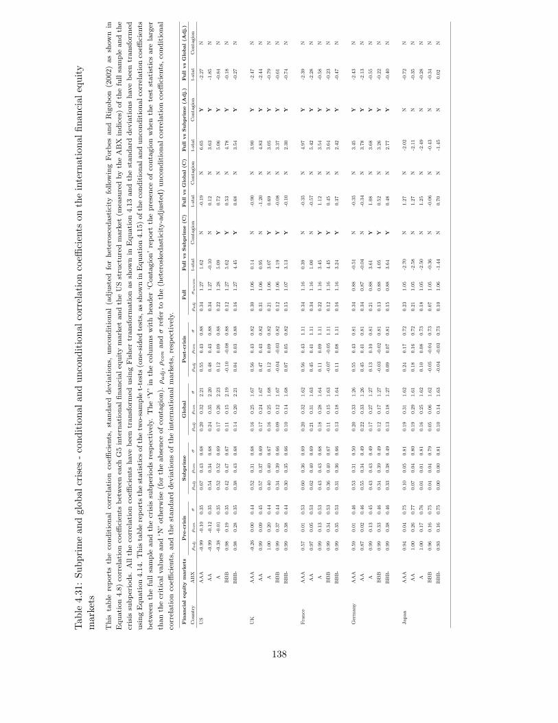
Tab
le4.31:Subprimean
dglob
alcrises
-conditionalandunconditionalcorrelationcoeffi
cients
ontheinternationalfinan
cial
equity
markets
This
table
reportsth
eco
nditionalco
rrelation
coeffi
cien
ts,standard
dev
iations,
unco
nditional(adjusted
forheterosced
asticity
followingForb
esand
Rigobon
(2002)assh
own
in
Equation4.8)co
rrelationco
efficien
tsbetweenea
chG5intern
ationalfinancialeq
uitymarket
andth
eUSstru
cturedmarket
(mea
suredbyth
eABX
indices)ofth
efullsample
andth
e
crisis
subperiods.
Allth
eco
rrelationco
efficien
tshavebeentransform
edusingFisher
transform
ationassh
ownin
Equation4.13andth
estandard
dev
iationshavebeentransform
ed
usingEquation4.14.Thistable
reportsth
estatisticsofth
etw
o-sample
t-tests(one-sided
tests,
assh
ownin
Equation4.15)ofth
eco
nditionalandunco
nditionalco
rrelationco
efficien
ts
betweenth
efullsample
andth
ecrisis
subperiodsresp
ectively.
The‘Y
’in
theco
lumnswithhea
der
‘Contagion’report
thepresence
ofco
ntagionwhen
thetest
statisticsare
larger
thanth
ecriticalvalues
and‘N
’oth
erwise(forth
eabsence
ofco
ntagion).
ρadj,ρconandσreferto
the(h
eterosked
asticity-adjusted
)unco
nditionalco
rrelationco
efficien
ts,co
nditional
correlationco
efficien
ts,andth
estandard
dev
iationsofth
eintern
ationalmarkets,
resp
ectively.
Fin
ancialequity
markets
Pre-crisis
Subprim
eGlobal
Post-crisis
Full
Full
vsSubprim
e(C
)Full
vsGlobal(C
)Full
vsSubprim
e(A
dj.)
Full
vsGlobal(A
dj.)
Country
ABX
ρadj
ρcon
σρadj
ρcon
σρadj
ρcon
σρadj
ρcon
σρadj
σuncon
t-stat
Contagion
t-stat
Contagion
t-stat
Contagion
t-stat
Contagion
US
AAA
-0.99
-0.10
0.35
0.67
0.43
0.68
0.20
0.32
2.21
0.55
0.43
0.88
0.34
1.27
1.62
N-0.19
N6.65
Y-2.27
N
AA
-0.99
-0.12
0.35
0.54
0.34
0.68
0.24
0.35
2.20
0.48
0.43
0.88
0.34
1.27
-0.10
N0.12
N3.63
Y-1.85
N
A-0.38
-0.01
0.35
0.52
0.52
0.69
0.17
0.26
2.23
0.12
0.09
0.88
0.22
1.28
5.09
Y0.72
N5.06
Y-0.84
N
BBB
0.98
0.19
0.35
0.42
0.47
0.67
0.11
0.15
2.19
-0.10
-0.08
0.88
0.12
1.27
5.62
Y0.53
N4.78
Y-0.18
N
BBB-
0.98
0.28
0.35
0.38
0.43
0.68
0.14
0.20
2.21
0.04
0.03
0.88
0.16
1.27
4.45
Y0.68
N3.54
Y-0.27
N
UK
AAA
-0.26
0.00
0.44
0.52
0.31
0.68
0.16
0.25
1.67
0.56
0.43
0.82
0.30
1.06
0.14
N-0.90
N3.90
Y-2.47
N
AA
0.99
0.09
0.45
0.57
0.37
0.69
0.17
0.24
1.67
0.47
0.43
0.82
0.31
1.06
0.95
N-1.20
N4.83
Y-2.44
N
A1.00
0.20
0.44
0.40
0.40
0.67
0.16
0.25
1.68
0.12
0.09
0.82
0.21
1.06
3.07
Y0.69
N3.05
Y-0.79
N
BBB
0.99
0.37
0.44
0.34
0.39
0.66
0.09
0.12
1.67
-0.04
-0.03
0.82
0.12
1.06
4.19
Y-0.08
N3.37
Y-0.61
N
BBB-
0.99
0.38
0.44
0.30
0.35
0.66
0.10
0.14
1.68
0.07
0.05
0.82
0.15
1.07
3.13
Y-0.10
N2.30
Y-0.74
N
France
AAA
0.57
0.01
0.53
0.60
0.36
0.69
0.20
0.32
1.62
0.56
0.43
1.11
0.34
1.16
0.39
N-0.35
N4.97
Y-2.39
N
AA
0.97
0.05
0.53
0.62
0.40
0.69
0.21
0.31
1.63
0.45
0.41
1.11
0.34
1.16
1.00
N-0.57
N5.42
Y-2.28
N
A0.99
0.13
0.53
0.43
0.43
0.68
0.18
0.28
1.64
0.11
0.09
1.11
0.22
1.16
3.45
Y1.12
N3.54
Y-0.58
N
BBB
0.99
0.34
0.53
0.36
0.40
0.67
0.11
0.15
1.63
-0.07
-0.05
1.11
0.12
1.16
4.45
Y0.45
N3.64
Y-0.23
N
BBB-
0.99
0.35
0.53
0.31
0.36
0.66
0.13
0.18
1.64
0.11
0.08
1.11
0.16
1.16
3.24
Y0.37
N2.42
Y-0.47
N
Germany
AAA
0.59
0.01
0.46
0.53
0.31
0.50
0.20
0.33
1.26
0.55
0.43
0.81
0.34
0.88
-0.51
N-0.35
N3.45
Y-2.43
N
AA
0.87
0.02
0.46
0.55
0.34
0.49
0.22
0.33
1.26
0.45
0.41
0.81
0.34
0.87
-0.04
N-0.34
N3.78
Y-2.13
N
A0.99
0.13
0.45
0.43
0.43
0.49
0.17
0.27
1.27
0.13
0.10
0.81
0.21
0.88
3.61
Y1.08
N3.68
Y-0.55
N
BBB
0.99
0.33
0.46
0.34
0.39
0.49
0.12
0.17
1.27
-0.03
-0.02
0.81
0.13
0.88
4.05
Y0.52
N3.26
Y-0.22
N
BBB-
0.99
0.38
0.46
0.33
0.38
0.49
0.13
0.18
1.27
0.09
0.07
0.81
0.15
0.88
3.64
Y0.48
N2.77
Y-0.40
N
Japan
AAA
0.94
0.04
0.75
0.10
0.05
0.81
0.19
0.31
1.62
0.24
0.17
0.72
0.23
1.05
-2.70
N1.27
N-2.02
N-0.72
N
AA
1.00
0.26
0.77
0.07
0.04
0.80
0.19
0.29
1.61
0.18
0.16
0.72
0.21
1.05
-2.58
N1.27
N-2.11
N-0.35
N
A1.00
0.17
0.76
0.01
0.01
0.81
0.16
0.25
1.62
0.10
0.08
0.73
0.18
1.05
-2.50
N1.25
N-2.49
N-0.28
N
BBB
0.96
0.16
0.75
0.04
0.04
0.79
0.05
0.06
1.62
-0.05
-0.04
0.73
0.07
1.05
-0.36
N-0.06
N-0.43
N-0.34
N
BBB-
0.93
0.16
0.75
0.00
0.00
0.81
0.10
0.14
1.63
-0.04
-0.03
0.73
0.10
1.06
-1.44
N0.70
N-1.45
N0.02
N
138
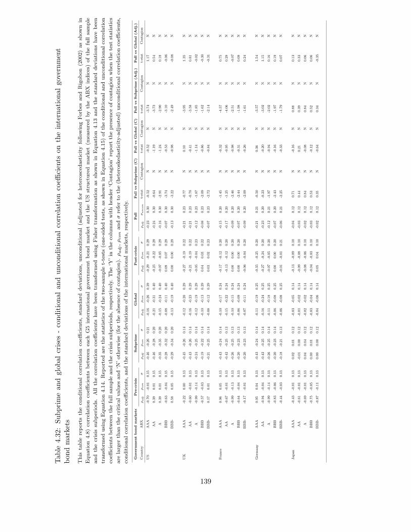
Tab
le4.32
:Subprimean
dglob
alcrises
-conditionalandunconditionalcorrelationcoeffi
cients
ontheinternationalgovernment
bon
dmarkets
This
table
reportsth
eco
nditionalco
rrelation
coeffi
cien
ts,standard
dev
iations,
unco
nditional(adjusted
forheterosced
asticity
followingForb
esand
Rigobon
(2002)assh
own
in
Equation
4.8)co
rrelation
coeffi
cien
tsbetween
each
G5intern
ationalgovernmen
tbond
market
and
theUS
stru
ctured
market
(mea
sured
byth
eABX
indices)ofth
efull
sample
and
thecrisis
subperiods.
All
theco
rrelation
coeffi
cien
tshavebeen
transform
edusingFisher
transform
ation
assh
own
inEquation
4.13and
thestandard
dev
iationshavebeen
transform
edusingEquation4.14.Rep
orted
are
thestatisticsofth
etw
o-sample
t-tests(one-sided
tests,
assh
ownin
Equation4.15)ofth
eco
nditionalandunco
nditionalco
rrelation
coeffi
cien
tsbetweenth
efullsample
andth
ecrisis
subperiods,
resp
ectively.
The‘Y
’in
theco
lumnswithhea
der
‘Contagion’report
thepresence
ofco
ntagionwhen
thetest
statistics
are
larger
thanth
ecriticalvalues
and‘N
’oth
erwise(forth
eabsence
ofco
ntagion).
ρadj,ρconandσreferto
the(h
eterosked
asticity-adjusted
)unco
nditionalco
rrelationco
efficien
ts,
conditionalco
rrelationco
efficien
ts,andth
estandard
dev
iationsofth
eintern
ationalmarkets,
resp
ectively.
Governm
entbond
markets
Pre-crisis
Subprim
eGlobal
Post-crisis
Full
Full
vsSubprim
e(C
)Full
vsGlobal(C
)Full
vsSubprim
e(A
dj.)
Full
vsGlobal(A
dj.)
Country
ABX
ρadj
ρcon
σρadj
ρcon
σρadj
ρcon
σρadj
ρcon
σρadj
σuncon
t-stat
Contagion
t-stat
Contagion
t-stat
Contagion
t-stat
Contagion
US
AAA
-0.70
-0.01
0.15
-0.46
-0.26
0.21
-0.16
-0.26
0.39
-0.29
-0.21
0.29
-0.23
0.30
-0.52
N-0.52
N-3.74
N1.17
N
AA
0.39
0.01
0.15
-0.46
-0.28
0.20
-0.21
-0.31
0.40
-0.25
-0.22
0.29
-0.24
0.30
-0.64
N-1.19
N-3.73
N0.54
N
A0.39
0.01
0.15
-0.35
-0.35
0.20
-0.15
-0.24
0.40
-0.07
-0.05
0.29
-0.16
0.30
-2.91
N-1.24
N-2.90
N0.18
N
BBB
-0.63
-0.04
0.15
-0.28
-0.32
0.20
-0.08
-0.11
0.40
0.09
0.07
0.29
-0.07
0.30
-3.74
N-0.53
N-3.10
N-0.06
N
BBB-
0.58
0.05
0.15
-0.29
-0.34
0.20
-0.13
-0.19
0.40
0.00
0.00
0.29
-0.13
0.30
-3.22
N-0.98
N-2.49
N-0.08
N
UK
AAA
-0.22
0.00
0.13
-0.45
-0.26
0.14
-0.12
-0.20
0.29
-0.27
-0.19
0.22
-0.21
0.23
-0.77
N0.10
N-3.95
N1.35
N
AA
-0.60
-0.01
0.13
-0.43
-0.26
0.14
-0.16
-0.23
0.29
-0.21
-0.19
0.22
-0.21
0.23
-0.78
N-0.41
N-3.58
N0.81
N
A-0.99
-0.14
0.13
-0.24
-0.25
0.14
-0.12
-0.19
0.29
-0.05
-0.04
0.23
-0.12
0.23
-1.87
N-1.14
N-1.85
N-0.02
N
BBB
-0.57
-0.03
0.13
-0.19
-0.22
0.14
-0.10
-0.13
0.29
0.04
0.03
0.22
-0.08
0.23
-2.09
N-0.86
N-1.62
N-0.30
N
BBB-
0.17
0.01
0.13
-0.21
-0.25
0.14
-0.08
-0.12
0.29
0.03
0.02
0.23
-0.07
0.23
-2.72
N-0.84
N-2.14
N-0.31
N
France
AAA
0.96
0.05
0.13
-0.43
-0.24
0.14
-0.10
-0.17
0.24
-0.17
-0.12
0.20
-0.15
0.20
-1.45
N-0.32
N-4.57
N0.75
N
AA
-0.67
-0.01
0.13
-0.42
-0.25
0.13
-0.15
-0.22
0.24
-0.13
-0.12
0.20
-0.17
0.20
-1.25
N-0.95
N-4.06
N0.29
N
A-0.99
-0.13
0.13
-0.26
-0.25
0.13
-0.10
-0.15
0.24
0.00
0.00
0.20
-0.09
0.20
-2.46
N-0.98
N-2.51
N-0.07
N
BBB
-0.64
-0.04
0.13
-0.20
-0.23
0.13
-0.06
-0.09
0.24
0.00
0.00
0.20
-0.07
0.20
-2.44
N-0.31
N-1.98
N0.09
N
BBB-
-0.17
-0.01
0.13
-0.20
-0.23
0.13
-0.07
-0.11
0.24
-0.06
-0.04
0.20
-0.09
0.20
-2.09
N-0.26
N-1.61
N0.24
N
Germany
AAA
0.95
0.04
0.13
-0.43
-0.24
0.14
-0.11
-0.19
0.25
-0.35
-0.25
0.20
-0.21
0.21
-0.50
N0.36
N-3.57
N1.54
N
AA
-0.94
-0.04
0.13
-0.42
-0.25
0.14
-0.16
-0.24
0.25
-0.27
-0.24
0.20
-0.23
0.20
-0.23
N-0.20
N-3.02
N1.15
N
A-0.99
-0.14
0.13
-0.26
-0.25
0.14
-0.11
-0.18
0.25
-0.07
-0.05
0.20
-0.12
0.21
-1.97
N-0.94
N-2.02
N0.16
N
BBB
-0.83
-0.06
0.13
-0.20
-0.23
0.14
-0.06
-0.08
0.25
0.00
0.00
0.20
-0.07
0.20
-2.43
N-0.16
N-1.97
N0.19
N
BBB-
-0.44
-0.03
0.13
-0.18
-0.21
0.13
-0.06
-0.08
0.25
-0.01
-0.01
0.21
-0.06
0.21
-2.25
N-0.33
N-1.79
N0.07
N
Japan
AAA
-0.43
-0.01
0.13
0.02
0.01
0.12
-0.03
-0.05
0.14
-0.13
-0.09
0.10
-0.04
0.12
0.71
N-0.16
N0.88
N0.13
N
AA
-0.61
-0.01
0.13
-0.01
0.00
0.12
-0.01
-0.02
0.14
-0.09
-0.08
0.10
-0.03
0.12
0.44
N0.21
N0.39
N0.33
N
A-0.69
-0.01
0.13
0.04
0.04
0.12
-0.02
-0.02
0.14
-0.08
-0.06
0.10
-0.02
0.12
0.84
N-0.08
N0.84
N0.06
N
BBB
-0.75
-0.05
0.13
0.00
0.01
0.12
-0.03
-0.04
0.14
-0.04
-0.03
0.10
-0.03
0.12
0.53
N-0.12
N0.52
N0.06
N
BBB-
-0.87
-0.11
0.13
0.00
0.00
0.12
-0.04
-0.06
0.14
0.05
0.04
0.10
-0.02
0.12
0.35
N-0.64
N0.34
N-0.35
N
139

THIS PAGE INTENTIONALLY LEFT BLANK
140

Chapter 5
Firm-Level Contagion: An Asset
Pricing Perspective
5.1 Introduction
Financial contagion is a term that is used to describe any sudden transmission of shocks that
are unexplained by fundamentals25, which has received considerable attention among researchers
and regulators. This is somewhat unsurprising given the frequency of crises in recent years. The
vast majority of studies in the contagion literature follow similar research designs; that is, to first
empirically detect contagion and then to examine the dynamics of contagion transmission. An
important strand of the literature is filled with studies that seek to identify significant increases in
market comovements between international asset markets (for correlation breakdown analysis see,
for example, Baig and Goldfajn, 1999; Corsetti et al., 2001; Forbes and Rigobon, 2002; for factor
models of contagion, see Boyer et al., 1999; Corsetti et al., 2005; and Dungey et al., 2005). While the
majority of studies focus on the role of international markets in contagion and use aggregate market
indices as units of analysis, empirical investigation into the impact of contagion on individual stocks
and industry sectors has been relatively sparse in comparison to studies that analyse contagion at
a macro level. To fill this gap, I use firm-level information and examine the impact of contagion on
the US equity market at the individual stock and industry sector levels during the recent crisis. I
25This definition of contagion has been assumed in a number of studies. For studies that define contagion as ‘excesscomovements’ see, for example, Eichengreen et al. (1996), Dornbusch et al. (2000), Forbes and Rigbon (2002),Kaminsky et al. (2003), etc.; for studies that focus on the role of fundamentals (e.g. trade linkages), see Kaminskyand Reinhart (2000); for a detailed review of contagion definitions and methodologies, see Pericoli and Sbracia (2003)and Dungey et al. (2005).
141
will then identify the major determinants of individual stock’s exposure to the crisis-related risks
associated with the US structured finance market.
Empirical analysis at firm-level is important for at least three reasons. First, it provides practical
implications to investment management, especially to investors who invest primarily in domestic
markets. The objectives of this chapter are to first test for the presence of contagion in the US
equity market at the aggregate and industry sector levels, and then to identify the determinants
of individual stock’s exposure to the crisis-related risk. The identification of individual stocks that
are vulnerable to the idiosyncratic shocks from the US structured finance market during the recent
crisis is key to understanding investment performance and managing risk exposure during a period
of market distress. Second, this chapter reveals the time variation of crisis-related risk in relation
to the variation in the structured finance market, and it then examines the determinants of its
time variation using three widely-acknowledged contagion variables relating to the market wide
funding illiquidity and credit risks. Third, my empirical analysis facilitates comparison on the
model performance of various asset pricing models and tests whether the contagion-related risk
factors (the ABX factors) explain the cross-section of expected returns.
Longstaff (2010) examines contagion as it travelled from the US subprime residential RMBS
market (tracked by the ABX indices) to a few major US domestic financial markets during the
subprime crisis and identifies significant predictive ability in the ABX indices for the US equity,
treasuries and corporate bond markets. He interprets this predictability as evidence of contagion
travelling from the US structured finance market to the domestic markets. In Chapter 4, as an
extension to Longstaff’s (2010) investigation, I studied contagion within an international market
perspective and at a higher data frequency, and document strong evidence of contagion travelling
from the US structured finance market to the US equity market, and to a number of international
markets. The recent 2007 to 2009 financial crisis represents a good opportunity or, as Longstaff
(2010) described, ‘a near-laboratory setting’, for contagion research because of its clear-cut origin
of shocks. One of the first shocked markets during the subprime crisis was the subprime residential
mortgage market, which is characterised by its relatively small, niche and isolated nature from
other major US financial markets. Contrary to the expectation that a failure in such a small
and isolated market should not have massive repercussions when the crisis unfolded, a number
of financial markets collapsed and the crisis later evolved into a global context characterised by
142

severe market and funding illiquidity in late 2008. I include a sample period that covers the recent
financial crisis and seek to examine the effects of contagion, specifically travelling from the US
structured finance market to the US equity market. I will use the available US stock information
from the Center for Research in Security Prices (CRSP) database.
In the first part of this chapter, I follow Bekaert et al. (2011) and use a multifactor asset
pricing model to test for contagion in the US equity market using all available stocks from the
three major US exchanges, notably: the New York Stock Exchange (NYSE), the American Stock
Exchange (AMEX), and the NASDAQ Stock Market (NASDAQ). More concretely, I construct
monthly innovations for the ABX indices that are orthogonal to the excess returns of the market
index and include the ABX innovations as pricing factors in the model. To identify any significant
increases in cross-market linkages between the structured finance market and the US equity mar-
ket, I include crisis dummy variables. Through their interaction with the market and ABX factors,
any significant increases in the ABX factor loadings can be reasonably interpreted as evidence of
contagion. Practically, I estimate pooled regressions with standard errors clustered by industry
SIC and report test diagnostics of the residual’s cross-sectional dependence as measures of model
fit. To study whether industry effects were dominant in my findings, I estimate industry subsample
contagion models based on the 12-industry classification codes obtained from Kenneth R. French’s
web site.26 In addition, I shed light on the validity of the funding liquidity and credit risk con-
tagion transmission channel (see Chapter 3 and Chapter 4). I also interact the contagion-related
instruments, which measure the levels of market wide credit, market and funding illiquidity risks in
the US financial system, with the market and ABX factors in the pricing models. As a preview to
the results, I find significant increases in the ABX AAA factor loadings during the subprime crisis
and significantly lower ABX factor loadings during the subsequent global crisis, consistent with
contagion documented by Longstaff (2010). The ABX AAA factor loadings were highly significant
in both the full and industry subsample models, lending support to the conjecture that the ABX
AAA index was an important source of risk during the crisis and is relevant to asset valuation.
The market systematic risks are consistently lower during the subprime and global financial crisis
subperiods relative to the pre-crisis subperiod in all 12 industries, except for utilities stocks. My
evidence shows that the spillovers of shocks from the ABX AAA index were considerably systematic
26The Kenneth R. French’s data library can be accessed via: http://mba.tuck.dartmouth.edu/pages/faculty/ken.french/data library.html.
143
and there were no apparent dominating industry effects. In addition, the contagion models with
instruments show that the changes in market betas are associated with changes in TED spreads and
the Moody’s corporate bond yield spreads. A significant and positive relation between the changes
in ABCP yield spreads and the ABX factor loadings has been identified during the crisis. In other
words, I present strong evidence that the ABX factor loadings increased when funding illiquidity
became more severe, which is consistent with contagion being transmitted via the funding liquidity
channel (see Longstaff, 2010; and Chapter 4 of this thesis).
I will then proceed to test whether the ABX factor explains the cross-section of expected returns
over the period between February 2006 and December 2011. Using a two-pass regression framework
and the Generalised Least Squares (GLS) approach on the 25 Fama-French (1993) size and book-
to-market ratios sorted portfolios (daily data frequency), I find that the Carhart (1997) four-factor
model augmented with the orthogonalised ABX AAA factor holds with insignificant pricing errors
statistics during the subprime crisis subperiod.27 I show empirically that the spillovers of shocks
from the structured finance market were systematically priced, lending support to the conjecture
by Fender and Scheicher (2009) that pricing models which do not account for the market illiquidity
risks and increases in risk aversion as reflected in the declining ABX prices are inappropriate.
After contagion has been identified, I reveal how the US equity market’s risk exposure to the
ABX indices evolved over time and will shed light on the major drivers that determined the degree
of risk exposure. To gauge the degree of the individual stock’s sensitivity to the ABX innovations,
I estimate the Carhart (1997) four-factor model augmented with an orthogonalised ABX factor
at the end of each month to obtain monthly factor loadings of each individual stock in the US
Exchanges. Based on the monthly factor loadings, I create a simple statistic that measures the
aggregate equity markets’ exposure to the variations of the ABX indices in each month, denoted as
κABX,t. This is achieved by computing the proportion of stocks with statistically significant ABX
factor loadings to the total number of available individual stocks in my sample at the end of each
month. The statistical significance is determined at a threshold level of 5%.28 The main intuition
behind this statistic is that when contagion occurs, the increases in cross-market linkages between
the structured finance market and the equity market shall be reflected by a larger proportion of
27The Carhart (1997) four-factor model refers to the Fama-French (1993) three-factor model with the addition ofthe momentum factor.
28The findings associated with a 10% significance level are qualitatively similar (untabulated).
144

stocks with significant ABX factor loadings. I analyse graphically and observe substantial time-
variations in the κABX,t with occasional positive spikes during the subprime and global financial
crises. The Granger-causality tests show that the exposure to the ABX AAA index was driven
by average market illiquidity, LIBOR-OIS yield spreads (funding illiquidity) and value-weighted
average idiosyncratic volatilities, again lending support to contagion transmission via changes in risk
premia and funding illiquidity. Overall, the evidence provides additional support to the viewpoint
that the ABX AAA index was an important barometer of risk during the crisis, which was closely
related to market wide average illiquidity and idiosyncratic risks, this is consistent with Fender and
Scheicher (2009).
In the last part of this chapter, I will investigate the determinants of the individual stock’s
exposure to the ABX innovations using sets of logistic, multinomial logistic and multivariate OLS
regressions at the end of each crisis subperiod. My findings show that higher idiosyncratic volatilities
and lower standard deviations are associated with higher levels of the stock’s exposure to the ABX
AAA and AA innovations while for the lower-rated ABX indices my findings are significant but
with opposite signs. More importantly, a positive relation has been documented between the
market betas and the ABX factor loadings at a firm level, which is robust to both cross-sectional
and fixed effects panel regressions. In addition, a higher log turnover and book-to-market ratios
are positively related to the exposure to the ABX innovations. However, I find little evidence
of explanatory power in the firm-specific fundamental variables over the exposure to the ABX
innovations, which is consistent with the definition that contagious effects were unexplained by the
firm’s fundamentals.
This chapter is structured as follows: Section 2 discusses the motivation of this chapter; Section
3 investigates contagion travelling from the structured finance market to the US equity market
within an asset pricing framework using all stock data; Section 4 tests whether the crisis-related
risk factor explains the cross-section of expected returns in the US; Section 5 presents an empirical
investigation of the time variation of the crisis-related systematic risk; Section 6 examines the
determinants of individual stocks’ exposure to the crisis-related systematic risk; and, Section 7
concludes this chapter.
145
5.2 Motivation
Over the past decade, the US structured finance market has expanded rapidly and has become one
of the largest fixed income markets in the US (see Weaver, 2008; and Chapter 2 of this thesis).
Attracted by the relatively higher profitability, subprime mortgage-related ABSs (e.g. RMBSs and
CDOs) were particularly popular among institutional investors and fund managers as tools for
hedging and for risk management purposes. Structured securities were usually held in off-balance
sheet SPVs or SIVs and were financed by the issuance of short-term ABCP (for more details on SIVs,
see Eichengreen, 2008). When the subprime crisis unfolded, these opaque and complex structured
finance securities (including the highest-rated CDO tranches) suffered severe losses and downgrades
as the values of the underlying collateral (i.e. the pools of mortgage loan assets) withered amidst
the increasing waves of mortgage delinquencies (for more details on tranche securitisation in CDOs,
see Benmelech and Dlugosz, 2009). The buy-side of the structured markets almost disappeared and
the price discovery was seriously impaired. Meanwhile, facing higher insolvency risks and higher
risk aversion, nervous investors were unwilling to roll over their ABCPs resulting in a sudden
disruption of funding supply and further declines in the structured finance market. A number of
financial institutions revealed substantial losses in their subprime mortgage businesses and they
also revealed their significant exposure to the subprime ABS-CDOs. As of February 2009, the total
value of write downs in relation to the ABS-CDOs totalled $218 billion in financial institutions
worldwide (Benmelech and Dlugosz, 2009). Since a number of these institutions have cross-market
functionality and are of significant size in general, a number of international markets were essentially
vulnerable to the spillovers of shocks from the US structured finance market.
Introduced in January 2006, the family of ABX indices (in which each ABX index tracks the
performance of 20 RMBS deals) became an important type of stress indicator among investors
during the subprime crisis. In Chapter 4, I have documented significant short-lived spillovers of
shocks travelling from the ABX indices to a few international markets, which is consistent with
shock transmission via the arrival of information. Longstaff (2010) finds that the declines in the
ABX indices translated into larger trading intensity in the US financial sector relative to the broad
equity market. The evidence suggests that investors might have based their investment decisions on
the past information of the ABX indices and flew from the troubled financial sectors to safer assets.
The significant increases in cross-market linkages documented between the US structured finance
146
and stock markets suggest that the structured finance market represented a source of significant
risk. Despite the increasing importance of the US structured finance market over recent years, to
my knowledge, there is as yet no comprehensive study that investigates how the macroeconomic
risk exposure to the structured finance market impacts on expected stock returns. I will fill this gap
by testing contagion in the US equity market using firm-level information within an asset pricing
framework.
This chapter makes a number of contributions to both the financial contagion and asset pricing
literature. First, most empirical contagion studies focus on the role of international markets in
contagion and in general test for significant increases in market comovements. These studies relate
the transmission of shocks with investors’ irrational behaviour (e.g. investors’ herding) and with
fundamental causes (e.g. trade linkages). They also provide implications to the effectiveness of
international diversification during a crisis. However, relatively few empirical studies have examined
the impact of the spillovers of shocks on individual stocks and industry sectors in the context of
contagion. This chapter tests, empirically, whether: i) there is evidence of contagion in the US stock
market from the US structured finance market; ii) the crisis-related risk interacts with a few credit
risk, market and funding illiquidity contagion variables consistent with the contagion transmission
via changes in risk premia and liquidity; iii) the ABX factors explain the cross-section of expected
returns in the US stock market during the crisis; iv) the degree of exposure to the ABX innovations
changes over time; and, v) there are firm-level factors that significantly determined the individual
stocks’ exposure to ABX innovations.
5.3 Contagion analysis using firm-level information - empirical
framework
In the spirit of Bekaert et al. (2011), I formulate a two-factor asset pricing model that includes both
a market risk factor and a structured finance market related ABX risk factor.29 The former is the
excess monthly returns of the valued-weighted market index obtained from French’s web site while
29My approach differs from Bekaert et al. (2011) in that I examine contagion from the US structured financemarket to the US equity market while they look for contagious effects across the international equity markets. Hence,in contrast to their uses of international equity portfolios as units of analysis, I study the monthly returns of all theavailable individual stocks from the three major US Exchanges. Note also that my model uses monthly data whileweekly data has been used in Bekaert et al. (2011).
147
the latter is the orthogonalised monthly ABX innovations.30 Five sets of results are reported and
discussed, corresponding to the findings based on the ABX AAA, AA, A, BBB and BBB- factors.
The two-factor pricing model is written as follows:
Ri,t = αi,t + β′tFt + γi,0Subpt + ηi,0Globalt + εi,t, (5.1)
βt = β0 + ϕ1Zt + ξtSubpt + ζtGlobalt, (5.2)
ξt = ξ0 + ξ1Zt, (5.3)
ζt = ζ0 + ζ1Zt, (5.4)
where Ri,t is the excess returns of stock i in month t and Ft is an 2× 1 vector of excess returns of
the market index and the ABX indices. Subpt and Globalt are crisis dummy variables with unity
denoting the subprime crisis and global financial crisis subperiods, respectively, and zero otherwise.
Zt is an 3×1 vector of instruments of contagion variables related to the level of credit and illiquidity
risks in the US financial system. The βt is an 2×1 vector of time varying factor loadings (containing
βMKT,t and βABX,t). The ϕ1 is an 2×3 matrix of coefficients on the scaled instruments, the ξ1 and
ζ1 are 2× 3 matrices of coefficients on the factor loadings scaled by the subprime crisis and global
crisis dummy variables, respectively. The full sample period is January 2006 to December 2011,
with the subprime crisis subperiod covering all months in 2007 and the global crisis subperiod
covering the period January 2008 to March 2009 (see Section 2.5). Practically, I estimate the
asset pricing models using pooled regressions in which the robust standard errors are clustered by
industry SIC.31
5.3.1 Interdependence and contagion
Consistent with the working definition of Forbes and Rigobon (2002), contagion is defined as
significant increases in market comovement after interdependence has been accounted for. To
account for the interdependence between the US structured and equity market, for each set of
30The orthogonalised ABX factor is obtained by regressing the monthly excess returns of each ABX index on theexcess returns of the value-weighted market index over the full sample period. The series of regression residualsis then included in the asset pricing model as the ABX risk factor. The orthogonalisation mitigates the potentialproblem of multicollinearity between the excess returns of the market and ABX indices during the crisis, and allowsme to interpret the ABX factors as the portions of variation in the ABX index returns unexplained by the marketindex or as shocks to the ABX indices unexplained by the market index.
31The 12-industry classification code is obtained from French’s web site.
148
empirical tests I first estimate an ‘interdependence model’, which does not include crisis dummy
variables, followed by a ‘contagion model’, which does. With the inclusion of crisis dummy variables,
the contagion model allows changes in the intercepts and factor loadings to account for structural
breaks during the crisis. Significant coefficients on the crisis dummy variables suggest that the
interdependence model is insufficient in explaining the variations of the dependent variables during
the crisis and I expect an improvement in model fit with the inclusion of the crisis dummy variables
(see Bekaert et al., 2005; Dungey et al., 2006; and Bekaert et al., 2011).
In my model, γ and η in Equation 5.1 provide a measure of contagion in the equity market, which
is unexplained by the market and the ABX factors. Such findings would suggest that investors did
not discriminate against the differences between stocks of various characteristics and industries and
that there were shift changes in the stock returns during the crisis. This is consistent with investors’
herding behaviour and possible systematic ‘flights’ from risky assets into safer assets.
More importantly, ξ and ζ in Equation 5.2 quantify the changes in the market betas and the
ABX factor loadings during the crisis, and allow me to test explicitly for any increases in market
linkages between an average stock and the structured finance market during the crisis as evidence
of contagion. In addition, I follow Bekaert et al. (2011) and model the ξ and ζ as functions of a few
instruments (Z) of contagion variables to evaluate the drivers that underlie the time variation of
the comovement measures, and to examine the validity of the risk premia and liquidity transmission
channel.
5.3.2 Contagion variables as instruments
In Equation 5.2, I allow the factor loadings to depend on the vector of instruments Zt and model
them as linear functions of both Zt and the crisis dummy variables. In addition, as shown in
Equations 5.3 and 5.4, I further interact the crisis dummy variables with the instruments Zt to test
whether the effects of credit and illiqudity risks on the factor loadings might have changed during
the crisis.
I include three contagion variables that are positively related to credit and illiquidity risks in
the US markets. The first variable is the TED spread, which is the yield differential between US
three-month T-bills and three-month LIBOR, as a proxy for funding illiquidity and the level of
stress in the money market. Second, I include Moody’s BAA corporate bond yield spread, which is
149
computed by subtracting the 10-year constant maturity Treasury bond yield from Moody’s BAA
corporate bond yield, as a proxy for the market wide credit risk in the corporate sector. The third
variable refers to the ABCP yield spread, which is the yield differential between the one-month
ABCP and the one-month T-bill. This reflects the level of funding illiquidity in the money market
and also the health of the structured finance markets.32
5.3.3 Specification tests
I follow Bekaert et al. (2011) and derive a few specification tests to examine the cross-sectional
dependence of the regression residuals. A good model fit of the pooled OLS regression should have
residuals with negligible cross-correlations. Since the number of individual stocks are large in my
sample, I focus on the excess comovements between residuals at an industry level based on the
12-industry SIC classification.
First, with Ni number of stocks within the ith industry, I compute the average covariance for
the ith industry in month t as:
ACOVi,t =2
Ni(Ni − 1)
Ni∑a=1
Ni∑b=a+1
(εa,i,t × εb,i,t), (5.5)
where εa,i,t refers the residual of the ath stock of the ith industry in month t of Equation 5.1. Based
on this average covariance measure, I compute the average covariances across the industry at each
cross-section, with I denoting the average industry as follows:
ACOVI,t =1
12
12∑i=1
ACOVi,t. (5.6)
The formal test of excess comovement for an average stock can be formulated as a Chi-squared test
32Brunnermeier (2009) and Frank et al. (2008) point out that the financial institutions’ exposure to the structuredsecurities is often via off-balance sheet entities (e.g. the SIVs), which purchase long maturity structured financesecurities or other assets with the issuance of ABCP. During the subprime crisis, the investors were reluctant to rollover the short-term ABCP given the increasing uncertainty with regard to the structured securities’ valuation. Thisresulted in surging funding illiquidity and increasing pressure in banking institutions to absorb these entities ontotheir balance sheets. The ABCP spreads reflected the level of stress in the structured finance market and the moneymarket.
150
with one degree of freedom:
EXTESTI =[ 1T
∑Tt=1ACOVI,t]
2
Var(ACOVI,t), (5.7)
I use 12 lags in computing the Newey-West (1987) variances of ACOVI,t to account for any potential
autocorrelation in the monthly covariance measures. The critical value for a Chi-squared test with
one degree of freedom is 3.84 (6.63) at the 5% (1%) level. As pointed out by Bekaert et al. (2011),
it is possible that a few strong rejections in specific industries (country level, as in Bekaert et al.,
2011) might not result in the rejection of the null hypothesis because I average the industry-specific
comovement across all industries, therefore, I compute an alternative industry-level comovement
measure (that does not average across the industry cross-sectionally) as follows:
ICSTATI =12∑i=1
[ 1T∑T
t=1ACOVi,t]2
Var(ACOVi,t), (5.8)
where the null is χ2(12) with a critical value of 21.03 (26.22) at the 5% (1%) level. I also use 12
lags to calculate the Newey-West (1987) variances to account for possible autocorrelation in the
average covariances of each industry.
5.3.4 Data
My sample consists of monthly return data of all available stocks from the three major US Ex-
changes (i.e. the NYSE, AMEX, and NASDAQ) from the CRSP database accessed via the Wharton
Research Data Services (WRDS). The sample spans the period January 2006 to December 2011,
and covers the entire subprime and the subsequent global financial crises. The entire sample period
is segregated into fmy subperiods, as discussed in Chapter 2: pre-crisis, subprime, global and post-
crisis subperiods, based on historical events and market performance. The monthly market risk
factor is the excess return series of the US value-weighted market index obtained from French’s web
site, while the monthly returns of the five ABX indices are obtained from Reuters via its platform
3000 Xtra. I correct for the survivorship bias introduced by stock delisting following Shumway
(1997), Amihud (2002), and Acharya and Pedersen (2005).33 To ensure intuitive interpretation of
33In particular, whenever the last and delisting returns for the delisting stock are not available, a return of -30% isassigned if the reason for delisting is coded as 500 (reason unavailable), 520 (went to OTC), 551, 573 and 580 (variousreasons), 574 (bankruptcy) and 584 (does not meet exchange financial guidelines) in CRSP.
151
the factor model, and to mitigate the problem of multicollinearity, the excess returns of the ABX
indices are orthogonalised (see Section 5.3).
5.3.5 Empirical findings
Interdependence model
First, I report the findings of the interdependence model in which no crisis dummy variables are
included. The model is written as:
Ri,t = αi,t + β′0Ft + εi,t. (5.9)
In this interdependence model specification, the factor loadings are not allowed to change over
time and, therefore, the fit of this model provides insight as to whether the time-invariant factor
loadings are sufficient to capture the variations in the individual stocks. Table 5.1 reports the factor
loadings, t-statistics based on robust standard errors clustered by industry SIC, the adjusted R2
and the diagnostic tests explained in Section 5.3.3.
Firstly, the market betas are all significantly different from zero and are slightly larger than
one across the ABX models. Second, the stock returns were considerably correlated with the
ABX innovations, suggesting that the ABX indices represent sources of systematic risk. Both the
ABX AAA and AA factor loadings are significant and with positive coefficients, albeit small in
magnitude. For an average stock, a one percent negative shock to the ABX AAA (AA) index (i.e.
a one percent decrease in the ABX innovations) translates into 0.15% (0.03%) lower returns. On
the other hand, the ABX A, BBB and BBB- factor loadings are insignificant despite the higher
volatilities and downside variations in the ABX indices. The evidence suggests that the ABX AAA
and AA factors are to a larger extent relevant to asset valuation than the lower-rated ABX factors.
Third, the diagnostic tests of no excess cross-sectional dependence in the residuals are rejected for
all five ABX interdependence models, which is suggestive of model mis-specification.
152

Contagion model
The contagion model allows the factor loadings and the intercepts to change across crisis subperiods
by modelling the factors as functions of the crisis dummy variables, as follows:
Ri,t = αi,t + β′tFt + γi,0Subpt + ηi,0Globalt + εi,t, (5.10)
βt = β0 + ξ0Subpt + ζ0Globalt. (5.11)
As shown in Table 5.2, the market betas are highly significant and larger than those across the
ABX models (βMKT are close to 1.20), which is similar to the results of the interdependence model.
The ABX AAA, AA and BBB factor loadings are significantly different from zero and are positive.
The evidence shows that the US individual stocks are exposed to the variations of the structured
finance market before the crisis.
For the crisis dummy variables, my findings are remarkably similar across the ABX models in
that the significant γ in the ABX AA, A and BBB- models are negative while the η in all ABX
models are significant and positive. This evidence suggests the existence of structural breaks in the
relation between stock returns and the risk factors during the sample period. They also suggest
that the interdependence model is insufficient in capturing the true data generating process of the
stock returns.
Secondly, ξMKT is highly significant and negative while ζMKT is insignificant in all ABX mod-
els. The findings show that the amount of market systematic risks among individual stocks has
become lower during the subprime crisis and remained largely at the pre-crisis level during the
global financial crisis. The lower sensitivity of individual stock’s to market performance during
the subprime crisis is, perhaps, due to the fact that the impact of the troubled structured finance
market was not yet fully reflected by the market.
Thirdly, and more importantly, the ξABX (ξABX = 0.710) and ζABX (ζABX = −0.268) are
highly significant in the ABX AAA model. Effectively, the ABX AAA factor loading is significant
and close to one (βABX = 0.310 + 0.710 = 1.020) during the subprime crisis and zero (βABX =
0.310 − 0.268 = 0.042) during the global crisis phase. My results present strong evidence of
significantly higher comovement between the US equity and structured finance markets (especially
the AAA-rated segment) and they show that the ABX AAA index represented an important source
153

of systematic risk during the subprime crisis. The model fit has been improved in the ABX AAA
contagion model over its counterpart in the interdependence model, as evinced by the noticeably
smaller average cross-residual covariances (insignificant ICSTAT statistics).
To summarise, my contagion model results suggest strong evidence of contagion from the struc-
tured finance market during the subprime crisis, which is consistent with Longstaff (2010) and my
empirical analysis in Chapter 4. More importantly, I show that the highest-rated ABX AAA factor
is of great relevance to asset pricing and the inclusion of the crisis dummy variables substantially
improve the model fit.
5.3.6 Contagion in US industry sectors
In the following sections, I explore to what extent industry sectors are exposed to the ABX inno-
vations using industry subsamples of stocks and similar asset pricing model specifications. My goal
is to reveal how industry stocks might be correlated with the ABX innovations and provide impli-
cations to investors in the context of investment management with regard to sector performance
and risk exposure during the crisis.
Interdependence model
With the same interdependence model as in Equation 5.9, I estimate the asset pricing models using
pooled regressions and industry subsamples, and report the factor loadings, robust t-statistics and
adjusted R2 of the five ABX models in Tables 5.3 - 5.7, respectively.
Similar to the results of the full sample models, all market betas are significantly different from
zero in all industries and across the ABX models. The market betas for the utilities (SIC=8) and
money (SIC=11) stocks are smaller than one, suggesting lower correlation with the market factor
than other stocks while the market betas of the durable goods (SIC=2), manufacturing (SIC=3)
and energy (SIC=4) stocks all have noticeably higher market systematic risks.
Next, I focus on the ABX factor loadings of the industry models. First, for the ABX AAAmodel,
I find significantly positive ABX factor loadings in the non-durable (SIC=1), durable (SIC=2),
manufacturing (SIC=3), utilities (SIC=8), shops (SIC=9), money (SIC=11) and others (SIC=12)
industry sectors. In this time-invariant factor interdependence model, the positive factor loadings
suggest that these industry stocks were positively associated with the ABX AAA innovations. In
154
the rest of the ABX models, the ABX factor loadings are significant and positive in the non-durable
(SIC=1), shops (SIC=9) and money (SIC=11) stocks and negative in the manufacturing (SIC=3)
and energy (SIC=4) stocks. Note that the significant ABX factor loadings in the ABX AAA model
for all industries are larger than those in the other ABX models, which is consistent with my findings
of more significant results in the ABX AAA contagion model, as documented in Section 5.3.5.
Contagion model
I report the results of the industry contagion models of the five ABX models in Tables 5.8 - 5.12,
respectively. Panel A reports the factor loadings, robust standard errors and the adjusted R2 of
the contagion models while Panel B reports the sums of factor loadings with statistical significance
based on the F-tests on the sums of factor loadings.
In Panel A, the market betas are all significantly positive across the ABX models, which is
consistent with the results of the industry interdependence models. Again, utilities (SIC=8) and
money (SIC=11) stocks have lower market betas than other stocks. Next, the ABX AAA factor
loadings in almost all industries are significant and positive while for the rest of the ABX mod-
els, I find significant ABX factor loadings in the non-durable (SIC=1), energy (SIC=4), business
equipment (SIC=6), telecom (SIC=7), utilities (SIC=8), shops (SIC=9), health care (SIC=10) and
money (SIC=11) stocks. I find evidence that the ABX innovations explain the stock returns during
the non-crisis period, more prominently in the highest AAA-rated ABX model.
For the loadings on the crisis dummy variables, similar to the full sample contagion models, I
document significantly negative γ values in all industry stocks except the manufacturing (SIC=3),
energy (SIC=4) and chemicals (SIC=5) stocks. The stock returns during the subprime crisis for
most industry stocks were in general lower as the fundamentals and investment sentiment deterio-
rated. For the global crisis dummy variable, I find significant and positive η values among business
equipment (SIC=6), shops (SIC=9), health care (SIC=10), money (SIC=11), and others (SIC=12)
stocks and negative η values among the telecommunications (SIC=7) and utilities (SIC=8) stocks.
Panel B reports the effective intercepts and factor loadings when the subprime and global crisis
dummy variables take on values of unity. Significant and negative intercepts are identified in the
models of the non-durable (SIC=1), durable (SIC=2), business equipment (SIC=6), telecommu-
nication (SIC=7), shops (SIC=9), health care (SIC=10), money (SIC=11) and others (SIC=12)
155
stocks in largely all ABX models during the subprime crisis subperiod. On the other hand, during
the global crisis, significant and negative intercepts in the utilities (SIC=8) stocks and positive inter-
cepts in the business equipment (SIC=6), shops (SIC=9), health care (SIC=10), money (SIC=11)
and other stocks (SIC=12) are found. The evidence shows that stock returns were consistently
lower during the subprime crisis and higher during the global crisis compared to the non-crisis
period.
Now, I discuss the effects of the crisis on the market and ABX factor loadings in my industry
contagion models. At first glance, the factor loadings ξ and ζ are highly significant among most
industry sectors across the ABX models. In particular, the significant ξMKT and ζMKT values
are in general negative across the ABX models (except for the utilities (SIC=8) and money stocks
(SIC=11)) in that the market betas were in general lower during the crisis episodes relative to the
pre-crisis window. All significant ξABX and ζABX values in the ABX AAA models are positive
and negative, respectively, while the findings in the remaining fmy ABX models are less significant
and are in general mixed. In particular, the ABX AAA factor loadings were significant and larger
across all industry sectors during the subprime crisis and were lower during the global financial crisis.
Again, the evidence lends support to the conjecture that the ABX AAA index is the most relevant
in asset valuation among the ABX indices and represents a formidable source of crisis-related risk
during the subprime crisis. In Panel B, during the subprime crisis, most industry stocks have
larger market risk factors than those during the global crisis, except for the telecommunication
(SIC=7), health care (SIC=10) and others (SIC=12) industry stocks. Moreover, the effective ABX
risk factors in the ABX AAA model are significantly different from zero in most industries during
the subprime crisis and have become insignificant during the global crisis phase.
5.3.7 With instruments of contagion variables
Interdependence model
So far, my empirical evidence suggests significant contagion travelling from the structured finance
market to the US equity market during the subprime crisis. To further examine the contagion
transmission mechanisms, three contagion variables are included in the pricing model as instruments
and are interacted with the factor loadings. I test explicitly whether the changes in factor loadings
are associated with the market wide credit and illiquidity risk variables in the US financial system.
156
The interdependence model with instruments can be written as:
Ri,t = αi,t + β′tFt + εi,t, (5.12)
βt = β0 + ϕ1Zt, (5.13)
where Zt is a 3× 1 vector of instruments containing the monthly spreads of the TED, ABCP and
Moody’s BAA corporate bond yields.
Table 5.13 reports the factor loadings, t-statistics based on robust clustered standard errors,
adjusted R2 and diagnostic tests of cross-sectional dependence. First, I document significant mar-
ket betas across the ABX models. The market betas are in general smaller than those of the
interdependence models without instruments. I find significant and positive ABX AAA and AA
factor loadings similar to the findings of the pricing models without instruments. For the con-
tagion variables, I document significant positive relations between ABCP, Moody’s BAA spreads
and market betas and significant negative relations between TED spreads and market betas. The
widening of TED spreads (ABCP and Moody’s BAA spreads) are associated with lower (higher)
market systematic risk in the US stocks. While for the ABX factor loadings, a higher TED spread
(ABCP and Moody’s BAA spreads) is associated with higher (lower) ABX factor loadings contem-
poraneously. The three contagion variables are shown to determine the market betas and the ABX
factor loadings, lending support to the contagion transmission via the changes in risk premia and
funding illiquidity.
The market betas and the ABX factor loadings of the five ABX models are plotted in Figures 5-
1 and 5-2, respectively. First, both series exhibit strong time variation over my sample period. The
market betas largely decreased in mid-2007 when the subprime crisis took hold. During the global
crisis, the market betas became highly volatile and fell sharply to approximately -8.0 in September
2008 after Lehman Brothers collapsed. The market betas started to rise in late 2008, fell sharply
in early 2009 and then rose to as high as 8.0 between March to May 2009. For the rest of the
sample period, the market betas remained considerably volatile with occasional peaks (towards the
end of 2010) and troughs (in the second half of year 2011). Second, while the ABX factor loadings
remained relatively stable in the pre-crisis and the early stage of the subprime crisis, they increased
sharply from late-2007 onwards followed by steep declines immediately after the Lehman Brothers’
collapse. Both ABX AAA and AA factor loadings rose again from October 2008 onwards, until the
157
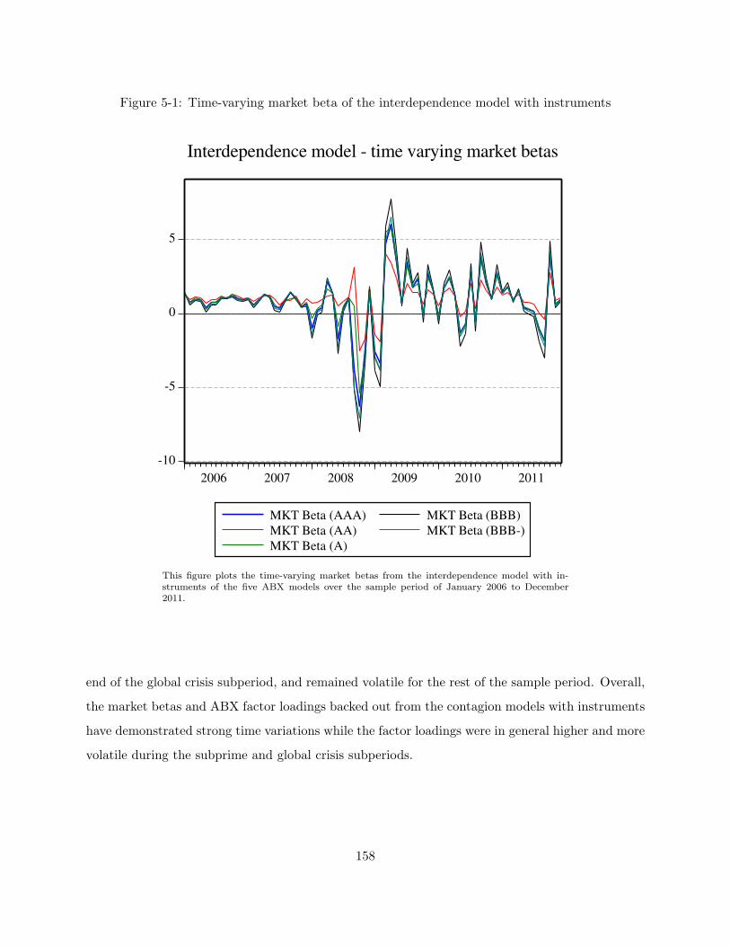
Figure 5-1: Time-varying market beta of the interdependence model with instruments
-10
-5
0
5
2006 2007 2008 2009 2010 2011
MKT Beta (AAA)
MKT Beta (AA)
MKT Beta (A)
MKT Beta (BBB)
MKT Beta (BBB-)
Interdependence model - time varying market betas
This figure plots the time-varying market betas from the interdependence model with in-struments of the five ABX models over the sample period of January 2006 to December2011.
end of the global crisis subperiod, and remained volatile for the rest of the sample period. Overall,
the market betas and ABX factor loadings backed out from the contagion models with instruments
have demonstrated strong time variations while the factor loadings were in general higher and more
volatile during the subprime and global crisis subperiods.
158
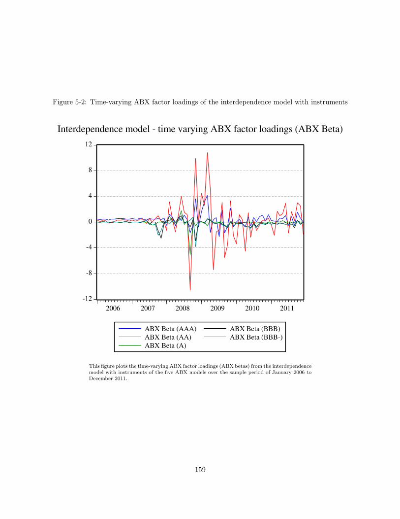
Figure 5-2: Time-varying ABX factor loadings of the interdependence model with instruments
-12
-8
-4
0
4
8
12
2006 2007 2008 2009 2010 2011
ABX Beta (AAA)
ABX Beta (AA)
ABX Beta (A)
ABX Beta (BBB)
ABX Beta (BBB-)
Interdependence model - time varying ABX factor loadings (ABX Beta)
This figure plots the time-varying ABX factor loadings (ABX betas) from the interdependencemodel with instruments of the five ABX models over the sample period of January 2006 toDecember 2011.
159

Contagion model
In this section, I further allow the factor loadings to interact with the contagion related instruments
and the crisis dummy variables. My full contagion model with instruments is shown in Equations 5.1
to 5.4 with the findings reported in Table 5.14.
Consistent with the findings of the contagion models without instruments, the market betas are
all significant across the ABX models despite being smaller in value while the ABX AAA, BBB
and BBB- factor loadings are significant and positive. The coefficients on the TED (ϕMKT,TED)
and Moody’s BAA corporate bond yield spreads (ϕMKT,BAA) are significant and positive, suggest-
ing that the widening of the TED and Moody’s corporate bond yield spreads is associated with
higher market betas during the non-crisis period. In addition, I document significant and negative
ξMKT,TED and ζMKT,TED values, and positive ξMKT,BAA and ζMKT,BAA values in both the ABX
BBB and BBB- models. The positive relation between the changes in corporate bond yield spreads
(in TED spreads) and the level of market systematic risk has become stronger (weaker) during the
crisis. My results suggest that the individual stock market systematic risks are driven by the level
of credit risk and funding illiquidity in the US.
For the ABX factor loadings, significant and negative relations between the ABCP spreads and
the ABX factor loadings (ϕABX,ABCP ) is documented during the tranquil non-crisis period. The
widening of the ABCP spreads is associated with lower ABX factor loadings during the time before
and after the crisis. The instruments interacting with the ABX factor loadings and the subprime
crisis dummy variables (ξABX,TED, ξABX,BAA and ξABX,ABCP ) are highly significant and positive in
the ABX BBB and BBB- models. The TED, Moody’s BAA and ABCP spreads’ negative relation
with the ABX factor loadings has weakened and even become positive during the subprime and
global crisis. In other words, the effects of the contagion variables on the ABX factor loadings
have become more positive and when these spreads widened during the crisis the individual stock’s
exposure to the ABX innovations increased significantly. In addition, I also document significant
and positive relations between the TED spreads and the ABX factor loadings, as well as between
the corporate bond yield spreads and the ABX factor loadings, particularly during the subprime
crisis as evinced by the significant ξABX,TED and ξABX,BAA values in both the ABX BBB and
BBB- models.
Figures 5-3 and 5-4 plot the time-varying market betas and ABX factor loadings associated
160

with the contagion models with instruments, respectively, based on the scaled variables. The plots
of the contagion models are qualitatively similar to those of the interdependence models in that the
market betas fell in mid-2007 and became negative when Lehman Brothers collapsed in September
and October 2008, followed by occasional positive spikes in mid-2009 and negative dips in mid-2010
and the second half of 2011. The ABX factor loadings were volatile and became unreasonably large
during the crisis, which is suggestive of model mis-specification. I observe that the ABX BBB
and BBB- factor loadings turned negative in 2007Q1, jumped to as high as 50.0 in mid-2007 and
peaked in October 2007. Similar to the findings of the independence model, the ABX factor loadings
increased in early and mid-2008 and fell sharply in September and October 2008. The ABX factor
loadings increased sharply again in November 2008 (except for the ABX A factor loadings) and
remained largely volatile over the remaining sample period.
161
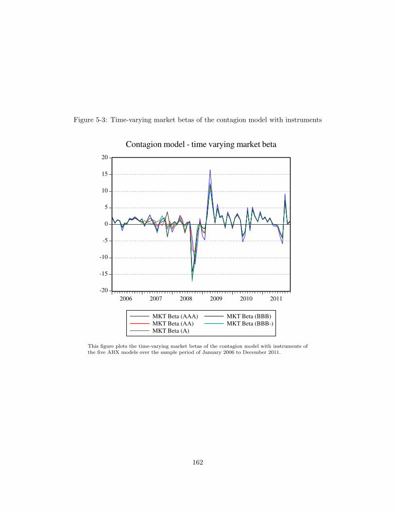
Figure 5-3: Time-varying market betas of the contagion model with instruments
-20
-15
-10
-5
0
5
10
15
20
2006 2007 2008 2009 2010 2011
MKT Beta (AAA)
MKT Beta (AA)
MKT Beta (A)
MKT Beta (BBB)
MKT Beta (BBB-)
Contagion model - time varying market beta
This figure plots the time-varying market betas of the contagion model with instruments ofthe five ABX models over the sample period of January 2006 to December 2011.
162
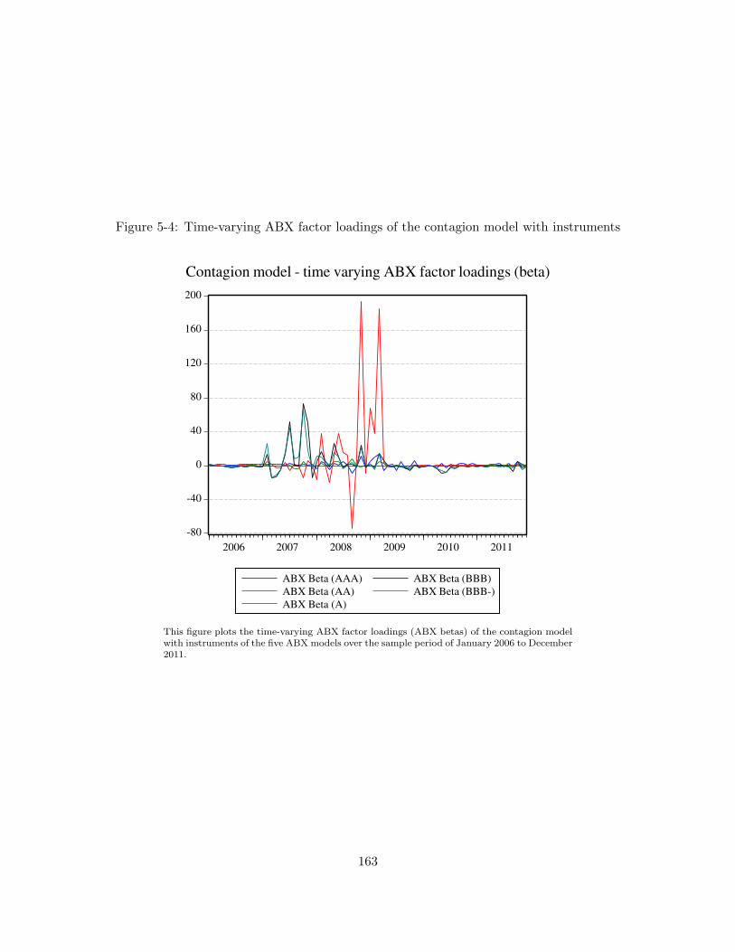
Figure 5-4: Time-varying ABX factor loadings of the contagion model with instruments
-80
-40
0
40
80
120
160
200
2006 2007 2008 2009 2010 2011
ABX Beta (AAA)
ABX Beta (AA)
ABX Beta (A)
ABX Beta (BBB)
ABX Beta (BBB-)
Contagion model - time varying ABX factor loadings (beta)
This figure plots the time-varying ABX factor loadings (ABX betas) of the contagion modelwith instruments of the five ABX models over the sample period of January 2006 to December2011.
163
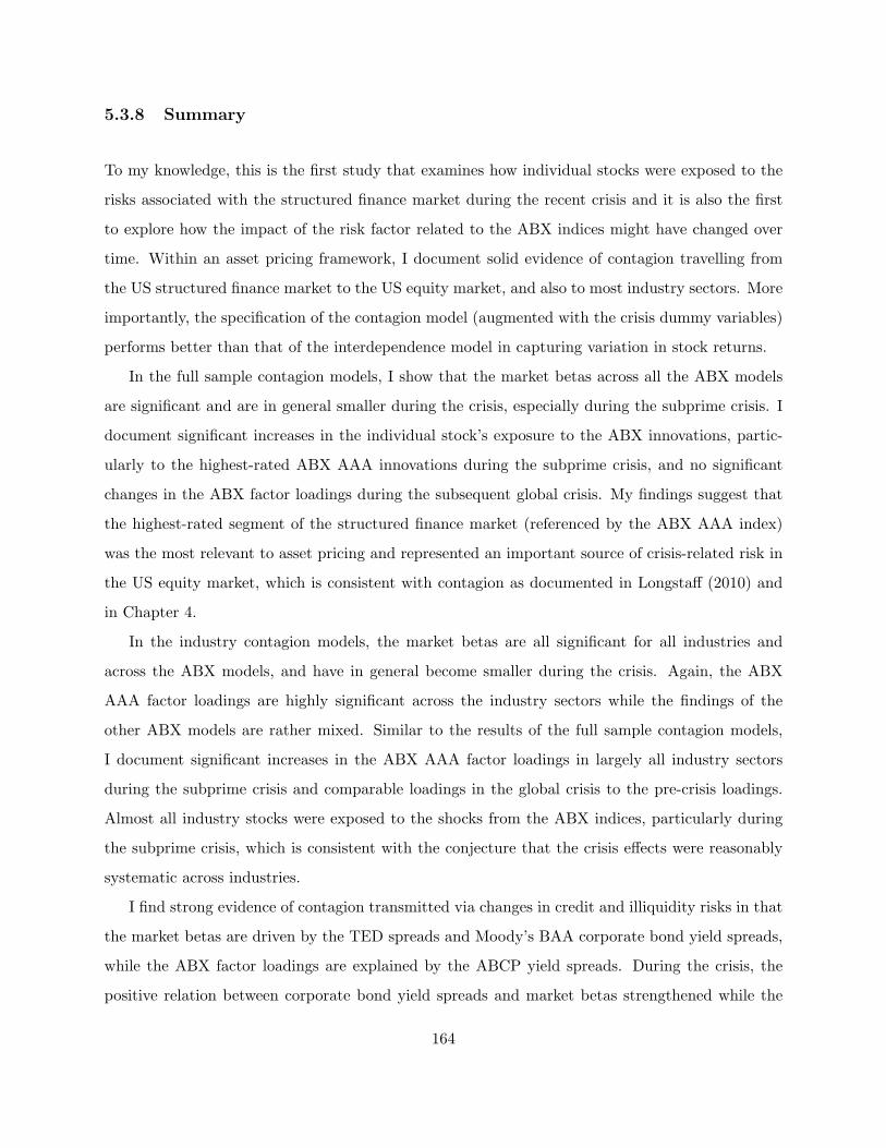
5.3.8 Summary
To my knowledge, this is the first study that examines how individual stocks were exposed to the
risks associated with the structured finance market during the recent crisis and it is also the first
to explore how the impact of the risk factor related to the ABX indices might have changed over
time. Within an asset pricing framework, I document solid evidence of contagion travelling from
the US structured finance market to the US equity market, and also to most industry sectors. More
importantly, the specification of the contagion model (augmented with the crisis dummy variables)
performs better than that of the interdependence model in capturing variation in stock returns.
In the full sample contagion models, I show that the market betas across all the ABX models
are significant and are in general smaller during the crisis, especially during the subprime crisis. I
document significant increases in the individual stock’s exposure to the ABX innovations, partic-
ularly to the highest-rated ABX AAA innovations during the subprime crisis, and no significant
changes in the ABX factor loadings during the subsequent global crisis. My findings suggest that
the highest-rated segment of the structured finance market (referenced by the ABX AAA index)
was the most relevant to asset pricing and represented an important source of crisis-related risk in
the US equity market, which is consistent with contagion as documented in Longstaff (2010) and
in Chapter 4.
In the industry contagion models, the market betas are all significant for all industries and
across the ABX models, and have in general become smaller during the crisis. Again, the ABX
AAA factor loadings are highly significant across the industry sectors while the findings of the
other ABX models are rather mixed. Similar to the results of the full sample contagion models,
I document significant increases in the ABX AAA factor loadings in largely all industry sectors
during the subprime crisis and comparable loadings in the global crisis to the pre-crisis loadings.
Almost all industry stocks were exposed to the shocks from the ABX indices, particularly during
the subprime crisis, which is consistent with the conjecture that the crisis effects were reasonably
systematic across industries.
I find strong evidence of contagion transmitted via changes in credit and illiquidity risks in that
the market betas are driven by the TED spreads and Moody’s BAA corporate bond yield spreads,
while the ABX factor loadings are explained by the ABCP yield spreads. During the crisis, the
positive relation between corporate bond yield spreads and market betas strengthened while the
164

positive relation between the TED spreads and market betas weakened. The evidence suggests
that the market wide default risk is relevant in determining the market betas. For the ABX factor
loadings, during the subprime crisis, the ABX BBB and BBB- factor loadings increased significantly
via the widening of the three yield spreads. During the global crisis, the negative relation between
the ABCP yield spreads and the ABX factor loadings weakened and became positive. The evidence
in this chapter provides additional empirical support to my conjecture that the increased market
linkages between the structured finance and equity markets were closely related to the systematic
funding illiquidity, which is consistent with contagion transmission via the funding liquidity channel.
The evidence also supports the conclusion of Fender and Scheicher (2009), who argue that the falling
ABX prices reflected increasing illiquidity risk and risk aversion during the crisis.
5.4 Do the ABX factors explain the cross-section of expected re-
turns? Evidence based on the daily Fama and French 25 port-
folio returns
In the previous sections, I find evidence that the spillovers of shocks from the ABX AAA index
impacted the US stock returns in a systematic manner and that the ABX factor was important to
asset valuation during the subprime crisis. I will now proceed to explore whether the ABX factors
explain the cross-section of expected returns during the crisis. To this end, a multifactor model
is formulated with k factors following Chen et al. (1986). The expected cross-sectional return of
stock i is assumed to be generated under the following process:
E(Rit) =
k∑j=1
βijλj , (5.14)
where E(Rit) is the expected return of stock i at time t and λj is the price of the jth risk factor.
Empirically, the multifactor model can be tested using a two-pass regression framework following
Black et al. (1972), in which the first pass is a time-series regression and the second pass is a cross-
sectional regression. In the first stage, I obtain estimates of the factor betas on each sorted portfolios
165
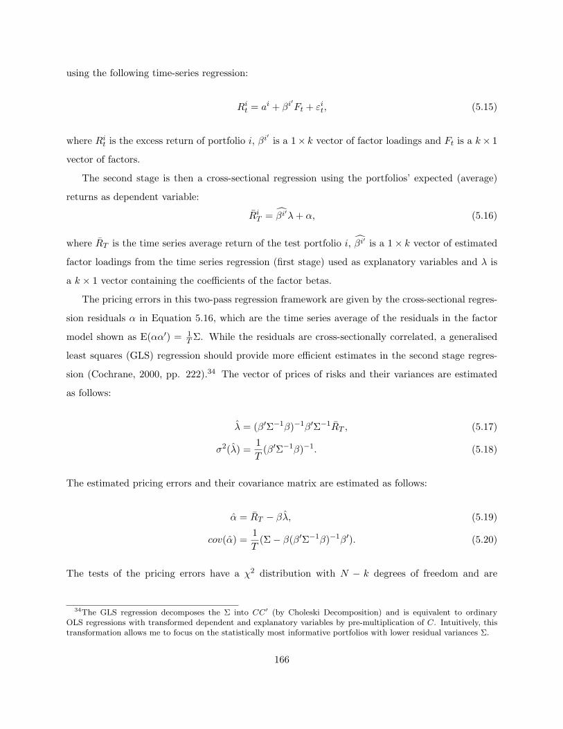
using the following time-series regression:
Rit = ai + βi
′Ft + εit, (5.15)
where Rit is the excess return of portfolio i, βi
′is a 1× k vector of factor loadings and Ft is a k× 1
vector of factors.
The second stage is then a cross-sectional regression using the portfolios’ expected (average)
returns as dependent variable:
RiT = βi′λ+ α, (5.16)
where RT is the time series average return of the test portfolio i, βi′ is a 1× k vector of estimated
factor loadings from the time series regression (first stage) used as explanatory variables and λ is
a k × 1 vector containing the coefficients of the factor betas.
The pricing errors in this two-pass regression framework are given by the cross-sectional regres-
sion residuals α in Equation 5.16, which are the time series average of the residuals in the factor
model shown as E(αα′) = 1T Σ. While the residuals are cross-sectionally correlated, a generalised
least squares (GLS) regression should provide more efficient estimates in the second stage regres-
sion (Cochrane, 2000, pp. 222).34 The vector of prices of risks and their variances are estimated
as follows:
λ = (β′Σ−1β)−1β′Σ−1RT , (5.17)
σ2(λ) =1
T(β′Σ−1β)−1. (5.18)
The estimated pricing errors and their covariance matrix are estimated as follows:
α = RT − βλ, (5.19)
cov(α) =1
T(Σ− β(β′Σ−1β)−1β′). (5.20)
The tests of the pricing errors have a χ2 distribution with N − k degrees of freedom and are
34The GLS regression decomposes the Σ into CC′ (by Choleski Decomposition) and is equivalent to ordinaryOLS regressions with transformed dependent and explanatory variables by pre-multiplication of C. Intuitively, thistransformation allows me to focus on the statistically most informative portfolios with lower residual variances Σ.
166
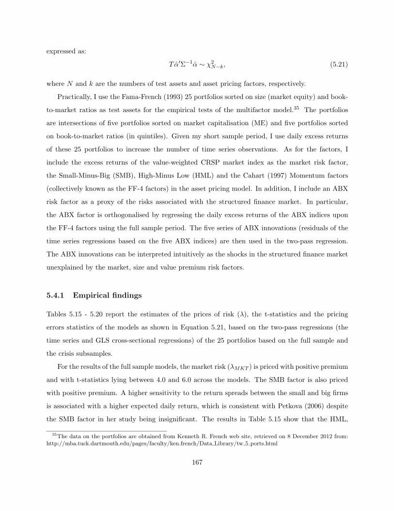
expressed as:
T α′Σ−1α ∼ χ2N−k, (5.21)
where N and k are the numbers of test assets and asset pricing factors, respectively.
Practically, I use the Fama-French (1993) 25 portfolios sorted on size (market equity) and book-
to-market ratios as test assets for the empirical tests of the multifactor model.35 The portfolios
are intersections of five portfolios sorted on market capitalisation (ME) and five portfolios sorted
on book-to-market ratios (in quintiles). Given my short sample period, I use daily excess returns
of these 25 portfolios to increase the number of time series observations. As for the factors, I
include the excess returns of the value-weighted CRSP market index as the market risk factor,
the Small-Minus-Big (SMB), High-Minus Low (HML) and the Cahart (1997) Momentum factors
(collectively known as the FF-4 factors) in the asset pricing model. In addition, I include an ABX
risk factor as a proxy of the risks associated with the structured finance market. In particular,
the ABX factor is orthogonalised by regressing the daily excess returns of the ABX indices upon
the FF-4 factors using the full sample period. The five series of ABX innovations (residuals of the
time series regressions based on the five ABX indices) are then used in the two-pass regression.
The ABX innovations can be interpreted intuitively as the shocks in the structured finance market
unexplained by the market, size and value premium risk factors.
5.4.1 Empirical findings
Tables 5.15 - 5.20 report the estimates of the prices of risk (λ), the t-statistics and the pricing
errors statistics of the models as shown in Equation 5.21, based on the two-pass regressions (the
time series and GLS cross-sectional regressions) of the 25 portfolios based on the full sample and
the crisis subsamples.
For the results of the full sample models, the market risk (λMKT ) is priced with positive premium
and with t-statistics lying between 4.0 and 6.0 across the models. The SMB factor is also priced
with positive premium. A higher sensitivity to the return spreads between the small and big firms
is associated with a higher expected daily return, which is consistent with Petkova (2006) despite
the SMB factor in her study being insignificant. The results in Table 5.15 show that the HML,
35The data on the portfolios are obtained from Kenneth R. French web site, retrieved on 8 December 2012 from:http://mba.tuck.dartmouth.edu/pages/faculty/ken.french/Data Library/tw 5 ports.html
167
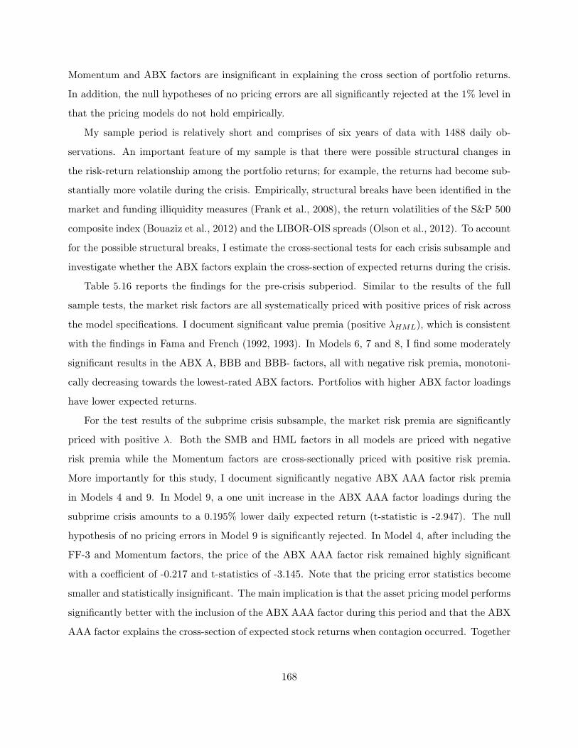
Momentum and ABX factors are insignificant in explaining the cross section of portfolio returns.
In addition, the null hypotheses of no pricing errors are all significantly rejected at the 1% level in
that the pricing models do not hold empirically.
My sample period is relatively short and comprises of six years of data with 1488 daily ob-
servations. An important feature of my sample is that there were possible structural changes in
the risk-return relationship among the portfolio returns; for example, the returns had become sub-
stantially more volatile during the crisis. Empirically, structural breaks have been identified in the
market and funding illiquidity measures (Frank et al., 2008), the return volatilities of the S&P 500
composite index (Bouaziz et al., 2012) and the LIBOR-OIS spreads (Olson et al., 2012). To account
for the possible structural breaks, I estimate the cross-sectional tests for each crisis subsample and
investigate whether the ABX factors explain the cross-section of expected returns during the crisis.
Table 5.16 reports the findings for the pre-crisis subperiod. Similar to the results of the full
sample tests, the market risk factors are all systematically priced with positive prices of risk across
the model specifications. I document significant value premia (positive λHML), which is consistent
with the findings in Fama and French (1992, 1993). In Models 6, 7 and 8, I find some moderately
significant results in the ABX A, BBB and BBB- factors, all with negative risk premia, monotoni-
cally decreasing towards the lowest-rated ABX factors. Portfolios with higher ABX factor loadings
have lower expected returns.
For the test results of the subprime crisis subsample, the market risk premia are significantly
priced with positive λ. Both the SMB and HML factors in all models are priced with negative
risk premia while the Momentum factors are cross-sectionally priced with positive risk premia.
More importantly for this study, I document significantly negative ABX AAA factor risk premia
in Models 4 and 9. In Model 9, a one unit increase in the ABX AAA factor loadings during the
subprime crisis amounts to a 0.195% lower daily expected return (t-statistic is -2.947). The null
hypothesis of no pricing errors in Model 9 is significantly rejected. In Model 4, after including the
FF-3 and Momentum factors, the price of the ABX AAA factor risk remained highly significant
with a coefficient of -0.217 and t-statistics of -3.145. Note that the pricing error statistics become
smaller and statistically insignificant. The main implication is that the asset pricing model performs
significantly better with the inclusion of the ABX AAA factor during this period and that the ABX
AAA factor explains the cross-section of expected stock returns when contagion occurred. Together
168

with the previous results documented in Section 5.3, the negative price of risk of the ABX AAA
factor is consistent with the findings that individual stocks positively correlated with the ABX
innovations had lower returns during the subprime crisis. The empirical evidence confirms my
expectation in that the impact of the spillovers of shocks from the ABX indices on the stock
returns was reasonably systematic and was specific to this subprime crisis subperiod.
The results for the global crisis subsample are reported in Table 5.18. Significant and negative
prices of the market risk and size premia are documented while the price of the momentum premium
is marginally significant and positive. Portfolios with higher market betas had lower expected
returns when the market index declined during the global crisis. On the other hand, all λABX values
are insignificant across the model specifications. One possible explanation is that the structured
finance market was no longer the source of shocks as the crisis went global. In addition, the
informativeness of the ABX indices might have already been reflected in the market index when
the ABX indices received more coverage and attention as an important class of risk barometer at
the onset of the subprime crisis. To my surprise, all pricing error statistics are insignificant in this
period, which is suggestive of good model fit.
As for the post-crisis subperiod, the market risk factors, SMB and Momentum factors are priced
with positive λ. I find that the ABX BBB factor is priced in Models 7 and 12 with significant and
negative prices, respectively. The test results associated with the other ABX factors are somewhat
mixed. The findings are in general consistent with the findings of no significant contagion from
the ABX indices to the equity market during the post-crisis subperiod. The null hypotheses of no
pricing errors are significantly rejected for all model specifications.
I further examine the cross-sectional risk-return relation using observations from both the sub-
prime and global crisis subperiods to test whether the significant price of ABX AAA risk in the
subprime crisis subsample still persists. As shown in Table 5.20, the prices of market risk are all
significant and negative identical to the global crisis subsample results while the HML and momen-
tum factors are priced (negative λHML and positive λMOM values). The λABX associated with all
the ABX factors for all model specifications are in general insignificant. The evidence leads me to
conclude that the ABX AAA factor was priced only during the subprime crisis subperiod and that
the ABX AAA innovations were the most relevant to asset pricing.
To summarise, my full sample tests document little evidence that the ABX factors explain
169
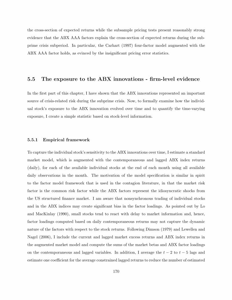
the cross-section of expected returns while the subsample pricing tests present reasonably strong
evidence that the ABX AAA factors explain the cross-section of expected returns during the sub-
prime crisis subperiod. In particular, the Carhart (1997) four-factor model augmented with the
ABX AAA factor holds, as evinced by the insignificant pricing error statistics.
5.5 The exposure to the ABX innovations - firm-level evidence
In the first part of this chapter, I have shown that the ABX innovations represented an important
source of crisis-related risk during the subprime crisis. Now, to formally examine how the individ-
ual stock’s exposure to the ABX innovation evolved over time and to quantify the time-varying
exposure, I create a simple statistic based on stock-level information.
5.5.1 Empirical framework
To capture the individual stock’s sensitivity to the ABX innovations over time, I estimate a standard
market model, which is augmented with the contemporaneous and lagged ABX index returns
(daily), for each of the available individual stocks at the end of each month using all available
daily observations in the month. The motivation of the model specification is similar in spirit
to the factor model framework that is used in the contagion literature, in that the market risk
factor is the common risk factor while the ABX factors represent the idiosyncratic shocks from
the US structured finance market. I am aware that nonsynchronous trading of individual stocks
and in the ABX indices may create significant bias in the factor loadings. As pointed out by Lo
and MacKinlay (1990), small stocks tend to react with delay to market information and, hence,
factor loadings computed based on daily contemporaneous returns may not capture the dynamic
nature of the factors with respect to the stock returns. Following Dimson (1979) and Lewellen and
Nagel (2006), I include the current and lagged market excess returns and ABX index returns in
the augmented market model and compute the sums of the market betas and ABX factor loadings
on the contemporaneous and lagged variables. In addition, I average the t − 2 to t − 5 lags and
estimate one coefficient for the average constrained lagged returns to reduce the number of estimated
170
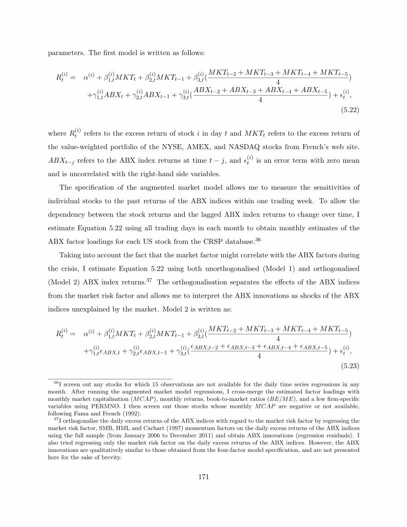
parameters. The first model is written as follows:
R(i)t = α(i) + β
(i)1,tMKTt + β
(i)2,tMKTt−1 + β
(i)3,t(
MKTt−2 +MKTt−3 +MKTt−4 +MKTt−5
4)
+γ(i)1,tABXt + γ
(i)2,tABXt−1 + γ
(i)3,t(
ABXt−2 +ABXt−3 +ABXt−4 +ABXt−5
4) + ϵ
(i)t ,
(5.22)
where R(i)t refers to the excess return of stock i in day t and MKTt refers to the excess return of
the value-weighted portfolio of the NYSE, AMEX, and NASDAQ stocks from French’s web site.
ABXt−j refers to the ABX index returns at time t − j, and ϵ(i)t is an error term with zero mean
and is uncorrelated with the right-hand side variables.
The specification of the augmented market model allows me to measure the sensitivities of
individual stocks to the past returns of the ABX indices within one trading week. To allow the
dependency between the stock returns and the lagged ABX index returns to change over time, I
estimate Equation 5.22 using all trading days in each month to obtain monthly estimates of the
ABX factor loadings for each US stock from the CRSP database.36
Taking into account the fact that the market factor might correlate with the ABX factors during
the crisis, I estimate Equation 5.22 using both unorthogonalised (Model 1) and orthogonalised
(Model 2) ABX index returns.37 The orthogonalisation separates the effects of the ABX indices
from the market risk factor and allows me to interpret the ABX innovations as shocks of the ABX
indices unexplained by the market. Model 2 is written as:
R(i)t = α(i) + β
(i)1,tMKTt + β
(i)2,tMKTt−1 + β
(i)3,t(
MKTt−2 +MKTt−3 +MKTt−4 +MKTt−5
4)
+γ(i)1,tϵABX,t + γ
(i)2,tϵABX,t−1 + γ
(i)3,t(
ϵABX,t−2 + ϵABX,t−3 + ϵABX,t−4 + ϵABX,t−5
4) + ϵ
(i)t ,
(5.23)
36I screen out any stocks for which 15 observations are not available for the daily time series regressions in anymonth. After running the augmented market model regressions, I cross-merge the estimated factor loadings withmonthly market capitalisation (MCAP ), monthly returns, book-to-market ratios (BE/ME), and a few firm-specificvariables using PERMNO. I then screen out those stocks whose monthly MCAP are negative or not available,following Fama and French (1992).
37I orthogonalise the daily excess returns of the ABX indices with regard to the market risk factor by regressing themarket risk factor, SMB, HML and Carhart (1997) momentum factors on the daily excess returns of the ABX indicesusing the full sample (from January 2006 to December 2011) and obtain ABX innovations (regression residuals). Ialso tried regressing only the market risk factor on the daily excess returns of the ABX indices. However, the ABXinnovations are qualitatively similar to those obtained from the four-factor model specification, and are not presentedhere for the sake of brevity.
171
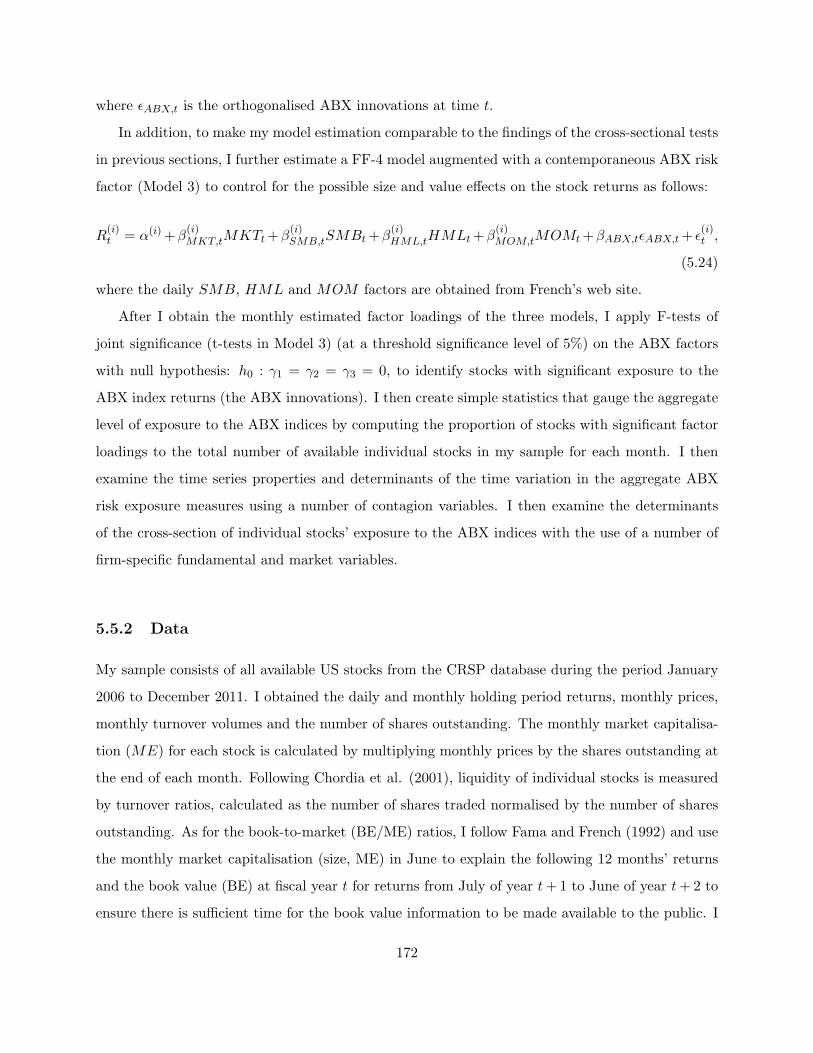
where ϵABX,t is the orthogonalised ABX innovations at time t.
In addition, to make my model estimation comparable to the findings of the cross-sectional tests
in previous sections, I further estimate a FF-4 model augmented with a contemporaneous ABX risk
factor (Model 3) to control for the possible size and value effects on the stock returns as follows:
R(i)t = α(i)+β
(i)MKT,tMKTt+β
(i)SMB,tSMBt+β
(i)HML,tHMLt+β
(i)MOM,tMOMt+βABX,tϵABX,t+ ϵ
(i)t ,
(5.24)
where the daily SMB, HML and MOM factors are obtained from French’s web site.
After I obtain the monthly estimated factor loadings of the three models, I apply F-tests of
joint significance (t-tests in Model 3) (at a threshold significance level of 5%) on the ABX factors
with null hypothesis: h0 : γ1 = γ2 = γ3 = 0, to identify stocks with significant exposure to the
ABX index returns (the ABX innovations). I then create simple statistics that gauge the aggregate
level of exposure to the ABX indices by computing the proportion of stocks with significant factor
loadings to the total number of available individual stocks in my sample for each month. I then
examine the time series properties and determinants of the time variation in the aggregate ABX
risk exposure measures using a number of contagion variables. I then examine the determinants
of the cross-section of individual stocks’ exposure to the ABX indices with the use of a number of
firm-specific fundamental and market variables.
5.5.2 Data
My sample consists of all available US stocks from the CRSP database during the period January
2006 to December 2011. I obtained the daily and monthly holding period returns, monthly prices,
monthly turnover volumes and the number of shares outstanding. The monthly market capitalisa-
tion (ME) for each stock is calculated by multiplying monthly prices by the shares outstanding at
the end of each month. Following Chordia et al. (2001), liquidity of individual stocks is measured
by turnover ratios, calculated as the number of shares traded normalised by the number of shares
outstanding. As for the book-to-market (BE/ME) ratios, I follow Fama and French (1992) and use
the monthly market capitalisation (size, ME) in June to explain the following 12 months’ returns
and the book value (BE) at fiscal year t for returns from July of year t+ 1 to June of year t+2 to
ensure there is sufficient time for the book value information to be made available to the public. I
172

also estimate the idiosyncratic volatilities (IV ol) for each individual stock with a similar approach
to recent studies (see, for example, Ang et al., 2006, 2009; Fu, 2009). I compute the IV ol as
the standard deviation of the regression residuals of my models in Equation 5.22 - 5.24. I then
transform the daily IV ol measure into a 30-day equivalent measure by multiplying the volatility
measure by the square root of 30 to obtain the 30-day or pseudo monthly IV ol measure for each
individual stock.38
Similar to the empirical analysis in Chapter 4, I omit the daily observations between 1 April and
31 August 2009 because the prices of both the ABX BBB and BBB- indices were stale, causing near-
singularity problems in ordinary regressions. Therefore, the post-crisis subperiod for the current
analysis starts from 1 September 2009 and lasts until the end of 2011.
5.5.3 Univariate analysis - decile sort portfolios
After the monthly estimates of factor loadings are obtained, I perform univariate portfolio analysis
sorted by the ABX factor loadings to address two research objectives: i) to investigate the cross-
sectional determinants of individual stocks’ exposure to the ABX indices; and, ii) to test whether
the ABX factors explain the cross-sectional variations in portfolio returns as a robustness check to
Section 5.4. Practically, I sort the stocks into decile portfolios at the end of each month immediately
after estimating the models. Stocks are allowed to move across portfolios through time while
maintaining the portfolio’s relative ABX factor loadings. I report two sets of portfolio sort results
based on two sample selection approaches. In the former approach, the sorts are based on the ABX
factor loadings on all available stocks while the second method sorts only stocks with significant
test statistics (at 5% significance level) to allow me to focus more closely on those stocks with
significant exposure. The equally weighted average characteristics of the deciles portfolios (which
includes market capitalisation, turnover ratios, month t returns, month t + 1 returns, standard
deviations, idiosyncratic volatilities, α, market betas, and the ABX factor loadings) are reported,
grouped by crisis subperiods.
Tables 5.21 - 5.25 report the equally weighted average characteristics of the deciles portfolios
sorted by the sums of ABX factor loadings of Model 1 based on all available stocks and the
unorthogonalised ABX AAA, AA, A, BBB and BBB- index returns, respectively. A number of
38A similar approach has been adopted by French et al. (1987) and Fu (2009).
173
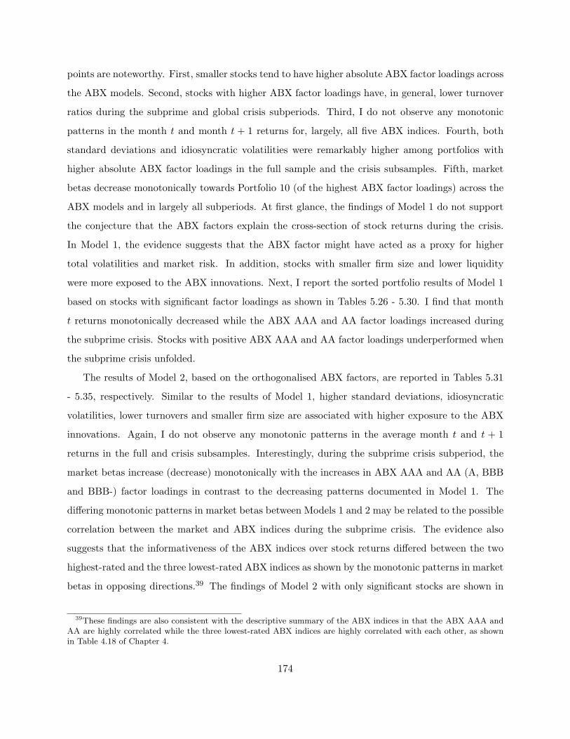
points are noteworthy. First, smaller stocks tend to have higher absolute ABX factor loadings across
the ABX models. Second, stocks with higher ABX factor loadings have, in general, lower turnover
ratios during the subprime and global crisis subperiods. Third, I do not observe any monotonic
patterns in the month t and month t + 1 returns for, largely, all five ABX indices. Fourth, both
standard deviations and idiosyncratic volatilities were remarkably higher among portfolios with
higher absolute ABX factor loadings in the full sample and the crisis subsamples. Fifth, market
betas decrease monotonically towards Portfolio 10 (of the highest ABX factor loadings) across the
ABX models and in largely all subperiods. At first glance, the findings of Model 1 do not support
the conjecture that the ABX factors explain the cross-section of stock returns during the crisis.
In Model 1, the evidence suggests that the ABX factor might have acted as a proxy for higher
total volatilities and market risk. In addition, stocks with smaller firm size and lower liquidity
were more exposed to the ABX innovations. Next, I report the sorted portfolio results of Model 1
based on stocks with significant factor loadings as shown in Tables 5.26 - 5.30. I find that month
t returns monotonically decreased while the ABX AAA and AA factor loadings increased during
the subprime crisis. Stocks with positive ABX AAA and AA factor loadings underperformed when
the subprime crisis unfolded.
The results of Model 2, based on the orthogonalised ABX factors, are reported in Tables 5.31
- 5.35, respectively. Similar to the results of Model 1, higher standard deviations, idiosyncratic
volatilities, lower turnovers and smaller firm size are associated with higher exposure to the ABX
innovations. Again, I do not observe any monotonic patterns in the average month t and t + 1
returns in the full and crisis subsamples. Interestingly, during the subprime crisis subperiod, the
market betas increase (decrease) monotonically with the increases in ABX AAA and AA (A, BBB
and BBB-) factor loadings in contrast to the decreasing patterns documented in Model 1. The
differing monotonic patterns in market betas between Models 1 and 2 may be related to the possible
correlation between the market and ABX indices during the subprime crisis. The evidence also
suggests that the informativeness of the ABX indices over stock returns differed between the two
highest-rated and the three lowest-rated ABX indices as shown by the monotonic patterns in market
betas in opposing directions.39 The findings of Model 2 with only significant stocks are shown in
39These findings are also consistent with the descriptive summary of the ABX indices in that the ABX AAA andAA are highly correlated while the three lowest-rated ABX indices are highly correlated with each other, as shownin Table 4.18 of Chapter 4.
174

Tables 5.36 - 5.40. The portfolio characteristics remain qualitatively similar while the patterns of
the market betas are more distinctive.
So far, the multifactor models of Model 1 and Model 2 include both the market risk factor and
the ABX risk factor and their lagged terms. In Model 3, I further include the SMB, HML and the
momentum factors and report the equally-weighted average portfolio characteristics in Tables 5.41
- 5.45, respectively. Regarding the firm size, turnover ratios, standard deviations and idiosyncratic
volatilities, the results of Model 3 are, in general, identical to those of Models 1 and 2. I find a
weak and monotonically decreasing pattern in month t returns for the ABX AAA and AA factor
loadings during the subprime crisis. Note that the patterns occur largely during the subprime
crisis; that is, the spillover of shocks from the ABX indices has impacted on the US equity market
in a systematic way. The monotonic patterns largely disappeared in the subsequent subperiods,
which is consistent with my results in Section 5.4. The month t+1 returns are lowest in Portfolios
1 and 10 for all five ABX indices during the subprime crisis. Although the evidence suggests
some return predictability in the ABX factor loadings during the subprime crisis, the relationship
between the ABX factor loadings and the one-month ahead returns is not linear. These findings
are consistent with my contention that the ABX factor loadings are proxies for return volatilities
and, thus, underperformed during the subprime crisis. In addition, the market betas increase
monotonically with the ABX AAA, AA and A factor loadings during the subprime crisis while
the pattern no longer exist during the global and post-crisis subperiods. The results of Model 3
based on stocks with significant ABX factor loadings are reported in Tables 5.46 - 5.50. Similarly,
the month t returns decreased monotonically during the subprime crisis in largely all ABX models
(more prominently in the ABX AAA and AA models). I also find monotonically increasing market
betas across the portfolios during the subprime crisis for all ABX models except the ABX BBB
model. The evidence suggests that, even after controlling for the SMB, HML and the momentum
factors, the ABX factors still explain the cross-section of expected returns during the subprime
crisis.
Note that the findings based on the unorthogonalised and orthogonalised ABX factors differ
substantially, as evinced by the opposing monotonic patterns in the average market betas. Since I
focus on the individual stock’s exposure to the spillover of shocks from the structured finance mar-
ket, empirical analyses based on the orthogonalised ABX factors are more intuitive and appropriate
175
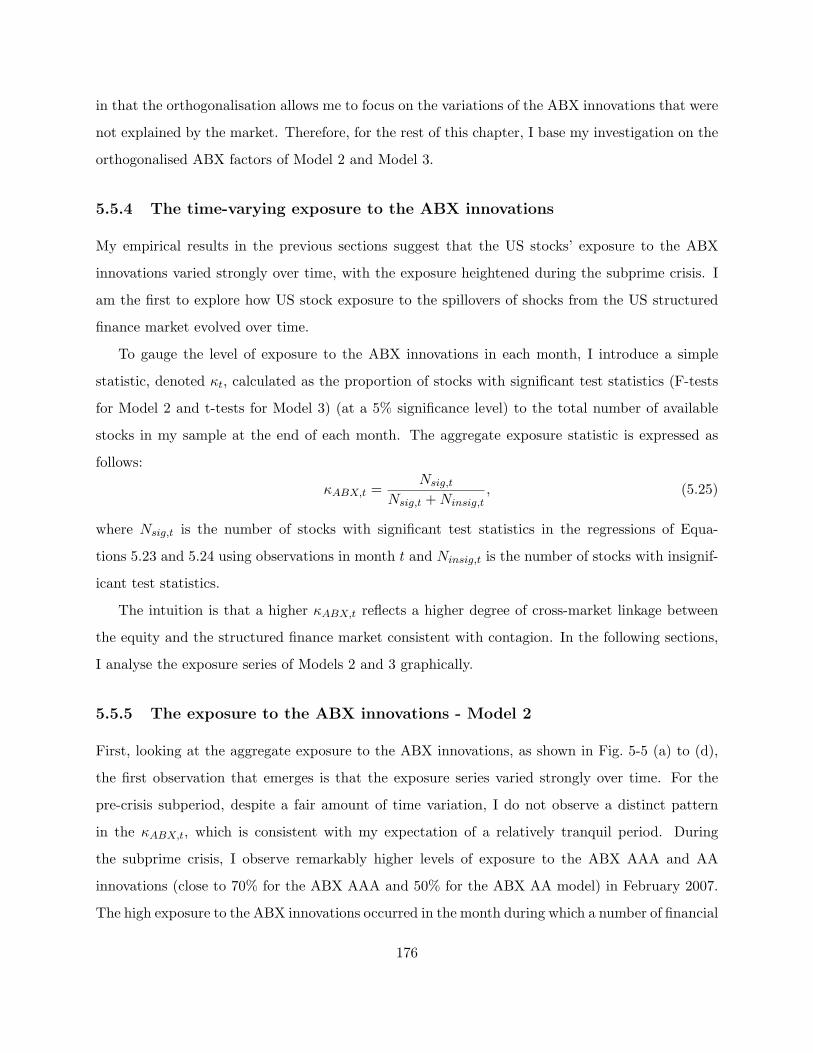
in that the orthogonalisation allows me to focus on the variations of the ABX innovations that were
not explained by the market. Therefore, for the rest of this chapter, I base my investigation on the
orthogonalised ABX factors of Model 2 and Model 3.
5.5.4 The time-varying exposure to the ABX innovations
My empirical results in the previous sections suggest that the US stocks’ exposure to the ABX
innovations varied strongly over time, with the exposure heightened during the subprime crisis. I
am the first to explore how US stock exposure to the spillovers of shocks from the US structured
finance market evolved over time.
To gauge the level of exposure to the ABX innovations in each month, I introduce a simple
statistic, denoted κt, calculated as the proportion of stocks with significant test statistics (F-tests
for Model 2 and t-tests for Model 3) (at a 5% significance level) to the total number of available
stocks in my sample at the end of each month. The aggregate exposure statistic is expressed as
follows:
κABX,t =Nsig,t
Nsig,t +Ninsig,t, (5.25)
where Nsig,t is the number of stocks with significant test statistics in the regressions of Equa-
tions 5.23 and 5.24 using observations in month t and Ninsig,t is the number of stocks with insignif-
icant test statistics.
The intuition is that a higher κABX,t reflects a higher degree of cross-market linkage between
the equity and the structured finance market consistent with contagion. In the following sections,
I analyse the exposure series of Models 2 and 3 graphically.
5.5.5 The exposure to the ABX innovations - Model 2
First, looking at the aggregate exposure to the ABX innovations, as shown in Fig. 5-5 (a) to (d),
the first observation that emerges is that the exposure series varied strongly over time. For the
pre-crisis subperiod, despite a fair amount of time variation, I do not observe a distinct pattern
in the κABX,t, which is consistent with my expectation of a relatively tranquil period. During
the subprime crisis, I observe remarkably higher levels of exposure to the ABX AAA and AA
innovations (close to 70% for the ABX AAA and 50% for the ABX AA model) in February 2007.
The high exposure to the ABX innovations occurred in the month during which a number of financial
176
institutions revealed troubles relating to their subprime mortgage businesses40, following which the
ABX indices started to decline sharply. In addition, I observe a moderately high level of exposure
in July and October 2007, again coinciding with a number of distress events and bankruptcies
among financial institutions41 and surging funding illiquidity in the US financial system.42 As the
crisis evolved into a global context, the exposure to the ABX innovations heightened in 2008Q1
and 2008Q4 after the Lehman Brothers collapse. During the post-crisis subperiod, I still observe
a fair amount of volatility in the exposure series but I find lower correlation among the five ABX
exposure series, suggesting that the common factors that drove the stock markets’ exposure to the
structured finance market might no longer exist.
Next, I analyse and discuss the exposure series that are grouped according to the signs of
exposure43 as shown in Fig. 5-7 (a) to (h). The exposure series to the ABX innovations are
qualitatively similar to those without grouping by sign. During the subprime crisis, both the
positive and negative exposure series heightened in February 2007. In addition, in July 2007 and
2007Q4, I observe a higher level of positive exposure than negative exposure in that more stocks
have comoved positively with the ABX innovations consistent with contagion. During the global
crisis subperiod, the exposure to the ABX innovation was most considerable in 2008Q1 and 2008Q4.
The maximal exposure to the ABX innovations was attained shortly after the collapse of Lehman
Brothers. As for the post-crisis subperiod, I still observe reasonably strong time variations in the
stocks’ exposure, with spikes in the positive exposure series in August 2011.
40Some of these troubled institutions include various subprime mortgage lenders; for example, Ownit MortgageSolutions Inc. (in January 2007), Mortgage Lenders Network USA Inc. (in January 2007) (Cox and Glapa, 2009),American Freedom Mortgage Inc. (filed Chapter 7 for liquidation on the 30th January 2007) and ResMae MortgageCorp. (filed Chapter 11 in February 2007 as the 26th largest subprime mortgage lender). On the 22 February 2007,HSBC announced a surprise increase in bad debt provision for 2006 and fired the head of their subprime mortgagebusinesses, who was responsible for a loss of $10.5 billion (BBC News). On the 27 February 2007, the Federal HomeLoan Mortgage Corporation (Freddie Mac) stated that it would not buy the most risky subprime mortgages andmortgage-related securities (Federal Reserve Bank of St. Louis).
41As the subprime crisis substantiated, a number of financial institutions suffered significant write-downs andbankruptcies, as follows: Deutsche Bank ($3.0 billion write-down on bad debts in October 2007), UBS ($3.7 billionwrite-down in September 2007), Merrill Lynch ($7.9 billion exposure to bad debts in October 2007), Citigroup ($5.9billion write-down on bad debts), Nomura (closed down subprime mortgage division and suffered $621 million losses)and Bank of China ($9 billion losses in subprime businesses in September 2007), etc.
42As shown in Figure 5.7, both the Moody’s BAA corporate bond and the ABCP yield spreads started to widenfrom August 2007 onwards. The heightening threat of insolvency hit the overnight lending market (LIBOR reached6.75%) and the liquidity in the money market quickly dried up in early September 2007 (BBC News). The EuropeanCentral Bank also expressed concern about funding illiquidity in the money markets as a result of the troubles in thesubprime mortgage market, as reflected by the widening EURIBOR (ECB Timeline of the financial crisis).
43The direction of exposure is determined by the signs of the significant ABX factor loadings.
177
5.5.6 The exposure to the ABX innovations - Model 3
To check the robustness of the above results, I estimate Model 3 of Equation 5.24 for each indi-
vidual stock and compute the κABX,t as explained in Section 5.5.4. Note that Model 3 is different
from Model 2 in two major ways. First, Model 3 includes only the contemporaneous regressors
while Model 2 contains both contemporaneous and lagged regressors. Therefore, F-tests of joint
significance are estimated on the contemporaneous and lagged ABX factors in Model 2, while t-
tests on the contemporaneous ABX factor are used in Model 3 to compute the exposure series.
Second, Model 3 controls for the size, value, and momentum effects, and allows me to focus on the
incremental explanatory power of the ABX factors.
Fig. 5-8 (a) to (d) plot the κABX,t of the five ABX indices in each crisis subperiod, respectively.
First, I find that the κABX,t of Model 3 are in general lower than those of Model 2 throughout
the sample period. The observation suggests that the FF-3 factors and momentum factor might
have significant explanatory power over the individual stock’s returns and, hence, the ABX factor
loadings in Model 3 have become less significant. On the other hand, it also suggests the explanatory
power in the lagged market and ABX index returns over the individual stocks’ returns is not
captured. During the subprime crisis, the US stock market experienced substantially higher level
of exposure to the ABX innovations in February 2007, consistent with Model 2. In addition, I
observe peaks in exposure in February, August and November 2008 during the global crisis. The
κABX,t values sorted by exposure direction, as shown in Fig. 5-9 (a) to (h), are qualitatively similar
to those of Model 2, in which a higher level of exposure to the ABX innovations is identified in
February 2007, February, August and November 2008.
5.5.7 Discussions
The graphical analysis demonstrates strong time variations in the individual stock’s exposure to
the ABX innovations throughout my sample period. I find remarkably higher levels of exposure
to the ABX innovations in February, August and October 2007, during the subprime crisis, and
in February, August and November 2008, during the global crisis. The noticeable increases in the
level of ABX exposure during the subprime crisis are consistent with the significant increases in
cross-market linkages between the US equity and structured finance markets, as documented by
Longstaff (2010) and in Chapter 4. The simple statistics associated with the ABX exposure are
178
robust to an alternative model specification that controls for the size, value and momentum effects
and are qualitatively similar between Models 2 and 3.
5.5.8 Granger-causality tests of the κABX,t
In this section, I am interested in the determinants of the time variation in the κABX,t. To this end,
I estimate a VAR model on the monthly κABX,t, with a few well-acknowledged contagion variables,
and test for Granger-causality. Since my findings of significant contagion are concentrated in the
ABX AAA model, I report the results of the κABX,t for the ABX AAA model only. My VAR(1)
model with n endogenous variables is written as:44
yt = αt +A1yt−1 + εt, (5.26)
where yt is a n × 1 vector of endogenous variables, A1 is a n × n matrix of coefficients of the
endogenous variables, and εt is a n×1 vector of errors uncorrelated to the right hand side variables.
A few contagion variables, which are correlated with the heightening credit risk levels, and mar-
ket and funding illiquidity in the US financial system, are included in the VAR model. These vari-
ables include (level data) the TED spreads, ABCP spreads, Moody’s BAA - 10 Year constant matu-
rity yield spreads (BAA), LIBOR-OIS spreads45, the average market illiquidity (AILLIQ) following
Amihud (2002), and the monthly value-weighted average idiosyncratic volatilities (VWIV ol).46
Granger-causality test results
The F-statistics and the corresponding p-values (in squared brackets) associated with the Granger-
causality tests are reported in Table 5.53.
First, I find that κABX,t is Granger-caused by the lagged average market illiquidity, LIBOR-
OIS spreads and average idiosyncratic volatilities. The coefficients on the AILLIQ and LIBOR-
OIS spreads are negative while the coefficient on VWIV ol is positive. Increases in the average
idiosyncratic risks translated into higher one-month ahead stocks’ exposure to the ABX innovations.
44The first-order lag structure is found to best fit the data as shown by the minimum Schwarz Information Criterion(SIC).
45The LIBOR-OIS spread is the yield differential between the LIBOR and the overnight indexed swap rate.46The summary statistics and correlation matrix of the monthly contagion variables are reported in Tables 5.51
and 5.52, respectively. For a detailed description of the contagion variables, please refer to Appendix A.1.
179
To my surprise, higher market and funding illiquidity in the last month is associated with lower
ABX exposure.
Second, the average market illiquidity is driven by the ABCP and LIBOR-OIS spreads with
positive relations and by the TED spreads with a negative relation. The findings are consistent
with Brunnermeier and Pedersen (2009) in that market illiquidity was positively related to funding
illiquidity.
Third, the LIBOR-OIS, TED, and ABCP spreads were relatively more exogenous to the
contagion variables and were in general not explained by the endogenous variables. The Moody’s
BAA corporate bond yield spreads were predicted by the ABCP , LIBOR-OIS (positive relation)
and TED spreads (negative relation), respectively. The VAR model results suggest that the height-
ening market wide default risks were related to the exogenous shocks to funding liquidity in the
previous month. In addition, the average idiosyncratic volatilities were driven positively by the
ABCP , LIBOR-OIS spreads and the AILLIQ. Higher market wide average firm-specific risks
were related significantly to past increases in the market and funding illiquidity and insolvency
risks.
5.6 Determinants of individual stock’s exposure to the ABX in-
novations
In the following sections, I investigate the cross-sectional determinants of an individual stock’s sig-
nificant exposure to the ABX innovations using a diverse set of firm-specific fundamental variables.
The significance of the stock’s ABX exposure is determined by the t-statistics of the ABX factor
in Equation 5.24 (Model 3) at a 5% significance level.47 I obtained the firm-specific fundamental
variables from Compustat and merge the accounting data with the asset-pricing factor loadings
using CUSIP.48
47Although my previous analysis shows that the lagged ABX factors of Model 2 might explain in part stock returns,the complex lag structure inevitably introduces noise in the findings. In addition, the absence of the FF-3 factorsand the Carhart (1997) momentum factor may be inappropriate. To make the findings comparable to previous assetpricing tests and control for the pricing anomalous effects, the empirical analysis in the following sections are basedon Model 3’s specification.
48CUSIP is a unique identifier for a financial security in North America for the purposes of facilitating clearing andsettlement of trades.
180
5.6.1 Asset pricing factors and dependent variables
The asset pricing factor loadings are obtained by estimating the augmented four-factor model of
Equation 5.24 using all daily observations in each crisis subperiod. Two categorical variables,
SIG, whose value is 1 if the stock has a significant t-statistic (p <= 0.05) and zero otherwise,
and SIGN , whose value is 1 if the stock has a significant t-statistic (p <= 0.05) and a positive
ABX factor loading (βABX > 0), 2 if the stock with a significant t-statistic (p <= 0.05) has a
negative ABX factor loading (βABX < 0), and zero otherwise, are included. A set of logistic and
multinomial logistic regressions using SIG and SIGN as dependent variables are estimated to
identify the significant determinants. I also estimate multivariate regressions using the ABX factor
loadings (βABX) as dependent variables to test the relation between the exposure to the ABX
innovation and the fundamental characteristics at a firm level. To mitigate the problematic effects
caused by outliers, I winsorise each independent variable at a 90% level (5% at each tail) to reduce
cross-sectional variations.49
5.6.2 Firm-specific variables
Since there is little theoretical explanation as to which firm-specific characteristics may explain the
cross-section of individual stock’s exposure to the ABX innovations, my investigation is of an ex-
ploratory nature. In addition, because the evidence presented in the previous sections suggests that
the ABX factor loadings might have been a proxy for the increasing total and idiosyncratic volatil-
ities, my investigation is centered on a diverse set of fundamental variables that are empirically
important in explaining the individual stock’s return volatilities.
Firm-specific variables are computed from the balance sheet, income statement and cash flow
statement data items from the Compustat database of annual updates. I use Datadate in the
Compustat as the basis of data inclusion and assume that the fundamental financial information
are made available to the public within four months. For instance, if I estimate the model in
December of year t, I include data from firms with fiscal ending dates within the period September
of year t− 1 to August of year t. Regardless of whether the subperiod is longer or shorter than one
49I experimented with other levels of winsorisation, first with 0.5% at each tail, 1% at each tail and then 5% at eachtail. The levels of winsorisation have had little effect on my findings. I also checked the outcome of the winsorisationusing summary statistics and box plots, and find that the winsorisation at 5% gives a more reasonable cross-sectionaldispersion.
181
year, the same approach is followed.
Profitability and growth variables
Pastor and Veronesi (2003) find that increasing uncertainty in a firm’s profitability explains the
increases in the stock’s average idiosyncratic volatilities. Rajgopal and Venkatachalam (2011) find
that deteriorating earning qualities are associated with higher idiosyncratic volatilities. In a broad
sense, individual firm’s profitability and earnings may have a considerable negative impact on
stock return volatilities. Since the ABX factor might have represented a portion of idiosyncratic
volatilities, I expect that lower profitability and earnings are related to higher exposure to the
ABX innovations. To measure a firm’s profitability and growth rates, I include the earning-yield
(Earn yield), annual percentage changes in sales (Sales growth) and the annual changes in earn-
ings before interests, taxes, depreciation and amortisation (EBITDA), which are normalised by
total assets (EBITDA growth). In addition, I include the amount of capital expenditure as a
fraction of total assets (CAPX AT ) as a measure of growth orientation.
Leverage variables
Schwert (1989) finds that, when firms issue more debt relative to their original capital structure (i.e.
increases in aggregate financial leverage), the return volatilities of the market portfolio increase.
Christie (1982) finds that stock return variances are positively associated with both financial lever-
age and interest rates. One common explanation is that the declines in stock prices lead to a firm’s
higher leverage and, in turn, results in a firm’s higher equity and stock return volatilities. I expect
that firms with higher amounts of total debt have higher return volatilities and are more subject to
the spillovers of shocks from the structured finance market. For the leverage measures (Leverage),
I divide the total debts by total assets.50
Balance sheet liquidity variables
Titman et al. (2004) find that increases in a firm’s investment result in lower subsequent stock
returns. Richardson (2006) argues that the lower future stock returns are related to the over-
investments concentrated in firms with the highest level of free cash flow. Taken together, a better
50The total debts are calculated by adding preferred stock to total liability less any convertible debt and deferredtax liabilities if available.
182
liquidity position (more free cash flow) translates into lower future returns. On the other hand,
Irvine and Pontiff (2008) find that the idiosyncratic volatilities in fundamental cash flows have
increased substantially and are correlated positively with the increases in a stock’s idiosyncratic
volatilities over time. In addition, firms with less free balance sheet liquidity may rely more on
debt financing and have higher equity volatilities and return volatilities. In that sense, I expect a
negative relation between a firm’s cash flow liquidity position and exposure to the ABX innovations.
I measure an individual firm’s balance sheet liquidity position by computing the total amount of
free cash flow normalised by total assets (FCF AT ) in which the free cash flows are calculated by
subtracting the total capital expenditures (CAPX) from the total operating cash flows (OCF ).
Other variables
I include the dividend yields (Div yield) of individual firms and a BIG4 dummy variable in the
analysis.51 Pastor and Veronesi (2003) have documented empirical evidence that firms with no
dividends have higher return volatilities, which is consistent with their theoretical prediction. I
expect firms with lower dividend yields to have higher exposure to the crisis-related shocks. In
addition, the BIG4 dummy variable is a proxy for better earning quality since firms audited by
the BIG4 auditors should have more reliable and accurate information, and are expected to be
negatively related to the ABX exposure.
5.6.3 MCAP, BE/ME, turnover, risks, returns, and other variables
The time-series average log market capitalisation (LN MCAP ), log book-to-market ratios (LN BE/ME)
and log turnover ratios (LN TURN) over the crisis subperiods are included. A few risk measures,
including the standard deviations (Stdev, of the daily returns in each crisis subperiod) and idiosyn-
cratic volatilities (IV ol, see Section 5.5.2) are included while the time series average (over each
crisis subperiod) excess monthly returns of the individual stocks are also included.
5.6.4 Empirical results
Tables 5.54 to 5.58 report the results of the logistic, multinomial logistic and multivariate cross-
sectional regressions of the ABX AAA, AA, A, BBB and BBB- indices, respectively. The estimated
51The BIG4 dummy variable is 1 when the individual firm has been audited with a BIG4 accounting firm duringthe data year, and 0 otherwise.
183

coefficients, t-statistics based on robust standard errors clustered by the 12-industry SIC, the
number of observations, Pseudo R2 (for logistic regressions), and adjusted R2 are reported grouped
by crisis subperiods. In each table, Panel A reports the findings of the logistic regressions, Panels
B and C report the findings of the multinomial logistic regressions based on the model SIGN = 1
(positive ABX exposure) and SIGN = 2 (negative ABX exposure) respectively, and Panel D
reports the findings of the multivariate regressions using βABX as dependent variables.
The ABX AAA index
Given the findings of significant increases in ABX AAA factor loadings during the subprime crisis,
I focus my attention on reporting and discussing the results of the ABX AAA models.
First, the findings of the logistic regressions are qualitatively similar across the ABX indices.
In Table 5.54, my results (Panel A) show that higher standard deviations and lower idiosyncratic
volatilities are associated with higher probabilities of having significant ABX factor loadings in all
crisis subperiods. In addition, stocks with lower market betas are more likely to have significant
ABX factor loadings during the global crisis subperiod.
Next, I split the samples into two groups according to the signs of the ABX factor loadings,
as defined by the SIGN variable, and report the multinomial logistic regression results in Panel
B and C. First, the significant findings in the standard deviations and idiosyncratic volatilities in
Panel A were largely dominated by the model of negative ABX exposure (SIGN = 2 of Panel
C). In Panel B, higher idiosyncratic volatilities and lower standard deviations are associated with
higher probabilities of having a significant positive exposure to the ABX AAA innovations. Note
that the coefficient signs of the standard deviations and idiosyncratic volatilities have reversed in
the global crisis subperiod in both models, suggesting changes in the determinants of risk exposure.
Higher (lower) market betas are associated with higher likelihood of observing significant positive
(negative) ABX exposure in all subperiods except the global crisis subperiod, which is consistent
with my decile portfolio sort results (in Table 5.41). In addition, I find evidence that value stocks
are more likely to be exposed to the ABX innovations during the subprime crisis, as evinced by the
significant and positive coefficients of the book-to-market ratios in Panel B.
For the multivariate regression results reported in Panel D, stocks with lower standard deviations
and higher idiosyncratic volatilities are associated with higher ABX factor loadings in the subprime
184

crisis subperiod. Again, the coefficient signs of the standard deviations and idiosyncratic volatilities
reversed in the global crisis subperiod. I document significant and positive relationships between
the market betas (βMKT ) and the ABX factor loadings (βABX) only during the subprime crisis
subperiod. I also find that higher log turnover and book-to-market ratios are associated with higher
ABX factor loadings in the subprime crisis subperiod. On the other hand, I find weak evidence
of explanatory power in the firm-specific fundamental variables over individual stocks’ ABX factor
loadings.
The other ABX indices
Consistent with the fact that both ABX AAA and AA indices were correlated, the results of the
ABX AA models are qualitatively similar to those of the AAA model with the same coefficient signs
in most variables. With regard to the other ABX models, the findings are different in a few major
ways. First, I find significant and positive (negative) relations between the standard deviations
(idiosyncratic volatilities) and ABX factor loadings in the subprime crisis subsample, as shown in
Panel D of Tables 5.56 and 5.58. In addition, the market betas and the ABX factor loadings are
negatively related as opposed to the positive relation documented in the AAA and AA models.
Again, I find little evidence of explanatory power in the firm-specific variables over the ABX factor
loadings.
5.6.5 Robustness tests - fixed effects models
In Section 5.6.4, I performed cross-sectional regressions at the end of each crisis subperiod using
variables that are contemporaneous in relation to one another. To check the robustness of the find-
ings, and to account for possible firm and time fixed effects, the time series cross-sectional (TSCS)
analysis is employed. I organise the data within a panel structure with six years (annual data at
the end of December) and individual stocks as cross-sectional units (identified by PERMNO). The
variables used are constructed in the same manner as in the previous sections. The time series aver-
ages (of, for example, the monthly excess returns, turnover ratios, book-to-market ratios, etc.) are
computed over a year instead of over each crisis subperiod. The firm-specific fundamental variables
are assumed to be made public to investors within four months, similar to the previous section.52
52Any duplicate observations of a firm within the same year (e.g. from September 2005 to August 2006 as in year2006) are corrected so that the most recent announcement has been retained. I find 16 duplications of observations
185
The dependent variables of the fixed effects models are the five ABX factor loadings from Model
3. All panel regressions are subject to the Hausman tests and all are significant. Hence, the fixed
effects models are appropriate and generate consistent estimates.
The results of the fixed effects models are reported in Table 5.59. Most of the findings are
qualitatively similar to those documented in the previous sections (in Panel D of Tables 5.54
to 5.58). The signs on the standard deviations, idiosyncratic volatilities and market beta are the
same, although the statistical significance is lower towards the lowest-rated ABX models. I find
that lower average monthly excess returns are associated with higher ABX factor loadings across
the ABX models. Firm size is also positively related to the ABX factor loadings in the ABX AAA,
AA and BBB- models. In addition, higher dividend yields are associated with higher ABX A factor
loadings while lower earnings are related to higher ABX BBB factor loadings. Again, I find little
evidence that the fundamental variables explain the ABX factor loadings.
Discussions and implications
The main implication of my analysis is that return volatilities have played an important role in
explaining the magnitude and likelihood of individual stock’s exposure to the ABX factor through-
out my sample period. In other words, the ABX factor acted as a proxy for return volatilities and
was correlated positively with the individual stock’s idiosyncratic risks, particularly during the sub-
prime crisis. In addition, stocks with higher market systematic risks had a higher correlation with
the ABX innovations. In addition, the evidence suggests that individual stock’s exposure to the
ABX innovations were primarily driven by the stock-market elements rather than the firm-specific
fundamental characteristics. This is perhaps consistent with the view that contagion is the sudden
shock transmission across markets that is unexplained by fundamentals. The weak explanatory
power in the firm-specific variables lends support to my contention that the spillovers of shocks
from the ABX indices impacted the US stock market in a systematic manner. Overall, this chapter
presents reasonably strong evidence that the ABX index family represented an important type of
risk barometers and reflected the heightened market illiquidity risks and the investors’ risk aversion
in the US financial system (Fender and Scheicher, 2009).
when constructing the panel data, which are mostly due to changes in the fiscal year date.
186
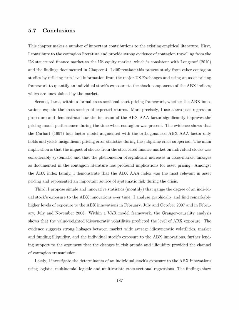
5.7 Conclusions
This chapter makes a number of important contributions to the existing empirical literature. First,
I contribute to the contagion literature and provide strong evidence of contagion travelling from the
US structured finance market to the US equity market, which is consistent with Longstaff (2010)
and the findings documented in Chapter 4. I differentiate this present study from other contagion
studies by utilising firm-level information from the major US Exchanges and using an asset pricing
framework to quantify an individual stock’s exposure to the shock components of the ABX indices,
which are unexplained by the market.
Second, I test, within a formal cross-sectional asset pricing framework, whether the ABX inno-
vations explain the cross-section of expected returns. More precisely, I use a two-pass regression
procedure and demonstrate how the inclusion of the ABX AAA factor significantly improves the
pricing model performance during the time when contagion was present. The evidence shows that
the Carhart (1997) four-factor model augmented with the orthogonalised ABX AAA factor only
holds and yields insignificant pricing error statistics during the subprime crisis subperiod. The main
implication is that the impact of shocks from the structured finance market on individual stocks was
considerably systematic and that the phenomenon of significant increases in cross-market linkages
as documented in the contagion literature has profound implications for asset pricing. Amongst
the ABX index family, I demonstrate that the ABX AAA index was the most relevant in asset
pricing and represented an important source of systematic risk during the crisis.
Third, I propose simple and innovative statistics (monthly) that gauge the degree of an individ-
ual stock’s exposure to the ABX innovations over time. I analyse graphically and find remarkably
higher levels of exposure to the ABX innovations in February, July and October 2007 and in Febru-
ary, July and November 2008. Within a VAR model framework, the Granger-causality analysis
shows that the value-weighted idiosyncratic volatilities predicted the level of ABX exposure. The
evidence suggests strong linkages between market wide average idiosyncratic volatilities, market
and funding illiquidity, and the individual stock’s exposure to the ABX innovations, further lend-
ing support to the argument that the changes in risk premia and illiquidity provided the channel
of contagion transmission.
Lastly, I investigate the determinants of an individual stock’s exposure to the ABX innovations
using logistic, multinomial logistic and multivariate cross-sectional regressions. The findings show
187

that higher idiosyncratic volatilities and lower standard deviations are associated with higher (and
also higher likelihood of having significant) ABX factor loadings, more prominently in the ABX
AAA and AA models. I also find positive relations between the market betas and the ABX factor
loadings. Nonetheless, I find little evidence that the firm-specific fundamental variables explain the
individual stock’s exposure to the ABX innovations.
188
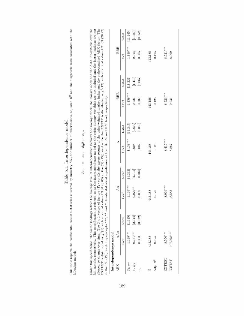
Table
5.1:Interdep
endence
model
This
table
reportsth
eco
efficien
ts,robust
t-statisticsclustered
byindustry
SIC
,th
enumber
ofobservations,
adjusted
R2andth
ediagnostic
testsassociatedwithth
efollowingmodel:
Ri,t
=αi,t+
β′ 0F
t+
ε i,t.
Under
this
specifica
tion,th
efactorloadingsreflectth
eaveragelevel
ofinterd
epen
den
cebetweenth
eaveragestock
,th
emarket
index
andth
eABX
innovationsover
the
fullsample,resp
ectively.
This
specifica
tionis
referred
toasth
einterd
epen
den
cemodel
asth
ecrisis
dummyvariablesare
notincluded
andth
efactorloadingsare
not
allowed
toch
angeover
time.
The2×
1vectoroffactors
(Ft)en
tailsth
eex
cess
retu
rnsofth
evalue-weightedmarket
index
andth
eorthogonalisedABX
factor.
The
EXTEST
isdistributedasχ2(1)withacriticalvalueof3.84(6.63)atth
e5%
(1%)level
whileth
eIC
STAT
isdistributedasχ2(12)withacriticalvalueof21.03(26.22)
atth
e5%
(1%)level.Superscripts
***,**and*den
ote
statisticalsignifica
nce
atth
e1%,5%
and10%
level,resp
ectively.
Inte
rdependencem
odel
ABX
AAA
AA
ABBB
BBB-
Coef.
t-stat
Coef.
t-stat
Coef.
t-stat
Coef.
t-stat
Coef.
t-stat
βM
KT
1.139∗∗
∗[11.345]
1.139∗∗
∗[11.292]
1.138∗∗
∗[11.247]
1.138∗∗
∗[11.227]
1.138∗∗
∗[11.245]
βABX
0.151∗∗
∗[2.944]
0.029∗∗
[2.105]
0.008
[0.619]
0.021
[1.410]
0.015
[1.087]
α0
0.003
[0.032]
0.002
[0.018]
0.002
[0.018]
0.007
[0.067]
0.005
[0.052]
N443,188
443,188
443,188
443,188
443,188
Adj.
R2
0.125
0.125
0.125
0.125
0.125
EXTEST
8.556∗∗
∗8.069∗∗
∗8.415∗∗
∗8.523∗∗
∗8.521∗∗
∗
ICSTAT
107.978∗∗
∗8.583
8.887
9.031
8.999
189
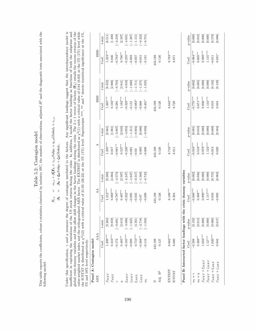
Table
5.2:Contagionmodel
This
table
reportsth
eco
efficien
ts,robust
t-statisticsclustered
byindustry
SIC
,th
enumber
ofobservations,
adjusted
R2andth
ediagnostic
testsassociatedwithth
efollowingmodel:
Ri,t
=αi,t+
β′ tF
t+
γi,0Subp
t+
ηi,0Globa
l t+
ε i,t,
βt
=β0+
ξ0Subp
t+
ζ0Globa
l t.
Under
this
specifica
tion,γ
and
ηmea
sure
thedeg
reeofco
ntagion
unrelated
toth
efactors.
Any
significa
ntloadingssu
ggestth
atth
einterd
epen
den
cemodel
isinsu
fficien
tin
captu
ringth
evariationsofth
eUS
stock
retu
rnsduringth
ecrisis.
Inaddition,Imodel
thefactorloadingsasfunctionsofboth
thesu
bprimeand
globalcrisis
dummyvariablesandthusallow
shiftch
anges
inth
efactorloadingsduringth
ecrisis.The2×
1vectoroffactors
(Ft)en
tailsth
eex
cess
retu
rnsofth
evalue-weightedmarket
index
andth
eorthogonalisedABX
factor.
TheEXTEST
isdistributedasχ2(1)withacriticalvalueof3.84(6.63)atth
e5%
(1%)level
while
theIC
STAT
isdistributedasχ2(12)withacriticalvalueof21.03(26.22)atth
e5%
(1%)level.Superscripts
***,**and*den
ote
statisticalsignifica
nce
atth
e1%,
5%
and10%
level
resp
ectively.
PanelA:Conta
gion
model
ABX
AAA
AA
ABBB
BBB-
Coef.
t-stat
Coef.
t-stat
Coef.
t-stat
Coef.
t-stat
Coef.
t-stat
βM
KT
1.209∗∗
∗[9.263]
1.212∗∗
∗[9.260]
1.205∗∗
∗[8.861]
1.265∗∗
∗[8.352]
1.224∗∗
∗[8.511]
βABX
0.310∗∗
∗[9.859]
0.068∗∗
∗[4.004]
0.017
[1.061]
0.102∗∗
∗[2.806]
0.046
[1.400]
γ−0.172
[−0.691]
−0.787∗∗
[−2.573]
−0.901∗∗
[−2.867]
−0.285
[−0.703]
−0.783∗∗
[−2.259]
η0.485∗∗
[2.619]
0.407∗∗
[2.597]
0.527∗∗
[2.623]
1.162∗∗
∗[3.841]
0.786∗∗
[2.597]
ξ MK
T−0.185∗∗
∗[−
3.086]
−0.222∗∗
[−2.247]
−0.226∗∗
∗[−
4.052]
−0.329∗∗
∗[−
4.943]
−0.235∗∗
∗[−
4.031]
ζ MK
T−0.089
[−1.625]
−0.095
[−1.647]
−0.081
[−1.311]
−0.131
[−1.660]
−0.093
[−1.387]
ξ ABX
0.710∗∗
∗[4.561]
−0.035
[−0.317]
−0.03
[−0.684]
−0.083∗
[−1.711]
−0.057
[−1.151]
ζ ABX
−0.268∗∗
[−2.718]
−0.07
[−1.569]
0.003
[0.086]
−0.068
[−1.275]
−0.015
[−0.322]
α0
−0.116
[−1.058]
−0.099
[−0.743]
−0.009
[−0.056]
−0.491∗
[−1.825]
−0.181
[−0.751]
N443,188
443,188
443,188
443,188
443,188
Adj.
R2
0.127
0.126
0.126
0.126
0.126
EXTEST
8.662∗∗
∗8.106∗∗
∗8.716∗∗
∗8.643∗∗
∗8.783∗∗
∗
ICSTAT
8.680
8.384
8.811
8.728
8.871
PanelB:In
teracte
dfacto
rloadin
gswith
thecrisis
dum
my
variables
Coef.
p-value
Coef.
p-value
Coef.
p-value
Coef.
p-value
Coef.
p-value
α0+
γ−0.288
[0.192]
−0.886∗∗
∗[0.002]
−0.910∗∗
∗[0.001]
−0.776∗∗
∗[0.002]
−0.964∗∗
∗[0.000]
α0+
η0.369∗∗
[0.013]
0.308∗∗
[0.036]
0.518∗∗
∗[0.010]
0.671∗∗
∗[0.005]
0.605∗∗
[0.010]
βM
KT+
ξ MK
T1.024∗∗
∗[0.000]
0.990∗∗
∗[0.000]
0.979∗∗
∗[0.000]
0.936∗∗
∗[0.000]
0.989∗∗
∗[0.000]
βM
KT+
ζ MK
T1.12∗∗
∗[0.000]
1.117∗∗
∗[0.000]
1.124∗∗
∗[0.000]
1.134∗∗
∗[0.000]
1.131∗∗
∗[0.000]
βABX
+ξ A
BX
1.020∗∗
∗[0.000]
0.033
[0.755]
−0.013
[0.669]
0.019
[0.192]
−0.011
[0.579]
βABX
+ζ A
BX
0.042
[0.617]
−0.002
[0.963]
0.020
[0.384]
0.034
[0.129]
0.031∗
[0.086]
190
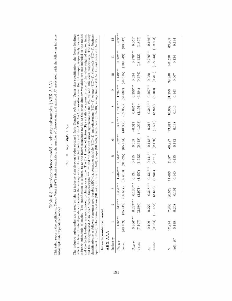
Tab
le5.3:Interdep
endence
model
-industry
subsamples(A
BX
AAA)
This
table
reportsth
eco
efficien
ts,New
ey-W
est(1987)robust
t-statistics,
thenumber
ofobservationsandadjusted
R2associatedwithth
efollowingindustry
subsample
interd
epen
den
cemodel:
Ri,t
=αi,t+
β′ 0F
t+
ε i,t.
Theindustry
subsamplesare
based
on
the12-industry
classifica
tion
codes
obtained
from
French
’sweb
site.
Under
this
specifica
tion,th
efactorloadings
reflectth
elevel
ofinterd
epen
den
cebetweenth
eaveragestock
,th
emarket
index
andth
eABX
AAA
innovationsover
thefullsample,resp
ectively,
forea
chindustry
subsample
ofstock
s.This
specifica
tion
isreferred
toasth
einterd
epen
den
cemodel
asth
ecrisis
dummyvariablesare
notincluded
inth
emodel
andth
efactorloadingsare
notallowed
toch
angeover
time.
The2×
1vectoroffactors
(Ft)en
tailsth
eex
cess
retu
rnsofth
evalue-weightedmarket
index
andth
eorthogonalisedABX
AAA
factor.
Superscripts
***,**and*den
ote
statisticalsignifica
nce
atth
e1%,5%
and10%
level,resp
ectively.
Theindustry
classifica
tionis
asfollows:
consu
mer
non-durable
(SIC
=1),
consu
mer
durable
(SIC
=2),
manufacturing(S
IC=3),
energy(S
IC=4),
chem
icals
(SIC
=5),
business
equipmen
t(S
IC=6),
teleco
mmunication(S
IC=7),
utilities
(SIC
=8),
shops(S
IC=9),
hea
lthca
re(S
IC=10),
money
finance
(SIC
=11),
andoth
er(S
IC=12).
Inte
rdependencem
odel
ABX
AAA
Industry
12
34
56
78
910
11
12
βM
KT
1.136∗∗
∗1.617∗∗
∗1.454∗∗
∗1.502∗∗
∗1.334∗∗
∗1.282∗∗
∗1.300∗∗
∗0.705∗∗
∗1.287∗∗
∗1.149∗∗
∗0.862∗∗
∗1.239∗∗
∗
t-stat
(40.409)
(35.419)
(68.517)
(39.610)
(31.925)
(85.434)
(40.386)
(32.353)
(54.887)
(44.515)
(109.849)
(83.312)
βABX
0.366∗∗
∗0.237∗∗
∗0.130∗∗
∗0.134
0.115
0.009
−0.071
0.085∗∗
0.256∗∗
∗0.024
0.270∗∗
∗0.051∗
t-stat
(7.107)
(2.680)
(2.971)
(1.457)
(1.552)
(0.318)
(−1.063)
(2.151)
(6.384)
(0.474)
(18.422)
(1.857)
α0
0.109
−0.279
0.318∗∗
∗0.431∗∗
∗0.441∗∗
0.148∗∗
0.217
0.343∗∗
∗0.287∗∗
∗0.080
−0.276∗∗
∗−0.166∗∗
t-stat
(0.964)
(−1.483)
(3.643)
(2.934)
(2.371)
(2.130)
(1.500)
(3.929)
(3.100)
(0.701)
(−8.943)
(−2.503)
N17,824
7,840
30,579
17,686
7,687
60,887
13,871
10,908
31,356
38,940
141,520
63,805
Adj.
R2
0.139
0.208
0.197
0.140
0.155
0.132
0.138
0.146
0.143
0.067
0.134
0.134
191

Tab
le5.4:Interdep
endence
model
-industry
subsamples(A
BX
AA)
This
table
reportsth
eco
efficien
ts,New
ey-W
est(1987)robust
t-statistics,
thenumber
ofobservationsandadjusted
R2associatedwithth
efollowingindustry
subsample
interd
epen
den
cemodel:
Ri,t
=αi,t+
β′ 0F
t+
ε i,t.
Theindustry
subsample
isbasedonth
e12-industry
classifica
tionco
des
obtained
from
French
’sweb
site.Under
this
specifica
tion,th
efactorloadingsreflect
thelevel
ofinterd
epen
den
cebetween
theaveragestock
,th
emarket
index
and
theABX
AA
innovationsover
thefull
sample,resp
ectively,
forea
chindustry
subsample
ofstock
s.This
specifica
tion
isreferred
toasth
einterd
epen
den
cemodel
asth
ecrisis
dummy
variablesare
notincluded
inth
emodel
and
the
factorloadingsare
notallowed
toch
angeover
time.
The2×
1vectoroffactors
(Ft)en
tailsth
eex
cess
retu
rnsofth
evalue-weighted
market
index
and
the
orthogonalisedABX
AA
factor.
Superscripts
***,**and*den
ote
statisticalsignifica
nce
atth
e1%,5%
and10%
level
resp
ectively.
Theindustry
classifica
tion
isasfollows:
consu
mer
non-durable
(SIC
=1),
consu
mer
durable
(SIC
=2),
manufacturing(S
IC=3),
energy(S
IC=4),
chem
icals
(SIC
=5),
businesseq
uipmen
t(S
IC=6),
teleco
mmunication(S
IC=7),
utilities
(SIC
=8),
shops(S
IC=9),
hea
lthca
re(S
IC=10),
money
finance
(SIC
=11),
andoth
er(S
IC=12).
Inte
rdependencem
odel
ABX
AA
Industry
12
34
56
78
910
11
12
βM
KT
1.135∗∗
∗1.618∗∗
∗1.454∗∗
∗1.502∗∗
∗1.335∗∗
∗1.282∗∗
∗1.299∗∗
∗0.705∗∗
∗1.287∗∗
∗1.149∗∗
∗0.860∗∗
∗1.239∗∗
∗
t-stat
(40.247)
(35.307)
(68.461)
(39.621)
(31.875)
(85.414)
(40.281)
(32.343)
(54.749)
(44.526)
(109.310)
(83.456)
βABX
0.083∗∗
∗0.020
−0.015
0.058
−0.001
−0.007
−0.003
0.031∗∗
−0.001
0.016
0.066∗∗
∗0.018∗∗
t-stat
(5.364)
(0.668)
(−0.948)
(1.689)
(−0.056)
(−0.782)
(−0.141)
(2.542)
(−0.107)
(0.841)
(13.252)
(2.022)
α0
0.106
−0.284
0.314∗∗
∗0.433∗∗
∗0.438∗∗
0.147∗∗
0.219
0.343∗∗
∗0.281∗∗
∗0.080
−0.278∗∗
∗−0.165∗∗
t-stat
(0.935)
(−1.512)
(3.595)
(2.953)
(2.351)
(2.120)
(1.514)
(3.928)
(3.026)
(0.705)
(−8.978)
(−2.489)
N17,824
7,840
30,579
17,686
7,687
60,887
13,871
10,908
31,356
38,940
141,520
63,805
Adj.
R2
0.136
0.207
0.197
0.141
0.155
0.132
0.138
0.146
0.141
0.067
0.132
0.134
192
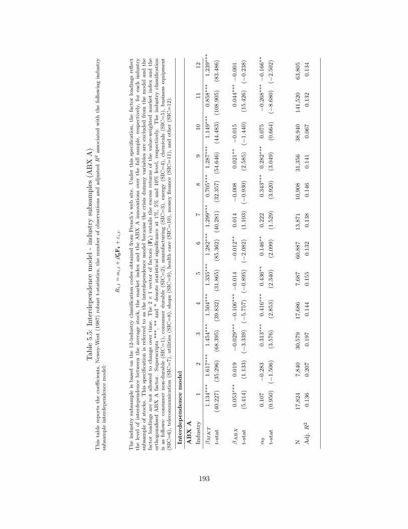
Tab
le5.5:Interdep
endence
model
-industry
subsamples(A
BX
A)
This
table
reportsth
eco
efficien
ts,New
ey-W
est(1987)robust
t-statistics,
thenumber
ofobservationsandadjusted
R2associatedwithth
efollowingindustry
subsample
interd
epen
den
cemodel:
Ri,t=
αi,t+
β′ 0F
t+
ε i,t.
Theindustry
subsample
isbasedonth
e12-industry
classifica
tionco
des
obtained
from
French
’sweb
site.Under
this
specifica
tion,th
efactorloadingsreflect
thelevel
ofinterd
epen
den
cebetween
theaveragestock
,th
emarket
index
and
theABX
Ainnovationsover
thefull
sample,resp
ectively,
forea
chindustry
subsample
ofstock
s.This
specifica
tionis
referred
toasth
einterd
epen
den
cemodel
because
thecrisis
dummyvariablesare
excluded
from
themodel
andth
efactorloadingsare
notallowed
toch
angeover
time.
The2×
1vectoroffactors
(Ft)en
tailsth
eex
cess
retu
rnsofth
evalue-weighted
market
index
and
the
orthogonalised
ABX
Afactor.
Superscripts
***,**and
*den
ote
statisticalsignifica
nce
at1%,5%
and
10%
level,resp
ectively.
Theindustry
classifica
tion
isasfollows:
consu
mer
non-durable
(SIC
=1),
consu
mer
durable
(SIC
=2),
manufacturing(S
IC=3),
energy(S
IC=4),
chem
icals
(SIC
=5),
businesseq
uipmen
t(S
IC=6),
teleco
mmunication(S
IC=7),
utilities
(SIC
=8),
shops(S
IC=9),
hea
lthca
re(S
IC=10),
money
finance
(SIC
=11),
andoth
er(S
IC=12).
Inte
rdependencem
odel
ABX
A
Industry
12
34
56
78
910
11
12
βM
KT
1.134∗∗
∗1.617∗∗
∗1.454∗∗
∗1.504∗∗
∗1.335∗∗
∗1.282∗∗
∗1.299∗∗
∗0.705∗∗
∗1.287∗∗
∗1.149∗∗
∗0.858∗∗
∗1.239∗∗
∗
t-stat
(40.227)
(35.296)
(68.395)
(39.832)
(31.865)
(85.362)
(40.281)
(32.357)
(54.646)
(44.483)
(108.905)
(83.486)
βABX
0.053∗∗
∗0.019
−0.029∗∗
∗−0.106∗∗
∗−0.014
−0.012∗∗
0.014
−0.008
0.021∗∗
−0.015
0.044∗∗
∗−0.001
t-stat
(5.414)
(1.133)
(−3.339)
(−5.757)
(−0.895)
(−2.082)
(1.103)
(−0.930)
(2.585)
(−1.440)
(15.426)
(−0.238)
α0
0.107
−0.283
0.313∗∗
∗0.416∗∗
∗0.436∗∗
0.146∗∗
0.222
0.343∗∗
∗0.282∗∗
∗0.075
−0.268∗∗
∗−0.166∗∗
t-stat
(0.950)
(−1.506)
(3.576)
(2.853)
(2.340)
(2.099)
(1.529)
(3.920)
(3.049)
(0.664)
(−8.680)
(−2.502)
N17,824
7,840
30,579
17,686
7,687
60,887
13,871
10,908
31,356
38,940
141,520
63,805
Adj.
R2
0.136
0.207
0.197
0.144
0.155
0.132
0.138
0.146
0.141
0.067
0.132
0.134
193

Tab
le5.6:Interdep
endence
model
-industry
subsamples(A
BX
BBB)
This
table
reportsth
eco
efficien
ts,New
ey-W
est(1987)robust
t-statistics,
thenumber
ofobservationsandadjusted
R2associatedwithth
efollowingindustry
subsample
interd
epen
den
cemodel:
Ri,t=
αi,t+
β′ 0F
t+
ε i,t
Theindustry
subsample
isbasedonth
e12-industry
classifica
tionco
des
obtained
from
French
’sweb
site.Under
this
specifica
tion,th
efactorloadingsreflect
thelevel
ofinterd
epen
den
cebetweenth
eaveragestock
,th
emarket
index
andth
eABX
BBB
innovationsover
thefullsample,resp
ectively,
forea
chindustry
subsample
ofstock
s.This
specifica
tionis
referred
toasth
einterd
epen
den
cemodel
because
thecrisis
dummyvariablesare
notincluded
inth
emodel
andth
efactorloadingsare
notallowed
toch
angeover
time.
The2×
1vectoroffactors
(Ft)en
tailsth
eex
cess
retu
rnsofth
evalue-weighted
market
index
and
the
orthogonalisedABX
BBB
factor.
Superscripts
***,**and*den
ote
statisticalsignifica
nce
atth
e1%,5%
and10%
level,resp
ectively.
Theindustry
classifica
tion
isasfollows:
consu
mer
non-durable
(SIC
=1),
consu
mer
durable
(SIC
=2),
manufacturing(S
IC=3),
energy(S
IC=4),
chem
icals
(SIC
=5),
businesseq
uipmen
t(S
IC=6),
teleco
mmunication(S
IC=7),
utilities
(SIC
=8),
shops(S
IC=9),
hea
lthca
re(S
IC=10),
money
finance
(SIC
=11),
andoth
er(S
IC=12).
Inte
rdependencem
odel
ABX
BBB
Industry
12
34
56
78
910
11
12
βM
KT
1.134∗∗
∗1.617∗∗
∗1.454∗∗
∗1.504∗∗
∗1.335∗∗
∗1.282∗∗
∗1.298∗∗
∗0.705∗∗
∗1.285∗∗
∗1.148∗∗
∗0.857∗∗
∗1.239∗∗
∗
t-stat
(40.232)
(35.304)
(68.359)
(39.768)
(31.846)
(85.370)
(40.285)
(32.358)
(54.662)
(44.451)
(108.878)
(83.464)
βABX
0.071∗∗
∗0.018
−0.020∗∗
−0.118∗∗
∗0.001
0.005
0.032∗∗
−0.004
0.055∗∗
∗0.018∗
0.055∗∗
∗−0.009
t-stat
(6.597)
(1.115)
(−2.330)
(−7.159)
(0.079)
(0.776)
(2.204)
(−0.373)
(6.673)
(1.710)
(19.748)
(−1.537)
α0
0.114
−0.281
0.312∗∗
∗0.408∗∗
∗0.438∗∗
0.149∗∗
0.231
0.343∗∗
∗0.294∗∗
0.087
−0.252∗∗
∗−0.165∗∗
t-stat
(1.008)
(−1.497)
(3.571)
(2.801)
(2.351)
(2.150)
(1.599)
(3.921)
(3.188)
(0.774)
(−8.150)
(−2.484)
N17,824
7,840
30,579
17,686
7,687
60,887
13,871
10,908
31,356
38,940
141,520
63,805
Adj.
R2
0.136
0.207
0.197
0.144
0.155
0.132
0.138
0.146
0.142
0.067
0.133
0.134
194
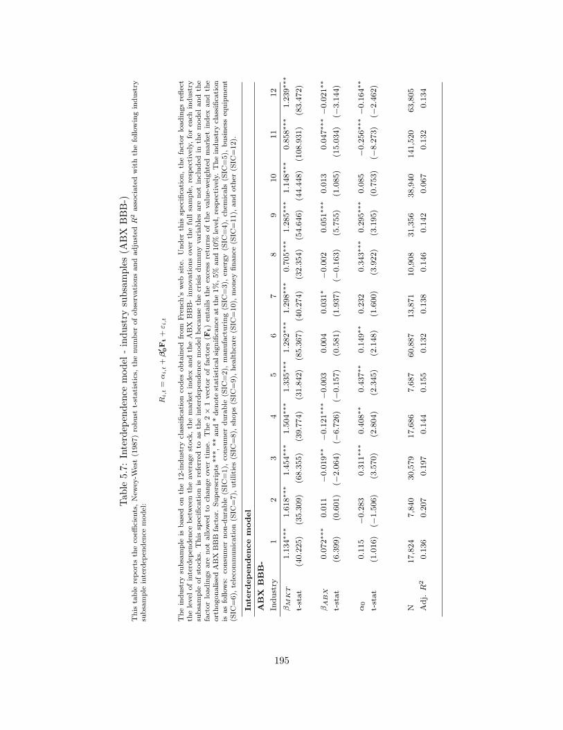
Tab
le5.7:Interdep
endence
model
-industry
subsamples(A
BX
BBB-)
This
table
reportsth
eco
efficien
ts,New
ey-W
est(1987)robust
t-statistics,
thenumber
ofobservationsandadjusted
R2associatedwithth
efollowingindustry
subsample
interd
epen
den
cemodel:
Ri,t=
αi,t+
β′ 0F
t+
ε i,t
Theindustry
subsample
isbasedonth
e12-industry
classifica
tionco
des
obtained
from
French
’sweb
site.Under
this
specifica
tion,th
efactorloadingsreflect
thelevel
ofinterd
epen
den
cebetweenth
eaveragestock
,th
emarket
index
andth
eABX
BBB-innovationsover
thefullsample,resp
ectively,
forea
chindustry
subsample
ofstock
s.This
specifica
tionis
referred
toasth
einterd
epen
den
cemodel
because
thecrisis
dummyvariablesare
notincluded
inth
emodel
andth
efactorloadingsare
notallowed
toch
angeover
time.
The2×
1vectoroffactors
(Ft)en
tailsth
eex
cess
retu
rnsofth
evalue-weighted
market
index
and
the
orthogonalisedABX
BBB
factor.
Superscripts
***,**and*den
ote
statisticalsignifica
nce
atth
e1%,5%
and10%
level,resp
ectively.
Theindustry
classifica
tion
isasfollows:
consu
mer
non-durable
(SIC
=1),
consu
mer
durable
(SIC
=2),
manufacturing(S
IC=3),
energy(S
IC=4),
chem
icals
(SIC
=5),
businesseq
uipmen
t(S
IC=6),
teleco
mmunication(S
IC=7),
utilities
(SIC
=8),
shops(S
IC=9),
hea
lthca
re(S
IC=10),
money
finance
(SIC
=11),
andoth
er(S
IC=12).
Inte
rdependencem
odel
ABX
BBB-
Industry
12
34
56
78
910
11
12
βM
KT
1.134∗∗
∗1.618∗∗
∗1.454∗∗
∗1.504∗∗
∗1.335∗∗
∗1.282∗∗
∗1.298∗∗
∗0.705∗∗
∗1.285∗∗
∗1.148∗∗
∗0.858∗∗
∗1.239∗∗
∗
t-stat
(40.225)
(35.309)
(68.355)
(39.774)
(31.842)
(85.367)
(40.274)
(32.354)
(54.646)
(44.448)
(108.931)
(83.472)
βABX
0.072∗∗
∗0.011
−0.019∗∗
−0.121∗∗
∗−0.003
0.004
0.031∗
−0.002
0.051∗∗
∗0.013
0.047∗∗
∗−0.021∗∗
t-stat
(6.399)
(0.601)
(−2.064)
(−6.726)
(−0.157)
(0.581)
(1.937)
(−0.163)
(5.755)
(1.085)
(15.034)
(−3.144)
α0
0.115
−0.283
0.311∗∗
∗0.408∗∗
0.437∗∗
0.149∗∗
0.232
0.343∗∗
∗0.295∗∗
∗0.085
−0.256∗∗
∗−0.164∗∗
t-stat
(1.016)
(−1.506)
(3.570)
(2.804)
(2.345)
(2.148)
(1.600)
(3.922)
(3.195)
(0.753)
(−8.273)
(−2.462)
N17,824
7,840
30,579
17,686
7,687
60,887
13,871
10,908
31,356
38,940
141,520
63,805
Adj.
R2
0.136
0.207
0.197
0.144
0.155
0.132
0.138
0.146
0.142
0.067
0.132
0.134
195

Tab
le5.8:Contagionmodel
-industry
subsample
(ABX
AAA)
This
table
reportsth
eco
efficien
ts,robust
t-statistics,
thenumber
ofobservationsandadjusted
R2associatedwithth
efollowingindustry
subsample
contagionmodel:
Ri,t
=αi,t+
β′ tF
t+
γi,0Subp
t+
ηi,0Globa
l t+
ε i,t,
βt
=β0+
ξ0Subp
t+
ζ0Globa
l t.
Under
this
specifica
tion,γandηmea
sure
thedeg
reeofco
ntagionunrelatedto
thefactors
andth
atanysignifica
ntloadingssu
ggestth
at
theinterd
epen
den
cemodel
isinsu
fficien
tin
captu
ringth
evariationsofstock
retu
rnsin
individualindustry
sectors.In
addition,Imodel
thefactorloadingsasfunctionsofboth
thesu
bprimeandglobalcrisis
dummyvariablesandthusallow
shiftch
anges
inth
efactorloadings
duringth
ecrisis.The2×
1vectoroffactors
(Ft)en
tailsth
eex
cess
retu
rnsofth
evalue-weightedmarket
index
andth
eorthogonalised
ABX
AAA
innovations.
Superscripts
***,**and*den
ote
statisticalsignifica
nce
atth
e1%,5%
and10%
level
resp
ectively.
Theindustry
classifica
tionis
asfollows:
consu
mer
non-durable
(SIC
=1),
consu
mer
durable
(SIC
=2),
manufacturing(S
IC=3),
energy(S
IC=4),
chem
icals
(SIC
=5),businesseq
uipmen
t(S
IC=6),teleco
mmunication(S
IC=7),utilities
(SIC
=8),sh
ops(S
IC=9),hea
lthca
re(S
IC=10),money
finance
(SIC
=11),
andoth
er(S
IC=12).
PanelA
:Contagio
nM
odel
ABX
AA
A
Industry
12
34
56
78
910
11
12
βM
KT
1.224∗∗∗
1.730∗∗∗
1.551∗∗∗
1.652∗∗∗
1.507∗∗∗
1.396∗∗∗
1.326∗∗∗
0.648∗∗∗
1.387∗∗∗
1.287∗∗∗
0.832∗∗∗
1.357∗∗∗
t-stat
(30.305)
(26.286)
(56.825)
(45.337)
(25.726)
(66.486)
(31.264)
(24.756)
(36.256)
(34.784)
(75.914)
(67.385)
βA
BX
0.594∗∗∗
0.674∗∗∗
0.322∗∗∗
0.548∗∗∗
0.248∗∗
0.297∗∗∗
0.035
0.165∗∗∗
0.476∗∗∗
0.225∗∗∗
0.249∗∗∗
0.309∗∗∗
t-stat
(6.806)
(4.586)
(5.930)
(7.672)
(2.263)
(6.631)
(0.333)
(3.413)
(7.357)
(3.328)
(11.607)
(7.871)
γ0.150
0.317
1.046∗∗∗
1.007∗∗
1.356∗∗
0.307
−0.465
−0.586∗∗
−0.990∗∗∗
−0.731∗∗
−0.716∗∗∗
0.241
t-stat
(0.484)
(0.683)
(4.304)
(3.252)
(2.495)
(1.514)
(−1.216)
(−2.101)
(−3.879)
(−2.399)
(−10.580)
(1.241)
η−0.462
−0.024
0.518
1.501∗
−0.116
0.411∗
−1.577∗∗∗
−0.839∗∗∗
1.173∗∗∗
1.231∗∗∗
0.174
1.069∗∗∗
t-stat
(−1.220)
(−0.038)
(1.461)
(1.931)
(−0.204)
(1.810)
(−3.398)
(−2.972)
(3.818)
(3.149)
(1.639)
(4.741)
ξM
KT
−0.210∗∗
−0.437∗∗
−0.490∗∗∗
−0.329∗∗∗
−0.560∗∗∗
−0.354∗∗∗
−0.002
−0.002
−0.314∗∗∗
−0.141
−0.013
−0.042
t-stat
(−2.415)
(−3.043)
(−6.897)
(−4.098)
(−4.208)
(−6.840)
(−0.018)
(−0.035)
(−3.942)
(−1.644)
(−0.670)
(−0.765)
ζM
KT
−0.184∗∗∗
−0.178
−0.112∗∗
−0.189
−0.296∗∗∗
−0.163∗∗∗
−0.144∗
0.072
−0.088
−0.187∗∗∗
0.083∗∗∗
−0.182∗∗∗
t-stat
(−2.810)
(−1.629)
(−2.011)
(−1.603)
(−3.164)
(−4.778)
(−1.955)
(1.489)
(−1.629)
(−3.013)
(4.616)
(−5.245)
ξA
BX
1.353∗∗∗
1.142∗∗
1.033∗∗∗
−0.498
1.724∗∗∗
0.736∗∗∗
0.970∗∗
−0.483
1.234∗∗∗
0.238
0.961∗∗∗
−0.000
t-stat
(3.584)
(2.055)
(3.611)
(−1.365)
(2.960)
(3.071)
(2.042)
(−1.461)
(4.092)
(0.571)
(11.923)
(−0.002)
ζA
BX
−0.429∗∗∗
−0.748∗∗∗
−0.311∗∗∗
−0.609∗∗∗
−0.245
−0.477∗∗∗
−0.264∗
−0.174∗∗
−0.376∗∗∗
−0.303∗∗
0.002
−0.387∗∗∗
t-stat
(−3.916)
(−4.101)
(−3.854)
(−4.174)
(−1.627)
(−8.174)
(−1.892)
(−2.262)
(−4.509)
(−3.148)
(0.065)
(−6.996)
α0
0.085
−0.509∗∗
−0.013
−0.427∗∗∗
0.123
−0.142
0.587∗∗∗
0.598∗∗∗
0.220∗∗
−0.256∗
0.015
−0.674∗∗∗
t-stat
(0.638)
(−2.272)
(−0.122)
(−3.001)
(0.502)
(−1.585)
(2.965)
(5.995)
(2.039)
(−1.938)
(0.389)
(−8.593)
N17,824
7,840
30,579
17,686
7,687
60,887
13,871
10,908
31,356
38,940
141,520
63,805
Adj.
R2
0.142
0.213
0.199
0.143
0.158
0.135
0.139
0.148
0.148
0.069
0.136
0.136
PanelB:Interacted
factor
loadin
gs
α0+
γ0.235
−0.192
1.033∗∗∗
0.580∗∗
1.479∗∗∗
0.165
0.122
0.012
−0.770∗∗∗
−0.987∗∗∗
−0.701∗∗∗
−0.433∗∗
α0+
η−0.377
−0.533
0.505
1.074
0.007
0.269
−0.990∗∗
−0.241
1.393∗∗∗
0.975∗∗∗
0.189∗
0.395∗
βM
KT
+ξM
KT
1.014∗∗∗
1.293∗∗∗
1.061∗∗∗
1.323∗∗∗
0.947∗∗∗
1.042∗∗∗
1.324∗∗∗
0.646∗∗∗
1.073∗∗∗
1.146∗∗∗
0.819∗∗∗
1.315∗∗∗
βM
KT
+ζM
KT
1.040∗∗∗
1.552∗∗∗
1.439∗∗∗
1.463∗∗∗
1.211∗∗∗
1.233∗∗∗
1.182∗∗∗
0.720∗∗∗
1.299∗∗∗
1.100∗∗∗
0.915∗∗∗
1.175∗∗∗
βA
BX
+ξA
BX
1.947∗∗∗
1.816∗∗∗
1.355∗∗∗
0.050
1.972∗∗∗
1.033∗∗∗
1.005∗∗
−0.318
1.710∗∗∗
0.463
1.210∗∗∗
0.309
βA
BX
+ζA
BX
0.165∗∗
−0.074
0.011
−0.061
0.003
−0.180∗∗∗
−0.229∗∗
−0.009
0.100∗
−0.078
0.251∗∗∗
−0.078∗∗
196
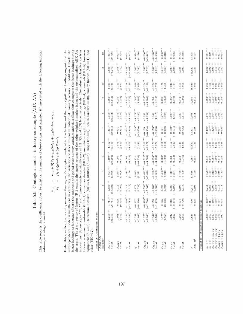
Tab
le5.9:Contagionmodel
-industry
subsample
(ABX
AA)
This
table
reportsth
eco
efficien
ts,robust
t-statistics,
thenumber
ofobservationsandadjusted
R2associatedwithth
efollowingindustry
subsample
contagionmodel:
Ri,t
=αi,t+
β′ tF
t+
γi,0Subp
t+
ηi,0Globa
l t+
ε i,t,
βt
=β0+
ξ0Subp
t+
ζ0Globa
l t.
Under
this
specifica
tion,γandηmea
sure
thedeg
reeofco
ntagionunrelatedto
thefactors
andth
atanysignifica
ntloadingssu
ggestth
atth
einterd
epen
den
cemodel
isinsu
fficien
tin
captu
ringth
evariationsofstock
retu
rnsin
individualindustry
sectors.In
addition,Imodel
the
factorloadingsasfunctionsofboth
thesu
bprimeandglobalcrisisdummyvariablesandthusallow
shiftch
anges
inth
efactorloadingsduring
thecrisis.The2×
1vectoroffactors
(Ft)en
tailsth
eex
cess
retu
rnsofth
evalue-weightedmarket
index
andth
eorthogonalisedABX
AA
innovations.
Superscripts
***,**and*den
ote
statisticalsignifica
nce
at1%,5%
and10%
level
resp
ectively.
Theindustry
classifica
tionis
as
follows:
consu
mer
non-durable
(SIC
=1),co
nsu
mer
durable
(SIC
=2),manufacturing(S
IC=3),en
ergy(S
IC=4),ch
emicals(S
IC=5),business
equipmen
t(S
IC=6),
teleco
mmunication(S
IC=7),
utilities
(SIC
=8),
shops(S
IC=9),
hea
lthca
re(S
IC=10),
money
finance
(SIC
=11),
and
oth
er(S
IC=12).
PanelA
:Contagio
nM
odel
ABX
AA
Industry
12
34
56
78
910
11
12
βM
KT
1.215∗∗∗
1.711∗∗∗
1.535∗∗∗
1.694∗∗∗
1.499∗∗∗
1.402∗∗∗
1.331∗∗∗
0.658∗∗∗
1.361∗∗∗
1.317∗∗∗
0.834∗∗∗
1.361∗∗∗
t-stat
(31.153)
(26.781)
(57.721)
(47.076)
(26.294)
(67.763)
(32.061)
(25.751)
(38.144)
(33.735)
(78.277)
(69.746)
βA
BX
0.068∗∗∗
0.022
−0.012
0.274∗∗∗
0.005
0.071∗∗∗
0.024
0.074∗∗∗
−0.036∗
0.153∗∗∗
0.051∗∗∗
0.097∗∗∗
t-stat
(3.243)
(0.575)
(−0.769)
(12.006)
(0.171)
(5.850)
(0.831)
(5.437)
(−1.923)
(5.617)
(7.740)
(8.595)
γ−1.154∗∗∗
−1.069∗∗∗
0.043
1.284∗∗∗
0.094
−0.319∗∗
−1.024∗∗∗
−0.342∗
−2.336∗∗∗
−0.758∗∗∗
−1.421∗∗∗
0.054
t-stat
(−4.584)
(−2.713)
(0.219)
(5.196)
(0.225)
(−1.979)
(−3.218)
(−1.689)
(−11.276)
(−3.139)
(−24.668)
(0.347)
η−0.258
−0.237
0.171
0.945
−0.431
0.110
−1.745∗∗∗
−1.078∗∗∗
1.084∗∗∗
0.996∗∗∗
0.363∗∗∗
0.974∗∗∗
t-stat
(−0.662)
(−0.390)
(0.539)
(1.571)
(−0.736)
(0.480)
(−3.650)
(−3.493)
(3.486)
(2.698)
(3.380)
(4.190)
ξM
KT
−0.175∗
−0.425∗∗∗
−0.536∗∗∗
−0.482∗∗∗
−0.512∗∗∗
−0.519∗∗∗
−0.105
−0.098
−0.326∗∗∗
−0.204∗∗
0.059∗∗∗
−0.206∗∗∗
t-stat
(−1.860)
(−2.790)
(−7.065)
(−5.428)
(−3.563)
(−9.071)
(−0.934)
(−1.294)
(−3.908)
(−2.190)
(2.728)
(−3.442)
ζM
KT
−0.162∗∗
−0.153
−0.102∗
−0.265∗∗
−0.295∗∗∗
−0.179∗∗∗
−0.153∗∗
0.049
−0.053
−0.234∗∗∗
0.082∗∗∗
−0.190∗∗∗
t-stat
(−2.502)
(−1.439)
(−1.900)
(−2.383)
(−3.224)
(−5.272)
(−2.088)
(1.015)
(−1.015)
(−3.761)
(4.610)
(−5.538)
ξA
BX
0.175∗
0.145
0.023
−0.490∗∗∗
0.269∗
−0.287∗∗∗
−0.121
−0.278∗∗∗
0.129
−0.175
0.216∗∗∗
−0.388∗∗∗
t-stat
(1.756)
(0.960)
(0.327)
(−5.212)
(1.899)
(−4.507)
(−0.909)
(−3.625)
(1.656)
(−1.461)
(9.888)
(−6.318)
ζA
BX
0.022
−0.018
−0.006
−0.417∗∗∗
−0.033
−0.152∗∗∗
−0.100∗∗
−0.123∗∗∗
0.095∗∗∗
−0.243∗∗∗
0.029∗∗∗
−0.131∗∗∗
t-stat
(0.667)
(−0.304)
(−0.196)
(−6.304)
(−0.654)
(−7.927)
(−2.174)
(−4.486)
(3.379)
(−6.134)
(2.804)
(−6.966)
α0
0.268∗
−0.174
0.198∗
−0.758∗∗∗
0.253
−0.145
0.548∗∗∗
0.520∗∗∗
0.572∗∗∗
−0.505∗∗∗
0.034
−0.705∗∗∗
t-stat
(1.956)
(−0.770)
(1.918)
(−5.409)
(1.046)
(−1.636)
(2.776)
(5.113)
(5.095)
(−4.001)
(0.903)
(−8.858)
N17,824
7,840
30,579
17,686
7,687
60,887
13,871
10,908
31,356
38,940
141,520
63,805
Adj.
R2
0.138
0.208
0.198
0.150
0.157
0.135
0.139
0.151
0.145
0.071
0.135
0.137
PanelB:Interacted
factor
loadin
gs
α0+
γ−0.886∗∗∗
−1.243∗∗∗
0.241
0.526∗∗∗
0.347
−0.464∗∗∗
−0.476∗
0.178
−1.764∗∗∗
−1.263∗∗∗
−1.387∗∗∗
−0.651∗∗∗
α0+
η0.010
−0.411
0.369
0.187
−0.178
−0.035
−1.197∗∗∗
−0.558∗
1.656∗∗∗
0.491
0.397∗∗∗
0.269
βM
KT
+ξM
KT
1.040∗∗∗
1.286∗∗∗
0.999∗∗∗
1.212∗∗∗
0.987∗∗∗
0.883∗∗∗
1.226∗∗∗
0.56∗∗∗
1.035∗∗∗
1.113∗∗∗
0.893∗∗∗
1.155∗∗∗
βM
KT
+ζM
KT
1.053∗∗∗
1.558∗∗∗
1.433∗∗∗
1.429∗∗∗
1.204∗∗∗
1.223∗∗∗
1.178∗∗∗
0.707∗∗∗
1.308∗∗∗
1.083∗∗∗
0.916∗∗∗
1.171∗∗∗
βA
BX
+ξA
BX
0.243∗∗
0.167
0.011
−0.216∗∗
0.274∗∗
−0.216∗∗∗
−0.097
−0.204∗∗∗
0.093
−0.022
0.267∗∗∗
−0.291∗∗∗
βA
BX
+ζA
BX
0.090∗∗∗
0.004
−0.018
−0.143∗∗
−0.028
−0.081∗∗∗
−0.076∗∗
−0.049∗∗
0.059∗∗∗
−0.090∗∗∗
0.080∗∗∗
−0.034∗∗
197
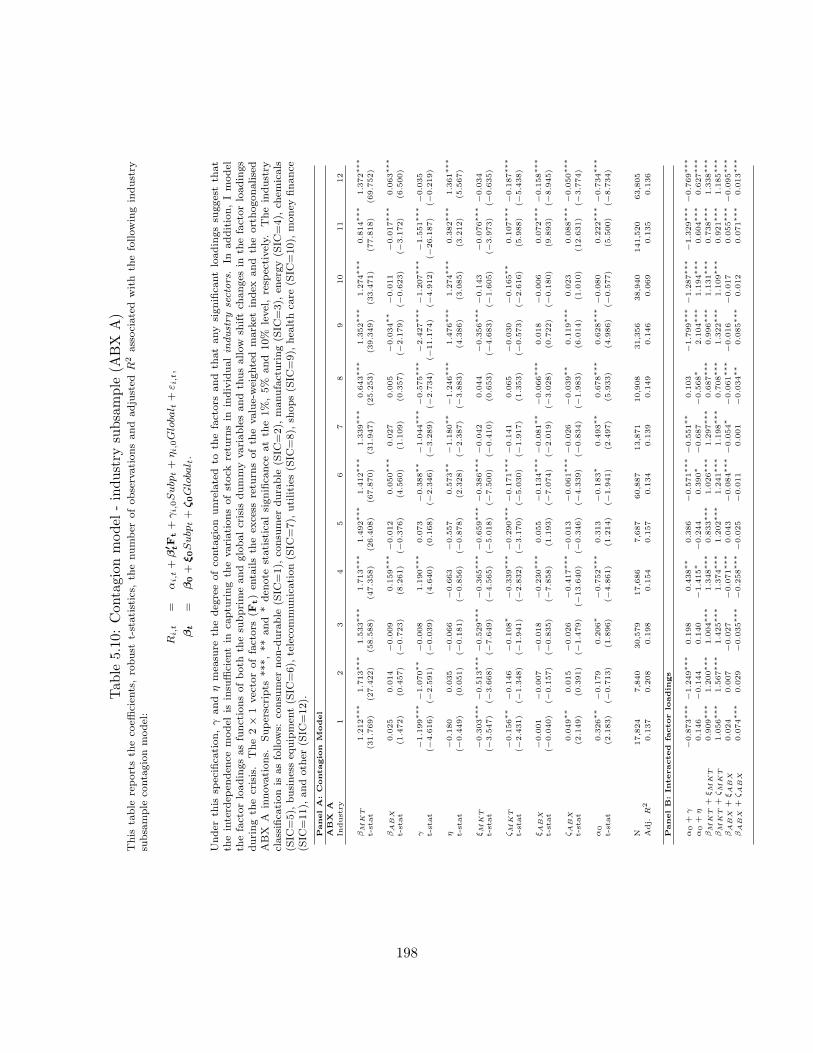
Tab
le5.10:Contagionmodel
-industry
subsample
(ABX
A)
This
table
reportsth
eco
efficien
ts,robust
t-statistics,
thenumber
ofobservationsand
adjusted
R2associated
with
thefollowingindustry
subsample
contagionmodel:
Ri,t
=αi,t+
β′ tF
t+
γi,0Subp
t+
ηi,0Globa
l t+
ε i,t,
βt
=β0+
ξ0Subp
t+
ζ0Globa
l t.
Under
this
specifica
tion,γ
and
ηmea
sure
thedeg
reeofco
ntagion
unrelated
toth
efactors
and
thatanysignifica
ntloadingssu
ggestth
at
theinterd
epen
den
cemodel
isinsu
fficien
tin
captu
ringth
evariationsofstock
retu
rnsin
individualindustry
sectors.
Inaddition,Imodel
thefactorloadingsasfunctionsofboth
thesu
bprimeandglobalcrisis
dummyvariablesandthusallow
shiftch
anges
inth
efactorloadings
duringth
ecrisis.
The2×
1vectoroffactors
(Ft)en
tailsth
eex
cess
retu
rnsofth
evalue-weighted
market
index
and
theorthogonalised
ABX
Ainnovations.
Superscripts
***,**and
*den
ote
statisticalsignifica
nce
atth
e1%,5%
and
10%
level,resp
ectively.
Theindustry
classifica
tionis
asfollows:
consu
mer
non-durable
(SIC
=1),
consu
mer
durable
(SIC
=2),
manufacturing(S
IC=3),
energy(S
IC=4),
chem
icals
(SIC
=5),
businesseq
uipmen
t(S
IC=6),
teleco
mmunication(S
IC=7),
utilities
(SIC
=8),
shops(S
IC=9),
hea
lthca
re(S
IC=10),
money
finance
(SIC
=11),
andoth
er(S
IC=12).
PanelA
:Contagio
nM
odel
ABX
A
Industry
12
34
56
78
910
11
12
βM
KT
1.212∗∗∗
1.713∗∗∗
1.533∗∗∗
1.713∗∗∗
1.492∗∗∗
1.412∗∗∗
1.339∗∗∗
0.643∗∗∗
1.352∗∗∗
1.274∗∗∗
0.814∗∗∗
1.372∗∗∗
t-stat
(31.769)
(27.422)
(58.588)
(47.358)
(26.408)
(67.870)
(31.947)
(25.253)
(39.349)
(33.471)
(77.818)
(69.752)
βA
BX
0.025
0.014
−0.009
0.159∗∗∗
−0.012
0.050∗∗∗
0.027
0.005
−0.034∗∗
−0.011
−0.017∗∗∗
0.063∗∗∗
t-stat
(1.472)
(0.457)
(−0.723)
(8.261)
(−0.376)
(4.560)
(1.109)
(0.357)
(−2.179)
(−0.623)
(−3.172)
(6.500)
γ−1.199∗∗∗
−1.070∗∗
−0.008
1.190∗∗∗
0.073
−0.388∗∗
−1.044∗∗∗
−0.575∗∗∗
−2.427∗∗∗
−1.207∗∗∗
−1.551∗∗∗
−0.035
t-stat
(−4.616)
(−2.591)
(−0.039)
(4.640)
(0.168)
(−2.346)
(−3.289)
(−2.734)
(−11.174)
(−4.912)
(−26.187)
(−0.219)
η−0.180
0.035
−0.066
−0.663
−0.557
0.573∗∗
−1.180∗∗
−1.246∗∗∗
1.476∗∗∗
1.274∗∗∗
0.382∗∗∗
1.361∗∗∗
t-stat
(−0.449)
(0.051)
(−0.181)
(−0.856)
(−0.878)
(2.328)
(−2.387)
(−3.883)
(4.386)
(3.085)
(3.212)
(5.567)
ξM
KT
−0.303∗∗∗
−0.513∗∗∗
−0.529∗∗∗
−0.365∗∗∗
−0.659∗∗∗
−0.386∗∗∗
−0.042
0.044
−0.356∗∗∗
−0.143
−0.076∗∗∗
−0.034
t-stat
(−3.547)
(−3.668)
(−7.649)
(−4.565)
(−5.018)
(−7.500)
(−0.410)
(0.653)
(−4.683)
(−1.605)
(−3.973)
(−0.635)
ζM
KT
−0.156∗∗
−0.146
−0.108∗
−0.339∗∗∗
−0.290∗∗∗
−0.171∗∗∗
−0.141
0.065
−0.030
−0.165∗∗
0.107∗∗∗
−0.187∗∗∗
t-stat
(−2.431)
(−1.348)
(−1.941)
(−2.832)
(−3.170)
(−5.030)
(−1.917)
(1.353)
(−0.573)
(−2.616)
(5.988)
(−5.438)
ξA
BX
−0.001
−0.007
−0.018
−0.230∗∗∗
0.055
−0.134∗∗∗
−0.081∗∗
−0.066∗∗∗
0.018
−0.006
0.072∗∗∗
−0.158∗∗∗
t-stat
(−0.040)
(−0.157)
(−0.835)
(−7.858)
(1.193)
(−7.074)
(−2.019)
(−3.028)
(0.722)
(−0.180)
(9.893)
(−8.945)
ζA
BX
0.049∗∗
0.015
−0.026
−0.417∗∗∗
−0.013
−0.061∗∗∗
−0.026
−0.039∗∗
0.119∗∗∗
0.023
0.088∗∗∗
−0.050∗∗∗
t-stat
(2.149)
(0.391)
(−1.479)
(−13.640)
(−0.346)
(−4.339)
(−0.834)
(−1.983)
(6.014)
(1.010)
(12.631)
(−3.774)
α0
0.326∗∗
−0.179
0.206∗
−0.752∗∗∗
0.313
−0.183∗
0.493∗∗
0.678∗∗∗
0.628∗∗∗
−0.080
0.222∗∗∗
−0.734∗∗∗
t-stat
(2.183)
(−0.713)
(1.896)
(−4.861)
(1.214)
(−1.941)
(2.497)
(5.933)
(4.986)
(−0.577)
(5.500)
(−8.734)
N17,824
7,840
30,579
17,686
7,687
60,887
13,871
10,908
31,356
38,940
141,520
63,805
Adj.
R2
0.137
0.208
0.198
0.154
0.157
0.134
0.139
0.149
0.146
0.069
0.135
0.136
PanelB:Interacted
factor
loadin
gs
α0+
γ−0.873∗∗∗
−1.249∗∗∗
0.198
0.438∗∗
0.386
−0.571∗∗∗
−0.551∗∗
0.103
−1.799∗∗∗
−1.287∗∗∗
−1.329∗∗∗
−0.769∗∗∗
α0+
η0.146
−0.144
0.140
−1.415∗
−0.244
0.390∗
−0.687
−0.568∗
2.104∗∗∗
1.194∗∗∗
0.604∗∗∗
0.627∗∗∗
βM
KT
+ξM
KT
0.909∗∗∗
1.200∗∗∗
1.004∗∗∗
1.348∗∗∗
0.833∗∗∗
1.026∗∗∗
1.297∗∗∗
0.687∗∗∗
0.996∗∗∗
1.131∗∗∗
0.738∗∗∗
1.338∗∗∗
βM
KT
+ζM
KT
1.056∗∗∗
1.567∗∗∗
1.425∗∗∗
1.374∗∗∗
1.202∗∗∗
1.241∗∗∗
1.198∗∗∗
0.708∗∗∗
1.322∗∗∗
1.109∗∗∗
0.921∗∗∗
1.185∗∗∗
βA
BX
+ξA
BX
0.024
0.007
−0.027
−0.071∗∗∗
0.043
−0.084∗∗∗
−0.054∗
−0.061∗∗∗
−0.016
−0.017
0.055∗∗∗
−0.095∗∗∗
βA
BX
+ζA
BX
0.074∗∗∗
0.029
−0.035∗∗∗
−0.258∗∗∗
−0.025
−0.011
0.001
−0.034∗∗
0.085∗∗∗
0.012
0.071∗∗∗
0.013∗∗∗
198

Tab
le5.11:Contagionmodel
-industry
subsample
(ABX
BBB)
This
table
reportsth
eco
efficien
ts,robust
t-statistics,
thenumber
ofobservationsand
adjusted
R2associated
with
thefollowingindustry
subsample
contagionmodel:
Ri,t
=αi,t+
β′ tF
t+
γi,0Subp
t+
ηi,0Globa
l t+
ε i,t,
βt
=β0+
ξ0Subp
t+
ζ0Globa
l t.
Under
this
specifica
tion,γ
and
ηmea
sure
thedeg
reeofco
ntagion
unrelated
toth
efactors
and
thatany
significa
ntloadingssu
ggestth
at
theinterd
epen
den
cemodel
isinsu
fficien
tin
captu
ringth
evariationsofstock
retu
rnsin
individualindustry
sectors.In
addition,Imodel
the
factorloadingsasfunctionsofboth
thesu
bprimeandglobalcrisis
dummyvariablesandthusallow
shiftch
anges
inth
efactorloadingsduring
thecrisis.The2×
1vectoroffactors
(Ft)en
tailsth
eex
cess
retu
rnsofth
evalue-weightedmarket
index
andth
eorthogonalisedABX
BBB
innovations.
Superscripts
***,**and*den
ote
statisticalsignifica
nce
at1%,5%
and10%
level
resp
ectively.
Theindustry
classifica
tionis
as
follows:
consu
mer
non-durable
(SIC
=1),
consu
mer
durable
(SIC
=2),
manufacturing(S
IC=3),
energy(S
IC=4),
chem
icals
(SIC
=5),
business
equipmen
t(S
IC=6),
teleco
mmunication
(SIC
=7),
utilities
(SIC
=8),
shops(S
IC=9),
hea
lth
care
(SIC
=10),
money
finance
(SIC
=11),
and
oth
er(S
IC=12).
PanelA
:Contagio
nm
odel
ABX
BBB
Industry
12
34
56
78
910
11
12
βM
KT
1.289∗∗∗
1.766∗∗∗
1.591∗∗∗
1.796∗∗∗
1.500∗∗∗
1.534∗∗∗
1.438∗∗∗
0.652∗∗∗
1.375∗∗∗
1.393∗∗∗
0.830∗∗∗
1.446∗∗∗
t-stat
(28.601)
(22.917)
(50.698)
(40.949)
(22.104)
(60.124)
(26.800)
(21.056)
(36.264)
(30.786)
(62.911)
(58.779)
βA
BX
0.134∗∗∗
0.089
0.080∗∗∗
0.245∗∗∗
0.004
0.222∗∗∗
0.168∗∗∗
0.016
0.010
0.168∗∗∗
0.012
0.158∗∗∗
t-stat
(3.447)
(1.264)
(2.827)
(6.205)
(0.070)
(9.411)
(3.225)
(0.577)
(0.283)
(4.607)
(0.881)
(6.946)
γ−0.140
−0.358
0.733∗∗∗
2.088∗∗∗
0.628
0.648∗∗∗
−0.158
−0.597∗∗
−2.004∗∗∗
−0.207
−1.239∗∗∗
0.478∗∗
t-stat
(−0.410)
(−0.647)
(2.868)
(6.032)
(1.093)
(2.979)
(−0.379)
(−2.172)
(−6.967)
(−0.655)
(−14.011)
(2.305)
η0.567
0.304
0.433
0.123
−0.269
1.892∗∗∗
−0.340
−1.257∗∗∗
2.094∗∗∗
2.666∗∗∗
0.617∗∗∗
1.966∗∗∗
t-stat
(1.208)
(0.375)
(1.013)
(0.136)
(−0.360)
(6.540)
(−0.578)
(−3.446)
(5.241)
(5.504)
(4.351)
(6.955)
ξM
KT
−0.532∗∗∗
−0.665∗∗∗
−0.679∗∗∗
−0.510∗∗∗
−0.842∗∗∗
−0.514∗∗∗
−0.165
0.075
−0.458∗∗∗
−0.274∗∗
−0.161∗∗∗
−0.061
t-stat
(−5.293)
(−4.085)
(−8.842)
(−5.294)
(−5.401)
(−8.263)
(−1.299)
(0.975)
(−5.368)
(−2.467)
(−7.028)
(−0.958)
ζM
KT
−0.221∗∗
−0.203∗
−0.167∗∗∗
−0.440∗∗∗
−0.291∗∗∗
−0.279∗∗∗
−0.238∗∗∗
0.049
−0.026
−0.263∗∗∗
0.104∗∗∗
−0.260∗∗∗
t-stat
(−3.204)
(−1.717)
(−2.826)
(−3.509)
(−2.920)
(−7.447)
(−2.901)
(0.960)
(−0.483)
(−3.818)
(5.256)
(−6.897)
ξA
BX
−0.055
−0.040
−0.041
−0.228∗∗∗
0.088
−0.236∗∗∗
−0.167∗∗∗
−0.048
0.025
−0.165∗∗∗
0.033∗∗
−0.199∗∗∗
t-stat
(−1.238)
(−0.514)
(−1.270)
(−5.108)
(1.304)
(−8.628)
(−2.811)
(−1.466)
(0.659)
(−3.681)
(2.341)
(−7.553)
ζA
BX
−0.052
−0.077
−0.110∗∗∗
−0.480∗∗∗
−0.007
−0.201∗∗∗
−0.163∗∗∗
−0.056∗
0.110∗∗∗
−0.115∗∗∗
0.065∗∗∗
−0.146∗∗∗
t-stat
(−1.212)
(−1.017)
(−3.541)
(−10.609)
(−0.106)
(−7.836)
(−2.815)
(−1.698)
(3.034)
(−2.873)
(4.576)
(−5.825)
α0
−0.297
−0.605
−0.260
−1.437∗∗∗
0.243
−1.173∗∗∗
−0.307
0.607∗∗∗
0.436∗∗
−1.039∗∗∗
0.091
−1.347∗∗∗
t-stat
(−1.227)
(−1.434)
(−1.473)
(−5.708)
(0.585)
(−7.570)
(−0.979)
(3.241)
(2.033)
(−4.672)
(1.231)
(−9.520)
N17,824
7,840
30,579
17,686
7,687
60,887
13,871
10,908
31,356
38,940
141,520
63,805
Adj.
R2
0.138
0.208
0.198
0.149
0.158
0.134
0.139
0.148
0.147
0.069
0.135
0.136
PanelB:Interacted
factor
loadin
gs
α0+
γ−0.437∗
−0.963∗∗∗
0.473∗∗
0.651∗∗∗
0.871∗∗
−0.525∗∗∗
−0.465∗
0.010
−1.568∗∗∗
−1.246∗∗∗
−1.148∗∗∗
−0.869∗∗∗
α0+
η0.270
−0.301
0.173
−1.314
−0.026
0.719∗∗∗
−0.647
−0.650∗∗
2.530∗∗∗
1.627∗∗∗
0.708∗∗∗
0.619∗∗
βM
KT
+ξM
KT
0.757∗∗∗
1.101∗∗∗
0.912∗∗∗
1.286∗∗∗
0.658∗∗∗
1.020∗∗∗
1.273∗∗∗
0.727∗∗∗
0.917∗∗∗
1.119∗∗∗
0.669∗∗∗
1.385∗∗∗
βM
KT
+ζM
KT
1.068∗∗∗
1.563∗∗∗
1.424∗∗∗
1.356∗∗∗
1.209∗∗∗
1.255∗∗∗
1.200∗∗∗
0.701∗∗∗
1.349∗∗∗
1.130∗∗∗
0.934∗∗∗
1.186∗∗∗
βA
BX
+ξA
BX
0.079∗∗∗
0.049
0.039
0.017
0.092∗∗∗
−0.014
0.001
−0.032∗
0.035∗∗
0.003
0.045∗∗∗
−0.041∗∗∗
βA
BX
+ζA
BX
0.082∗∗∗
0.012
−0.030∗∗
−0.235∗∗∗
−0.003
0.021∗∗
0.005
−0.040∗∗
0.120∗∗∗
0.053∗∗∗
0.077∗∗∗
0.012
199
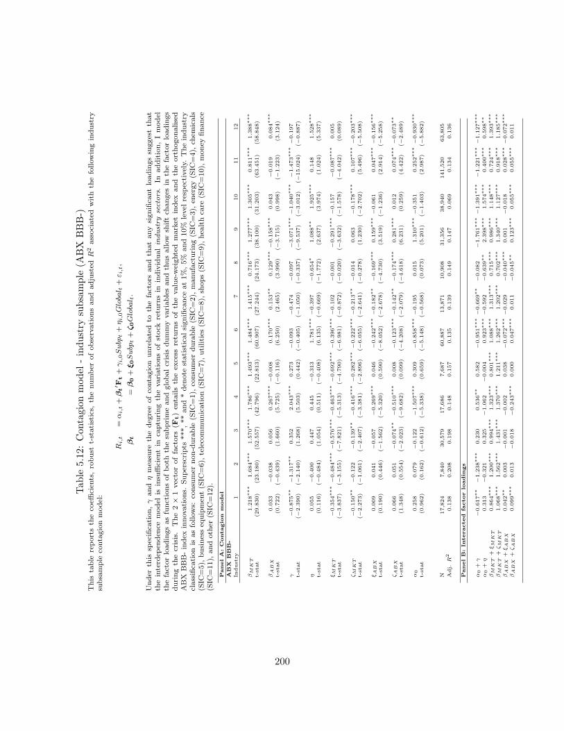
Tab
le5.12:Contagionmodel
-industry
subsample
(ABX
BBB-)
This
table
reportsth
eco
efficien
ts,robust
t-statistics,
thenumber
ofobservationsand
adjusted
R2associated
with
thefollowingindustry
subsample
contagionmodel:
Ri,t
=αi,t+
βt′ F
t+
γi,0Subp
t+
ηi,0Globa
l t+
ε i,t,
βt
=β0+
ξ0Subp
t+
ζ0Globa
l t.
Under
this
specifica
tion,γ
and
ηmea
sure
thedeg
reeofco
ntagion
unrelated
toth
efactors
and
thatanysignifica
ntloadingssu
ggestth
at
theinterd
epen
den
cemodel
isinsu
fficien
tin
captu
ringth
evariationsofstock
retu
rnsin
individualindustry
sectors.
Inaddition,Imodel
thefactorloadingsasfunctionsofboth
thesu
bprimeandglobalcrisis
dummyvariablesandthusallow
shiftch
anges
inth
efactorloadings
duringth
ecrisis.
The2×
1vectoroffactors
(Ft)en
tailsth
eex
cess
retu
rnsofth
evalue-weighted
market
index
and
theorthogonalised
ABX
BBB-index
innovations.
Superscripts
***,**and*den
ote
statisticalsignifica
nce
at1%,5%
and10%
level
resp
ectively.
Theindustry
classifica
tionis
asfollows:
consu
mer
non-durable
(SIC
=1),
consu
mer
durable
(SIC
=2),
manufacturing(S
IC=3),
energy(S
IC=4),
chem
icals
(SIC
=5),
businesseq
uipmen
t(S
IC=6),
teleco
mmunication(S
IC=7),
utilities
(SIC
=8),
shops(S
IC=9),
hea
lthca
re(S
IC=10),
money
finance
(SIC
=11),
andoth
er(S
IC=12).
PanelA
:Contagio
nm
odel
ABX
BBB-
Industry
12
34
56
78
910
11
12
βM
KT
1.218∗∗∗
1.684∗∗∗
1.570∗∗∗
1.786∗∗∗
1.493∗∗∗
1.484∗∗∗
1.415∗∗∗
0.716∗∗∗
1.277∗∗∗
1.305∗∗∗
0.811∗∗∗
1.388∗∗∗
t-stat
(29.830)
(23.180)
(52.557)
(42.796)
(22.813)
(60.907)
(27.244)
(24.173)
(38.100)
(31.203)
(63.451)
(58.848)
βA
BX
0.033
−0.038
0.056
0.267∗∗∗
−0.008
0.170∗∗∗
0.153∗∗
0.129∗∗∗
−0.158∗∗∗
0.043
−0.019
0.084∗∗∗
t-stat
(0.722)
(−0.439)
(1.660)
(5.725)
(−0.116)
(6.250)
(2.465)
(3.990)
(−3.715)
(0.998)
(−1.223)
(3.124)
γ−0.875∗∗
−1.317∗∗
0.352
2.043∗∗∗
0.273
−0.093
−0.474
−0.097
−3.071∗∗∗
−1.040∗∗∗
−1.473∗∗∗
−0.197
t-stat
(−2.390)
(−2.140)
(1.268)
(5.503)
(0.442)
(−0.405)
(−1.050)
(−0.337)
(−9.537)
(−3.012)
(−15.024)
(−0.887)
η0.055
−0.400
0.447
0.445
−0.313
1.781∗∗∗
−0.397
−0.654∗
1.088∗∗
1.925∗∗∗
0.148
1.528∗∗∗
t-stat
(0.116)
(−0.484)
(1.054)
(0.511)
(−0.408)
(6.135)
(−0.669)
(−1.772)
(2.637)
(3.974)
(1.024)
(5.337)
ξM
KT
−0.354∗∗∗
−0.484∗∗∗
−0.576∗∗∗
−0.463∗∗∗
−0.692∗∗∗
−0.396∗∗∗
−0.102
−0.001
−0.291∗∗∗
−0.157
−0.087∗∗∗
0.005
t-stat
(−3.837)
(−3.155)
(−7.821)
(−5.313)
(−4.790)
(−6.981)
(−0.872)
(−0.020)
(−3.632)
(−1.578)
(−4.042)
(0.089)
ζM
KT
−0.150∗∗
−0.122
−0.139∗∗
−0.416∗∗∗
−0.282∗∗∗
−0.222∗∗∗
−0.213∗∗
−0.014
0.063
−0.178∗∗∗
0.107∗∗∗
−0.203∗∗∗
t-stat
(−2.273)
(−1.061)
(−2.407)
(−3.381)
(−2.896)
(−6.055)
(−2.641)
(−0.278)
(1.230)
(−2.702)
(5.496)
(−5.508)
ξA
BX
0.009
0.041
−0.057
−0.269∗∗∗
0.046
−0.242∗∗∗
−0.182∗∗
−0.169∗∗∗
0.159∗∗∗
−0.061
0.047∗∗∗
−0.156∗∗∗
t-stat
(0.190)
(0.446)
(−1.562)
(−5.320)
(0.590)
(−8.052)
(−2.678)
(−4.730)
(3.519)
(−1.236)
(2.914)
(−5.258)
ζA
BX
0.066
0.051
−0.074∗∗
−0.510∗∗∗
0.008
−0.123∗∗∗
−0.142∗∗
−0.174∗∗∗
0.281∗∗∗
0.012
0.074∗∗∗
−0.073∗∗
t-stat
(1.348)
(0.554)
(−2.023)
(−9.682)
(0.099)
(−4.208)
(−2.079)
(−4.618)
(6.231)
(0.259)
(4.422)
(−2.489)
α0
0.258
0.079
−0.122
−1.507∗∗∗
0.309
−0.858∗∗∗
−0.195
0.015
1.310∗∗∗
−0.351
0.252∗∗∗
−0.930∗∗∗
t-stat
(0.962)
(0.162)
(−0.612)
(−5.338)
(0.659)
(−5.148)
(−0.568)
(0.073)
(5.201)
(−1.403)
(2.987)
(−5.882)
N17,824
7,840
30,579
17,686
7,687
60,887
13,871
10,908
31,356
38,940
141,520
63,805
Adj.
R2
0.138
0.208
0.198
0.148
0.157
0.135
0.139
0.149
0.147
0.069
0.134
0.136
PanelB:Interacted
factor
loadin
gs
α0+
γ−0.617∗∗
−1.238∗∗∗
0.230
0.536∗∗
0.582
−0.951∗∗∗
−0.669∗∗
−0.082
−1.761∗∗∗
−1.391∗∗∗
−1.221∗∗∗
−1.127∗∗∗
α0+
η0.313
−0.321
0.325
−1.062
−0.004
0.923∗∗∗
−0.592
−0.639∗∗
2.398∗∗∗
1.574∗∗∗
0.400∗∗∗
0.598∗∗
βM
KT
+ξM
KT
0.864∗∗∗
1.200∗∗∗
0.994∗∗∗
1.323∗∗∗
0.801∗∗∗
1.088∗∗∗
1.313∗∗∗
0.715∗∗∗
0.986∗∗∗
1.148∗∗∗
0.724∗∗∗
1.393∗∗∗
βM
KT
+ζM
KT
1.068∗∗∗
1.562∗∗∗
1.431∗∗∗
1.370∗∗∗
1.211∗∗∗
1.262∗∗∗
1.202∗∗∗
0.702∗∗∗
1.340∗∗∗
1.127∗∗∗
0.918∗∗∗
1.185∗∗∗
βA
BX
+ξA
BX
0.042∗∗
0.003
−0.001
−0.002
0.038
−0.072∗∗∗
−0.029
−0.040∗∗∗
0.001
−0.018
0.028∗∗∗
−0.072∗∗∗
βA
BX
+ζA
BX
0.099∗∗∗
0.013
−0.018
−0.243∗∗∗
0.000
0.047∗∗∗
0.011
−0.045∗∗
0.123∗∗∗
0.055∗∗∗
0.055∗∗∗
0.011
200
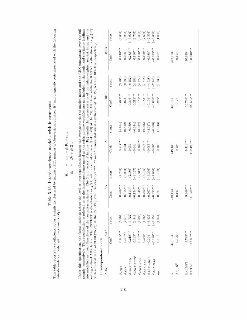
Table
5.13:Interdep
endence
model
-withinstruments
This
table
reportsth
eco
efficien
ts,robust
t-statisticsclustered
byindustry
SIC
,number
ofobservations,
adjusted
R2anddiagnostic
testsassociatedwithth
efollowing
interd
epen
den
cemodel
withinstru
men
ts(Z
t):
Ri,t
=αi,t+
β′ tF
t+
ε i,t,
βt
=β0+
ϕ1Zt.
Under
this
specifica
tion,th
efactorloadingsreflectth
elevel
ofinterd
epen
den
cebetween
theaveragestock
,th
emarket
index
and
theABX
innovationsover
thefull
sample,resp
ectively.
This
specifica
tionis
referred
toasth
einterd
epen
den
cemodel
asth
ecrisis
dummyvariablesare
notincluded
inth
emodel
andth
efactorloadings
are
modelled
aslinea
rfunctionsofth
eco
ntagion
variables.
The2×
1vectoroffactors
(Ft)en
tailsth
eex
cess
retu
rnsofth
evalue-weighted
market
index
and
the
orthogonalisedABX
factor.
TheEXTEST
isdistributedasχ2(1)withacriticalvalueof3.84(6.63)atth
e5%
(1%)level
whileth
eIC
STAT
isdistributedasχ2(12)
withacriticalvalueof21.03(26.22)atth
e5%
(1%)level.Superscripts
***,**and*den
ote
statisticalsignifica
nce
atth
e1%,5%
and10%
level
resp
ectively.
Inte
rdependencem
odel
ABX
AAA
AA
ABBB
BBB-
Coef.
t-stat
Coef.
t-stat
Coef.
t-stat
Coef.
t-stat
Coef.
t-stat
βM
KT
0.805∗∗
∗(5.564)
0.966∗∗
∗(7.238)
0.817∗∗
∗(5.164)
0.672∗∗
∗(3.905)
0.746∗∗
∗(4.601)
βABX
0.467∗∗
(2.616)
0.318∗∗
∗(6.063)
0.031
(0.812)
0.023
(0.686)
0.008
(0.233)
ϕM
KT,T
ED
−0.219∗∗
∗(−
3.722)
0.114∗∗
(2.386)
−0.054
(−0.980)
−0.346∗∗
∗(−
6.482)
−0.282∗∗
∗(−
5.002)
ϕM
KT,A
BCP
0.143∗∗
(2.342)
−0.154∗∗
∗(−
3.127)
−0.043
(−0.944)
0.211∗∗
∗(4.483)
0.196∗∗
(2.705)
ϕM
KT,B
AA
0.107∗∗
∗(4.096)
0.049∗∗
(2.317)
0.104∗∗
∗(3.937)
0.151∗∗
∗(4.372)
0.120∗∗
∗(3.832)
ϕABX
,TED
0.368∗
(1.868)
0.262∗∗
∗(3.795)
0.078∗∗
(2.096)
0.183∗∗
∗(7.848)
0.190∗∗
∗(7.601)
ϕABX
,ABCP
−0.204
(−1.427)
−0.207∗∗
∗(−
5.296)
−0.083∗∗
∗(−
4.047)
−0.104∗∗
∗(−
4.038)
−0.088∗∗
(−2.593)
ϕABX
,BAA
−0.126∗∗
(−2.159)
−0.093∗∗
∗(−
4.696)
−0.005
(−0.366)
−0.030∗∗
∗(−
7.446)
−0.033∗∗
∗(−
6.609)
α0
0.101
(1.041)
−0.021
(−0.199)
0.109
(1.043)
0.269∗
(1.930)
0.297
(1.808)
N443,188
443,188
443,188
443,188
443,188
Adj.
R2
0.126
0.127
0.126
0.127
0.127
EXTEST
9.785∗∗
∗9.266∗∗
∗9.414∗∗
∗10.730∗∗
∗10.829
ICSTAT
117.897∗∗
∗111.989∗∗
∗112.490∗∗
∗129.506∗∗
∗130.040∗∗
∗
201
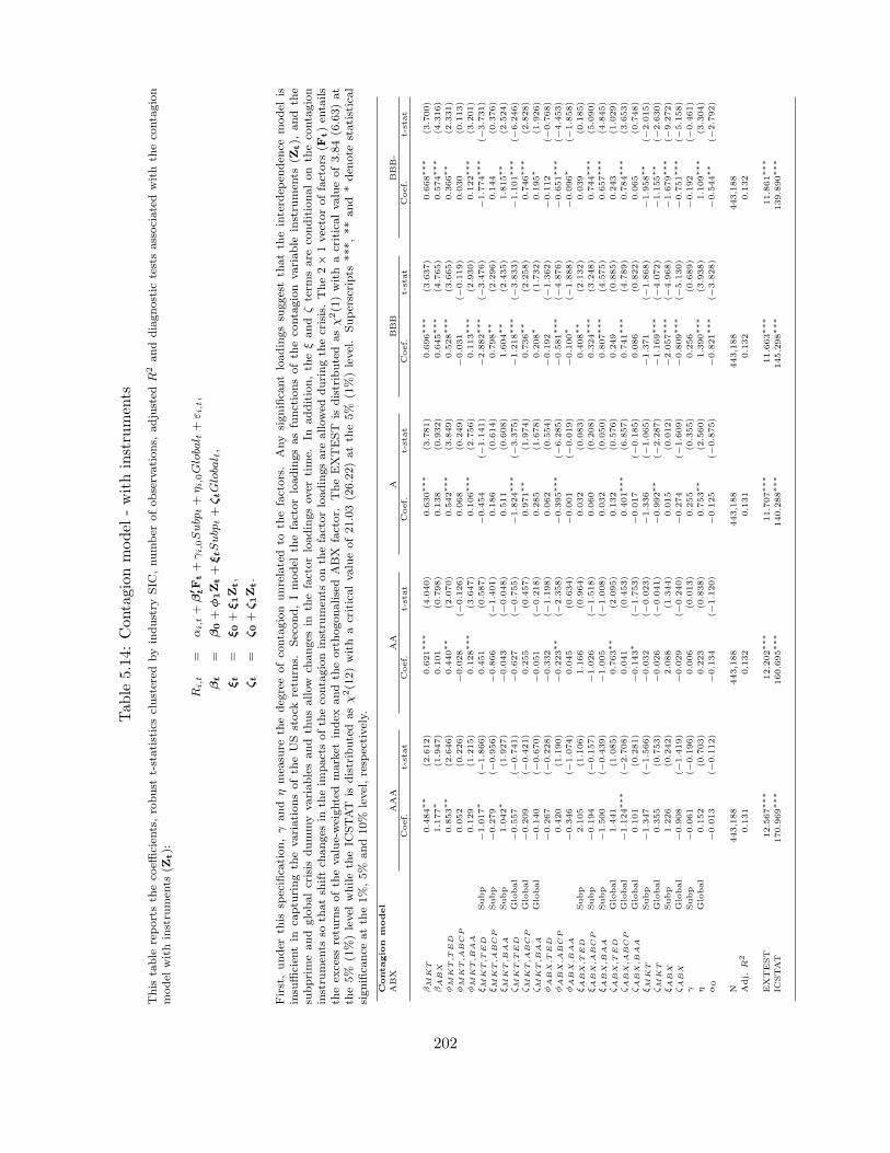
Table
5.14:Contagionmodel
-withinstruments
This
table
reportsth
eco
efficien
ts,robust
t-statisticsclustered
byindustry
SIC
,number
ofobservations,
adjusted
R2anddiagnostic
testsassociatedwithth
eco
ntagion
model
withinstru
men
ts(Z
t):
Ri,t
=αi,t+
β′ tF
t+
γi,0Subp
t+
ηi,0Globa
l t+
ε i,t,
βt
=β0+
ϕ1Zt+
ξtSubp
t+
ζtGloba
l t,
ξt
=ξ0+
ξ1Zt,
ζt
=ζ0+
ζ1Zt.
First,under
this
specifica
tion,γ
and
ηmea
sure
thedeg
reeofco
ntagion
unrelated
toth
efactors.
Any
significa
ntloadingssu
ggestth
atth
einterd
epen
den
cemodel
isinsu
fficien
tin
captu
ringth
evariationsofth
eUS
stock
retu
rns.
Second,Imodel
thefactorloadingsasfunctionsofth
eco
ntagion
variable
instru
men
ts(Z
t),
and
the
subprimeand
globalcrisis
dummyvariablesand
thusallow
changes
inth
efactorloadingsover
time.
Inaddition,th
eξand
ζterm
sare
conditionalon
theco
ntagion
instru
men
tsso
thatsh
iftch
anges
inth
eim
pactsofth
eco
ntagioninstru
men
tsonth
efactorloadingsare
allowed
duringth
ecrisis.The2×
1vectoroffactors
(Ft)en
tails
theex
cess
retu
rnsofth
evalue-weighted
market
index
and
theorthogonalised
ABX
factor.
TheEXTEST
isdistributed
asχ2(1)with
acriticalvalueof3.84(6.63)at
the5%
(1%)level
whileth
eIC
STAT
isdistributed
asχ2(12)with
acriticalvalueof21.03(26.22)atth
e5%
(1%)level.Superscripts
***,**and
*den
ote
statistical
significa
nce
atth
e1%,5%
and10%
level,resp
ectively.
Contagio
nm
odel
ABX
AAA
AA
ABBB
BBB-
Coef.
t-stat
Coef.
t-stat
Coef.
t-stat
Coef.
t-stat
Coef.
t-stat
βM
KT
0.484∗∗
(2.612)
0.621∗∗∗
(4.040)
0.630∗∗∗
(3.781)
0.696∗∗∗
(3.637)
0.668∗∗∗
(3.700)
βA
BX
1.177∗
(1.947)
0.101
(0.798)
0.138
(0.932)
0.645∗∗∗
(4.765)
0.574∗∗∗
(4.316)
ϕM
KT,T
ED
0.853∗∗
(2.646)
0.440∗∗
(2.070)
0.542∗∗∗
(3.849)
0.528∗∗∗
(3.665)
0.366∗∗
(2.331)
ϕM
KT,A
BC
P0.052
(0.226)
−0.028
(−0.126)
0.068
(0.249)
−0.031
(−0.119)
0.030
(0.113)
ϕM
KT,B
AA
0.129
(1.215)
0.128∗∗∗
(3.647)
0.106∗∗∗
(2.756)
0.113∗∗∗
(2.930)
0.122∗∗∗
(3.201)
ξM
KT,T
ED
Subp
−1.017∗
(−1.866)
0.451
(0.587)
−0.454
(−1.141)
−2.882∗∗∗
(−3.476)
−1.774∗∗∗
(−3.731)
ξM
KT,A
BC
PSubp
−0.279
(−0.956)
−0.866
(−1.401)
0.186
(0.614)
0.798∗∗
(2.296)
0.144
(0.376)
ξM
KT,B
AA
Subp
1.042∗
(1.927)
−0.043
(−0.048)
0.511
(0.608)
1.604∗∗
(2.435)
1.815∗∗
(2.524)
ζM
KT,T
ED
Global
−0.557
(−0.741)
−0.627
(−0.755)
−1.824∗∗∗
(−3.375)
−1.218∗∗∗
(−3.833)
−1.101∗∗∗
(−6.246)
ζM
KT,A
BC
PGlobal
−0.209
(−0.421)
0.255
(0.457)
0.971∗∗
(1.974)
0.736∗∗
(2.258)
0.746∗∗∗
(2.828)
ζM
KT,B
AA
Global
−0.140
(−0.670)
−0.051
(−0.218)
0.285
(1.678)
0.208∗
(1.732)
0.195∗
(1.926)
ϕA
BX
,TE
D−0.267
(−0.228)
−0.332
(−1.198)
0.062
(0.554)
−0.192
(−1.362)
−0.112
(−0.768)
ϕA
BX
,AB
CP
0.420
(1.190)
−0.223∗∗
(−2.358)
−0.395∗∗∗
(−6.285)
−0.581∗∗∗
(−4.876)
−0.651∗∗∗
(−4.453)
ϕA
BX
,BA
A−0.346
(−1.074)
0.045
(0.634)
−0.001
(−0.019)
−0.100∗
(−1.888)
−0.096∗
(−1.858)
ξA
BX
,TE
DSubp
2.105
(1.106)
1.166
(0.964)
0.032
(0.083)
0.408∗∗
(2.132)
0.039
(0.185)
ξA
BX
,AB
CP
Subp
−0.194
(−0.157)
−1.026
(−1.518)
0.060
(0.208)
0.324∗∗∗
(3.248)
0.744∗∗∗
(5.090)
ξA
BX
,BA
ASubp
−1.500
(−0.439)
−1.005
(−1.008)
0.032
(0.050)
0.807∗∗∗
(4.575)
0.657∗∗∗
(4.845)
ζA
BX
,TE
DGlobal
1.441
(1.085)
0.763∗∗
(2.095)
0.132
(0.576)
0.249
(0.885)
0.243
(1.029)
ζA
BX
,AB
CP
Global
−1.124∗∗∗
(−2.708)
0.041
(0.453)
0.401∗∗∗
(6.857)
0.741∗∗∗
(4.789)
0.784∗∗∗
(3.653)
ζA
BX
,BA
AGlobal
0.101
(0.281)
−0.143∗
(−1.753)
−0.017
(−0.185)
0.086
(0.822)
0.065
(0.748)
ξM
KT
Subp
−1.347
(−1.566)
−0.032
(−0.023)
−1.336
(−1.065)
−1.371
(−1.868)
−1.958∗∗
(−2.015)
ζM
KT
Global
0.355
(0.753)
−0.026
(−0.041)
−0.992∗∗
(−2.287)
−1.169∗∗∗
(−4.072)
−1.155∗∗
(−2.630)
ξA
BX
Subp
1.226
(0.242)
2.088
(1.344)
0.015
(0.012)
−2.057∗∗∗
(−4.968)
−1.679∗∗∗
(−9.272)
ζA
BX
Global
−0.908
(−1.419)
−0.029
(−0.240)
−0.274
(−1.609)
−0.809∗∗∗
(−5.130)
−0.751∗∗∗
(−5.158)
γSubp
−0.061
(−0.196)
0.006
(0.013)
0.255
(0.355)
0.256
(0.689)
−0.192
(−0.461)
ηGlobal
0.152
(0.703)
0.223
(0.838)
0.753∗∗
(2.560)
1.390∗∗∗
(3.938)
1.109∗∗∗
(3.304)
α0
−0. 013
( −0.112)
−0.134
(−1. 120)
−0. 125
( −0.875)
−0.821∗∗∗
( −3.828)
−0.544∗∗
( −2.792)
N443,188
443,188
443,188
443,188
443,188
Adj.
R2
0.131
0.132
0.131
0.132
0.132
EXTEST
12.567∗∗∗
12.202∗∗∗
11.707∗∗∗
11.663∗∗∗
11.861∗∗∗
ICSTAT
170.969∗∗∗
160.695∗∗∗
140.288∗∗∗
145.298∗∗∗
139.890∗∗∗
202
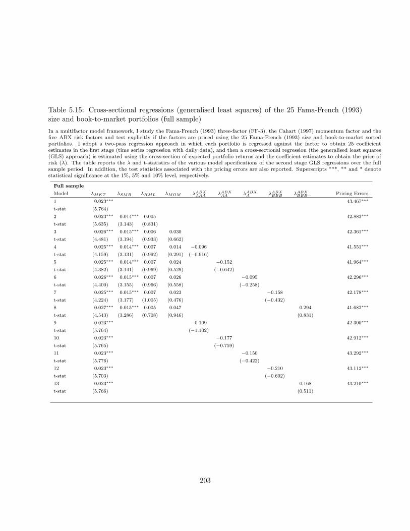
Table 5.15: Cross-sectional regressions (generalised least squares) of the 25 Fama-French (1993)size and book-to-market portfolios (full sample)
In a multifactor model framework, I study the Fama-French (1993) three-factor (FF-3), the Cahart (1997) momentum factor and thefive ABX risk factors and test explicitly if the factors are priced using the 25 Fama-French (1993) size and book-to-market sortedportfolios. I adopt a two-pass regression approach in which each portfolio is regressed against the factor to obtain 25 coefficientestimates in the first stage (time series regression with daily data), and then a cross-sectional regression (the generalised least squares(GLS) approach) is estimated using the cross-section of expected portfolio returns and the coefficient estimates to obtain the price ofrisk (λ). The table reports the λ and t-statistics of the various model specifications of the second stage GLS regressions over the fullsample period. In addition, the test statistics associated with the pricing errors are also reported. Superscripts ***, ** and * denotestatistical significance at the 1%, 5% and 10% level, respectively.
Full sample
Model λMKT λSMB λHML λMOM λABXAAA λABX
AA λABXA λABX
BBB λABXBBB− Pricing Errors
1 0.023∗∗∗ 43.467∗∗∗
t-stat (5.764)
2 0.023∗∗∗ 0.014∗∗∗ 0.005 42.883∗∗∗
t-stat (5.635) (3.143) (0.831)
3 0.026∗∗∗ 0.015∗∗∗ 0.006 0.030 42.361∗∗∗
t-stat (4.481) (3.194) (0.933) (0.662)
4 0.025∗∗∗ 0.014∗∗∗ 0.007 0.014 −0.096 41.551∗∗∗
t-stat (4.159) (3.131) (0.992) (0.291) (−0.916)
5 0.025∗∗∗ 0.014∗∗∗ 0.007 0.024 −0.152 41.964∗∗∗
t-stat (4.382) (3.141) (0.969) (0.529) (−0.642)
6 0.026∗∗∗ 0.015∗∗∗ 0.007 0.026 −0.095 42.296∗∗∗
t-stat (4.400) (3.155) (0.966) (0.558) (−0.258)
7 0.025∗∗∗ 0.015∗∗∗ 0.007 0.023 −0.158 42.178∗∗∗
t-stat (4.224) (3.177) (1.005) (0.476) (−0.432)
8 0.027∗∗∗ 0.015∗∗∗ 0.005 0.047 0.294 41.682∗∗∗
t-stat (4.543) (3.286) (0.708) (0.946) (0.831)
9 0.023∗∗∗ −0.109 42.300∗∗∗
t-stat (5.764) (−1.102)
10 0.023∗∗∗ −0.177 42.912∗∗∗
t-stat (5.765) (−0.759)
11 0.023∗∗∗ −0.150 43.292∗∗∗
t-stat (5.776) (−0.422)
12 0.023∗∗∗ −0.210 43.112∗∗∗
t-stat (5.703) (−0.602)
13 0.023∗∗∗ 0.168 43.210∗∗∗
t-stat (5.766) (0.511)
203
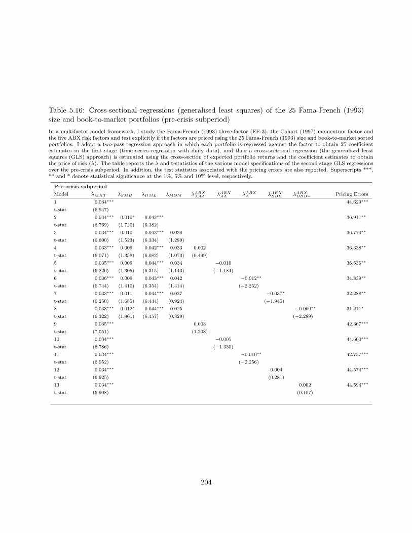
Table 5.16: Cross-sectional regressions (generalised least squares) of the 25 Fama-French (1993)size and book-to-market portfolios (pre-crisis subperiod)
In a multifactor model framework, I study the Fama-French (1993) three-factor (FF-3), the Cahart (1997) momentum factor andthe five ABX risk factors and test explicitly if the factors are priced using the 25 Fama-French (1993) size and book-to-market sortedportfolios. I adopt a two-pass regression approach in which each portfolio is regressed against the factor to obtain 25 coefficientestimates in the first stage (time series regression with daily data), and then a cross-sectional regression (the generalised leastsquares (GLS) approach) is estimated using the cross-section of expected portfolio returns and the coefficient estimates to obtainthe price of risk (λ). The table reports the λ and t-statistics of the various model specifications of the second stage GLS regressionsover the pre-crisis subperiod. In addition, the test statistics associated with the pricing errors are also reported. Superscripts ***,** and * denote statistical significance at the 1%, 5% and 10% level, respectively.
Pre-crisis subperiod
Model λMKT λSMB λHML λMOM λABXAAA λABX
AA λABXA λABX
BBB λABXBBB− Pricing Errors
1 0.034∗∗∗ 44.629∗∗∗
t-stat (6.947)
2 0.034∗∗∗ 0.010∗ 0.043∗∗∗ 36.911∗∗
t-stat (6.769) (1.720) (6.382)
3 0.034∗∗∗ 0.010 0.043∗∗∗ 0.038 36.770∗∗
t-stat (6.600) (1.523) (6.334) (1.289)
4 0.033∗∗∗ 0.009 0.042∗∗∗ 0.033 0.002 36.338∗∗
t-stat (6.071) (1.358) (6.082) (1.073) (0.499)
5 0.035∗∗∗ 0.009 0.044∗∗∗ 0.034 −0.010 36.535∗∗
t-stat (6.226) (1.305) (6.315) (1.143) (−1.184)
6 0.036∗∗∗ 0.009 0.043∗∗∗ 0.042 −0.012∗∗ 34.839∗∗
t-stat (6.744) (1.410) (6.354) (1.414) (−2.252)
7 0.033∗∗∗ 0.011 0.044∗∗∗ 0.027 −0.037∗ 32.288∗∗
t-stat (6.250) (1.685) (6.444) (0.924) (−1.945)
8 0.033∗∗∗ 0.012∗ 0.044∗∗∗ 0.025 −0.060∗∗ 31.211∗
t-stat (6.322) (1.861) (6.457) (0.829) (−2.289)
9 0.035∗∗∗ 0.003 42.367∗∗∗
t-stat (7.051) (1.208)
10 0.034∗∗∗ −0.005 44.600∗∗∗
t-stat (6.786) (−1.330)
11 0.034∗∗∗ −0.010∗∗ 42.757∗∗∗
t-stat (6.952) (−2.256)
12 0.034∗∗∗ 0.004 44.574∗∗∗
t-stat (6.925) (0.281)
13 0.034∗∗∗ 0.002 44.594∗∗∗
t-stat (6.908) (0.107)
204
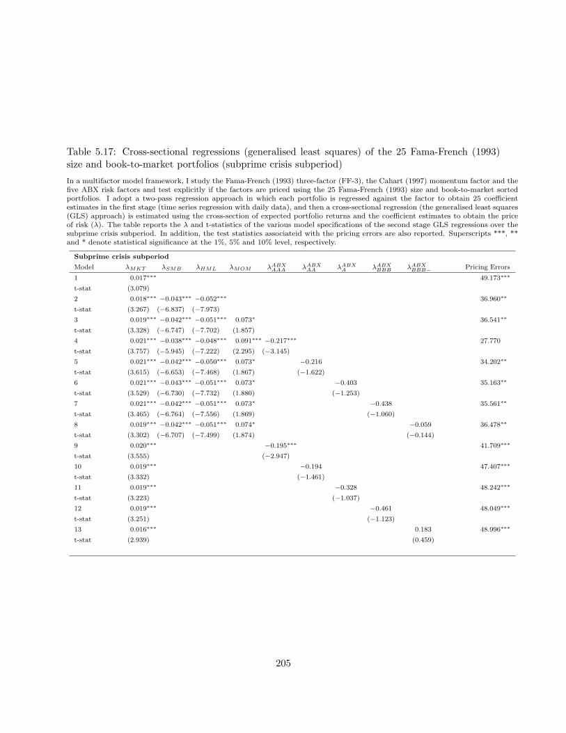
Table 5.17: Cross-sectional regressions (generalised least squares) of the 25 Fama-French (1993)size and book-to-market portfolios (subprime crisis subperiod)
In a multifactor model framework, I study the Fama-French (1993) three-factor (FF-3), the Cahart (1997) momentum factor and thefive ABX risk factors and test explicitly if the factors are priced using the 25 Fama-French (1993) size and book-to-market sortedportfolios. I adopt a two-pass regression approach in which each portfolio is regressed against the factor to obtain 25 coefficientestimates in the first stage (time series regression with daily data), and then a cross-sectional regression (the generalised least squares(GLS) approach) is estimated using the cross-section of expected portfolio returns and the coefficient estimates to obtain the priceof risk (λ). The table reports the λ and t-statistics of the various model specifications of the second stage GLS regressions over thesubprime crisis subperiod. In addition, the test statistics associateid with the pricing errors are also reported. Superscripts ***, **and * denote statistical significance at the 1%, 5% and 10% level, respectively.
Subprime crisis subperiod
Model λMKT λSMB λHML λMOM λABXAAA λABX
AA λABXA λABX
BBB λABXBBB− Pricing Errors
1 0.017∗∗∗ 49.173∗∗∗
t-stat (3.079)
2 0.018∗∗∗ −0.043∗∗∗ −0.052∗∗∗ 36.960∗∗
t-stat (3.267) (−6.837) (−7.973)
3 0.019∗∗∗ −0.042∗∗∗ −0.051∗∗∗ 0.073∗ 36.541∗∗
t-stat (3.328) (−6.747) (−7.702) (1.857)
4 0.021∗∗∗ −0.038∗∗∗ −0.048∗∗∗ 0.091∗∗∗ −0.217∗∗∗ 27.770
t-stat (3.757) (−5.945) (−7.222) (2.295) (−3.145)
5 0.021∗∗∗ −0.042∗∗∗ −0.050∗∗∗ 0.073∗ −0.216 34.202∗∗
t-stat (3.615) (−6.653) (−7.468) (1.867) (−1.622)
6 0.021∗∗∗ −0.043∗∗∗ −0.051∗∗∗ 0.073∗ −0.403 35.163∗∗
t-stat (3.529) (−6.730) (−7.732) (1.880) (−1.253)
7 0.021∗∗∗ −0.042∗∗∗ −0.051∗∗∗ 0.073∗ −0.438 35.561∗∗
t-stat (3.465) (−6.764) (−7.556) (1.869) (−1.060)
8 0.019∗∗∗ −0.042∗∗∗ −0.051∗∗∗ 0.074∗ −0.059 36.478∗∗
t-stat (3.302) (−6.707) (−7.499) (1.874) (−0.144)
9 0.020∗∗∗ −0.195∗∗∗ 41.709∗∗∗
t-stat (3.555) (−2.947)
10 0.019∗∗∗ −0.194 47.407∗∗∗
t-stat (3.332) (−1.461)
11 0.019∗∗∗ −0.328 48.242∗∗∗
t-stat (3.223) (−1.037)
12 0.019∗∗∗ −0.461 48.049∗∗∗
t-stat (3.251) (−1.123)
13 0.016∗∗∗ 0.183 48.996∗∗∗
t-stat (2.939) (0.459)
205
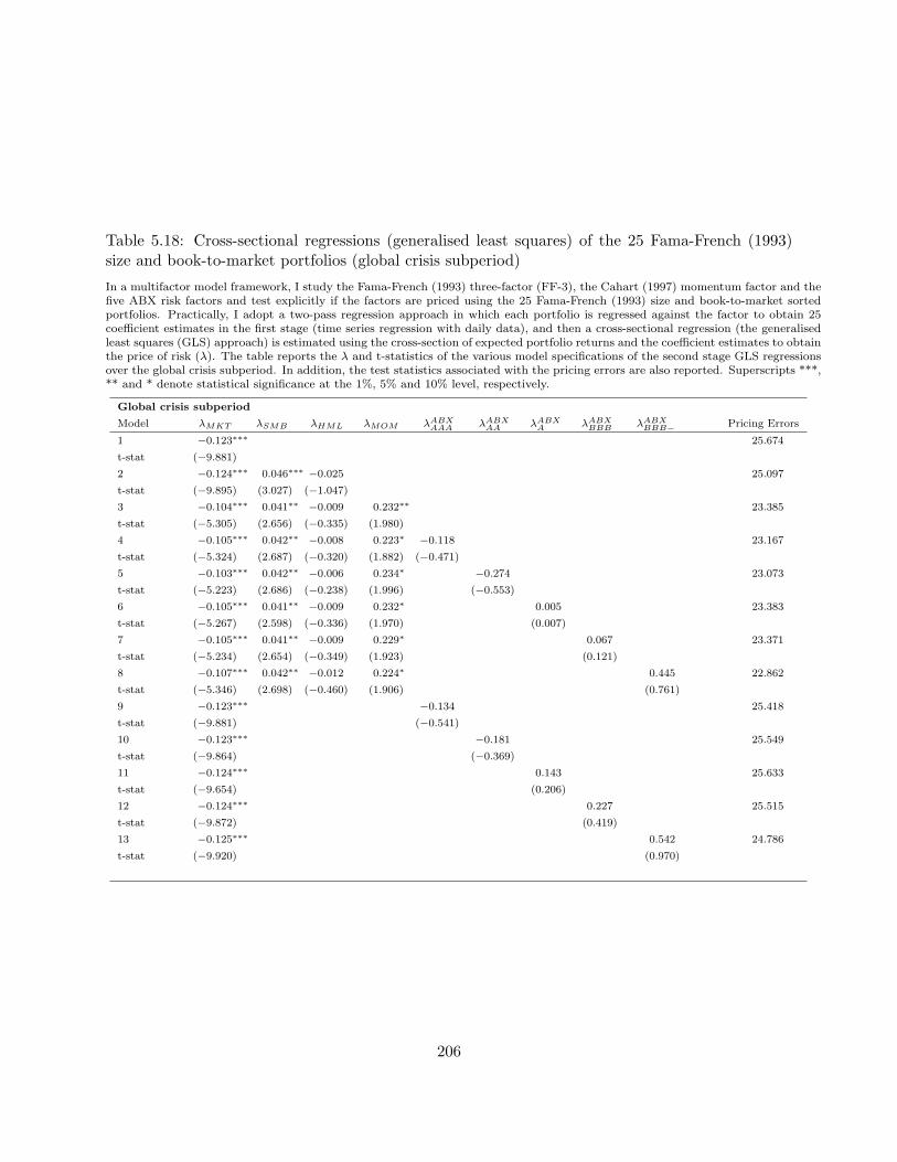
Table 5.18: Cross-sectional regressions (generalised least squares) of the 25 Fama-French (1993)size and book-to-market portfolios (global crisis subperiod)
In a multifactor model framework, I study the Fama-French (1993) three-factor (FF-3), the Cahart (1997) momentum factor and thefive ABX risk factors and test explicitly if the factors are priced using the 25 Fama-French (1993) size and book-to-market sortedportfolios. Practically, I adopt a two-pass regression approach in which each portfolio is regressed against the factor to obtain 25coefficient estimates in the first stage (time series regression with daily data), and then a cross-sectional regression (the generalisedleast squares (GLS) approach) is estimated using the cross-section of expected portfolio returns and the coefficient estimates to obtainthe price of risk (λ). The table reports the λ and t-statistics of the various model specifications of the second stage GLS regressionsover the global crisis subperiod. In addition, the test statistics associated with the pricing errors are also reported. Superscripts ***,** and * denote statistical significance at the 1%, 5% and 10% level, respectively.
Global crisis subperiod
Model λMKT λSMB λHML λMOM λABXAAA λABX
AA λABXA λABX
BBB λABXBBB− Pricing Errors
1 −0.123∗∗∗ 25.674
t-stat (−9.881)
2 −0.124∗∗∗ 0.046∗∗∗ −0.025 25.097
t-stat (−9.895) (3.027) (−1.047)
3 −0.104∗∗∗ 0.041∗∗ −0.009 0.232∗∗ 23.385
t-stat (−5.305) (2.656) (−0.335) (1.980)
4 −0.105∗∗∗ 0.042∗∗ −0.008 0.223∗ −0.118 23.167
t-stat (−5.324) (2.687) (−0.320) (1.882) (−0.471)
5 −0.103∗∗∗ 0.042∗∗ −0.006 0.234∗ −0.274 23.073
t-stat (−5.223) (2.686) (−0.238) (1.996) (−0.553)
6 −0.105∗∗∗ 0.041∗∗ −0.009 0.232∗ 0.005 23.383
t-stat (−5.267) (2.598) (−0.336) (1.970) (0.007)
7 −0.105∗∗∗ 0.041∗∗ −0.009 0.229∗ 0.067 23.371
t-stat (−5.234) (2.654) (−0.349) (1.923) (0.121)
8 −0.107∗∗∗ 0.042∗∗ −0.012 0.224∗ 0.445 22.862
t-stat (−5.346) (2.698) (−0.460) (1.906) (0.761)
9 −0.123∗∗∗ −0.134 25.418
t-stat (−9.881) (−0.541)
10 −0.123∗∗∗ −0.181 25.549
t-stat (−9.864) (−0.369)
11 −0.124∗∗∗ 0.143 25.633
t-stat (−9.654) (0.206)
12 −0.124∗∗∗ 0.227 25.515
t-stat (−9.872) (0.419)
13 −0.125∗∗∗ 0.542 24.786
t-stat (−9.920) (0.970)
206
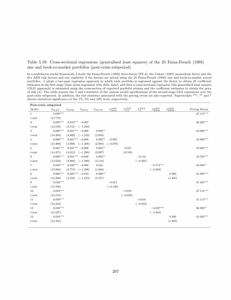
Table 5.19: Cross-sectional regressions (generalised least squares) of the 25 Fama-French (1993)size and book-to-market portfolios (post-crisis subperiod)
In a multifactor model framework, I study the Fama-French (1993) three-factor (FF-3), the Cahart (1997) momentum factor and thefive ABX risk factors and test explicitly if the factors are priced using the 25 Fama-French (1993) size and book-to-market sortedportfolios. I adopt a two-pass regression approach in which each portfolio is regressed against the factor to obtain 25 coefficientestimates in the first stage (time series regression with daily data), and then a cross-sectional regression (the generalised least squares(GLS) approach) is estimated using the cross-section of expected portfolio returns and the coefficient estimates to obtain the priceof risk (λ). The table reports the λ and t-statistics of the various model specifications of the second stage GLS regressions over thepost-crisis subperiod. In addition, the test statistics associated with the pricing errors are also reported. Superscripts ***, ** and *denote statistical significance at the 1%, 5% and 10% level, respectively.
Post-crisis subperiod
Model λMKT λSMB λHML λMOM λABXAAA λABX
AA λABXA λABX
BBB λABXBBB− Pricing Errors
1 0.059∗∗∗ 47.115∗∗∗
t-stat (14.772)
2 0.059∗∗∗ 0.019∗∗∗ −0.007 46.222∗∗∗
t-stat (14.559) (3.731) (−1.284)
3 0.060∗∗∗ 0.021∗∗∗ −0.008 0.082∗∗ 43.896∗∗∗
t-stat (14.494) (4.009) (−1.322) (2.094)
4 0.060∗∗∗ 0.021∗∗∗ −0.008 0.082∗∗ −0.007 43.890∗∗∗
t-stat (14.489) (4.008) (−1.308) (2.094) (−0.078)
5 0.061∗∗∗ 0.021∗∗∗ −0.008 0.082∗∗ 0.051 43.868∗∗∗
t-stat (14.471) (4.012) (−1.290) (2.097) (0.165)
6 0.060∗∗∗ 0.021∗∗∗ −0.008 0.083∗∗ −0.119 43.704∗∗∗
t-stat (14.033) (3.960) (−1.389) (2.116) (−0.405)
7 0.059∗∗∗ 0.020∗∗∗ −0.008 0.044 −0.774∗∗∗ 35.630∗∗
t-stat (13.904) (3.774) (−1.296) (1.060) (−2.962)
8 0.060∗∗∗ 0.023∗∗∗ −0.010 0.090∗∗ 0.380 41.895∗∗∗
t-stat (14.260) (4.234) (−1.672) (2.277) (1.465)
9 0.059∗∗∗ −0.011 47.105∗∗∗
t-stat (14.766) (−0.126)
10 0.059∗∗∗ −0.010 47.114∗∗∗
t-stat (14.744) (−0.033)
11 0.059∗∗∗ −0.010 47.113∗∗∗
t-stat (14.224) (−0.034)
12 0.058∗∗∗ −0.837∗∗∗ 36.298∗∗
t-stat (14.527) (−3.383)
13 0.058∗∗∗ 0.409 44.392∗∗∗
t-stat (14.455) (1.663)
207
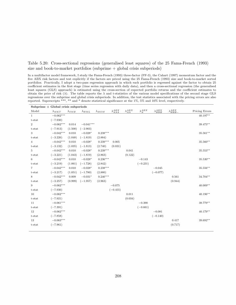
Table 5.20: Cross-sectional regressions (generalised least squares) of the 25 Fama-French (1993)size and book-to-market portfolios (subprime + global crisis subperiods)
In a multifactor model framework, I study the Fama-French (1993) three-factor (FF-3), the Cahart (1997) momentum factor and thefive ABX risk factors and test explicitly if the factors are priced using the 25 Fama-French (1993) size and book-to-market sortedportfolios. Practically, I adopt a two-pass regression approach in which each portfolio is regressed against the factor to obtain 25coefficient estimates in the first stage (time series regression with daily data), and then a cross-sectional regression (the generalisedleast squares (GLS) approach) is estimated using the cross-section of expected portfolio returns and the coefficient estimates toobtain the price of risk (λ). The table reports the λ and t-statistics of the various model specifications of the second stage GLSregressions over the subprime and global crisis subperiods. In addition, the test statistics associated with the pricing errors are alsoreported. Superscripts ***, ** and * denote statistical significance at the 1%, 5% and 10% level, respectively.
Subprime + Global crisis subperiods
Model λMKT λSMB λHML λMOM λABXAAA λABX
AA λABXA λABX
BBB λABXBBB− Pricing Errors
1 −0.062∗∗∗ 40.197∗∗
t-stat (−7.930)
2 −0.062∗∗∗ 0.014 −0.041∗∗∗ 39.473∗∗
t-stat (−7.913) (1.500) (−2.903)
3 −0.042∗∗∗ 0.010 −0.028∗ 0.238∗∗∗ 35.561∗∗
t-stat (−3.226) (1.048) (−1.819) (2.884)
4 −0.042∗∗∗ 0.010 −0.028∗ 0.239∗∗∗ 0.005 35.560∗∗
t-stat (−3.132) (1.035) (−1.813) (2.740) (0.031)
5 −0.042∗∗∗ 0.010 −0.028∗ 0.239∗∗∗ 0.041 35.553∗∗
t-stat (−3.221) (1.043) (−1.819) (2.863) (0.122)
6 −0.042∗∗∗ 0.010 −0.028∗ 0.236∗∗∗ −0.143 35.530∗∗
t-stat (−3.219) (1.061) (−1.728) (2.842) (−0.231)
7 −0.042∗∗∗ 0.010 −0.028∗ 0.238∗∗∗ −0.045 35.556∗∗
t-stat (−3.217) (1.051) (−1.780) (2.880) (−0.077)
8 −0.042∗∗∗ 0.009 −0.031∗ 0.246∗∗∗ 0.561 34.704∗∗
t-stat (−3.257) (0.999) (−1.957) (2.963) (0.944)
9 −0.062∗∗∗ −0.075 40.009∗∗
t-stat (−7.930) (−0.455)
10 −0.062∗∗∗ 0.011 40.196∗∗
t-stat (−7.921) (0.034)
11 −0.061∗∗∗ −0.390 39.779∗∗
t-stat (−7.391) (−0.661)
12 −0.062∗∗∗ −0.081 40.179∗∗
t-stat (−7.858) (−0.140)
13 −0.063∗∗∗ 0.417 39.692∗∗
t-stat (−7.961) (0.717)
208

Tab
le5.21
:Decileportfoliossorted
byABX
AAA
factorloadings(M
odel
1usingunorthogonalisedABX
index
returns)
This
table
reportsth
eeq
uallyweightedaveragesu
mmary
statisticsofth
edecileportfoliossorted
byth
eABX
factorloadingsestimatedusingth
etimeseries
regressionsas
shownin
Equation5.22(M
odel
1)andth
eunorthogonalised
ABX
index
retu
rns.
Allavailable
stock
sfrom
themajorUSex
changes
havebeenincluded
withatimeseries
regression
run
atth
een
dofea
chtradingmonth
forea
chstock
(Iscreen
outstock
swith
less
than
15dailyobservationsin
anymonth
s)to
obtain
time-varyingmonth
lyestimatesofth
efactorloadings.
Thefactors
inth
eregressionincludeth
elagged
excess
retu
rnsofth
eCRSP
value-weightedmarket
index
andan
unorthogonalized
ABX
factor.
Isort
thestock
sinto
decileportfoliosbasedonth
esu
mofABX
factorloadingsatth
een
dofea
chmonth
andreport
theeq
uallyweightedaveragesu
mmary
statistics
forth
edecileportfolios.
Portfolios1and10co
ntain
stock
swithth
elowestandhighestABX
factorloadingsresp
ectively.
Themarket
capitalisation,tu
rnover
ratios,
month
tand
t+
1retu
rns,
standard
dev
iations,
idiosyncraticvolatilities
(based
on
dailyobservations),averageα,su
mofmarket
betas(∑ 3 j
=1βj),
and
thesu
mofABX
factor
loadings(∑ 3 j
=1γj)ofea
chportfolioare
reported
.Ialsoreport
thesu
mmary
statisticsgrouped
bycrisis
subperiods.
Thefindingsare
basedonth
eABX
AAA
index
.
ABX
AA
AFactor
loadin
gs
βA
BX
Mark
etcapitalisa
tion
βA
BX
Equally
weighte
dm
onth
t+1
retu
rns
βA
BX
Avera
geα
Portfolio
full
pre
subprim
eglobal
post
Portfolio
full
pre
subprim
eglobal
post
Portfolio
full
pre
subprim
eglobal
post
11,172,637
1,328,452
1,478,530
1,326,684
1,011,718
10.27
0.39
-1.49
-1.97
0.58
10.35
0.29
-0.08
-0.06
0.66
22,677,012
2,888,933
2,914,949
2,397,921
2,797,302
20.42
0.68
-1.07
-2.12
1.10
20.08
0.08
-0.09
-0.05
0.19
33,448,176
3,847,746
3,635,659
2,772,545
3,727,678
30.33
0.77
-1.10
-2.27
1.11
30.04
0.04
-0.06
-0.01
0.10
43,323,210
3,364,426
3,836,093
2,645,978
3,499,561
40.40
0.66
-0.64
-1.95
1.00
40.03
0.01
-0.05
0.03
0.06
53,140,813
3,398,082
3,534,250
2,634,810
3,209,142
50.31
0.68
-0.74
-1.88
0.95
50.02
-0.01
-0.02
0.06
0.02
63,175,955
3,320,140
3,591,396
2,770,040
3,279,954
60.18
0.78
-0.76
-2.21
0.74
60.00
-0.02
-0.02
0.06
-0.01
73,414,452
3,158,787
4,350,498
2,888,631
3,498,673
70.13
0.83
-1.14
-2.13
0.66
7-0
.02
-0.05
-0.03
0.10
-0.05
83,153,435
3,065,314
3,849,403
2,677,599
3,259,054
80.18
0.97
-1.33
-2.04
0.66
8-0
.04
-0.09
-0.03
0.16
-0.11
92,423,820
2,627,505
2,657,343
2,342,748
2,406,900
90.16
0.83
-1.40
-2.51
0.71
9-0
.09
-0.17
-0.03
0.23
-0.22
10
1,076,864
1,388,836
1,164,774
1,088,878
1,019,046
10
-0.05
0.27
-1.80
-2.03
-0.04
10
-0.11
-0.29
0.09
0.64
-0.49
βA
BX
Turn
overra
tio
βA
BX
Avera
gestandard
deviations
βA
BX
Avera
gesu
mofm
ark
etbeta
s
Portfolio
full
pre
subprim
eglobal
post
Portfolio
full
pre
subprim
eglobal
post
Portfolio
full
pre
subprim
eglobal
post
12.66
2.24
2.41
2.79
2.89
15.08
3.72
3.91
7.48
4.45
12.45
1.02
2.67
3.39
2.33
22.85
1.68
2.06
3.08
3.52
23.15
2.26
2.46
4.73
2.75
21.59
1.12
1.70
1.94
1.48
32.84
1.55
2.08
3.17
3.38
32.60
1.84
2.03
3.95
2.27
31.25
0.94
1.28
1.49
1.22
43.13
1.69
2.38
3.44
3.74
42.23
1.58
1.71
3.47
1.94
41.03
0.93
1.04
1.20
0.98
53.33
1.61
2.77
4.07
3.52
51.99
1.36
1.54
3.22
1.69
50.86
0.87
0.81
0.99
0.81
63.24
1.50
2.53
4.16
3.61
62.02
1.38
1.55
3.27
1.73
60.81
0.86
0.77
0.86
0.77
73.01
1.48
2.51
3.50
3.32
72.29
1.55
1.78
3.65
1.98
70.80
0.95
0.77
0.79
0.73
82.82
1.55
2.63
3.19
3.17
82.65
1.91
2.07
4.14
2.28
80.77
1.20
0.64
0.68
0.68
92.63
1.67
2.01
3.00
2.93
93.22
2.34
2.50
4.89
2.77
90.71
1.43
0.56
0.51
0.57
10
2.88
2.29
2.57
3.15
3.15
10
5.16
3.78
4.00
7.75
4.43
10
0.32
2.04
0.02
-0.32
0.07
βA
BX
Equally
weighte
dm
onth
tre
turn
sβA
BX
Avera
geid
iosy
ncra
ticvolatilities(d
aily)
βA
BX
Avera
gesu
mofABX
facto
rloadin
gs
Portfolio
full
pre
subprim
eglobal
post
Portfolio
full
pre
subprim
eglobal
post
Portfolio
full
pre
subprim
eglobal
post
11.41
1.43
0.17
-3.70
1.65
13.76
2.90
2.95
5.37
3.27
1-1
42.97
-774.63
-95.92
-7.66
-12.20
2-0
.01
0.55
-0.75
-3.74
0.43
22.19
1.73
1.80
3.19
1.83
2-5
5.15
-297.58
-38.49
-3.13
-4.46
3-0
.08
0.46
-0.71
-3.64
0.51
31.73
1.40
1.46
2.57
1.43
3-2
9.99
-160.99
-21.76
-1.74
-2.40
40.02
0.54
-0.74
-3.19
0.74
41.45
1.19
1.20
2.20
1.17
4-1
4.80
-78.79
-11.31
-0.88
-1.17
50.04
0.48
-0.35
-3.03
0.68
51.25
1.01
1.05
1.99
0.98
5-4
.01
-20.46
-3.93
-0.22
-0.30
6-0
.03
0.42
-0.64
-3.67
0.93
61.28
1.04
1.05
2.01
1.02
65.63
32.34
2.03
0.39
0.46
7-0
.14
0.17
-0.82
-3.99
0.91
71.50
1.17
1.24
2.32
1.21
717.05
95.19
8.89
1.09
1.36
8-0
.20
0.36
-0.93
-4.29
0.87
81.79
1.46
1.47
2.71
1.45
833.18
183.93
18.70
2.02
2.62
9-0
.27
-0.16
-1.05
-4.22
0.67
92.25
1.79
1.83
3.34
1.86
959.93
330.90
35.13
3.46
4.75
10
1.54
1.08
-0.21
-3.72
2.30
10
3.84
2.92
3.03
5.69
3.24
10
150.98
823.67
96.44
8.35
12.59
209

Tab
le5.22
:Decileportfoliossorted
byABX
AA
factorloadings(M
odel
1usingunorthogonalisedABX
index
returns)
This
table
reportsth
eeq
uallyweightedaveragesu
mmary
statisticsofth
edecileportfoliossorted
byth
eABX
factorloadingsestimatedusingth
etimeseries
regressionsas
shownin
Equation5.22(M
odel
1)andth
eunorthogonalised
ABX
index
retu
rns.
Allavailable
stock
sfrom
themajorUSex
changes
havebeenincluded
withatimeseries
regressionru
natth
een
dofea
chtradingmonth
forea
chstock
(Iscreen
outstock
swithless
than15dailyobservationsin
anymonth
s)to
obtain
time-varyingmonth
lyestimatesofth
efactorloadings.
Thefactors
inth
eregressionincludeth
elagged
excess
retu
rnsofth
eCRSP
value-weightedmarket
index
andanunorthogonalized
ABX
factor.
Isort
thestock
sinto
decileportfoliosbasedonth
esu
mofABX
factorloadingsatth
een
dofea
chmonth
andreport
theeq
uallyweightedaveragesu
mmary
statistics
forth
edecileportfolios.
Portfolios1and10co
ntain
stock
swithth
elowestandhighestABX
factorloadingsresp
ectively.
Themarket
capitalisation,tu
rnover
ratios,
month
tandt+
1retu
rns,
standard
dev
iations,
idiosyncraticvolatilities
(basedondailyobservations),averageα,su
mofmarket
betas(∑ 3 j
=1βj),
andth
esu
mofABX
factor
loadings(∑ 3 j
=1γj)ofea
chportfolioare
reported
.Ialsoreport
thesu
mmary
statisticsgrouped
bycrisis
subperiods.
Thefindingsare
basedonth
eABX
AA
index
.
ABX
AA
Factor
loadin
gs
βA
BX
Mark
etcapitalisa
tion
βA
BX
Equally
weighte
dm
onth
t+1
retu
rns
βA
BX
Avera
geα
Portfolio
full
pre
subprim
eglobal
post
Portfolio
full
pre
subprim
eglobal
post
Portfolio
full
pre
subprim
eglobal
post
11,137,188
1,295,402
1,408,675
1,193,800
1,019,763
10.27
0.26
-1.77
-1.72
0.53
10.04
0.31
-0.37
-0.72
0.53
22,668,295
3,121,909
3,021,968
2,241,342
2,685,153
20.27
0.56
-1.45
-2.14
0.93
2-0
.02
0.08
-0.18
-0.31
0.16
33,398,695
3,393,549
3,763,562
2,970,391
3,572,511
30.21
0.64
-0.86
-2.41
0.93
3-0
.02
0.05
-0.12
-0.18
0.09
43,547,502
3,787,067
4,245,750
2,849,311
3,597,606
40.25
0.68
-0.64
-2.22
0.83
4-0
.01
0.02
-0.07
-0.09
0.05
53,161,214
3,098,740
3,502,100
2,767,313
3,370,199
50.26
0.76
-0.87
-1.95
0.85
50.00
0.00
-0.05
0.00
0.02
63,202,588
3,372,286
3,614,640
3,027,180
3,189,201
60.28
0.79
-0.86
-1.96
0.91
60.01
-0.03
-0.02
0.08
0.00
73,367,185
3,342,550
3,860,842
2,877,660
3,566,034
70.19
0.78
-1.03
-2.34
0.82
70.02
-0.05
0.01
0.18
-0.03
83,108,096
3,215,458
3,632,063
2,618,158
3,191,036
80.19
1.04
-1.27
-2.54
0.87
80.03
-0.09
0.03
0.31
-0.08
92,398,987
2,610,203
2,830,360
2,002,060
2,505,082
90.23
0.77
-1.36
-2.12
0.69
90.04
-0.17
0.09
0.49
-0.17
10
1,027,604
1,159,349
1,139,449
1,003,051
1,032,760
10
0.19
0.58
-1.36
-1.73
0.13
10
0.23
-0.31
0.38
1.31
-0.32
βA
BX
Turn
overra
tio
βA
BX
Avera
gestandard
deviations
βA
BX
Avera
gesu
mofm
ark
etbeta
s
Portfolio
full
pre
subprim
eglobal
post
Portfolio
full
pre
subprim
eglobal
post
Portfolio
full
pre
subprim
eglobal
post
12.72
2.23
2.47
2.68
3.06
15.08
3.72
3.92
7.53
4.46
12.88
2.61
3.09
3.37
2.41
22.70
1.68
1.90
3.13
3.03
23.13
2.22
2.43
4.73
2.76
21.70
1.61
1.71
1.94
1.53
32.93
1.53
2.03
3.11
3.69
32.59
1.81
2.03
3.99
2.27
31.30
1.19
1.35
1.45
1.20
43.14
1.52
2.62
3.89
3.46
42.24
1.55
1.71
3.50
1.95
41.05
1.01
1.05
1.15
1.00
53.37
1.59
2.53
4.19
3.81
51.98
1.36
1.53
3.17
1.71
50.88
0.87
0.88
0.98
0.82
63.27
1.59
2.72
3.88
3.69
62.02
1.39
1.55
3.28
1.70
60.79
0.82
0.78
0.91
0.72
73.04
1.54
2.41
3.94
3.27
72.29
1.57
1.79
3.66
1.94
70.76
0.81
0.75
0.84
0.71
82.87
1.56
2.67
3.34
3.17
82.67
1.88
2.12
4.16
2.27
80.70
0.83
0.68
0.75
0.65
92.60
1.72
2.06
2.75
2.97
93.22
2.37
2.48
4.88
2.77
90.56
0.89
0.50
0.44
0.57
10
2.76
2.32
2.55
2.68
3.10
10
5.17
3.87
4.00
7.66
4.46
10
-0.13
0.33
-0.25
-0.32
0.02
βA
BX
Equally
weighte
dm
onth
tre
turn
sβA
BX
Avera
geid
iosy
ncra
ticvolatilities(d
aily)
βA
BX
Avera
gesu
mofABX
facto
rloadin
gs
Portfolio
full
pre
subprim
eglobal
post
Portfolio
full
pre
subprim
eglobal
post
Portfolio
full
pre
subprim
eglobal
post
11.29
0.88
0.23
-3.85
1.76
13.78
2.92
2.94
5.48
3.27
1-4
7.77
-239.11
-50.37
-2.75
-3.76
2-0
.06
0.14
-0.71
-4.03
0.63
22.17
1.69
1.78
3.19
1.84
2-1
8.26
-92.09
-18.66
-1.08
-1.41
3-0
.06
0.33
-0.89
-3.68
0.72
31.74
1.37
1.46
2.60
1.44
3-1
0.01
-50.64
-10.07
-0.60
-0.77
4-0
.08
0.55
-0.70
-3.50
0.66
41.45
1.17
1.20
2.22
1.18
4-5
.09
-25.90
-5.03
-0.30
-0.39
5-0
.08
0.38
-0.74
-3.30
0.72
51.24
1.00
1.04
1.94
1.00
5-1
.59
-8.24
-1.45
-0.08
-0.11
60.00
0.42
-0.65
-3.27
0.77
61.27
1.04
1.05
2.00
0.99
61.54
7.57
1.70
0.13
0.12
7-0
.04
0.36
-0.62
-3.56
0.85
71.49
1.18
1.25
2.32
1.19
75.26
26.46
5.40
0.37
0.39
8-0
.09
0.45
-0.91
-3.88
0.75
81.79
1.43
1.51
2.72
1.44
810.49
53.20
10.40
0.69
0.78
9-0
.25
0.38
-0.96
-4.40
0.58
92.25
1.80
1.81
3.32
1.86
919.18
97.84
18.57
1.21
1.43
10
1.65
1.48
-0.06
-3.73
2.28
10
3.85
3.01
3.02
5.59
3.27
10
49.31
251.34
47.73
2.96
3.83
210

Tab
le5.23
:Decileportfoliossorted
byABX
Afactorloadings(M
odel
1usingunorthogonalisedABX
index
returns)
This
table
reportsth
eeq
uallyweightedaveragesu
mmary
statisticsofth
edecileportfoliossorted
byth
eABX
factorloadingsestimatedusingth
etimeseries
regressionsas
shownin
Equation5.22(M
odel
1)andth
eunorthogonalisedABX
index
retu
rns.
Allavailable
stock
sfrom
themajorUSex
changes
havebeenincluded
withatimeseries
regressionru
natth
een
dofea
chtradingmonth
forea
chstock
(Iscreen
outstock
swithless
than15dailyobservationsin
anymonth
s)to
obtain
time-varyingmonth
lyestimatesofth
efactorloadings.
Thefactors
inth
eregressionincludeth
elagged
excess
retu
rnsofth
eCRSP
value-weightedmarket
index
andanunorthogonalized
ABX
factor.
Isort
thestock
sinto
decileportfoliosbased
on
thesu
mofABX
factorloadingsatth
een
dofea
chmonth
and
report
theeq
uallyweighted
averagesu
mmary
statisticsforth
edecileportfolios.
Portfolios1and10co
ntain
stock
swithth
elowestandhighestABX
factorloadingsresp
ectively.
Themarket
capitalisation,tu
rnover
ratios,
month
tandt+
1retu
rns,
standard
dev
iations,
idiosyncraticvolatilities
(basedondailyobservations),averageα,su
mofmarket
betas(∑ 3 j
=1βj),
andth
esu
mof
ABX
factorloadings(∑ 3 j
=1γj)ofea
chportfolioare
reported
.Ialsoreport
thesu
mmary
statisticsgrouped
bycrisis
subperiods.
Thefindingsare
basedonth
eABX
Aindex
.
ABX
AFactor
loadin
gs
βA
BX
Mark
etcapitalisa
tion
βA
BX
Equally
weighte
dm
onth
t+1
retu
rns
βA
BX
Avera
geα
Portfolio
full
pre
subprim
eglobal
post
Portfolio
full
pre
subprim
eglobal
post
Portfolio
full
pre
subprim
eglobal
post
11,110,714
1,395,215
1,396,923
1,224,069
925,131
10.24
-0.14
-1.68
-1.20
0.32
1-0
.24
0.30
-0.44
-1.31
0.23
22,531,914
2,893,014
2,902,620
2,363,428
2,413,678
20.27
0.38
-1.09
-1.89
0.81
2-0
.12
0.09
-0.21
-0.52
0.05
33,292,835
3,251,317
4,062,675
2,820,937
3,282,228
30.26
0.65
-0.88
-2.49
0.93
3-0
.07
0.04
-0.14
-0.27
0.01
43,378,972
3,409,900
3,773,595
3,181,535
3,399,573
40.37
0.75
-0.78
-2.06
1.03
4-0
.03
0.01
-0.08
-0.12
0.01
53,288,339
3,541,488
3,366,087
2,993,522
3,453,324
50.26
0.67
-0.75
-2.09
0.89
50.00
-0.01
-0.04
0.01
0.01
63,164,633
3,081,826
3,486,597
2,764,551
3,343,468
60.16
0.70
-0.83
-2.27
0.78
60.03
-0.03
-0.01
0.13
0.01
73,303,129
3,400,288
4,281,180
2,703,080
3,352,566
70.17
0.95
-1.19
-2.54
0.88
70.06
-0.06
0.03
0.26
-0.01
83,200,454
3,195,333
3,610,004
2,479,959
3,569,077
80.27
1.05
-1.06
-2.09
0.80
80.09
-0.10
0.07
0.46
-0.03
92,563,606
2,643,570
2,995,033
1,914,893
2,812,226
90.31
0.94
-1.40
-2.10
0.84
90.15
-0.15
0.14
0.75
-0.07
10
1,179,787
1,573,689
1,143,734
1,098,503
1,176,303
10
0.01
0.93
-1.85
-2.37
0.21
10
0.54
-0.25
0.53
2.11
-0.10
βA
BX
Turn
overra
tio
βA
BX
Avera
gestandard
deviations
βA
BX
Avera
gesu
mofm
ark
etbeta
s
Portfolio
full
pre
subprim
eglobal
post
Portfolio
full
pre
subprim
eglobal
post
Portfolio
full
pre
subprim
eglobal
post
12.85
2.30
2.37
3.06
3.26
15.10
3.80
3.91
7.39
4.52
12.20
1.85
2.92
3.24
1.44
22.56
1.74
2.02
2.99
2.75
23.17
2.34
2.45
4.70
2.83
21.49
1.43
1.77
1.89
1.17
32.95
1.51
2.03
3.84
3.31
32.61
1.88
2.02
3.96
2.31
31.20
1.17
1.34
1.42
1.04
43.09
1.52
2.34
3.85
3.49
42.25
1.58
1.69
3.49
2.00
41.00
0.97
1.03
1.13
0.93
53.38
1.52
2.89
4.28
3.71
51.99
1.37
1.54
3.08
1.77
50.84
0.79
0.87
0.92
0.81
63.16
1.54
2.45
3.76
3.63
62.01
1.37
1.55
3.32
1.68
60.77
0.79
0.72
0.81
0.75
73.09
1.45
2.47
3.39
3.68
72.27
1.54
1.80
3.65
1.90
70.76
0.79
0.60
0.71
0.81
82.76
1.57
2.19
2.95
3.16
82.63
1.83
2.07
4.16
2.20
80.75
0.86
0.47
0.58
0.86
92.67
1.72
1.97
2.96
3.11
93.18
2.28
2.49
4.90
2.71
90.69
0.92
0.20
0.31
0.93
10
2.88
2.41
3.23
2.51
3.14
10
5.18
3.76
4.03
7.91
4.38
10
0.33
0.76
-0.78
-0.55
0.98
βA
BX
Equally
weighte
dm
onth
tre
turn
sβA
BX
Avera
geid
iosy
ncra
ticvolatilities(d
aily)
βA
BX
Avera
gesu
mofABX
facto
rloadin
gs
Portfolio
full
pre
subprim
eglobal
post
Portfolio
full
pre
subprim
eglobal
post
Portfolio
full
pre
subprim
eglobal
post
11.13
1.03
-0.15
-4.11
2.01
13.79
2.95
2.93
5.36
3.33
1-2
9.66
-161.46
-8.15
-2.55
-4.82
2-0
.04
0.57
-0.78
-3.80
0.69
22.21
1.79
1.79
3.17
1.92
2-1
1.49
-62.74
-3.20
-0.97
-1.86
3-0
.12
0.58
-0.92
-3.40
0.49
31.77
1.43
1.45
2.59
1.49
3-6
.32
-34.49
-1.82
-0.51
-1.04
4-0
.07
0.31
-0.68
-3.33
0.65
41.46
1.19
1.19
2.18
1.23
4-3
.13
-16.91
-0.98
-0.23
-0.54
50.00
0.30
-0.52
-3.17
0.77
51.25
1.02
1.06
1.88
1.04
5-0
.86
-4.51
-0.37
-0.02
-0.20
6-0
.08
0.28
-0.76
-3.55
0.83
61.27
1.02
1.05
2.04
0.99
61.01
5.72
0.14
0.18
0.09
7-0
.09
0.08
-0.72
-3.64
0.82
71.48
1.16
1.26
2.33
1.15
73.20
17.76
0.70
0.42
0.41
8-0
.12
0.09
-0.79
-4.05
0.77
81.77
1.39
1.48
2.74
1.41
86.28
34.66
1.49
0.74
0.85
9-0
.13
0.31
-0.89
-4.56
0.69
92.22
1.74
1.81
3.34
1.82
911.26
61.81
2.76
1.26
1.62
10
1.79
1.80
0.14
-3.59
2.01
10
3.87
2.92
3.06
5.82
3.22
10
28.91
156.88
7.49
3.14
4.56
211
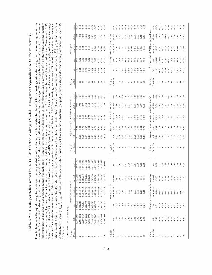
Tab
le5.24
:Decileportfoliossorted
byABX
BBB
factorloadings(M
odel
1usingunorthogonalisedABX
index
returns)
This
table
reportsth
eeq
uallyweightedaveragesu
mmary
statisticsofth
edecileportfoliossorted
byth
eABX
factorloadingsestimatedusingth
etimeseries
regressionsas
shownin
Equation5.22(M
odel
1)andth
eunorthogonalisedABX
index
retu
rns.
Allavailable
stock
sfrom
themajorUSex
changes
havebeenincluded
withatimeseries
regressionru
natth
een
dofea
chtradingmonth
forea
chstock
(Iscreen
outstock
swithless
than15dailyobservationsin
anymonth
s)to
obtain
time-varyingmonth
lyestimatesofth
efactorloadings.
Thefactors
inth
eregressionincludeth
elagged
excess
retu
rnsofth
eCRSP
value-weightedmarket
index
andanunorthogonalizedABX
factor.
Isort
thestock
sinto
decileportfoliosbased
on
thesu
mofABX
factorloadingsatth
een
dofea
chmonth
and
report
theeq
uallyweighted
averagesu
mmary
statisticsforth
edecileportfolios.
Portfolios1and10co
ntain
stock
swithth
elowestandhighestABX
factorloadingsresp
ectively.
Themarket
capitalisation,tu
rnover
ratios,
month
tandt+
1retu
rns,
standard
dev
iations,
idiosyncraticvolatilities
(basedondailyobservations),averageα,su
mofmarket
betas(∑ 3 j
=1βj),
andth
esu
m
ofABX
factorloadings(∑ 3 j
=1γj)ofea
chportfolioare
reported
.Ialsoreport
thesu
mmary
statisticsgrouped
bycrisis
subperiods.
Thefindingsare
basedonth
eABX
BBB
index
.
ABX
BBB
Factor
loadin
gs
βA
BX
Mark
etcapitalisa
tion
βA
BX
Equally
weighte
dm
onth
t+1
retu
rns
βA
BX
Avera
geα
Portfolio
full
pre
subprim
eglobal
post
Portfolio
full
pre
subprim
eglobal
post
Portfolio
full
pre
subprim
eglobal
post
11,053,296
1,204,632
1,191,640
1,032,135
1,002,579
1-0
.11
0.24
-1.85
-2.00
0.23
1-0
.19
0.09
-0.71
-1.39
0.46
22,551,902
2,882,671
2,831,357
2,134,054
2,631,806
20.29
0.63
-0.96
-1.70
0.81
2-0
.11
-0.02
-0.34
-0.52
0.13
33,297,047
3,715,134
3,307,913
2,814,043
3,508,099
30.25
0.75
-0.85
-1.97
0.88
3-0
.06
-0.02
-0.21
-0.28
0.09
43,437,202
3,324,867
3,827,774
2,861,480
3,665,441
40.23
0.57
-0.75
-2.15
0.94
4-0
.02
-0.02
-0.12
-0.09
0.04
53,319,374
3,411,491
3,615,320
3,001,634
3,338,887
50.14
0.84
-0.75
-2.46
0.92
50.00
-0.02
-0.06
0.02
0.01
63,195,027
3,389,318
3,435,074
2,746,283
3,311,962
60.15
0.87
-0.95
-2.10
0.86
60.03
-0.03
0.01
0.15
-0.01
73,494,787
3,399,035
4,259,559
2,961,761
3,579,689
70.10
0.76
-1.08
-2.12
0.80
70.05
-0.05
0.06
0.31
-0.05
83,259,371
3,165,559
4,204,585
2,642,384
3,283,942
80.14
0.91
-1.20
-2.12
0.87
80.08
-0.07
0.13
0.50
-0.10
92,476,485
2,585,077
3,074,271
2,224,207
2,424,959
90.24
0.90
-1.40
-2.17
0.97
90.13
-0.10
0.26
0.84
-0.20
10
1,100,205
1,295,960
1,272,243
1,130,359
979,687
10
-0.22
0.41
-1.71
-2.33
0.21
10
0.46
-0.14
0.78
2.31
-0.39
βA
BX
Turn
overra
tio
βA
BX
Avera
gestandard
deviations
βA
BX
Avera
gesu
mofm
ark
etbeta
s
Portfolio
full
pre
subprim
eglobal
post
Portfolio
full
pre
subprim
eglobal
post
Portfolio
full
pre
subprim
eglobal
post
12.67
2.35
2.49
2.61
2.93
15.02
3.77
3.99
7.39
4.40
11.63
2.14
2.76
2.13
0.74
22.49
1.66
2.07
2.67
2.87
23.08
2.27
2.49
4.64
2.68
21.27
1.65
1.68
1.50
0.86
32.77
1.59
2.14
3.18
3.21
32.54
1.83
2.07
3.94
2.19
31.06
1.22
1.35
1.23
0.79
42.90
1.46
2.22
3.87
3.17
42.23
1.58
1.76
3.52
1.91
40.93
0.99
1.04
1.05
0.79
53.35
1.63
2.58
4.34
3.69
51.99
1.35
1.55
3.24
1.71
50.83
0.83
0.87
0.88
0.76
63.38
1.56
2.61
3.90
3.93
62.00
1.38
1.54
3.23
1.73
60.78
0.82
0.69
0.81
0.78
73.05
1.51
2.39
3.63
3.54
72.26
1.56
1.73
3.61
1.99
70.84
0.88
0.64
0.84
0.89
82.98
1.56
2.07
3.04
3.86
82.63
1.89
2.03
4.09
2.33
80.92
0.91
0.57
0.83
1.08
92.73
1.69
2.28
3.03
3.13
93.21
2.34
2.43
4.97
2.83
90.97
0.87
0.38
0.77
1.29
10
2.93
2.25
3.11
3.30
2.93
10
5.14
3.78
3.96
7.92
4.51
10
1.08
0.99
-0.48
0.59
1.86
βA
BX
Equally
weighte
dm
onth
tre
turn
sβA
BX
Avera
geid
iosy
ncra
ticvolatilities(d
aily)
βA
BX
Avera
gesu
mofABX
facto
rloadin
gs
Portfolio
full
pre
subprim
eglobal
post
Portfolio
full
pre
subprim
eglobal
post
Portfolio
full
pre
subprim
eglobal
post
10.49
0.71
-0.58
-5.23
1.95
13.74
2.94
3.02
5.39
3.26
1-1
2.51
-43.58
-3.46
-5.30
-6.84
2-0
.48
0.18
-0.95
-4.61
0.67
22.16
1.74
1.84
3.17
1.81
2-4
.70
-16.46
-1.35
-2.07
-2.50
3-0
.33
0.20
-0.97
-3.93
0.95
31.71
1.38
1.49
2.58
1.40
3-2
.57
-8.91
-0.78
-1.19
-1.36
4-0
.23
0.36
-0.85
-3.24
0.79
41.45
1.19
1.24
2.22
1.17
4-1
.31
-4.45
-0.42
-0.64
-0.69
5-0
.24
0.42
-0.57
-3.21
0.70
51.25
1.00
1.07
1.99
0.99
5-0
.40
-1.21
-0.17
-0.22
-0.21
6-0
.14
0.34
-0.53
-3.14
0.80
61.26
1.03
1.04
1.99
1.01
60.41
1.65
0.04
0.16
0.21
7-0
.17
0.37
-0.59
-3.36
0.85
71.46
1.18
1.21
2.27
1.21
71.34
4.95
0.27
0.58
0.74
8-0
.25
0.42
-0.71
-3.50
0.66
81.77
1.44
1.45
2.68
1.49
82.66
9.64
0.59
1.16
1.48
9-0
.37
0.48
-0.65
-3.99
0.39
92.25
1.80
1.77
3.41
1.91
94.86
17.44
1.12
2.08
2.75
10
1.35
1.86
0.37
-2.99
1.95
10
3.84
2.96
3.03
5.82
3.30
10
12.77
44.63
3.02
5.42
7.40
212
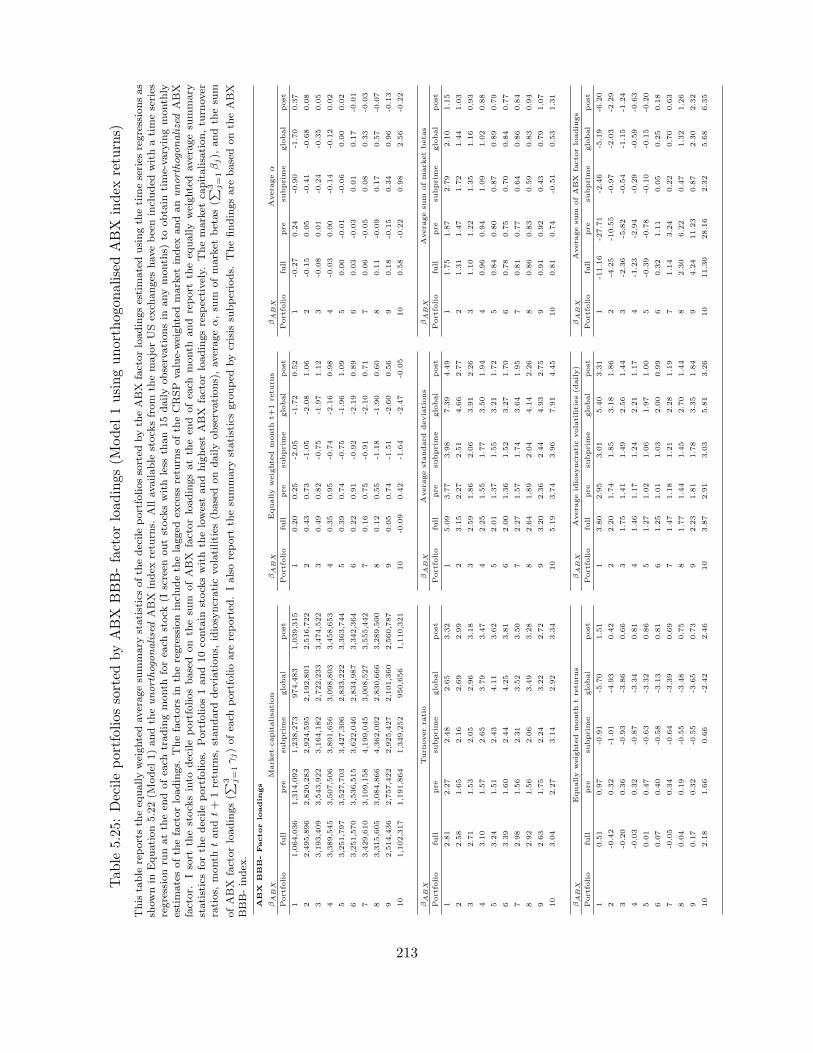
Tab
le5.25
:Decileportfoliossorted
byABX
BBB-factorloadings(M
odel
1usingunorthogonalisedABX
index
returns)
This
table
reportsth
eeq
uallyweightedaveragesu
mmary
statisticsofth
edecileportfoliossorted
byth
eABX
factorloadingsestimatedusingth
etimeseries
regressionsas
shownin
Equation5.22(M
odel
1)andth
eunorthogonalisedABX
index
retu
rns.
Allavailable
stock
sfrom
themajorUSex
changes
havebeenincluded
withatimeseries
regressionru
natth
een
dofea
chtradingmonth
forea
chstock
(Iscreen
outstock
swithless
than15dailyobservationsin
anymonth
s)to
obtain
time-varyingmonth
lyestimatesofth
efactorloadings.
Thefactors
inth
eregressionincludeth
elagged
excess
retu
rnsofth
eCRSP
value-weightedmarket
index
andanunorthogonalized
ABX
factor.
Isort
thestock
sinto
decileportfoliosbased
on
thesu
mofABX
factorloadingsatth
een
dofea
chmonth
and
report
theeq
uallyweighted
averagesu
mmary
statisticsforth
edecileportfolios.
Portfolios1and10co
ntain
stock
swithth
elowestandhighestABX
factorloadingsresp
ectively.
Themarket
capitalisation,tu
rnover
ratios,
month
tandt+
1retu
rns,
standard
dev
iations,
idiosyncraticvolatilities
(basedondailyobservations),averageα,su
mofmarket
betas(∑ 3 j
=1βj),
andth
esu
m
ofABX
factorloadings(∑ 3 j
=1γj)ofea
chportfolioare
reported
.Ialsoreport
thesu
mmary
statisticsgrouped
bycrisis
subperiods.
Thefindingsare
basedonth
eABX
BBB-index
.
ABX
BBB-Factor
loadin
gs
βA
BX
Mark
etcapitalisa
tion
βA
BX
Equally
weighte
dm
onth
t+1
retu
rns
βA
BX
Avera
geα
Portfolio
full
pre
subprim
eglobal
post
Portfolio
full
pre
subprim
eglobal
post
Portfolio
full
pre
subprim
eglobal
post
11,064,036
1,314,092
1,238,273
974,483
1,039,315
10.20
0.25
-2.05
-1.72
0.52
1-0
.27
0.24
-0.90
-1.70
0.37
22,495,896
2,820,283
2,924,595
2,192,801
2,516,722
20.43
0.73
-1.05
-2.08
1.06
2-0
.15
0.05
-0.41
-0.68
0.08
33,193,409
3,543,922
3,164,182
2,722,233
3,474,522
30.49
0.82
-0.75
-1.97
1.12
3-0
.08
0.01
-0.24
-0.35
0.05
43,389,545
3,507,506
3,801,656
3,098,803
3,458,653
40.35
0.95
-0.74
-2.16
0.98
4-0
.03
0.00
-0.14
-0.12
0.02
53,251,797
3,527,703
3,427,306
2,833,222
3,363,744
50.39
0.74
-0.75
-1.96
1.09
50.00
-0.01
-0.06
0.00
0.02
63,251,570
3,536,515
3,622,046
2,834,987
3,342,364
60.22
0.91
-0.92
-2.19
0.89
60.03
-0.03
0.01
0.17
-0.01
73,429,610
3,109,158
4,199,045
3,008,527
3,555,442
70.16
0.75
-0.91
-2.10
0.71
70.06
-0.05
0.08
0.33
-0.03
83,315,605
3,084,866
4,362,002
2,830,666
3,289,500
80.12
0.55
-1.18
-1.90
0.60
80.11
-0.09
0.17
0.57
-0.07
92,514,436
2,757,422
2,925,427
2,101,360
2,560,787
90.05
0.74
-1.51
-2.60
0.56
90.18
-0.15
0.34
0.96
-0.13
10
1,102,317
1,191,864
1,349,252
950,656
1,110,321
10
-0.09
0.42
-1.64
-2.47
-0.05
10
0.58
-0.22
0.98
2.56
-0.22
βA
BX
Turn
overra
tio
βA
BX
Avera
gestandard
deviations
βA
BX
Avera
gesu
mofm
ark
etbeta
s
Portfolio
full
pre
subprim
eglobal
post
Portfolio
full
pre
subprim
eglobal
post
Portfolio
full
pre
subprim
eglobal
post
12.81
2.27
2.48
2.65
3.32
15.09
3.77
3.98
7.39
4.49
11.75
1.87
2.79
2.10
1.15
22.58
1.65
2.16
2.69
2.99
23.15
2.27
2.51
4.66
2.77
21.31
1.47
1.72
1.44
1.03
32.71
1.53
2.05
2.96
3.18
32.59
1.86
2.06
3.91
2.26
31.10
1.22
1.35
1.16
0.93
43.10
1.57
2.65
3.79
3.47
42.25
1.55
1.77
3.50
1.94
40.96
0.94
1.09
1.02
0.88
53.24
1.51
2.43
4.11
3.62
52.01
1.37
1.55
3.21
1.72
50.84
0.80
0.87
0.89
0.79
63.39
1.60
2.44
4.25
3.81
62.00
1.36
1.52
3.27
1.70
60.78
0.75
0.70
0.84
0.77
72.98
1.56
2.31
3.52
3.50
72.27
1.57
1.74
3.64
1.95
70.81
0.77
0.64
0.86
0.84
82.92
1.56
2.06
3.49
3.28
82.64
1.89
2.04
4.14
2.26
80.86
0.83
0.59
0.83
0.94
92.63
1.75
2.24
3.22
2.72
93.20
2.36
2.44
4.93
2.75
90.91
0.92
0.43
0.79
1.07
10
3.04
2.27
3.14
2.92
3.34
10
5.19
3.74
3.96
7.91
4.45
10
0.81
0.74
-0.51
0.53
1.31
βA
BX
Equally
weighte
dm
onth
tre
turn
sβA
BX
Avera
geid
iosy
ncra
ticvolatilities(d
aily)
βA
BX
Avera
gesu
mofABX
facto
rloadin
gs
Portfolio
full
pre
subprim
eglobal
post
Portfolio
full
pre
subprim
eglobal
post
Portfolio
full
pre
subprim
eglobal
post
10.51
0.97
-0.91
-5.70
1.51
13.80
2.95
3.01
5.40
3.31
1-1
1.16
-27.71
-2.46
-5.19
-6.20
2-0
.42
0.32
-1.01
-4.93
0.42
22.20
1.74
1.85
3.18
1.86
2-4
.25
-10.55
-0.97
-2.03
-2.29
3-0
.20
0.36
-0.93
-3.86
0.66
31.75
1.41
1.49
2.56
1.44
3-2
.36
-5.82
-0.54
-1.15
-1.24
4-0
.03
0.32
-0.87
-3.34
0.81
41.46
1.17
1.24
2.21
1.17
4-1
.23
-2.94
-0.29
-0.59
-0.63
50.01
0.47
-0.63
-3.32
0.86
51.27
1.02
1.06
1.97
1.00
5-0
.39
-0.78
-0.10
-0.15
-0.20
60.07
0.40
-0.58
-3.13
0.81
61.25
1.01
1.03
2.00
0.99
60.32
1.11
0.05
0.25
0.18
7-0
.05
0.34
-0.64
-3.39
0.69
71.47
1.18
1.21
2.28
1.19
71.14
3.24
0.22
0.70
0.63
80.04
0.19
-0.55
-3.48
0.75
81.77
1.44
1.45
2.70
1.44
82.30
6.22
0.47
1.32
1.26
90.17
0.32
-0.55
-3.65
0.73
92.23
1.81
1.78
3.35
1.84
94.24
11.23
0.87
2.30
2.32
10
2.18
1.66
0.66
-2.42
2.46
10
3.87
2.91
3.03
5.81
3.26
10
11.30
28.16
2.32
5.68
6.35
213
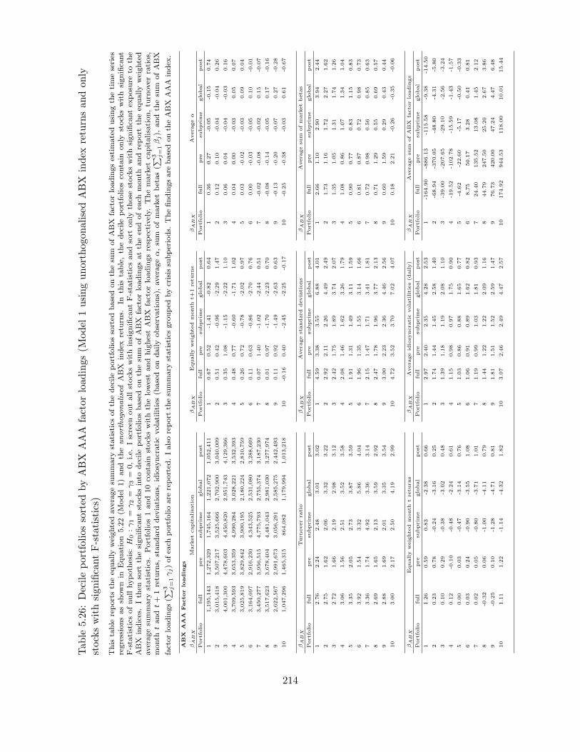
Tab
le5.26
:Decileportfoliossorted
byABX
AAA
factorloadings(M
odel
1usingunorthogonalisedABX
index
returnsan
don
lystockswithsign
ificantF-statistics)
This
table
reportsth
eeq
uallyweightedaveragesu
mmary
statisticsofth
edecileportfoliossorted
basedonth
esu
mofABX
factorloadingsestimatedusingth
etimeseries
regressionsassh
own
inEquation
5.22(M
odel
1)and
theunorthogonalised
ABX
index
retu
rns.
Inth
istable,th
edecileportfoliosco
ntain
only
stock
swith
significa
nt
F-statisticsofnullhypoth
esis:H
0:γ1=
γ2=
γ3=
0,i.e.
Iscreen
outallstock
swithinsignifica
ntF-statisticsandsort
only
those
stock
swithsignifica
ntex
posu
reto
the
ABX
indices.Ith
ensort
thesignifica
ntstock
sinto
decileportfoliosbasedonth
esu
mofABX
factorloadingsatth
een
dofea
chmonth
andreport
theeq
uallyweighted
averagesu
mmary
statistics.
Portfolios1and10co
ntain
stock
swithth
elowestandhighestABX
factorloadingsresp
ectively.
Themarket
capitalisation,tu
rnover
ratios,
month
tandt+
1retu
rns,
standard
dev
iations,
idiosyncraticvolatilities
(basedondailyobservations),averageα,su
mofmarket
betas(∑ 3 j
=1βj),
andth
esu
mofABX
factorloadings(∑ 3 j
=1γj)ofea
chportfolioare
reported
.Ialsoreport
thesu
mmary
statisticsgrouped
bycrisis
subperiods.
Thefindingsare
basedonth
eABX
AAA
index
.
ABX
AA
AFactor
loadin
gs
βA
BX
Mark
etcapitalisa
tion
βA
BX
Equally
weighte
dm
onth
t+1
retu
rns
βA
BX
Avera
geα
Portfolio
full
pre
subprim
eglobal
post
Portfolio
full
pre
subprim
eglobal
post
Portfolio
full
pre
subprim
eglobal
post
11,195,143
1,272,329
1,745,164
1,221,072
1,052,411
10.67
0.52
-1.41
-0.82
0.64
10.36
0.27
-0.05
-0.15
0.74
23,015,418
3,507,217
3,525,666
2,702,900
3,040,009
20.51
0.42
-0.96
-2.29
1.47
20.12
0.10
-0.04
-0.04
0.26
34,001,300
4,478,603
4,450,820
2,951,743
4,129,366
30.35
1.08
-1.15
-2.22
1.10
30.06
0.04
-0.04
-0.03
0.16
43,709,593
3,653,359
4,990,284
3,028,221
3,532,393
40.48
0.77
-0.60
-1.71
1.02
40.04
0.00
-0.03
0.05
0.07
53,025,819
3,829,842
3,900,195
2,180,224
2,810,759
50.26
0.72
-0.78
-2.02
0.97
50.03
-0.02
-0.03
0.09
0.04
63,164,097
2,916,230
4,343,525
2,531,080
3,288,669
60.11
0.63
-0.86
-2.70
0.76
60.00
-0.03
-0.05
0.10
-0.01
73,450,277
3,956,515
4,775,793
2,755,374
3,187,230
70.07
1.40
-1.02
-2.44
0.51
7-0
.02
-0.08
-0.02
0.15
-0.07
83,517,623
3,678,404
4,481,043
2,981,030
3,277,974
80.01
0.97
-1.70
-2.23
0.70
8-0
.08
-0.14
-0.05
0.17
-0.16
92,622,567
2,991,673
3,056,291
2,585,275
2,442,493
90.11
0.92
-1.49
-2.63
0.63
9-0
.13
-0.20
-0.07
0.27
-0.28
10
1,047,296
1,465,315
864,082
1,179,994
1,013,218
10
-0.16
0.40
-2.45
-2.25
-0.17
10
-0.25
-0.38
-0.03
0.61
-0.67
βA
BX
Turn
overra
tio
βA
BX
Avera
gestandard
deviations
βA
BX
Avera
gesu
mofm
ark
etbeta
s
Portfolio
full
pre
subprim
eglobal
post
Portfolio
full
pre
subprim
eglobal
post
Portfolio
full
pre
subprim
eglobal
post
12.76
2.24
2.48
3.01
3.02
14.59
3.38
3.55
6.88
4.01
12.66
1.10
2.90
3.94
2.44
22.75
1.62
2.06
3.32
3.22
22.92
2.11
2.26
4.49
2.49
21.73
1.16
1.72
2.27
1.62
32.72
1.66
2.19
2.98
3.12
32.42
1.75
1.89
3.74
2.07
31.35
1.05
1.31
1.74
1.26
43.06
1.56
2.51
3.52
3.58
42.08
1.46
1.62
3.26
1.79
41.08
0.86
1.07
1.34
1.04
53.35
2.05
2.73
3.87
3.59
51.91
1.31
1.49
3.11
1.59
50.90
0.77
0.83
1.15
0.83
63.92
1.54
3.32
5.86
4.04
61.96
1.35
1.55
3.14
1.66
60.81
0.87
0.72
0.98
0.73
73.36
1.74
4.92
3.36
3.14
72.15
1.47
1.71
3.41
1.81
70.72
0.98
0.56
0.85
0.63
82.69
1.65
2.13
3.59
2.92
82.47
1.78
1.96
3.77
2.13
80.71
1.29
0.55
0.69
0.57
92.88
1.69
2.01
3.35
3.54
93.00
2.23
2.36
4.46
2.56
90.60
1.59
0.29
0.43
0.44
10
3.00
2.17
2.50
4.19
2.99
10
4.72
3.52
3.70
7.02
4.07
10
0.18
2.21
-0.26
-0.35
-0.06
βA
BX
Equally
weighte
dm
onth
tre
turn
sβA
BX
Avera
geid
iosy
ncra
ticvolatilities(d
aily)
βA
BX
Avera
gesu
mofABX
facto
rloadin
gs
Portfolio
full
pre
subprim
eglobal
post
Portfolio
full
pre
subprim
eglobal
post
Portfolio
full
pre
subprim
eglobal
post
11.26
0.59
0.83
-2.38
0.66
12.97
2.40
2.35
4.28
2.53
1-1
64.90
-886.13
-115.58
-9.38
-14.50
20.23
0.78
-0.24
-3.16
0.25
21.74
1.44
1.45
2.58
1.40
2-6
8.94
-370.05
-48.80
-4.31
-5.80
30.10
0.29
-0.38
-3.02
0.48
31.39
1.18
1.19
2.08
1.10
3-3
9.00
-207.65
-29.10
-2.56
-3.24
40.12
-0.10
-0.48
-2.24
0.61
41.15
0.98
0.97
1.75
0.90
4-1
9.52
-102.78
-15.59
-1.43
-1.57
50.00
0.03
-0.47
-3.14
0.76
51.03
0.86
0.88
1.65
0.77
5-4
.62
-22.60
-5.17
-0.50
-0.33
60.03
0.24
-0.90
-3.55
1.08
61.06
0.91
0.89
1.62
0.82
68.75
50.17
3.28
0.41
0.81
70.02
0.05
-0.80
-3.71
1.01
71.19
0.99
1.03
1.81
0.93
724.40
135.52
13.08
1.45
2.12
8-0
.32
0.06
-1.00
-4.11
0.79
81.44
1.22
1.22
2.09
1.16
844.79
247.50
25.20
2.67
3.86
9-0
.25
0.10
-1.28
-4.71
0.81
91.81
1.51
1.52
2.59
1.47
976.73
420.00
47.24
4.47
6.48
10
1.11
1.22
-1.14
-4.32
1.82
10
3.07
2.46
2.49
4.47
2.57
10
174.92
944.53
118.00
10.01
15.44
214

Tab
le5.27
:Decileportfoliossorted
byABX
AA
factorloadings(M
odel
1usingunorthogonalisedABX
index
returnsan
don
lystockswithsign
ificantF-statistics)
This
table
reportsth
eeq
uallyweightedaveragesu
mmary
statisticsofth
edecileportfoliossorted
basedonth
esu
mofABX
factorloadingsestimatedusingth
etimeseries
regressionsassh
own
inEquation
5.22(M
odel
1)and
theunorthogonalised
ABX
index
retu
rns.
Inth
istable,th
edecileportfoliosco
ntain
only
stock
swith
significa
nt
F-statisticsofnullhypoth
esis:H
0:γ1=
γ2=
γ3=
0,i.e.
Iscreen
outallstock
swithinsignifica
ntF-statisticsandsort
only
those
stock
swithsignifica
ntex
posu
reto
the
ABX
index
.Ith
ensort
thesignifica
ntstock
sinto
decileportfoliosbasedonth
esu
mofABX
factorloadingsatth
een
dofea
chmonth
andreport
theeq
uallyweighted
averagesu
mmary
statistics.
Portfolios1and10co
ntain
stock
swithth
elowestandhighestABX
factorloadingsresp
ectively.
Themarket
capitalisation,tu
rnover
ratios,
month
tandt+
1retu
rns,
standard
dev
iations,
idiosyncraticvolatilities
(basedondailyobservations),averageα,su
mofmarket
betas(∑ 3 j
=1βj),
andth
esu
mofABX
factorloadings(∑ 3 j
=1γj)ofea
chportfolioare
reported
.Ialsoreport
thesu
mmary
statisticsgrouped
bycrisis
subperiods.
Thefindingsare
basedonth
eABX
AA
index
.
ABX
AA
Factor
loadin
gs
βA
BX
Mark
etcapitalisa
tion
βA
BX
Equally
weighte
dm
onth
t+1
retu
rns
βA
BX
Avera
geα
Portfolio
full
pre
subprim
eglobal
post
Portfolio
full
pre
subprim
eglobal
post
Portfolio
full
pre
subprim
eglobal
post
11,163,614
1,369,855
1,389,684
1,132,865
1,099,090
10.47
-0.14
-2.22
-1.05
0.81
1-0
.03
0.30
-0.44
-0.91
0.54
22,987,837
3,667,661
2,821,565
2,623,657
3,123,816
20.26
-0.14
-1.21
-1.59
0.68
2-0
.03
0.10
-0.20
-0.41
0.21
34,114,292
3,918,542
4,699,677
3,130,555
4,521,518
30.43
0.95
-0.77
-1.99
1.01
3-0
.02
0.08
-0.14
-0.22
0.12
43,767,968
3,837,531
4,975,303
2,926,966
3,692,850
40.16
1.14
-0.57
-3.21
0.94
40.01
0.06
-0.08
-0.09
0.09
53,073,229
3,215,295
4,074,405
2,634,431
3,029,132
50.43
0.91
-0.56
-1.80
0.90
50.02
0.00
-0.05
0.05
0.04
63,233,959
3,401,264
3,737,754
2,585,689
3,468,979
60.33
1.04
-0.74
-2.20
0.91
60.01
-0.05
-0.01
0.13
-0.01
73,662,827
3,735,980
4,895,037
2,756,292
3,585,057
70.21
0.91
-1.14
-2.16
0.99
70.02
-0.08
0.01
0.27
-0.06
83,389,073
4,117,790
3,877,832
2,942,618
3,321,344
80.24
1.60
-0.95
-3.11
0.95
80.04
-0.13
0.04
0.43
-0.10
92,656,262
2,837,330
2,890,901
2,343,379
2,827,588
90.39
0.65
-1.38
-0.80
0.47
90.05
-0.24
0.12
0.66
-0.21
10
1,020,168
1,239,308
981,359
1,156,758
987,955
10
0.10
0.93
-1.04
-1.95
-0.06
10
0.18
-0.41
0.31
1.49
-0.45
βA
BX
Turn
overra
tio
βA
BX
Avera
gestandard
deviations
βA
BX
Avera
gesu
mofm
ark
etbeta
s
Portfolio
full
pre
subprim
eglobal
post
Portfolio
full
pre
subprim
eglobal
post
Portfolio
full
pre
subprim
eglobal
post
12.72
1.99
2.47
2.84
3.05
14.58
3.27
3.67
6.75
4.07
13.17
2.83
3.44
3.78
2.64
22.88
1.86
2.21
2.63
3.61
22.90
2.01
2.34
4.39
2.53
21.88
1.75
1.87
2.26
1.66
32.76
1.46
1.85
3.25
3.19
32.40
1.70
1.93
3.68
2.10
31.42
1.26
1.48
1.63
1.30
43.43
1.67
3.16
4.73
3.43
42.08
1.48
1.58
3.24
1.79
41.09
0.96
1.06
1.24
1.06
53.37
1.69
2.71
4.27
3.56
51.94
1.32
1.44
3.19
1.65
50.93
0.80
0.98
1.09
0.87
63.26
1.59
2.62
4.16
3.51
61.98
1.36
1.50
3.24
1.63
60.82
0.86
0.74
1.03
0.74
72.87
1.61
2.36
3.38
3.20
72.16
1.46
1.70
3.43
1.84
70.70
0.77
0.73
0.70
0.67
82.76
1.75
2.06
3.36
3.08
82.50
1.83
1.98
3.89
2.13
80.61
0.97
0.61
0.58
0.54
92.53
1.99
2.05
2.63
2.81
93.04
2.26
2.33
4.61
2.60
90.42
0.89
0.47
0.24
0.37
10
2.82
2.08
2.30
2.38
3.65
10
4.76
3.50
3.68
7.08
4.14
10
-0.23
0.34
-0.12
-0.55
-0.16
βA
BX
Equally
weighte
dm
onth
tre
turn
sβA
BX
Avera
geid
iosy
ncra
ticvolatilities(d
aily)
βA
BX
Avera
gesu
mofABX
facto
rloadin
gs
Portfolio
full
pre
subprim
eglobal
post
Portfolio
full
pre
subprim
eglobal
post
Portfolio
full
pre
subprim
eglobal
post
10.61
0.37
1.03
-3.62
0.02
12.97
2.28
2.44
4.23
2.60
1-5
6.16
-278.40
-61.49
-3.26
-4.47
2-0
.08
-0.08
-0.19
-3.73
0.41
21.73
1.35
1.52
2.53
1.44
2-2
3.73
-118.07
-25.63
-1.42
-1.85
30.05
0.30
-0.43
-3.02
0.45
31.38
1.11
1.22
2.04
1.14
3-1
3.66
-68.03
-14.73
-0.82
-1.06
40.26
0.58
-0.66
-2.74
1.07
41.15
0.97
0.98
1.73
0.92
4-7
.14
-35.42
-7.84
-0.43
-0.56
50.19
0.30
-0.61
-2.80
1.03
51.04
0.85
0.84
1.67
0.82
5-2
.09
-9.83
-2.77
-0.10
-0.18
6-0
.05
-0.14
-0.56
-3.64
1.05
61.08
0.88
0.89
1.70
0.82
62.48
13.09
1.90
0.23
0.17
70.05
0.12
-0.85
-3.22
1.03
71.20
0.96
1.03
1.83
0.96
77.59
38.78
7.09
0.58
0.57
8-0
.06
0.31
-1.08
-3.85
1.12
81.45
1.21
1.26
2.18
1.16
814.61
74.51
14.04
1.01
1.08
9-0
.02
-0.14
-0.78
-4.19
1.02
91.84
1.51
1.51
2.69
1.50
925.39
129.72
24.30
1.63
1.91
10
1.59
1.48
-0.96
-4.02
2.53
10
3.09
2.38
2.49
4.53
2.61
10
58.80
300.49
56.02
3.59
4.63
215
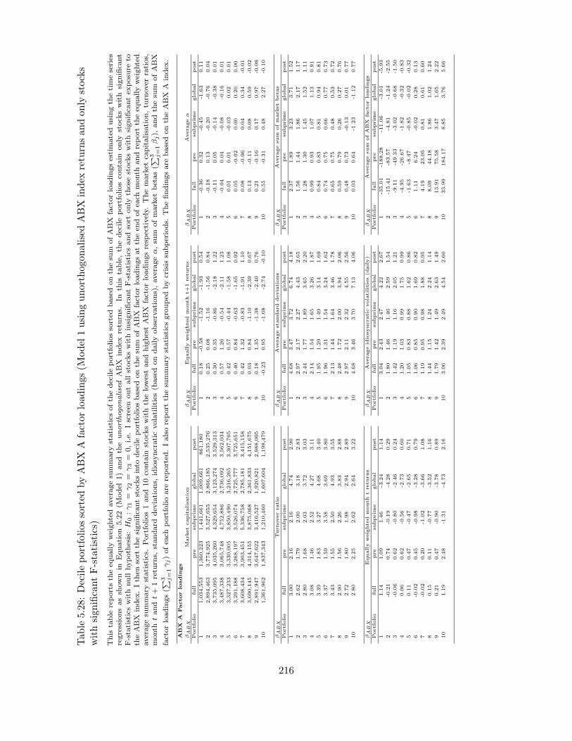
Tab
le5.28
:Decileportfoliossorted
byABX
Afactorloadings(M
odel
1usingunorthogonalisedABX
index
returnsandon
lystocks
withsign
ificantF-statistics)
This
table
reportsth
eeq
uallyweightedaveragesu
mmary
statisticsofth
edecileportfoliossorted
basedonth
esu
mofABX
factorloadingsestimatedusingth
etimeseries
regressionsassh
own
inEquation
5.22(M
odel
1)and
theunorthogonalised
ABX
index
retu
rns.
Inth
istable,th
edecileportfoliosco
ntain
only
stock
swith
significa
nt
F-statisticswithnullhypoth
esis:H
0:γ1=
γ2=
γ3=
0,i.e.
Iscreen
outallstock
swithinsignifica
ntF-statisticsandsort
only
those
stock
swithsignifica
ntex
posu
reto
theABX
index
.Ith
ensort
thesignifica
ntstock
sinto
decileportfoliosbasedonth
esu
mofABX
factorloadingsatth
een
dofea
chmonth
andreport
theeq
uallyweighted
averagesu
mmary
statistics.
Portfolios1and10co
ntain
stock
swithth
elowestandhighestABX
factorloadingsresp
ectively.
Themarket
capitalisation,tu
rnover
ratios,
month
tandt+
1retu
rns,
standard
dev
iations,
idiosyncraticvolatilities
(basedondailyobservations),averageα,su
mofmarket
betas(∑ 3 j
=1βj),
andth
esu
mofABX
factorloadings(∑ 3 j
=1γj)ofea
chportfolioare
reported
.Ialsoreport
thesu
mmary
statisticsgrouped
bycrisis
subperiods.
Thefindingsare
basedonth
eABX
Aindex
.
ABX
AFactor
loadin
gs
βA
BX
Mark
etcapitalisa
tion
βA
BX
Equally
weighte
dm
onth
t+1
retu
rns
βA
BX
Avera
geα
Portfolio
full
pre
subprim
eglobal
post
Portfolio
full
pre
subprim
eglobal
post
Portfolio
full
pre
subprim
eglobal
post
11,034,553
1,360,223
1,441,661
1,009,661
861,180
10.18
-0.58
-1.52
-1.93
0.54
1-0
.36
0.32
-0.45
-1.63
0.11
22,894,463
3,774,925
3,527,655
2,866,185
2,535,276
20.25
0.08
-1.16
-1.56
0.84
2-0
.18
0.13
-0.20
-0.76
0.04
33,735,095
4,035,260
4,329,654
3,123,274
3,529,313
30.30
0.35
-0.86
-2.18
1.22
3-0
.11
0.05
-0.14
-0.38
0.01
43,487,338
3,065,748
4,752,886
2,736,092
3,562,034
40.57
1.26
-0.54
-2.11
1.23
4-0
.04
0.04
-0.08
-0.16
0.01
53,327,233
3,330,005
3,850,490
3,216,265
3,307,765
50.42
0.57
-0.44
-1.58
1.08
50.01
0.01
-0.03
0.02
0.01
63,291,188
3,268,197
3,526,074
2,725,777
3,725,651
60.40
0.84
-0.63
-1.65
0.92
60.05
-0.02
0.00
0.20
0.00
73,608,434
3,903,451
5,336,758
2,785,181
3,415,158
70.42
1.32
-0.83
-1.91
1.10
70.08
-0.06
0.04
0.34
-0.01
83,690,145
4,314,155
3,875,068
2,361,833
4,151,675
80.03
0.84
-1.10
-2.39
0.67
80.13
-0.11
0.08
0.59
-0.02
92,891,947
3,647,622
3,416,527
1,920,821
2,988,005
90.18
1.35
-1.38
-2.40
0.76
90.21
-0.16
0.17
0.97
-0.08
10
1,361,962
1,837,343
1,210,460
1,607,604
1,198,479
10
-0.23
0.95
-1.68
-2.74
-0.10
10
0.55
-0.31
0.48
2.27
-0.10
βA
BX
Turn
overra
tio
βA
BX
Avera
gestandard
deviations
βA
BX
Avera
gesu
mofm
ark
etbeta
s
Portfolio
full
pre
subprim
eglobal
post
Portfolio
full
pre
subprim
eglobal
post
Portfolio
full
pre
subprim
eglobal
post
13.00
2.16
2.16
4.74
2.90
14.68
3.47
3.72
6.74
4.18
12.37
1.89
3.23
3.71
1.52
22.62
1.79
2.00
3.18
2.83
22.97
2.17
2.27
4.43
2.65
21.56
1.44
1.86
2.17
1.17
32.80
1.68
2.03
3.72
3.03
32.44
1.77
1.89
3.65
2.20
31.28
1.30
1.45
1.52
1.11
43.08
1.46
2.52
4.27
3.11
42.14
1.54
1.65
3.26
1.87
40.99
0.93
1.07
1.13
0.91
53.39
1.83
3.27
4.68
3.40
51.95
1.29
1.49
3.14
1.69
50.84
0.83
0.81
0.94
0.81
63.37
1.59
3.58
3.69
3.80
61.96
1.31
1.54
3.24
1.62
60.74
0.75
0.66
0.77
0.73
73.43
1.55
2.50
4.93
3.55
72.13
1.44
1.64
3.46
1.78
70.65
0.75
0.48
0.53
0.72
82.90
1.56
2.26
3.83
2.88
82.48
1.72
2.00
3.94
2.06
80.59
0.79
0.26
0.27
0.76
92.72
1.80
1.98
2.94
2.89
92.97
2.11
2.32
4.55
2.56
90.48
0.73
-0.13
0.01
0.77
10
2.80
2.25
2.62
2.64
3.22
10
4.68
3.46
3.70
7.13
4.06
10
0.03
0.64
-1.23
-1.12
0.77
βA
BX
Equally
weighte
dm
onth
tre
turn
sβA
BX
Avera
geid
iosy
ncra
ticvolatilities(d
aily)
βA
BX
Avera
gesu
mofABX
facto
rloadin
gs
Portfolio
full
pre
subprim
eglobal
post
Portfolio
full
pre
subprim
eglobal
post
Portfolio
full
pre
subprim
eglobal
post
11.14
1.09
1.46
-3.24
1.14
13.04
2.43
2.47
4.22
2.67
1-3
5.01
-188.28
-11.06
-3.01
-5.93
2-0
.21
0.74
-0.19
-4.28
0.29
21.80
1.46
1.46
2.59
1.54
2-1
5.41
-83.57
-4.81
-1.24
-2.55
3-0
.06
0.62
-0.80
-2.46
0.24
31.42
1.19
1.16
2.05
1.21
3-9
.11
-49.33
-3.02
-0.68
-1.50
40.06
0.62
-0.56
-2.73
0.60
41.20
1.03
0.99
1.75
0.99
4-4
.95
-26.67
-1.82
-0.32
-0.83
50.11
0.47
-0.47
-2.65
0.71
51.05
0.83
0.88
1.62
0.86
5-1
.63
-8.47
-0.85
-0.02
-0.32
6-0
.02
0.45
-0.98
-3.28
0.79
61.06
0.85
0.90
1.69
0.82
61.11
6.24
-0.02
0.28
0.13
7-0
.02
0.20
-1.02
-3.66
1.08
71.19
0.95
0.98
1.88
0.95
74.19
23.05
0.81
0.61
0.60
80.15
0.11
-0.77
-3.52
1.16
81.44
1.15
1.24
2.24
1.14
88.09
44.18
1.86
1.02
1.24
90.21
0.47
-0.90
-3.78
0.89
91.79
1.42
1.49
2.63
1.49
913.91
75.58
3.47
1.65
2.22
10
1.19
2.48
-1.31
-4.73
2.16
10
3.06
2.39
2.49
4.54
2.60
10
33.99
184.17
8.85
3.76
5.66
216
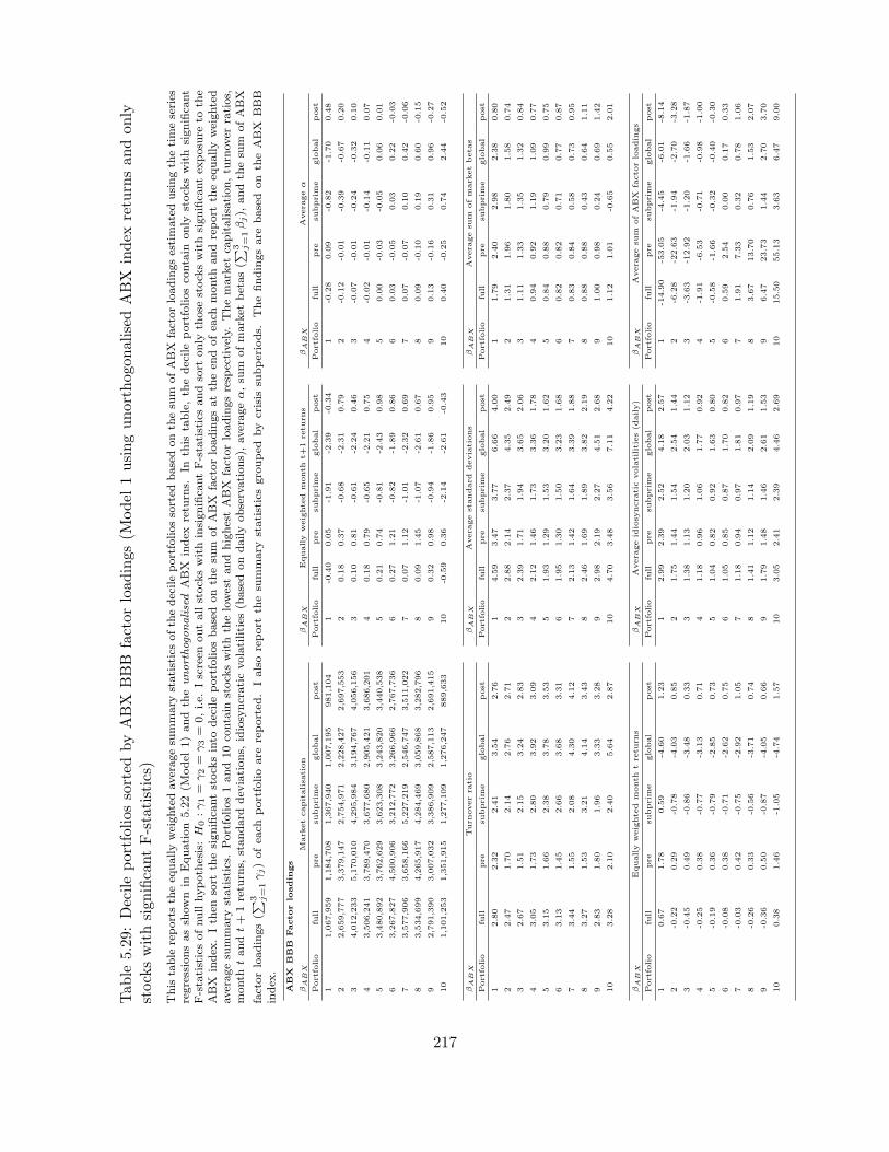
Tab
le5.29
:Decileportfoliossorted
byABX
BBB
factorloadings(M
odel
1usingunorthogonalisedABX
index
returnsan
don
lystockswithsign
ificantF-statistics)
This
table
reportsth
eeq
uallyweightedaveragesu
mmary
statisticsofth
edecileportfoliossorted
basedonth
esu
mofABX
factorloadingsestimatedusingth
etimeseries
regressionsassh
own
inEquation
5.22(M
odel
1)and
theunorthogonalised
ABX
index
retu
rns.
Inth
istable,th
edecileportfoliosco
ntain
only
stock
swith
significa
nt
F-statisticsofnullhypoth
esis:H
0:γ1=
γ2=
γ3=
0,i.e.
Iscreen
outallstock
swithinsignifica
ntF-statisticsandsort
only
those
stock
swithsignifica
ntex
posu
reto
the
ABX
index
.Ith
ensort
thesignifica
ntstock
sinto
decileportfoliosbasedonth
esu
mofABX
factorloadingsatth
een
dofea
chmonth
andreport
theeq
uallyweighted
averagesu
mmary
statistics.
Portfolios1and10co
ntain
stock
swithth
elowestandhighestABX
factorloadingsresp
ectively.
Themarket
capitalisation,tu
rnover
ratios,
month
tandt+
1retu
rns,
standard
dev
iations,
idiosyncraticvolatilities
(basedondailyobservations),averageα,su
mofmarket
betas(∑ 3 j
=1βj),
andth
esu
mofABX
factorloadings(∑ 3 j
=1γj)ofea
chportfolioare
reported
.Ialsoreport
thesu
mmary
statisticsgrouped
bycrisis
subperiods.
Thefindingsare
based
on
theABX
BBB
index
.
ABX
BBB
Factor
loadin
gs
βA
BX
Mark
etcapitalisa
tion
βA
BX
Equally
weighte
dm
onth
t+1
retu
rns
βA
BX
Avera
geα
Portfolio
full
pre
subprim
eglobal
post
Portfolio
full
pre
subprim
eglobal
post
Portfolio
full
pre
subprim
eglobal
post
11,067,959
1,184,708
1,367,940
1,007,195
981,104
1-0
.40
0.05
-1.91
-2.39
-0.34
1-0
.28
0.09
-0.82
-1.70
0.48
22,659,777
3,379,147
2,754,971
2,228,427
2,697,553
20.18
0.37
-0.68
-2.31
0.79
2-0
.12
-0.01
-0.39
-0.67
0.20
34,012,233
5,170,010
4,295,984
3,194,767
4,056,156
30.10
0.81
-0.61
-2.24
0.46
3-0
.07
-0.01
-0.24
-0.32
0.10
43,506,241
3,789,470
3,677,680
2,905,421
3,686,201
40.18
0.79
-0.65
-2.21
0.75
4-0
.02
-0.01
-0.14
-0.11
0.07
53,480,892
3,762,629
3,623,308
3,243,820
3,440,538
50.21
0.74
-0.81
-2.43
0.98
50.00
-0.03
-0.05
0.06
0.01
63,267,827
4,500,906
3,212,772
3,266,966
2,767,736
60.27
1.21
-0.82
-1.89
0.86
60.03
-0.05
0.03
0.22
-0.03
73,577,906
3,658,166
5,227,219
2,546,747
3,511,022
70.07
1.12
-1.01
-2.32
0.69
70.07
-0.07
0.10
0.42
-0.06
83,534,699
4,265,917
4,284,469
3,059,868
3,282,796
80.09
1.45
-1.07
-2.61
0.67
80.09
-0.10
0.19
0.60
-0.15
92,791,390
3,007,032
3,386,909
2,587,113
2,691,415
90.32
0.98
-0.94
-1.86
0.95
90.13
-0.16
0.31
0.96
-0.27
10
1,101,253
1,351,915
1,277,109
1,276,247
889,633
10
-0.59
0.36
-2.14
-2.61
-0.43
10
0.40
-0.25
0.74
2.44
-0.52
βA
BX
Turn
overra
tio
βA
BX
Avera
gestandard
deviations
βA
BX
Avera
gesu
mofm
ark
etbeta
s
Portfolio
full
pre
subprim
eglobal
post
Portfolio
full
pre
subprim
eglobal
post
Portfolio
full
pre
subprim
eglobal
post
12.80
2.32
2.41
3.54
2.76
14.59
3.47
3.77
6.66
4.00
11.79
2.40
2.98
2.38
0.80
22.47
1.70
2.14
2.76
2.71
22.88
2.14
2.37
4.35
2.49
21.31
1.96
1.80
1.58
0.74
32.67
1.51
2.15
3.24
2.83
32.39
1.71
1.94
3.65
2.06
31.11
1.33
1.35
1.32
0.84
43.05
1.73
2.80
3.92
3.09
42.12
1.46
1.73
3.36
1.78
40.94
0.92
1.19
1.09
0.77
53.15
1.66
2.38
3.78
3.53
51.93
1.29
1.53
3.20
1.62
50.84
0.88
0.79
0.99
0.75
63.13
1.45
2.66
3.68
3.31
61.95
1.30
1.50
3.23
1.68
60.82
0.82
0.71
0.77
0.87
73.44
1.55
2.08
4.30
4.12
72.13
1.42
1.64
3.39
1.88
70.83
0.84
0.58
0.73
0.95
83.27
1.53
3.21
4.14
3.43
82.46
1.69
1.89
3.82
2.19
80.88
0.88
0.43
0.64
1.11
92.83
1.80
1.96
3.33
3.28
92.98
2.19
2.27
4.51
2.68
91.00
0.98
0.24
0.69
1.42
10
3.28
2.10
2.40
5.64
2.87
10
4.70
3.48
3.56
7.11
4.22
10
1.12
1.01
-0.65
0.55
2.01
βA
BX
Equally
weighte
dm
onth
tre
turn
sβA
BX
Avera
geid
iosy
ncra
ticvolatilities(d
aily)
βA
BX
Avera
gesu
mofABX
facto
rloadin
gs
Portfolio
full
pre
subprim
eglobal
post
Portfolio
full
pre
subprim
eglobal
post
Portfolio
full
pre
subprim
eglobal
post
10.67
1.78
0.59
-4.60
1.23
12.99
2.39
2.52
4.18
2.57
1-1
4.90
-53.05
-4.45
-6.01
-8.14
2-0
.22
0.29
-0.78
-4.03
0.85
21.75
1.44
1.54
2.54
1.44
2-6
.28
-22.63
-1.94
-2.70
-3.28
3-0
.45
0.49
-0.86
-3.48
0.33
31.38
1.13
1.20
2.03
1.12
3-3
.63
-12.92
-1.20
-1.66
-1.87
4-0
.25
0.38
-0.77
-3.13
0.71
41.18
0.96
1.06
1.77
0.92
4-1
.91
-6.53
-0.71
-0.98
-1.00
5-0
.19
0.36
-0.79
-2.85
0.73
51.04
0.82
0.92
1.63
0.80
5-0
.58
-1.66
-0.32
-0.40
-0.30
6-0
.08
0.38
-0.71
-2.62
0.75
61.05
0.85
0.87
1.70
0.82
60.59
2.54
0.00
0.17
0.33
7-0
.03
0.42
-0.75
-2.92
1.05
71.18
0.94
0.97
1.81
0.97
71.91
7.33
0.32
0.78
1.06
8-0
.26
0.33
-0.56
-3.71
0.74
81.41
1.12
1.14
2.09
1.19
83.67
13.70
0.76
1.53
2.07
9-0
.36
0.50
-0.87
-4.05
0.66
91.79
1.48
1.46
2.61
1.53
96.47
23.73
1.44
2.70
3.70
10
0.38
1.46
-1.05
-4.74
1.57
10
3.05
2.41
2.39
4.46
2.69
10
15.50
55.13
3.63
6.47
9.00
217
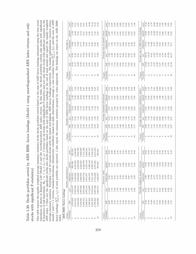
Tab
le5.30
:Decileportfoliossorted
byABX
BBB-factorloadings(M
odel
1usingunorthogonalisedABX
index
returnsan
don
lystockswithsign
ificantF-statistics)
This
table
reportsth
eeq
uallyweightedaveragesu
mmary
statisticsofth
edecileportfoliossorted
basedonth
esu
mofABX
factorloadingsestimatedusingth
etimeseries
regressionsassh
own
inEquation
5.22(M
odel
1)and
theunorthogonalised
ABX
index
retu
rns.
Inth
istable,th
edecileportfoliosco
ntain
only
stock
swith
significa
nt
F-statisticsofnullhypoth
esis:H
0:γ1=
γ2=
γ3=
0,i.e.
Iscreen
outallstock
swithinsignifica
ntF-statisticsandsort
only
those
stock
swithsignifica
ntex
posu
reto
the
ABX
index
.Ith
ensort
thesignifica
ntstock
sinto
decileportfoliosbasedonth
esu
mofABX
factorloadingsatth
een
dofea
chmonth
andreport
theeq
uallyweighted
averagesu
mmary
statistics.
Portfolios1and10co
ntain
stock
swithth
elowestandhighestABX
factorloadingsresp
ectively.
Themarket
capitalisation,tu
rnover
ratios,
month
tandt+
1retu
rns,
standard
dev
iations,
idiosyncraticvolatilities
(basedondailyobservations),averageα,su
mofmarket
betas(∑ 3 j
=1βj),
andth
esu
mofABX
factorloadings(∑ 3 j
=1γj)ofea
chportfolioare
reported
.Ialsoreport
thesu
mmary
statisticsgrouped
bycrisis
subperiods.
Thefindingsare
basedonth
eABX
BBB-
index
.
ABX
BBB-Factor
loadin
gs
βA
BX
Mark
etcapitalisa
tion
βA
BX
Equally
weighte
dm
onth
t+1
retu
rns
βA
BX
Avera
geα
Portfolio
full
pre
subprim
eglobal
post
Portfolio
full
pre
subprim
eglobal
post
Portfolio
full
pre
subprim
eglobal
post
11,073,632
1,214,477
1,563,974
925,368
997,525
10.45
0.44
-2.33
-1.46
0.77
1-0
.33
0.29
-0.96
-1.99
0.39
22,712,531
3,709,495
3,059,095
2,312,261
2,569,907
20.37
0.53
-0.82
-2.39
1.04
2-0
.17
0.10
-0.47
-0.85
0.13
33,654,032
4,330,415
3,833,026
2,923,088
3,903,706
30.59
1.14
-0.62
-2.06
1.24
3-0
.09
0.04
-0.29
-0.41
0.07
43,739,381
4,007,805
3,998,076
3,240,027
3,962,656
40.19
1.09
-1.10
-2.68
0.99
4-0
.03
0.01
-0.17
-0.15
0.05
53,084,474
3,031,869
3,900,740
2,462,678
3,131,338
50.35
1.03
-0.55
-2.20
0.87
5-0
.01
-0.02
-0.06
0.01
0.01
63,248,217
3,070,161
3,471,677
3,376,144
3,238,231
60.16
0.87
-0.96
-1.90
0.62
60.05
-0.04
0.05
0.24
-0.01
73,702,833
3,113,097
5,222,475
3,389,142
3,691,517
70.15
0.64
-0.87
-2.26
0.65
70.09
-0.07
0.13
0.48
-0.06
83,621,859
3,810,214
5,311,186
2,893,797
3,316,354
8-0
.18
0.55
-1.44
-2.43
0.26
80.13
-0.10
0.26
0.73
-0.12
92,758,955
2,997,384
3,176,629
2,257,961
2,815,233
90.04
1.24
-1.54
-2.76
0.45
90.20
-0.17
0.40
1.16
-0.19
10
1,034,689
1,055,371
1,426,537
965,991
938,216
10
-0.02
0.79
-1.27
-2.53
-0.01
10
0.53
-0.28
0.99
2.70
-0.35
βA
BX
Turn
overra
tio
βA
BX
Avera
gestandard
deviations
βA
BX
Avera
gesu
mofm
ark
etbeta
s
Portfolio
full
pre
subprim
eglobal
post
Portfolio
full
pre
subprim
eglobal
post
Portfolio
full
pre
subprim
eglobal
post
12.60
2.06
2.42
2.60
2.93
14.65
3.43
3.75
6.65
4.11
11.80
1.96
3.11
2.08
1.16
22.69
1.73
2.25
3.17
2.89
22.94
2.13
2.31
4.41
2.56
21.31
1.48
1.90
1.44
0.99
32.79
1.86
2.43
3.41
2.88
32.41
1.68
1.96
3.60
2.09
31.10
1.20
1.44
1.16
0.93
43.14
1.70
3.15
3.21
3.43
42.12
1.47
1.67
3.34
1.80
40.94
0.93
1.19
1.01
0.82
53.18
1.46
2.58
3.87
3.61
51.96
1.28
1.58
3.14
1.66
50.83
0.73
0.97
0.83
0.80
63.32
1.84
2.78
4.06
3.54
61.96
1.33
1.52
3.26
1.64
60.76
0.69
0.68
0.79
0.79
73.39
1.63
2.38
4.22
4.00
72.17
1.49
1.68
3.46
1.88
70.75
0.72
0.56
0.72
0.82
83.04
1.67
2.87
3.94
2.92
82.49
1.75
1.90
3.87
2.18
80.82
0.86
0.46
0.68
0.97
92.92
1.84
1.92
3.74
3.12
92.99
2.14
2.26
4.53
2.63
90.85
0.77
0.23
0.67
1.10
10
3.25
2.22
2.58
3.59
3.82
10
4.71
3.36
3.54
7.20
4.08
10
0.81
0.90
-0.70
0.35
1.36
βA
BX
Equally
weighte
dm
onth
tre
turn
sβA
BX
Avera
geid
iosy
ncra
ticvolatilities(d
aily)
βA
BX
Avera
gesu
mofABX
facto
rloadin
gs
Portfolio
full
pre
subprim
eglobal
post
Portfolio
full
pre
subprim
eglobal
post
Portfolio
full
pre
subprim
eglobal
post
10.42
0.72
1.80
-5.76
0.62
13.06
2.39
2.51
4.22
2.63
1-1
2.85
-33.70
-3.13
-6.08
-7.43
2-0
.55
0.53
-0.89
-4.92
0.02
21.79
1.43
1.49
2.58
1.47
2-5
.37
-14.37
-1.36
-2.62
-2.99
3-0
.20
0.25
-0.78
-3.49
0.54
31.41
1.10
1.23
2.03
1.14
3-3
.12
-8.31
-0.82
-1.53
-1.70
40.04
0.42
-0.71
-3.04
0.75
41.19
0.95
1.02
1.82
0.91
4-1
.67
-4.33
-0.47
-0.82
-0.88
5-0
.13
0.11
-0.73
-3.26
0.70
51.07
0.82
0.94
1.66
0.82
5-0
.56
-1.30
-0.20
-0.22
-0.26
60.08
0.31
-0.57
-3.06
0.92
61.06
0.85
0.90
1.68
0.82
60.47
1.63
0.05
0.34
0.32
70.03
0.38
-0.85
-2.52
0.58
71.21
0.98
1.01
1.86
0.97
71.60
4.78
0.30
0.96
1.00
80.06
0.69
-0.67
-3.24
0.76
81.43
1.15
1.17
2.13
1.17
83.10
8.92
0.63
1.73
1.88
90.06
0.22
-0.79
-3.48
0.77
91.81
1.45
1.44
2.63
1.51
95.44
15.30
1.14
2.86
3.25
10
1.73
2.45
-0.17
-3.00
2.18
10
3.07
2.31
2.38
4.54
2.60
10
13.15
34.17
2.71
6.53
7.93
218

Tab
le5.31
:Decileportfoliossorted
byABX
AAA
factorloadings(M
odel
2usingorthogonalisedABX
index
returns)
This
table
reportsth
eeq
uallyweighted
averagesu
mmary
statisticsofth
edecileportfoliossorted
byth
eABX
factorloadingsestimated
usingth
etimeseries
regression
assh
ownin
Equation5.23(M
odel
2)andth
eorthogonalised
ABX
innovations.
Allavailable
stock
sfrom
themajorUSex
changes
havebeenincluded
withatimeseries
regressionru
natth
een
dofea
chtradingmonth
forea
chstock
(Iscreen
outstock
swithless
than15dailyobservationsin
anymonth
s)to
obtain
time-varyingmonth
lyestimatesofth
efactorloadings.
Thefactors
inth
eregression
includeth
elagged
excess
retu
rnsofth
eCRSP
value-weighted
market
index
and
an
orthogonalised
ABX
factor.
Isort
thestock
sinto
decileportfoliosbasedonth
esu
mofABX
factorloadingsatth
een
dofea
chmonth
andreport
theeq
uallyweightedaveragesu
mmary
statistics
forth
edecileportfolios.
Portfolios1and10co
ntain
stock
swithth
elowestandhighestABX
factorloadingsresp
ectively.
Themarket
capitalisation,tu
rnover
ratios,
month
tandt+
1retu
rns,
standard
dev
iations,
idiosyncraticvolatilities
(basedondailyobservations),averageα,su
mofmarket
betas(∑ 3 j
=1βj),
andth
esu
mofABX
factor
loadings(∑ 3 j
=1γj)ofea
chportfolioare
reported
.Ialsoreport
thesu
mmary
statisticsgrouped
bycrisis
subperiods.
Thefindingsare
basedonth
eorthogonalisedABX
AAA
index
.
ABX
AA
AFactor
loadin
gs
βA
BX
Mark
etcapitalisa
tion
βA
BX
Equally
weighte
dm
onth
t+1
retu
rns
βA
BX
Avera
geα
Portfolio
full
pre
subprim
eglobal
post
Portfolio
full
pre
subprim
eglobal
post
Portfolio
full
pre
subprim
eglobal
post
11,102,660
1,139,443
1,398,455
1,195,477
1,013,886
10.26
0.55
-1.53
-2.06
0.54
10.42
-0.02
-0.07
0.02
0.91
22,763,735
3,224,598
3,225,689
2,357,187
2,782,846
20.47
0.84
-1.30
-1.97
1.17
20.11
-0.06
-0.08
0.00
0.28
33,424,733
3,706,232
3,656,993
2,708,421
3,763,202
30.40
0.90
-0.78
-2.29
1.11
30.06
-0.04
-0.05
0.01
0.15
43,341,220
3,322,777
3,631,383
2,722,172
3,592,997
40.41
0.81
-0.66
-2.02
1.00
40.04
-0.02
-0.04
0.04
0.08
53,115,173
2,896,602
3,648,092
2,698,599
3,276,383
50.27
0.74
-0.88
-1.98
0.93
50.02
-0.01
-0.03
0.06
0.03
63,172,544
3,265,419
3,802,291
2,779,229
3,171,514
60.16
0.56
-0.88
-2.24
0.82
60.00
-0.01
-0.03
0.07
-0.02
73,349,704
3,321,713
4,017,068
2,876,230
3,431,784
70.15
0.66
-1.01
-1.99
0.68
7-0
.02
-0.01
-0.03
0.09
-0.08
83,146,872
3,191,440
3,570,899
2,732,158
3,292,501
80.13
0.58
-1.22
-2.03
0.66
8-0
.05
-0.03
-0.03
0.13
-0.16
92,519,956
2,935,176
2,900,524
2,363,218
2,397,366
90.17
0.72
-1.29
-2.37
0.60
9-0
.11
-0.03
-0.03
0.18
-0.31
10
1,060,734
1,366,001
1,132,392
1,097,036
999,109
10
-0.08
0.52
-1.94
-2.19
-0.03
10
-0.18
0.03
0.09
0.55
-0.75
βA
BX
Turn
overra
tio
βA
BX
Avera
gestandard
deviations
βA
BX
Avera
gesu
mofm
ark
errisk
facto
rloadin
gs
Portfolio
full
pre
subprim
eglobal
post
Portfolio
full
pre
subprim
eglobal
post
Portfolio
full
pre
subprim
eglobal
post
12.67
2.30
2.43
2.71
2.93
15.08
3.74
3.91
7.47
4.44
10.10
-5.83
-1.40
2.28
1.52
22.78
1.59
2.05
2.98
3.44
23.15
2.23
2.46
4.78
2.74
20.66
-1.55
0.08
1.50
1.18
32.88
1.58
2.25
3.25
3.39
32.59
1.84
2.01
3.97
2.27
30.77
-0.46
0.42
1.26
1.05
43.06
1.46
2.14
3.65
3.59
42.22
1.50
1.70
3.50
1.94
40.76
0.05
0.59
1.08
0.90
53.46
1.52
2.94
4.06
3.84
51.99
1.34
1.54
3.22
1.71
50.77
0.55
0.70
0.93
0.79
63.15
1.54
2.38
3.91
3.52
62.03
1.40
1.58
3.26
1.74
60.88
1.01
0.90
0.93
0.78
72.99
1.56
2.54
3.55
3.26
72.29
1.60
1.81
3.61
1.97
71.03
1.65
1.20
0.92
0.80
82.85
1.63
2.62
3.16
3.17
82.66
1.92
2.07
4.14
2.28
81.25
2.56
1.53
0.93
0.85
92.66
1.78
2.00
3.10
3.00
93.20
2.35
2.49
4.88
2.77
91.60
4.00
2.09
0.97
0.87
10
2.88
2.30
2.61
3.15
3.13
10
5.16
3.82
4.00
7.73
4.45
10
2.71
9.02
4.09
0.83
0.92
βA
BX
Equally
weighte
dm
onth
tre
turn
sβA
BX
Avera
geid
iosy
ncra
ticvolatilities(d
aily)
βA
BX
Avera
gesu
mofABX
facto
rloadin
gs
Portfolio
full
pre
subprim
eglobal
post
Portfolio
full
pre
subprim
eglobal
post
Portfolio
full
pre
subprim
eglobal
post
11.53
1.74
0.04
-3.52
1.75
13.75
2.90
2.95
5.35
3.25
1-3
6.34
-131.76
-54.57
-7.90
-11.97
2-0
.01
0.47
-0.72
-3.71
0.39
22.19
1.69
1.80
3.23
1.82
2-1
4.04
-51.73
-20.77
-3.21
-4.36
3-0
.05
0.42
-0.69
-3.58
0.58
31.73
1.39
1.44
2.58
1.43
3-7
.74
-28.84
-11.30
-1.79
-2.33
4-0
.01
0.43
-0.69
-3.21
0.69
41.45
1.13
1.19
2.23
1.18
4-3
.92
-14.94
-5.53
-0.91
-1.14
50.00
0.40
-0.49
-3.08
0.68
51.25
0.99
1.04
1.99
0.99
5-1
.16
-4.99
-1.32
-0.24
-0.28
6-0
.04
0.31
-0.67
-3.56
0.91
61.29
1.04
1.07
2.02
1.03
61.32
3.89
2.61
0.39
0.48
7-0
.10
0.39
-0.82
-3.87
0.94
71.49
1.21
1.26
2.29
1.21
74.18
14.23
6.96
1.08
1.37
8-0
.19
0.20
-0.87
-4.21
0.90
81.79
1.46
1.47
2.72
1.45
88.16
28.59
13.03
2.02
2.63
9-0
.35
0.07
-1.01
-4.65
0.64
92.24
1.79
1.81
3.33
1.85
914.73
52.68
22.71
3.52
4.74
10
1.48
0.91
-0.12
-3.85
2.23
10
3.85
2.93
3.02
5.69
3.26
10
38.20
138.38
57.09
8.56
12.60
219

Tab
le5.32
:Decileportfoliossorted
byABX
AA
factorloadings(M
odel
2usingorthogonalisedABX
index
returns)
This
table
reportsth
eeq
uallyweightedaveragesu
mmary
statisticsofth
edecileportfoliossorted
byth
eABX
factorloadingsestimatedusingth
etimeseries
regression
assh
ownin
Equation5.23(M
odel
2)andth
eorthogonalised
ABX
innovations.
Allavailable
stock
sfrom
themajorUSex
changes
havebeenincluded
withatimeseries
regressionru
natth
een
dofea
chtradingmonth
forea
chstock
(Iscreen
outstock
swithless
than15dailyobservationsin
anymonth
s)to
obtain
time-varyingmonth
lyestimatesofth
efactorloadings.
Thefactors
inth
eregressionincludeth
elagged
excess
retu
rnsofth
eCRSP
value-weightedmarket
index
andanorthogonalised
ABX
factor.
Isort
thestock
sinto
decileportfoliosbased
on
thesu
mofABX
factorloadingsatth
een
dofea
chmonth
and
report
theeq
uallyweighted
averagesu
mmary
statisticsforth
edecileportfolios.
Portfolios1and10co
ntain
stock
swithth
elowestandhighestABX
factorloadingsresp
ectively.
Themarket
capitalisation,tu
rnover
ratios,
month
tandt+
1retu
rns,
standard
dev
iations,
idiosyncraticvolatilities
(basedondailyobservations),averageα,su
mofmarket
betas(∑ 3 j
=1βj),
andth
esu
m
ofABX
factorloadings(∑ 3 j
=1γj)ofea
chportfolioare
reported
.Ialsoreport
thesu
mmary
statisticsgrouped
by
crisis
subperiods.
Thefindingsare
based
on
the
orthogonalisedABX
AA
index
.
ABX
AA
Factor
loadin
gs
βA
BX
Mark
etcapitalisa
tion
βA
BX
Equally
weighte
dm
onth
t+1
retu
rns
βA
BX
Avera
geα
Portfolio
full
pre
subprim
eglobal
post
Portfolio
full
pre
subprim
eglobal
post
Portfolio
full
pre
subprim
eglobal
post
11,057,719
1,029,841
1,297,032
1,127,198
1,006,281
10.22
0.32
-2.06
-1.69
0.50
11.19
4.42
1.61
-0.54
0.87
22,540,137
2,499,817
2,936,008
2,101,298
2,710,168
20.35
0.71
-1.35
-2.10
0.99
20.42
1.75
0.55
-0.24
0.28
33,324,333
3,136,454
3,537,495
3,022,493
3,590,796
30.33
1.01
-0.86
-2.24
0.91
30.24
1.00
0.28
-0.13
0.16
43,426,931
3,580,990
4,028,515
2,731,488
3,507,210
40.28
0.94
-0.72
-2.18
0.85
40.13
0.53
0.13
-0.05
0.08
53,213,878
2,941,893
3,771,641
2,902,762
3,355,964
50.29
0.83
-0.76
-1.96
0.86
50.05
0.21
0.02
0.01
0.03
63,190,026
3,498,755
3,427,186
2,987,039
3,261,647
60.24
0.59
-0.93
-2.12
0.90
6-0
.01
-0.08
-0.06
0.08
-0.01
73,391,290
3,644,326
3,788,219
2,851,465
3,515,795
70.12
0.71
-0.96
-2.40
0.77
7-0
.08
-0.42
-0.18
0.16
-0.06
83,266,945
3,717,634
3,871,901
2,814,787
3,203,169
80.14
0.71
-1.27
-2.43
0.84
8-0
.19
-0.87
-0.34
0.27
-0.15
92,501,796
2,931,464
3,040,657
2,047,204
2,508,117
90.26
0.65
-1.12
-2.22
0.75
9-0
.37
-1.70
-0.59
0.44
-0.29
10
1,078,735
1,354,336
1,276,663
942,772
1,056,968
10
0.13
0.41
-1.45
-1.76
0.09
10
-0.89
-4.35
-1.43
1.11
-0.66
βA
BX
Turn
overra
tio
βA
BX
Avera
gestandard
deviations
βA
BX
Avera
gesu
mofm
ark
etrisk
facto
rs
Portfolio
full
pre
subprim
eglobal
post
Portfolio
full
pre
subprim
eglobal
post
Portfolio
full
pre
subprim
eglobal
post
12.68
2.20
2.43
2.60
3.06
15.09
3.72
3.94
7.55
4.47
10.03
-7.79
-1.44
2.63
1.73
22.65
1.57
1.93
3.07
2.98
23.14
2.27
2.44
4.74
2.75
20.60
-2.54
0.04
1.68
1.26
33.00
1.50
2.21
3.34
3.70
32.61
1.86
2.03
3.98
2.27
30.68
-1.13
0.37
1.33
1.06
43.01
1.48
2.31
3.65
3.40
42.25
1.60
1.73
3.49
1.96
40.74
-0.21
0.56
1.10
0.93
53.38
1.62
2.54
4.14
3.85
51.99
1.40
1.53
3.18
1.71
50.75
0.37
0.71
0.91
0.81
63.41
1.58
2.84
4.13
3.86
62.01
1.34
1.54
3.30
1.71
60.84
0.96
0.86
0.91
0.74
73.03
1.46
2.94
3.63
3.21
72.27
1.56
1.78
3.61
1.93
71.00
1.72
1.14
0.92
0.75
82.81
1.67
2.13
3.42
3.13
82.66
1.85
2.09
4.18
2.26
81.22
2.77
1.45
0.89
0.78
92.66
1.83
2.04
2.97
2.98
93.21
2.33
2.47
4.87
2.78
91.56
4.66
1.96
0.73
0.82
10
2.76
2.35
2.61
2.63
3.08
10
5.16
3.80
4.02
7.65
4.46
10
2.65
10.66
3.85
0.43
0.69
βA
BX
Equally
weighte
dm
onth
tre
turn
sβA
BX
Avera
geid
iosy
ncra
ticvolatilities(d
aily)
βA
BX
Avera
gesu
mofABX
facto
rloadin
gs
Portfolio
full
pre
subprim
eglobal
post
Portfolio
full
pre
subprim
eglobal
post
Portfolio
full
pre
subprim
eglobal
post
11.40
1.66
0.02
-3.77
1.80
13.78
2.89
2.95
5.49
3.28
1-1
8.17
-72.56
-27.81
-2.86
-3.73
2-0
.01
0.45
-0.93
-3.84
0.61
22.18
1.72
1.78
3.20
1.84
2-7
.16
-29.29
-10.49
-1.12
-1.40
3-0
.11
0.33
-1.07
-3.71
0.67
31.75
1.40
1.46
2.60
1.44
3-4
.07
-16.95
-5.82
-0.63
-0.77
4-0
.13
0.25
-0.88
-3.42
0.67
41.46
1.20
1.21
2.21
1.18
4-2
.18
-9.23
-3.04
-0.32
-0.39
5-0
.12
0.34
-0.71
-3.31
0.68
51.25
1.03
1.04
1.95
0.99
5-0
.81
-3.63
-1.04
-0.09
-0.12
6-0
.05
0.41
-0.64
-3.45
0.77
61.27
1.00
1.03
2.02
1.00
60.36
1.11
0.65
0.12
0.11
70.00
0.22
-0.72
-3.49
0.93
71.47
1.17
1.24
2.27
1.18
71.69
6.51
2.58
0.36
0.39
8-0
.07
0.56
-0.79
-3.84
0.72
81.79
1.41
1.48
2.74
1.43
83.57
14.18
5.27
0.69
0.77
9-0
.22
-0.06
-0.64
-4.28
0.59
92.25
1.79
1.80
3.33
1.86
96.70
27.05
9.64
1.22
1.42
10
1.57
1.14
0.32
-4.07
2.27
10
3.85
2.97
3.06
5.61
3.27
10
17.68
71.74
25.24
3.02
3.79
220
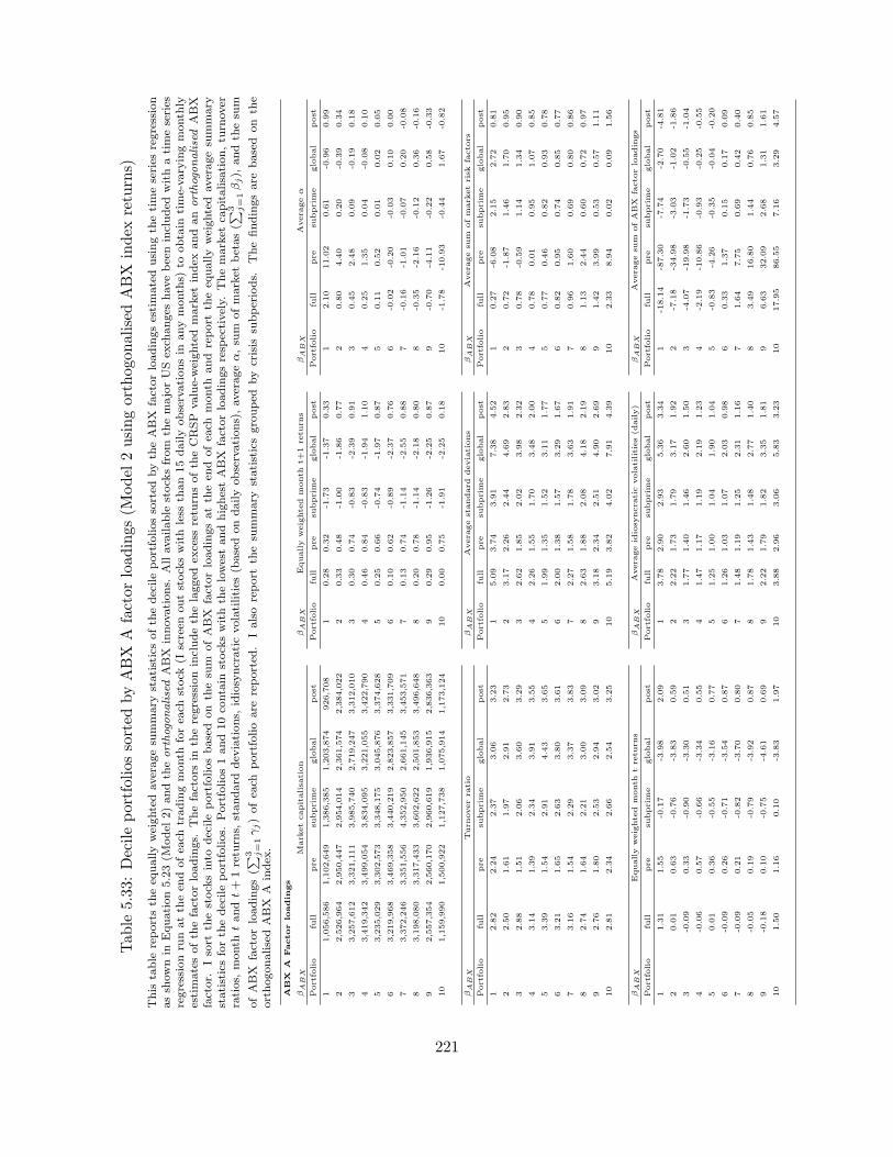
Tab
le5.33
:Decileportfoliossorted
byABX
Afactorloadings(M
odel
2usingorthogonalisedABX
index
returns)
This
table
reportsth
eeq
uallyweightedaveragesu
mmary
statisticsofth
edecileportfoliossorted
byth
eABX
factorloadingsestimatedusingth
etimeseries
regression
assh
ownin
Equation5.23(M
odel
2)andth
eorthogonalised
ABX
innovations.
Allavailable
stock
sfrom
themajorUSex
changes
havebeenincluded
withatimeseries
regressionru
natth
een
dofea
chtradingmonth
forea
chstock
(Iscreen
outstock
swithless
than15dailyobservationsin
anymonth
s)to
obtain
time-varyingmonth
lyestimatesofth
efactorloadings.
Thefactors
inth
eregressionincludeth
elagged
excess
retu
rnsofth
eCRSP
value-weightedmarket
index
andanorthogonalised
ABX
factor.
Isort
thestock
sinto
decileportfoliosbased
on
thesu
mofABX
factorloadingsatth
een
dofea
chmonth
and
report
theeq
uallyweighted
averagesu
mmary
statisticsforth
edecileportfolios.
Portfolios1and10co
ntain
stock
swithth
elowestandhighestABX
factorloadingsresp
ectively.
Themarket
capitalisation,tu
rnover
ratios,
month
tandt+
1retu
rns,
standard
dev
iations,
idiosyncraticvolatilities
(basedondailyobservations),averageα,su
mofmarket
betas(∑ 3 j
=1βj),
andth
esu
m
ofABX
factorloadings(∑ 3 j
=1γj)ofea
chportfolioare
reported
.Ialsoreport
thesu
mmary
statisticsgrouped
by
crisis
subperiods.
Thefindingsare
based
on
the
orthogonalisedABX
Aindex
.
ABX
AFactor
loadin
gs
βA
BX
Mark
etcapitalisa
tion
βA
BX
Equally
weighte
dm
onth
t+1
retu
rns
βA
BX
Avera
geα
Portfolio
full
pre
subprim
eglobal
post
Portfolio
full
pre
subprim
eglobal
post
Portfolio
full
pre
subprim
eglobal
post
11,056,586
1,102,649
1,386,385
1,203,874
926,708
10.28
0.32
-1.73
-1.37
0.33
12.10
11.02
0.61
-0.96
0.99
22,526,964
2,950,447
2,954,014
2,361,574
2,384,022
20.33
0.48
-1.00
-1.86
0.77
20.80
4.40
0.20
-0.39
0.34
33,257,612
3,321,111
3,985,740
2,719,247
3,312,010
30.30
0.74
-0.83
-2.39
0.91
30.45
2.48
0.09
-0.19
0.18
43,419,342
3,499,054
3,834,095
3,221,055
3,422,790
40.46
0.84
-0.83
-1.94
1.10
40.25
1.35
0.04
-0.08
0.10
53,235,029
3,302,573
3,348,175
3,045,876
3,374,628
50.25
0.66
-0.74
-1.97
0.87
50.11
0.52
0.01
0.02
0.05
63,219,968
3,469,358
3,440,219
2,823,857
3,331,709
60.10
0.62
-0.89
-2.37
0.76
6-0
.02
-0.20
-0.03
0.10
0.00
73,372,246
3,351,556
4,352,950
2,661,145
3,453,571
70.13
0.74
-1.14
-2.55
0.88
7-0
.16
-1.01
-0.07
0.20
-0.08
83,198,080
3,317,433
3,602,622
2,501,853
3,496,648
80.20
0.78
-1.14
-2.18
0.80
8-0
.35
-2.16
-0.12
0.36
-0.16
92,557,354
2,560,170
2,960,619
1,936,915
2,836,363
90.29
0.95
-1.26
-2.25
0.87
9-0
.70
-4.11
-0.22
0.58
-0.33
10
1,159,990
1,500,922
1,127,738
1,075,914
1,173,124
10
0.00
0.75
-1.91
-2.25
0.18
10
-1.78
-10.93
-0.44
1.67
-0.82
βA
BX
Turn
overra
tio
βA
BX
Avera
gestandard
deviations
βA
BX
Avera
gesu
mofm
ark
etrisk
facto
rs
Portfolio
full
pre
subprim
eglobal
post
Portfolio
full
pre
subprim
eglobal
post
Portfolio
full
pre
subprim
eglobal
post
12.82
2.24
2.37
3.06
3.23
15.09
3.74
3.91
7.38
4.52
10.27
-6.08
2.15
2.72
0.81
22.50
1.61
1.97
2.91
2.73
23.17
2.26
2.44
4.69
2.83
20.72
-1.87
1.46
1.70
0.95
32.88
1.51
2.06
3.60
3.29
32.62
1.85
2.02
3.98
2.32
30.78
-0.59
1.14
1.34
0.90
43.14
1.39
2.34
3.91
3.55
42.26
1.55
1.70
3.48
2.00
40.78
0.01
0.95
1.07
0.85
53.39
1.54
2.91
4.43
3.65
51.99
1.35
1.52
3.11
1.77
50.77
0.46
0.82
0.93
0.78
63.21
1.65
2.63
3.80
3.61
62.00
1.38
1.57
3.29
1.67
60.82
0.95
0.74
0.85
0.77
73.16
1.54
2.29
3.37
3.83
72.27
1.58
1.78
3.63
1.91
70.96
1.60
0.69
0.80
0.86
82.74
1.64
2.21
3.00
3.09
82.63
1.88
2.08
4.18
2.19
81.13
2.44
0.60
0.72
0.97
92.76
1.80
2.53
2.94
3.02
93.18
2.34
2.51
4.90
2.69
91.42
3.99
0.53
0.57
1.11
10
2.81
2.34
2.66
2.54
3.25
10
5.19
3.82
4.02
7.91
4.39
10
2.33
8.94
0.02
0.09
1.56
βA
BX
Equally
weighte
dm
onth
tre
turn
sβA
BX
Avera
geid
iosy
ncra
ticvolatilities(d
aily)
βA
BX
Avera
gesu
mofABX
facto
rloadin
gs
Portfolio
full
pre
subprim
eglobal
post
Portfolio
full
pre
subprim
eglobal
post
Portfolio
full
pre
subprim
eglobal
post
11.31
1.55
-0.17
-3.98
2.09
13.78
2.90
2.93
5.36
3.34
1-1
8.14
-87.30
-7.74
-2.70
-4.81
20.01
0.63
-0.76
-3.83
0.59
22.22
1.73
1.79
3.17
1.92
2-7
.18
-34.98
-3.03
-1.02
-1.86
3-0
.09
0.33
-0.90
-3.30
0.51
31.77
1.40
1.46
2.60
1.50
3-4
.07
-19.98
-1.73
-0.55
-1.04
4-0
.06
0.57
-0.66
-3.34
0.55
41.47
1.17
1.19
2.19
1.23
4-2
.19
-10.86
-0.93
-0.25
-0.55
50.01
0.36
-0.55
-3.16
0.77
51.25
1.00
1.04
1.90
1.04
5-0
.83
-4.26
-0.35
-0.04
-0.20
6-0
.09
0.26
-0.71
-3.54
0.87
61.26
1.03
1.07
2.03
0.98
60.33
1.37
0.15
0.17
0.09
7-0
.09
0.21
-0.82
-3.70
0.80
71.48
1.19
1.25
2.31
1.16
71.64
7.75
0.69
0.42
0.40
8-0
.05
0.19
-0.79
-3.92
0.87
81.78
1.43
1.48
2.77
1.40
83.49
16.80
1.44
0.76
0.85
9-0
.18
0.10
-0.75
-4.61
0.69
92.22
1.79
1.82
3.35
1.81
96.63
32.09
2.68
1.31
1.61
10
1.50
1.16
0.10
-3.83
1.97
10
3.88
2.96
3.06
5.83
3.23
10
17.95
86.55
7.16
3.29
4.57
221

Tab
le5.34
:Decileportfoliossorted
byABX
BBB
factorloadings(M
odel
2usingorthogonalisedABX
index
returns)
This
table
reportsth
eeq
uallyweightedaveragesu
mmary
statisticsofth
edecileportfoliossorted
byth
eABX
factorloadingsestimatedusingth
etimeseries
regression
assh
ownin
Equation5.23(M
odel
2)andth
eorthogonalised
ABX
innovations.
Allavailable
stock
sfrom
themajorUSex
changes
havebeenincluded
withatimeseries
regressionru
natth
een
dofea
chtradingmonth
forea
chstock
(Iscreen
outstock
swithless
than15dailyobservationsin
anymonth
s)to
obtain
time-varyingmonth
lyestimatesofth
efactorloadings.
Thefactors
inth
eregressionincludeth
elagged
excess
retu
rnsofth
eCRSP
value-weightedmarket
index
andanorthogonalised
ABX
factor.
Isort
thestock
sinto
decileportfoliosbased
on
thesu
mofABX
factorloadingsatth
een
dofea
chmonth
and
report
theeq
uallyweighted
averagesu
mmary
statisticsforth
edecileportfolios.
Portfolios1and10co
ntain
stock
swithth
elowestandhighestABX
factorloadingsresp
ectively.
Themarket
capitalisation,tu
rnover
ratios,
month
tandt+
1retu
rns,
standard
dev
iations,
idiosyncraticvolatilities
(basedondailyobservations),averageα,su
mofmarket
betas(∑ 3 j
=1βj),
andth
esu
m
ofABX
factorloadings(∑ 3 j
=1γj)ofea
chportfolioare
reported
.Ialsoreport
thesu
mmary
statisticsgrouped
by
crisis
subperiods.
Thefindingsare
based
on
the
orthogonalisedABX
BBB
index
.
ABX
BBB
Factor
loadin
gs
βA
BX
Mark
etcapitalisa
tion
βA
BX
Equally
weighte
dm
onth
t+1
retu
rns
βA
BX
Avera
geα
Portfolio
full
pre
subprim
eglobal
post
Portfolio
full
pre
subprim
eglobal
post
Portfolio
full
pre
subprim
eglobal
post
11,042,092
1,264,674
1,198,292
983,374
1,017,495
10.23
0.22
-1.86
-1.81
0.25
12.11
6.66
-0.12
-0.50
1.73
22,570,128
3,114,614
2,806,318
2,143,637
2,694,480
20.51
0.82
-0.94
-1.60
0.85
20.76
2.57
-0.11
-0.18
0.60
33,204,923
3,424,359
3,335,541
2,797,190
3,495,282
30.40
0.81
-0.78
-1.73
0.82
30.43
1.42
-0.08
-0.07
0.33
43,415,380
3,155,614
3,885,377
2,939,630
3,666,869
40.26
0.82
-0.80
-2.43
0.94
40.23
0.72
-0.05
0.01
0.17
53,319,634
3,619,041
3,597,519
2,882,918
3,377,809
50.23
0.71
-0.78
-2.13
0.86
50.09
0.21
-0.03
0.07
0.05
63,159,227
3,142,126
3,411,733
2,798,960
3,324,871
60.14
0.64
-0.98
-2.21
0.82
6-0
.03
-0.26
0.00
0.13
-0.06
73,449,274
3,516,572
4,293,214
2,923,711
3,512,921
70.17
0.83
-1.05
-2.24
0.83
7-0
.17
-0.79
0.01
0.22
-0.18
83,214,595
3,264,427
4,159,060
2,641,207
3,152,321
80.24
0.81
-1.24
-2.26
0.91
8-0
.38
-1.57
0.02
0.33
-0.39
92,507,431
2,492,300
3,065,947
2,277,918
2,471,919
90.22
0.76
-1.41
-2.39
0.97
9-0
.73
-2.84
0.06
0.50
-0.72
10
1,111,967
1,387,389
1,265,613
1,128,284
981,981
10
-0.06
0.46
-1.65
-2.34
0.22
10
-1.80
-7.19
0.25
1.44
-1.79
βA
BX
Turn
overra
tio
βA
BX
Avera
gestandard
deviations
βA
BX
Avera
gesu
mofm
ark
etrisk
facto
rs
Portfolio
full
pre
subprim
eglobal
post
Portfolio
full
pre
subprim
eglobal
post
Portfolio
full
pre
subprim
eglobal
post
12.66
2.32
2.49
2.51
2.97
15.09
3.77
4.00
7.41
4.39
10.90
2.15
2.66
1.33
0.62
22.57
1.68
2.06
2.73
2.97
23.12
2.24
2.49
4.64
2.67
20.99
1.55
1.68
1.20
0.79
32.69
1.50
2.15
3.17
3.04
32.57
1.81
2.07
3.92
2.18
30.93
1.26
1.34
1.07
0.79
42.99
1.46
2.21
3.85
3.34
42.25
1.53
1.75
3.51
1.93
40.86
1.05
1.02
0.94
0.77
53.28
1.56
2.59
4.06
3.62
52.01
1.37
1.56
3.25
1.70
50.79
0.79
0.87
0.86
0.76
63.27
1.63
2.60
4.04
3.58
62.01
1.37
1.55
3.24
1.73
60.79
0.76
0.72
0.85
0.77
73.13
1.52
2.39
3.75
3.57
72.28
1.59
1.72
3.62
2.00
70.86
0.72
0.62
0.90
0.91
82.99
1.55
2.10
3.12
3.71
82.65
1.88
2.03
4.12
2.35
81.02
0.83
0.60
0.98
1.11
92.86
1.73
2.27
3.01
3.47
93.21
2.36
2.43
4.93
2.83
91.16
0.78
0.40
1.06
1.31
10
2.94
2.31
3.10
3.27
2.98
10
5.20
3.81
3.96
7.92
4.52
10
1.61
0.55
-0.41
1.35
1.99
βA
BX
Equally
weighte
dm
onth
tre
turn
sβA
BX
Avera
geid
iosy
ncra
ticvolatilities(d
aily)
βA
BX
Avera
gesu
mofABX
facto
rloadin
gs
Portfolio
full
pre
subprim
eglobal
post
Portfolio
full
pre
subprim
eglobal
post
Portfolio
full
pre
subprim
eglobal
post
11.09
0.97
-0.54
-5.20
1.99
13.80
2.94
3.02
5.41
3.26
1-1
2.92
-38.31
-3.38
-5.38
-6.65
2-0
.15
0.34
-0.97
-4.46
0.63
22.18
1.71
1.84
3.17
1.80
2-4
.92
-15.00
-1.33
-2.09
-2.43
3-0
.08
0.40
-1.06
-3.96
0.93
31.73
1.36
1.48
2.57
1.39
3-2
.75
-8.35
-0.76
-1.20
-1.32
40.03
0.49
-0.83
-3.22
0.76
41.46
1.15
1.24
2.22
1.18
4-1
.44
-4.30
-0.41
-0.65
-0.66
50.06
0.37
-0.56
-3.04
0.79
51.26
1.02
1.07
2.01
0.98
5-0
.50
-1.33
-0.16
-0.22
-0.19
6-0
.05
0.15
-0.51
-3.20
0.74
61.26
1.02
1.05
1.97
1.02
60.32
1.29
0.05
0.15
0.23
70.06
0.36
-0.62
-3.26
0.92
71.48
1.20
1.20
2.27
1.21
71.27
4.34
0.28
0.57
0.75
8-0
.04
0.40
-0.65
-3.51
0.65
81.79
1.43
1.45
2.70
1.50
82.60
8.67
0.60
1.14
1.48
9-0
.28
0.23
-0.69
-4.22
0.39
92.25
1.81
1.77
3.37
1.90
94.83
15.80
1.13
2.10
2.74
10
1.64
1.65
0.43
-3.13
1.93
10
3.89
2.98
3.04
5.84
3.31
10
12.84
41.05
3.02
5.41
7.32
222
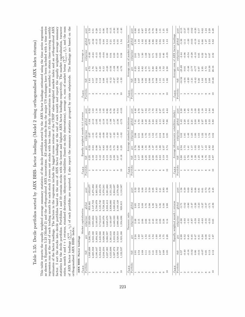
Tab
le5.35
:Decileportfoliossorted
byABX
BBB-factorloadings(M
odel
2usingorthogonalisedABX
index
returns)
This
table
reportsth
eeq
uallyweightedaveragesu
mmary
statisticsofth
edecileportfoliossorted
byth
eABX
factorloadingsestimatedusingth
etimeseries
regression
assh
ownin
Equation5.23(M
odel
2)andth
eorthogonalised
ABX
innovations.
Allavailable
stock
sfrom
themajorUSex
changes
havebeenincluded
withatimeseries
regressionru
natth
een
dofea
chtradingmonth
forea
chstock
(Iscreen
outstock
swithless
than15dailyobservationsin
anymonth
s)to
obtain
time-varyingmonth
lyestimatesofth
efactorloadings.
Thefactors
inth
eregressionincludeth
elagged
excess
retu
rnsofth
eCRSP
value-weightedmarket
index
andanorthogonalised
ABX
factor.
Isort
thestock
sinto
decileportfoliosbased
on
thesu
mofABX
factorloadingsatth
een
dofea
chmonth
and
report
theeq
uallyweighted
averagesu
mmary
statisticsforth
edecileportfolios.
Portfolios1and10co
ntain
stock
swithth
elowestandhighestABX
factorloadingsresp
ectively.
Themarket
capitalisation,tu
rnover
ratios,
month
tandt+
1retu
rns,
standard
dev
iations,
idiosyncraticvolatilities
(basedondailyobservations),averageα,su
mofmarket
betas(∑ 3 j
=1βj),
andth
esu
m
ofABX
factorloadings(∑ 3 j
=1γj)ofea
chportfolioare
reported
.Ialsoreport
thesu
mmary
statisticsgrouped
by
crisis
subperiods.
Thefindingsare
based
on
the
orthogonalisedABX
BBB-index
.
ABX
BBB-Factor
loadin
gs
βA
BX
Mark
etcapitalisa
tion
βA
BX
Equally
weighte
dm
onth
t+1
retu
rns
βA
BX
Avera
geα
Portfolio
full
pre
subprim
eglobal
post
Portfolio
full
pre
subprim
eglobal
post
Portfolio
full
pre
subprim
eglobal
post
11,049,499
1,246,779
1,223,824
953,481
1,053,677
10.25
0.32
-2.07
-1.64
0.52
11.61
4.72
-0.48
-0.77
1.53
22,485,558
2,943,168
2,955,664
2,147,723
2,475,292
20.39
0.63
-1.01
-2.13
1.03
20.57
1.76
-0.24
-0.32
0.51
33,180,447
3,494,163
3,149,857
2,700,978
3,465,564
30.53
0.98
-0.70
-2.05
1.16
30.32
0.97
-0.15
-0.15
0.28
43,354,833
3,449,566
3,712,619
3,125,740
3,432,378
40.43
0.87
-0.80
-1.95
1.00
40.18
0.49
-0.09
-0.03
0.15
53,244,234
3,628,346
3,486,976
2,728,332
3,370,241
50.34
0.83
-0.68
-2.19
1.05
50.08
0.12
-0.04
0.04
0.06
63,227,385
3,088,597
3,645,670
2,933,413
3,381,860
60.19
0.68
-0.92
-2.10
0.86
6-0
.01
-0.20
0.00
0.12
-0.04
73,433,699
3,361,618
4,149,497
2,838,680
3,551,245
70.23
0.79
-0.97
-1.98
0.78
7-0
.12
-0.56
0.04
0.21
-0.15
83,387,272
3,333,936
4,449,333
3,020,953
3,304,697
80.08
0.70
-1.20
-1.97
0.56
8-0
.27
-1.08
0.09
0.33
-0.30
92,526,702
2,520,510
2,888,489
2,160,129
2,578,420
90.07
0.80
-1.49
-2.36
0.54
9-0
.52
-1.96
0.19
0.55
-0.56
10
1,122,537
1,323,188
1,354,696
929,915
1,110,587
10
-0.18
0.29
-1.62
-2.73
-0.03
10
-1.30
-4.76
0.58
1.54
-1.40
βA
BX
Turn
overra
tio
βA
BX
Avera
gestandard
deviations
βA
BX
Avera
gesu
mofm
ark
etrisk
facto
rs
Portfolio
full
pre
subprim
eglobal
post
Portfolio
full
pre
subprim
eglobal
post
Portfolio
full
pre
subprim
eglobal
post
12.81
2.24
2.48
2.65
3.32
15.10
3.78
3.98
7.41
4.48
10.88
0.25
2.61
1.50
0.80
22.54
1.60
2.15
2.54
3.02
23.17
2.26
2.51
4.70
2.78
20.97
0.83
1.67
1.19
0.91
32.68
1.57
2.06
3.09
3.00
32.60
1.86
2.06
3.90
2.27
30.90
0.82
1.30
1.02
0.87
43.11
1.53
2.66
3.76
3.54
42.25
1.55
1.76
3.49
1.94
40.85
0.75
1.08
0.95
0.83
53.21
1.55
2.43
3.98
3.59
52.02
1.38
1.55
3.24
1.72
50.80
0.77
0.87
0.86
0.78
63.41
1.54
2.43
4.36
3.95
62.00
1.37
1.53
3.24
1.70
60.79
0.80
0.71
0.86
0.78
73.03
1.60
2.32
3.67
3.43
72.25
1.55
1.75
3.63
1.94
70.88
0.89
0.65
0.92
0.88
82.87
1.58
2.06
3.36
3.21
82.63
1.88
2.04
4.13
2.27
81.01
1.08
0.63
0.94
1.01
92.68
1.75
2.24
3.30
2.83
93.19
2.37
2.44
4.93
2.75
91.21
1.52
0.46
1.03
1.21
10
3.05
2.28
3.14
2.88
3.38
10
5.18
3.74
3.95
7.88
4.44
10
1.66
2.30
-0.35
1.13
1.65
βA
BX
Equally
weighte
dm
onth
tre
turn
sβA
BX
Avera
geid
iosy
ncra
ticvolatilities(d
aily)
βA
BX
Avera
gesu
mofABX
facto
rloadin
gs
Portfolio
full
pre
subprim
eglobal
post
Portfolio
full
pre
subprim
eglobal
post
Portfolio
full
pre
subprim
eglobal
post
10.57
0.99
-0.90
-5.71
1.56
13.80
2.94
3.02
5.43
3.30
1-1
0.56
-25.89
-2.44
-5.36
-6.15
2-0
.40
0.52
-0.93
-5.02
0.39
22.21
1.73
1.85
3.20
1.86
2-4
.04
-9.81
-0.96
-2.11
-2.27
3-0
.16
0.45
-1.01
-3.80
0.69
31.76
1.41
1.49
2.55
1.45
3-2
.29
-5.46
-0.54
-1.20
-1.23
4-0
.02
0.45
-0.87
-3.47
0.83
41.46
1.17
1.23
2.21
1.18
4-1
.21
-2.77
-0.28
-0.63
-0.62
50.06
0.47
-0.59
-3.26
0.86
51.28
1.03
1.06
2.00
1.00
5-0
.42
-0.77
-0.10
-0.19
-0.20
6-0
.01
0.31
-0.64
-3.23
0.81
61.25
1.02
1.03
1.98
0.99
60.26
0.97
0.05
0.21
0.17
7-0
.07
0.24
-0.63
-3.27
0.61
71.46
1.17
1.22
2.27
1.18
71.03
2.95
0.22
0.66
0.62
80.05
0.08
-0.55
-3.37
0.73
81.76
1.43
1.45
2.69
1.44
82.09
5.72
0.47
1.27
1.24
90.13
0.15
-0.55
-3.71
0.78
92.22
1.82
1.78
3.33
1.84
93.89
10.39
0.87
2.23
2.29
10
2.12
1.67
0.65
-2.36
2.45
10
3.87
2.92
3.02
5.80
3.26
10
10.46
26.16
2.32
5.62
6.28
223

Tab
le5.36
:Decileportfoliossorted
byABX
AAA
factorloadings(M
odel
2usingorthogonalisedABX
index
returnsan
don
lystockswithsign
ificantF-statistics)
This
table
reportsth
eeq
uallyweightedaveragesu
mmary
statisticsofth
edecileportfoliossorted
basedonth
esu
mofABX
factorloadingsestimatedusingth
etimeseries
regressionassh
ownin
Equation5.23(M
odel
2)andth
eorthogonalisedABX
innovations.
Inth
istable,th
edecileportfoliosco
ntain
only
stock
swithsignifica
ntF-statistics
ofnull
hypoth
esis:H
0:γ1=
γ2=
γ3=
0,i.e.
Iscreen
outall
stock
swith
insignifica
ntF-statisticsand
sort
only
those
stock
swith
significa
ntex
posu
reto
theABX
index
.Ith
ensort
thesignifica
ntstock
sinto
decileportfoliosbasedonth
esu
mofABX
factorloadingsatth
een
dofea
chmonth
andreport
theeq
uallyweightedaverage
summary
statistics.
Portfolios1and10co
ntain
stock
swithth
elowestandhighestABX
factorloadingsresp
ectively.
Themarket
capitalisation,tu
rnover
ratios,
month
tandt+
1retu
rns,
standard
dev
iations,
idiosyncraticvolatilities
(basedondailyobservations),averageα,su
mofmarket
betas(∑ 3 j
=1βj),
andth
esu
mofABX
factor
loadings(∑ 3 j
=1γj)ofea
chportfolioare
reported
.Ialsoreport
thesu
mmary
statisticsgrouped
bycrisis
subperiods.
Thefindingsare
basedonth
eABX
AAA
index
.
ABX
AA
AFactor
loadin
gs
βA
BX
Mark
etcapitalisa
tion
βA
BX
Equally
weighte
dm
onth
t+1
retu
rns
βA
BX
Avera
geα
Portfolio
full
pre
subprim
eglobal
post
Portfolio
full
pre
subprim
eglobal
post
Portfolio
full
pre
subprim
eglobal
post
11,138,961
1,143,326
1,779,754
1,040,286
1,045,705
10.60
1.03
-1.46
-1.01
0.36
10.45
-0.07
-0.04
-0.08
1.04
23,150,694
4,261,204
3,730,685
2,549,257
3,089,211
20.65
1.03
-1.08
-2.15
1.46
20.15
-0.08
-0.05
-0.01
0.37
34,121,121
5,423,084
4,928,724
3,237,447
3,877,896
30.40
1.14
-0.99
-2.22
1.18
30.08
-0.06
-0.04
0.02
0.21
43,703,527
3,871,840
4,548,053
2,952,885
3,491,971
40.53
0.97
-0.66
-1.61
1.04
40.05
-0.05
-0.03
0.05
0.11
53,159,799
3,484,707
4,416,844
2,397,010
2,943,333
50.26
0.90
-0.78
-2.35
0.98
50.02
-0.01
-0.05
0.07
0.04
63,387,993
4,033,050
4,584,304
2,510,770
3,316,941
60.23
0.70
-0.83
-2.19
0.85
60.00
0.00
-0.05
0.11
-0.02
73,308,900
4,074,234
4,105,209
2,546,472
3,208,420
70.08
0.75
-0.98
-2.41
0.69
7-0
.03
0.03
-0.04
0.16
-0.12
83,389,836
3,773,882
3,912,584
2,957,875
3,197,059
80.03
1.00
-1.31
-2.22
0.42
8-0
.09
-0.03
-0.05
0.15
-0.23
92,644,394
2,770,210
3,003,046
2,886,958
2,430,835
9-0
.01
0.78
-1.55
-2.46
0.54
9-0
.16
-0.03
-0.08
0.25
-0.42
10
1,152,731
1,676,519
1,158,086
1,172,114
1,071,353
10
-0.23
0.17
-2.41
-2.25
-0.23
10
-0.34
-0.01
0.00
0.51
-0.99
βA
BX
Turn
overra
tio
βA
BX
Avera
gestandard
deviations
βA
BX
Avera
gesu
mofm
ark
etrisk
facto
rs
Portfolio
full
pre
subprim
eglobal
post
Portfolio
full
pre
subprim
eglobal
post
Portfolio
full
pre
subprim
eglobal
post
12.66
2.15
2.33
2.88
2.93
14.62
3.40
3.58
6.98
3.99
1-0
.22
-7.42
-2.00
2.60
1.45
22.71
1.54
2.16
3.17
3.14
22.93
2.09
2.26
4.51
2.51
20.53
-2.67
-0.29
1.78
1.26
32.91
1.89
2.24
3.39
3.29
32.43
1.69
1.88
3.83
2.07
30.62
-1.18
0.09
1.35
1.05
42.98
1.84
2.44
3.03
3.62
42.08
1.50
1.60
3.23
1.77
40.70
-0.30
0.44
1.10
0.93
53.27
1.76
2.80
3.39
3.65
51.90
1.28
1.48
3.07
1.59
50.77
0.42
0.68
1.01
0.78
63.69
1.77
3.24
5.20
3.65
61.94
1.36
1.54
3.07
1.64
60.92
1.08
0.99
1.01
0.78
73.42
1.97
4.93
3.03
3.37
72.16
1.54
1.75
3.37
1.83
71.11
1.96
1.35
0.99
0.80
82.78
2.28
1.93
3.57
2.98
82.48
1.83
1.96
3.77
2.13
81.40
3.32
1.75
1.01
0.78
92.91
1.80
1.94
3.32
3.64
92.97
2.23
2.38
4.36
2.57
91.90
5.46
2.51
1.05
0.89
10
2.82
2.34
2.58
3.19
2.98
10
4.70
3.59
3.68
6.94
4.07
10
3.12
10.95
4.47
0.98
1.05
βA
BX
Equally
weighte
dm
onth
tre
turn
sβA
BX
Avera
geid
iosy
ncra
ticvolatilities(d
aily)
βA
BX
Avera
gesu
mofABX
facto
rloadin
gs
Portfolio
full
pre
subprim
eglobal
post
Portfolio
full
pre
subprim
eglobal
post
Portfolio
full
pre
subprim
eglobal
post
11.53
2.30
1.10
-2.95
0.72
12.98
2.34
2.37
4.38
2.53
1-4
4.01
-159.82
-66.13
-9.84
-14.28
20.22
0.61
-0.33
-3.28
0.21
21.74
1.39
1.46
2.60
1.41
2-1
8.95
-70.78
-27.43
-4.54
-5.67
30.14
0.70
-0.57
-2.65
0.39
31.38
1.10
1.18
2.13
1.09
3-1
1.11
-42.40
-15.69
-2.70
-3.13
40.18
0.56
-0.39
-2.80
0.70
41.15
0.98
0.97
1.75
0.89
4-5
.93
-23.67
-7.73
-1.49
-1.52
50.00
0.54
-0.61
-3.22
0.62
51.02
0.81
0.86
1.63
0.78
5-1
.79
-8.64
-1.24
-0.55
-0.29
60.08
0.24
-0.84
-3.41
1.03
61.04
0.86
0.90
1.60
0.81
61.97
5.25
4.29
0.37
0.85
70.11
0.80
-0.87
-3.73
1.12
71.20
1.00
1.05
1.81
0.94
76.22
20.71
10.77
1.37
2.15
8-0
.22
0.10
-0.91
-4.25
0.90
81.43
1.19
1.22
2.09
1.16
811.72
40.97
18.83
2.69
3.88
9-0
.22
0.05
-1.19
-4.39
0.82
91.80
1.47
1.53
2.54
1.48
920.45
74.09
31.15
4.53
6.53
10
0.68
-0.23
-0.91
-5.00
1.70
10
3.05
2.45
2.47
4.41
2.57
10
46.34
170.35
66.76
10.21
15.41
224

Tab
le5.37:Decileportfoliossorted
byABX
AA
factorloadings(M
odel
2usingorthogonalisedABX
index
returnsandon
lystocks
withsign
ificantF-statistics)
This
table
reportsth
eeq
uallyweightedaveragesu
mmary
statisticsofth
edecileportfoliossorted
basedonth
esu
mofABX
factorloadingsestimatedusingth
etimeseries
regressionassh
ownin
Equation5.23(M
odel
2)andth
eorthogonalisedABX
innovations.
Inth
istable,th
edecileportfoliosco
ntain
only
stock
swithsignifica
ntF-statistics
ofnull
hypoth
esis:H
0:γ1=
γ2=
γ3=
0,i.e.
Iscreen
outall
stock
swith
insignifica
ntF-statisticsand
sort
only
those
stock
swith
significa
ntex
posu
reto
theABX
index
.Ith
ensort
thesignifica
ntstock
sinto
decileportfoliosbasedonth
esu
mofABX
factorloadingsatth
een
dofea
chmonth
andreport
theeq
uallyweightedaverage
summary
statistics.
Portfolios1and10co
ntain
stock
swithth
elowestandhighestABX
factorloadingsresp
ectively.
Themarket
capitalisation,tu
rnover
ratios,
month
tandt+
1retu
rns,
standard
dev
iations,
idiosyncraticvolatilities
(basedondailyobservations),averageα,su
mofmarket
betas(∑ 3 j
=1βj),
andth
esu
mofABX
factor
loadings(∑ 3 j
=1γj)ofea
chportfolioare
reported
.Ialsoreport
thesu
mmary
statisticsgrouped
bycrisis
subperiods.
Thefindingsare
basedonth
eABX
AA
index
.
ABX
AA
Factor
loadin
gs
βA
BX
Mark
etcapitalisa
tion
βA
BX
Equally
weighte
dm
onth
t+1
retu
rns
βA
BX
Avera
geα
Portfolio
full
pre
subprim
eglobal
post
Portfolio
full
pre
subprim
eglobal
post
Portfolio
full
pre
subprim
eglobal
post
11,086,446
908,057
1,344,883
1,074,658
1,129,462
10.41
0.35
-2.60
-1.03
0.52
11.33
5.13
2.02
-0.72
0.93
22,744,808
2,650,041
3,003,292
2,271,670
3,037,346
20.41
1.12
-1.27
-2.11
0.95
20.57
2.34
0.79
-0.33
0.37
33,931,510
3,349,826
3,904,386
3,180,914
4,630,838
30.38
1.39
-1.00
-2.17
0.93
30.36
1.46
0.46
-0.14
0.22
43,627,756
3,055,589
4,627,950
3,185,481
3,611,245
40.26
0.95
-0.86
-2.54
1.05
40.21
0.89
0.25
-0.08
0.13
53,192,304
3,619,860
4,085,146
2,652,119
3,141,021
50.34
0.93
-0.93
-1.94
0.88
50.12
0.44
0.10
0.07
0.05
63,044,842
3,177,180
3,731,253
2,440,979
3,178,048
60.13
0.78
-0.84
-2.24
0.75
60.02
0.00
-0.04
0.12
-0.01
73,656,890
3,720,886
4,729,430
2,627,060
3,753,096
70.13
0.70
-1.30
-2.12
0.88
7-0
.10
-0.52
-0.18
0.24
-0.11
83,470,250
4,539,261
4,271,659
2,723,096
3,294,391
80.22
0.85
-0.89
-2.54
0.94
8-0
.24
-1.14
-0.39
0.37
-0.21
92,901,129
3,356,897
3,489,906
2,602,250
2,831,071
90.47
1.05
-0.86
-1.36
0.60
9-0
.45
-2.10
-0.68
0.60
-0.37
10
1,091,066
1,472,735
1,122,750
1,096,066
1,041,842
10
-0.16
-0.21
-0.66
-2.49
-0.07
10
-1.08
-5.07
-1.67
1.31
-0.82
βA
BX
Turn
overra
tio
βA
BX
Avera
gestandard
deviations
βA
BX
Avera
gesu
mofm
ark
etbeta
s
Portfolio
full
pre
subprim
eglobal
post
Portfolio
full
pre
subprim
eglobal
post
Portfolio
full
pre
subprim
eglobal
post
12.65
1.92
2.41
2.58
3.06
14.60
3.38
3.66
6.83
4.04
1-0
.20
-9.58
-2.09
3.06
1.85
22.85
1.56
2.12
2.86
3.44
22.92
2.13
2.35
4.36
2.56
20.42
-3.92
-0.37
1.97
1.36
32.76
1.38
2.10
3.40
3.14
32.43
1.78
1.93
3.74
2.11
30.54
-2.13
0.14
1.43
1.12
43.10
1.66
2.49
3.88
3.41
42.10
1.51
1.63
3.30
1.79
40.58
-1.10
0.23
1.21
0.95
53.36
1.69
2.70
4.22
3.57
51.96
1.36
1.51
3.17
1.65
50.70
-0.06
0.54
1.05
0.84
63.39
1.71
3.52
3.97
3.48
61.97
1.31
1.51
3.22
1.66
60.86
0.91
0.86
1.02
0.75
72.92
1.64
2.55
3.47
3.15
72.12
1.42
1.64
3.41
1.81
71.02
1.97
1.12
0.90
0.74
82.75
1.68
1.98
3.15
3.19
82.45
1.68
1.93
3.83
2.10
81.29
3.55
1.48
0.71
0.77
92.55
1.92
2.05
2.76
2.84
92.98
2.10
2.27
4.52
2.60
91.65
5.51
2.16
0.59
0.69
10
2.82
2.29
2.21
2.28
3.63
10
4.72
3.40
3.59
7.09
4.12
10
2.86
12.15
4.18
0.28
0.61
βA
BX
Equally
weighte
dm
onth
tre
turn
sβA
BX
Avera
geid
iosy
ncra
ticvolatilities(d
aily)
βA
BX
Avera
gesu
mofABX
facto
rloadin
gs
Portfolio
full
pre
subprim
eglobal
post
Portfolio
full
pre
subprim
eglobal
post
Portfolio
full
pre
subprim
eglobal
post
10.67
1.62
1.48
-4.23
-0.04
12.98
2.31
2.41
4.30
2.58
1-2
1.50
-84.55
-34.12
-3.45
-4.38
2-0
.10
0.02
-0.50
-4.00
0.47
21.74
1.41
1.50
2.52
1.45
2-9
.69
-39.75
-14.30
-1.52
-1.83
30.13
0.28
-0.88
-2.81
0.62
31.40
1.15
1.20
2.12
1.14
3-5
.96
-24.79
-8.73
-0.90
-1.06
4-0
.01
0.29
-0.90
-3.11
0.77
41.17
0.96
0.99
1.79
0.92
4-3
.47
-14.83
-4.94
-0.48
-0.55
50.27
0.61
-0.76
-2.68
1.10
51.06
0.87
0.88
1.68
0.83
5-1
.56
-7.07
-2.13
-0.15
-0.18
60.09
0.40
-0.62
-3.62
1.13
61.07
0.82
0.88
1.70
0.83
60.12
-0.13
0.19
0.17
0.17
7-0
.03
0.08
-0.60
-3.62
1.00
71.17
0.91
0.97
1.81
0.94
72.02
7.91
2.58
0.52
0.57
8-0
.01
0.36
-0.94
-3.70
1.01
81.42
1.10
1.21
2.16
1.14
84.49
18.10
5.94
0.97
1.08
90.21
0.33
-0.65
-3.82
1.14
91.80
1.41
1.45
2.64
1.49
98.36
34.14
11.18
1.62
1.90
10
1.62
1.40
-0.82
-3.98
2.64
10
3.09
2.37
2.42
4.56
2.60
10
20.39
83.69
27.56
3.65
4.57
225

Tab
le5.38
:Decileportfoliossorted
byABX
Afactorloadings(M
odel
2usingorthogonalisedABX
index
returnsandon
lystocks
withsign
ificantF-statistics)
This
table
reportsth
eeq
uallyweightedaveragesu
mmary
statisticsofth
edecileportfoliossorted
basedonth
esu
mofABX
factorloadingsestimatedusingth
etimeseries
regressionassh
ownin
Equation5.23(M
odel
2)andth
eorthogonalisedABX
innovations.
Inth
istable,th
edecileportfoliosco
ntain
only
stock
swithsignifica
ntF-statistics
ofnull
hypoth
esis:H
0:γ1=
γ2=
γ3=
0,i.e.
Iscreen
outall
stock
swith
insignifica
ntF-statisticsand
sort
only
those
stock
swith
significa
ntex
posu
reto
theABX
index
.Ith
ensort
thesignifica
ntstock
sinto
decileportfoliosbasedonth
esu
mofABX
factorloadingsatth
een
dofea
chmonth
andreport
theeq
uallyweightedaverage
summary
statistics.
Portfolios1and10co
ntain
stock
swithth
elowestandhighestABX
factorloadingsresp
ectively.
Themarket
capitalisation,tu
rnover
ratios,
month
tandt+
1retu
rns,
standard
dev
iations,
idiosyncraticvolatilities
(basedondailyobservations),averageα,su
mofmarket
betas(∑ 3 j
=1βj),
andth
esu
mofABX
factor
loadings(∑ 3 j
=1γj)ofea
chportfolioare
reported
.Ialsoreport
thesu
mmary
statisticsgrouped
bycrisis
subperiods.
Thefindingsare
basedonth
eABX
Aindex
.
ABX
AFactor
loadin
gs
βA
BX
Mark
etcapitalisa
tion
βA
BX
Equally
weighte
dm
onth
t+1
retu
rns
βA
BX
Avera
geα
Portfolio
full
pre
subprim
eglobal
post
Portfolio
full
pre
subprim
eglobal
post
Portfolio
full
pre
subprim
eglobal
post
1975,662
1,186,407
1,511,720
918,012
805,528
10.16
-0.10
-1.54
-1.89
0.25
12.48
13.27
0.96
-1.22
1.02
22,690,038
3,020,214
3,405,886
2,704,207
2,386,082
20.40
0.47
-1.20
-1.43
0.86
21.10
6.09
0.41
-0.58
0.43
33,628,703
3,342,545
4,583,746
3,096,275
3,703,086
30.57
0.72
-0.99
-1.78
1.36
30.67
3.74
0.24
-0.32
0.25
43,612,424
3,795,374
4,544,186
2,839,364
3,618,992
40.52
0.90
-0.38
-2.06
1.33
40.40
2.10
0.15
-0.11
0.15
53,319,650
3,514,597
3,684,189
3,369,201
3,330,096
50.48
0.94
-0.48
-1.64
1.03
50.20
0.91
0.09
0.03
0.06
63,355,022
3,449,380
3,606,813
2,719,800
3,711,367
60.36
0.70
-0.64
-1.56
0.91
60.00
-0.09
0.00
0.13
-0.02
73,617,897
3,878,797
4,957,999
2,785,187
3,557,936
70.38
0.96
-0.86
-1.89
1.10
7-0
.19
-1.25
-0.07
0.26
-0.10
83,473,400
3,086,848
4,002,400
2,234,127
4,105,101
80.09
1.07
-1.18
-2.27
0.73
8-0
.47
-2.81
-0.18
0.46
-0.22
92,708,458
2,932,775
3,317,340
1,846,468
2,937,091
90.06
0.77
-1.35
-2.91
0.92
9-0
.93
-5.40
-0.30
0.71
-0.42
10
1,307,959
1,453,379
1,239,125
1,608,396
1,202,265
10
-0.13
0.00
-1.54
-2.20
-0.20
10
-2.22
-13.11
-0.68
1.81
-1.01
βA
BX
Turn
overra
tio
βA
BX
Avera
gestandard
deviations
βA
BX
Avera
gesu
mofm
ark
etbeta
s
Portfolio
full
pre
subprim
eglobal
post
Portfolio
full
pre
subprim
eglobal
post
Portfolio
full
pre
subprim
eglobal
post
12.94
2.05
2.21
4.81
2.84
14.69
3.36
3.73
6.79
4.17
10.08
-7.44
2.09
3.11
0.82
22.59
1.60
1.95
3.31
2.79
22.98
2.10
2.28
4.46
2.66
20.54
-2.97
1.43
1.95
0.88
32.76
1.64
2.08
3.55
2.86
32.45
1.75
1.90
3.62
2.21
30.64
-1.63
1.19
1.39
0.95
43.01
1.62
2.50
4.24
3.07
42.14
1.44
1.65
3.30
1.89
40.65
-0.51
0.91
1.07
0.76
53.26
1.61
3.21
4.32
3.34
51.95
1.29
1.47
3.13
1.69
50.70
0.19
0.71
0.96
0.74
63.35
1.64
3.54
3.28
3.91
61.97
1.34
1.51
3.30
1.64
60.78
0.81
0.70
0.81
0.75
73.33
1.53
2.47
4.21
3.63
72.13
1.45
1.69
3.46
1.77
70.90
1.69
0.58
0.63
0.82
82.90
1.59
2.23
3.94
2.87
82.49
1.75
1.99
4.01
2.08
81.10
2.68
0.48
0.52
0.94
92.67
2.01
2.05
2.99
2.79
92.96
2.20
2.31
4.56
2.53
91.40
4.55
0.24
0.32
1.04
10
2.81
2.17
2.54
2.73
3.25
10
4.72
3.49
3.70
7.17
4.11
10
2.40
10.19
-0.19
-0.32
1.51
βA
BX
Equally
weighte
dm
onth
tre
turn
sβA
BX
Avera
geid
iosy
ncra
ticvolatilities(d
aily)
βA
BX
Avera
gesu
mofABX
facto
rloadin
gs
Portfolio
full
pre
subprim
eglobal
post
Portfolio
full
pre
subprim
eglobal
post
Portfolio
full
pre
subprim
eglobal
post
11.40
1.80
1.39
-3.05
1.14
13.05
2.32
2.47
4.27
2.67
1-2
2.14
-105.65
-10.47
-3.24
-5.83
2-0
.22
0.78
-0.41
-4.08
0.24
21.80
1.39
1.47
2.61
1.54
2-9
.99
-48.55
-4.57
-1.34
-2.52
3-0
.13
0.71
-0.91
-3.06
0.35
31.42
1.15
1.18
2.02
1.21
3-6
.06
-29.65
-2.87
-0.75
-1.49
40.06
0.64
-0.51
-2.73
0.34
41.20
0.94
0.99
1.79
1.00
4-3
.45
-16.95
-1.74
-0.35
-0.83
50.18
0.43
-0.25
-2.65
0.66
51.06
0.83
0.87
1.64
0.86
5-1
.47
-7.43
-0.79
-0.04
-0.33
6-0
.11
0.20
-0.94
-3.38
0.82
61.06
0.85
0.88
1.73
0.82
60.22
0.56
0.03
0.29
0.12
70.02
0.12
-0.92
-3.77
1.09
71.19
0.94
1.02
1.87
0.93
72.10
9.61
0.83
0.65
0.59
80.03
0.51
-0.82
-3.74
1.04
81.45
1.16
1.23
2.27
1.15
84.72
22.39
1.84
1.09
1.23
9-0
.08
-0.01
-0.93
-4.10
0.95
91.79
1.47
1.48
2.67
1.47
98.81
42.52
3.42
1.76
2.22
10
0.98
0.63
-1.31
-4.67
2.22
10
3.09
2.41
2.48
4.56
2.64
10
21.58
103.95
8.49
3.99
5.74
226

Tab
le5.39
:Decileportfoliossorted
byABX
BBB
factorloadings(M
odel
2usingorthogonalisedABX
index
returnsan
don
lystockswithsign
ificantF-statistics)
This
table
reportsth
eeq
uallyweightedaveragesu
mmary
statisticsofth
edecileportfoliossorted
basedonth
esu
mofABX
factorloadingsestimatedusingth
etimeseries
regressionassh
ownin
Equation5.23(M
odel
2)andth
eorthogonalisedABX
innovations.
Inth
istable,th
edecileportfoliosco
ntain
only
stock
swithsignifica
ntF-statistics
ofnull
hypoth
esis:H
0:γ1=
γ2=
γ3=
0,i.e.
Iscreen
outall
stock
swith
insignifica
ntF-statisticsand
sort
only
those
stock
swith
significa
ntex
posu
reto
theABX
index
.Ith
ensort
thesignifica
ntstock
sinto
decileportfoliosbasedonth
esu
mofABX
factorloadingsatth
een
dofea
chmonth
andreport
theeq
uallyweightedaverage
summary
statistics.
Portfolios1and10co
ntain
stock
swithth
elowestandhighestABX
factorloadingsresp
ectively.
Themarket
capitalisation,tu
rnover
ratios,
month
tandt+
1retu
rns,
standard
dev
iations,
idiosyncraticvolatilities
(basedondailyobservations),averageα,su
mofmarket
betas(∑ 3 j
=1βj),
andth
esu
mofABX
factor
loadings(∑ 3 j
=1γj)ofea
chportfolioare
reported
.Ialsoreport
thesu
mmary
statisticsgrouped
bycrisis
subperiods.
Thefindingsare
basedonth
eABX
BBB
index
.
ABX
BBB
Factor
loadin
gs
βA
BX
Mark
etcapitalisa
tion
βA
BX
Equally
weighte
dm
onth
t+1
retu
rns
βA
BX
Avera
geα
Portfolio
full
pre
subprim
eglobal
post
Portfolio
full
pre
subprim
eglobal
post
Portfolio
full
pre
subprim
eglobal
post
11,085,559
1,291,876
1,312,656
1,007,191
1,057,582
10.03
0.71
-1.90
-2.37
-0.24
12.41
7.82
-0.07
-0.65
2.02
22,721,617
3,617,960
2,753,696
2,299,426
2,816,008
20.45
0.94
-0.84
-2.11
0.88
21.00
3.41
-0.06
-0.20
0.80
33,755,900
4,365,756
4,242,782
3,146,594
3,946,355
30.24
0.56
-0.57
-1.85
0.54
30.58
2.01
-0.04
-0.06
0.44
43,602,325
3,886,650
3,859,572
3,286,726
3,744,514
40.29
0.71
-0.82
-1.95
0.71
40.34
1.09
-0.02
0.05
0.24
53,330,102
3,334,280
3,517,488
3,119,689
3,281,998
50.35
1.00
-0.61
-2.33
0.98
50.14
0.31
0.01
0.14
0.06
63,243,568
3,456,032
3,338,914
3,162,393
3,218,165
60.10
0.94
-0.94
-2.28
0.73
6-0
.05
-0.37
0.02
0.19
-0.10
73,684,704
4,524,173
5,080,753
3,001,789
3,312,843
70.24
1.30
-0.84
-2.30
0.66
7-0
.23
-1.16
0.04
0.31
-0.27
83,413,749
3,806,503
4,413,161
2,937,384
3,238,842
80.12
1.11
-1.20
-2.70
0.70
8-0
.52
-2.13
0.04
0.39
-0.56
92,778,993
2,642,902
3,468,661
2,759,231
2,585,465
90.34
0.81
-0.91
-2.22
1.10
9-0
.97
-3.78
0.06
0.55
-0.97
10
1,149,944
1,279,922
1,312,187
1,346,172
939,383
10
-0.41
0.53
-2.12
-2.44
-0.45
10
-2.25
-8.60
0.12
1.42
-2.25
βA
BX
Turn
overra
tio
βA
BX
Avera
gestandard
deviations
βA
BX
Avera
gesu
mofm
ark
etbeta
s
Portfolio
full
pre
subprim
eglobal
post
Portfolio
full
pre
subprim
eglobal
post
Portfolio
full
pre
subprim
eglobal
post
12.85
2.18
2.39
3.25
3.11
14.66
3.37
3.78
6.78
3.99
10.96
2.35
2.95
1.43
0.64
22.56
1.85
2.10
3.03
2.67
22.92
2.11
2.36
4.37
2.48
20.93
1.65
1.74
1.22
0.66
32.69
2.16
2.12
3.48
2.65
32.42
1.69
1.95
3.69
2.04
30.93
1.31
1.34
1.12
0.77
42.82
1.51
2.81
3.57
2.89
42.13
1.50
1.72
3.34
1.79
40.86
1.13
1.10
0.98
0.73
53.34
1.59
2.35
3.98
3.80
51.97
1.33
1.52
3.25
1.62
50.84
1.01
0.85
0.93
0.77
63.25
1.64
2.57
4.21
3.15
61.97
1.33
1.50
3.24
1.66
60.82
0.80
0.67
0.81
0.86
73.63
1.51
2.19
4.09
4.43
72.13
1.45
1.64
3.37
1.88
70.85
0.73
0.61
0.79
0.93
83.03
1.60
3.28
4.10
2.85
82.48
1.76
1.91
3.83
2.21
80.96
0.70
0.47
0.79
1.14
92.99
1.84
1.93
3.68
3.47
93.00
2.18
2.25
4.51
2.71
91.20
0.77
0.28
1.02
1.46
10
3.29
2.31
2.35
5.65
2.85
10
4.70
3.48
3.53
7.04
4.20
10
1.64
0.55
-0.53
1.37
2.09
βA
BX
Equally
weighte
dm
onth
tre
turn
sβA
BX
Avera
geid
iosy
ncra
ticvolatilities(d
aily)
βA
BX
Avera
gesu
mofABX
facto
rloadin
gs
Portfolio
full
pre
subprim
eglobal
post
Portfolio
full
pre
subprim
eglobal
post
Portfolio
full
pre
subprim
eglobal
post
11.30
2.08
0.63
-4.73
1.48
13.04
2.33
2.52
4.28
2.55
1-1
5.07
-45.13
-4.34
-6.21
-7.97
20.13
0.81
-0.81
-3.81
0.80
21.77
1.40
1.53
2.55
1.42
2-6
.35
-19.88
-1.89
-2.72
-3.17
3-0
.17
0.55
-0.93
-3.61
0.26
31.40
1.09
1.21
2.06
1.10
3-3
.72
-11.78
-1.16
-1.68
-1.80
40.12
0.77
-0.67
-2.84
0.68
41.19
0.98
1.05
1.78
0.93
4-2
.04
-6.45
-0.68
-0.98
-0.93
50.17
0.58
-0.74
-2.92
0.81
51.06
0.85
0.91
1.66
0.81
5-0
.74
-2.10
-0.30
-0.41
-0.25
60.10
0.28
-0.81
-2.73
0.87
61.05
0.86
0.87
1.67
0.81
60.44
1.83
0.01
0.14
0.37
70.12
0.30
-0.71
-3.15
1.03
71.18
0.96
0.97
1.79
0.96
71.75
6.28
0.33
0.73
1.09
8-0
.04
0.75
-0.63
-3.65
0.69
81.42
1.16
1.15
2.09
1.20
83.47
11.92
0.77
1.47
2.09
9-0
.31
0.18
-0.83
-4.52
0.70
91.80
1.46
1.44
2.61
1.56
96.23
21.12
1.44
2.60
3.67
10
0.61
1.32
-0.74
-4.94
1.51
10
3.05
2.39
2.37
4.42
2.67
10
14.99
49.01
3.55
6.18
8.86
227

Tab
le5.40
:Decileportfoliossorted
byABX
BBB-factorloadings(M
odel
2usingorthogonalisedABX
index
returnsan
don
lystockswithsign
ificantF-statistics)
This
table
reportsth
eeq
uallyweighted
averagesu
mmary
statisticsofth
edecileportfoliossorted
based
on
thesu
mofABX
factorloadingsestimated
usingth
etime
series
regressionassh
ownin
Equation5.23(M
odel
2)andth
eorthogonalised
ABX
innovations.
Inth
istable,th
edecileportfoliosco
ntain
only
stock
swithsignifica
nt
F-statisticsofnullhypoth
esis:H
0:γ1=
γ2=
γ3=
0,i.e.
Iscreen
outallstock
swithinsignifica
ntF-statisticsandsort
only
those
stock
swithsignifica
ntex
posu
reto
the
ABX
index
.Ith
ensort
thesignifica
ntstock
sinto
decileportfoliosbasedonth
esu
mofABX
factorloadingsatth
een
dofea
chmonth
andreport
theeq
uallyweighted
averagesu
mmary
statistics.
Portfolios1and10co
ntain
stock
swithth
elowestandhighestABX
factorloadingsresp
ectively.
Themarket
capitalisation,tu
rnover
ratios,
month
tandt+
1retu
rns,
standard
dev
iations,
idiosyncraticvolatilities
(basedondailyobservations),averageα,su
mofmarket
betas(∑ 3 j
=1βj),
andth
esu
mofABX
factorloadings(∑ 3 j
=1γj)ofea
chportfolioare
reported
.Ialsoreport
thesu
mmary
statisticsgrouped
bycrisis
subperiods.
Thefindingsare
basedonth
eABX
BBB-
index
.
ABX
BBB-Factor
loadin
gs
βA
BX
Mark
etcapitalisa
tion
βA
BX
Equally
weighte
dm
onth
t+1
retu
rns
βA
BX
Avera
geα
Portfolio
full
pre
subprim
eglobal
post
Portfolio
full
pre
subprim
eglobal
post
Portfolio
full
pre
subprim
eglobal
post
11,074,772
1,269,320
1,537,446
919,407
1,006,320
10.38
0.04
-2.52
-1.46
0.70
11.85
5.76
-0.44
-0.93
1.79
22,689,478
3,436,525
3,205,823
2,265,652
2,609,302
20.39
0.73
-0.73
-2.27
0.88
20.76
2.45
-0.25
-0.38
0.70
33,666,655
4,490,843
3,896,903
2,859,610
3,838,992
30.41
1.03
-0.55
-2.70
1.24
30.46
1.44
-0.16
-0.16
0.39
43,654,014
3,371,773
4,067,088
3,350,495
3,899,579
40.42
1.52
-0.97
-2.25
1.05
40.27
0.80
-0.09
-0.03
0.21
53,302,861
3,279,989
3,939,082
2,768,752
3,396,596
50.21
0.69
-0.63
-2.30
0.80
50.13
0.24
-0.02
0.07
0.07
63,256,553
3,500,141
3,503,975
3,232,130
3,210,967
60.15
0.69
-0.81
-2.00
0.58
6-0
.01
-0.24
0.04
0.15
-0.07
73,730,091
3,171,809
5,295,243
3,375,607
3,646,618
70.14
0.97
-0.88
-2.15
0.51
7-0
.18
-0.78
0.07
0.28
-0.26
83,660,871
3,632,912
5,233,816
2,977,999
3,441,413
8-0
.13
0.91
-1.42
-2.73
0.38
8-0
.38
-1.49
0.15
0.42
-0.46
92,797,735
2,892,872
3,297,634
2,382,242
2,766,890
9-0
.06
1.17
-1.71
-2.53
0.32
9-0
.70
-2.57
0.22
0.64
-0.79
10
1,104,961
1,216,222
1,393,588
1,014,164
1,004,206
10
-0.03
0.57
-1.21
-2.78
0.05
10
-1.68
-5.83
0.54
1.55
-1.84
βA
BX
Turn
overra
tio
βA
BX
Avera
gestandard
deviations
βA
BX
Avera
gesu
mofm
ark
etbeta
s
Portfolio
full
pre
subprim
eglobal
post
Portfolio
full
pre
subprim
eglobal
post
Portfolio
full
pre
subprim
eglobal
post
12.61
2.13
2.53
2.56
2.85
14.66
3.44
3.77
6.67
4.14
10.81
-0.02
2.86
1.39
0.76
22.84
1.59
2.23
3.56
3.01
22.94
2.07
2.30
4.43
2.55
20.88
0.59
1.80
1.12
0.82
32.75
1.96
2.47
3.22
2.83
32.43
1.74
1.97
3.68
2.09
30.86
0.72
1.41
0.98
0.85
43.16
1.79
3.20
3.44
3.42
42.14
1.48
1.69
3.33
1.81
40.80
0.63
1.18
0.86
0.80
53.22
1.51
2.46
3.91
3.62
51.96
1.36
1.55
3.16
1.64
50.79
0.75
0.90
0.80
0.81
63.38
1.76
2.83
4.16
3.77
61.96
1.36
1.52
3.22
1.65
60.78
0.78
0.70
0.81
0.78
73.29
1.63
2.29
3.89
3.98
72.16
1.48
1.69
3.47
1.87
70.86
0.91
0.61
0.82
0.88
83.00
1.63
2.88
3.65
2.99
82.47
1.72
1.88
3.91
2.18
81.01
1.19
0.48
0.81
1.10
93.06
1.74
1.95
4.26
3.19
92.97
2.13
2.27
4.48
2.64
91.22
1.69
0.27
0.90
1.27
10
3.28
2.27
2.54
3.59
3.88
10
4.70
3.41
3.52
7.20
4.07
10
1.80
2.91
-0.51
1.05
1.82
βA
BX
Equally
weighte
dm
onth
tre
turn
sβA
BX
Avera
geid
iosy
ncra
ticvolatilities(d
aily)
βA
BX
Avera
gesu
mofABX
facto
rloadin
gs
Portfolio
full
pre
subprim
eglobal
post
Portfolio
full
pre
subprim
eglobal
post
Portfolio
full
pre
subprim
eglobal
post
10.27
0.39
1.76
-6.25
0.65
13.06
2.39
2.52
4.25
2.65
1-1
2.31
-31.62
-3.11
-6.36
-7.42
2-0
.54
0.63
-0.90
-4.58
-0.07
21.78
1.39
1.48
2.60
1.46
2-5
.30
-13.61
-1.34
-2.78
-2.98
3-0
.20
0.68
-0.85
-3.73
0.53
31.41
1.13
1.23
2.05
1.14
3-3
.14
-8.01
-0.81
-1.64
-1.69
40.08
0.72
-0.75
-2.84
0.66
41.19
0.95
1.03
1.79
0.92
4-1
.76
-4.37
-0.46
-0.91
-0.88
5-0
.01
0.18
-0.75
-3.14
0.90
51.06
0.87
0.92
1.67
0.81
5-0
.68
-1.54
-0.19
-0.30
-0.26
6-0
.01
0.39
-0.46
-3.35
0.90
61.06
0.86
0.90
1.66
0.83
60.31
1.14
0.05
0.25
0.31
7-0
.09
0.53
-0.91
-2.76
0.53
71.19
0.96
1.02
1.84
0.96
71.41
4.17
0.31
0.84
0.99
80.01
0.17
-0.56
-3.23
0.77
81.42
1.13
1.15
2.16
1.17
82.82
7.90
0.64
1.62
1.86
90.06
0.50
-0.70
-3.63
0.81
91.79
1.43
1.44
2.59
1.52
95.05
13.78
1.14
2.75
3.22
10
1.63
2.78
-0.12
-2.90
1.99
10
3.06
2.36
2.36
4.53
2.60
10
12.35
31.97
2.71
6.50
7.83
228

Tab
le5.41
:Decileportfoliossorted
byABX
AAA
factorloadings(M
odel
3usingorthogonalisedABX
index
returns)
This
table
reportsth
eeq
uallyweightedaveragesu
mmary
statisticsofth
edecileportfoliossorted
byth
eABX
factorloadingsestimatedusingth
etimeseries
regression
assh
ownin
Equation5.24(M
odel
3).
Allavailable
stock
sfrom
themajorUSex
changes
havebeenincluded
withatimeseries
regressionru
natth
een
dofea
chtrading
month
forea
chstock
(Iscreen
outstock
swith
less
than
15dailyobservationsin
anymonth
s)to
obtain
time-varyingmonth
lyestimatesofth
efactorloadings.
The
factors
inth
eregressionincludeth
eex
cess
retu
rnsofth
eCRSP
value-weightedmarket
index
,th
eFamaandFrench
(1993)SMB
andHML
factors,th
eCahart
(1997)
Momen
tum
factorandanorthogonalised
ABX
factor.
Isort
thestock
sinto
decileportfoliosbasedonth
eABX
factorloadingsatth
een
dofea
chmonth
andreport
the
equallyweightedaveragesu
mmary
statisticsofth
edecileportfolios.
Portfolios1and10co
ntain
stock
swithth
elowestandhighestABX
factorloadingsresp
ectively.
Themarket
capitalisation,tu
rnover
ratios,
month
tandt+
1retu
rns,
standard
dev
iations,
idiosyncraticvolatilities
(basedondailyobservations),th
eaverageα,βM
KT,
andth
eβABX
ofea
chportfolioare
reported
.Ialsoreport
thesu
mmary
statisticsbasedonmycrisis
subperiods.
Thefindingsare
basedonth
eABX
AAA
index
.
ABX
AA
AFactor
loadin
gs
βA
BX
Mark
etcapitalisa
tion
βA
BX
Equally
weighte
dm
onth
t+1
retu
rns
βA
BX
Avera
geα
Portfolio
full
pre
subprim
eglobal
post
Portfolio
full
pre
subprim
eglobal
post
Portfolio
full
pre
subprim
eglobal
post
1865,759
1,068,618
1,207,737
654,067
806,698
10.11
0.03
-1.18
-2.59
0.48
10.09
0.05
-0.10
-0.21
0.22
22,335,461
2,349,027
2,863,431
1,966,390
2,447,237
20.23
0.85
-1.28
-2.41
0.84
2-0
.01
0.00
-0.07
-0.15
0.05
33,233,799
3,216,956
3,844,539
2,740,320
3,379,786
30.27
0.74
-1.09
-2.26
0.98
30.00
0.00
-0.04
-0.08
0.03
43,485,327
3,654,290
3,831,691
2,856,714
3,701,114
40.33
1.06
-0.80
-2.06
0.88
40.00
0.00
-0.03
-0.06
0.02
53,495,367
3,652,401
3,706,307
3,201,056
3,624,631
50.23
0.78
-0.88
-2.06
0.82
50.00
0.00
-0.01
-0.03
0.01
63,362,414
3,646,045
4,117,652
2,911,042
3,254,497
60.10
0.70
-0.92
-2.27
0.66
60.00
-0.01
-0.02
0.00
0.00
73,704,114
4,103,631
4,363,223
3,176,989
3,701,266
70.30
0.87
-0.90
-1.79
0.85
7-0
.01
0.00
0.00
-0.01
-0.01
83,134,163
3,250,113
3,401,361
3,015,704
3,192,718
80.26
0.75
-1.08
-2.21
0.93
80.00
0.00
0.01
0.03
-0.03
92,276,762
2,319,262
2,599,303
2,127,413
2,265,165
90.41
0.82
-1.27
-1.66
0.87
90.00
0.00
0.03
0.09
-0.06
10
934,351
1,086,762
1,076,543
893,094
908,718
10
0.04
0.25
-2.08
-1.81
0.04
10
0.08
0.08
0.13
0.34
-0.08
βA
BX
Turn
overra
tio
βA
BX
Avera
gestandard
deviations
βA
BX
Avera
geβM
KT
Portfolio
full
pre
subprim
eglobal
post
Portfolio
full
pre
subprim
eglobal
post
Portfolio
full
pre
subprim
eglobal
post
12.57
2.12
2.41
2.16
3.03
15.11
3.74
3.91
7.45
4.51
1-1
.74
-12.52
-0.85
0.68
0.38
22.57
1.78
1.97
2.59
3.04
23.18
2.34
2.43
4.80
2.76
2-0
.13
-4.31
0.23
0.76
0.70
32.64
1.55
2.04
2.99
3.03
32.61
1.90
2.03
4.00
2.22
30.28
-2.05
0.47
0.74
0.75
43.20
1.67
2.50
3.86
3.67
42.26
1.62
1.77
3.54
1.91
40.47
-0.73
0.58
0.72
0.73
53.61
1.68
2.91
4.37
4.02
52.01
1.40
1.56
3.25
1.70
50.60
0.21
0.64
0.65
0.70
63.67
1.72
2.47
4.60
4.22
61.99
1.36
1.58
3.11
1.73
60.76
1.04
0.74
0.69
0.72
73.12
1.51
2.71
4.08
3.31
72.25
1.56
1.76
3.56
1.94
70.99
2.01
0.91
0.75
0.79
82.75
1.49
2.10
3.56
3.04
82.62
1.85
2.06
4.10
2.26
81.28
3.36
1.15
0.79
0.87
92.68
1.65
2.54
2.99
2.86
93.18
2.25
2.48
4.89
2.76
91.72
5.61
1.45
0.85
0.95
10
2.74
2.10
2.33
2.38
3.41
10
5.16
3.74
3.99
7.85
4.44
10
3.10
13.47
2.46
0.77
1.06
βA
BX
Equally
weighte
dm
onth
tre
turn
sβA
BX
Avera
geid
iosy
ncra
ticvolatilities(d
aily)
βA
BX
Avera
geβA
BX
Portfolio
full
pre
subprim
eglobal
post
Portfolio
full
pre
subprim
eglobal
post
Portfolio
full
pre
subprim
eglobal
post
11.07
0.75
0.51
-4.81
1.63
13.95
2.99
3.08
5.64
3.47
1-3
0.93
-161.98
-21.73
-3.05
-3.49
20.01
0.37
-0.59
-4.28
0.78
22.28
1.84
1.81
3.35
1.93
2-1
1.79
-62.02
-8.20
-1.22
-1.24
30.15
0.53
-0.44
-3.61
0.95
31.80
1.48
1.49
2.70
1.46
3-6
.52
-34.30
-4.50
-0.72
-0.67
40.13
0.65
-0.57
-3.50
0.96
41.50
1.25
1.26
2.30
1.19
4-3
.36
-17.83
-2.21
-0.41
-0.33
50.09
0.46
-0.43
-3.19
0.91
51.28
1.05
1.09
2.02
1.00
5-1
.07
-5.78
-0.57
-0.17
-0.09
60.03
0.38
-0.66
-3.04
0.81
61.25
1.03
1.11
1.86
1.03
60.92
4.69
0.81
0.03
0.11
7-0
.07
0.38
-0.73
-3.61
0.80
71.48
1.20
1.27
2.24
1.21
73.13
16.28
2.41
0.25
0.35
8-0
.11
0.30
-0.90
-3.60
0.61
81.79
1.43
1.52
2.68
1.49
86.27
32.69
4.64
0.56
0.70
9-0
.16
0.32
-1.09
-3.94
0.51
92.27
1.76
1.89
3.35
1.93
911.54
60.32
8.36
1.07
1.28
10
1.10
1.18
-1.10
-3.61
1.64
10
3.99
3.00
3.16
5.89
3.41
10
30.41
159.02
21.65
2.86
3.51
229
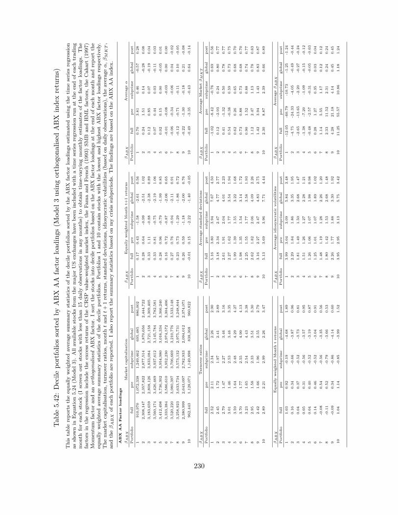
Tab
le5.42
:Decileportfoliossorted
byABX
AA
factorloadings(M
odel
3usingorthogonalisedABX
index
returns)
This
table
reportsth
eeq
uallyweightedaveragesu
mmary
statisticsofth
edecileportfoliossorted
byth
eABX
factorloadingsestimatedusingth
etimeseries
regression
assh
ownin
Equation5.24(M
odel
3).
Allavailable
stock
sfrom
themajorUSex
changes
havebeenincluded
withatimeseries
regressionru
natth
een
dofea
chtrading
month
forea
chstock
(Iscreen
outstock
swith
less
than
15dailyobservationsin
anymonth
s)to
obtain
time-varyingmonth
lyestimatesofth
efactorloadings.
The
factors
inth
eregressionincludeth
eex
cess
retu
rnsofth
eCRSP
value-weightedmarket
index
,th
eFamaandFrench
(1993)SMB
andHML
factors,th
eCahart
(1997)
Momen
tum
factorandanorthogonalised
ABX
factor.
Isort
thestock
sinto
decileportfoliosbasedonth
eABX
factorloadingsatth
een
dofea
chmonth
andreport
the
equallyweightedaveragesu
mmary
statisticsofth
edecileportfolios.
Portfolios1and10co
ntain
stock
swithth
elowestandhighestABX
factorloadingsresp
ectively.
Themarket
capitalisation,tu
rnover
ratios,
month
tandt+
1retu
rns,
standard
dev
iations,
idiosyncraticvolatilities
(basedondailyobservations),th
eaverageα,βM
KT,
andth
eβABX
ofea
chportfolioare
reported
.Ialsoreport
thesu
mmary
statisticsbasedonmycrisis
subperiods.
Thefindingsare
basedonth
eABX
AA
index
.
ABX
AA
Factor
loadin
gs
βA
BX
Mark
etcapitalisa
tion
βA
BX
Equally
weighte
dM
onth
t+1
retu
rns
βA
BX
Avera
geα
Portfolio
full
pre
subprim
eglobal
post
Portfolio
full
pre
subprim
eglobal
post
Portfolio
full
pre
subprim
eglobal
post
1910,970
1,072,338
1,249,462
695,485
886,002
10.17
0.43
-1.58
-2.61
0.56
10.70
3.81
0.46
-0.57
0.28
22,308,147
2,357,822
2,877,514
1,870,656
2,444,722
20.28
0.64
-0.99
-2.51
1.02
20.24
1.51
0.14
-0.28
0.08
33,183,659
2,808,126
3,833,084
2,721,158
3,369,405
30.33
1.11
-0.88
-2.38
0.89
30.12
0.85
0.07
-0.19
0.04
43,560,174
3,426,469
3,937,612
3,145,784
3,782,581
40.33
0.81
-0.75
-2.19
1.06
40.07
0.44
0.03
-0.11
0.03
53,412,498
3,736,302
3,954,980
3,016,334
3,366,240
50.28
0.96
-0.79
-1.99
0.85
50.02
0.15
0.00
-0.05
0.01
63,333,384
3,586,610
3,952,230
2,974,572
3,304,406
60.16
0.72
-0.87
-2.06
0.65
6-0
.01
-0.08
-0.03
0.00
0.00
73,520,220
3,980,397
3,706,669
3,210,776
3,533,148
70.27
0.76
-0.94
-2.11
0.91
7-0
.06
-0.34
-0.06
0.04
-0.02
83,258,923
3,633,734
3,573,132
2,975,731
3,248,844
80.23
0.73
-1.29
-1.86
0.72
8-0
.12
-0.71
-0.11
0.10
-0.05
92,380,999
2,643,097
2,782,933
2,094,012
2,374,071
90.26
0.59
-1.18
-2.00
0.76
9-0
.22
-1.30
-0.18
0.21
-0.08
10
962,443
1,128,071
1,149,898
838,368
960,822
10
-0.01
0.15
-2.22
-1.40
-0.05
10
-0.49
-3.35
-0.43
0.64
-0.14
βA
BX
Turn
overra
tios
βA
BX
Avera
gestandard
deviations
βA
BX
Avera
geM
ark
etβM
KT
Portfolio
full
pre
subprim
eglobal
post
Portfolio
full
pre
subprim
eglobal
post
Portfolio
full
pre
subprim
eglobal
post
12.52
2.11
2.34
2.26
2.90
15.16
3.80
3.94
7.67
4.50
1-1
.02
-8.42
-0.76
0.69
0.56
22.45
1.72
1.97
2.41
2.89
23.18
2.34
2.47
4.77
2.77
20.12
-2.93
0.24
0.80
0.77
32.79
1.47
2.27
3.46
3.16
32.61
1.91
2.04
4.01
2.23
30.41
-1.32
0.50
0.78
0.77
43.01
1.46
2.53
3.46
3.35
42.27
1.62
1.77
3.54
1.94
40.54
-0.38
0.59
0.73
0.75
53.59
1.64
2.48
4.29
4.27
51.99
1.39
1.55
3.22
1.68
50.62
0.26
0.65
0.68
0.70
63.70
1.77
2.55
4.90
4.13
61.98
1.35
1.54
3.14
1.72
60.73
0.88
0.73
0.68
0.70
73.23
1.65
2.54
4.43
3.38
72.25
1.55
1.77
3.58
1.93
70.90
1.52
0.88
0.74
0.77
82.95
1.58
2.33
3.51
3.30
82.62
1.82
2.06
4.09
2.26
81.12
2.47
1.13
0.78
0.83
92.42
1.66
1.96
2.55
2.79
93.16
2.27
2.47
4.83
2.75
91.42
3.94
1.43
0.83
0.87
10
2.89
2.21
2.99
2.26
3.47
10
5.13
3.69
3.96
7.71
4.44
10
2.30
8.87
2.39
0.66
0.89
βA
BX
Equally
weighte
dM
onth
tre
turn
sβA
BX
Avera
geid
iosy
ncra
ticvolatilities
βA
BX
Avera
geβA
BX
Portfolio
full
pre
subprim
eglobal
post
Portfolio
full
pre
subprim
eglobal
post
Portfolio
full
pre
subprim
eglobal
post
11.03
0.92
-0.19
-4.68
1.89
13.99
3.04
3.09
5.84
3.48
1-1
2.05
-60.79
-10.73
-1.25
-1.24
20.16
0.34
-0.66
-3.87
0.96
22.29
1.84
1.86
3.35
1.95
2-4
.75
-24.33
-4.05
-0.49
-0.44
30.04
0.37
-0.52
-3.73
0.81
31.81
1.49
1.50
2.68
1.47
3-2
.65
-13.65
-2.20
-0.27
-0.24
40.05
0.31
-0.56
-3.57
0.95
41.51
1.26
1.27
2.28
1.21
4-1
.38
-7.20
-1.09
-0.15
-0.12
50.04
0.40
-0.52
-3.19
0.87
51.26
1.06
1.07
1.98
0.98
5-0
.48
-2.57
-0.31
-0.05
-0.03
60.14
0.46
-0.52
-3.04
0.91
61.25
1.01
1.07
1.89
1.02
60.28
1.27
0.35
0.03
0.04
7-0
.08
0.54
-0.56
-3.35
0.56
71.48
1.19
1.28
2.26
1.20
71.14
5.55
1.17
0.12
0.12
8-0
.11
0.52
-0.79
-3.66
0.53
81.80
1.42
1.53
2.68
1.48
82.33
11.52
2.31
0.24
0.24
9-0
.09
0.34
-0.86
-4.14
0.60
92.26
1.77
1.88
3.30
1.92
94.28
21.18
4.14
0.45
0.45
10
1.04
1.14
-0.85
-3.99
1.52
10
3.95
2.95
3.13
5.75
3.42
10
11.25
55.57
10.86
1.18
1.24
230
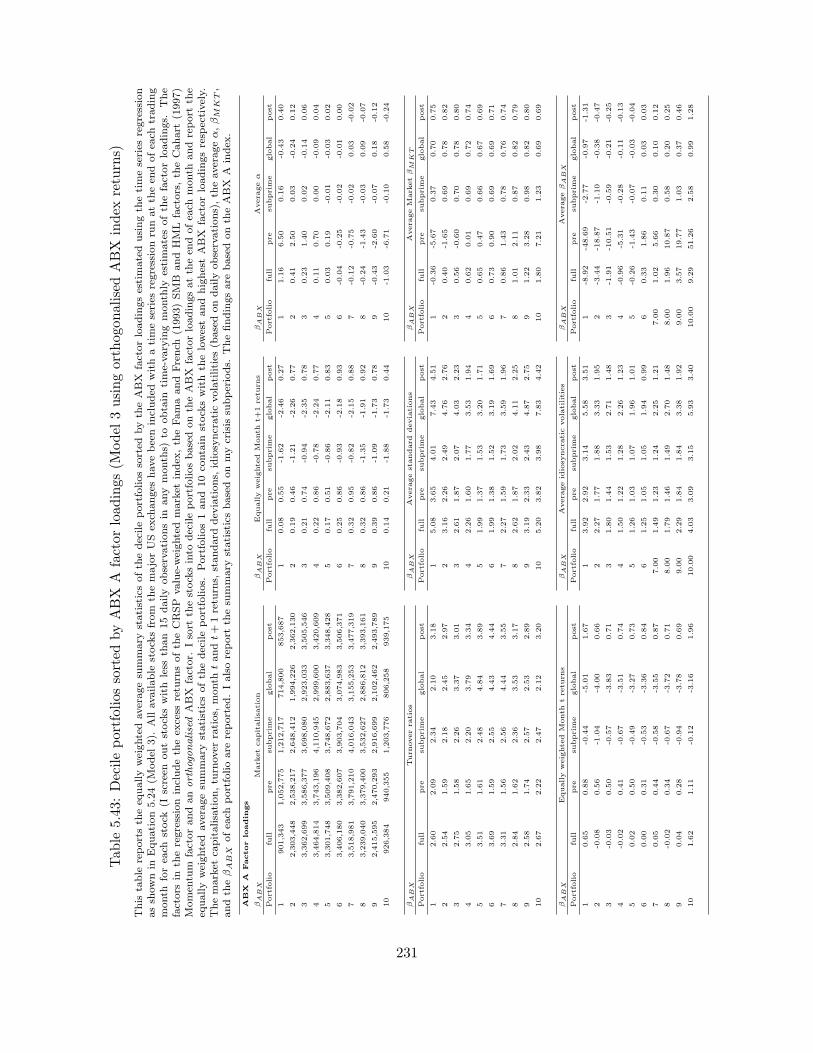
Tab
le5.43
:Decileportfoliossorted
byABX
Afactorloadings(M
odel
3usingorthogonalisedABX
index
returns)
This
table
reportsth
eeq
uallyweightedaveragesu
mmary
statisticsofth
edecileportfoliossorted
byth
eABX
factorloadingsestimatedusingth
etimeseries
regression
assh
ownin
Equation5.24(M
odel
3).
Allavailable
stock
sfrom
themajorUSex
changes
havebeenincluded
withatimeseries
regressionru
natth
een
dofea
chtrading
month
forea
chstock
(Iscreen
outstock
swith
less
than
15dailyobservationsin
anymonth
s)to
obtain
time-varyingmonth
lyestimatesofth
efactorloadings.
The
factors
inth
eregressionincludeth
eex
cess
retu
rnsofth
eCRSP
value-weightedmarket
index
,th
eFamaandFrench
(1993)SMB
andHML
factors,th
eCahart
(1997)
Momen
tum
factorandanorthogonalised
ABX
factor.
Isort
thestock
sinto
decileportfoliosbasedonth
eABX
factorloadingsatth
een
dofea
chmonth
andreport
the
equallyweightedaveragesu
mmary
statisticsofth
edecileportfolios.
Portfolios1and10co
ntain
stock
swithth
elowestandhighestABX
factorloadingsresp
ectively.
Themarket
capitalisation,tu
rnover
ratios,
month
tandt+
1retu
rns,
standard
dev
iations,
idiosyncraticvolatilities
(basedondailyobservations),th
eaverageα,βM
KT,
andth
eβABX
ofea
chportfolioare
reported
.Ialsoreport
thesu
mmary
statisticsbasedonmycrisis
subperiods.
Thefindingsare
basedonth
eABX
Aindex
.
ABX
AFactor
loadin
gs
βA
BX
Mark
etcapitalisa
tion
βA
BX
Equally
weighte
dM
onth
t+1
retu
rns
βA
BX
Avera
geα
Portfolio
full
pre
subprim
eglobal
post
Portfolio
full
pre
subprim
eglobal
post
Portfolio
full
pre
subprim
eglobal
post
1901,343
1,052,775
1,212,717
714,800
853,687
10.08
0.55
-1.62
-2.46
0.27
11.16
6.50
0.16
-0.43
0.40
22,303,448
2,538,217
2,648,412
1,994,226
2,362,130
20.19
0.46
-1.21
-2.26
0.77
20.41
2.50
0.03
-0.24
0.12
33,362,699
3,586,377
3,698,080
2,923,033
3,505,546
30.21
0.74
-0.94
-2.35
0.78
30.23
1.40
0.02
-0.14
0.06
43,464,814
3,743,196
4,110,945
2,999,600
3,420,609
40.22
0.86
-0.78
-2.24
0.77
40.11
0.70
0.00
-0.09
0.04
53,301,748
3,509,408
3,748,672
2,883,637
3,348,428
50.17
0.51
-0.86
-2.11
0.83
50.03
0.19
-0.01
-0.03
0.02
63,406,180
3,382,607
3,903,704
3,074,983
3,506,371
60.25
0.86
-0.93
-2.18
0.93
6-0
.04
-0.25
-0.02
-0.01
0.00
73,518,981
3,791,210
4,016,043
3,155,253
3,477,319
70.32
0.95
-0.82
-2.15
0.88
7-0
.12
-0.75
-0.02
0.03
-0.02
83,239,040
3,379,400
3,532,627
2,886,812
3,393,161
80.32
0.86
-1.35
-1.91
0.92
8-0
.24
-1.43
-0.03
0.09
-0.07
92,415,595
2,470,293
2,916,699
2,102,462
2,493,789
90.39
0.86
-1.09
-1.73
0.78
9-0
.43
-2.60
-0.07
0.18
-0.12
10
926,384
940,355
1,203,776
806,258
939,175
10
0.14
0.21
-1.88
-1.73
0.44
10
-1.03
-6.71
-0.10
0.58
-0.24
βA
BX
Turn
overra
tios
βA
BX
Avera
gestandard
deviations
βA
BX
Avera
geM
ark
etβM
KT
Portfolio
full
pre
subprim
eglobal
post
Portfolio
full
pre
subprim
eglobal
post
Portfolio
full
pre
subprim
eglobal
post
12.60
2.09
2.34
2.10
3.18
15.08
3.65
4.01
7.43
4.51
1-0
.36
-5.67
0.37
0.70
0.75
22.54
1.59
2.18
2.45
2.97
23.16
2.26
2.49
4.76
2.76
20.40
-1.65
0.69
0.78
0.82
32.75
1.58
2.26
3.37
3.01
32.61
1.87
2.07
4.03
2.23
30.56
-0.60
0.70
0.78
0.80
43.05
1.65
2.20
3.79
3.34
42.26
1.60
1.77
3.53
1.94
40.62
0.01
0.69
0.72
0.74
53.51
1.61
2.48
4.84
3.89
51.99
1.37
1.53
3.20
1.71
50.65
0.47
0.66
0.67
0.69
63.69
1.59
2.55
4.43
4.44
61.99
1.38
1.52
3.19
1.69
60.73
0.90
0.69
0.69
0.71
73.31
1.56
2.56
4.44
3.55
72.27
1.59
1.73
3.59
1.96
70.86
1.43
0.78
0.76
0.74
82.84
1.62
2.36
3.53
3.17
82.62
1.87
2.02
4.11
2.25
81.01
2.11
0.87
0.82
0.79
92.58
1.74
2.57
2.53
2.89
93.19
2.33
2.43
4.87
2.75
91.22
3.28
0.98
0.82
0.80
10
2.67
2.22
2.47
2.12
3.20
10
5.20
3.82
3.98
7.83
4.42
10
1.80
7.21
1.23
0.69
0.69
βA
BX
Equally
weighte
dM
onth
tre
turn
sβA
BX
Avera
geid
iosy
ncra
ticvolatilities
βA
BX
Avera
geβA
BX
Portfolio
full
pre
subprim
eglobal
post
Portfolio
full
pre
subprim
eglobal
post
Portfolio
full
pre
subprim
eglobal
post
10.65
0.88
-0.44
-5.01
1.67
13.92
2.92
3.14
5.58
3.51
1-8
.92
-48.69
-2.77
-0.97
-1.31
2-0
.08
0.56
-1.04
-4.00
0.66
22.27
1.77
1.88
3.33
1.95
2-3
.44
-18.87
-1.10
-0.38
-0.47
3-0
.03
0.50
-0.57
-3.83
0.71
31.80
1.44
1.53
2.71
1.48
3-1
.91
-10.51
-0.59
-0.21
-0.25
4-0
.02
0.41
-0.67
-3.51
0.74
41.50
1.22
1.28
2.26
1.23
4-0
.96
-5.31
-0.28
-0.11
-0.13
50.02
0.50
-0.49
-3.27
0.73
51.26
1.03
1.07
1.96
1.01
5-0
.26
-1.43
-0.07
-0.03
-0.04
60.00
0.31
-0.53
-3.36
0.84
61.25
1.05
1.05
1.94
0.99
60.33
1.86
0.11
0.03
0.03
70.05
0.44
-0.58
-3.55
0.87
7.00
1.49
1.23
1.24
2.25
1.21
7.00
1.02
5.66
0.30
0.10
0.12
8-0
.02
0.34
-0.67
-3.72
0.71
8.00
1.79
1.46
1.49
2.70
1.48
8.00
1.96
10.87
0.58
0.20
0.25
90.04
0.28
-0.94
-3.78
0.69
9.00
2.29
1.84
1.84
3.38
1.92
9.00
3.57
19.77
1.03
0.37
0.46
10
1.62
1.11
-0.12
-3.16
1.96
10.00
4.03
3.09
3.15
5.93
3.40
10.00
9.29
51.26
2.58
0.99
1.28
231
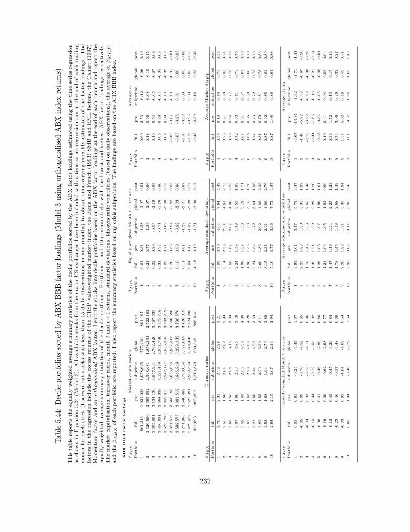
Tab
le5.44
:Decileportfoliossorted
byABX
BBB
factorloadings(M
odel
3usingorthogonalisedABX
index
returns)
This
table
reportsth
eeq
uallyweightedaveragesu
mmary
statisticsofth
edecileportfoliossorted
byth
eABX
factorloadingsestimatedusingth
etimeseries
regression
assh
ownin
Equation5.24(M
odel
3).
Allavailable
stock
sfrom
themajorUSex
changes
havebeenincluded
withatimeseries
regressionru
natth
een
dofea
chtrading
month
forea
chstock
(Iscreen
outstock
swith
less
than
15dailyobservationsin
anymonth
s)to
obtain
time-varyingmonth
lyestimatesofth
efactorloadings.
The
factors
inth
eregressionincludeth
eex
cess
retu
rnsofth
eCRSP
value-weightedmarket
index
,th
eFamaandFrench
(1993)SMB
andHML
factors,th
eCahart
(1997)
Momen
tum
factorandanorthogonalised
ABX
factor.
Isort
thestock
sinto
decileportfoliosbasedonth
eABX
factorloadingsatth
een
dofea
chmonth
andreport
the
equallyweightedaveragesu
mmary
statisticsofth
edecileportfolios.
Portfolios1and10co
ntain
stock
swithth
elowestandhighestABX
factorloadingsresp
ectively.
Themarket
capitalisation,tu
rnover
ratios,
month
tandt+
1retu
rns,
standard
dev
iations,
idiosyncraticvolatilities
(basedondailyobservations),th
eaverageα,βM
KT,
andth
eβABX
ofea
chportfolioare
reported
.Ialsoreport
thesu
mmary
statisticsbasedonmycrisis
subperiods.
Thefindingsare
basedonth
eABX
BBB
index
.
ABX
BBB
Factor
loadin
gs
βA
BX
Mark
etcapitalisa
tion
βA
BX
Equally
weighte
dM
onth
t+1
retu
rns
βA
BX
Avera
geα
Portfolio
full
pre
subprim
eglobal
post
Portfolio
full
pre
subprim
eglobal
post
Portfolio
full
pre
subprim
eglobal
post
1861,215
1,021,023
1,058,625
777,460
801,197
10.01
0.31
-1.58
-2.07
0.51
10.60
2.53
-0.12
-0.06
0.49
22,320,590
2,395,652
2,568,681
1,858,331
2,522,183
20.21
0.77
-1.39
-2.07
0.96
20.18
0.96
-0.08
-0.10
0.15
33,305,891
3,134,130
3,957,931
2,762,420
3,467,635
30.22
0.86
-0.95
-2.19
0.85
30.10
0.54
-0.05
-0.07
0.08
43,456,631
3,564,038
4,121,466
2,951,790
3,475,718
40.31
0.94
-0.71
-1.76
0.80
40.05
0.28
-0.04
-0.05
0.05
53,523,790
3,852,815
3,942,177
3,055,395
3,483,219
50.09
0.71
-0.69
-2.38
0.75
50.02
0.09
-0.01
-0.02
0.02
63,321,512
3,668,198
3,636,655
2,837,315
3,386,686
60.20
0.83
-0.94
-1.82
0.83
6-0
.02
-0.07
-0.01
-0.01
-0.01
73,588,575
3,691,512
3,845,848
3,228,133
3,700,570
70.16
0.98
-0.82
-2.33
0.86
7-0
.05
-0.25
0.01
0.00
-0.03
83,271,985
3,546,482
3,703,054
3,121,619
3,126,019
80.11
0.81
-1.32
-2.21
0.87
8-0
.10
-0.52
0.03
0.03
-0.08
92,429,622
2,522,391
2,962,369
2,148,445
2,424,205
90.04
0.47
-1.37
-2.28
0.77
9-0
.19
-0.93
0.03
0.05
-0.15
10
925,693
996,299
1,219,379
800,545
896,514
10
-0.18
0.19
-1.71
-2.00
0.17
10
-0.43
-2.39
0.15
0.23
-0.33
βA
BX
Turn
overra
tios
βA
BX
Avera
gestandard
deviations
βA
BX
Avera
geM
ark
etβM
KT
Portfolio
full
pre
subprim
eglobal
post
Portfolio
full
pre
subprim
eglobal
post
Portfolio
full
pre
subprim
eglobal
post
12.70
2.31
2.38
2.27
3.21
15.09
3.76
4.04
7.64
4.49
10.55
0.18
0.78
0.75
0.55
22.55
1.66
2.04
2.62
2.94
23.14
2.33
2.51
4.81
2.73
20.75
0.61
0.83
0.83
0.74
32.68
1.55
2.08
3.15
3.04
32.58
1.87
2.07
4.00
2.23
30.75
0.64
0.77
0.78
0.78
43.07
1.60
2.33
3.85
3.49
42.24
1.58
1.78
3.55
1.93
40.72
0.63
0.71
0.73
0.75
53.52
1.63
2.65
4.38
4.09
51.98
1.37
1.53
3.19
1.71
50.67
0.61
0.67
0.67
0.70
63.67
1.63
2.73
4.68
4.28
61.96
1.36
1.53
3.15
1.70
60.68
0.65
0.69
0.66
0.70
73.21
1.50
2.44
4.20
3.64
72.24
1.54
1.72
3.54
1.96
70.74
0.73
0.72
0.73
0.76
82.82
1.55
2.29
3.50
3.11
82.60
1.85
2.02
4.08
2.25
80.81
0.79
0.81
0.78
0.83
92.53
1.68
1.94
2.79
2.89
93.15
2.31
2.41
4.86
2.76
90.87
0.92
0.85
0.82
0.89
10
2.64
2.15
3.07
2.13
2.94
10
5.10
3.77
3.96
7.73
4.47
10
0.87
1.08
0.88
0.64
0.88
βA
BX
Equally
weighte
dM
onth
tre
turn
sβA
BX
Avera
geid
iosy
ncra
ticvolatilities
βA
BX
Avera
geβA
BX
Portfolio
full
pre
subprim
eglobal
post
Portfolio
full
pre
subprim
eglobal
post
Portfolio
full
pre
subprim
eglobal
post
10.53
0.61
-0.25
-4.49
1.67
13.93
3.01
3.17
5.73
3.47
1-3
.67
-14.81
-1.32
-1.71
-1.41
2-0
.35
0.09
-0.76
-4.52
0.85
22.25
1.82
1.90
3.35
1.92
2-1
.40
-5.72
-0.52
-0.67
-0.50
3-0
.24
0.33
-0.76
-4.11
0.96
31.76
1.45
1.53
2.65
1.46
3-0
.78
-3.22
-0.29
-0.38
-0.28
4-0
.15
0.34
-0.72
-3.55
0.92
41.49
1.21
1.29
2.29
1.20
4-0
.41
-1.66
-0.15
-0.21
-0.14
5-0
.06
0.41
-0.46
-2.99
0.86
51.26
1.03
1.07
1.96
1.01
5-0
.13
-0.54
-0.05
-0.08
-0.04
6-0
.16
0.39
-0.62
-2.98
0.77
61.24
1.03
1.05
1.92
0.99
60.10
0.41
0.04
0.03
0.04
7-0
.12
0.45
-0.45
-3.29
0.84
71.47
1.19
1.24
2.23
1.23
70.36
1.52
0.13
0.15
0.13
8-0
.23
0.46
-0.57
-3.48
0.66
81.78
1.45
1.48
2.68
1.49
80.74
3.06
0.26
0.32
0.27
9-0
.33
0.92
-1.04
-4.08
0.54
92.26
1.82
1.81
3.35
1.94
91.37
5.62
0.48
0.59
0.51
10
0.68
1.34
-0.40
-3.72
1.54
10
3.95
3.04
3.14
5.85
3.45
10
3.61
14.57
1.24
1.62
1.43
232

Tab
le5.45
:Decileportfoliossorted
byABX
BBB-factorloadings(M
odel
3usingorthogonalisedABX
index
returns)
This
table
reportsth
eeq
uallyweightedaveragesu
mmary
statisticsofth
edecileportfoliossorted
byth
eABX
factorloadingsestimatedusingth
etimeseries
regression
assh
ownin
Equation5.24(M
odel
3).
Allavailable
stock
sfrom
themajorUSex
changes
havebeenincluded
withatimeseries
regressionru
natth
een
dofea
chtrading
month
forea
chstock
(Iscreen
outstock
swith
less
than
15dailyobservationsin
anymonth
s)to
obtain
time-varyingmonth
lyestimatesofth
efactorloadings.
The
factors
inth
eregressionincludeth
eex
cess
retu
rnsofth
eCRSP
value-weightedmarket
index
,th
eFamaandFrench
(1993)SMB
andHML
factors,th
eCahart
(1997)
Momen
tum
factorandanorthogonalised
ABX
factor.
Isort
thestock
sinto
decileportfoliosbasedonth
eABX
factorloadingsatth
een
dofea
chmonth
andreport
the
equallyweightedaveragesu
mmary
statisticsofth
edecileportfolios.
Portfolios1and10co
ntain
stock
swithth
elowestandhighestABX
factorloadingsresp
ectively.
Themarket
capitalisation,tu
rnover
ratios,
month
tandt+
1retu
rns,
standard
dev
iations,
idiosyncraticvolatilities
(basedondailyobservations),th
eaverageα,βM
KT,
andth
eβABX
ofea
chportfolioare
reported
.Ialsoreport
thesu
mmary
statisticsbasedonmycrisis
subperiods.
Thefindingsare
basedonth
eABX
BBB-index
.
ABX
BBB-Factor
loadin
gs
βA
BX
Mark
etcapitalisa
tion
βA
BX
Equally
weighte
dM
onth
t+1
retu
rns
βA
BX
Avera
geα
Portfolio
full
pre
subprim
eglobal
post
Portfolio
full
pre
subprim
eglobal
post
Portfolio
full
pre
subprim
eglobal
post
1877,037
1,094,102
1,083,629
678,448
875,230
10.29
0.31
-1.90
-1.41
0.44
10.53
1.96
-0.20
-0.13
0.42
22,254,164
2,403,723
2,772,126
1,869,680
2,333,505
20.29
0.86
-1.13
-2.57
0.94
20.16
0.72
-0.10
-0.13
0.12
33,277,993
3,181,319
3,629,410
2,758,320
3,572,489
30.27
0.71
-0.99
-2.10
0.79
30.09
0.40
-0.06
-0.07
0.07
43,366,532
3,535,235
3,797,092
2,879,126
3,522,363
40.28
1.11
-0.82
-2.33
0.81
40.04
0.21
-0.05
-0.04
0.04
53,362,197
3,438,377
3,807,080
2,831,972
3,459,647
50.25
0.79
-0.75
-2.12
0.84
50.01
0.06
-0.03
-0.02
0.02
63,414,987
3,759,494
3,952,332
3,192,145
3,250,660
60.24
0.78
-0.73
-2.12
0.86
6-0
.01
-0.05
-0.01
-0.01
0.00
73,518,245
3,760,215
4,101,927
3,308,167
3,441,177
70.29
0.79
-0.92
-1.87
0.87
7-0
.04
-0.19
0.00
0.00
-0.03
83,366,317
3,422,941
3,732,308
3,017,521
3,462,629
80.25
0.73
-1.08
-2.08
0.84
8-0
.09
-0.39
0.02
0.04
-0.07
92,412,633
2,664,782
2,916,698
2,090,793
2,410,091
90.11
0.51
-1.32
-2.36
0.76
9-0
.16
-0.71
0.06
0.07
-0.13
10
989,577
1,117,823
1,210,139
910,771
971,258
10
0.02
0.28
-1.85
-2.15
0.21
10
-0.35
-1.77
0.22
0.26
-0.25
βA
BX
Turn
overra
tios
βA
BX
Avera
gestandard
deviations
βA
BX
Avera
geM
ark
etβM
KT
Portfolio
full
pre
subprim
eglobal
post
Portfolio
full
pre
subprim
eglobal
post
Portfolio
full
pre
subprim
eglobal
post
12.66
2.30
2.41
2.21
3.15
15.19
3.80
4.05
7.73
4.51
10.47
0.15
0.70
0.56
0.51
22.50
1.66
2.03
2.54
2.87
23.20
2.33
2.52
4.83
2.77
20.72
0.58
0.81
0.73
0.74
32.70
1.55
2.25
2.93
3.08
32.61
1.86
2.07
4.04
2.24
30.73
0.66
0.77
0.72
0.75
43.16
1.51
2.24
3.69
3.74
42.27
1.59
1.77
3.54
1.95
40.70
0.61
0.70
0.70
0.73
53.60
1.65
2.54
4.65
4.14
52.01
1.39
1.55
3.21
1.72
50.67
0.62
0.67
0.67
0.70
63.62
1.64
2.77
4.82
4.02
61.98
1.35
1.54
3.16
1.69
60.69
0.64
0.68
0.68
0.72
73.24
1.60
2.41
4.28
3.46
72.23
1.56
1.75
3.52
1.91
70.75
0.71
0.75
0.74
0.77
82.80
1.54
2.12
3.51
3.13
82.59
1.82
1.99
4.04
2.24
80.83
0.83
0.82
0.83
0.83
92.59
1.67
2.22
2.81
2.96
93.17
2.30
2.44
4.85
2.74
90.88
0.91
0.88
0.89
0.87
10
2.67
2.14
2.97
2.10
3.07
10
5.10
3.75
3.89
7.62
4.46
10
0.95
1.11
0.97
0.83
0.93
βA
BX
Equally
weighte
dM
onth
tre
turn
sβA
BX
Avera
geid
iosy
ncra
ticvolatilities
βA
BX
Avera
geβA
BX
Portfolio
full
pre
subprim
eglobal
post
Portfolio
full
pre
subprim
eglobal
post
Portfolio
full
pre
subprim
eglobal
post
10.73
0.77
-0.57
-5.09
1.71
14.00
3.05
3.19
5.80
3.48
1-3
.33
-11.54
-1.03
-1.60
-1.40
2-0
.14
0.00
-0.66
-4.40
0.61
22.31
1.83
1.92
3.38
1.94
2-1
.29
-4.49
-0.40
-0.64
-0.51
30.11
0.32
-0.47
-3.71
0.85
31.80
1.44
1.52
2.69
1.48
3-0
.71
-2.49
-0.22
-0.38
-0.28
40.07
0.42
-0.73
-3.30
0.81
41.51
1.22
1.28
2.29
1.22
4-0
.37
-1.28
-0.11
-0.22
-0.14
50.08
0.35
-0.59
-3.19
0.88
51.28
1.05
1.08
1.98
1.02
5-0
.13
-0.41
-0.03
-0.10
-0.04
60.10
0.49
-0.59
-3.06
0.86
61.25
1.02
1.06
1.91
0.99
60.08
0.32
0.03
0.01
0.03
70.05
0.58
-0.66
-3.36
0.85
71.47
1.20
1.26
2.22
1.19
70.32
1.18
0.11
0.12
0.13
8-0
.04
0.52
-0.78
-3.65
0.65
81.77
1.42
1.47
2.64
1.48
80.65
2.36
0.21
0.27
0.26
9-0
.01
0.56
-0.85
-3.81
0.58
92.26
1.81
1.84
3.33
1.91
91.21
4.32
0.38
0.52
0.49
10
1.28
1.34
-0.13
-3.61
1.81
10
3.94
3.01
3.06
5.75
3.45
10
3.27
11.18
0.98
1.41
1.39
233
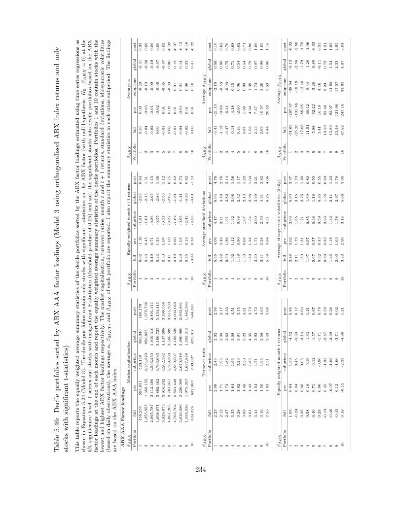
Tab
le5.46
:Decileportfoliossorted
byABX
AAA
factorloadings(M
odel
3usingorthogonalisedABX
index
returnsan
don
lystockswithsign
ificantt-statistics)
This
table
reportsth
eeq
uallyweightedaveragesu
mmary
statisticsofth
edecileportfoliossorted
byth
eABX
factorloadingsestimatedusingtimeseries
regressionsas
shownin
Equation5.24(M
odel
3).
Thedecileportfoliosco
ntain
only
stock
swithsignifica
ntt-statisticsonth
eABX
factor(w
ithnullhypoth
esis:H
0:βABX
=0)atth
e5%
significa
nce
level.Iscreen
outstock
swithinsignifica
ntF-statistics(thresh
old
p-valueof0.05)andsort
thesignifica
ntstock
sinto
decileportfoliosbasedonth
eABX
factorloadingsatth
een
dofea
chmonth
andreport
theeq
uallyweightedaveragesu
mmary
statisticsofth
edecileportfolios.
Portfolios1and10co
ntain
stock
swithth
elowestandhighestABX
factorloadingsresp
ectively.
Themarket
capitalisation,tu
rnover
ratios,
month
tandt+
1retu
rns,
standard
dev
iations,
idiosyncraticvolatilities
(basedondailyobservations),th
eaverageα,βM
KT,andβABX
ofea
chportfolioare
reported
.Ialsoreport
thesu
mmary
statisticsin
each
crisis
subperiod.Thefindings
are
basedonth
eABX
AAA
index
.
ABX
AA
AFactor
loadin
gs
βA
BX
Mark
etcapitalisa
tion
βA
BX
Equally
weighte
dm
onth
t+1
retu
rns
βA
BX
Avera
geα
Portfolio
full
pre
subprim
eglobal
post
Portfolio
full
pre
subprim
eglobal
post
Portfolio
full
pre
subprim
eglobal
post
1458,255
594,651
523,110
389,340
460,179
10.02
-1.16
-1.81
-2.93
0.84
10.10
0.03
-0.20
-0.31
0.33
21,355,555
1,358,155
2,154,320
856,038
1,375,798
20.43
0.45
-1.01
-2.15
1.31
2-0
.04
-0.03
-0.10
-0.36
0.09
32,895,787
3,112,486
4,596,250
1,919,310
2,891,111
30.19
0.71
-0.86
-2.95
1.15
3-0
.02
-0.01
-0.09
-0.19
0.06
44,608,071
3,882,462
6,703,693
3,166,725
5,134,411
40.33
1.33
-0.55
-2.83
1.36
40.00
-0.02
-0.06
-0.07
0.06
53,829,073
3,916,242
4,262,382
4,147,698
3,399,556
50.30
1.07
-0.37
-2.50
1.12
5-0
.01
0.01
-0.05
-0.07
0.02
64,061,205
3,761,857
5,769,360
3,565,899
3,815,333
60.11
1.03
-0.37
-2.66
0.75
60.00
0.02
-0.03
0.06
-0.02
74,762,704
5,851,448
4,960,507
4,169,539
4,603,060
70.19
0.60
-1.02
-1.31
0.42
7-0
.01
0.01
0.01
0.12
-0.07
83,026,586
3,226,099
2,670,218
3,090,999
2,903,891
80.49
1.05
-0.95
-1.41
0.73
8-0
.04
-0.01
0.01
0.14
-0.12
91,554,536
1,975,357
1,637,848
1,555,313
1,482,504
90.45
0.19
-2.43
-0.39
0.82
9-0
.02
0.01
0.08
0.23
-0.16
10
524,326
637,362
603,027
429,107
544,831
10
-0.34
0.33
-3.55
-0.01
-1.21
10
0.00
0.01
0.10
0.41
-0.22
βA
BX
Turn
overra
tio
βA
BX
Avera
gestandard
deviations
βA
BX
Avera
geβM
KT
Portfolio
full
pre
subprim
eglobal
post
Portfolio
full
pre
subprim
eglobal
post
Portfolio
full
pre
subprim
eglobal
post
12.23
2.08
2.43
2.02
2.36
15.45
4.06
4.17
8.04
4.76
1-3
.41
-21.13
-2.16
0.59
0.10
22.12
1.71
1.93
2.03
2.17
23.22
2.46
2.41
4.89
2.76
2-1
.13
-9.88
-0.53
0.80
0.62
32.27
1.72
1.82
2.62
2.32
32.50
1.86
1.91
3.82
2.14
3-0
.47
-6.44
-0.03
0.75
0.76
43.35
1.84
1.96
3.08
4.51
41.92
1.42
1.42
3.08
1.58
4-0
.14
-4.18
0.15
0.71
0.68
53.28
1.82
3.23
3.91
3.45
51.39
0.90
0.98
2.42
1.17
50.16
-2.00
0.36
0.54
0.62
63.69
1.48
2.50
5.23
4.21
61.33
0.68
1.07
2.13
1.22
60.87
1.80
0.93
0.54
0.71
73.61
1.43
1.86
4.35
3.79
71.89
1.24
1.54
2.98
1.64
71.58
4.94
1.39
0.79
0.90
83.41
1.54
1.71
3.93
4.72
82.50
1.71
2.00
3.90
2.21
82.13
7.47
1.74
0.97
1.06
93.16
1.50
1.95
2.58
4.63
93.21
2.28
2.56
4.91
2.82
92.69
10.57
2.20
0.99
1.05
10
2.55
1.83
2.31
2.43
3.00
10
5.38
3.84
4.31
8.25
4.66
10
4.44
20.62
3.53
0.86
1.16
βA
BX
Equally
weighte
dm
onth
tre
turn
sβA
BX
Avera
geid
iosy
ncra
ticvolatilities(d
aily)
βA
BX
Avera
geβA
BX
Portfolio
full
pre
subprim
eglobal
post
Portfolio
full
pre
subprim
eglobal
post
Portfolio
full
pre
subprim
eglobal
post
11.03
0.84
1.50
-4.52
0.85
13.88
3.02
3.03
5.63
3.37
1-5
1.69
-267.57
-38.64
-5.13
-6.02
2-0
.24
0.04
0.45
-5.33
0.17
22.11
1.79
1.65
3.15
1.73
2-2
5.26
-131.86
-18.18
-2.56
-2.80
30.25
0.30
0.03
-3.14
0.64
31.50
1.31
1.21
2.26
1.20
3-1
7.03
-88.95
-12.40
-1.79
-1.78
40.58
0.19
-0.19
-1.63
1.21
41.07
0.97
0.85
1.69
0.80
4-1
1.51
-60.42
-8.34
-1.28
-1.06
50.40
0.71
-0.12
-1.57
0.67
50.67
0.57
0.48
1.18
0.50
5-5
.88
-32.22
-3.28
-0.85
-0.33
60.28
0.66
-0.90
-1.71
0.79
60.62
0.43
0.59
0.85
0.55
63.41
16.18
4.16
-0.11
0.53
7-0
.13
0.45
-1.33
-2.87
0.59
70.99
0.83
0.96
1.38
0.83
710.20
52.48
8.24
0.72
1.21
8-0
.46
-0.07
-1.66
-2.99
0.28
81.46
1.18
1.32
2.11
1.23
815.89
82.07
11.92
1.54
1.95
9-0
.45
0.12
-1.60
-3.71
0.02
92.06
1.63
1.78
2.97
1.78
923.48
121.06
17.57
2.33
2.95
10
0.18
-0.55
-2.39
-4.06
1.21
10
3.83
2.90
3.14
5.66
3.30
10
47.82
247.16
34.93
4.87
6.04
234

Tab
le5.47:Decileportfoliossorted
byABX
AA
factorloadings(M
odel
3usingorthogonalisedABX
index
returnsandon
lystocks
withsign
ificantt-statistics)
This
table
reportsth
eeq
uallyweightedaveragesu
mmary
statisticsofth
edecileportfoliossorted
byth
eABX
factorloadingsestimated
usingtimeseries
regressionsas
shownin
Equation5.24(M
odel
3).
Thedecileportfoliosco
ntain
only
stock
swithsignifica
ntt-statisticsonth
eABX
factor(w
ithnullhypoth
esis:H
0:βABX
=0)atth
e5%
significa
nce
level.Iscreen
outstock
swithinsignifica
ntF-statistics(thresh
old
p-valueof0.05)andsort
thesignifica
ntstock
sinto
decileportfoliosbasedonth
eABX
factorloadingsatth
een
dofea
chmonth
andreport
theeq
uallyweightedaveragesu
mmary
statisticsofth
edecileportfolios.
Portfolios1and10co
ntain
stock
swithth
elowestandhighestABX
factorloadingsresp
ectively.
Themarket
capitalisation,tu
rnover
ratios,
month
tandt+
1retu
rns,
standard
dev
iations,
idiosyncraticvolatilities
(basedondailyobservations),th
eaverageα,βM
KT,andβABX
ofea
chportfolioare
reported
.Ialsoreport
thesu
mmary
statisticsin
each
crisis
subperiod.Thefindings
are
basedonth
eABX
AA
factor.
ABX
AA
Factor
loadin
gs
βA
BX
Mark
etcapitalisa
tion
βA
BX
Equally
weighte
dm
onth
t+1
retu
rns
βA
BX
Avera
geα
Portfolio
full
pre
subprim
eglobal
post
Portfolio
full
pre
subprim
eglobal
post
Portfolio
full
pre
subprim
eglobal
post
1482,109
464,442
574,337
378,924
545,356
10.72
-0.20
-2.13
-2.96
2.17
11.10
6.41
0.77
-1.01
0.38
21,312,073
1,521,307
1,826,571
746,782
1,391,180
20.49
1.13
-0.81
-2.57
1.20
20.49
3.22
0.37
-0.62
0.12
33,062,974
2,573,133
3,994,348
2,544,939
3,405,100
30.26
0.49
-0.38
-2.62
1.01
30.34
2.24
0.25
-0.44
0.09
44,724,368
4,148,932
6,720,699
3,299,724
5,377,184
40.28
0.64
-0.40
-2.78
1.22
40.26
1.62
0.12
-0.25
0.07
54,039,884
4,051,598
4,461,773
3,550,812
3,733,797
50.32
1.06
-0.21
-2.21
0.97
50.13
0.93
0.02
-0.17
0.03
64,523,437
5,717,479
4,988,746
5,078,645
3,949,126
60.17
0.99
-0.66
-1.84
0.65
6-0
.04
-0.08
-0.11
0.03
-0.03
74,485,887
5,774,962
4,994,242
3,440,579
4,265,299
70.35
1.26
-1.28
-2.00
1.15
7-0
.18
-1.03
-0.22
0.25
-0.09
83,571,893
3,794,547
3,853,915
3,285,937
3,769,407
80.47
1.52
-1.53
-1.64
0.77
8-0
.32
-1.79
-0.29
0.36
-0.14
91,401,676
1,624,154
1,518,574
1,377,190
1,407,365
90.28
0.40
-1.22
-1.81
0.70
9-0
.48
-2.70
-0.43
0.50
-0.20
10
510,793
672,129
658,038
446,015
442,494
10
-0.04
0.14
-3.07
-0.92
-0.11
10
-0.92
-5.49
-0.80
0.91
-0.32
βA
BX
Turn
overra
tio
βA
BX
Avera
gestandard
deviations
βA
BX
Avera
geβM
KT
Portfolio
full
pre
subprim
eglobal
post
Portfolio
full
pre
subprim
eglobal
post
Portfolio
full
pre
subprim
eglobal
post
12.23
1.99
2.13
2.18
2.34
15.41
4.13
4.36
7.86
4.70
1-2
.29
-14.79
-1.95
0.62
0.43
22.37
1.54
1.99
2.73
2.58
23.26
2.47
2.48
4.90
2.83
2-0
.64
-7.12
-0.37
0.75
0.76
32.26
1.56
1.92
2.20
2.49
32.50
1.89
1.96
3.72
2.14
3-0
.17
-4.66
0.01
0.76
0.80
43.11
1.59
2.34
4.26
3.14
41.94
1.46
1.48
3.10
1.58
40.06
-3.15
0.19
0.75
0.75
53.23
1.40
2.89
3.44
3.96
51.40
0.97
0.91
2.37
1.17
50.22
-1.56
0.28
0.58
0.61
64.07
1.60
3.03
5.20
4.27
61.31
0.77
1.00
2.07
1.18
60.68
0.86
0.84
0.56
0.61
73.48
1.46
2.28
4.38
3.78
71.87
1.10
1.50
3.11
1.63
71.27
3.26
1.35
0.81
0.81
83.65
1.32
5.66
2.88
4.24
82.49
1.61
1.95
3.94
2.17
81.72
5.13
1.77
0.87
0.97
92.23
1.59
2.00
2.45
2.29
93.22
2.25
2.55
4.85
2.84
92.12
7.39
2.09
0.87
1.00
10
2.58
2.06
2.40
2.31
3.08
10
5.44
3.82
4.25
8.35
4.72
10
3.23
14.11
3.36
0.56
0.86
βA
BX
Equally
weighte
dm
onth
tre
turn
sβA
BX
Avera
geid
iosy
ncra
ticvolatilities(d
aily)
βA
BX
Avera
geβA
BX
Portfolio
full
pre
subprim
eglobal
post
Portfolio
full
pre
subprim
eglobal
post
Portfolio
full
pre
subprim
eglobal
post
10.55
2.11
-0.07
-4.59
0.55
13.85
3.06
3.15
5.50
3.35
1-2
0.27
-101.56
-18.55
-2.08
-2.15
2-0
.28
-0.23
-0.20
-4.49
0.02
22.13
1.77
1.68
3.17
1.78
2-1
0.35
-52.78
-8.87
-1.07
-1.00
3-0
.12
-0.11
-0.15
-3.82
0.67
31.51
1.30
1.26
2.24
1.22
3-7
.13
-36.62
-6.01
-0.73
-0.64
40.36
0.47
-0.55
-2.19
1.12
41.06
0.99
0.88
1.66
0.79
4-5
.01
-26.14
-3.98
-0.51
-0.39
50.19
0.72
-0.42
-2.43
0.82
50.67
0.62
0.47
1.12
0.49
5-2
.64
-14.79
-1.47
-0.29
-0.08
60.45
0.80
-0.48
-2.42
1.38
60.60
0.45
0.54
0.84
0.52
60.67
1.56
1.94
0.09
0.20
7-0
.09
0.62
-1.18
-3.56
0.90
70.99
0.71
0.92
1.51
0.82
73.61
16.93
4.13
0.45
0.43
8-0
.22
0.35
-0.96
-3.80
0.72
81.46
1.09
1.28
2.18
1.22
86.00
29.04
6.25
0.69
0.67
9-0
.19
0.45
-1.63
-3.32
0.19
92.07
1.58
1.79
2.94
1.78
99.05
44.06
9.26
0.99
1.02
10
0.95
1.87
-2.60
-4.27
1.43
10
3.86
2.80
3.07
5.76
3.35
10
18.37
90.59
17.52
2.05
2.12
235

Tab
le5.48
:Decileportfoliossorted
byABX
Afactorloadings(M
odel
3usingorthogonalisedABX
index
returnsandon
lystocks
withsign
ificantt-statistics)
This
table
reportsth
eeq
uallyweightedaveragesu
mmary
statisticsofth
edecileportfoliossorted
byth
eABX
factorloadingsestimatedusingtimeseries
regressionsas
shownin
Equation5.24(M
odel
3).
Thedecileportfoliosco
ntain
only
stock
swithsignifica
ntt-statisticsonth
eABX
index
retu
rns(w
ithnullhypoth
esis:H
0:βABX
=0)
atth
e5%
significa
nce
level.Iscreen
outstock
swithinsignifica
ntF-statistics(thresh
old
p-valueof0.05)andsort
thesignifica
ntstock
sinto
decileportfoliosbasedonth
eABX
factorloadingsatth
een
dofea
chmonth
and
report
theeq
uallyweighted
averagesu
mmary
statisticsofth
edecileportfolios.
Portfolios1and
10co
ntain
stock
swithth
elowestandhighestABX
factorloadingsresp
ectively.
Themarket
capitalisation,tu
rnover
ratios,
month
tandt+
1retu
rns,
standard
dev
iations,
idiosyncratic
volatilities
(basedondailyobservations),th
eaverageα,βM
KT,andβABX
ofea
chportfolioare
reported
.Ialsoreport
thesu
mmary
statisticsin
each
crisis
subperiod.
Thefindingsare
basedonth
eABX
Aindex
.
ABX
AFactor
loadin
gs
βA
BX
Mark
etcapitalisa
tion
βA
BX
Equally
weighte
dm
onth
t+1
retu
rns
βA
BX
Avera
geα
Portfolio
full
pre
subprim
eglobal
post
Portfolio
full
pre
subprim
eglobal
post
Portfolio
full
pre
subprim
eglobal
post
1463,342
558,128
602,520
321,773
483,348
1-0
.75
1.08
-2.19
-3.83
-0.68
11.87
10.63
0.35
-0.69
0.58
21,397,902
1,461,084
1,874,690
1,035,292
1,467,169
20.43
0.74
-0.74
-2.83
1.03
20.86
5.31
0.11
-0.47
0.22
33,100,637
3,396,097
3,932,755
2,024,935
3,374,541
30.53
0.40
-0.18
-2.95
1.24
30.58
3.58
0.08
-0.30
0.15
44,635,680
4,861,828
5,230,183
3,286,063
5,265,817
40.21
0.34
-1.03
-2.57
1.39
40.38
2.36
0.05
-0.21
0.11
54,416,040
5,086,657
5,282,887
4,313,163
3,956,626
50.33
1.08
-0.04
-2.35
1.02
50.17
1.00
0.01
-0.10
0.06
64,264,319
3,913,970
4,684,306
3,787,506
4,656,860
60.23
0.88
-0.58
-1.76
0.69
6-0
.18
-1.08
-0.03
0.01
-0.02
74,937,474
5,226,155
5,534,866
4,326,436
4,955,386
70.35
1.14
-0.43
-2.06
0.84
7-0
.39
-2.46
-0.05
0.20
-0.10
83,174,891
2,391,990
4,030,437
2,885,376
3,306,389
80.48
0.62
-1.08
-1.32
1.36
8-0
.63
-3.80
-0.07
0.31
-0.19
91,475,906
1,642,244
1,927,725
1,449,857
1,288,586
90.68
0.24
-0.65
-0.99
1.06
9-0
.95
-5.65
-0.12
0.43
-0.30
10
518,852
426,689
769,296
484,748
512,527
10
-0.01
-0.76
-3.13
-1.37
0.40
10
-1.84
-11.41
-0.27
0.86
-0.47
βA
BX
Turn
overra
tio
βA
BX
Avera
gestandard
deviations
βA
BX
Avera
geβM
KT
Portfolio
full
pre
subprim
eglobal
post
Portfolio
full
pre
subprim
eglobal
post
Portfolio
full
pre
subprim
eglobal
post
12.15
2.06
2.28
2.19
2.25
15.40
3.88
4.42
8.01
4.71
1-1
.08
-9.63
0.14
0.69
0.68
22.12
1.55
2.21
2.38
2.13
23.23
2.36
2.61
4.90
2.77
2-0
.04
-4.37
0.56
0.79
0.86
32.91
1.30
2.04
2.73
3.52
32.51
1.77
2.08
3.87
2.11
30.25
-2.69
0.69
0.79
0.84
42.86
1.50
2.09
2.62
3.46
41.94
1.32
1.63
3.03
1.64
40.39
-1.49
0.68
0.69
0.79
54.32
1.73
4.77
5.98
4.05
51.37
0.85
1.07
2.32
1.17
50.44
-0.32
0.55
0.56
0.59
64.39
1.92
3.78
5.97
4.59
61.32
0.72
0.94
2.32
1.15
60.74
1.56
0.60
0.62
0.56
73.15
1.32
1.74
4.26
3.69
71.88
1.25
1.39
3.04
1.66
71.19
3.16
0.85
0.84
0.78
82.43
1.36
1.60
2.85
2.70
82.50
1.74
1.87
3.92
2.23
81.49
4.48
1.05
0.90
0.90
92.53
1.67
1.86
2.22
3.39
93.24
2.40
2.44
4.89
2.87
91.73
6.27
1.17
0.85
0.78
10
2.25
2.17
2.34
2.23
2.24
10
5.50
4.04
4.08
8.43
4.72
10
2.49
11.58
1.42
0.66
0.59
βA
BX
Equally
weighte
dm
onth
tre
turn
sβA
BX
Avera
geid
iosy
ncra
ticvolatilities(d
aily)
βA
BX
Avera
geβA
BX
Portfolio
full
pre
subprim
eglobal
post
Portfolio
full
pre
subprim
eglobal
post
Portfolio
full
pre
subprim
eglobal
post
10.94
0.68
0.86
-4.21
1.12
13.84
2.85
3.13
5.55
3.40
1-1
4.75
-80.02
-4.74
-1.66
-2.23
2-0
.58
-0.14
-0.28
-4.46
-0.10
22.11
1.66
1.79
3.13
1.76
2-7
.39
-40.31
-2.43
-0.83
-1.04
3-0
.06
0.14
-0.64
-2.92
0.47
31.52
1.21
1.35
2.29
1.22
3-5
.00
-27.29
-1.74
-0.56
-0.67
40.13
0.78
-0.12
-2.57
0.43
41.06
0.87
0.98
1.63
0.82
4-3
.29
-17.96
-1.19
-0.38
-0.42
50.39
0.87
-0.41
-2.19
1.05
50.64
0.50
0.56
1.08
0.48
5-1
.38
-7.58
-0.49
-0.18
-0.14
60.25
0.25
-0.62
-1.89
1.19
60.61
0.45
0.49
1.03
0.48
61.46
8.24
0.36
0.10
0.18
70.22
0.10
-1.25
-2.41
1.26
70.99
0.85
0.82
1.51
0.82
73.32
18.45
0.87
0.35
0.45
8-0
.02
0.42
-1.04
-3.12
0.99
81.47
1.22
1.19
2.22
1.24
85.17
28.73
1.37
0.55
0.71
90.31
0.19
-1.55
-2.31
0.89
92.09
1.72
1.66
3.06
1.82
97.72
42.84
2.00
0.81
1.09
10
1.39
1.36
-2.08
-4.14
2.51
10
3.94
3.04
2.97
5.92
3.35
10
15.73
87.07
3.97
1.68
2.26
236

Tab
le5.49
:Decileportfoliossorted
byABX
BBB
factorloadings(M
odel
3usingorthogonalisedABX
index
returnsan
don
lystockswithsign
ificantt-statistics)
This
table
reportsth
eeq
uallyweightedaveragesu
mmary
statisticsofth
edecileportfoliossorted
byth
eABX
factorloadingsestimatedusingtimeseries
regressionsas
shownin
Equation5.24(M
odel
3).
Thedecileportfoliosco
ntain
only
stock
swithsignifica
ntt-statisticsonth
eABX
index
retu
rns(w
ithnullhypoth
esis:H
0:βABX
=0)
atth
e5%
significa
nce
level.Iscreen
outstock
swithinsignifica
ntF-statistics(thresh
old
p-valueof0.05)andsort
thesignifica
ntstock
sinto
decileportfoliosbasedonth
eABX
factorloadingsatth
een
dofea
chmonth
andreport
theeq
uallyweightedaveragesu
mmary
statisticsofth
edecileportfolios.
Portfolios1and10co
ntain
stock
swithth
elowestandhighestABX
factorloadingsresp
ectively.
Themarket
capitalisation,tu
rnover
ratios,
month
tandt+
1retu
rns,
standard
dev
iations,
idiosyncratic
volatilities
(basedondailyobservations),th
eaverageα,βM
KT,andβABX
ofea
chportfolioare
reported
.Ialsoreport
thesu
mmary
statisticsin
each
crisis
subperiod.
Thefindingsare
basedonth
eABX
BBB
index
.
ABX
BBB
Factor
loadin
gs
βA
BX
Mark
etcapitalisa
tion
βA
BX
Equally
weighte
dm
onth
t+1
retu
rns
βA
BX
Avera
geα
Portfolio
full
pre
subprim
eglobal
post
Portfolio
full
pre
subprim
eglobal
post
Portfolio
full
pre
subprim
eglobal
post
1468,848
684,313
483,245
373,142
459,971
10.26
1.16
-1.97
-1.27
0.36
10.97
4.28
-0.09
-0.14
0.71
21,359,614
1,464,512
1,435,693
1,041,838
1,501,740
20.63
0.49
-0.50
-1.95
1.34
20.42
2.10
-0.12
-0.18
0.31
32,898,472
2,549,949
2,995,215
2,671,430
3,202,636
30.11
0.66
-1.00
-3.03
1.12
30.27
1.46
-0.11
-0.13
0.20
44,865,036
4,528,078
4,899,650
4,302,911
5,443,911
40.14
1.00
-1.20
-2.76
1.14
40.20
1.02
-0.08
-0.04
0.15
53,805,916
3,823,140
4,518,673
3,206,064
3,889,291
50.26
0.70
-0.27
-2.04
0.87
50.11
0.62
-0.03
-0.07
0.08
63,890,121
4,684,206
4,410,494
3,910,955
3,469,095
6-0
.32
0.79
-1.25
-2.81
0.32
6-0
.03
-0.14
-0.01
0.00
-0.01
75,082,641
4,807,112
6,133,315
4,340,383
5,360,079
70.05
0.80
-0.73
-1.62
0.33
7-0
.16
-0.81
0.04
0.06
-0.11
83,249,153
3,459,228
4,328,090
2,260,233
3,355,965
80.05
0.73
-1.59
-1.99
0.86
8-0
.28
-1.36
0.07
0.09
-0.21
91,479,879
1,201,431
2,024,986
1,286,693
1,555,917
90.25
0.90
-1.04
-1.99
0.74
9-0
.45
-2.08
0.08
0.07
-0.35
10
522,689
614,156
872,023
378,987
451,232
10
-0.18
-0.36
-1.93
-0.92
-0.23
10
-0.86
-4.18
0.14
0.18
-0.63
βA
BX
Turn
overra
tio
βA
BX
Avera
gestandard
deviations
βA
BX
Avera
geβM
KT
Portfolio
full
pre
subprim
eglobal
post
Portfolio
full
pre
subprim
eglobal
post
Portfolio
full
pre
subprim
eglobal
post
12.29
2.28
2.37
1.95
2.48
15.44
4.04
4.40
8.26
4.71
10.42
-0.18
0.81
0.82
0.38
22.14
1.66
1.88
2.57
2.19
23.25
2.37
2.60
5.03
2.82
20.73
0.42
0.86
0.90
0.71
32.47
1.68
2.11
2.77
2.77
32.52
1.86
2.05
4.02
2.12
30.80
0.61
0.89
0.86
0.80
42.83
1.31
2.21
3.63
3.07
41.93
1.43
1.56
3.14
1.58
40.76
0.73
0.79
0.76
0.76
53.61
1.50
2.27
4.73
4.44
51.41
0.93
1.07
2.33
1.21
50.60
0.50
0.57
0.53
0.68
64.57
1.64
5.20
5.86
4.92
61.32
0.67
0.96
2.28
1.20
60.61
0.58
0.57
0.53
0.65
73.22
1.49
1.99
4.58
3.53
71.79
1.14
1.39
2.95
1.54
70.77
0.85
0.74
0.74
0.76
82.43
1.34
1.87
3.29
2.55
82.44
1.69
1.86
3.90
2.13
80.92
1.05
0.88
0.86
0.91
93.81
1.82
8.90
1.87
3.58
93.16
2.36
2.41
4.85
2.78
90.96
1.24
0.87
0.78
0.97
10
2.20
2.02
2.21
2.02
2.45
10
5.30
4.05
4.07
8.01
4.67
10
0.89
1.27
0.80
0.50
0.96
βA
BX
Equally
weighte
dm
onth
tre
turn
sβA
BX
Avera
geid
iosy
ncra
ticvolatilities(d
aily)
βA
BX
Avera
geβA
BX
Portfolio
full
pre
subprim
eglobal
post
Portfolio
full
pre
subprim
eglobal
post
Portfolio
full
pre
subprim
eglobal
post
10.54
1.37
1.05
-3.41
0.33
13.87
2.94
3.13
5.74
3.38
1-6
.19
-24.73
-2.28
-2.86
-2.46
2-0
.44
0.34
-0.41
-5.38
0.48
22.10
1.66
1.77
3.15
1.77
2-3
.06
-12.51
-1.14
-1.49
-1.11
3-0
.58
-0.29
-0.86
-4.40
0.53
31.49
1.26
1.32
2.31
1.18
3-2
.12
-8.85
-0.79
-1.02
-0.71
4-0
.05
0.13
-0.24
-3.26
0.99
41.05
0.92
0.95
1.65
0.80
4-1
.46
-6.25
-0.55
-0.70
-0.45
50.05
0.43
-0.49
-2.21
0.72
50.66
0.59
0.58
1.10
0.47
5-0
.82
-3.72
-0.27
-0.36
-0.19
60.02
0.52
-0.56
-2.47
0.98
60.57
0.39
0.49
0.97
0.44
60.20
0.73
0.13
0.06
0.09
7-0
.15
0.56
-0.87
-2.41
0.78
70.94
0.75
0.83
1.42
0.76
71.15
4.79
0.45
0.47
0.43
8-0
.31
0.54
-0.80
-2.93
0.48
81.41
1.15
1.17
2.12
1.18
81.94
8.03
0.69
0.85
0.72
9-0
.43
0.41
-1.06
-3.62
0.34
92.03
1.64
1.60
3.02
1.74
92.95
12.23
1.00
1.28
1.13
10
-0.65
0.53
-1.61
-6.16
0.77
10
3.80
3.03
2.96
5.63
3.32
10
6.10
24.97
2.05
2.66
2.42
237

Tab
le5.50
:Decileportfoliossorted
byABX
BBB-factorloadings(M
odel
3usingorthogonalisedABX
index
returnsan
don
lystockswithsign
ificantt-statistics)
This
table
reportsth
eeq
uallyweightedaveragesu
mmary
statisticsofth
edecileportfoliossorted
byth
eABX
factorloadingsestimatedusingtimeseries
regressionsas
shownin
Equation5.24(M
odel
3).
Thedecileportfoliosco
ntain
only
stock
swithsignifica
ntt-statisticsonth
eABX
index
retu
rns(w
ithnullhypoth
esis:H
0:βABX
=0)
atth
e5%
significa
nce
level.Iscreen
outstock
swithinsignifica
ntF-statistics(thresh
old
p-valueof0.05)andsort
thesignifica
ntstock
sinto
decileportfoliosbasedon
theABX
factorloadingsatth
een
dofea
chmonth
andreport
theeq
uallyweightedaveragesu
mmary
statisticsofth
edecileportfolios.
Portfolios1and10co
ntain
stock
swithth
elowestandhighestABX
factorloadingsresp
ectively.
Themarket
capitalisation,tu
rnover
ratios,
month
tandt+
1retu
rns,
standard
dev
iations,
idiosyncratic
volatilities
(basedondailyobservations),th
eaverageα,βM
KT,andβABX
ofea
chportfolioare
reported
.Ialsoreport
thesu
mmary
statisticsin
each
crisis
subperiod.
Thefindingsare
basedonth
eABX
BBB-index
.
ABX
BBB-Factor
loadin
gs
βA
BX
Mark
etcapitalisa
tion
βA
BX
Equally
weighte
dm
onth
t+1
retu
rns
βA
BX
Avera
geα
Portfolio
full
pre
subprim
eglobal
post
Portfolio
full
pre
subprim
eglobal
post
Portfolio
full
pre
subprim
eglobal
post
1450,032
672,592
481,767
269,206
473,188
10.10
-0.30
-2.06
-1.55
-0.14
10.81
3.40
-0.32
-0.28
0.61
21,373,887
1,548,570
1,725,058
1,111,383
1,374,855
20.35
-0.16
-0.56
-2.11
0.71
20.34
1.62
-0.18
-0.22
0.26
32,666,409
3,220,321
3,202,063
2,001,897
2,748,625
30.46
0.84
-0.81
-2.69
1.39
30.21
1.09
-0.15
-0.20
0.17
44,664,202
4,758,937
5,606,494
4,265,124
4,751,363
40.45
0.93
-0.73
-2.09
1.24
40.15
0.76
-0.13
-0.09
0.12
53,774,628
4,230,124
4,397,050
2,742,342
4,067,308
50.31
0.89
-0.43
-1.91
0.78
50.08
0.41
-0.07
-0.06
0.08
64,155,540
4,438,993
4,629,812
4,415,023
3,931,687
60.34
0.82
-0.44
-2.15
1.19
6-0
.05
-0.23
0.01
-0.03
-0.01
74,395,648
4,881,536
6,088,836
3,572,490
4,137,529
70.18
0.41
-1.25
-2.52
1.37
7-0
.13
-0.69
0.05
0.12
-0.09
83,378,400
3,007,345
4,334,317
2,949,251
3,487,893
80.23
1.01
-1.03
-1.91
0.80
8-0
.22
-1.02
0.08
0.13
-0.19
91,667,587
1,864,797
1,851,382
1,435,427
1,790,165
90.46
0.98
-0.43
-2.65
1.20
9-0
.34
-1.52
0.13
0.11
-0.24
10
496,454
553,783
692,360
449,970
444,150
10
-0.52
-0.95
-1.76
-2.47
-0.05
10
-0.73
-3.16
0.21
0.30
-0.56
βA
BX
Turn
overra
tio
βA
BX
Avera
gestandard
deviations
βA
BX
Avera
geβM
KT
Portfolio
full
pre
subprim
eglobal
post
Portfolio
full
pre
subprim
eglobal
post
Portfolio
full
pre
subprim
eglobal
post
12.90
2.23
2.27
1.64
4.20
15.55
4.14
4.41
8.32
4.71
10.26
-0.28
0.68
0.36
0.37
22.27
1.87
1.74
2.23
2.65
23.33
2.36
2.57
5.14
2.88
20.67
0.41
0.77
0.71
0.71
32.30
1.62
2.15
2.30
2.53
32.60
1.80
2.04
4.06
2.24
30.77
0.55
0.88
0.78
0.81
42.84
1.27
2.51
2.77
3.47
42.03
1.38
1.59
3.22
1.73
40.72
0.63
0.75
0.72
0.75
53.42
1.73
2.86
3.79
4.01
51.45
0.88
1.05
2.43
1.25
50.58
0.53
0.64
0.52
0.58
64.69
1.87
7.39
5.71
4.07
61.29
0.67
0.95
2.21
1.14
60.61
0.61
0.60
0.53
0.62
73.61
1.49
1.97
5.90
3.55
71.76
1.24
1.40
2.75
1.55
70.82
0.98
0.77
0.79
0.80
82.43
1.54
1.73
2.73
2.83
82.41
1.74
1.84
3.74
2.08
80.98
1.12
0.91
0.97
0.95
93.22
1.73
7.11
2.44
2.68
93.12
2.28
2.42
4.71
2.73
91.03
1.26
1.00
0.94
1.00
10
2.37
2.00
2.33
1.74
2.94
10
5.29
4.04
4.09
7.87
4.60
10
1.09
1.52
1.07
0.93
1.00
βA
BX
Equally
weighte
dm
onth
tre
turn
sβA
BX
Avera
geid
iosy
ncra
ticvolatilities(d
aily)
βA
BX
Avera
geβA
BX
Portfolio
full
pre
subprim
eglobal
post
Portfolio
full
pre
subprim
eglobal
post
Portfolio
full
pre
subprim
eglobal
post
10.10
1.51
-0.46
-5.30
0.41
13.96
3.03
3.17
5.86
3.34
1-5
.58
-19.71
-1.78
-2.70
-2.39
2-0
.42
-0.05
-0.50
-5.23
0.31
22.18
1.66
1.77
3.27
1.83
2-2
.74
-9.85
-0.89
-1.34
-1.16
3-0
.32
-0.07
-0.79
-4.70
0.78
31.57
1.22
1.32
2.41
1.28
3-1
.85
-6.71
-0.62
-0.94
-0.77
40.11
0.36
-0.55
-3.39
0.97
41.13
0.92
0.97
1.75
0.88
4-1
.27
-4.67
-0.44
-0.67
-0.51
50.30
0.55
-0.38
-2.44
0.99
50.70
0.55
0.56
1.18
0.52
5-0
.68
-2.51
-0.21
-0.41
-0.24
60.06
0.42
-0.33
-3.00
0.89
60.57
0.39
0.49
0.96
0.45
60.25
1.22
0.12
-0.11
0.11
70.05
0.66
-0.91
-2.14
0.69
70.92
0.81
0.84
1.29
0.75
71.03
4.12
0.33
0.33
0.42
80.01
1.12
-0.86
-3.03
0.53
81.41
1.17
1.17
2.05
1.18
81.68
6.36
0.53
0.71
0.70
90.04
1.20
-1.01
-3.97
0.97
92.00
1.57
1.63
2.91
1.71
92.56
9.46
0.77
1.11
1.09
10
0.01
0.60
-1.22
-5.21
0.46
10
3.76
2.98
2.95
5.47
3.25
10
5.46
19.34
1.55
2.31
2.38
238
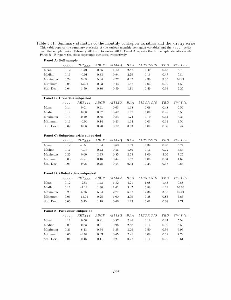
Table 5.51: Summary statistics of the monthly contagion variables and the κAAA,t seriesThis table reports the summary statistics of the various monthly contagion variables and the κAAA,t seriesover the sample period February 2006 to December 2011. Panel A reports the full sample statistics whilePanel B - E report the crisis subsample statistics, respectively.
Panel A: Full sample
κAAA,t RETAAA ABCP AILLIQ BAA LIBOR-OIS TED VW IV ol
Mean 0.12 -0.21 0.65 1.10 2.87 0.40 0.66 6.70
Median 0.11 -0.01 0.33 0.94 2.79 0.16 0.47 5.84
Maximum 0.29 9.63 5.04 2.77 6.07 2.36 3.15 16.21
Minimum 0.05 -15.01 0.03 0.43 1.57 0.03 0.12 4.50
Std. Dev. 0.04 3.50 0.80 0.59 1.11 0.49 0.61 2.25
Panel B: Pre-crisis subperiod
κAAA,t RETAAA ABCP AILLIQ BAA LIBOR-OIS TED VW IV ol
Mean 0.14 0.01 0.41 0.63 1.68 0.08 0.48 5.56
Median 0.14 0.00 0.37 0.62 1.67 0.09 0.48 5.50
Maximum 0.16 0.19 0.88 0.83 1.74 0.10 0.61 6.34
Minimum 0.11 -0.06 0.14 0.43 1.64 0.03 0.31 4.50
Std. Dev. 0.02 0.06 0.26 0.12 0.03 0.02 0.08 0.47
Panel C: Subprime crisis subperiod
κAAA,t RETAAA ABCP AILLIQ BAA LIBOR-OIS TED VW IV ol
Mean 0.12 -0.56 1.04 0.60 1.89 0.34 0.95 5.74
Median 0.11 -0.13 0.73 0.56 1.80 0.11 0.72 5.53
Maximum 0.25 0.60 2.23 0.85 2.53 1.00 2.05 7.25
Minimum 0.08 -2.40 0.16 0.44 1.57 0.08 0.34 4.69
Std. Dev. 0.05 0.98 0.78 0.14 0.33 0.34 0.58 0.85
Panel D: Global crisis subperiod
κAAA,t RETAAA ABCP AILLIQ BAA LIBOR-OIS TED VW IV ol
Mean 0.12 -2.54 1.43 1.82 4.21 1.08 1.43 9.88
Median 0.11 -2.14 1.30 1.61 3.47 0.88 1.19 10.00
Maximum 0.29 5.76 5.04 2.77 6.07 2.36 3.15 16.21
Minimum 0.05 -15.01 0.25 1.00 2.99 0.38 0.83 6.63
Std. Dev. 0.06 5.45 1.18 0.66 1.23 0.61 0.68 2.71
Panel E: Post-crisis subperiod
κAAA,t RETAAA ABCP AILLIQ BAA LIBOR-OIS TED VW IV ol
Mean 0.11 0.56 0.21 0.97 2.86 0.19 0.24 5.59
Median 0.09 0.63 0.21 0.96 2.88 0.14 0.19 5.50
Maximum 0.21 6.43 0.54 1.35 3.29 0.50 0.56 6.95
Minimum 0.06 -3.94 0.03 0.65 2.41 0.09 0.12 4.79
Std. Dev. 0.04 2.46 0.11 0.21 0.27 0.11 0.12 0.61
239
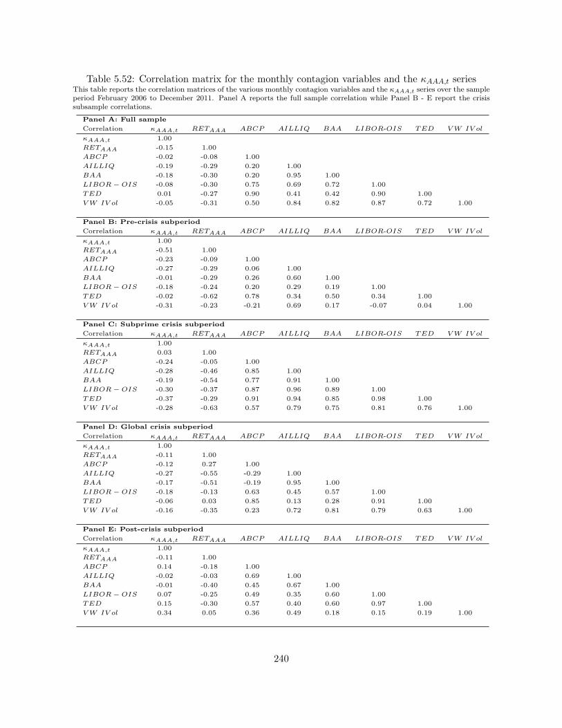
Table 5.52: Correlation matrix for the monthly contagion variables and the κAAA,t seriesThis table reports the correlation matrices of the various monthly contagion variables and the κAAA,t series over the sampleperiod February 2006 to December 2011. Panel A reports the full sample correlation while Panel B - E report the crisissubsample correlations.
Panel A: Full sample
Correlation κAAA,t RETAAA ABCP AILLIQ BAA LIBOR-OIS TED V W IV ol
κAAA,t 1.00
RETAAA -0.15 1.00
ABCP -0.02 -0.08 1.00
AILLIQ -0.19 -0.29 0.20 1.00
BAA -0.18 -0.30 0.20 0.95 1.00
LIBOR − OIS -0.08 -0.30 0.75 0.69 0.72 1.00
TED 0.01 -0.27 0.90 0.41 0.42 0.90 1.00
V W IV ol -0.05 -0.31 0.50 0.84 0.82 0.87 0.72 1.00
Panel B: Pre-crisis subperiod
Correlation κAAA,t RETAAA ABCP AILLIQ BAA LIBOR-OIS TED V W IV ol
κAAA,t 1.00
RETAAA -0.51 1.00
ABCP -0.23 -0.09 1.00
AILLIQ -0.27 -0.29 0.06 1.00
BAA -0.01 -0.29 0.26 0.60 1.00
LIBOR − OIS -0.18 -0.24 0.20 0.29 0.19 1.00
TED -0.02 -0.62 0.78 0.34 0.50 0.34 1.00
V W IV ol -0.31 -0.23 -0.21 0.69 0.17 -0.07 0.04 1.00
Panel C: Subprime crisis subperiod
Correlation κAAA,t RETAAA ABCP AILLIQ BAA LIBOR-OIS TED V W IV ol
κAAA,t 1.00
RETAAA 0.03 1.00
ABCP -0.24 -0.05 1.00
AILLIQ -0.28 -0.46 0.85 1.00
BAA -0.19 -0.54 0.77 0.91 1.00
LIBOR − OIS -0.30 -0.37 0.87 0.96 0.89 1.00
TED -0.37 -0.29 0.91 0.94 0.85 0.98 1.00
V W IV ol -0.28 -0.63 0.57 0.79 0.75 0.81 0.76 1.00
Panel D: Global crisis subperiod
Correlation κAAA,t RETAAA ABCP AILLIQ BAA LIBOR-OIS TED V W IV ol
κAAA,t 1.00
RETAAA -0.11 1.00
ABCP -0.12 0.27 1.00
AILLIQ -0.27 -0.55 -0.29 1.00
BAA -0.17 -0.51 -0.19 0.95 1.00
LIBOR − OIS -0.18 -0.13 0.63 0.45 0.57 1.00
TED -0.06 0.03 0.85 0.13 0.28 0.91 1.00
V W IV ol -0.16 -0.35 0.23 0.72 0.81 0.79 0.63 1.00
Panel E: Post-crisis subperiod
Correlation κAAA,t RETAAA ABCP AILLIQ BAA LIBOR-OIS TED V W IV ol
κAAA,t 1.00
RETAAA -0.11 1.00
ABCP 0.14 -0.18 1.00
AILLIQ -0.02 -0.03 0.69 1.00
BAA -0.01 -0.40 0.45 0.67 1.00
LIBOR − OIS 0.07 -0.25 0.49 0.35 0.60 1.00
TED 0.15 -0.30 0.57 0.40 0.60 0.97 1.00
V W IV ol 0.34 0.05 0.36 0.49 0.18 0.15 0.19 1.00
240
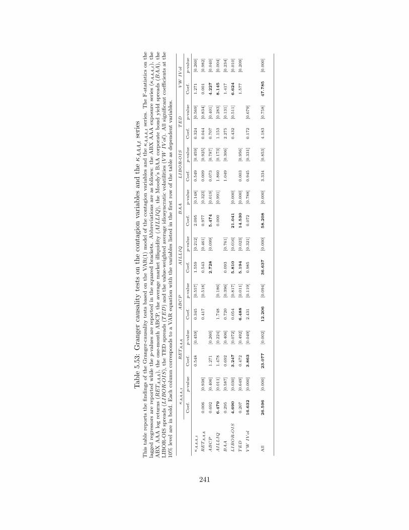
Tab
le5.53
:Granger
causality
testsonthecontagionvariablesandtheκAAA,tseries
This
table
reportsth
efindingsofth
eGranger-causality
testsbasedonth
eVAR(1)model
ofth
eco
ntagionvariablesandth
eκAAA,t
series.TheF-statisticsonth
elagged
regressors
are
reported
whileth
ep-values
are
reported
inth
esquaredbrackets.
Abbreviationsare
asfollows:
theABX
AAA
exposu
reseries
(κAAA,t),
the
ABX
AAA
logretu
rns(R
ETAAA),
theone-month
ABCP,th
eaveragemarket
illiquidity(A
ILLIQ),
theMoody’s
BAA
corp
orate
bondyield
spreads(B
AA),
the
LIB
OR-O
ISsp
reads(L
IBOR-O
IS),
theTED
spreads(T
ED)andth
evalue-weightedaverageidiosyncraticvolatilities
(VW
IVol).Allsignifica
ntco
efficien
tsatth
e10%
level
are
inbold.Each
columnco
rrespondsto
aVAR
equationwithth
evariableslisted
inth
efirstrow
ofth
etable
asdep
enden
tvariables.
κA
AA
,tRETA
AA
ABCP
AILLIQ
BAA
LIBOR-O
IS
TED
VW
IVol
Coef.
p-valu
eCoef.
p-valu
eCoef.
p-valu
eCoef.
p-valu
eCoef.
p-valu
eCoef.
p-valu
eCoef.
p-valu
eCoef.
p-valu
e
κA
AA
,t0.548
[0.459]
0.345
[0.557]
1.559
[0.212]
2.095
[0.148]
0.549
[0.459]
0.324
[0.569]
1.271
[0.260]
RETA
AA
0.006
[0.938]
0.417
[0.518]
0.543
[0.461]
0.977
[0.323]
0.009
[0.925]
0.044
[0.834]
0.001
[0.982]
ABCP
0.692
[0.406]
1.271
[0.260]
2.7
28
[0.099]
5.4
74
[0.019]
0.073
[0.787]
0.707
[0.401]
4.2
27
[0.040]
AILLIQ
6.4
79
[0.011]
1.478
[0.224]
1.748
[0.186]
0.000
[0.991]
1.860
[0.173]
1.153
[0.283]
8.1
45
[0.004]
BAA
0.295
[0.587]
0.692
[0.406]
0.720
[0.396]
0.093
[0.761]
1.049
[0.306]
2.275
[0.131]
1.417
[0.234]
LIBOR-O
IS
4.6
90
[0.030]
3.2
47
[0.072]
0.054
[0.817]
5.8
10
[0.016]
21.0
41
[0.000]
0.432
[0.511]
6.6
24
[0.010]
TED
0.207
[0.649]
0.472
[0.492]
6.4
88
[0.011]
5.1
94
[0.023]
14.5
30
[0.000]
0.003
[0.956]
1.577
[0.209]
VW
IVol
16.6
32
[0.000]
3.8
63
[0.049]
2.431
[0.119]
0.985
[0.321]
0.072
[0.788]
0.945
[0.331]
0.172
[0.679]
All
26.5
96
[0.000]
23.0
77
[0.002]
12.2
06
[0.094]
36.6
37
[0.000]
58.2
08
[0.000]
3.334
[0.853]
4.183
[0.758]
47.7
85
[0.000]
241
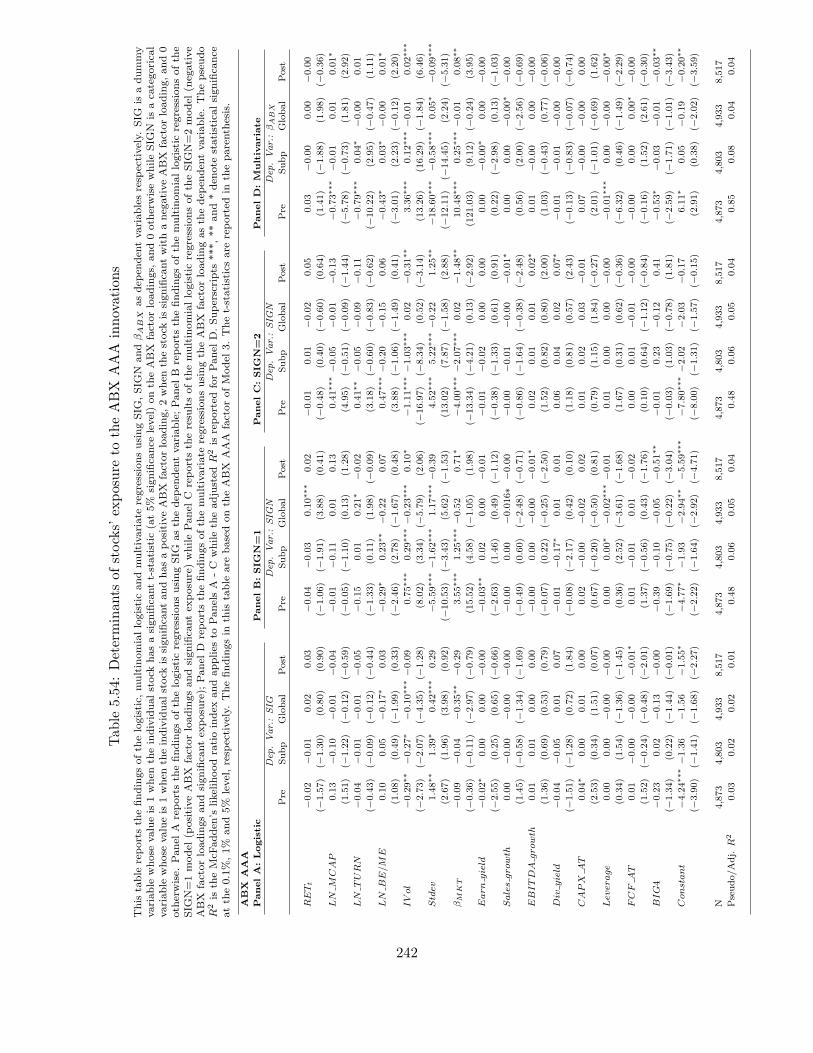
Tab
le5.54
:Determinants
ofstocks’
exposure
totheABX
AAA
innovations
This
table
reportsth
efindingsofth
elogistic,
multinomiallogisticandmultivariate
regressionsusingSIG
,SIG
NandβABX
asdep
enden
tvariablesresp
ectively.
SIG
isadummy
variable
whose
valueis
1when
theindividualstock
hasasignifica
ntt-statistic
(at5%
significa
nce
level)onth
eABX
factorloadings,
and0oth
erwisewhileSIG
Nis
aca
tegorica
lvariable
whose
valueis
1when
theindividualstock
issignifica
ntandhasapositiveABX
factorloading,2when
thestock
issignifica
ntwithaneg
ativeABX
factorloading,and0
oth
erwise.
Panel
Areportsth
efindingsofth
elogisticregressionsusingSIG
asth
edep
enden
tvariable;Panel
Breportsth
efindingsofth
emultinomiallogisticregressionsofth
eSIG
N=1model
(positiveABX
factorloadingsandsignifica
ntex
posu
re)whilePanel
Creportsth
eresu
ltsofth
emultinomiallogisticregressionsofth
eSIG
N=2model
(neg
ative
ABX
factorloadingsandsignifica
ntex
posu
re);
Panel
Dreportsth
efindingsofth
emultivariate
regressionsusingth
eABX
factorloadingasth
edep
enden
tvariable.Thepseudo
R2is
theMcF
adden
’slikelihoodratioindex
andapplies
toPanelsA
-C
whileth
eadjusted
R2is
reported
forPanel
D.Superscripts
***,**and*den
ote
statisticalsignifica
nce
atth
e0.1%,1%
and5%
level,resp
ectively.
Thefindingsin
this
table
are
basedonth
eABX
AAA
factorofModel
3.Thet-statisticsare
reported
inth
eparenth
esis.
ABX
AAA
PanelA:Logistic
PanelB:SIG
N=1
PanelC:SIG
N=2
PanelD:M
ultivariate
Dep
.Var.:SIG
Dep
.Var.:SIG
NDep
.Var.:SIG
NDep
.Var.:βABX
Pre
Subp
Global
Post
Pre
Subp
Global
Post
Pre
Subp
Global
Post
Pre
Subp
Global
Post
RETt
−0.02
−0.01
0.02
0.03
−0.04
−0.03
0.10∗∗
∗0.02
−0.01
0.01
−0.02
0.05
0.03
−0.00
0.00
−0.00
(−1.57)
(−1.30)
(0.80)
(0.90)
(−1.06)
(−1.91)
(3.88)
(0.41)
(−0.48)
(0.40)
(−0.60)
(0.64)
(1.41)
(−1.88)
(1.98)
(−0.36)
LN
MCAP
0.13
−0.10
−0.01
−0.04
−0.01
−0.11
0.01
0.13
0.41∗∗
∗−0.05
−0.01
−0.13
−0.73∗∗
∗−0.01
0.01
0.01∗
(1.51)
(−1.22)
(−0.12)
(−0.59)
(−0.05)
(−1.10)
(0.13)
(1.28)
(4.95)
(−0.51)
(−0.09)
(−1.44)
(−5.78)
(−0.73)
(1.81)
(2.92)
LN
TURN
−0.04
−0.01
−0.01
−0.05
−0.15
0.01
0.21∗
−0.02
0.41∗∗
−0.05
−0.09
−0.11
−0.79∗∗
∗0.04∗
−0.00
0.01
(−0.43)
(−0.09)
(−0.12)
(−0.44)
(−1.33)
(0.11)
(1.98)
(−0.09)
(3.18)
(−0.60)
(−0.83)
(−0.62)
(−10.22)
(2.95)
(−0.47)
(1.11)
LN
BE/M
E0.10
0.05
−0.17∗
0.03
−0.29∗
0.23∗∗
−0.22
0.07
0.47∗∗
∗−0.20
−0.15
0.06
−0.43∗
0.03∗
−0.00
0.01∗
(1.08)
(0.49)
(−1.99)
(0.33)
(−2.46)
(2.78)
(−1.67)
(0.48)
(3.88)
(−1.06)
(−1.49)
(0.41)
(−3.01)
(2.23)
(−0.12)
(2.20)
IVol
−0.29∗∗
−0.27∗
−0.10∗∗
∗−0.09
0.75∗∗
∗0.29∗∗
∗−0.23∗∗
∗0.10∗
−1.11∗∗
∗−1.03∗∗
∗0.02
−0.31∗∗
3.36∗∗
∗0.12∗∗
∗−0.01
0.02∗∗
∗
(−2.73)
(−2.07)
(−4.35)
(−1.28)
(8.02)
(3.34)
(−5.79)
(2.06)
(−16.97)
(−8.34)
(0.52)
(−3.14)
(13.26)
(16.29)
(−1.84)
(6.46)
Stdev
1.48∗∗
1.39∗
0.42∗∗
∗0.29
−5.59∗∗
∗−1.62∗∗
∗1.17∗∗
∗−0.39
4.52∗∗
∗5.22∗∗
∗−0.22
1.25∗∗
−18.60∗∗
∗−0.58∗∗
∗0.05∗
−0.09∗∗
∗
(2.67)
(1.96)
(3.98)
(0.92)
(−10.53)
(−3.43)
(5.62)
(−1.53)
(13.02)
(7.87)
(−1.58)
(2.88)
(−12.11)
(−14.45)
(2.24)
(−5.31)
βM
KT
−0.09
−0.04
−0.35∗∗
−0.29
3.55∗∗
∗1.25∗∗
∗−0.52
0.71∗
−4.00∗∗
∗−2.07∗∗
∗0.02
−1.48∗∗
10.48∗∗
∗0.25∗∗
∗−0.01
0.08∗∗
(−0.36)
(−0.11)
(−2.97)
(−0.79)
(15.52)
(4.58)
(−1.05)
(1.98)
(−13.34)
(−4.21)
(0.13)
(−2.92)
(121.03)
(9.12)
(−0.24)
(3.95)
Earn
yield
−0.02∗
0.00
0.00
−0.00
−0.03∗∗
0.02
0.00
−0.01
−0.01
−0.02
0.00
0.00
0.00
−0.00∗
0.00
−0.00
(−2.55)
(0.25)
(0.65)
(−0.66)
(−2.63)
(1.46)
(0.49)
(−1.12)
(−0.38)
(−1.33)
(0.61)
(0.91)
(0.22)
(−2.98)
(0.13)
(−1.03)
Salesgrowth
0.00
−0.00
−0.00
−0.00
−0.00
0.00
−0.016∗
−0.00
−0.00
−0.01
−0.00
−0.01∗
0.00
0.00
−0.00∗
−0.00
(1.45)
(−0.58)
(−1.34)
(−1.69)
(−0.49)
(0.60)
(−2.48)
(−0.71)
(−0.86)
(−1.64)
(−0.38)
(−2.48)
(0.56)
(2.00)
(−2.56)
(−0.69)
EBITDA
growth
0.01
0.01
0.00
0.00
−0.00
0.00
−0.00
−0.01∗
0.02
0.01
0.01
0.02∗
0.01
−0.00
0.00
−0.00
(1.36)
(0.69)
(0.53)
(0.79)
(−0.07)
(0.22)
(−0.25)
(−2.50)
(1.52)
(0.82)
(0.80)
(2.00)
(1.03)
(−0.43)
(0.77)
(−0.06)
Div
yield
−0.04
−0.05
0.01
0.07
−0.01
−0.17∗
0.01
0.01
0.06
0.04
0.02
0.07∗
−0.01
−0.01
−0.00
−0.00
(−1.51)
(−1.28)
(0.72)
(1.84)
(−0.08)
(−2.17)
(0.42)
(0.10)
(1.18)
(0.81)
(0.57)
(2.43)
(−0.13)
(−0.83)
(−0.07)
(−0.74)
CAPX
AT
0.04∗
0.00
0.01
0.00
0.02
−0.00
−0.02
0.02
0.01
0.02
0.03
−0.01
0.07
−0.00
−0.00
0.00
(2.53)
(0.34)
(1.51)
(0.07)
(0.67)
(−0.20)
(−0.50)
(0.81)
(0.79)
(1.15)
(1.84)
(−0.27)
(2.01)
(−1.01)
(−0.69)
(1.62)
Lev
erage
0.00
0.00
−0.00
−0.00
0.00
0.00∗
−0.02∗∗
∗−0.01
0.01
0.00
0.00
−0.00
−0.01∗∗
∗0.00
−0.00
−0.00∗
(0.34)
(1.54)
(−1.36)
(−1.45)
(0.36)
(2.52)
(−3.61)
(−1.68)
(1.67)
(0.31)
(0.62)
(−0.36)
(−6.32)
(0.46)
(−1.49)
(−2.29)
FCF
AT
0.01
−0.00
−0.00
−0.01∗
0.01
−0.01
0.01
−0.02
0.00
0.01
−0.01
−0.00
−0.00
0.00
0.00∗
−0.00
(1.52)
(−0.24)
(−0.48)
(−2.01)
(1.37)
(−0.56)
(0.43)
(−1.76)
(0.10)
(0.64)
(−1.12)
(−0.84)
(−0.16)
(1.52)
(2.61)
(−0.30)
BIG4
−0.23
0.02
−0.13
−0.00
−0.39
−0.10
−0.05
−0.51∗∗
−0.01
0.23
−0.12
0.41
−0.53∗
−0.03
−0.01
−0.03∗∗
(−1.34)
(0.22)
(−1.44)
(−0.01)
(−1.69)
(−0.75)
(−0.22)
(−3.04)
(−0.03)
(1.03)
(−0.78)
(1.81)
(−2.59)
(−1.71)
(−1.01)
(−3.43)
Constant
−4.24∗∗
∗−1.36
−1.56
−1.55∗
−4.77∗
−1.93
−2.94∗∗
−5.59∗∗
∗−7.80∗∗
∗−2.02
−2.03
−0.17
6.11∗
0.05
−0.19
−0.20∗∗
(−3.90)
(−1.41)
(−1.68)
(−2.27)
(−2.22)
(−1.64)
(−2.92)
(−4.71)
(−8.00)
(−1.31)
(−1.57)
(−0.15)
(2.91)
(0.38)
(−2.02)
(−3.59)
N4,873
4,803
4,933
8,517
4,873
4,803
4,933
8,517
4,873
4,803
4,933
8,517
4,873
4,803
4,933
8,517
Pseudo/Adj.
R2
0.03
0.02
0.02
0.01
0.48
0.06
0.05
0.04
0.48
0.06
0.05
0.04
0.85
0.08
0.04
0.04
242

Tab
le5.55
:Determinants
ofstocks’
exposure
totheABX
AA
innovations
This
table
reportsth
efindingsofth
elogistic,
multinomiallogisticandmultivariate
regressionsusingSIG
,SIG
NandβABX
asdep
enden
tvariablesresp
ectively.
SIG
isadummy
variable
whose
valueis
1when
theindividualstock
hasasignifica
ntt-statistic
(at5%
significa
nce
level)onth
eABX
factorloadings,
and0oth
erwisewhileSIG
Nis
aca
tegorica
lvariable
whose
valueis
1when
theindividualstock
issignifica
ntandhasapositiveABX
factorloading,2when
thestock
issignifica
ntwithaneg
ativeABX
factorloading,and0
oth
erwise.
Panel
Areportsth
efindingsofth
elogisticregressionsusingSIG
asth
edep
enden
tvariable;Panel
Breportsth
efindingsofth
emultinomiallogisticregressionsofth
eSIG
N=1model
(positiveABX
factorloadingsandsignifica
ntex
posu
re)whilePanel
Creportsth
eresu
ltsofth
emultinomiallogisticregressionsofth
eSIG
N=2model
(neg
ative
ABX
factorloadingsandsignifica
ntex
posu
re);
Panel
Dreportsth
efindingsofth
emultivariate
regressionsusingth
eABX
factorloadingasth
edep
enden
tvariable.Thepseudo
R2is
theMcF
adden
’slikelihoodratioindex
andapplies
toPanelsA
-C
whileth
eadjusted
R2is
reported
forPanel
D.Superscripts
***,**and*den
ote
statisticalsignifica
nce
atth
e0.1%,1%
and5%
level,resp
ectively.
Thefindingsin
this
table
are
basedonth
eABX
AA
factorofModel
3.Thet-statisticsare
reported
inth
eparenth
esis.
ABX
AA
PanelA:Logistic
PanelB:SIG
N=1
PanelC:SIG
N=2
PanelD:M
ultivariate
Dep
.Var.:SIG
Dep
.Var.:SIG
NDep
.Var.:SIG
NDep
.Var.:βABX
Pre
Subp
Global
Post
Pre
Subp
Global
Post
Pre
Subp
Global
Post
Pre
Subp
Global
Post
RETt
−0.00
0.02
−0.02
0.07∗∗
−0.05
−0.00
0.06
0.03
0.02
0.04
−0.07∗
0.13∗∗
∗0.01
−0.00
0.00∗
−0.00
(−0.02)
(1.21)
(−1.07)
(2.67)
(−1.75)
(−0.02)
(1.90)
(0.51)
(0.58)
(1.84)
(−2.34)
(3.55)
(0.99)
(−1.96)
(2.28)
(−0.47)
LN
MCAP
0.00
0.03
−0.05
0.00
−0.22∗
0.05
−0.04
0.10
0.27∗∗
0.02
−0.06
−0.07
−0.34∗∗
∗0.00
0.00
0.00∗
(0.01)
(0.47)
(−0.76)
(0.00)
(−2.05)
(0.70)
(−0.44)
(0.84)
(2.97)
(0.17)
(−0.58)
(−0.82)
(−5.56)
(0.31)
(1.40)
(2.77)
LN
TURN
−0.11
−0.06
0.04
0.16
−0.21
0.17
0.22
0.33
0.14
−0.31∗∗
∗−0.08
−0.02
−0.40∗∗
∗0.02∗∗
0.00
0.01
(−1.38)
(−0.91)
(0.44)
(1.53)
(−1.25)
(1.50)
(1.47)
(1.78)
(1.35)
(−3.86)
(−0.70)
(−0.12)
(−5.56)
(3.51)
(0.88)
(2.05)
LN
BE/M
E0.05
0.12
−0.04
−0.10
−0.12
0.19∗∗
∗−0.24
0.04
0.30∗∗
0.04
0.07
−0.21
−0.25∗
0.01
0.00
0.00∗∗
(0.84)
(1.52)
(−0.38)
(−1.03)
(−0.92)
(5.04)
(−1.72)
(0.30)
(2.64)
(0.23)
(0.54)
(−1.51)
(−2.97)
(1.35)
(0.06)
(3.07)
IVol
−0.39∗∗
∗−0.34∗∗
∗−0.08∗∗
−0.14∗
0.79∗∗
∗0.18
−0.19∗∗
∗−0.15∗∗
−1.17∗∗
∗−0.86∗∗
∗0.03
−0.17
1.56∗∗
∗0.05∗∗
∗−0.00
0.00∗
(−6.06)
(−5.54)
(−3.24)
(−2.35)
(5.19)
(1.06)
(−6.81)
(−2.69)
(−8.42)
(−14.19)
(0.62)
(−1.82)
(14.07)
(12.92)
(−1.66)
(2.90)
Stdev
1.97∗∗
∗1.85∗∗
∗0.35∗
0.64∗
−6.04∗∗
∗−0.98
1.04∗∗
∗0.95∗∗
∗5.38∗∗
∗4.61∗∗
∗−0.35
0.56
−8.72∗∗
∗−0.26∗∗
∗0.02
−0.01
(5.06)
(5.31)
(2.26)
(2.49)
(−6.08)
(−1.00)
(7.21)
(3.63)
(8.23)
(17.67)
(−1.58)
(1.29)
(−13.53)
(−11.68)
(1.78)
(−1.16)
βM
KT
−0.31
−0.29
−0.06
−0.58∗∗
4.28∗∗
∗0.69
−0.69
−0.30
−3.58∗∗
∗−1.39∗∗
∗0.65∗
−0.84∗∗
∗5.18∗∗
∗0.09∗∗
∗−0.01
0.01
(−1.64)
(−1.37)
(−0.37)
(−2.94)
(16.16)
(1.92)
(−1.67)
(−0.84)
(−22.39)
(−8.24)
(2.04)
(−3.75)
(74.44)
(6.46)
(−0.95)
(1.02)
Earn
yield
−0.01
0.01
0.01
−0.01
−0.04∗
0.00
0.01
−0.01
0.01
0.01
0.01
0.00
−0.01
−0.00
0.00
−0.00
(−1.77)
(0.77)
(0.99)
(−1.17)
(−2.48)
(0.38)
(1.02)
(−1.77)
(0.92)
(0.65)
(0.67)
(0.67)
(−1.92)
(−0.73)
(1.03)
(−1.98)
Salesgrowth
−0.00
0.00
−0.00
−0.00
−0.00
−0.00
−0.01∗
−0.00
−0.01
0.00
−0.00
−0.00
0.00
0.00
−0.00∗
−0.00
(−0.05)
(0.16)
(−1.08)
(−0.84)
(−0.82)
(−0.82)
(−2.16)
(−0.28)
(−1.21)
(0.69)
(−0.46)
(−0.77)
(1.11)
(0.72)
(−2.66)
(−0.51)
EBITDA
growth
−0.01
0.02
0.00
0.02∗∗
∗0.01
0.02
0.00
0.02∗∗
−0.02
0.01
0.00
0.01
0.00
0.00
0.00
0.00
(−1.27)
(1.36)
(0.22)
(3.82)
(0.67)
(1.24)
(0.07)
(3.20)
(−1.39)
(0.73)
(0.35)
(1.42)
(0.32)
(0.42)
(1.12)
(0.50)
Div
yield
0.05
−0.09∗
−0.01
0.01
−0.03
−0.23∗∗
∗−0.01
0.03
0.06
0.01
−0.01
−0.02
0.00
−0.00
0.00
−0.00
(1.70)
(−2.25)
(−0.58)
(0.27)
(−0.34)
(−4.66)
(−0.70)
(0.58)
(1.59)
(0.14)
(−0.42)
(−0.77)
(0.19)
(−0.71)
(1.85)
(−1.27)
CAPX
AT
−0.01
0.04∗∗
∗0.02
−0.06∗∗
−0.05∗∗
0.01
−0.02
−0.07∗∗
−0.03
0.07∗∗
∗0.04∗
−0.05
0.04
−0.00
−0.00
0.00
(−0.66)
(5.55)
(1.92)
(−3.08)
(−2.94)
(0.51)
(−0.44)
(−2.97)
(−1.10)
(4.44)
(2.12)
(−1.60)
(1.83)
(−1.87)
(−0.80)
(1.05)
Lev
erage
0.00
−0.00
−0.00
0.00
0.00
0.01∗∗
−0.01
−0.00
0.00
−0.01∗∗
0.00
0.00
−0.00
0.00
−0.00
−0.00
(0.76)
(−0.97)
(−0.56)
(0.64)
(0.24)
(3.25)
(−1.91)
(−0.20)
(1.38)
(−3.12)
(0.19)
(0.80)
(−1.82)
(0.61)
(−0.29)
(−0.70)
FCF
AT
−0.00
−0.00
−0.01
−0.00
−0.01
0.00
0.00
−0.01
0.00
−0.01
−0.01
0.00
−0.00
0.00
0.00
−0.00
(−0.38)
(−0.31)
(−0.75)
(−0.55)
(−1.88)
(0.27)
(0.36)
(−0.72)
(0.30)
(−0.85)
(−1.14)
(0.12)
(−0.52)
(1.66)
(0.95)
(−1.24)
BIG4
−0.01
−0.02
−0.13
−0.30
−0.20
−0.14
0.10
−0.58∗
0.26
0.14
−0.24
−0.07
−0.14∗
−0.02
−0.00
−0.00
(−0.10)
(−0.10)
(−0.76)
(−1.52)
(−0.60)
(−0.62)
(0.43)
(−2.42)
(0.98)
(1.08)
(−1.24)
(−0.27)
(−2.44)
(−1.76)
(−0.22)
(−1.12)
Constant
−2.17∗∗
−2.96∗∗
∗−1.49
−1.99
−1.31
−3.83∗∗
∗−3.11∗∗
−4.99∗∗
−5.72∗∗
∗−3.34∗
−1.64
−0.98
2.53∗
0.00
−0.07
−0.06∗∗
(−2.83)
(−4.51)
(−1.48)
(−1.81)
(−0.99)
(−5.60)
(−2.98)
(−2.88)
(−4.98)
(−2.44)
(−1.12)
(−0.79)
(2.57)
(0.03)
(−1.82)
(−3.23)
N4,873
4,803
4,933
8,517
4,873
4,803
4,933
8,517
4,873
4,803
4,933
8,517
4,873
4,803
4,933
8,517
Pseudo/Adj.
R2
0.02
0.03
0.02
0.02
0.42
0.06
0.04
0.04
0.42
0.06
0.04
0.04
0.78
0.04
0.03
0.04
243
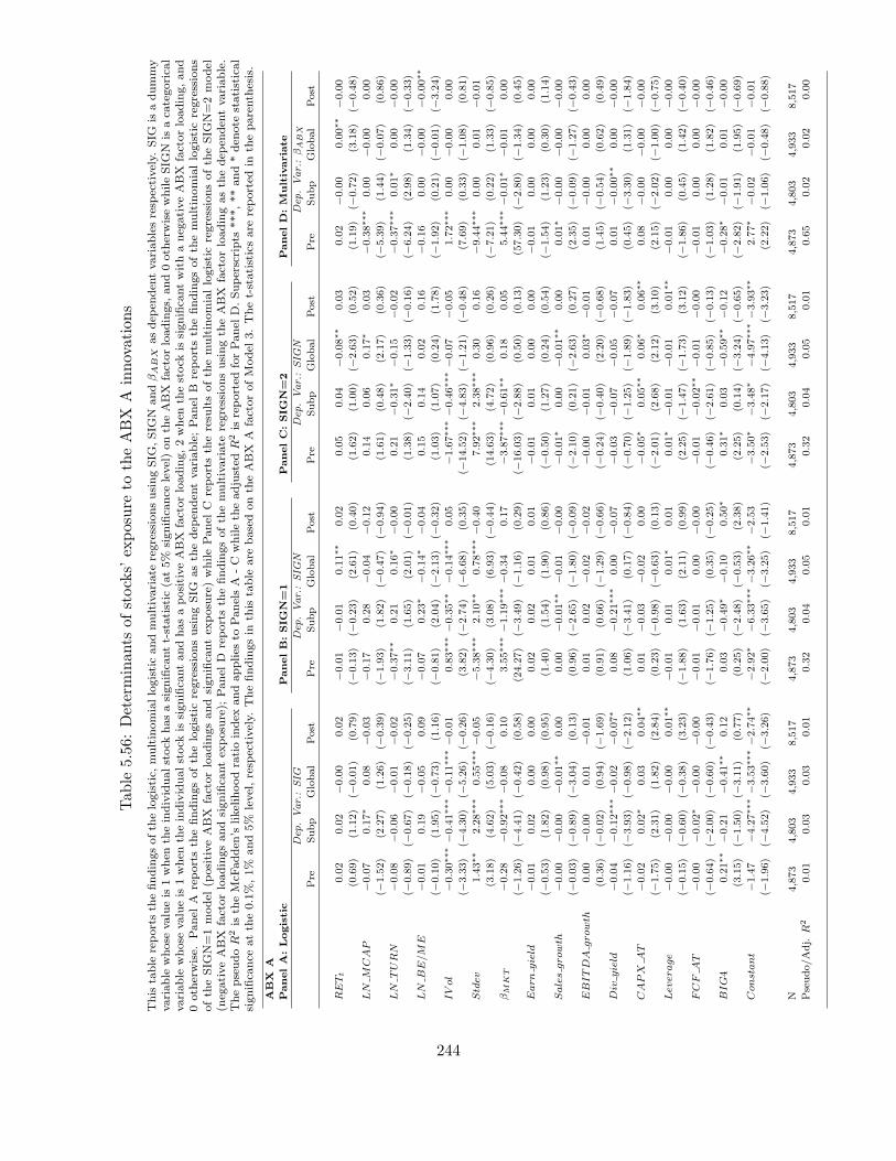
Tab
le5.56:Determinants
ofstocks’
exposure
totheABX
Ainnovations
This
table
reportsth
efindingsofth
elogistic,
multinomiallogisticandmultivariate
regressionsusingSIG
,SIG
NandβABX
asdep
enden
tvariablesresp
ectively.
SIG
isadummy
variable
whose
valueis
1when
theindividualstock
hasasignifica
ntt-statistic
(at5%
significa
nce
level)onth
eABX
factorloadings,
and0oth
erwisewhileSIG
Nis
aca
tegorica
lvariable
whose
valueis
1when
theindividualstock
issignifica
ntandhasapositiveABX
factorloading,2when
thestock
issignifica
ntwithaneg
ativeABX
factorloading,and
0oth
erwise.
Panel
Areportsth
efindingsofth
elogisticregressionsusingSIG
asth
edep
enden
tvariable;Panel
Breportsth
efindingsofth
emultinomiallogisticregressions
ofth
eSIG
N=1model
(positiveABX
factorloadingsandsignifica
ntex
posu
re)whilePanel
Creportsth
eresu
ltsofth
emultinomiallogisticregressionsofth
eSIG
N=2model
(neg
ativeABX
factorloadingsandsignifica
ntex
posu
re);
Panel
Dreportsth
efindingsofth
emultivariate
regressionsusingth
eABX
factorloadingasth
edep
enden
tvariable.
ThepseudoR
2is
theMcF
adden
’slikelihoodratioindex
andapplies
toPanelsA
-C
whileth
eadjusted
R2is
reported
forPanel
D.Superscripts
***,**and*den
ote
statistical
significa
nce
atth
e0.1%,1%
and5%
level,resp
ectively.
Thefindingsin
this
table
are
basedonth
eABX
AfactorofModel
3.Thet-statisticsare
reported
inth
eparenth
esis.
ABX
A
PanelA:Logistic
PanelB:SIG
N=1
PanelC:SIG
N=2
PanelD:M
ultivariate
Dep
.Var.:SIG
Dep
.Var.:SIG
NDep
.Var.:SIG
NDep
.Var.:βABX
Pre
Subp
Global
Post
Pre
Subp
Global
Post
Pre
Subp
Global
Post
Pre
Subp
Global
Post
RETt
0.02
0.02
−0.00
0.02
−0.01
−0.01
0.11∗∗
0.02
0.05
0.04
−0.08∗∗
0.03
0.02
−0.00
0.00∗∗
−0.00
(0.69)
(1.12)
(−0.01)
(0.79)
(−0.13)
(−0.23)
(2.61)
(0.40)
(1.62)
(1.00)
(−2.63)
(0.52)
(1.19)
(−0.72)
(3.18)
(−0.48)
LN
MCAP
−0.07
0.17∗
0.08
−0.03
−0.17
0.28
−0.04
−0.12
0.14
0.06
0.17∗
0.03
−0.38∗∗
∗0.00
−0.00
0.00
(−1.52)
(2.27)
(1.26)
(−0.39)
(−1.93)
(1.82)
(−0.47)
(−0.94)
(1.61)
(0.48)
(2.17)
(0.36)
(−5.39)
(1.44)
(−0.07)
(0.86)
LN
TURN
−0.08
−0.06
−0.01
−0.02
−0.37∗∗
0.21
0.16∗
−0.00
0.21
−0.31∗
−0.15
−0.02
−0.37∗∗
∗0.01∗
0.00
−0.00
(−0.89)
(−0.67)
(−0.18)
(−0.25)
(−3.11)
(1.65)
(2.01)
(−0.01)
(1.38)
(−2.40)
(−1.33)
(−0.16)
(−6.24)
(2.98)
(1.34)
(−0.33)
LN
BE/M
E−0.01
0.19
−0.05
0.09
−0.07
0.23∗
−0.14∗
−0.04
0.15
0.14
0.02
0.16
−0.16
0.00
−0.00
−0.00∗∗
(−0.10)
(1.95)
(−0.73)
(1.16)
(−0.81)
(2.04)
(−2.13)
(−0.32)
(1.03)
(1.07)
(0.24)
(1.78)
(−1.92)
(0.21)
(−0.01)
(−3.24)
IVol
−0.30∗∗
∗−0.41∗∗
∗−0.11∗∗
∗−0.01
0.83∗∗
∗−0.35∗∗
−0.14∗∗
∗0.05
−1.67∗∗
∗−0.46∗∗
∗−0.07
−0.05
1.72∗∗
∗0.00
−0.00
0.00
(−3.33)
(−4.30)
(−5.26)
(−0.26)
(3.82)
(−2.74)
(−6.68)
(0.35)
(−14.52)
(−4.83)
(−1.21)
(−0.48)
(7.69)
(0.33)
(−1.08)
(0.81)
Stdev
1.43∗∗
2.28∗∗
∗0.55∗∗
∗−0.05
−5.38∗∗
∗2.10∗∗
0.78∗∗
∗−0.40
7.92∗∗
∗2.38∗∗
∗0.30
0.16
−9.44∗∗
∗0.00
0.01
−0.01
(3.18)
(4.62)
(5.03)
(−0.16)
(−4.30)
(3.08)
(6.93)
(−0.44)
(14.63)
(4.72)
(0.96)
(0.26)
(−7.21)
(0.22)
(1.33)
(−0.85)
βM
KT
−0.28
−0.92∗∗
∗−0.08
0.10
3.55∗∗
∗−1.19∗∗
∗−0.34
0.17
−3.87∗∗
∗−0.61∗∗
0.18
0.05
5.44∗∗
∗−0.01∗
−0.01
0.00
(−1.26)
(−4.41)
(−0.42)
(0.58)
(24.27)
(−3.49)
(−1.16)
(0.29)
(−16.03)
(−2.88)
(0.50)
(0.13)
(57.30)
(−2.80)
(−1.34)
(0.45)
Earn
yield
−0.01
0.02
0.00
0.00
0.02
0.02
0.01
0.01
−0.01
0.01
0.00
0.00
−0.01
0.00
0.00
0.00
(−0.53)
(1.82)
(0.98)
(0.95)
(1.40)
(1.54)
(1.90)
(0.86)
(−0.50)
(1.27)
(0.24)
(0.54)
(−1.54)
(1.23)
(0.30)
(1.14)
Salesgrowth
−0.00
−0.00
−0.01∗∗
0.00
0.00
−0.01∗∗
−0.01
−0.00
−0.01∗
0.00
−0.01∗∗
0.00
0.01∗
−0.00
−0.00
−0.00
(−0.03)
(−0.89)
(−3.04)
(0.13)
(0.96)
(−2.65)
(−1.80)
(−0.09)
(−2.10)
(0.21)
(−2.63)
(0.27)
(2.35)
(−0.09)
(−1.27)
(−0.43)
EBITDA
growth
0.00
−0.00
0.01
−0.01
0.01
0.02
−0.02
−0.02
−0.00
−0.01
0.03∗
−0.01
0.01
−0.00
0.00
0.00
(0.36)
(−0.02)
(0.94)
(−1.69)
(0.91)
(0.66)
(−1.29)
(−0.66)
(−0.24)
(−0.40)
(2.20)
(−0.68)
(1.45)
(−0.54)
(0.62)
(0.49)
Div
yield
−0.04
−0.12∗∗
∗−0.02
−0.07∗
0.08
−0.21∗∗
∗0.00
−0.07
−0.03
−0.07
−0.05
−0.07
0.01
−0.00∗∗
0.00
−0.00
(−1.16)
(−3.93)
(−0.98)
(−2.12)
(1.06)
(−3.41)
(0.17)
(−0.84)
(−0.70)
(−1.25)
(−1.89)
(−1.83)
(0.45)
(−3.30)
(1.31)
(−1.84)
CAPX
AT
−0.02
0.02∗
0.03
0.04∗∗
0.01
−0.03
−0.02
0.00
−0.05∗
0.05∗∗
0.06∗
0.06∗∗
0.08
−0.00
−0.00
−0.00
(−1.75)
(2.31)
(1.82)
(2.84)
(0.23)
(−0.98)
(−0.63)
(0.13)
(−2.01)
(2.68)
(2.12)
(3.10)
(2.15)
(−2.02)
(−1.00)
(−0.75)
Lev
erage
−0.00
−0.00
−0.00
0.01∗∗
−0.01
0.01
0.01∗
0.01
0.01∗
−0.01
−0.01
0.01∗∗
−0.01
0.00
0.00
−0.00
(−0.15)
(−0.60)
(−0.38)
(3.23)
(−1.88)
(1.63)
(2.11)
(0.99)
(2.25)
(−1.47)
(−1.73)
(3.12)
(−1.86)
(0.45)
(1.42)
(−0.40)
FCF
AT
−0.00
−0.02∗
−0.00
−0.00
−0.01
−0.01
0.00
−0.00
−0.01
−0.02∗∗
−0.01
−0.00
−0.01
0.00
0.00
−0.00
(−0.64)
(−2.00)
(−0.60)
(−0.43)
(−1.76)
(−1.25)
(0.35)
(−0.25)
(−0.46)
(−2.61)
(−0.85)
(−0.13)
(−1.03)
(1.28)
(1.82)
(−0.46)
BIG4
0.21∗∗
−0.21
−0.41∗∗
0.12
0.03
−0.49∗
−0.10
0.50∗
0.31∗
0.03
−0.59∗∗
−0.12
−0.28∗
−0.01
0.01
−0.00
(3.15)
(−1.50)
(−3.11)
(0.77)
(0.25)
(−2.48)
(−0.53)
(2.38)
(2.25)
(0.14)
(−3.24)
(−0.65)
(−2.82)
(−1.91)
(1.95)
(−0.69)
Constant
−1.47
−4.27∗∗
∗−3.53∗∗
∗−2.74∗∗
−2.92∗
−6.33∗∗
∗−3.26∗∗
−2.53
−3.50∗
−3.48∗
−4.97∗∗
∗−3.93∗∗
2.77∗
−0.02
−0.01
−0.01
(−1.96)
(−4.52)
(−3.60)
(−3.26)
(−2.00)
(−3.65)
(−3.25)
(−1.41)
(−2.53)
(−2.17)
(−4.13)
(−3.23)
(2.22)
(−1.06)
(−0.48)
(−0.88)
N4,873
4,803
4,933
8,517
4,873
4,803
4,933
8,517
4,873
4,803
4,933
8,517
4,873
4,803
4,933
8,517
Pseudo/Adj.
R2
0.01
0.03
0.03
0.01
0.32
0.04
0.05
0.01
0.32
0.04
0.05
0.01
0.65
0.02
0.02
0.00
244
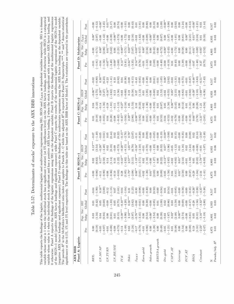
Tab
le5.57
:Determinants
ofstocks’
exposure
totheABX
BBB
innovations
This
table
reportsth
efindingsofth
elogistic,
multinomiallogisticandmultivariate
regressionsusingSIG
,SIG
NandβABX
asdep
enden
tvariablesresp
ectively.
SIG
isadummy
variable
whose
valueis
1when
theindividualstock
hasasignifica
ntt-statisti(at5%
significa
nce
level)onth
eABX
factorloadings,
and0oth
erwisewhileSIG
Nis
aca
tegorica
lvariable
whose
valueis
1when
theindividualstock
issignifica
ntandhasapositiveABX
factorloading,2when
thestock
issignifica
ntwithaneg
ativeABX
factorloading,and
0oth
erwise.
Panel
Areportsth
efindingsofth
elogisticregressionsusingSIG
asth
edep
enden
tvariable;Panel
Breportsth
efindingsofth
emultinomiallogisticregressions
ofth
eSIG
N=1model
(positiveABX
factorloadingsandsignifica
ntex
posu
re)whilePanel
Creportsth
eresu
ltsofth
emultinomiallogisticregressionsofth
eSIG
N=2model
(neg
ativeABX
factorloadingsandsignifica
ntex
posu
re);
Panel
Dreportsth
efindingsofth
emultivariate
regressionsusingth
eABX
factorloadingasth
edep
enden
tvariable.
ThepseudoR
2is
theMcF
adden
’slikelihoodratioindex
andapplies
toPanelsA
-C
whileth
eadjusted
R2is
reported
forPanel
D.Superscripts
***,**and*den
ote
statistical
significa
nce
atth
e0.1%,1%
and5%
level
resp
ectively.
Thefindingsin
this
table
are
basedonth
eABX
BBB
factorofModel
3.Thet-statisticsare
reported
inth
eparenth
esis.
ABX
BBB
PanelA:Logistic
PanelB:SIG
N=1
PanelC:SIG
N=2
PanelD:M
ultivariate
Dep
.Var.:SIG
Dep
.Var.:SIG
NDep
.Var.:SIG
NDep
.Var.:βABX
Pre
Subp
Global
Post
Pre
Subp
Global
Post
Pre
Subp
Global
Post
Pre
Subp
Global
Post
RETt
0.00
0.03
0.01
−0.04
−0.00
0.02
0.13∗∗
∗−0.07
0.01
0.04
−0.06∗∗
−0.02
−0.01
−0.00
0.00∗
−0.00
(0.19)
(1.34)
(0.42)
(−1.90)
(−0.06)
(0.63)
(3.54)
(−1.40)
(0.19)
(1.43)
(−2.75)
(−0.80)
(−1.81)
(−0.71)
(2.97)
(−0.12)
LN
MCAP
−0.05
0.04
0.05
0.16∗∗
−0.11
0.17∗∗
−0.20∗
−0.05
−0.00
−0.14
0.20∗∗
0.30∗∗
∗−0.04
0.00∗
−0.00
−0.00∗
(−0.87)
(0.94)
(0.69)
(3.00)
(−0.90)
(2.58)
(−2.48)
(−0.61)
(−0.05)
(−1.56)
(3.27)
(6.23)
(−1.56)
(2.86)
(−1.42)
(−2.45)
LN
TURN
−0.01
0.00
−0.09
−0.12
−0.06
0.14
0.02
0.05
0.04
−0.19
−0.16∗∗
−0.23
−0.07∗∗
0.01∗∗
∗−0.00
0.01∗∗
∗
(−0.08)
(0.01)
(−1.33)
(−1.15)
(−0.36)
(1.14)
(0.18)
(0.44)
(0.28)
(−1.81)
(−2.62)
(−1.41)
(−3.48)
(5.62)
(−0.39)
(5.17)
LN
BE/M
E−0.09
0.01
0.05
0.07
−0.10
0.10
−0.09
0.02
−0.08
−0.11
0.13
0.10
−0.09∗
0.00
−0.00∗∗
0.00
(−0.73)
(0.15)
(0.75)
(1.61)
(−0.83)
(1.22)
(−0.73)
(0.22)
(−0.42)
(−1.13)
(1.56)
(0.92)
(−2.60)
(1.21)
(−3.73)
(0.74)
IVol
−0.14
−0.38∗∗
∗−0.10∗∗
∗−0.04
0.28
−0.43∗∗
−0.20∗∗
∗−0.15∗∗
−0.45∗∗
−0.27∗
−0.03
0.04
0.14∗∗
−0.00∗∗
−0.00
−0.00
(−1.49)
(−3.90)
(−4.20)
(−1.04)
(1.85)
(−2.82)
(−8.15)
(−2.76)
(−3.04)
(−2.16)
(−0.60)
(0.36)
(3.41)
(−3.71)
(−1.72)
(−1.01)
Stdev
0.63
2.10∗∗
∗0.56∗∗
∗0.31
−1.79∗
2.57∗∗
1.05∗∗
∗0.78∗
2.29∗∗
1.05
0.19
−0.09
−0.84∗∗
0.03∗∗
∗0.02
0.00
(1.24)
(3.97)
(3.62)
(1.25)
(−2.08)
(3.15)
(6.70)
(2.07)
(2.80)
(1.53)
(0.58)
(−0.15)
(−3.35)
(5.07)
(2.16)
(0.43)
βM
KT
−0.17
−0.76∗∗
∗−0.00
−0.30
0.86∗∗
−1.19∗∗
∗−0.58∗
−0.11
−0.98∗∗
∗0.10
0.37
−0.43
0.54∗∗
∗−0.03∗∗
∗−0.02
0.01
(−0.79)
(−3.45)
(−0.01)
(−0.98)
(3.01)
(−3.71)
(−2.10)
(−0.20)
(−3.82)
(0.33)
(1.13)
(−0.95)
(9.76)
(−9.57)
(−1.63)
(1.91)
Earn
yield
−0.01
0.00
0.00
−0.00
−0.02
0.02
−0.01
0.00
0.00
−0.02
0.01
−0.00
−0.01
0.00∗
−0.00
0.00
(−0.86)
(0.54)
(0.39)
(−0.30)
(−1.26)
(1.16)
(−0.78)
(0.09)
(0.01)
(−1.36)
(1.05)
(−0.48)
(−1.22)
(2.34)
(−0.09)
(0.80)
Salesgrowth
0.00
−0.00∗
−0.00
0.00
0.01∗
−0.00
−0.00
−0.00
−0.00
−0.00
−0.00
0.00
0.00
0.00
−0.00∗
0.00
(1.28)
(−2.54)
(−0.95)
(0.50)
(2.03)
(−1.27)
(−1.23)
(−0.05)
(−1.24)
(−0.93)
(−0.68)
(0.61)
(1.69)
(0.42)
(−2.92)
(0.18)
EBITDA
growth
0.00
0.00
0.01
−0.00
0.00
0.00
0.00
−0.00
0.01
0.01
0.02
−0.01
−0.00
−0.00
0.00
0.00
(0.49)
(0.39)
(1.00)
(−0.94)
(0.09)
(0.22)
(0.32)
(−0.19)
(0.53)
(0.67)
(1.53)
(−1.05)
(−0.40)
(−0.72)
(0.67)
(1.09)
Div
yield
−0.05
−0.03
0.02
0.01
−0.05
−0.13∗∗
0.07∗
−0.09∗∗
−0.04
0.05
−0.02
0.06∗
−0.00
−0.00∗
0.00
−0.00∗∗
(−1.21)
(−1.67)
(0.86)
(0.54)
(−1.56)
(−2.65)
(1.96)
(−3.00)
(−0.53)
(1.50)
(−0.55)
(2.02)
(−0.19)
(−2.43)
(1.07)
(−3.08)
CAPX
AT
0.01
0.02∗
0.03
−0.01
0.04
−0.02
−0.05
0.00
−0.02
0.06∗∗
∗0.05∗
−0.03
0.01
−0.00
−0.00
0.00
(0.48)
(2.48)
(1.59)
(−0.85)
(1.61)
(−0.92)
(−1.12)
(0.15)
(−0.79)
(3.45)
(2.15)
(−1.31)
(0.43)
(−1.72)
(−1.01)
(2.02)
Lev
erage
0.00
0.00∗∗
0.00
−0.00
0.01∗
0.01∗
0.01
−0.00
−0.00
0.00
−0.00
−0.00
0.00
0.00
0.00
0.00
(1.54)
(2.74)
(0.69)
(−0.56)
(2.50)
(2.44)
(1.16)
(−0.35)
(−0.04)
(0.12)
(−0.82)
(−0.75)
(1.39)
(0.58)
(0.81)
(1.24)
FCF
AT
0.00
−0.00
−0.00
−0.00
0.00
−0.01
0.02
0.00
−0.00
0.01
−0.01
−0.01
−0.00
0.00
0.00∗
−0.00
(0.09)
(−0.81)
(−0.17)
(−0.35)
(0.37)
(−1.59)
(1.24)
(0.09)
(−0.18)
(1.31)
(−0.92)
(−0.87)
(−1.66)
(0.11)
(2.21)
(−0.13)
BIG4
0.19
0.05
−0.28
−0.26∗
−0.29
0.05
−0.00
0.02
0.66∗∗
∗0.06
−0.39∗
−0.48∗∗
∗−0.07
−0.01∗
0.01∗∗
−0.00∗
(1.31)
(0.31)
(−1.56)
(−2.26)
(−1.84)
(0.22)
(−0.00)
(0.14)
(3.78)
(0.28)
(−2.10)
(−3.83)
(−1.48)
(−3.09)
(3.24)
(−2.21)
Constant
−2.23∗
−3.16∗∗
∗−3.32∗∗
−4.35∗∗
∗−2.44
−5.78∗∗
∗−0.91
−2.94∗
−3.21∗∗
−1.21
−5.69∗∗
∗−6.51∗∗
∗0.27
−0.05∗
0.01
0.03
(−2.47)
(−5.19)
(−2.80)
(−5.48)
(−1.41)
(−6.93)
(−1.07)
(−2.48)
(−2.65)
(−0.94)
(−6.36)
(−7.43)
(0.75)
(−2.52)
(0.33)
(1.44)
N4,873
4,803
4,933
8,517
4,873
4,803
4,933
8,517
4,873
4,803
4,933
8,517
4,873
4,803
4,933
8,517
Pseudo/Adj.
R2
0.01
0.02
0.03
0.01
0.03
0.03
0.06
0.02
0.03
0.03
0.06
0.02
0.03
0.03
0.03
0.02
245
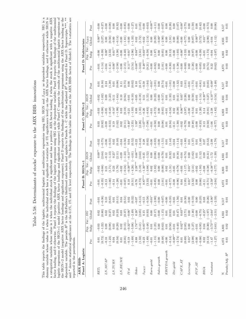
Tab
le5.58
:Determinants
ofstocks’
exposure
totheABX
BBB-innovations
This
table
reportsth
efindingsofth
elogistic,
multinomiallogisticand
multivariate
regressionsusingSIG
,SIG
Nand
βABX
asdep
enden
tvariablesresp
ectively.
SIG
isa
dummyvariable
whose
valueis
1when
theindividualstock
hasasignifica
ntt-statistic
(at5%
significa
nce
level)onth
eABX
factorloadings,
and0oth
erwisewhileSIG
Nis
aca
tegorica
lvariable
whose
valueis
1when
theindividualstock
issignifica
ntand
hasapositiveABX
factorloading,2when
thestock
issignifica
ntwith
aneg
ativeABX
factorloading,and0oth
erwise.
Panel
Areportsth
efindingsofth
elogisticregressionsusingSIG
asth
edep
enden
tvariable;Panel
Breportsth
efindingsofth
emultinomial
logisticregressionsofth
eSIG
N=1model
(positiveABX
factorloadingsandsignifica
ntex
posu
re)whilePanel
Creportsth
eresu
ltsofth
emultinomiallogisticregressionsof
theSIG
N=2model
(neg
ativeABX
factorloadingsandsignifica
ntex
posu
re);
Panel
Dreportsth
efindingsofth
emultivariate
regressionsusingth
eABX
factorloadingasth
edep
enden
tvariable.ThepseudoR
2is
theMcF
adden
’slikelihoodratioindex
andapplies
toPanelsA
-C
whileth
eadjusted
R2is
reported
forPanel
D.Superscripts
***,**
and*den
ote
statisticalsignifica
nce
atth
e0.1%,1%
and5%
level
resp
ectively.
Thefindingsin
this
table
are
basedonth
eABX
BBB-factorofModel
3.Thet-statisticsare
reported
inth
eparenth
esis.
ABX
BBB-
PanelA:Logistic
PanelB:SIG
N=1
PanelC:SIG
N=2
PanelD:M
ultivariate
Dep
.Var.:SIG
Dep
.Var.:SIG
NDep
.Var.:SIG
NDep
.Var.:βABX
Pre
Subp
Global
Post
Pre
Subp
Global
Post
Pre
Subp
Global
Post
Pre
Subp
Global
Post
RETt
0.01
−0.03
0.02
−0.01
−0.01
−0.02
0.09∗∗
−0.02
0.03
−0.03
−0.02
0.01
−0.01
−0.00
0.00∗∗
−0.00
(0.72)
(−1.22)
(0.80)
(−0.36)
(−0.35)
(−0.66)
(2.64)
(−0.75)
(0.92)
(−0.98)
(−1.02)
(0.16)
(−1.14)
(−0.39)
(3.27)
(−0.27)
LN
MCAP
−0.10
0.09
0.02
0.10
−0.13
0.21
−0.12
−0.06
−0.09
−0.05
0.09
0.24
−0.04
0.00∗
0.00
−0.00
(−1.23)
(0.98)
(0.27)
(0.85)
(−1.66)
(1.71)
(−1.13)
(−0.55)
(−0.53)
(−0.48)
(1.23)
(1.38)
(−1.41)
(2.33)
(0.56)
(−0.08)
LN
TURN
0.04
0.03
0.02
0.01
−0.14
0.23
0.25∗
0.02
0.19
−0.16∗
−0.11
0.01
−0.06∗
0.01∗∗
−0.00
0.00
(0.34)
(0.29)
(0.23)
(0.11)
(−1.28)
(1.76)
(2.11)
(0.10)
(1.02)
(−1.99)
(−1.64)
(0.08)
(−2.58)
(3.38)
(−0.14)
(0.32)
LN
BE/M
E0.01
0.02
0.03
0.04
−0.01
−0.02
−0.09
−0.04
0.02
0.03
0.10
0.11
−0.06
−0.00
−0.00
−0.00
(0.05)
(0.15)
(0.37)
(0.51)
(−0.07)
(−0.24)
(−1.23)
(−0.56)
(0.11)
(0.18)
(0.94)
(0.75)
(−2.15)
(−0.40)
(−1.81)
(−0.85)
IVol
−0.19
−0.32∗∗
∗−0.06∗
0.02
0.10
−0.39∗∗
∗−0.14∗∗
∗0.04
−0.40∗
−0.21
−0.01
0.00
0.11∗∗
−0.01∗
−0.00
−0.00
(−1.69)
(−5.08)
(−2.49)
(0.32)
(0.51)
(−4.26)
(−4.01)
(0.52)
(−2.35)
(−1.93)
(−0.10)
(0.02)
(3.54)
(−2.96)
(−1.33)
(−1.27)
Stdev
0.88
1.74∗∗
∗0.26∗
−0.07
−0.76
2.28∗∗
∗0.66∗∗
∗−0.22
1.99∗
0.89
−0.05
0.10
−0.68∗∗
0.04∗∗
0.02
0.01
(1.59)
(5.41)
(2.05)
(−0.15)
(−0.73)
(5.19)
(3.63)
(−0.44)
(2.26)
(1.35)
(−0.18)
(0.17)
(−3.63)
(3.31)
(1.72)
(1.05)
βM
KT
−0.23
−0.85∗∗
∗0.15
−0.15
0.87∗∗
∗−1.30∗∗
∗−0.35
0.28
−1.07∗∗
∗−0.26
0.51
−0.58
0.48∗∗
∗−0.03∗∗
∗−0.02
−0.00
(−1.89)
(−3.48)
(0.93)
(−0.58)
(3.33)
(−3.88)
(−1.52)
(0.92)
(−7.08)
(−0.83)
(1.55)
(−1.64)
(9.21)
(−6.59)
(−2.14)
(−0.63)
Earn
yield
−0.01
0.01
0.00
−0.01∗
−0.01
0.02
0.00
−0.00
−0.01
−0.01
0.00
−0.01∗
−0.00
0.00
0.00
−0.00∗∗
(−1.15)
(1.25)
(0.17)
(−2.00)
(−0.85)
(1.82)
(0.06)
(−0.93)
(−0.50)
(−0.72)
(0.23)
(−2.01)
(−0.82)
(1.87)
(0.29)
(−4.11)
Salesgrowth
0.00
0.00
−0.00
−0.00
0.00
0.00
−0.00
−0.00
0.00
0.00
−0.00
0.00
0.00
0.00
−0.00∗
−0.00
(0.48)
(0.63)
(−1.15)
(−0.07)
(1.01)
(0.00)
(−0.70)
(−1.51)
(0.08)
(0.65)
(−0.57)
(0.74)
(1.01)
(0.05)
(−2.90)
(−0.07)
EBITDA
growth
−0.00
0.01
0.01
−0.00
−0.01
0.02
0.01
0.01
0.01
−0.01
0.01
−0.01
−0.00
0.00
0.00
0.00
(−0.14)
(0.56)
(0.93)
(−0.35)
(−0.77)
(1.31)
(0.32)
(1.44)
(0.34)
(−0.34)
(1.33)
(−1.01)
(−0.30)
(0.13)
(1.91)
(0.26)
Div
yield
−0.09∗∗
−0.01
0.01
−0.05
−0.08
−0.05
0.01
−0.04
−0.11
0.02
0.01
−0.08
−0.01
−0.00
0.00
0.00
(−2.74)
(−0.40)
(0.47)
(−1.56)
(−0.96)
(−0.78)
(0.16)
(−1.14)
(−1.30)
(0.39)
(0.41)
(−1.32)
(−1.38)
(−1.03)
(0.00)
(1.07)
CAPX
AT
0.01
0.02∗∗
0.03∗∗
0.01
0.04
−0.03
−0.04
−0.03
−0.02
0.06∗∗
∗0.05∗
0.03
−0.00
−0.00∗
−0.00
−0.00∗
(0.69)
(2.85)
(2.71)
(0.30)
(1.95)
(−1.17)
(−0.74)
(−1.80)
(−0.79)
(3.97)
(2.26)
(1.61)
(−0.00)
(−2.33)
(−0.77)
(−2.75)
Lev
erage
0.01∗
0.00
0.00
−0.00
0.01∗
0.01∗
0.00
0.01
0.00
−0.00
0.00
−0.01
0.00
0.00
0.00
0.00
(2.09)
(1.27)
(1.46)
(−0.10)
(2.32)
(2.41)
(1.62)
(1.37)
(0.48)
(−0.54)
(0.50)
(−1.75)
(1.26)
(0.97)
(0.87)
(1.50)
FCF
AT
−0.00
−0.01
−0.00
0.00
0.00
−0.02
0.01
0.01
−0.00
0.01
−0.01
−0.01
−0.00
−0.00
0.00∗∗
0.00
(−0.08)
(−0.95)
(−0.75)
(0.25)
(0.66)
(−1.93)
(1.12)
(1.48)
(−0.23)
(1.20)
(−1.14)
(−0.81)
(−0.05)
(−0.39)
(3.72)
(0.42)
BIG4
0.02
0.04
−0.25∗
0.03
−0.11
−0.08
0.09
0.07
0.13
0.14
−0.39∗∗
0.01
0.03
−0.01
0.01∗
−0.00
(0.13)
(0.30)
(−1.97)
(0.26)
(−0.71)
(−0.38)
(0.31)
(0.53)
(0.50)
(0.91)
(−3.27)
(0.05)
(0.74)
(−1.73)
(2.90)
(−0.73)
Constant
−1.47
−3.73∗∗
∗−2.64∗
−3.90∗
−2.59∗
−6.38∗∗
∗−1.72
−2.99
−1.66
−2.38
−4.10∗∗
∗−6.09∗
0.22
−0.04
−0.04
0.00
(−1.27)
(−3.61)
(−2.51)
(−2.33)
(−2.04)
(−3.77)
(−1.39)
(−1.78)
(−0.77)
(−1.82)
(−3.54)
(−2.48)
(0.62)
(−2.07)
(−1.12)
(0.06)
N4,873
4,803
4,933
8,517
4,873
4,803
4,933
8,517
4,873
4,803
4,933
8,517
4,873
4,803
4,933
8,517
Pseudo/Adj.
R2
0.01
0.02
0.02
0.01
0.03
0.03
0.04
0.02
0.03
0.03
0.04
0.02
0.03
0.02
0.03
0.01
246
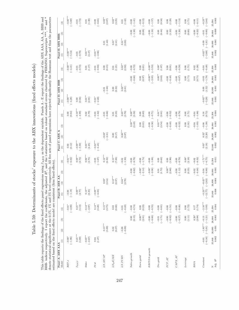
Tab
le5.59
:Determinants
ofstocks’
exposure
totheABX
innovations(fixed
effects
models)
This
table
reportsth
efindingsofth
efixed
effects
panel
regressionsusingβABX
asth
edep
enden
tvariable.PanelsA
-E
report
thefindingsofth
eABX
AAA,AA,A,BBB
and
BBB-indices
resp
ectively.
Ireport
theco
efficien
ts,th
eadjusted
R2,andth
et-statisticsbasedonrobust
standard
errors
clustered
byPERMNO.Superscripts
***,**and*
den
ote
statisticalsignifica
nce
atth
e0.1%,1%
and5%
level
resp
ectively.
Allfivesets
ofpanel
regressionshaverejected
significa
ntlyth
eHausm
antest
andthusth
eparameters
estimatedbasedonth
efixed
effects
model
are
consisten
t(fi
rmfixed
effects).
PanelA:ABX
AAA
PanelB:ABX
AA
PanelC:ABX
APanelD:ABX
BBB
PanelE:ABX
BBB-
Model
(1)
(2)
(3)
(4)
(1)
(2)
(3)
(4)
(1)
(2)
(3)
(4)
(1)
(2)
(3)
(4)
(1)
(2)
(3)
(4)
RET
t−0.00∗
−0.01∗
−0.00
−0.01∗∗
∗0.00
0.00
−0.00∗∗
∗−0.00∗∗
∗−0.00∗∗
∗−0.00∗∗
∗
(−1.96)
(−2.00)
(−1.19)
(−6.02)
(0.12)
(0.04)
(−4.26)
(−4.41)
(−5.54)
(−5.60)
βM
KT
0.21∗∗
∗0.21∗∗
∗0.09∗∗
∗0.08∗∗
∗−0.09∗∗
∗−0.10∗∗
∗0.00
−0.01
−0.01
−0.01
(4.89)
(4.13)
(4.77)
(3.73)
(−5.50)
(−4.99)
(0.56)
(−0.72)
(−0.79)
(−1.73)
Stdev
−0.07∗∗
−0.14∗∗
∗0.10∗∗
∗0.06∗∗
∗0.05∗∗
∗0.02
0.01∗∗
0.01
0.01∗∗
∗0.01
(−2.67)
(−3.97)
(8.35)
(3.75)
(4.25)
(1.79)
(2.91)
(1.17)
(3.47)
(1.30)
IVol
0.04
0.14∗∗
−0.09∗∗
∗−0.03
−0.04∗∗
∗−0.03
−0.01∗
−0.01
−0.01∗∗
−0.00
(1.27)
(3.20)
(−6.05)
(−1.67)
(−3.45)
(−1.62)
(−2.20)
(−0.93)
(−2.98)
(−0.65)
LN
MCAP
0.15∗∗
∗0.15∗∗
∗0.03∗
0.12∗∗
∗−0.03∗
−0.01
−0.01
0.00
0.01
0.02∗∗
(5.09)
(3.75)
(2.54)
(6.32)
(−2.31)
(−0.66)
(−1.68)
(0.15)
(1.43)
(2.87)
LN
BE/M
E0.02
0.03
0.12∗∗
∗0.15∗∗
∗0.00
0.01
0.00
0.01
0.01∗
0.02∗∗
(0.57)
(0.80)
(8.37)
(7.88)
(0.17)
(0.35)
(0.22)
(1.21)
(2.41)
(3.25)
LN
TURN
−0.00
−0.01
0.04∗∗
−0.02
0.06∗∗
∗0.05∗∗
∗0.02∗∗
∗0.02∗∗
0.01∗∗
0.01
(−0.09)
(−0.22)
(2.70)
(−1.50)
(5.07)
(3.70)
(3.81)
(2.92)
(3.03)
(1.42)
Salesgrowth
0.00
−0.00
−0.00
−0.00
0.00∗∗
∗0.00∗∗
∗−0.00
−0.00
−0.00
−0.00
(0.15)
(−0.74)
(−0.82)
(−0.79)
(3.49)
(3.50)
(−0.66)
(−0.72)
(−1.38)
(−1.41)
Earn
yield
0.00∗∗
0.00
−0.00∗
−0.00
0.00
0.00
0.00
0.00
0.00
−0.00
(2.81)
(0.23)
(−2.14)
(−1.74)
(0.01)
(0.83)
(0.97)
(0.81)
(0.08)
(−0.12)
EBITDA
growth
−0.00
−0.00
−0.00∗
−0.00
−0.00
−0.00
−0.00∗∗
−0.00∗∗
∗−0.00
−0.00
(−0.66)
(−0.55)
(−2.06)
(−1.88)
(−0.38)
(−0.71)
(−2.85)
(−3.53)
(−1.24)
(−1.57)
Div
yield
−0.01
−0.00
0.01
0.00
0.01∗∗
∗0.01∗∗
0.00∗∗
0.00∗
0.00
0.00
(−1.71)
(−0.01)
(1.72)
(0.62)
(3.54)
(2.61)
(2.63)
(1.97)
(0.44)
(0.34)
FCF
AT
−0.00
−0.00
0.00∗∗
0.00
−0.00
−0.00
−0.00
0.00
0.00
0.00
(−0.92)
(−1.51)
(2.80)
(1.96)
(−0.40)
(−0.52)
(−0.48)
(0.01)
(1.33)
(1.29)
CAPX
AT
−0.00
−0.00
−0.00
−0.00
−0.00
−0.00
−0.00
−0.00
−0.00
−0.00
(−0.57)
(−0.46)
(−1.12)
(−0.70)
(−0.32)
(−0.78)
(−0.87)
(−0.59)
(−1.26)
(−1.14)
Lev
erage
0.00
0.00
0.00
0.00∗
0.00
0.00
0.00
0.00
0.00
0.00
(1.11)
(1.72)
(0.35)
(2.10)
(1.91)
(1.71)
(1.71)
(1.71)
(0.60)
(1.71)
BIG4
0.20∗
0.17
−0.02
−0.02
−0.04
−0.04
0.01
0.02
−0.00
−0.00
(2.08)
(1.74)
(−0.48)
(−0.32)
(−1.03)
(−1.00)
(0.71)
(1.20)
(−0.22)
(−0.11)
Constant
−0.01
−1.83∗∗
∗−0.13
−2.18∗∗
∗−0.23∗∗
∗−0.45∗∗
−0.04
−1.71∗∗
∗0.03∗
0.32∗
−0.06
0.16
−0.02∗∗
0.09
−0.03
−0.04
−0.02∗∗
−0.09
−0.01
−0.23∗∗
(−0.16)
(−5.01)
(−1.21)
(−3.93)
(−12.77)
(−2.63)
(−0.80)
(−6.75)
(2.16)
(2.20)
(−1.39)
(0.72)
(−3.20)
(1.52)
(−1.78)
(−0.48)
(−2.69)
(−1.61)
(−0.60)
(−2.84)
N35,846
26,890
26,884
25,304
35,846
26,890
26,884
25,304
35,846
26,890
26,884
25,304
35,846
26,890
26,884
25,304
35,846
26,890
26,884
25,304
Adj.
R2
0.002
0.001
0.001
0.004
0.008
0.004
0.001
0.011
0.002
0.002
0.001
0.004
0.001
0.001
0.001
0.003
0.002
0.001
0.000
0.003
247
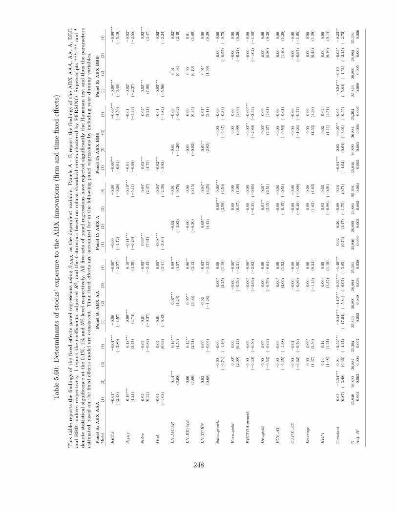
Tab
le5.60
:Determinants
ofstocks’
exposure
totheABX
innovations(firm
andtimefixed
effects)
This
table
reportsth
efindingsofth
efixed
effects
panel
regressionsusingβABX
asth
edep
enden
tvariable.PanelsA
-E
report
thefindingsofth
eABX
AAA,AA,A,BBB
andBBB-indices
resp
ectively.
Ireport
theco
efficien
ts,adjusted
R2,andth
et-statisticsbasedonrobust
standard
errors
clustered
byPERMNO.Superscripts
***,**and*
den
ote
statisticalsignifica
nce
atth
e0.1%,1%
and5%
level
resp
ectively.
Allfivesets
ofpanel
regressionshaverejected
significa
ntlyth
eHausm
antest
andthusth
eparameters
estimatedbasedonth
efixed
effects
model
are
consisten
t.Tim
efixed
effects
are
accountedforin
thefollowingpanel
regressionsbyincludingyea
rdummyvariables.
PanelA:ABX
AAA
PanelB:ABX
AA
PanelC:ABX
APanelD:ABX
BBB
PanelE:ABX
BBB-
Model
(1)
(2)
(3)
(4)
(1)
(2)
(3)
(4)
(1)
(2)
(3)
(4)
(1)
(2)
(3)
(4)
(1)
(2)
(3)
(4)
RET
t−0.01∗
−0.01∗∗
∗−0.00
−0.00∗
−0.00
−0.00
−0.00∗∗
∗−0.00∗∗
∗−0.00∗∗
∗−0.00∗∗
∗
(−2.43)
(−3.80)
(−1.57)
(−2.57)
(−1.72)
(−0.28)
(−6.01)
(−4.50)
(−6.40)
(−5.19)
βM
KT
0.19∗∗
∗0.18∗∗
∗0.09∗∗
∗0.10∗∗
∗−0.11∗∗
∗−0.10∗∗
∗−0.01
−0.01
−0.02∗
−0.02∗
(4.21)
(3.47)
(4.74)
(4.30)
(−6.29)
(−5.11)
(−0.69)
(−1.33)
(−2.37)
(−2.55)
Stdev
0.02
−0.04
−0.01
−0.05∗
0.09∗∗
∗0.04∗
0.02∗∗
∗0.02∗
0.03∗∗
∗0.02∗∗
∗
(0.52)
(−0.82)
(−0.37)
(−2.43)
(7.01)
(2.47)
(4.75)
(2.21)
(7.00)
(3.47)
IVol
−0.04
0.04
−0.01
0.05∗
−0.08∗∗
∗−0.04∗
−0.02∗∗
∗−0.01
−0.03∗∗
∗−0.02∗
(−1.03)
(0.93)
(−0.42)
(2.41)
(−5.84)
(−2.30)
(−3.83)
(−1.82)
(−5.56)
(−2.24)
LN
MCAP
0.14∗∗
∗0.19∗∗
∗0.07∗∗
∗0.08∗∗
∗−0.02
−0.01
−0.01
−0.00
0.01
0.02∗
(3.98)
(4.59)
(4.23)
(4.57)
(−1.83)
(−0.76)
(−1.26)
(−0.02)
(0.93)
(2.40)
LN
BE/M
E0.06
0.12∗∗
0.05∗∗
0.06∗∗
−0.00
0.00
−0.01
0.00
0.00
0.01
(1.60)
(2.71)
(3.06)
(3.13)
(−0.30)
(0.15)
(−0.92)
(0.35)
(0.70)
(1.89)
LN
TURN
0.02
−0.00
−0.02
−0.03∗
0.05∗∗
∗0.04∗∗
0.01∗∗
0.01∗
0.01∗
0.00
(0.68)
(−0.06)
(−1.28)
(−2.32)
(4.42)
(3.25)
(2.62)
(2.11)
(1.99)
(0.29)
Salesgrowth
−0.00
−0.00
0.00∗
0.00
0.00∗∗
∗0.00∗∗
∗−0.00
−0.00
−0.00
−0.00
(−0.74)
(−1.46)
(2.25)
(1.18)
(3.50)
(3.54)
(−0.47)
(−0.34)
(−0.57)
(−0.75)
Earn
yield
0.00∗
0.00
−0.00
−0.00∗
0.00
0.00
0.00
0.00
−0.00
0.00
(2.09)
(0.44)
(−0.59)
(−2.31)
(0.17)
(1.00)
(0.99)
(1.09)
(−0.24)
(0.29)
EBITDA
growth
−0.00
−0.00
−0.00∗
−0.00∗
−0.00
−0.00
−0.00∗∗
−0.00∗∗
∗−0.00
−0.00
(−0.60)
(−0.50)
(−2.09)
(−2.02)
(−0.35)
(−0.65)
(−2.80)
(−3.54)
(−1.04)
(−1.50)
Div
yield
−0.00
−0.00
−0.00
−0.00
0.01∗∗
0.01∗
0.00∗
0.00
0.00
0.00
(−0.53)
(−0.03)
(−0.79)
(−0.64)
(3.15)
(2.51)
(2.27)
(1.61)
(0.80)
(0.39)
FCF
AT
−0.00
−0.00
0.00∗
0.00
−0.00
−0.00
−0.00
−0.00
0.00
0.00
(−0.65)
(−1.38)
(2.00)
(1.52)
(−0.45)
(−0.51)
(−0.50)
(−0.01)
(1.10)
(1.25)
CAPX
AT
−0.00
−0.01
−0.00
−0.00
−0.00
−0.00
−0.00
−0.00
−0.00
−0.00
(−0.62)
(−0.76)
(−0.89)
(−1.06)
(−0.48)
(−0.88)
(−1.04)
(−0.77)
(−0.97)
(−1.05)
Lev
erage
0.00
0.00∗
−0.00
0.00
0.00
0.00
0.00
0.00
0.00
0.00
(1.67)
(2.56)
(−1.15)
(0.24)
(1.82)
(1.63)
(1.53)
(1.38)
(0.43)
(1.29)
BIG4
0.14
0.12
0.06
0.05
−0.03
−0.03
0.02
0.02
0.00
0.00
(1.48)
(1.21)
(1.32)
(1.10)
(−0.88)
(−0.91)
(1.11)
(1.51)
(0.16)
(0.14)
Constant
0.05
−1.54∗∗
∗0.04
−2.54∗∗
∗−0.44∗∗
∗−1.16∗∗
∗−0.33∗∗
∗−1.49∗∗
∗0.02
0.26
−0.08
0.16
−0.04∗∗
∗0.05
−0.05∗∗
−0.05
−0.04∗∗
∗−0.10
−0.03∗
−0.23∗∗
(0.87)
(−3.48)
(0.36)
(−4.47)
(−17.04)
(−5.84)
(−6.07)
(−5.85)
(0.76)
(1.47)
(−1.75)
(0.71)
(−4.62)
(0.64)
(−3.01)
(−0.55)
(−5.84)
(−1.51)
(−2.15)
(−2.72)
N35,846
26,890
26,884
25,304
35,846
26,890
26,884
25,304
35,846
26,890
26,884
25,304
35,846
26,890
26,884
25,304
35,846
26,890
26,884
25,304
Adj.
R2
0.003
0.003
0.004
0.007
0.052
0.039
0.036
0.038
0.003
0.003
0.002
0.004
0.005
0.005
0.004
0.006
0.009
0.005
0.003
0.006
248
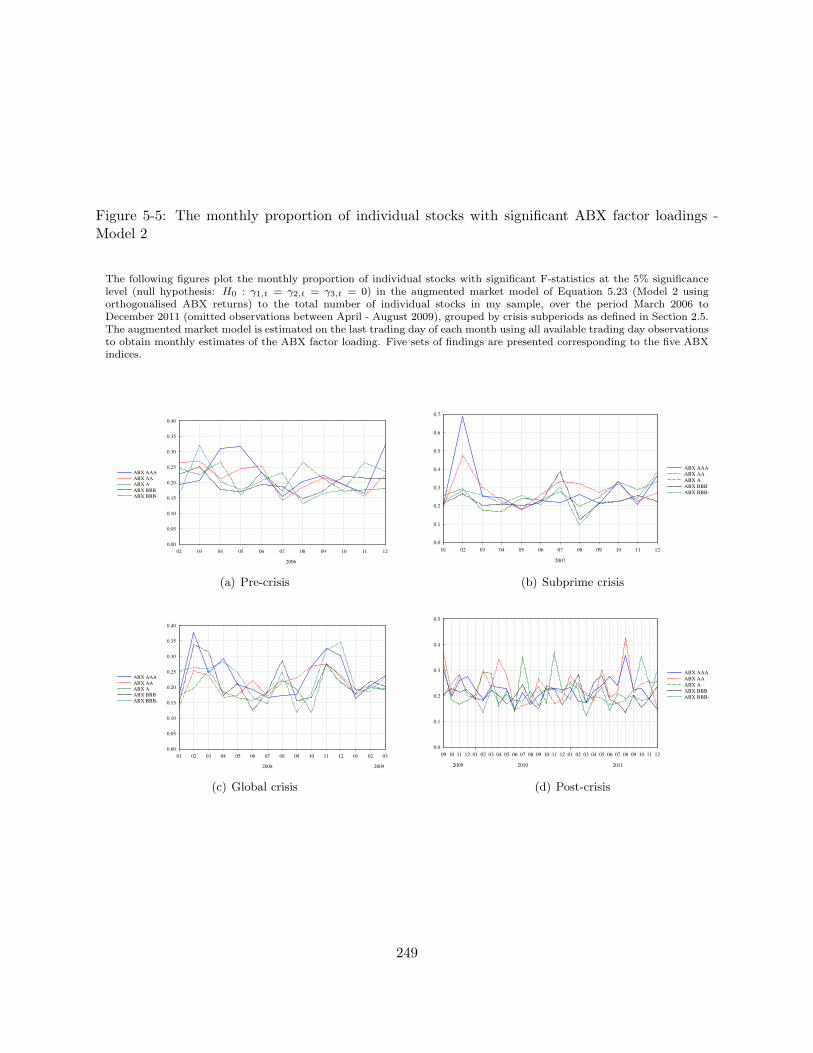
Figure 5-5: The monthly proportion of individual stocks with significant ABX factor loadings -Model 2
The following figures plot the monthly proportion of individual stocks with significant F-statistics at the 5% significancelevel (null hypothesis: H0 : γ1,t = γ2,t = γ3,t = 0) in the augmented market model of Equation 5.23 (Model 2 usingorthogonalised ABX returns) to the total number of individual stocks in my sample, over the period March 2006 toDecember 2011 (omitted observations between April - August 2009), grouped by crisis subperiods as defined in Section 2.5.The augmented market model is estimated on the last trading day of each month using all available trading day observationsto obtain monthly estimates of the ABX factor loading. Five sets of findings are presented corresponding to the five ABXindices.
0.00
0.05
0.10
0.15
0.20
0.25
0.30
0.35
0.40
02 03 04 05 06 07 08 09 10 11 12
2006
ABX AAA
ABX AA
ABX A
ABX BBB
ABX BBB-
(a) Pre-crisis
0.0
0.1
0.2
0.3
0.4
0.5
0.6
0.7
01 02 03 04 05 06 07 08 09 10 11 12
2007
ABX AAA
ABX AA
ABX A
ABX BBB
ABX BBB-
(b) Subprime crisis
0.00
0.05
0.10
0.15
0.20
0.25
0.30
0.35
0.40
01 02 03 04 05 06 07 08 09 10 11 12 01 02 03
2008 2009
ABX AAA
ABX AA
ABX A
ABX BBB
ABX BBB-
(c) Global crisis
0.0
0.1
0.2
0.3
0.4
0.5
09 10 11 12 01 02 03 04 05 06 07 08 09 10 11 12 01 02 03 04 05 06 07 08 09 10 11 12
2009 2010 2011
ABX AAA
ABX AA
ABX A
ABX BBB
ABX BBB-
(d) Post-crisis
249
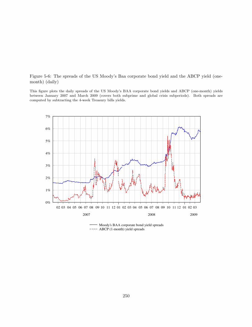
Figure 5-6: The spreads of the US Moody’s Baa corporate bond yield and the ABCP yield (one-month) (daily)
This figure plots the daily spreads of the US Moody’s BAA corporate bond yields and ABCP (one-month) yieldsbetween January 2007 and March 2009 (covers both subprime and global crisis subperiods). Both spreads arecomputed by subtracting the 4-week Treasury bills yields.
0%
1%
2%
3%
4%
5%
6%
7%
02 03 04 05 06 07 08 09 10 11 12 01 02 03 04 05 06 07 08 09 10 11 12 01 02 03
2007 2008 2009
Moody’s BAA corporate bond yield spreads
ABCP (1-month) yield spreads
250
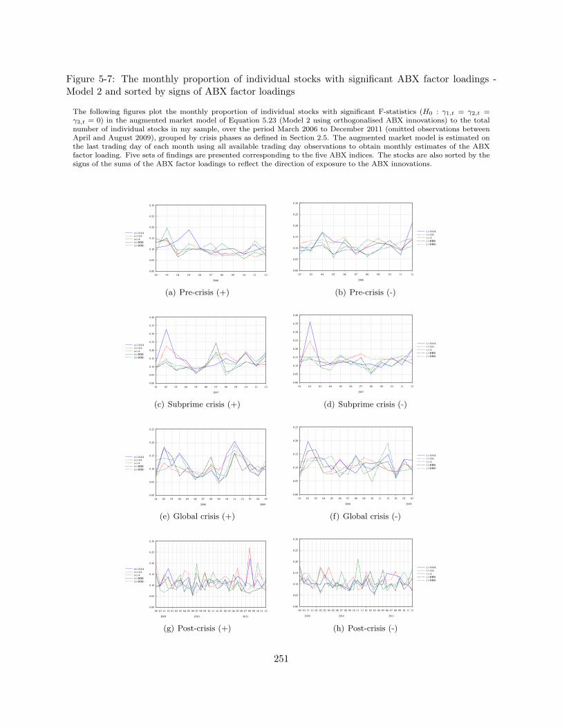
Figure 5-7: The monthly proportion of individual stocks with significant ABX factor loadings -Model 2 and sorted by signs of ABX factor loadings
The following figures plot the monthly proportion of individual stocks with significant F-statistics (H0 : γ1,t = γ2,t =γ3,t = 0) in the augmented market model of Equation 5.23 (Model 2 using orthogonalised ABX innovations) to the totalnumber of individual stocks in my sample, over the period March 2006 to December 2011 (omitted observations betweenApril and August 2009), grouped by crisis phases as defined in Section 2.5. The augmented market model is estimated onthe last trading day of each month using all available trading day observations to obtain monthly estimates of the ABXfactor loading. Five sets of findings are presented corresponding to the five ABX indices. The stocks are also sorted by thesigns of the sums of the ABX factor loadings to reflect the direction of exposure to the ABX innovations.
0.00
0.05
0.10
0.15
0.20
0.25
0.30
02 03 04 05 06 07 08 09 10 11 12
2006
(+) AAA
(+) AA
(+) A
(+) BBB
(+) BBB-
(a) Pre-crisis (+)
0.00
0.05
0.10
0.15
0.20
0.25
0.30
02 03 04 05 06 07 08 09 10 11 12
2006
(-) AAA
(-) AA
(-) A
(-) BBB
(-) BBB-
(b) Pre-crisis (-)
0.00
0.05
0.10
0.15
0.20
0.25
0.30
0.35
0.40
01 02 03 04 05 06 07 08 09 10 11 12
2007
(+) AAA
(+) AA
(+) A
(+) BBB
(+) BBB-
(c) Subprime crisis (+)
0.00
0.05
0.10
0.15
0.20
0.25
0.30
0.35
0.40
01 02 03 04 05 06 07 08 09 10 11 12
2007
(-) AAA
(-) AA
(-) A
(-) BBB
(-) BBB-
(d) Subprime crisis (-)
0.00
0.05
0.10
0.15
0.20
0.25
01 02 03 04 05 06 07 08 09 10 11 12 01 02 03
2008 2009
(+) AAA
(+) AA
(+) A
(+) BBB
(+) BBB-
(e) Global crisis (+)
0.00
0.05
0.10
0.15
0.20
0.25
01 02 03 04 05 06 07 08 09 10 11 12 01 02 03
2008 2009
(-) AAA
(-) AA
(-) A
(-) BBB
(-) BBB-
(f) Global crisis (-)
0.00
0.05
0.10
0.15
0.20
0.25
0.30
09 10 11 12 01 02 03 04 05 06 07 08 09 10 11 12 01 02 03 04 05 06 07 08 09 10 11 12
2009 2010 2011
(+) AAA
(+) AA
(+) A
(+) BBB
(+) BBB-
(g) Post-crisis (+)
0.00
0.05
0.10
0.15
0.20
0.25
0.30
09 10 11 12 01 02 03 04 05 06 07 08 09 10 11 12 01 02 03 04 05 06 07 08 09 10 11 12
2009 2010 2011
(-) AAA
(-) AA
(-) A
(-) BBB
(-) BBB-
(h) Post-crisis (-)
251
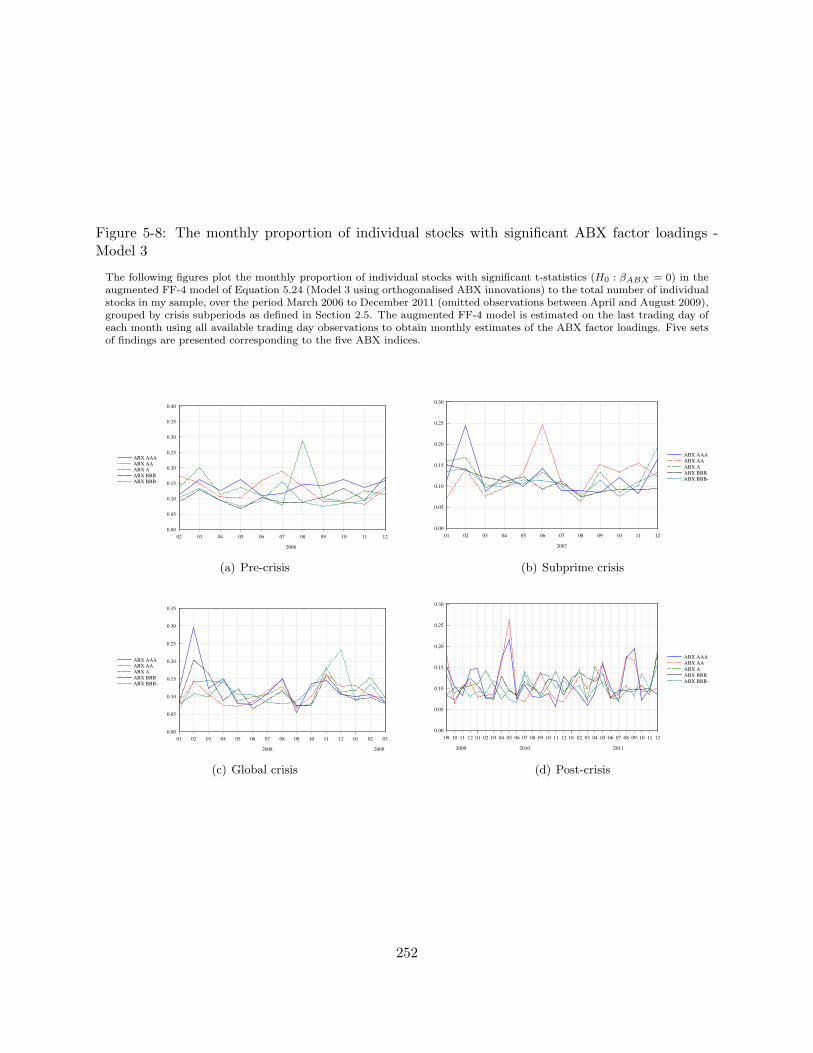
Figure 5-8: The monthly proportion of individual stocks with significant ABX factor loadings -Model 3
The following figures plot the monthly proportion of individual stocks with significant t-statistics (H0 : βABX = 0) in theaugmented FF-4 model of Equation 5.24 (Model 3 using orthogonalised ABX innovations) to the total number of individualstocks in my sample, over the period March 2006 to December 2011 (omitted observations between April and August 2009),grouped by crisis subperiods as defined in Section 2.5. The augmented FF-4 model is estimated on the last trading day ofeach month using all available trading day observations to obtain monthly estimates of the ABX factor loadings. Five setsof findings are presented corresponding to the five ABX indices.
0.00
0.05
0.10
0.15
0.20
0.25
0.30
0.35
0.40
02 03 04 05 06 07 08 09 10 11 12
2006
ABX AAA
ABX AA
ABX A
ABX BBB
ABX BBB-
(a) Pre-crisis
0.00
0.05
0.10
0.15
0.20
0.25
0.30
01 02 03 04 05 06 07 08 09 10 11 12
2007
ABX AAA
ABX AA
ABX A
ABX BBB
ABX BBB-
(b) Subprime crisis
0.00
0.05
0.10
0.15
0.20
0.25
0.30
0.35
01 02 03 04 05 06 07 08 09 10 11 12 01 02 03
2008 2009
ABX AAA
ABX AA
ABX A
ABX BBB
ABX BBB-
(c) Global crisis
0.00
0.05
0.10
0.15
0.20
0.25
0.30
09 10 11 12 01 02 03 04 05 06 07 08 09 10 11 12 01 02 03 04 05 06 07 08 09 10 11 12
2009 2010 2011
ABX AAA
ABX AA
ABX A
ABX BBB
ABX BBB-
(d) Post-crisis
252
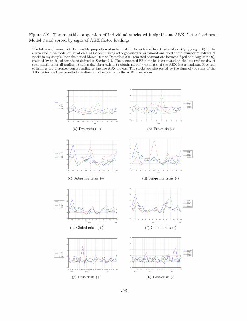
Figure 5-9: The monthly proportion of individual stocks with significant ABX factor loadings -Model 3 and sorted by signs of ABX factor loadings
The following figures plot the monthly proportion of individual stocks with significant t-statistics (H0 : βABX = 0) in theaugmented FF-4 model of Equation 5.24 (Model 3 using orthogonalised ABX innovations) to the total number of individualstocks in my sample, over the period March 2006 to December 2011 (omitted observations between April and August 2009),grouped by crisis subperiods as defined in Section 2.5. The augmented FF-4 model is estimated on the last trading day ofeach month using all available trading day observations to obtain monthly estimates of the ABX factor loadings. Five setsof findings are presented corresponding to the five ABX indices. The stocks are also sorted by the signs of the sums of theABX factor loadings to reflect the direction of exposure to the ABX innovations.
0.00
0.04
0.08
0.12
0.16
0.20
02 03 04 05 06 07 08 09 10 11 12
2006
(+) AAA
(+) AA
(+) A
(+) BBB
(+) BBB-
(a) Pre-crisis (+)
0.00
0.04
0.08
0.12
0.16
0.20
02 03 04 05 06 07 08 09 10 11 12
2006
(-) AAA
(-) AA
(-) A
(-) BBB
(-) BBB-
(b) Pre-crisis (-)
0.02
0.04
0.06
0.08
0.10
0.12
0.14
01 02 03 04 05 06 07 08 09 10 11 12
2007
(+) AAA
(+) AA
(+) A
(+) BBB
(+) BBB-
(c) Subprime crisis (+)
0.02
0.04
0.06
0.08
0.10
0.12
0.14
01 02 03 04 05 06 07 08 09 10 11 12
2007
(-) AAA
(-) AA
(-) A
(-) BBB
(-) BBB-
(d) Subprime crisis (-)
0.00
0.04
0.08
0.12
0.16
0.20
01 02 03 04 05 06 07 08 09 10 11 12 01 02 03
2008 2009
(+) AAA
(+) AA
(+) A
(+) BBB
(+) BBB-
(e) Global crisis (+)
0.00
0.04
0.08
0.12
0.16
0.20
01 02 03 04 05 06 07 08 09 10 11 12 01 02 03
2008 2009
(-) AAA
(-) AA
(-) A
(-) BBB
(-) BBB-
(f) Global crisis (-)
0.00
0.04
0.08
0.12
0.16
0.20
09 10 11 12 01 02 03 04 05 06 07 08 09 10 11 12 01 02 03 04 05 06 07 08 09 10 11 12
2009 2010 2011
(+) AAA
(+) AA
(+) A
(+) BBB
(+) BBB-
(g) Post-crisis (+)
0.00
0.04
0.08
0.12
0.16
0.20
09 10 11 12 01 02 03 04 05 06 07 08 09 10 11 12 01 02 03 04 05 06 07 08 09 10 11 12
2009 2010 2011
(-) AAA
(-) AA
(-) A
(-) BBB
(-) BBB-
(h) Post-crisis (-)
253

THIS PAGE INTENTIONALLY LEFT BLANK
254
Chapter 6
The Determinants of Bank Equity
Risks
6.1 Introduction
In the US banking sector, anecdotal evidence shows that bank risk taking is associated with man-
agerial shareholdings (Demsetz et al., 1997; Anderson and Fraser, 2000), the presence of capital
adequacy requirements (Konishi and Yasuda, 2004), board structure and CEO power (Pathan,
2009), and franchise value (Keeley, 1990; Demsetz et al., 1997; Anderson and Fraser, 2000). While
the majority of bank risk studies are motivated from a corporate governance perspective, given the
relative importance of firms’ fundamental characteristics in explaining equity risk53, it is surprising
that the role of fundamental variables in explaining bank risk has not yet been fully explored.54
Given the profound changes to the US banking system and the growing importance of securitisa-
tion to banks’ risk management over the past decade, the US bank risk literature requires some
updating.
53Evidence of cross-sectional and time series relations between return volatilities and firms’ characteristics has beendocumented; for example, return on equity (Wei and Zhang, 2006), earnings growth, institutional ownership (Xu andMakiel, 2003), and dividend yield (Pastor and Veronesi, 2003).
54Stiroh (2006) finds evidence that the US BHCs’ operating choice and non-interest generating activities affect bankequity risks over the 1997 to 2004 period. The author (p. 245) makes it clear that the objective of his investigationis to find out ‘how differences in ex ante operating choices, captured by cross-sectional differences in balance sheetand income statements, are linked to the volatility of future returns’. The objective of this study differs in twomajor ways. First, I study the within-bank relation between the banks’ fundamental characteristics and the bankequity risks (i.e. the within-effects). Second, this chapter focuses on the changes in the impact of the fundamentalcharacteristics on bank risks during the recent crisis. The implications in this study are mainly offered to shareholdersand bondholders in the context of investment and risk management as well as bank regulators in relation to banks’exposure to funding illiquidity risks.
255
The recent 2007 to 2009 financial crisis highlights the tragic consequences of banks’ excessive risk
taking and brings to light the banks’ vulnerability to systematic funding illiquidity shocks (Gorton,
2009). The understanding of the fundamental sources of bank equity risks during the recent crisis
offers important policy implications to bank regulators in relation to the effectiveness of the existing
tools in monitoring and regulating banks’ risk, and to a range of market participants that include
shareholders, bondholders, borrowers, etc. Following prior literature (see, for example, Anderson
and Fraser, 2000; Stiroh, 2006; Haq and Heaney, 2012), this study utilises market-based equity
risk and unravels the fundamental sources of bank risks. Specifically, I investigate the impact of
bank opacity, profitability, loan portfolio asset quality and capital adequacy on various components
of bank risks (market, interest rate, crisis-related, funding illiquidity, market wide default and
idiosyncratic risks) and focus on their interactions during the crisis.
In the US ‘shadow’ banking system there is a maturity mismatch feature in that banks issue
short-term ABCP to finance long-term structured finance securities via off-balance sheet conduits
(see, Eichengreen, 2008; Frank et al., 2008; Brunnermeier, 2009; Acharya et al., 2013). During the
recent crisis, the banks reluctantly provided contingent liquidity to the conduits via their credit line
facilities and were susceptible to considerable funding illiquidity risks. I consider banks’ exposure
to funding illiquidity risks as a source of bank risks in my variance decomposition and study its
determinants. Improved understanding of the fundamental sources of banks’ funding illiquidity
risks is of utmost importance to regulators in measuring banks’ exposure to systemic risks and
guiding the development of effective regulatory risk measurement and management tools.
As pointed out by a number of researchers (see, for example, Benmelech and Dlugosz, 2009;
Brunnermeier, 2009; Gorton, 2009; Mahlmann, 2013), securitised and structured finance products
(e.g., the CDOs and subprime RMBS) are responsible for the intensification of the recent crisis.
As downgrades of these structured securities spiked in 2007 (Benmelech and Dlugosz, 2009), the
structured finance securities’ prices plunged (for losses on RMBS, see, Merrill et al., 2012). The
structured finance market is shown empirically to be the origin of contagion and thus represents
a source of considerable risk during the crisis (Fender and Scheicher, 2009; Longstaff, 2010; see
Chapter 5). Banks were essentially subject to the spillovers of shocks that constitute a formidable
source of bank risk during the crisis. To this end, I depart from the prior literature and consider
a crisis-related component of bank equity risks that reflects the degree of BHCs’ exposure to the
troubled structured finance market.55 The evidence in this study shows that banking firms with
weaker fundamentals were more vulnerable to contagion during the crisis.
An important fundamental variable I consider is the banks’ asset composition. It has been
55The structured finance market is measured by the ABX AAA index, a benchmark index which tracks the per-formance of a static portfolio of subprime RMBS).
256

widely acknowledged that banks are more opaque than non-banks given their unique role of dele-
gated monitoring. The main source of opacity pertains to investors’ informational asymmetry in
evaluating the credit quality of banks’ loan assets which are not fully disclosed. Asset composition
is a major determinant of bank opacity because banks’ investment in opaque assets is relatively
harder for analysts to value, resulting in a larger degree of disagreement in valuation amongst
credit rating agencies (Morgan, 2002; Iannotta, 2006, Flannery et al., 2013). Evidence shows that
investors insufficiently discount risks in banks’ opaque investments, which are then rewarded with
higher market valuation leading to higher systematic risk and lower idiosyncratic risk (Jones et
al., 2013).56 To my knowledge, the role of banks’ opacity in explaining bank risks has not been
fully examined in the literature.57 To fill this gap, I test whether banks’ exposure to opaque assets
contributes positively to bank equity risks.
This chapter makes several important contributions to the existing bank risk literature. First
of all, this study seeks to identify the fundamental sources of bank risks by investigating the de-
terminants of the market-based bank equity risks using a diverse set of bank-specific fundamental
characteristics that include banks’ profitability (earnings and non-interest income), loan portfolio
credit quality (non-performing loans)58, Tier 1 capital ratios, loan-to-deposit ratios and various
control variables. This chapter establishes empirically the link between banks’ fundamental and
equity risks and offers insight to investors in the context of asset valuation by highlighting the sub-
stantive relevance of fundamental analysis in evaluating bank stocks’ risk and return relationship.
Second, I inquire whether the recent financial crisis has had any effects on the impact of banks’
fundamental variables on bank equity risks; that is, whether the relevance of some banks’ funda-
mental characteristics have become stronger. In doing so, I provide useful implications to market
users in the context of investment management during a crisis period characterised by increasing
macroeconomic risks and risk aversion. Third, specific to the context of the recent crisis, I am the
first to consider banks’ exposure to the troubled structured finance market and the asset-backed
money market (ABCP) as constituents of bank equity risks. The identification of the fundamental
determinants of banks’ exposure to the shocks originated from these markets has important policy
implications in relation to the quantification and the regulation of banks’ systemic risks. Fourth,
to my knowledge, I am the first to examine directly the relation between bank opacity, as measured
by the banks’ asset composition, and equity risks in the US banking sector and to examine its
56Jones et al. (2013) argue that bank opacity hinders the effectiveness of market discipline to price risks andtranslates into higher risk of systemic failure.
57Stiroh (2006) finds evidence that banks’ lending activities determine banks risks. However, the author does notexplicitly test for the effects of asset opaqueness on bank risks.
58Non-performing loans to total assets have been studied by Stiroh (2006) as control variables for bank totalrisks. Haq and Heaney (2012) consider banks’ credit risk, measured by the loan-loss provision to total asset andnon-performing loans to total assets but do not consider non-performing loans as determinants of bank risks.
257
interaction during the crisis. Lastly, this study contributes to the literature on bank liquidity risk
management by allowing us to test explicitly whether banks’ buffer of Tier 1 capital reduces banks’
exposure to market wide funding illiquidity shocks. The evidence in this study justifies the urge
for higher regulatory capital requirements in limiting banks’ exposure to systemic risks.
Using pooled weighted least squares (WLS) regressions with two-way fixed effects, I quantify
the impact of bank opacity and banks’ fundamental characteristics on the various components of
bank equity risks and specifically examine their interactions during the recent crisis. I find evidence
that banks’ exposure to various trading and loan assets contributes significantly and positively to
the banks total and idiosyncratic risks in the non-crisis subsample.59 However, little evidence of
significant differences between the impact of opaque and transparent assets on bank equity risks is
documented. Asset opaqueness in general does not contribute to bank equity risks consistent with
Jones et al. (2013) in that the riskiness of banks’ investment in opaque assets were insufficiently
discounted and inaccurately priced. The impact of asset composition on bank risks has in general
become negative during the crisis, suggesting some structural changes in the perceived riskiness of
banks’ lending activities by the market. More importantly, my study documents reasonably strong
evidence that the banks’ earnings to total assets and Tier 1 capital ratios determine (negative re-
lation) significantly bank equity risks. Banks with higher profitability and larger buffer of Tier 1
capital have significantly lower bank equity risks in both the non-crisis and crisis subsamples. In
addition, while the impact of non-performing loans on the bank equity risks was insignificant during
the non-crisis subsample, its impact on banks’ total, market wide default and idiosyncratic risks in-
creased by threefold. Banks’ loan portfolio credit quality has become the most relevant fundamental
risk factors to asset valuation when the crisis unfolded. Banks with poorer loan portfolio credit
quality suffered higher return volatilities and were more exposed to the heightening market wide
default risks, particularly during the crisis. From an investor’s perspective, the empirical relation
between banks’ fundamental and equity risks highlights the important role of banks’ fundamental
characteristics in evaluating bank stock performance. In addition, this paper documents a strong
and negative empirical relation between banks’ Tier 1 capital ratios and the degree of banks’ expo-
sure to the unexpected shocks from the US structured finance market and the asset-backed money
market. The evidence implies that banks’ buffer of Tier 1 capital is an effective shield against the
contagion-related spillovers of shocks and against the funding illiquidity risks.
This chapter relates closely to a number of papers that examine bank performance during the
financial crisis. Fahlenbrach et al. (2012) compare banks’ performance during the 1998 and the
recent 2007 to 2009 financial crises, and find that banks with higher exposure to illiquid assets and
leverage under-performed during the recent crisis. Acharya et al. (2013) study banks’ issuance of
59Throughout the study, I use the terms residual risks, firm-specific risks and idiosyncratic risks interchangeably.
258

ABCP and find that banks with higher exposure to ABCP conduits had lower returns. Beltratti
and Stulz (2012), based on cross-country evidence, find that large banks’ under-performance during
the 2007 to 2008 period is related to their reliance on short-term funds and their funding fragility
in relation to capital adequacy and deposit. A number of papers present evidence that corporate
governance practices played little role in explaining the under-performance of bank stocks, for
example: better alignment of CEO incentives with shareholders performed worse (Fahlenbrach
and Stulz, 2011), banks with more shareholder-friendly boards under-performed (Beltratti and
Stulz, 2012), etc. The evidence in this study supplements the findings of these papers and further
reveals that banks’ under-performance during the crisis is related to banks’ fundamental risks
pertaining to profitability, loan portfolio asset quality, funding illiquidity risks and lending activities.
The findings in this study also lend support to the fundamentalist view that banks’ fundamental
performance is crucial in explaining stock performance with profound implications to shareholders
and bondholders. From a supervisory perspective, this study shows that one major source of bank
equity risk is banks’ vulnerability to funding illiquidity shocks, which is fundamentally determined
by banking firms’ degree of capital adequacy. The evidence in this study provides empirical support
to the urge for higher regulatory capital requirement in preventing systemic failure in light of market
wide funding illiquidity.
The remainder of this chapter is organised as follows. Section 2 discusses my motivation and
explains my hypotheses. Section 3 explains my data and empirical framework. Section 4 reports
my empirical results and Section 5 concludes.
6.2 Motivation and hypotheses
6.2.1 Bank opacity
It is commonly acknowledged in the prior literature that banks are more opaque than non-banks
(Morgan, 2002). The opacity lies on the notion of informational asymmetry arising in a number
of ways. First, asymmetric information arises from the relative difficulty in valuing banking firms’
assets when banking firms, as the delegated monitors, have privileged knowledge on loans’ credit
qualities and do not fully disclose this information. In addition, the banks might understate their
losses during worsening financial conditions (Gunther and Moore, 2003) or smooth their earnings
(Bhat, 1996; Fonseca and Gonzalez, 2008). The lack of transparency and the potential problems
of moral hazard are the fundamental causes of bank opacity. Second, bank opacity arises from
the opaqueness of its trading assets (Jones et al., 2013). Morgan (2002) points out that trading
assets are more liquid and may be easier to ‘slip’ in and out of the financial statements at banks’
259
discretion given the mark-to-market accounting treatment. As a result, the wider scope for banks
to manipulate the amount of booked trading assets gives rise to the banks’ relative opacity to non-
banks. Third, the banks’ issuance of opaque securitised financial products (e.g. ABS, collateralised
mortgage obligations (CMO) and CDOs) via off-balance sheet conduits increased drastically over
the past two decades (Weaver, 2008; Brunnermeier, 2009). Since the structured securities are in
general hard-to-value and are nontransparent, their valuation became extremely difficult during
the crisis, resulting in considerable uncertainty and opacity amongst banking firms.
Asset composition is a major determinant of bank opacity. On the empirical side, the banks’
loans and financial assets are important sources of disagreement amongst bond rating agencies,
with split ratings more likely for banks consistent with higher relative opacity (Morgan, 2002;
Iannotta, 2006). The underlying argument pertains to the stylised fact that banks’ investments in
opaque assets are relatively harder for analysts or rating agencies to evaluate. Asset composition
may affect bank risks in the context of bank opacity in three ways. First, Jones et al. (2013)
show that the banks’ investments in opaque assets are related to higher systematic risks and lower
idiosyncratic risks over time as a result of inefficient market discipline in pricing risks. I put forward
this contention and test explicitly the relation between asset opaqueness and bank risks. Second,
some types of bank assets may be more cross-correlated and have a lower degree of diversification
than other asset types. For instance, banks’ trading assets (e.g. subprime related CDOs), which are
shown in hindsight to be highly correlated across securitised tranches as a result of wrong actuarial
assumptions (Jaffe, 2008; Weaver, 2008) and over-reliance on rating agencies (Partnoy, 2009). The
banks’ exposure to these assets may pose a higher risk to individual banks in terms of solvency
and contribute to bank equity risks.60 Third, during the recent crisis, banks with more investments
in hard-to-value assets may be prone to receiving rating downgrades and write-offs, and are thus
more subject to risks in relation to funding illiquidity and insolvency. While return volatilities
are determined by public information (Jones et al., 1994) and the risks embedded in the opaque
assets were not fully priced by investors before the crisis (Jones et al., 2013), the investors received
wake-up calls and systematically sold from these bank stocks, resulting in tremendous downward
price pressure. Bank asset opaqueness may have become increasingly relevant to investors during
the crisis as an indicator of risk.
From my discussion above, I advance three hypotheses centering on the notion of bank opacity,
measured by asset composition. Hypothesis 1A asserts that banks’ asset composition significantly
explains the bank risks. Hypothesis 1B alleges that banks’ investments in more opaque assets
60On the other hand, a competing argument by Flannery et al. (2004) states that bank opacity may not affectreturn volatilities. The argument states that since the impact of changes in true values of the assets on stock returnsare only available publicly on a quarterly basis, the asset price volatilities are low between information arrival datesand that asset price changes only when information reaches the market.
260
have a stronger positive impact on bank risks than those of the transparent assets. Hypothesis 1C
contends that the impact of asset composition on bank risks differs across the non-crisis and crisis
subsamples.
6.2.2 Structured finance market failure and banks’ funding illiquidity risk
Brunnermeier (2009) points out that the ‘shadow’ banking system and the process of securiti-
sation have both contributed to the severity of the recent crisis. Within the ‘shadow’ banking
system, banks are incentivised to issue and underwrite excessively complex and opaque structured
finance securities using off-balance sheet conduits as means of risk transfer and regulatory arbitrage
(Acharya et al., 2013). The off-balance sheet SIVs carry the same maturity mismatch feature as
in the traditional banking model and usually rely on the issuance of short-term ABCP to finance
the purchases of longer term assets, such as ABS and CDOs (Eichengreen, 2008, and Frank et al.,
2008). Since banking firms were liable for the credit lines granted to the off-balance sheet SIVs,
they were exposed to considerable funding illiquidity risk as investors were unwilling to roll over
the short-term money market instruments during the crisis.61
The banking firms’ vulnerability to the shocks from the asset-backed money markets and the
troubled structured finance market highlights the importance of effective and timely liquidity risk
management. Cornett et al. (2011) find empirically that the four main drivers of liquidity risk
in modern banks are the changes in banking firms’ core deposits, liquid assets, equity capital and
exposure to loan commitments. The authors show that it is the core deposits rather than total
deposits that stabilise the liquidity supply and that the core deposits and originated loans increased
during the time when the market liquidity of bank assets was low. Banking firms’ equity capital
is of importance to liquidity management since it serves as a buffer that protects depositors from
liquidity shocks and helps absorb risk at large banks (Diamond and Rajan, 2000; Berger and
Bouwman, 2012). Based on the evidence and theoretical arguments, I argue that banks’ equity
capital, core deposit and total loans contain important information that reflect the underlying
fundamental risks and thus the equity risks. To this end, I include the ratios of total loan to total
core deposits to gauge the banks’ ability to meet funding demands, the Tier 1 capital ratio as a
measure of banks’ equity capital in buffering funding illiquidity shocks, and the ratio of total core
deposits to total assets as a control variable for the supply of retail deposits. Hypothesis 2A asserts
61Acharya et al. (2013) find that the liquidity guarantees on the ABCP were concentrated in the ABCP conduitssponsored by commercial banks. The authors conclude that banks did not securitise for risk transferring but ratherfor regulatory arbitrage purposes (i.e. to reduce the base of risk weighted assets), especially amongst banks with lesscapital. The authors find that stock returns were lower for banks with higher exposure to the ABCP conduits duringthe recent crisis and that losses in conduits were borne by banks. The evidence suggests that banks’ exposure tofunding illiquidity risks was at least in part priced in the market, lending support to my conjecture.
261
that banks’ funding ability and capital adequacy are related negatively to bank equity risks. To
test whether their relevance to explaining bank equity risks might have elevated during the crisis,
Hypothesis 2B asserts that their impact on bank equity risks strengthened became more negative
during the crisis.
6.2.3 Profitability, loan portfolio credit quality and bank risks
Evidence in support of a negative relation between earnings and return volatilities has been docu-
mented in the literature. Wei and Zhang (2006) argue that the firms’ return on equity and variances
of return on equity are integral parts of their conditional volatilities and find evidence that return on
equity explains stock return volatilities in both time-series and cross-sectional dimensions. Likewise,
Cooper et al. (2003) examine bank stock returns and document significant return predictability
in the quarterly changes of banks’ earning per share, leverage, loan loss reserve and non-interest
income within an asset pricing framework.
The evidence suggests that banks’ profitability and loan portfolio credit quality might have
contained important information with regard to banks’ operating performance and fundamental
risks that impact on bank stock performance and bank equity risks. Hypothesis 3A asserts that
banks’ profitability, measured by earnings to total assets, contributes negatively to bank risks
while Hypothesis 4A contends that banks with better loan portfolio credit quality, measured by the
amount of non-performing loans, have lower risks.62 Hypotheses 3B and 4B assert that the impact
of banks’ profitability and loan portfolio credit quality on bank risks have increased, respectively,
during the crisis.
6.3 Data and empirical approach
My sample consists of all publicly available traded US BHCs, with $500 million or more consolidated
assets, that file FR Y-9C forms with the Federal Reserve quarterly over the sample period from
2006Q1 to 2011Q4. All the companies’ quarterly consolidated fundamental and financial data
are obtained via the Bank Regulatory database in the Wharton Research Data Services (WRDS)
Database. The quarterly fundamental data are merged with the market data from the CRSP
database63 by PERMCO and RSSD ID64 and with the linking table provided by the New York
62Stiroh (2006) finds evidence that non-performing loans to total assets is positively related to banks’ total risks.Meeker and Gray (1987) show that the amount of non-performing loans are satisfactory measures of bank assetquality.
63Similar to Anderson and Fraser (2000), I include stocks with SIC codes: 6021 (National commercial banks), 6022(State commercial banks), 6029 (Commercial banks, NEC) from CRSP.
64PERMCO is the CRSP unique company identifier while RSSD is the unique bank identifier on the Bank Regu-latory database (the variable is RSSD9001).
262
Federal Reserve Bank (FRB)65. I screen out those quarterly observations in which there are missing
or unmerged data to 227 BHC and 3447 bank-quarters. The total assets are adjusted for inflation
using a seasonally-adjusted GDP deflator with a base price level of 2005.
Following Jones et al. (2013), all balance sheet variables are calculated as the quarterly averages
of the beginning and ending values of quarter t while the income measures are annualised quarterly
amounts. Variable names that start with “LN ” or end with “ A” refer to those variables that
are log transformed or normalised by the total assets respectively. To reduce the potential bias
due to outliers, all bank variables have been winsorised at the 99th percentile (1% at each tail)
at each cross-section. In addition, to ensure that I am capturing genuine causal relations and to
lessen potential endogeneity problems, all independent variables in the regressions are lagged by
one quarter.
6.3.1 The ABX indices
Evidence of contagion travelling from the US structured finance market to domestic US markets
has been documented during the recent crisis (Longstaff, 2010; Chapters 4 and 5). The unexpected
shock components of the structured finance market represent a source of crisis-related risk during
the subprime crisis (Fender and Scheicher, 2009; Chapter 5). To account for the relative importance
of the crisis-specific risks, I consider a bank equity risk component related to the innovations in the
ABX index.
Since its index initialisation in 2006, the ABX index family has become an important type of
stress barometer for subprime RMBS market conditions (Fender and Scheicher, 2009). The ABX
indices, maintained by MARKIT, are equally-weighted and static portfolios that each reference 20
subprime RMBS deals. The indices serve as benchmarks of the structured finance market in which
the securities are collateralised by subprime home loans. Five ABX indices, corresponding to the
AAA, AA, A, BBB and BBB- credit ratings of the underlying RMBS deals, are maintained.66 For
the purpose of the analysis in this chapter, the ABX index of the ABX.HE.06-1 vintage, which was
issued in January 2006 and has the longest historical data, is included for the variance decomposition
of bank equity risks. As shown in Fig. 4-1 of Chapter 4, the prices of the five ABX indices of the
ABX HE.06-1 vintage all started to fall in early 2007 and declined sharply from mid 2007 till mid
2009. The ABX AAA index outperformed the rest of the ABX indices and was the most resilient
after the recent crisis. In addition, the evidence presented in Chapter 5 shows that the ABX AAA
innovations were the most relevant in asset pricing compared to the remaining four ABX indices
and, hence, I include the ABX AAA index in the decomposition of bank equity risks and study its
65The linking table can be accessed via: http://www.newyorkfed.org/research/banking research/datasets.html66For more details on the ABX indices, please refer to Section 4.3 of Chapter 4.
263
determinants.
6.3.2 Decomposing bank equity risks
Following the variance decomposition approach in prior literature (see, Anderson and Fraser, 2000;
Pathan, 2009; Haq and Heaney, 2012), I decompose bank risks into six components, which are:
market, interest rate, the crisis-related (ABX), funding illiquidity (ABCP), default spread and
residual risks. I am the first to evaluate the determinants of the banks’ crisis-related (ABX) risk
and funding illiquidity (ABCP) risk using the banks’ fundamental variables, and to investigate
whether there is any impact of the recent 2007 to 2009 financial crisis on the explanatory power of
fundamental variables on bank equity risks.
To this end, I estimate multifactor models for each BHC using all available daily observations
of excess returns in each quarter. In particular, to separate the effects of each factor variable from
each other, I apply an orthogonalisation to the model and decompose the six risk components,
based on the following empirical approach:
1. Using all daily observations in each quarter, I orthogonalise the factor variables by running
the following regressions in order:
INTt =α+ βRMKT,t + ϵINT,t (6.1)
RABX,t =α+ βRMKT,t + ϵINT,t + ϵABX,t (6.2)
ABCPt =α+ βRMKT,t + ϵINT,t + ϵABX,t + ϵABCP,t (6.3)
DEFt =α+ βRMKT,t + ϵINT,t + ϵABX,t + ϵABCP,t + ϵDEF,t, (6.4)
where RMKT,t is the daily excess returns of the value-weighted CRSP market index, INTt is
the daily yield of the 3-month Treasury bills, RABX,t is the daily excess returns of the ABX
AAA index, ABCPt is the daily yield spreads of the one-month ABCP above the one-month
Treasury bill rates, and DEFt is the default spreads between the Moody’s AAA and BAA
corporate bond yields.
2. I obtain and use the factor variable innovations (ϵ), which represent the unexpected com-
ponents of the factor variables (i.e. shocks) to estimate the multifactor model for the ith
BHC:67
Rit = αi + βiRMKT,t + γi1ϵINT,t + γi2ϵABX,t + γi3ϵABCP,t + γi4ϵDEF,t + εit, (6.5)
67I screen out those BHCs with less than 30 daily observations in any quarters in estimating Equation 9.3.
264
where Rit is the daily excess returns of the ith BHC.
3. Since the factor variables are orthogonal to each other, the variance decomposition is straight-
forward:
σ2i = β2i σ2MKT + γ2i,1σ
2ϵINT
+ γ2i,2σ2ϵABX
+ γ2i,3σ2ϵABCP
+ γ2i,4σ2ϵDEF
+ σ2ε , (6.6)
where the σ2i , σ2ϵINT
, σ2ϵABX, σ2ϵABCP
, σ2ϵDEFand σ2ε refer to the variances68 of the excess
returns of the ith BHC, market index, innovations of the US interest rate, ABX index, ABCP
yield spreads, default spreads and the residuals of Equation 9.3, respectively, based on daily
observations over each quarter.
4. The risk measures (quarterly equivalent) for each BHC and each quarter are then computed
as:
σTOTALi = σi ×
√T , (6.7)
σMKTi =
√β2i σ
2MKT ×
√T , (6.8)
σINTi =
√γ2i,1σ
2ϵINT
×√T , (6.9)
σABXi =
√γ2i,2σ
2ϵABX
×√T , (6.10)
σABCPi =
√γ2i,3σ
2ϵABCP
×√T , (6.11)
σDEFi =
√γ2i,4σ
2ϵDEF
×√T , (6.12)
σRESIDi = σεi ×
√T , (6.13)
where T is the number of daily observations in each quarter. These are, henceforth, referred
to as the total (TOTAL), market (MKT ), interest rate (INT ), crisis-related (ABX), ABCP,
default spreads (DEF ) and residual (RESID) risks.
68Variance is computed as:
σ2j =
1
T
T∑t=1
(rjt − rj)2,
where j ∈ i,MKT, INT,ABX,ABCP,DEF, T is the total number of observations in that quarter, rjt is the excessreturns of j on day t and rj is the simple average daily excess returns of j in that quarter. The error variance of theith BHC is computed as:
σ2εi =
1
T
T∑t=1
(εit − εi)2,
265

6.3.3 Bank variables
The bank variables used in this study can be grouped in six categories, which are: asset composition,
profitability, fundamental risk, funding illiquidity risk, and market and other control variables.
For asset composition, I follow Jones et al. (2013) and compute the proportion of each type of
bank assets to total assets, as shown in Panel A of Table 1. TRADE A is the amount of trading
assets held by the BHCs scaled by total assets. The bank loan variable (LOAN A) is broken
down into three components: the commercial real estate (COMREAL A), residential real estate
(RESREAL A) and all other loans (OTHLOAN A). Banks’ profitability (Panel B) is measured
by earnings scaled by total assets and non-interest income returns (both measures are annualised).
As for the banks’ fundamental risks (Panel C), loan portfolio asset quality is measured by the
ratio of non-performing loans to total assets. For the banks’ exposure to funding illiquidity risks,
I compute the ratio of total loans to core deposits and also include the Tier 1 capital ratio in my
study (Panel D). A higher loan-to-deposit ratio and lower Tier 1 capital ratio mean that the bank
has lower ability to fund any unforeseen requirements and is more vulnerable to funding illiquidity
risk.
As for my control variables, I include a proxy for interest rate risk exposure, computed as the
absolute value of the differences between short-term assets, and short-term liabilities and equity.
To measure market liquidity, the turnover ratios are computed by dividing the number of shares
traded by the number of outstanding shares in each month, following Chordia et al. (2001). I
average the monthly turnover ratios over the three months in each quarter and then log transform
the ratios. Other control variables include Keeley’s Q69, the market to book equity ratio, and total
core deposits to total assets.
69Keeley’s Q is computed by summing market value and total liability, and then dividing the sum by book equityvalue. Keeley (1990) argues that the Q measure is a proxy for franchise value.
266
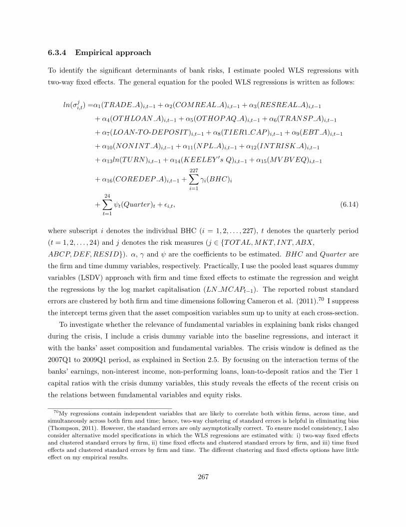
6.3.4 Empirical approach
To identify the significant determinants of bank risks, I estimate pooled WLS regressions with
two-way fixed effects. The general equation for the pooled WLS regressions is written as follows:
ln(σji,t) =α1(TRADE A)i,t−1 + α2(COMREAL A)i,t−1 + α3(RESREAL A)i,t−1
+ α4(OTHLOAN A)i,t−1 + α5(OTHOPAQ A)i,t−1 + α6(TRANSP A)i,t−1
+ α7(LOAN -TO-DEPOSIT )i,t−1 + α8(TIER1 CAP )i,t−1 + α9(EBT A)i,t−1
+ α10(NONINT A)i,t−1 + α11(NPL A)i,t−1 + α12(INTRISK A)i,t−1
+ α13ln(TURN)i,t−1 + α14(KEELEY′s Q)i,t−1 + α15(MVBV EQ)i,t−1
+ α16(COREDEP A)i,t−1 +
227∑i=1
γi(BHC)i
+
24∑t=1
ψt(Quarter)t + ϵi,t, (6.14)
where subscript i denotes the individual BHC (i = 1, 2, . . . , 227), t denotes the quarterly period
(t = 1, 2, . . . , 24) and j denotes the risk measures (j ∈ TOTAL,MKT, INT,ABX,
ABCP,DEF,RESID). α, γ and ψ are the coefficients to be estimated. BHC and Quarter are
the firm and time dummy variables, respectively. Practically, I use the pooled least squares dummy
variables (LSDV) approach with firm and time fixed effects to estimate the regression and weight
the regressions by the log market capitalisation (LN MCAPt−1). The reported robust standard
errors are clustered by both firm and time dimensions following Cameron et al. (2011).70 I suppress
the intercept terms given that the asset composition variables sum up to unity at each cross-section.
To investigate whether the relevance of fundamental variables in explaining bank risks changed
during the crisis, I include a crisis dummy variable into the baseline regressions, and interact it
with the banks’ asset composition and fundamental variables. The crisis window is defined as the
2007Q1 to 2009Q1 period, as explained in Section 2.5. By focusing on the interaction terms of the
banks’ earnings, non-interest income, non-performing loans, loan-to-deposit ratios and the Tier 1
capital ratios with the crisis dummy variables, this study reveals the effects of the recent crisis on
the relations between fundamental variables and equity risks.
70My regressions contain independent variables that are likely to correlate both within firms, across time, andsimultaneously across both firm and time; hence, two-way clustering of standard errors is helpful in eliminating bias(Thompson, 2011). However, the standard errors are only asymptotically correct. To ensure model consistency, I alsoconsider alternative model specifications in which the WLS regressions are estimated with: i) two-way fixed effectsand clustered standard errors by firm, ii) time fixed effects and clustered standard errors by firm, and iii) time fixedeffects and clustered standard errors by firm and time. The different clustering and fixed effects options have littleeffect on my empirical results.
267
6.4 Empirical results
6.4.1 Summary statistics
Table 6.2 reports the full sample and subsample means and standard deviations of the bank vari-
ables. First, the mean (median) of inflation-adjusted total bank assets is $51.7 ($1.5) billion. Loan
assets represent the largest proportion of bank assets averaging at 69.0% with 14.5% in commercial
real estate loans, 17.0% in residential real estate loans and 37.4% in other loans. Other opaque
assets, transparent assets and trade assets average at 23.7%, 6.4% and 0.7%, respectively. In com-
parison to Jones et al.’s (2013) study based on the 2000 to 2006 period, profound changes in the
banks’ loan asset composition are observed. In particular, banks have noticeably less commercial
real estate loan assets on their balance sheets, from 27.6% over 2000 to 2006 (as shown in Table
1 of Jones et al. (2013)) to my full sample mean values of 14.5% over 2006 to 2011, as shown in
Panel B. Because of concern over the heightening risk of mortgage default, banks have shifted from
commercial real estate loans (pre-crisis level of 34.1% reduced to the crisis level of 19.8%) into other
loans.71 Total loans to assets have increased from the pre-crisis 68.6% to 71.6% during the crisis
while trading assets also increased from 0.6% to 0.9%.
For the banks’ profitability, the full sample mean (median) earnings to total assets is 0.1% (0.9%)
while that of the non-interest income to total assets is 1.2% (1.0%). The subsample statistics show
that banks’ mean earnings to total assets declined from the pre-crisis level of 1.6% to 0.1% during
the crisis and to -0.4% during the post-crisis subsample. In addition, banks’ credit risks heightened
during and after the crisis as evinced by the increases in banks’ non-performing loans to total assets
from the pre-crisis level of 0.4% to 1.2% during the crisis, and further to 2.9% in the post-crisis
subsample. For the banks’ funding ability, the mean loan-to-deposit ratio has increased from 1.42
to 1.50 while the Tier 1 capital ratio has declined from 11.5% to 10.8% in the crisis subsample
suggesting that banks on average faced a more constrained funding position and had less equity
capital as a buffer to liquidity shocks.
All bank equity risks increased remarkably during the crisis, as shown in the crisis subsample
statistics and remained at considerably high levels in the post-crisis subsample. The banks’ full
sample mean (quarterly equivalent) TOTAL risk is 28.46% while the RESID risk represents the
largest risk component with a mean value of 24.26%. The second largest component of equity risk
refers to the MKT risk with a mean value of 10.20%. The full sample mean INT, ABX, ABCP,
and DEF risks are 2.23%, 2.56%, 2.69% and 2.27%, respectively.
71These statistics are consistent with Cornett et al. (2011) who show that during 2008, US commercial banksreceived more core deposits and extended more commercial and industrial (C&I) loans.
268
6.4.2 Determinants of bank equity risks - full sample
Table 6.3 reports the results of the baseline regressions of Equation 6.14 when either banks’ TOTAL,
MKT, INT, ABX, ABCP, DEF or RESID risks are the dependent variables. The model fit of the
WLS regressions is satisfactory and in general yield high R2 values: 81% (TOTAL), 65% (MKT),
31% (INT), 31% (ABX), 32% (ABCP), 30% (DEF) and 81% (RESID). F-tests of joint significance
on the right hand side variables for all six risk models are significant at the 1% significance level
and are not reported.
Regarding the banks’ asset composition, Hypothesis 1A is in general not supported in that
banks’ exposure to various types of loan assets does not explain bank equity risks. However, the
coefficients on all types of loan assets except the transparent assets are significant in explaining
the INT risks. Banks with more loan assets on their balance sheets were less impacted by the
variations in the 3-month Treasury bill rate, possibly because the banks’ ability to extend loans
during a period of high macroeconomic risk reflects the banks’ fundamental strength and relatively
stable sources of liquidity. Hypothesis 1B, which asserts that banks with more opaque assets are
more risky, is in general not supported. The F-tests of equality between the estimated parameters
of the five types of opaque assets and the transparent assets reveal that the impact of opaque
assets on bank equity risks are largely more negative than those of the transparent assets across all
risk models except the MKT and DEF risks (despite being insignificant). Banks’ investments in
relatively more opaque assets translate into lower bank equity risks somewhat consistent with Jones
et al. (2013) who conclude that the risks in banks’ opaque investments were not priced accurately.
I document compelling evidence that banks’ fundamental variables significantly determine the
seven bank equity risks, lending strong support to Hypotheses 2A, 3A, and 4A. First, the estimated
parameters of the banks’ earnings to total assets are statistically significant and negative in the
TOTAL, MKT, ABX, ABCP and RESID risk models. A one standard deviation increase in banks’
earnings to total assets (3.0%) would reduce (in logarithmic) TOTAL risk by 1.25%, MKT risk by
1.44%, ABX risk by 8.65%, ABCP risk by 5.88%, and RESID risk by 1.29%, approximately.72 The
statistically significant negative relation between the banks’ earnings and equity risks is informative
from the perspective of an investor and of a bank regulator in that banks with lower profitability
were more susceptible to the idiosyncratic shocks from the troubled structured finance market
and the asset-backed money market. In addition, the coefficients of banks’ non-interest income
to total assets are also significant in the TOTAL and RESID risk models so that banks with
more income arising from off-balance sheet activities and fee-based income (i.e. more diversified
sources of income) have less total and idiosyncratic risks. With regard to banks’ credit risks, as
72For instance, a one standard deviation increase in earnings to total assets (3.0%) would translate into [0.030 ∗−1.392
ln(28.458)= −0.0125] 1.25% lower TOTAL risks.
269
hypothesised in Hypothesis 3A, the coefficients on the non-performing loans to total assets are
highly significant and negative in the TOTAL, INT, ABX, DEF and RESID risk models. As for
the economic significance, a one standard deviation increase in banks’ non-performing loans to total
assets (2.1%) would increase TOTAL risk by 4.04%, INT risk by 35.90%, ABX risk by 14.80%,
DEF risk by 17.08%, and RESID risk by 5.05%, approximately. The evidence suggests that banks’
loan portfolio credit quality significantly determines bank equity risks and are negatively associated
with banks’ exposure to the variations in the 3-month Treasury bills, ABX AAA innovations and
market wide default risk. Likewise, the estimated parameters of the banks’ Tier 1 capital ratios are
highly significant and negative across all bank equity risks except the MKT risk, lending empirical
support for Hypothesis 2A. A one standard deviation increase in banks’ Tier 1 capital ratios (3.4%)
leads to 3.44% lower TOTAL risk, 26.18% lower INT risk, 13.01% lower ABX risk, 25.41% lower
ABCP risk, 22.18% lower DEF risk, and 3.99% lower RESID risk, approximately.
The evidence presented suggests that the market-based bank equity risks are related significantly
to banks’ sources of fundamental risks pertaining to profitability, loan portfolio credit quality and
capital adequacy. I am the first paper to unravel the within-bank relations between banks’ funda-
mental performance and equity risks and show empirically that banks with weaker fundamentals
were, to a larger extent, negatively affected by the crisis-related shocks originating from the trou-
bled structured finance market and related to the market wide default risk. The findings provide
useful implications to investment management and highlight the relevance of fundamental analysis
in evaluating bank stock performance during a period characterised by heightening macroeconomic
risk and uncertainty. From a supervisory perspective, my analysis documents the relationship be-
tween banks’ capital adequacy and equity risks, and (more importantly) demonstrates that banks
with higher levels of equity capital are less affected by systematic funding illiquidity shocks as
measured by the unexpected tightening in the ABCP spreads. The evidence presented leads us to
conclude that proper management in the banks’ regulatory capital requirement poses as an effective
preventive measure against systemic failure in relation to funding illiquidity.
6.4.3 Crisis interaction effects
Table 6.4 reports the results of my crisis models, with the crisis dummy and interaction variables.
The asset composition variables, earnings to total assets, non-interest income to total assets, non-
performing loans, loan-to-deposit ratios and the Tier 1 capital ratios are interacted with the crisis
dummy variables to allow for shift changes in the slope coefficients. Similarly, I report the results
of each crisis model when either the TOTAL, MKT, INT, ABX, ABCP, DEF, and RESID risks are
the dependent variables.
First, the coefficients of the crisis dummy variables are significant and positive in the TOTAL,
270
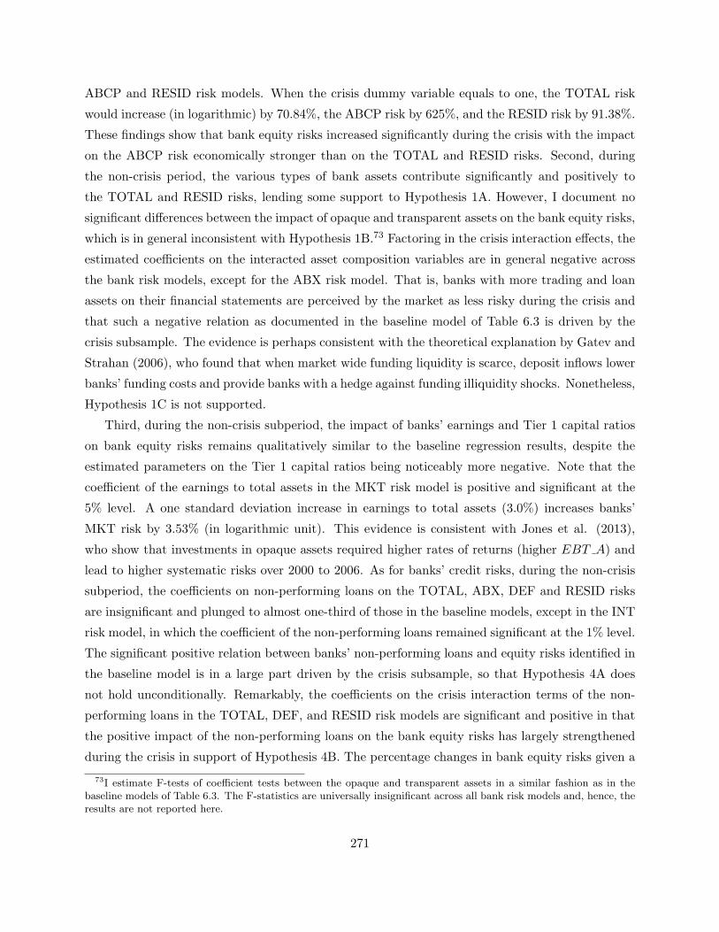
ABCP and RESID risk models. When the crisis dummy variable equals to one, the TOTAL risk
would increase (in logarithmic) by 70.84%, the ABCP risk by 625%, and the RESID risk by 91.38%.
These findings show that bank equity risks increased significantly during the crisis with the impact
on the ABCP risk economically stronger than on the TOTAL and RESID risks. Second, during
the non-crisis period, the various types of bank assets contribute significantly and positively to
the TOTAL and RESID risks, lending some support to Hypothesis 1A. However, I document no
significant differences between the impact of opaque and transparent assets on the bank equity risks,
which is in general inconsistent with Hypothesis 1B.73 Factoring in the crisis interaction effects, the
estimated coefficients on the interacted asset composition variables are in general negative across
the bank risk models, except for the ABX risk model. That is, banks with more trading and loan
assets on their financial statements are perceived by the market as less risky during the crisis and
that such a negative relation as documented in the baseline model of Table 6.3 is driven by the
crisis subsample. The evidence is perhaps consistent with the theoretical explanation by Gatev and
Strahan (2006), who found that when market wide funding liquidity is scarce, deposit inflows lower
banks’ funding costs and provide banks with a hedge against funding illiquidity shocks. Nonetheless,
Hypothesis 1C is not supported.
Third, during the non-crisis subperiod, the impact of banks’ earnings and Tier 1 capital ratios
on bank equity risks remains qualitatively similar to the baseline regression results, despite the
estimated parameters on the Tier 1 capital ratios being noticeably more negative. Note that the
coefficient of the earnings to total assets in the MKT risk model is positive and significant at the
5% level. A one standard deviation increase in earnings to total assets (3.0%) increases banks’
MKT risk by 3.53% (in logarithmic unit). This evidence is consistent with Jones et al. (2013),
who show that investments in opaque assets required higher rates of returns (higher EBT A) and
lead to higher systematic risks over 2000 to 2006. As for banks’ credit risks, during the non-crisis
subperiod, the coefficients on non-performing loans on the TOTAL, ABX, DEF and RESID risks
are insignificant and plunged to almost one-third of those in the baseline models, except in the INT
risk model, in which the coefficient of the non-performing loans remained significant at the 1% level.
The significant positive relation between banks’ non-performing loans and equity risks identified in
the baseline model is in a large part driven by the crisis subsample, so that Hypothesis 4A does
not hold unconditionally. Remarkably, the coefficients on the crisis interaction terms of the non-
performing loans in the TOTAL, DEF, and RESID risk models are significant and positive in that
the positive impact of the non-performing loans on the bank equity risks has largely strengthened
during the crisis in support of Hypothesis 4B. The percentage changes in bank equity risks given a
73I estimate F-tests of coefficient tests between the opaque and transparent assets in a similar fashion as in thebaseline models of Table 6.3. The F-statistics are universally insignificant across all bank risk models and, hence, theresults are not reported here.
271
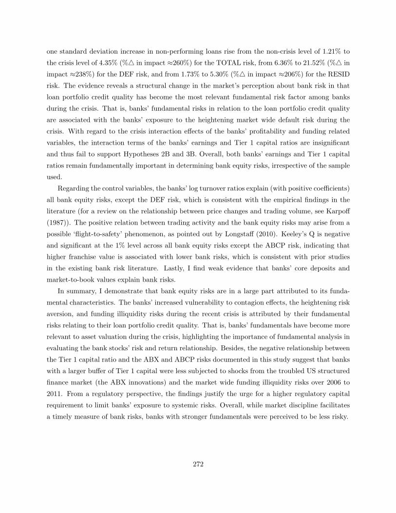
one standard deviation increase in non-performing loans rise from the non-crisis level of 1.21% to
the crisis level of 4.35% (% in impact ≈260%) for the TOTAL risk, from 6.36% to 21.52% (% in
impact ≈238%) for the DEF risk, and from 1.73% to 5.30% (% in impact ≈206%) for the RESID
risk. The evidence reveals a structural change in the market’s perception about bank risk in that
loan portfolio credit quality has become the most relevant fundamental risk factor among banks
during the crisis. That is, banks’ fundamental risks in relation to the loan portfolio credit quality
are associated with the banks’ exposure to the heightening market wide default risk during the
crisis. With regard to the crisis interaction effects of the banks’ profitability and funding related
variables, the interaction terms of the banks’ earnings and Tier 1 capital ratios are insignificant
and thus fail to support Hypotheses 2B and 3B. Overall, both banks’ earnings and Tier 1 capital
ratios remain fundamentally important in determining bank equity risks, irrespective of the sample
used.
Regarding the control variables, the banks’ log turnover ratios explain (with positive coefficients)
all bank equity risks, except the DEF risk, which is consistent with the empirical findings in the
literature (for a review on the relationship between price changes and trading volume, see Karpoff
(1987)). The positive relation between trading activity and the bank equity risks may arise from a
possible ‘flight-to-safety’ phenomenon, as pointed out by Longstaff (2010). Keeley’s Q is negative
and significant at the 1% level across all bank equity risks except the ABCP risk, indicating that
higher franchise value is associated with lower bank risks, which is consistent with prior studies
in the existing bank risk literature. Lastly, I find weak evidence that banks’ core deposits and
market-to-book values explain bank risks.
In summary, I demonstrate that bank equity risks are in a large part attributed to its funda-
mental characteristics. The banks’ increased vulnerability to contagion effects, the heightening risk
aversion, and funding illiquidity risks during the recent crisis is attributed by their fundamental
risks relating to their loan portfolio credit quality. That is, banks’ fundamentals have become more
relevant to asset valuation during the crisis, highlighting the importance of fundamental analysis in
evaluating the bank stocks’ risk and return relationship. Besides, the negative relationship between
the Tier 1 capital ratio and the ABX and ABCP risks documented in this study suggest that banks
with a larger buffer of Tier 1 capital were less subjected to shocks from the troubled US structured
finance market (the ABX innovations) and the market wide funding illiquidity risks over 2006 to
2011. From a regulatory perspective, the findings justify the urge for a higher regulatory capital
requirement to limit banks’ exposure to systemic risks. Overall, while market discipline facilitates
a timely measure of bank risks, banks with stronger fundamentals were perceived to be less risky.
272
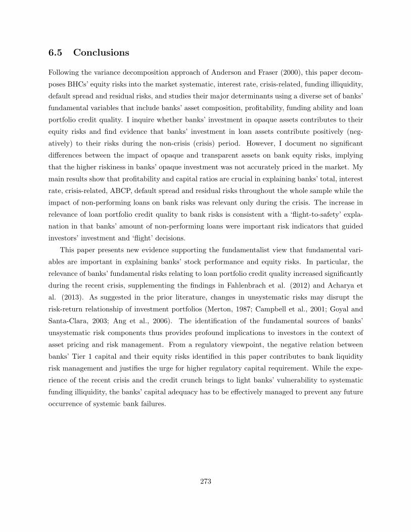
6.5 Conclusions
Following the variance decomposition approach of Anderson and Fraser (2000), this paper decom-
poses BHCs’ equity risks into the market systematic, interest rate, crisis-related, funding illiquidity,
default spread and residual risks, and studies their major determinants using a diverse set of banks’
fundamental variables that include banks’ asset composition, profitability, funding ability and loan
portfolio credit quality. I inquire whether banks’ investment in opaque assets contributes to their
equity risks and find evidence that banks’ investment in loan assets contribute positively (neg-
atively) to their risks during the non-crisis (crisis) period. However, I document no significant
differences between the impact of opaque and transparent assets on bank equity risks, implying
that the higher riskiness in banks’ opaque investment was not accurately priced in the market. My
main results show that profitability and capital ratios are crucial in explaining banks’ total, interest
rate, crisis-related, ABCP, default spread and residual risks throughout the whole sample while the
impact of non-performing loans on bank risks was relevant only during the crisis. The increase in
relevance of loan portfolio credit quality to bank risks is consistent with a ‘flight-to-safety’ expla-
nation in that banks’ amount of non-performing loans were important risk indicators that guided
investors’ investment and ‘flight’ decisions.
This paper presents new evidence supporting the fundamentalist view that fundamental vari-
ables are important in explaining banks’ stock performance and equity risks. In particular, the
relevance of banks’ fundamental risks relating to loan portfolio credit quality increased significantly
during the recent crisis, supplementing the findings in Fahlenbrach et al. (2012) and Acharya et
al. (2013). As suggested in the prior literature, changes in unsystematic risks may disrupt the
risk-return relationship of investment portfolios (Merton, 1987; Campbell et al., 2001; Goyal and
Santa-Clara, 2003; Ang et al., 2006). The identification of the fundamental sources of banks’
unsystematic risk components thus provides profound implications to investors in the context of
asset pricing and risk management. From a regulatory viewpoint, the negative relation between
banks’ Tier 1 capital and their equity risks identified in this paper contributes to bank liquidity
risk management and justifies the urge for higher regulatory capital requirement. While the expe-
rience of the recent crisis and the credit crunch brings to light banks’ vulnerability to systematic
funding illiquidity, the banks’ capital adequacy has to be effectively managed to prevent any future
occurrence of systemic bank failures.
273

Table 6.1: Variables descriptionThis table contains a description of the bank variables used in this study. All accounting variables are computed as averagesof beginning and ending quarter values, deflated using a seasonally adjusted GDP deflator with a base year of 2005.
Variables Description
Panel A: Asset composition variables
TRADE A Trading assets to total assets.
LOAN A Total loans to total assets.
COMREAL A Commercial real estate loans to total assets.
RESREAL A Residential real estate loans to total assets.
OTHLOAN A All other loans to total assets.
OTHOPAQ A All other opaque assets to total assets. All other opaque assets includeavailable-for-sale or held-to-maturity MBS or ABS that are not guaranteed bya government entity, fixed assets, investments in unconsolidated subsidiariesand other real estate investments.
TRANSP A All transparent assets to total assets. All transparent assets include cash,federal funds sold, securities under reselling agreement, guaranteed available-for-sale and held-to-maturity securities.
Note: TRADE A+ COMREAL A+RESREAL A+OTHLOAN A+OTHOPAQ A+ TRANSP A = 1.
Panel B: Bank profitability
EBT A The earnings before extraordinary items and taxes normalised by total assets(annualised).
NONINT A Non-interest income to total assets (annualised).
Panel C: Bank fundamental risks
NPL A Proportion of non-performing loans to total assets as a measure of credit risks.
Panel D: Bank funding variables
LOAN -TO-DEPOSIT Ratio of total loans to core deposits.
TIER1 CAP Tier 1 risk-based capital ratio (BHCK7206).
Panel E: Market variables
LN TURN Log turnover ratios. Turnover ratio is the number of traded shares overthe number of outstanding shares in a month. The ratio I use is the logtransform of the monthly average of turnover ratios over the three months ineach quarter.
Panel F: Other variables
INTRISK A The absolute value of the difference between short-term assets and short-term liabilities and equity, normalised by total asset, as a measure of banks’exposure to interest rate risk.
KEELEY ′s Q The sum of market value of common equity and the book value of liabilitiesdivided by the book value of assets. It is used as a measure of franchise value(see, Anderson and Fraser, 2000).
MVBV EQ The ratio of market value to book value of equity.
COREDEP A The amount of core deposit scaled by the total assets.
MCAP The market capitalisation of a bank stock, computed as the product of itsprice and number of shares outstanding at the end of each quarter.
BV EQ The book value of the total shareholders’ equity of a banking firm.
274
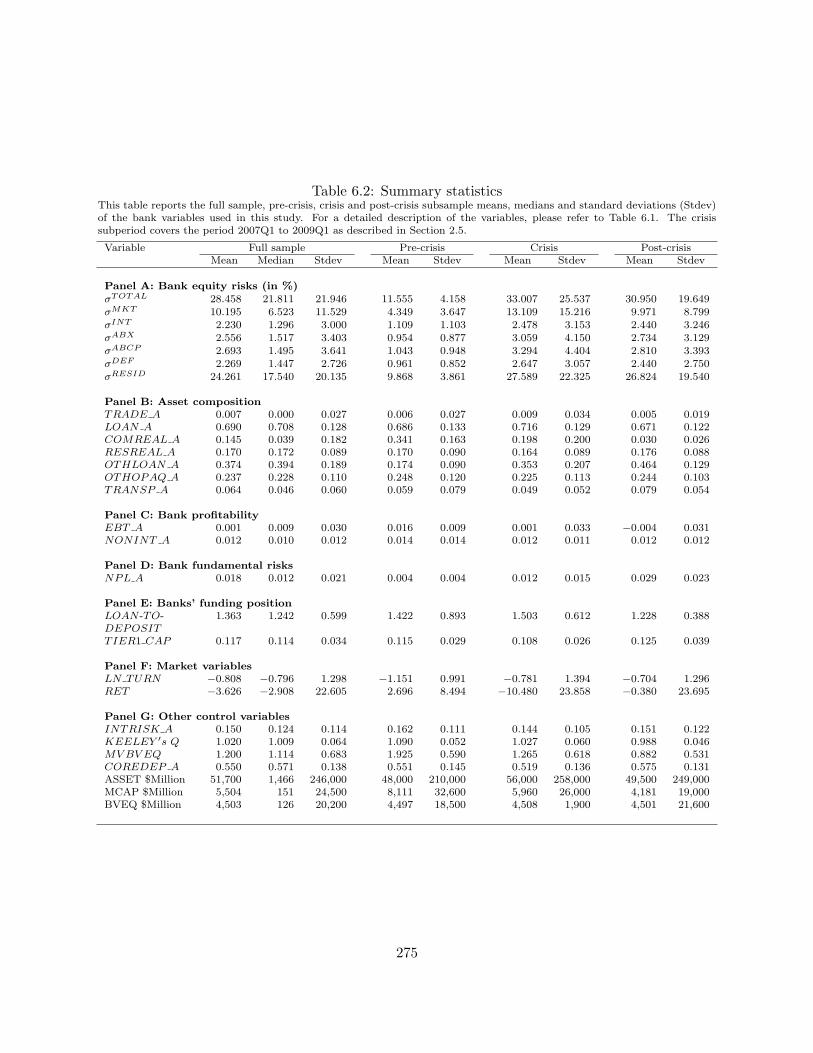
Table 6.2: Summary statisticsThis table reports the full sample, pre-crisis, crisis and post-crisis subsample means, medians and standard deviations (Stdev)of the bank variables used in this study. For a detailed description of the variables, please refer to Table 6.1. The crisissubperiod covers the period 2007Q1 to 2009Q1 as described in Section 2.5.
Variable Full sample Pre-crisis Crisis Post-crisisMean Median Stdev Mean Stdev Mean Stdev Mean Stdev
Panel A: Bank equity risks (in %)σTOTAL 28.458 21.811 21.946 11.555 4.158 33.007 25.537 30.950 19.649σMKT 10.195 6.523 11.529 4.349 3.647 13.109 15.216 9.971 8.799σINT 2.230 1.296 3.000 1.109 1.103 2.478 3.153 2.440 3.246σABX 2.556 1.517 3.403 0.954 0.877 3.059 4.150 2.734 3.129σABCP 2.693 1.495 3.641 1.043 0.948 3.294 4.404 2.810 3.393σDEF 2.269 1.447 2.726 0.961 0.852 2.647 3.057 2.440 2.750σRESID 24.261 17.540 20.135 9.868 3.861 27.589 22.325 26.824 19.540
Panel B: Asset compositionTRADE A 0.007 0.000 0.027 0.006 0.027 0.009 0.034 0.005 0.019LOAN A 0.690 0.708 0.128 0.686 0.133 0.716 0.129 0.671 0.122COMREAL A 0.145 0.039 0.182 0.341 0.163 0.198 0.200 0.030 0.026RESREAL A 0.170 0.172 0.089 0.170 0.090 0.164 0.089 0.176 0.088OTHLOAN A 0.374 0.394 0.189 0.174 0.090 0.353 0.207 0.464 0.129OTHOPAQ A 0.237 0.228 0.110 0.248 0.120 0.225 0.113 0.244 0.103TRANSP A 0.064 0.046 0.060 0.059 0.079 0.049 0.052 0.079 0.054
Panel C: Bank profitabilityEBT A 0.001 0.009 0.030 0.016 0.009 0.001 0.033 −0.004 0.031NONINT A 0.012 0.010 0.012 0.014 0.014 0.012 0.011 0.012 0.012
Panel D: Bank fundamental risksNPL A 0.018 0.012 0.021 0.004 0.004 0.012 0.015 0.029 0.023
Panel E: Banks’ funding positionLOAN -TO-DEPOSIT
1.363 1.242 0.599 1.422 0.893 1.503 0.612 1.228 0.388
TIER1 CAP 0.117 0.114 0.034 0.115 0.029 0.108 0.026 0.125 0.039
Panel F: Market variablesLN TURN −0.808 −0.796 1.298 −1.151 0.991 −0.781 1.394 −0.704 1.296RET −3.626 −2.908 22.605 2.696 8.494 −10.480 23.858 −0.380 23.695
Panel G: Other control variablesINTRISK A 0.150 0.124 0.114 0.162 0.111 0.144 0.105 0.151 0.122KEELEY ′s Q 1.020 1.009 0.064 1.090 0.052 1.027 0.060 0.988 0.046MVBV EQ 1.200 1.114 0.683 1.925 0.590 1.265 0.618 0.882 0.531COREDEP A 0.550 0.571 0.138 0.551 0.145 0.519 0.136 0.575 0.131ASSET $Million 51,700 1,466 246,000 48,000 210,000 56,000 258,000 49,500 249,000MCAP $Million 5,504 151 24,500 8,111 32,600 5,960 26,000 4,181 19,000BVEQ $Million 4,503 126 20,200 4,497 18,500 4,508 1,900 4,501 21,600
275
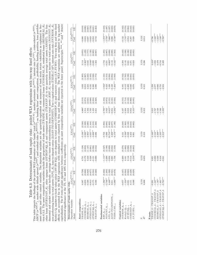
Tab
le6.3:
Determinan
tsofbankequityrisks-pooledW
LSregressionswithtw
o-w
ayfixed
effects
This
table
reportsth
efindingsofth
epooledW
LSregressionsofth
ebanks’
total(σ
TOTAL),
market
system
atic(σ
MK
T),
interest
rate
(σIN
T),
crisis-related(σ
ABX),
ABCP
(σABCP),
market
widedefault
spread(σ
DEF)andresidualrisks(σ
RESID)onbankingfirm
s’asset
composition,profitability,
fundingposition,loanportfolio
asset
quality
and
oth
erco
ntrolvariables.
Thedep
enden
tvariablesare
thequarterly-equivalentrisk
mea
suresofbankstock
retu
rnvolatilities
asex
plained
inSec-
tion6.3.2.Theasset
compositionvariablesincludeth
eproportionoftradeassets(T
RADE
A),
commercialloans(C
OM
REAL
A),
residen
tialloans(R
ESREAL
A),
oth
erloans(O
THLOAN
A),
oth
eropaqueloans(O
THOPAQ
A)andtransp
arentassets(T
RANSP
A)to
thequarterly
averagetotalassets(A
SSET).
Thefun-
damen
talandmarket
variablesinclude:
earn
ingsbefore
taxes
andex
traord
inary
item
sto
totalassets(E
BT
A),
non-interest
inco
meto
totalassets(N
ONINT
A),
non-perform
ingloansto
totalassets(N
PL
A),
loan-to-dep
ositratios(L
OAN-T
O-D
EPOSIT),
Tier1ca
pitalratios(T
IER1CAP),
interest
rate
risk
(INTRISK
A),
Keeley’s
Q,market-to-bookvalueratios(M
VBVEQ),
core
dep
osits
tototalassets(C
OREDEP
A)andtu
rnover
ratios(L
NTURN).
Two-w
ayfirm
andtimefixed
effects
are
accounted
forin
theW
LS
regressionswith
standard
errors
clustered
by
firm
and
timedim
ensions.
TheW
LS
regressionsare
weighted
by
logmarket
capitalisation.TheF-tests
ofjointsignifica
nce
betweenco
efficien
tsonasset
compositionvariablesare
reported
inth
elower
panel.Superscripts
***,**and*den
ote
statisticalsignifica
nce
atth
e1%,5%
and10%
level,resp
ectively.
Dete
rm
inants
ofbank
equity
risks
Dep
enden
tVariables
LN(σ
TOTAL
t)
LN(σ
MK
Tt
)LN(σ
IN
Tt
)LN(σ
ABX
t)
LN(σ
ABCP
t)
LN(σ
DEF
t)
LN(σ
RESID
t)
Model
Coef.
S.E
.Coef.
S.E
.Coef.
S.E
.Coef.
S.E
.Coef.
S.E
.Coef.
S.E
.Coef.
S.E
.
Assetcom
position:
TRADE
At−
10.387
(0.729)
0.731
(1.128)
−5.136∗∗
(2.530)
4.866∗
(2.513)
1.632
(2.305)
3.114
(2.655)
−0.080
(0.818)
COM
REAL
At−
1−0.659
(0.666)
−0.179
(0.959)
−2.820∗∗
(1.339)
1.514
(2.074)
0.013
(1.967)
−2.362∗∗
(1.109)
−0.624
(0.696)
RESREAL
At−
1−0.599
(0.829)
0.440
(1.147)
−2.905∗
(1.680)
1.102
(2.041)
2.224
(2.225)
−0.825
(1.777)
−0.607
(0.867)
OTHLOAN
At−
1−0.813
(0.677)
0.326
(0.981)
−4.031∗∗
∗(1.444)
1.705
(2.088)
0.135
(2.105)
−2.048∗
(1.120)
−0.823
(0.733)
OTHOPAQ
At−
1−0.175
(0.584)
−0.131
(0.598)
−3.008∗∗
(1.218)
1.416
(2.224)
0.386
(1.920)
−0.895
(0.905)
−0.052
(0.621)
TRANSP
At−
10.588
(0.460)
−0.090
(0.552)
−0.696
(1.300)
3.251
(2.368)
2.890
(1.774)
−1.304
(0.987)
0.716
(0.464)
Fundam
enta
lvariables:
EBT
At−
1−1.392∗∗
∗(0.402)
−1.113∗∗
(0.527)
−0.733
(1.094)
−2.705∗∗
(1.194)
−1.943∗
(1.131)
−1.716
(1.455)
−1.372∗∗
∗(0.418)
NONINT
At−
1−2.746∗∗
(1.204)
−3.200
(2.196)
−4.690
(3.684)
1.043
(4.872)
0.423
(4.154)
−0.551
(2.987)
−2.750∗
(1.497)
NPL
At−
16.449∗∗
∗(1.320)
−3.934
(2.839)
13.710∗∗
∗(2.462)
6.615∗∗
(3.151)
1.438
(2.956)
6.663∗∗
(2.608)
7.666∗∗
∗(1.327)
LOAN-T
O-D
EPOSITt−
10.011
(0.021)
0.005
(0.032)
0.208∗∗
∗(0.077)
−0.054
(0.135)
−0.108
(0.094)
−0.116
(0.080)
0.006
(0.023)
TIER1CAPt−
1−3.386∗∗
∗(0.676)
−1.756
(1.559)
−6.176∗∗
∗(1.196)
−3.592∗∗
(1.656)
−7.404∗∗
∗(1.910)
−5.345∗∗
∗(1.563)
−3.738∗∗
∗(0.678)
Controlvariables:
INTRISK
At−
1−0.077
(0.167)
−0.269
(0.278)
0.131
(0.349)
0.437
(0.515)
0.105
(0.542)
−0.394
(0.443)
−0.132
(0.162)
Keeley′ s
Qt−
1−1.316∗∗
(0.564)
0.161
(1.063)
−2.336∗
(1.363)
−2.504
(1.714)
−0.112
(1.765)
−2.145
(1.330)
−1.745∗∗
∗(0.570)
MVBVEQ
t−1
−0.031
(0.063)
0.144
(0.096)
−0.028
(0.146)
0.018
(0.122)
−0.209
(0.190)
0.021
(0.106)
−0.054
(0.064)
COREDEP
At−
10.171
(0.238)
−0.514
(0.534)
0.252
(0.644)
0.053
(0.866)
−0.826
(0.681)
0.271
(0.603)
0.287
(0.242)
LN
TURN
t−1
0.046
(0.029)
0.216∗∗
∗(0.063)
0.061
(0.062)
0.155∗∗
∗(0.045)
0.070
(0.055)
−0.024
(0.055)
0.028
(0.025)
N3,153
3,153
3,153
3,153
3,153
3,153
3,153
R2
0.806
0.653
0.310
0.312
0.315
0.296
0.814
F-tests
TRADE
A−
TRANSP
A−0.201
0.821
−4.440∗∗
1.615
−1.258
4.418∗
−0.796
COM
REAL
A−
TRANSP
A−1.247∗∗
∗−0.089
−2.124∗∗
−1.737
−2.877
−1.058
−1.340∗∗
∗
RESREAL
A−
TRANSP
A−1.187∗
0.530
−2.209∗∗
−2.149
−0.666
0.479
−1.323∗∗
OTHLOAN
A−
TRANSP
A−1.401∗∗
∗0.416
−3.335∗∗
∗−1.546
−2.755
−0.744
−1.539∗∗
∗
OTHOPAQ
A−
TRANSP
A−0.763∗∗
∗−0.041
−2.312∗∗
∗−1.835∗∗
−2.504
0.409
−0.768∗∗
276

Tab
le6.4:
Determinan
tsof
ban
kequityriskswithcrisis
dummyandinteractions-pooledW
LSregressionswithtw
o-way
fixed
effects
This
table
reportsth
efindingsofth
epooledW
LSregressionsofth
ebanks’
total(σ
TOTAL),
market
system
atic(σ
MK
T),
interest
rate
(σIN
T),
crisis-related(σ
ABX),
ABCP
(σABCP),
market
widedefault
spread(σ
DEF)andresidualrisks(σ
RESID)onbankingfirm
s’asset
composition,profitability,
fundingposition,loanportfolio
asset
quality
and
oth
erco
ntrolvariables.
To
captu
reth
ecrisis
effect,
Iincludea
crisis
dummy
variable
(crisisperiod:
2007Q1-2009Q1)and
interact
thecrisis
dummyvariable
withth
ebankingfirm
s’fundamen
talvariablesandasset
compositionvariables.
Thedep
enden
tvariablesare
thequarterly-equivalentrisk
mea
sures
ofbankstock
retu
rnvolatilities
asex
plained
inSection6.3.2.Theasset
compositionvariablesincludeth
eproportionoftradeassets(T
RADE
A),
commercialloans
(COM
REAL
A),
residen
tialloans(R
ESREAL
A),
oth
erloans(O
THLOAN
A),
oth
eropaqueloans(O
THOPAQ
A)andtransp
arentassets(T
RANSP
A)to
the
quarterly
averagetotalassets(A
SSET).
Thefundamen
taland
market
variablesinclude:
earn
ingsbefore
taxes
and
extraord
inary
item
sto
totalassets(E
BT
A),
non-interest
inco
meto
totalassets(N
ONINT
A),non-perform
ingloansto
totalassets(N
PL
A),loan-to-dep
ositratios(L
OAN-T
O-D
EPOSIT),Tier1ca
pitalratios
(TIER1CAP),
interest
rate
risk
(INTRISK
A),
Keeley’s
Q,market-to-bookvalueratios(M
VBVEQ),
core
dep
osits
tototalassets(C
OREDEP
A)andtu
rnover
ratios(L
NTURN).
Two-w
ayfirm
andtimefixed
effects
are
accountedforin
theW
LSregressionswithstandard
errors
clustered
byfirm
andtimedim
ensions.
The
WLSregressionsare
weightedbylogmarket
capitalisation.Superscripts
***,**and*den
ote
statisticalsignifica
nce
atth
e1%,5%
and10%
level,resp
ectively.
Dete
rm
inants
ofbank
equity
risks
Dep
enden
tVariables
LN(σ
TOTAL
t)
LN(σ
MK
Tt
)LN(σ
IN
Tt
)LN(σ
ABX
t)
LN(σ
ABCP
t)
LN(σ
DEF
t)
LN(σ
RESID
t)
Model
Coef.
S.E
.Coef.
S.E
.Coef.
S.E
.Coef.
S.E
.Coef.
S.E
.Coef.
S.E
.Coef.
S.E
.
Assetcom
position:
TRADE
At−
12.014
(1.263)
−0.179
(2.015)
3.344
(3.792)
3.154
(4.007)
6.044
(3.723)
4.112
(4.639)
2.798∗∗
(1.335)
COM
REAL
At−
11.120
(0.792)
−0.782
(1.746)
−2.462
(1.540)
3.269∗
(1.764)
3.334
(3.032)
−0.810
(1.553)
1.843∗∗
(0.766)
RESREAL
At−
10.448
(0.915)
−0.509
(1.657)
−2.316
(1.767)
1.293
(1.896)
3.989
(3.004)
0.121
(2.256)
1.277
(0.933)
OTHLOAN
At−
11.995∗∗
∗(0.744)
1.422
(1.557)
−1.577
(1.570)
3.537∗
(1.888)
4.505
(3.080)
−0.056
(1.652)
2.492∗∗
∗(0.755)
OTHOPAQ
At−
11.125∗
(0.587)
0.163
(0.885)
−1.918
(1.444)
1.388
(1.969)
3.325
(2.875)
−0.327
(1.596)
1.585∗∗
(0.644)
TRANSP
At−
11.610∗∗
(0.775)
0.211
(1.003)
−0.214
(1.756)
2.795
(2.232)
4.865∗
(2.799)
−0.860
(1.861)
1.917∗∗
(0.768)
Fundam
enta
lvariables:
EBT
At−
1−0.868
(0.719)
2.733∗∗
(1.303)
0.677
(1.263)
−2.004
(1.470)
−2.724∗
(1.450)
−2.828∗
(1.578)
−1.718∗∗
(0.705)
NONINT
At−
1−3.642
(2.247)
−7.215∗∗
(3.597)
−7.121∗
(4.012)
2.019
(5.947)
0.734
(4.699)
−0.418
(4.224)
−2.542
(2.090)
NPL
At−
11.937
(1.842)
−5.277
(3.437)
9.507∗∗
∗(2.829)
4.572
(2.849)
−4.198
(3.367)
2.480
(2.806)
2.624
(1.736)
LOAN-T
O-D
EPOSITt−
1−0.084∗∗
(0.039)
−0.109∗
(0.056)
0.113
(0.077)
−0.217
(0.182)
−0.186
(0.134)
−0.182∗∗
(0.086)
−0.082∗
(0.045)
TIER1CAPt−
1−3.796∗∗
∗(1.241)
−1.148
(2.175)
−5.958∗∗
∗(1.475)
−4.885∗∗
∗(1.543)
−8.000∗∗
∗(2.346)
−5.933∗∗
∗(1.472)
−4.693∗∗
∗(1.066)
Crisis
dum
my
and
inte
raction
variables
CRISISt
2.372∗∗
∗(0.913)
0.612
(1.400)
2.054
(1.688)
−0.232
(2.410)
5.868∗
(3.203)
1.604
(2.464)
2.914∗∗
∗(0.836)
CRISISt×
TRADE
At−
1−1.621
(1.050)
1.100
(1.239)
−7.299∗∗
∗(2.777)
2.021
(3.231)
−6.556∗
(3.667)
−0.782
(2.729)
−2.849∗∗
∗(0.982)
OTHLOAN
At−
1−2.020∗∗
(0.935)
−0.017
(1.471)
−1.130
(1.756)
0.332
(2.456)
−5.421∗
(3.170)
−1.616
(2.381)
−2.579∗∗
∗(0.840)
OTHOPAQ
At−
1−2.241∗∗
(0.970)
−0.816
(1.465)
−1.579
(1.720)
0.835
(2.927)
−5.682∗
(3.191)
−1.399
(2.338)
−2.777∗∗
∗(0.918)
TRANSP
At−
1−2.176∗∗
(1.014)
−1.048
(1.668)
−0.842
(1.731)
1.018
(3.255)
−3.532
(3.632)
−1.748
(2.431)
−2.515∗∗
∗(0.968)
COM
REAL
At−
1−2.823∗∗
∗(1.024)
−0.396
(1.566)
−1.928
(1.713)
−0.414
(2.574)
−6.764∗∗
(3.104)
−2.087
(2.277)
−3.408∗∗
∗(0.913)
RESREAL
At−
1−2.008∗∗
(0.972)
−0.362
(1.508)
−1.818
(1.600)
1.131
(2.520)
−4.396
(3.210)
−1.691
(2.096)
−2.611∗∗
∗(0.876)
EBT
At−
1−0.671
(1.147)
−5.534∗∗
∗(1.830)
−2.855
(1.999)
−1.593
(1.985)
1.822
(1.983)
1.077
(1.877)
0.392
(1.035)
NONINT
At−
12.658
(2.561)
8.093∗∗
(3.697)
1.527
(5.473)
3.050
(7.188)
−3.900
(4.912)
−0.014
(6.144)
0.717
(2.378)
NPL
At−
15.005∗∗
(2.114)
1.130
(4.289)
−2.049
(3.710)
3.918
(2.770)
1.868
(4.361)
5.918∗
(3.374)
5.424∗∗
∗(2.041)
LOAN-T
O-D
EPOSITt−
1−0.065
(0.044)
0.004
(0.075)
−0.090
(0.103)
0.095
(0.114)
−0.140
(0.105)
−0.053
(0.098)
−0.089∗
(0.047)
TIER1CAPt−
10.025
(0.016)
0.015
(0.029)
0.009
(0.030)
0.004
(0.035)
0.022
(0.041)
0.041
(0.031)
0.029∗∗
(0.013)
Controlvariables:
INTRISK
At−
10.275
(0.232)
0.236
(0.315)
0.597
(0.443)
0.718
(0.593)
0.500
(0.576)
−0.303
(0.479)
0.154
(0.226)
Keeley′ s
Qt−
1−4.138∗∗
∗(1.056)
−2.888∗
(1.539)
−4.821∗∗
∗(1.475)
−6.448∗∗
∗(1.724)
−2.224
(1.770)
−4.278∗∗
∗(1.348)
−4.511∗∗
∗(0.948)
MVBVEQ
t−1
−0.020
(0.082)
0.126
(0.119)
0.042
(0.159)
0.034
(0.141)
−0.241
(0.200)
0.024
(0.122)
−0.026
(0.082)
COREDEP
At−
1−0.493
(0.529)
−0.508
(0.913)
−0.323
(0.563)
−0.816
(0.974)
−1.305
(0.842)
−0.429
(0.630)
−0.692
(0.443)
LN
TURN
t−1
0.138∗∗
∗(0.044)
0.326∗∗
∗(0.062)
0.143∗∗
(0.071)
0.237∗∗
∗(0.054)
0.169∗
(0.092)
0.060
(0.054)
0.112∗∗
∗(0.041)
N3,153
3,153
3,153
3,153
3,153
3,153
3,153
R2
0.669
0.576
0.267
0.282
0.270
0.259
0.721
277

THIS PAGE INTENTIONALLY LEFT BLANK
278
Chapter 7
The Predictability of Bank Stock
Returns and Its Implications for the
Asset ‘Fire Sales’ and
‘Flight-to-Safety’ Phenomena
7.1 Introduction
In the literature, there is ample evidence that BHCs’ stock returns can be predicted by a number of
fundamental variables (see Cooper et al., 2003; Bessler et al., 2007). Recent evidence suggests that
predictability in bank returns might have existed during the recent 2007 to 2009 financial crisis.
Fahlenbrach et al. (2012) compare bank stock performance across the 1998 and recent 2007 to
2009 financial crises and show that the banks’ exposure to illiquid assets and leverage contribute
positively to their under-performance. Acharya et al. (2013) study the banks’ securitisation and
the issuance of ABCPs, and document a similar conclusion that banks with higher exposure to the
ABCP conduits under-performed during the recent crisis. This evidence supports the fundamental-
ist viewpoint that fundamental variables are relevant in explaining bank stock returns. Motivated
by these research, this study updates the bank return predictability literature and formulates an
out-of-sample setting to test whether fundamental variables predict one-quarter ahead bank stock
returns, based on a sample period that covers the recent 2007 to 2009 financial crisis and part of
the ongoing European sovereign debt crisis. My main contributions to the literature are threefold.
First, this study focuses on the identification of the determinants of one-quarter ahead bank stock
returns over a sample period characterised by increasing risk aversion and volatilities. I demonstrate
how the banking firm’s characteristics reflect their fundamental risks during the crisis and highlight
the relevance of fundamental analysis in evaluating bank stock performance, providing profound
279
implications to a wide range of market users (including the retail and institutional investors, etc.)
in the context of investment and risk management. Second, to my knowledge, this study is the first
to document solid evidence that the bank’s fundamental variables significantly predicted future
trading activities in bank stocks, both during and after the crisis. My analysis uses both trading
ratio and order flow measures to gauge the intensity and direction of trading. The evidence that
banks with weaker fundamentals and of a smaller size were traded more intensely during the crisis
and that the higher trading activity was dominated by sell pressure leads me to conclude that
the bank stock return predictability pertains to investors’ asset ‘fire sale’ and ‘flight-to-safety’ be-
haviour during the crisis. In other words, the bank’s fundamentals and size were the major criteria
evaluated by investors in formulating their ‘flight’ decision. Third, I propose and demonstrate how
the banking firm’s fundamental variables can guide profitable investable strategies, both during
and after a crisis.
A number of previous studies have documented evidence of a ‘fire sale’ and of a ‘flight-to-safety’
from financial stocks during the recent 2007 to 2009 financial crisis. A ‘fire sale’ of an asset is
described as a forced sale, usually at prices far below intrinsic values, that can arise for various
reasons, for example: deleveraging and fund redemption requirements among hedge funds (Ben-
David et al., 2012), investors’ ‘flight’ to funds domiciled in developed markets (Jotikasthira et
al., 2012), capital withdrawals by mutual fund shareholders (Coval and Stafford, 2007), and the
commercial bank’s funding obligations after huge losses (French et al., 2010, pp. 67), etc. Anand
et al. (2013) show that buy-side institutions avoided trading illiquid stocks during the recent crisis
while Longstaff (2010) notes that the financial stocks were traded more intensely during the crisis,
which is consistent with portfolio rebalancing for risk management purposes and possible ‘flight-
to-safety’ into safer and more liquid asset classes. Taken together, the phenomenon of ‘fire sales’
or ‘flight-to-safety’ from illiquid financial stocks may have a considerable impact on their returns
(Coval and Stafford, 2007) and may account for the possible return predictability among bank
stocks. I argue that the criteria by which investors base their ‘fire sale’ or ‘flight’ decisions pertain
to the bank’s fundamental variables. In other words, investors might have excessively sold bank
stocks with poor fundamentals, leading to a relation between past fundamental performance and
future stock returns during the recent crisis. In this study, I conjecture that those banking firms
with the worst fundamentals might be more subject to the asset ‘fire sales’ or the ‘flight-to-safety’
phenomena, and have consistently under-performed.
Following the prior literature of the bank’s fundamental variables, I consider include those
variables relating to the bank’s return volatilities (Anderson and Fraser, 2000; Ang et al., 2006,
2009), earnings (Basu, 1983; Cooper et al., 2003), loan portfolio credit quality (Thakor, 1987;
280
Wahlen, 1994; Meeker and Gray, 1997; Jones et al., 2013)74, exposure to funding illiquidity risks
(Fahlenbrach et al., 2012; Acharya et al., 2013), non-interest income (Cooper et al., 2003; Bessler
et al., 2007), size (Banz, 1981; Gandhi and Lustig, 2011) and turnover ratios (Chordia et al.,
2001). There are a couple of distinct features specific to this study, as follows. First, in the context
of the recent crisis, banking firms’ exposure to the structured finance market (measured by the
ABX AAA index, a benchmark index for the US structured finance market) may affect bank stock
returns, evidence of contagion from the structured finance market to the US financial stocks has
been documented (Longstaff, 2010). The banks’ exposure to the structured finance market may
stem from their holding of trade assets, which include the subprime related structured securities
(Jones et al., 2013), and this represents a considerable source of fundamental risks. To this end, a
component of return volatilities relating to the variations of the ABX AAA index (denoted hereafter
as the ABX risk) is considered, following the variance decomposition approach of Anderson and
Fraser (2000). The evidence in this study shows that the banks’ ABX risk possess significant
predictive power over future bank stock returns. Second, prior studies suggest that banking firms’
exposure to funding illiquidity risks has a considerable impact on bank stock returns during the
crisis (Fahlenbrach et al., 2012; Acharya et al., 2013). The main source of banks’ vulnerability
to funding illiquidity risks commonly points to the maturity mismatch feature in the ‘shadow’
banking system in which banks issue structured finance securities via off-balance sheet conduits
(Brunnermeier, 2009). These conduits issue short-term ABCP to fund their purchases of longer-
term structured finance securities; for example, ABSs, RMBSs and CDOs. Banking firms were
responsible for providing contingent funding to the conduits via credit line facilities and were,
therefore, subject to tremendous funding illiquidity risks during the crisis. Given the unique nature
of the banks’ off-balance sheet activities and liquidity risk relating to their credit line commitments,
to my knowledge, this is one of the first papers that empirically examines the relationship between
banking firms’ exposure to funding illiquidity risks and future stock returns within the context of
asset pricing.
To anticipate some of my findings, the banks’ earnings, non-performing loans, loan-to-deposit
ratios, Tier 1 capital ratios, bank size, idiosyncratic and ABX risks are univariately important in
explaining the cross-section of one-quarter ahead bank stock returns. Banking firms with lower
profitability, more non-performing loans, lower Tier 1 capital ratios, higher loan-to-deposit ratios,
smaller market capitalisation, higher idiosyncratic and ABX risks have significantly lower simple
and risk-adjusted returns in the next quarter. The multivariate analysis based on the Fama and
Macbeth (1973) and the fixed effects panel regressions confirm the importance of banks’ earnings,
74Jones et al. (2013) find that non-performing loans to total assets is negatively related to excess market equityvalue above book value while Meeker and Gray (1997) show that the amount of non-performing loans are a satisfactorymeasure of bank asset quality.
281

non-performing loans, ABX risk and Tier 1 capital ratios in determining the one-quarter ahead
bank stock returns. Since a size effect is prominent, I conduct a two-way sort portfolio analysis to
disentangle the size effect from the predictability of other bank variables. I find that the predictive
power of the banks’ fundamental variables is evident within the small (0-30%) and mid (31%-70%)
cap size portfolios. The one-quarter ahead returns decrease monotonically towards the portfolios
of the weakest fundamentals and highest equity risks. Nonetheless, size does not fully account for
the predictability because the combined portfolio (P5-P1) one-quarter ahead returns of the size
adjusted portfolios sorted by earnings, non-performing loans, loan-to-deposit ratios, and Tier 1
capital ratios are still significantly different than zero.
To relate the findings to the asset ‘fire sale’ and ‘flight-to-safety’ phenomena, I apply the same
two-way sort portfolio analysis sorted on size and fundamental variables and report the average one-
quarter ahead turnover ratios. The turnover ratios increase monotonically towards the portfolios
of the lowest earnings, highest non-performing loans, highest loan-to-deposit ratios and lowest
Tier 1 capital ratios among the mid and small-sized portfolios while their combined portfolio (P5-
P1) turnover ratios are significantly different than zero. Taken together with the evidence that the
portfolios of the poorest fundamentals under-performed, I argue that investors might have switched
from the bank stocks with weak fundamentals at ‘fire sale’ prices to other stocks. To gauge the
relative strength of the buy-sell pressure among bank stocks, I follow the market microstructure
literature and construct an order flow variable based on the daily price changes. Based on the same
two-way sort portfolio analysis, I report the average one-quarter ahead order flows and observe that
the order flows decrease monotonically towards the portfolios of the lowest earnings, highest non-
performing loans and the lowest Tier 1 capital ratios among the small bank stocks. Their combined
portfolio (P5-P1) order flows are significantly different from zero, suggesting that bank stocks with
weaker fundamentals experienced relatively larger sell pressure, on average. Collectively, banks
with lower profitability, loan portfolio credit quality or a smaller buffer of Tier 1 capital have
lower average one-quarter ahead returns, higher trading intensity, and received relatively stronger
sell pressure, providing strong support to my ‘fire sale’ or ‘flight-to-safety’ hypothesis. Said in a
different way, the concentration of sell pressure on bank stocks with weak fundamentals is consistent
with the asset ‘fire sale’ or ‘flight-to-safety’ phenomena, and this lead me to conclude that banks’
fundamental performance is the most relevant criteria used by investors in formulating their ‘flight’
decisions on bank stocks. These results are robust to a multivariate setting that controls for the
firm and time fixed effects. In the Fama and Macbeth (1973) and fixed effects panel regressions,
I document evidence that the banks’ non-performing loans, Tier 1 capital ratios, and size predict
significantly the one-quarter ahead turnover ratios with the turnover predictability increasing with
declining bank size.
282
I organise the remainder of this study as follows. Section 2 develops my hypotheses and intro-
duces the banks’ fundamental variables. Section 3 explains the construction of my database, the
sample selection and the empirical approach. Section 4 reports the empirical findings and Section
5 concludes.
7.2 Motivation and Hypotheses
7.2.1 The ‘Fire Sale’ or ‘Flight-to-Safety’ Hypothesis
The ‘fire sale’ of assets has been a widely discussed issue of the recent crisis. Shleifer and Vishny
(2011) point out that a ‘fire sale’ is broadly defined as a forced sale of assets at dislocated prices
when the seller could not repay the creditors unless the assets are liquidated. Asset ‘fire sales’
are made at disrupted prices far below the best use values because the specialist buyers within
the same industry might also be financially constrained and unable to bid for the assets, given
some adverse common shocks to the industry. Therefore, the non-specialist buyers, who have less
expertise with the assets, are able to acquire the assets at discounted prices (Shleifer and Vishny,
1992). A common mechanism in which asset ‘fire sale’ takes place is through collateralised debt
financing. Upon an adverse industry-wide common shock, a large number of financial constrained
borrowers defaulted and forfeited their collateral to the lender, who then sold the assets at ‘fire
sale’ prices.
A ’fire sale’ of financial assets could have more profound and systemic consequences to financial
stability than in other assets since a number of investors finance their investments with funds
that can be withdrawn at short notice (Shleifer and Vishny, 2011). For instance, hedge funds
and mutual funds, with heavily leveraged positions, invest with the investors’ subscribed capital,
which are withdrawn systematically during times of financial distress. Another example refers
to the maturity mismatch feature in the traditional banking model in which the banks’ long-
term loan assets are financed by the combination of short-term demand deposits and commercial
papers. A ‘fire sale’ of assets becomes inevitable when these hedge funds face surging demand of
fund redemption by investors and when the banks face strong demand for deposit withdrawal or
even runs. As the US banking sector gradually moved into a ‘shadow’ banking system, financial
institutions were incentivised to issue excessively structured finance securities, collateralised with
subprime mortgage loan assets or other subprime related structured securities and financed with
the issuance of short-term ABCP via off-balance sheet conduits. At the onset of the crisis, the
market for the subprime related structured securities plummeted. Rating downgrades in these
securities spiked (Benmelech and Dlugosz, 2009) and the funding liquidity dried as investors were
unwilling to renew the ABCP. As asset prices fell amidst the heightening uncertainty regarding
283
the collateral values of the structured securities, the funding and market illiquidity reinforced each
other in a spiral, as proposed by Brunnermeier and Pedersen (2009). In their model, increases in
margin requirements (funding illiquidity) as a result of security price declines force arbitrageurs
to sell their securities in a ‘fire sale’ to meet the margin call. Asset prices decline and diverge
further from the fundamental values (market illiquidity) and the spiral starts again. The cascades
of illiquidity, the distressed equity market and the sluggish economy during and after the recent
financial crisis highlight the broad and profound impact of ‘fire sale’ on financial stability and its
contribution to systemic risk.
On the empirical side, evidence of ‘fire sales’ in financial assets includes the hedge funds’ with-
drawal of equity holding for deleveraging and fund redemption purposes (Ben-David et al., 2012),
investors’ ‘flight’ to funds domiciled in developed markets (Jotikasthira et al., 2012), capital with-
drawals by mutual funds’ shareholders (Coval and Stafford, 2007), commercial banks’ selling of
assets at ‘fire sale’ prices after mark-to-market losses or balance sheet shocks (French et al., 2010,
pp. 67), and liquidity purposes (Adrian and Shin, 2010; Anand et al., 2013). In addition, Longstaff
(2010) finds that the trading activities amongst US financial stocks intensified during the subprime
crisis, which is consistent with portfolio rebalancing and ‘flight-to-safety’ phenomena. A natural
question stemming from this evidence arises. What criteria were used by investors to formulate
their ‘flight’ or investment decisions? This chapter relates the evidence of return predictability
in bank stocks to the ‘fire sale’ and ‘flight-to-safety’ phenomena and conjectures that the banks’
fundamental characteristics are important criteria considered by investors when they are forced
to sell bank stocks in a ‘fire sale’ or when they have decided to ‘fly’ to other assets. Specifically,
disproportionately large selling pressure might have been concentrated on banks that are more fun-
damentally risky (i.e. with weaker fundamentals), facilitating the significant return predictability
in banks’ fundamental variables over future stock returns during the recent crisis. This conjecture
is denoted as the ‘fire sale’ or ‘flight-to-safety’ hypothesis.
7.2.2 Hypotheses in Relation to the Banks’ Fundamental Variables
I construct four types of bank-specific fundamental variables that reflect the banks’ fundamental
risks. The first type of variable pertains to the banking firms’ profitability. Earnings (or earning
yield) have been extensively researched and have been shown to demonstrate a positive relationship
with absolute risk-adjusted stock returns (see, for example, Basu, 1975, 1983; Lamont, 1998). As
pointed out by Cooper et al. (2003), firms’ earnings have been monitored closely by investors as
a major indicator of a firms’ fundamental performance. Likewise, the post-earnings announcement
literature documents evidence that previously announced earnings predict subsequent estimated
abnormal returns (Bernard and Thomas, 1990). More pertinently, Cooper et al. (2003) find that
284

changes in earnings per share significantly predict bank stock returns. Motivated from this evidence,
I update the return predictability literature by testing the first hypothesis, as follows:
Hypothesis 1: Banks with lower profitability, as measured by earnings and non-interest incomes to
total assets, have significantly lower one-quarter ahead stock returns.
I construct my bank profitability variables following Jones et al. (2013) and use earnings before
tax and extraordinary items scaled by total assets.75 In addition, the sources of income for banking
firms have become more diversified as commercial banks have become increasingly involved in off-
balance sheet activities for risk management and regulatory arbitrage (Grammatikos et al., 1986;
Brunnermeier, 2009; Acharya et al., 2013). Non-interest income has increased relative to interest
income in traditional banking models and the major elements of non-interest income include bro-
kerage and underwriting of derivatives, letters of credit that generates fee income, foreign exchange
and foreign transaction income, and trading account gains and losses (Rogers and Sinkey, 1999).
I include the annualised non-interest income scaled by total assets as a measure of bank earnings
arising from nontraditional banking activities.
The second type of fundamental variable measures the quality of bank loan portfolios. Com-
mercial banks typically have a large pool of loan assets relative to equity and, hence, the loan
asset quality may impact on stock performance. The three widely used measures of bank loan
portfolio quality are non-performing loans, loan-loss reserve, and loan charge-offs, which are shown
empirically to affect future stock returns and cash-flows (Wahlen, 1994). Meeker and Gray (1987)
analysed the banks’ non-performing loans and show that non-performing loans are a good measure
of bank asset quality. Non-performing loans also explain the banking firms’ excess market value
above book value over 2000 to 2006 (Jones et al., 2013). I include banking firms’ non-performing
loans to total assets and study its relation with bank stock returns. Hence, the second testable
hypothesis is as follows:
Hypothesis 2: Banks with lower loan portfolio credit quality, as measured by non-performing loans
to total assets, have significantly lower one-quarter ahead stock returns.
As for the third type of bank-specific variable, I consider two measures of banks’ exposure to funding
illiquidity risks, notably the Tier 1 capital ratios and the loan-to-deposit ratios. Both measures
reflect the banking firm’s abilities to fulfil funding requirements and provide contingent liquidity.
Banks’ exposure to funding illiquidity risks arise mainly from their exposure to illiquid assets and
their funding obligations relating to off-balance sheet conduits. Hence, the third hypothesis is as
follows:75My variable construction is similar in spirit to various asset pricing studies that use fundamental variables (see,
for example, Basu, 1983; Fama and French, 1992).
285
Hypothesis 3: Banks with lower funding ability and a smaller buffer of Tier 1 capital, as measured
by loan-to-deposit ratios and Tier 1 capital ratios, have significantly lower one-quarter ahead
stock returns.
The fourth type of banking variable refers to banks’ equity risks (return volatilities). A number of
studies have shown that stocks’ return volatilities explain the cross-section of stock returns (see, for
example, French et al., 1987; Ang et al., 2006). I follow the approach of Anderson and Fraser (2000)
and decompose the bank stock return volatilities into three components: market, crisis-related and
idiosyncratic risks. Just as market systematic risks are to some extent significant in explaining
expected stock returns (Fama and French, 1992), a number of recent papers revisit the importance
of idiosyncratic risks and find strong predictability in realised (Goyal and Santa-Clara, 2003; Ang
et al., 2006, 2009) and expected idiosyncratic volatilities (Fu, 2009). The underlying argument for
the importance of idiosyncratic risks is that investors may not always be able to fully diversify their
portfolios, a feature that is supported by empirical evidence with regard to individual investors’
portfolio holdings (Barber and Odean, 2000) and mutual funds’ holdings (Falkenstein, 1996). The
recent literature documents an anomaly in which there is a strong negative relationship between
idiosyncratic risks and stock returns. In addition, the crisis-related risk reflects the banks’ exposure
to the unexpected shocks from the US structured finance market. Longstaff (2010) documents
evidence of contagion travelling from the US structured finance market to various US domestic
markets during the crisis while Fender and Scheicher (2009) find evidence that the declines in the
structured finance market indices, the ABX indices, reflected substantial market illiquidity risks
and increasing risk aversion. I will test whether bank market risk, ABX risk and idiosyncratic risk
relate negatively with future bank stock returns, as follows:
Hypothesis 4: A bank’s equity risks, including market risk, ABX risk and idiosyncratic risk, sig-
nificantly predict their one-quarter ahead stock returns.
7.3 Data and Summary Statistics
My data sample covers the banking firms’ quarterly observations that lie between 2006Q1 and
2011Q4. My sample period is selected based on three considerations. First, the financial sector
was among one of the most severely impaired markets in the US during the recent crisis. I ex-
ploit the fact that bank stocks suffered huge losses and seek to specifically quantify the impact of
banks’ fundamental risks on their under-performance during the recent crisis. An improved under-
standing of the banks’ fundamental risks is useful for portfolio management and risk management
perspectives. Second, one main contribution of this study is to reveal the main drivers of future
trading activity during the recent crisis. There is evidence that suggests possible asset ‘fire sales’
286
and ‘flight-to-safety’ from financial stocks during this sample period. Taken together with the fact
that bank stocks consistently under-performed during this period, the main fundamental determi-
nants of future trading activity identified can be reasonably interpreted as the main criteria used
by investors to formulate their ‘fire sale’ or ‘flight’ decisions. Third, this chapter considers banks’
exposure to the structured finance market as a source of fundamental risk and studies its impact on
future bank stock returns. Since the ABX AAA index is available from its introduction in January
2006, I follow Longstaff (2010) and select the start of my sample period as 2006Q1.
I include publicly traded US BHCs that file FR Y-9C forms quarterly over the 2006Q1 to
2011Q4 period. The FR Y-9C form collects consolidated financial data in the form of a balance
sheet, an income statement and supporting schedules of the US BHCs, which have more than
$500 million total assets. I obtain the BHCs’ financial data from the Bank Regulatory database
accessed via the WRDS database. The quarterly accounting data is then merged with the market
data from the CRSP database.76 The merger is based on a linking table provided by the New
York FRB77 that matches each company (identified by the CRSP unique company identification
number, PERMCO) to a unique RSSD ID assigned by the Federal Reserve Board to each unique
bank in the Bank Regulatory database. I screen out those quarterly observations in which there
are missing or unmerged data and adjust the banks’ total assets for inflation using a seasonally-
adjusted GDP deflator. The sample consists of 227 BHCs and 3001 firm-quarter observations.
Following Jones et al. (2013), the banks’ balance sheet variables at quarter t are calculated as
the beginning and ending quarterly average values. For both earnings and non-interest income
variables which are recorded at calendar year-to-date (i.e. stock data), I divide the values of the
first quarter and the quarterly changes of the second, third and fourth quarters of each calendar
year by the corresponding quarterly averaged total assets and then annualise the income measures.
Bank variables with natural log transformation or scaled by the average total assets are denoted as
‘LN ’ and ‘ A’ respectively. The fundamental variables are winsorised at a 99th percentile (1% at
each tail) at each cross-section to lessen the problem of outliers.
According to the submission instruction manual of the Board of Governors of the Federal Reserve
System (Section GEN-3), BHCs are required to submit their completed FR Y-9C reports to the
Federal Reserve System within 40 calendar days after the end date of each calender quarter.78
79 To ensure that the banks’ quarterly fundamental information are available to investors, all
76As the focus of my investigation is on the US banking firms that are publicly traded, I follow Anderson andFraser (2000) and only include stocks with the following SIC codes in my sample: 6021 (National commercial banks),6022 (State commercial banks), and 6029 (Commercial banks, NEC).
77The linking table can be accessed via: http://www.newyorkfed.org/research/banking research/datasets.html78For the fourth quarter ending in December, the submission deadline for BHCs is 45 calendar days.79The manual can be accessed online via: http://www.federalreserve.gov/reportforms/forms/FR Y-
9C20130331 i.pdf
287
bank fundamental variables are lagged by one quarter; that is, quarter t variables in this chapter
represent banks’ fundamental performance in quarter t− 1. For the purpose of my analysis, while
I use quarter t accounting variables to predict quarter t+1 stock returns, I am effectively mapping
quarter t+1 stock returns with banks’ fundamental performance in quarter t−1, which are assumed
to be known only at the end of quarter t.80
7.3.1 Summary Statistics
Table 7.1 describes the four main types of bank fundamental variables while the summary statistics
are reported in Table 7.2. For the profitability measures in Panel A, the banks’ earnings to total
assets has a mean (median) of 0.1% (0.9%) while the mean (median) non-interest income to total
assets is 1.2% (1.0%) and has a smaller standard deviation. For banks’ fundamental risks in Panel
B, the banks’ non-performing loans to total assets averages at 1.8% (median=1.2%) and exhibits
positive skewness. In addition, I also include a control variable that measures banks’ exposure to
interest rate risk, following Jones et al. (2013), computed as the absolute value of the differences
between short-term assets and short-term liabilities and equity, scaled by the total assets. To
measure the banks’ funding ability and exposure to the funding illiquidity risks, I compute the
loan-to-deposit ratios as the banks’ total loan assets to total core deposits and the Tier 1 capital
ratios as the total Tier 1 core capital to total risk-weighted assets. A bank with a lower loan-to-
deposit ratio and a higher capital ratio has more funding reserves to meet funding demands and
are less exposed to funding shocks. While the regulatory requirement of Tier 1 capital ratio is 6%,
the mean (median) ratio in my sample is 11.7% (11.4%) while the mean (median) loan-to-deposit
ratio is 1.36 (1.24), as shown in Panel C of Table 7.2. As for the bank equity risks in Panel D,
I consider three components of bank equity risks following the variance decomposition approach
of Anderson and Fraser (2000), notably the market systematic, the crisis-related and the residual
risks. The crisis-related risk reflects the banking firms’ exposure to the unexpected shocks from
the ABX AAA index, which is a benchmark index for the structured finance market and tracks
a static portfolio of AAA-rated subprime RMBSs.81 The details of the construction of the bank
risk variables are provided in Appendix A.2. All three components of bank risk are positively
skewed while the idiosyncratic risk constitutes the largest proportion of the bank stock total return
volatilities.
I follow Chordia et al. (2001) and compute a turnover ratio to gauge the level of trading activity
at the firm level. First, I construct the monthly turnover ratio as the ratio of the total number
80I also replicate my analysis without lagging the quarterly variables. The findings of predictability are to alarge extent stronger and more significant. I report the results based on the lagged quarterly variables consistentlythroughout the paper.
81For details about the ABX index family, please refer to Section 4.3 of Chapter 4.
288
of shares traded in a month to the end of month number of outstanding shares from the CRSP
database. I then average the monthly turnover ratios within each quarter and log transform the
average turnover ratio.82 As shown in Panel E, the mean (median) log turnover ratio is -0.81
(-0.80) with a standard deviation of 1.30. My bank stock returns are quarterly returns, computed
as the cumulative returns over the three months in each quarter, with a mean (median) of -3.63%
(-2.91%) and a standard deviation of 22.61%. The banking firm’s size is measured by its market
capitalisation, computed as the product of its share price and the number of outstanding shares
at the end of each quarter. I also include a measure of a firm’s current valuation relative to book
value using the ratio of market capitalisation to book value of total shareholders’ equity.
7.4 Empirical Results
7.4.1 Univariate Portfolio Analysis
Table 7.3 presents a cross-sectional analysis of one-quarter bank stock returns and the banking
firms’ fundamental variables based on one-way sort portfolios. At the end of quarter t, I sort the
bank stocks into quintile portfolios according to the quarter t fundamental variables83 and report
the equally-weighted average quarter t+1 simple returns, risk-adjusted returns, log turnover ratios
and log market capitalisation, as shown in Panels A - D of Table 7.3, respectively. A number of
interesting results emerge.
First, I find that banking firms’ earnings, non-interest income, non-performing loans, loan-to-
deposit ratios, Tier 1 capital ratios, size, ABX and idiosyncratic risks are univariately important in
explaining the cross-section of bank stock returns, as shown in Panel A and Panel B. The combined
(P5-P1) portfolio returns are significant and most considerable in the portfolios sorted by variables
relating to non-performing loans (-8.89%), earnings (8.79%), Tier 1 capital ratios (7.47%), idiosyn-
cratic risks (-7.28%) and loan-to-deposit ratios (-6.97%). I find little evidence that the return
predictability is attributed to the differential in risks, as shown by the qualitatively and quanti-
tatively similar results in the risk-adjusted returns of the Fama and French (1993) three-factor
model (FF -3) in Panel B. All of my hypotheses are supported in that banking firms with lower
earnings (H1), higher non-performing loans (H2), lower Tier 1 capital ratios, higher loan-to-deposit
ratios (H3) and higher ABX and idiosyncratic risks (H4) have significantly lower one-quarter ahead
returns. This evidence is in line with my prediction that banking firms with weaker fundamen-
82I also use an alternative turnover ratio, computed as the quarterly total number of shares traded divided by theend of quarter number of outstanding shares, in my analysis. The two measures of turnover are qualitatively similarand have negligible effect on my findings (untabulated).
83As aforementioned, the fundamental variables at the end of quarter t represents those variables of quarter t− 1.This is to ensure that the publicly available accounting information is available to investors. The bank stock returnvolatilities and market values are not lagged.
289
tal performance consistently under-performed during and after the recent crisis, highlighting the
relevance of banks’ fundamental characteristics in valuing assets.
Second, Panel C evaluates the cross-sectional relationship between the banking firms’ funda-
mental variables and the log turnover ratios in the cross-section. I have identified significant
cross-sectional differences in log turnover ratios between Portfolios 5 and 1, sorted by all banking
variables except the non-performing loans. The turnover ratios increase monotonically with the
bank stocks’ market systematic and idiosyncratic risks. The combined portfolio (5-1) turnover
ratios are the largest in portfolios sorted by past firm size and market systematic risk. At a first
approximation, the banking firms’ profitability, non-performing loans, exposure to funding illiquid-
ity, size, market risk and past turnover ratios are positively related to future turnover ratios while
the ABX and residual risks have a negative relationship with future turnover ratios. So far, the
univariate test results suggest that return predictability may be in part attributed by the patterns
of trading activities in bank stocks and is possibly related to the ‘fire sale’ and ‘flight-to-quality’
phenomena suggested in prior studies.
Third, I find strong evidence of size effects, as shown in Panel D. Banking firms with higher
earnings, non-interest income, lower Tier 1 capital ratios, higher turnover ratios, higher market
risk, lower ABX and residual risks have on average higher market capitalisation.
While the findings are univariately valid, I proceed to test the determinants of the banks’ one-
quarter ahead returns within a multivariate setting to further control for various firm characteristics
as well as the unobserved heterogeneity across firms and time.
7.4.2 Multivariate Analysis
I study the determinants of one-quarter ahead bank stock returns based on the following baseline
model specification:
Ri,t+1 =β1LN(σRESID)i,t + β2LN(σABX)i,t + β3LN(σMKT )i,t + β4EBT Ai,t + β5NONINT Ai,t
+ β6NPL Ai,t + β7LOAN -TO-DEPOSITi,t + β8TIER1 CAPi,t + β9LN MCAPi,t
+ β10INTRISKi,t + β11MVBV EQi,t + β12LN TURNi,t + αi + υt + ϵi,t, (7.1)
where i = 1, . . . , 227 and t = 1, . . . , 24. Ri,t+1 is the quarterly return of the ith BHC in quarter t+1
and ϵi,t is the error term. αi and υt are the unobserved firm and time fixed effects, to be estimated
using firm and quarterly dummy variables.
I use two approaches to estimate Equation 7.1, namely the Fama and Macbeth (1973) two-
stage regression and the pooled regression with two-way fixed effects (least squares dummy variable
(LSDV) approach). In the first stage of the Fama and Macbeth (1973) procedure, cross-sectional
290

regressions are estimated at each quarter. Then, in the second-stage, I report the time series aver-
age coefficients over the sample period and the t-statistics based on the Newey-West (1987) robust
standard errors with 4 lags.84 The Fama and Macbeth (1973) regression adjusts for correlation
across firms but may understate standard errors if dependent variables are auto-correlated, espe-
cially over longer-horizons (Fama and French, 1988), as in this quarterly data frequency study. To
check the robustness, I also estimate a pooled regression with two-way firm and time fixed effects.
I include firm and quarterly dummy variables to the regression and report the robust standard
errors clustered by both firm and time following Cameron et al. (2011).85
Table 7.4 reports the results of the multivariate regressions. First, the significant positive
coefficients in the banks’ earnings to total assets in both regressions lend support to Hypothesis 1
in that a one per cent increase in the banks’ earnings to total assets would increase the bank stock
returns by approximately 0.47% in the next quarter, as shown in the fixed effects model. Second,
the non-performing loans are significant at the 1% level of significance and are negatively related
to banks’ one-quarter ahead returns in support of Hypothesis 2. Precisely, a one per cent increase
in the non-performing loans to total assets on banks’ balance sheet translates into 1.92% lower
one-quarter ahead returns, as shown in the results of the fixed effects regression. Third, banks
with higher Tier 1 capital ratios have significantly higher one-quarter ahead bank stock returns,
which lends support to Hypothesis 3 and the argument that banks with a larger buffer of Tier 1
capital were less susceptible to systematic shocks in funding illiquidity (Fahlenbrach et al., 2012;
Acharya et al., 2013). A one per cent increase in the Tier 1 capital ratios lead to 0.57% higher
one-quarter ahead returns, which is robust to both the Fama and Macbeth (1973) and fixed effects
panel regression methods used. Besides, evidence of the predictability of the ABX risks and in
the market-to-book ratios over future stock returns is also documented, lending some support to
Hypothesis 4.
In summary, my multivariate analysis confirms my univariate findings of significant predic-
tive ability in banks’ fundamental variables over future bank stock returns. The results from the
univariate analysis suggest the existence of possible size effects among the sorted portfolios. To
disentangle the size effects from the predictability of fundamental variables, I follow Cooper et al.
(2003) and report the results of the two-way sort portfolio analysis in the next section.
84I also estimate the Newey-West (1987) standard errors using 1 and 2 lags, respectively. The choice of lag lengths(i.e. 1, 2, or 4) has little effect on my findings.
85As pointed out by Thompson (2011), since my regressors vary considerably across firms, both over time andsimultaneously, clustering by both firm and time dimensions would be the most appropriate method and would resultin less bias. In addition, since the standard errors based on the multi-way clustering are only correct asymptotically,I also estimate the regression using one-way firm clustering since my time dimension consists only of 24 quarters.Nonetheless, the results of the one-way clustering are similar and, hence, my findings are robust.
291

7.4.3 Controlling for Firm Size
Table 7.5 reports the results of the two-way sort portfolios on firm size and banks’ fundamental
variables. At the end of quarter t, I first sort the bank stocks into three portfolios (breakpoints
at 30% and 70%) based on log firm size. Then, within each return portfolio, I further sort the
stocks into five portfolios by banks’ earnings, non-performing loans, loan-to-deposit ratios, Tier 1
capital ratios, ABX and residual risks, in which significant predictability has been identified in the
previous tests. The equally-weighted quarter t + 1 returns are then reported. I average the three
size portfolios at each quintile portfolio dimension so that the size-adjusted quintile portfolios have
comparable bank size. The combined portfolio (P5-P1) returns are reported and the statistical
tests refer to the two-sample t-tests assuming unequal variances.
There are three main findings. First, in the two-way sort portfolios, the combined portfolio
returns of the size-adjusted portfolios are significant for the banks’ earnings, non-performing loans,
loan-to-deposit ratios and Tier 1 capital ratios sorted portfolios while those of the crisis-related and
residual risks are insignificant. The combined portfolio returns of the size-adjusted portfolios are
the largest for the non-performing loans (Panel B, -9.13%), earnings (Panel A, 8.71%) and Tier 1
capital ratios (Panel D, 8.68%) and are significant at the 5% level. Size alone does not fully account
for the return predictability in the banks’ fundamentals. Second, marginally significant size effects
are present in the corner portfolios of the poorest fundamentals; that is, P1 of earnings, P5 of non-
performing loans, P1 of Tier 1 capital ratios, and P5 of residual risks. In these bank portfolios, the
small cap stocks under-performed the mid and large cap stocks. Third, I find that the significant
return spreads across the quintile portfolios in all six banks’ fundamental variables mostly intersect
with the mid and small cap return portfolios. The predictability in the banks’ fundamental variables
over the one-quarter ahead bank stock returns concentrates on the mid and small cap bank stocks.
Despite the finding that larger banks tending to have higher absolute turnover (as shown in my
univariate analysis), the return predictability in small and mid cap stocks are in general consistent
with a ‘fire sale’ or ‘flight-to-safety’ phenomenon in which size and fundamental variables are the
major criteria used by investors to formulate their ‘flight’ or portfolio rebalancing decisions.
7.4.4 ‘Fire Sale’ or ‘Flight-to-Safety’ Argument
My ‘fire sale’ or ‘flight-to-safety’ hypotheses conjectures that a banking firm’s fundamental perfor-
mance and a firm’s size are the major factors investors consider when formulating their trading
strategies and investment decisions over my sample period. To validate my conjecture, I use the
same two-way sort portfolios on firm size and fundamental variables as in the previous section, but
instead report the quarter t + 1 log turnover ratios and the combined portfolio (P5-P1) turnover
292
ratios in Table 7.6. I will then examine the cross-sectional portfolio spreads of turnover ratios
among the sorted portfolios.
In the two-way sort portfolio analysis, I find strong evidence in support of my ‘fire sale’ hypoth-
esis. The turnover ratios of the combined portfolio (P5-P1) sorted by all six fundamental variables
are highly significant at the 1% significance level amongst the mid and small cap bank stocks. In
the mid and small cap return portfolios, the one-quarter ahead log turnover ratios increase mono-
tonically towards the portfolios of the poorest fundamental performance; that is, towards P1 of
earnings, P5 of the non-performing loans, P5 of the loan-to-deposit ratios and P1 of the Tier 1
capital ratios. More precisely, bank stocks of smaller firm size and with weaker fundamentals in the
previous quarter were traded more intensely and under-performed consistent with the ‘fire sales’
and ‘flight-to-safety’ phenomena.
To reveal how the impact of the banking firms’ fundamentals on future trading activities changed
over my sample period, I plot the quarterly combined portfolio log turnover ratios (CPT) of the large
and small cap bank stocks based on the two-way sort portfolio analysis of size and the four banks’
fundamental variables, which include the earnings, non-performing loans, loan-to-deposit ratios
and Tier 1 capital ratios, in Fig. 7-1 - 7-4. Each combined portfolio is computed as the corner
portfolio of the weaker fundamentals minus the corner portfolio of the stronger fundamentals so
that a positive CPT refers to higher turnover conditional on a weaker fundamental performance.
For instance, the earning combined portfolio is computed as Portfolio (1) of the lowest earnings
minus the Portfolio (5) of the highest earnings. I also plot the differences of the CPT between the
groups of large and small cap stocks to gauge the magnitude of size effects on the turnover ratios.
For the size and earnings sorted portfolios, as shown in Fig. 7-1, the CPT (P1-P5) of the small
cap stocks have become positive from 2007Q1 onwards and have increased noticeably from 2008Q4
onwards and peaked in 2009Q3 (2.0) and in 2010Q2 (2.2). A differential in predictive power due to
size is evident as the CPT (P1-P5) of the small cap stocks are considerably higher than those of the
large cap stocks as shown by the upward trending bar chart. As for the non-performing loans and
size sorted portfolios, as shown in Fig. 7-2, the CPT (P5-P1) of the small cap stocks have become
positive in 2008Q1 (0.3) and have risen to 1.6 in 2009Q4 after the collapse of Lehman Brothers, and
to as high as 2.1 in 2010Q1. Throughout the sample, the differences of the CPT between the small
and large cap stocks are positive and have increased remarkably during the recent crisis. In Fig.
7-3 of the loan-to-deposit ratios and size sorted portfolio analysis, I observe that the CPT (P5-P1)
of the small cap stocks were in general positive, except during the 2010Q1-2010Q2 period.86 A
86The sudden dip in the CPT of the small cap stocks during the 2010Q1-2010Q2 period might be in part attributedto the Quantitative Easing by the Fed Reserve that exogenously affected the US banking firms’ supply of deposits andability to extend loans. Since both the numerator and denominator of the loan-to-deposit ratio are both impacted bythe monetary policy, I am uncertain as to the underlying reason for the the sudden change in the trading patterns.
293
large size spread (i.e. the differential in predictive power between large and small bank stocks) in
the CPT between the small and large cap stocks is present in the first half of the sample period
and the spread has largely reversed after 2009Q4. As for the Tier 1 capital ratios and size sorted
portfolios, the findings are qualitatively similar to those of the non-performing loans of Fig. 7-2 in
that the size effect has become more prominent when the crisis unfolded.
The graphical analysis yields the following main implications. First, among the mid and small
cap bank stocks, trading activity is concentrated on the bank stocks with weaker fundamentals and
its intensity becomes stronger when the market conditions deteriorated during the crisis. Second,
the predictive power of banking firms’ fundamental variables over future trading intensity is con-
siderably stronger among smaller stocks. Third, the differential in predictive power of fundamental
variables between big and small stocks is more pronounced among the combined portfolios sorted
by non-performing loans and Tier 1 capital ratios with the strength increased over the sample
period. Fourth, the predictability largely persisted during and even after the recent crisis. Overall,
the stronger size effects and the larger portfolio spreads of one-quarter ahead turnover ratios during
the crisis provide additional evidence in support of the ‘fire sale’ and ‘flight-to-safety’ phenomena.
In other words, the evidence in this study reveals that investors excessively sold small bank stocks
with weaker fundamentals during and after the crisis.
I have checked the robustness of my results by running a Fama and Macbeth (1973) regression
and a two-way fixed effects pooled regression (LSDV approach) using the one-quarter ahead log
turnover ratios as dependent variables, with similar choices of standard errors as in Section 7.4.2.
To show how the fundamental variables’ contribution to future trading activities interacts with
bank size, I interact the bank variables with the log firm size and report the results in Table 7.7.
First of all, banks’ non-performing loans contribute positively to future trading activities in
general and that when firm size is smaller, the positive relation is relatively stronger in magnitude.
In other words, a smaller firm with higher non-performing loans is traded more intensely. Second,
Tier 1 capital ratios are also highly significant and relate negatively to one-quarter ahead turnover
ratios. The positive interaction term of Tier 1 capital ratios suggests that when bank size decreases,
the negative impact of Tier 1 capital ratios on future turnover ratios becomes stronger; that is,
banks with smaller buffers of Tier 1 capital are traded more intensely. Third, the coefficients of the
residual and ABX risks are also significant; however, the findings are in general inconsistent with
the two-way sort portfolios.
In summary, my multivariate findings confirm my two-way sort portfolio results on turnover
ratios and show reasonably strong evidence that banking firms’ loan portfolio asset quality, exposure
to funding illiquidity risks and firm size are the main determinants of bank stocks’ trading intensity.
Nonetheless, this observation has little effects on my conclusions.
294

The main implication is that bank stock return predictability is related closely to the ‘fire sale’ and
‘flight-to-safety’ phenomena in which banking firms’ fundamental variables are the major criteria
used by investors to guide their investment decisions.
7.4.5 Direction of Trading - Daily Order Flow Measures
The major caveat of the quarterly turnover ratios is that it does not distinguish between the buy
and sell orders; that is, the higher turnover ratios may be dominated by buyer or seller-initiated
orders. To validate my conjecture that the higher quarterly turnover ratios among banking firms
of small size and weak fundamentals are consistent with the asset ‘fire sale’ or ‘flight-to-safety’
phenomena, additional evidence that the higher trading activity was dominated by sell side pressure
is required. In addition, the analysis so far has been based on the premise that the substantively
lower one-quarter ahead returns and higher turnover ratios can be collectively taken as evidence of
the dominance of sell pressure among the bank stocks. I am aware that the lower quarterly returns
might be disproportionately driven by large declines in a relatively small number of trading days
and does not necessarily imply the presence of the asset ‘fire sale’ or ‘flight-to-safety’ phenomena.
To address these two issues, I follow the market microstructure literature and construct a proxy
measure of daily order flows based on the daily closing prices of the bank stocks. The daily order flow
measure is based on the assumption that a buy (sell) order today is approximated by observing that
the closing price today closed at higher (lower) prices than the closing price yesterday. I construct
a buy-sell order indicator variable that takes the value of 1 when it is a buy order today, -1 for a sell
order and 0 otherwise. I gauge the quarterly relative strength of a bank stocks’ buy-sell pressure
by summing its buy-sell order variable over each quarter and divide the sum by its total number
of available trading days in the quarter, as follows:87
ORDER FLOWi,t =
∑Ni,t
j=1 Ii,j
Ni,t(7.2)
where Ii,j is the buy-sell order indicator variable of the ith BHC on the j day in quarter t while
Ni,t is the total number of available daily price observations of the ith BHC in quarter t. A
positive (negative) ORDER FLOW can be interpreted as a relative strength in buy (sell) pressure
and means that there are relatively more (fewer) positive daily price changes than negative price
changes in a quarter.
After obtaining the bank-level order flow variable, I apply two-way sort portfolio analysis sorted
on size and the six bank fundamental variables as in Section 7.4.3 and report the one-quarter ahead
87I screen out bank-quarters in which a bank has less than 60 daily closing price data available in any quarter toensure that the order flow variable is consistent and comparable across banks and quarters.
295
order flows. I test whether the one-quarter ahead order flows are significantly lower amongst the
portfolios of weaker fundamentals and report the results in Table 7.8. The results based on the order
flow variable are remarkably consistent with my previous results, based on the quarterly turnover
ratios, and lend strong support to my asset ‘fire sale’ or ‘flight-to-quality’ hypothesis. First, the
order flow variables decrease monotonically towards the portfolios of weaker fundamentals, that
is, P1 of the earnings to total assets, P5 of non-performing loans, and P1 of the Tier 1 capital
ratios, intersecting with the small cap portfolios (< 30%). Second, the combined portfolio one-
quarter ahead order flows (CPOF) (P5-P1) are significantly different than zero at the 1% level
for the earnings (Panel A) and non-performing loans (Panel B) sorted portfolios and at the 5%
level for the Tier 1 capital ratios (Panel C) sorted portfolios among the small cap stocks. More
precisely, a small cap portfolio of the lowest earnings or highest non-performing loans has on average
approximately 5% lower order flows (stronger sell pressure) while a small cap portfolio of the lowest
Tier 1 capital ratios has about 4% lower order flows. In other words, the evidence shows that the
small cap bank stocks of lower earnings, Tier 1 capital ratios or higher non-performing loans have
significantly lower future one-quarter ahead returns, higher trading activity and stronger sell side
pressure over 2006 to 2011, a result that is consistent with my conjecture that banks’ fundamental
variables are the major criteria that guided investors’ investment and ‘flight’ decisions during the
recent crisis.
In Figures 7-5 to 7-7, I plot the quarterly CPOF of the small and large cap bank stocks sorted
by the banks’ earnings, non-performing loans, and Tier 1 capital ratios, in which significant CPOF
are identified. I also plot the differences in the CPOF between the groups of small and large
bank stocks to reveal the size effects. In Figure 7-5 of the earnings sorted portfolios, the CPOF
(P1-P5, lowest minus highest EBT A) of the small cap stocks are largely below zero throughout
the sample period (over 2007Q2-Q3 and 2008Q2-2011Q4), that is, small bank stocks with lower
earnings had experienced relatively stronger sell pressure. The CPOF of the small bank stocks
dipped noticeably after the Lehman Brothers’ collapse in 2008Q4, and tumbled in 2009Q2 after
the stock market downturn in the US. The (small minus large) size spreads between the CPOFs
widened from 2008 onwards and remained wide after the crisis. As for the non-performing loans
sorted portfolios in Figure 7-6, the CPOF (P5-P1, highest minus lowest NPL A) have become
negative during 2008Q3, 2009Q2, and from 2009Q4 until the end of the sample. Some size effects
exist during and after the recent crisis in that the relatively higher sell pressure in bank stocks of
poorer loan portfolio credit quality is more prominent amongst the small cap stocks. Fig. 7-7 plots
the CPOF (P1-P5, lowest minus highest TIER1 CAP ) of the Tier 1 capital ratios sorted portfolios
and shows that the CPOF of the small cap bank stocks have become negative during (2007Q3-4)
and after the crisis (from 2009Q2 to the end of the sample). Note that the CPOF of the large cap
296
stocks with lower capital ratios also experienced relatively stronger sell pressure over the period
2007Q4 to 2008Q2.
Overall, the graphical analysis reveals that the small cap stocks of lower earnings, Tier 1 capital
ratios or higher non-performing loans experienced relatively larger sell pressure, as shown by the
lower CPOF, during and after the recent crisis, more notably after the Lehman Brothers bankruptcy
(2008Q3) and the stock market crash in the US in 2009Q1. Taken together with the evidence of
significant turnover and return predictability, I conclude that banks’ size and fundamental char-
acteristics pertaining to profitability, loan portfolio credit quality and capital adequacy, were the
most important criteria used by investors in formulating their asset ‘fire sale’ and ‘flight-to-safety’
decisions.
7.4.6 Ex-ante Investable Strategies
In this section, I evaluate the economic significance of the bank stock return predictability by
examining the cumulative returns of the one-way sort portfolios, sorted by the bank variables over
the period 2006Q2 to 2011Q4. I formulate my ex ante investable strategies assuming that investors
have prior information that these bank variables are relevant in predicting the future stock returns.
With an initial investment of $100 on the combined portfolios at the end of 2006Q2, I rebalance and
reinvest the proceeds in new combined portfolio sorted at the end of the next quarter, assuming no
transaction costs. I include three benchmark strategies based on the S&P 500 composite index, the
3-month t-bills and the bank industry portfolio from the Fama and French 49 industry portfolios.88
The details and results of the investable strategies are reported in Table 7.9.
My investable strategies are highly profitable and outperformed substantially the three bench-
mark strategies. In general, the strategies that short the portfolios with the worse fundamentals
and lend at the risk-free rate outperformed the zero-cost portfolios. The highly profitable strategies
refer to the portfolios sorted by banks’ earnings ($743), non-performing loans ($832), Tier 1 capital
ratios ($606), and idiosyncratic risks ($644). My findings show that the bank stock predictability
is economically significant and that investors can make substantively higher profit than the bench-
mark strategies. Note that the economic significance remains profound after taking into account
the risks as shown in the FF-3 α in Panel B of Table 7.3.
7.5 Conclusions
This chapter has investigated quarterly bank stock return predictability over a sample period that
covers the recent 2007 to 2009 financial crisis. I document new evidence that bank fundamental
88I have obtained the bank industry portfolio monthly returns from Kenneth R. French’s web site. I thank Frenchfor making the data available to the public.
297

variables pertaining to profitability, loan portfolio credit quality, funding ability and capital ratios,
and equity risks contain important information that significantly predicted one-quarter ahead bank
stock returns during and after the recent crisis within an out-of-sample setting. In my univariate
analysis, banks with lower earnings, more non-performing loans, higher loan-to-deposit ratios, lower
Tier 1 capital ratios, higher idiosyncratic and crisis-related (ABX) risks have significantly lower one-
quarter ahead bank stock returns. My multivariate tests based on the Fama and Macbeth (1973)
regression and the fixed effects panel regressions find consistent results that the banks’ earnings,
non-performing loans, ABX risk and Tier 1 capital ratios are significant determinants of future
bank stock returns, controlling for firm and time fixed effects. The return predictability of banks’
fundemental characteristics over the one-quarter ahead returns is significant among the mid and
small-sized portfolios. However, size cannot fully account for the return predictability, as evinced
by the significant combined portfolio returns of the size-adjusted portfolios sorted by the banks’
fundamental variables. The evidence in this chapter reveals how banks’ fundamental characteristics
affect the risk-return relationship in the stock market and highlights the relevance of fundamental
analysis in evaluating bank stock performance during a sample period of contagion and increasing
macroeconomic risks.
In the literature, a number of studies document evidence of asset ‘fire sales’ and ‘flight-to-safety’
from financial stocks to safer assets during the recent crisis. I advance my ‘fire sale’ or ‘flight-to-
safety’ hypothesis in which banks with higher fundamental risks experienced relatively higher sell
pressure due to the ‘fire sale’ of assets and for ‘flight-to-safety’ reasons. To my knowledge, I
am the first to demonstrate that the return predictability in banks’ fundamental variables relates
closely to the investors’ asset ‘fire sale’ or ‘flight-to-safety’ phenomena. In particular, I address an
important research question: what were the major criteria considered by investors in formulating
their portfolio rebalancing or ‘flight’ decisions during the crisis? Based on a two-way sort portfolio
analysis, I discover that banks’ earnings, non-performing loans and Tier 1 capital ratios significantly
predict the one-quarter ahead bank stocks’ turnover ratios among the small and mid cap bank
stocks. Banks with weaker fundamentals were traded more intensely and had consistently lower
returns in the next quarter. By constructing a bank-level order flow variable based on daily price
changes, I provide additional evidence that the higher trading intensity concentrated on the small
cap stocks with weaker fundamentals were dominated by relatively stronger sell pressure. The
main contribution is that mid and small bank stocks with weaker fundamentals were excessively
sold and had significantly lower returns in the next quarter, which is consistent with my ‘fire sale’
or ‘flight-to-safety’ hypothesis. More importantly, the evidence in this study reveals that banks’
fundamental characteristics and size are the two most important criteria considered by investors
with regard to their ‘fire sale’ and ‘flight’ strategy during the crisis.
298
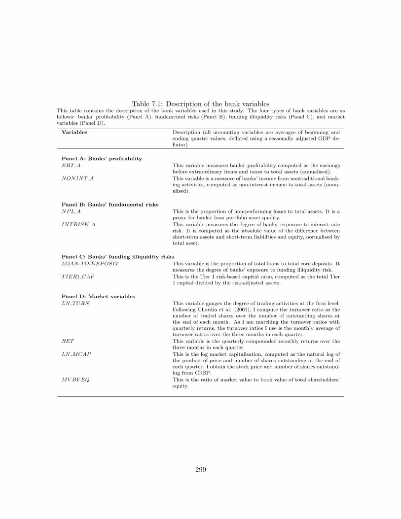
Table 7.1: Description of the bank variablesThis table contains the description of the bank variables used in this study. The four types of bank variables are asfollows: banks’ profitability (Panel A), fundamental risks (Panel B), funding illiquidity risks (Panel C), and marketvariables (Panel D).
Variables Description (all accounting variables are averages of beginning andending quarter values, deflated using a seasonally adjusted GDP de-flator)
Panel A: Banks’ profitability
EBT A This variable measures banks’ profitability computed as the earningsbefore extraordinary items and taxes to total assets (annualised).
NONINT A This variable is a measure of banks’ income from nontraditional bank-ing activities, computed as non-interest income to total assets (annu-alised).
Panel B: Banks’ fundamental risks
NPL A This is the proportion of non-performing loans to total assets. It is aproxy for banks’ loan portfolio asset quality.
INTRISK A This variable measures the degree of banks’ exposure to interest raterisk. It is computed as the absolute value of the difference betweenshort-term assets and short-term liabilities and equity, normalised bytotal asset.
Panel C: Banks’ funding illiquidity risks
LOAN -TO-DEPOSIT This variable is the proportion of total loans to total core deposits. Itmeasures the degree of banks’ exposure to funding illiquidity risk.
TIER1 CAP This is the Tier 1 risk-based capital ratio, computed as the total Tier1 capital divided by the risk-adjusted assets.
Panel D: Market variables
LN TURN This variable gauges the degree of trading activities at the firm level.Following Chordia et al. (2001), I compute the turnover ratio as thenumber of traded shares over the number of outstanding shares atthe end of each month. As I am matching the turnover ratios withquarterly returns, the turnover ratios I use is the monthly average ofturnover ratios over the three months in each quarter.
RET This variable is the quarterly compounded monthly returns over thethree months in each quarter.
LN MCAP This is the log market capitalisation, computed as the natural log ofthe product of price and number of shares outstanding at the end ofeach quarter. I obtain the stock price and number of shares outstand-ing from CRSP.
MVBV EQ This is the ratio of market value to book value of total shareholders’equity.
299
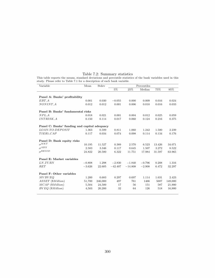
Table 7.2: Summary statisticsThis table reports the means, standard deviations and percentile statistics of the bank variables used in thisstudy. Please refer to Table 7.1 for a description of each bank variable.
Variable Mean Stdev Percentiles
5% 25% Median 75% 95%
Panel A: Banks’ profitability
EBT A 0.001 0.030 −0.055 0.000 0.009 0.016 0.024
NONINT A 0.012 0.012 0.001 0.006 0.010 0.016 0.033
Panel B: Banks’ fundamental risks
NPL A 0.018 0.021 0.001 0.004 0.012 0.025 0.059
INTRISK A 0.150 0.114 0.017 0.060 0.124 0.216 0.375
Panel C: Banks’ funding and capital adequacy
LOAN -TO-DEPOSIT 1.363 0.599 0.811 1.060 1.242 1.500 2.239
TIER1 CAP 0.117 0.034 0.074 0.098 0.114 0.134 0.176
Panel D: Bank equity risks
σMKT 10.195 11.527 0.389 2.570 6.523 13.426 34.071
σABX 2.583 3.346 0.117 0.645 1.507 3.272 8.522
σRESID 24.822 20.580 6.322 11.751 17.984 31.597 63.965
Panel E: Market variables
LN TURN −0.808 1.298 −2.830 −1.840 −0.796 0.208 1.316
RET −3.626 22.605 −42.407 −14.808 −2.908 6.472 32.297
Panel F: Other variables
MVBV EQ 1.200 0.683 0.297 0.697 1.114 1.631 2.423
ASSET ($Million) 51,700 246,000 497 761 1466 5687 149,000
MCAP ($Million) 5,504 24,500 17 56 151 587 21,900
BV EQ ($Million) 4,503 20,200 32 64 126 518 16,900
300
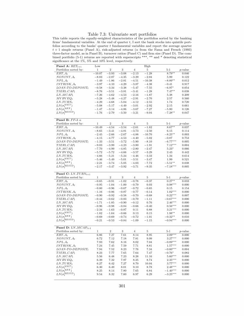
Table 7.3: Univariate sort portfoliosThis table reports the equally-weighted characteristics of the portfolios sorted by the bankingfirms’ fundamental variables. At the end of quarter t, I sort the bank stocks into quintile port-folios according to the banks’ quarter t fundamental variables and report the average quartert + 1 simple returns (Panel A), risk-adjusted returns (α from the Fama and French (1993)three-factor model, as in Panel B), turnover ratios (Panel C) and firm size (Panel D). The com-bined portfolio (5-1) returns are reported with superscripts ***, ** and * denoting statisticalsignificance at the 1%, 5% and 10% level, respectively.
Panel A: RETt+1 Low HighPortfolios sorted by: 1 2 3 4 5 5-1 p-value
EBT At −10.07 −3.93 −3.08 −2.13 −1.28 8.79∗∗ 0.046NONINT At −8.03 −2.87 −4.35 −3.29 −2.04 5.99 0.122NPL At −1.49 −1.86 −2.81 −4.51 −10.38 −8.89∗∗ 0.012INTRISK At −3.97 −4.10 −4.29 −3.87 −4.38 −0.41 0.917LOAN -TO-DEPOSITt −0.58 −3.34 −3.38 −5.47 −7.55 −6.97∗ 0.054TIER1 CAPt −8.76 −3.51 −3.81 −3.41 −1.28 7.47∗∗ 0.038LN MCAPt −7.26 −4.62 −4.53 −2.16 −1.87 5.38 0.209MVBV EQt −5.28 −5.48 −4.27 −2.91 −2.70 2.57 0.560LN TURNt −4.29 −4.68 −5.04 −4.12 −2.55 1.74 0.720LN(σMKT
t ) −5.08 −5.17 −4.49 −3.01 −2.92 2.15 0.661LN(σABX
t ) −1.47 −3.14 −4.86 −3.67 −7.27 −5.80 0.126LN(σRESID
t ) −1.76 −2.79 −3.50 −3.21 −9.04 −7.28∗∗ 0.047
Panel B: FF -3 αPortfolios sorted by: 1 2 3 4 5 5-1 p-value
EBT At −10.49 −4.54 −3.54 −2.61 −1.82 8.67∗∗ 0.037NONINT At −8.65 −3.41 −4.81 −3.73 −2.50 6.15 0.114NPL At −2.45 −2.66 −2.67 −4.88 −10.70 −8.25∗∗ 0.003INTRISK At −4.15 −4.77 −4.53 −4.40 −5.02 −0.87 0.753LOAN -TO-DEPOSITt −1.33 −3.51 −3.72 −5.90 −8.10 −6.77∗∗∗ 0.005TIER1 CAPt −9.03 −3.99 −4.23 −3.80 −1.91 7.12∗∗∗ 0.004LN MCAPt −7.70 −4.99 −4.85 −2.80 −2.47 5.23∗ 0.066MVBV EQt −5.72 −5.72 −4.66 −3.57 −3.29 2.43 0.442LN TURNt −4.66 −5.21 −5.24 −4.46 −3.33 1.34 0.614LN(σMKT
t ) −5.46 −5.49 −5.01 −3.51 −3.47 1.99 0.521LN(σABX
t ) −2.21 −3.74 −5.05 −4.03 −7.72 −5.51∗∗ 0.038LN(σRESID
t ) −2.17 −3.47 −3.92 −3.71 −9.35 −7.18∗∗∗ 0.005
Panel C: LN TURNt+1
Portfolios sorted by: 1 2 3 4 5 5-1 p-value
EBT At −0.65 −0.91 −1.02 −0.78 −0.37 0.27∗∗ 0.033NONINT At −0.95 −1.04 −1.00 −0.79 0.03 0.98∗∗∗ 0.000NPL At −0.80 −0.96 −0.67 −0.72 −0.65 0.15 0.154INTRISK At −1.16 −0.86 −0.87 −0.77 −0.14 1.02∗∗∗ 0.000LOAN -TO-DEPOSITt −0.90 −0.92 −0.58 −0.70 −0.68 0.22∗∗∗ 0.007TIER1 CAPt −0.44 −0.62 −0.83 −0.79 −1.11 −0.67∗∗∗ 0.000LN MCAPt −1.71 −1.85 −0.90 −0.12 0.76 2.46∗∗∗ 0.000MVBV EQt −0.96 −0.98 −0.84 −0.66 −0.40 0.56∗∗∗ 0.000LN TURNt −2.34 −1.63 −0.87 0.11 0.88 3.21∗∗∗ 0.000LN(σMKT
t ) −1.82 −1.64 −0.66 0.13 0.15 1.98∗∗ 0.000LN(σABX
t ) −0.69 −0.69 −0.74 −0.72 −1.01 −0.32∗∗ 0.010LN(σRESID
t ) −0.21 −0.53 −0.84 −1.09 −1.15 −0.94∗∗∗ 0.000
Panel D: LN MCAPt+1
Portfolios sorted by: 1 2 3 4 5 5-1 p-value
EBT At 6.86 7.27 7.61 8.14 8.95 2.09∗∗∗ 0.000NONINT At 6.72 7.12 7.18 7.81 9.99 3.27∗∗∗ 0.000NPL At 7.93 7.62 8.16 8.02 7.04 −0.89∗∗∗ 0.000INTRISK At 7.24 7.45 7.59 7.71 8.81 1.57∗∗∗ 0.000LOAN -TO-DEPOSITt 7.94 7.52 8.23 7.76 7.34 −0.60∗∗∗ 0.004TIER1 CAPt 8.23 7.77 7.65 7.64 7.47 −0.76∗ 0.082LN MCAPt 5.56 6.48 7.23 8.28 11.16 5.60∗∗∗ 0.000MVBV EQt 6.39 7.32 7.97 8.25 8.74 2.35∗∗∗ 0.000LN TURNt 6.27 6.42 7.27 8.70 10.04 3.77∗∗∗ 0.000LN(σMKT
t ) 6.30 6.49 8.01 9.10 8.78 2.48∗∗∗ 0.000LN(σABX
t ) 8.25 8.14 7.80 7.65 6.84 −1.40∗∗∗ 0.000LN(σRESID
t ) 9.54 8.32 7.60 6.97 6.29 −3.25∗∗∗ 0.000
301
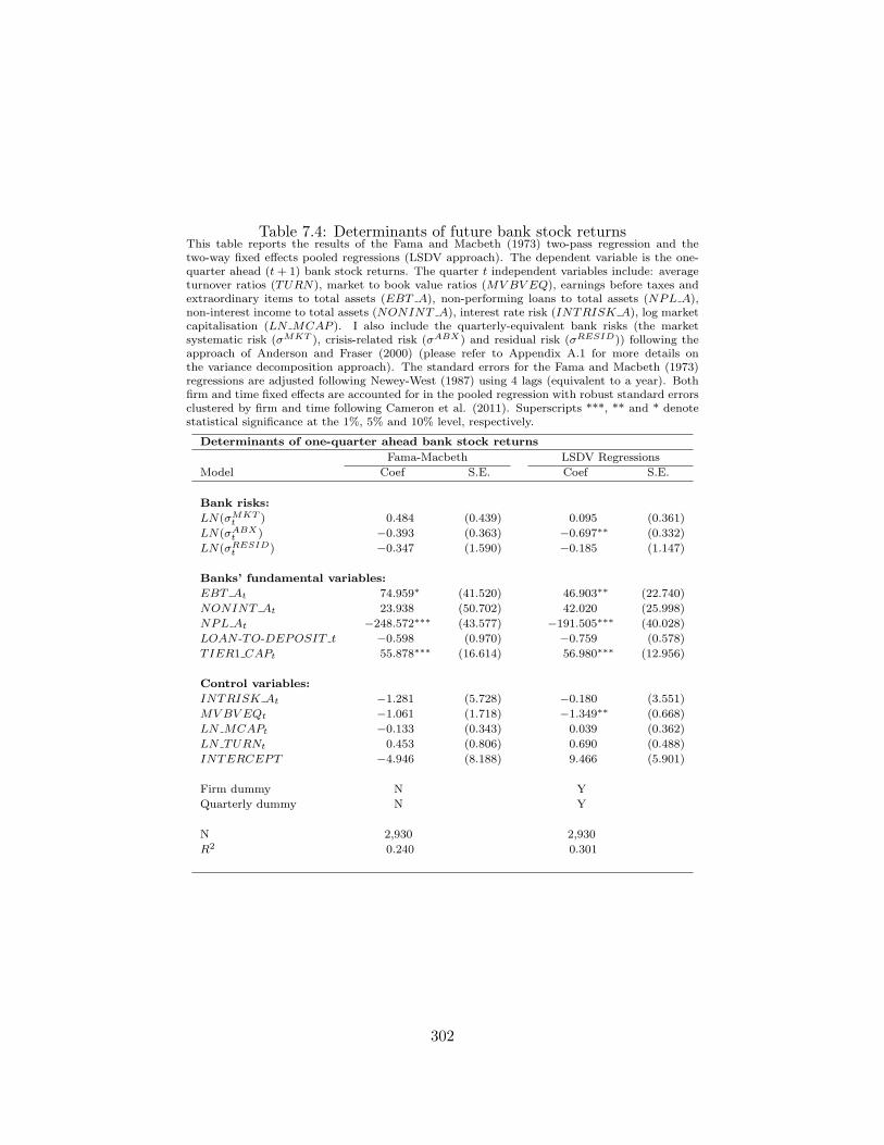
Table 7.4: Determinants of future bank stock returnsThis table reports the results of the Fama and Macbeth (1973) two-pass regression and thetwo-way fixed effects pooled regressions (LSDV approach). The dependent variable is the one-quarter ahead (t+ 1) bank stock returns. The quarter t independent variables include: averageturnover ratios (TURN), market to book value ratios (MVBV EQ), earnings before taxes andextraordinary items to total assets (EBT A), non-performing loans to total assets (NPL A),non-interest income to total assets (NONINT A), interest rate risk (INTRISK A), log marketcapitalisation (LN MCAP ). I also include the quarterly-equivalent bank risks (the marketsystematic risk (σMKT ), crisis-related risk (σABX) and residual risk (σRESID)) following theapproach of Anderson and Fraser (2000) (please refer to Appendix A.1 for more details onthe variance decomposition approach). The standard errors for the Fama and Macbeth (1973)regressions are adjusted following Newey-West (1987) using 4 lags (equivalent to a year). Bothfirm and time fixed effects are accounted for in the pooled regression with robust standard errorsclustered by firm and time following Cameron et al. (2011). Superscripts ***, ** and * denotestatistical significance at the 1%, 5% and 10% level, respectively.
Determinants of one-quarter ahead bank stock returns
Fama-Macbeth LSDV Regressions
Model Coef S.E. Coef S.E.
Bank risks:
LN(σMKTt ) 0.484 (0.439) 0.095 (0.361)
LN(σABXt ) −0.393 (0.363) −0.697∗∗ (0.332)
LN(σRESIDt ) −0.347 (1.590) −0.185 (1.147)
Banks’ fundamental variables:
EBT At 74.959∗ (41.520) 46.903∗∗ (22.740)
NONINT At 23.938 (50.702) 42.020 (25.998)
NPL At −248.572∗∗∗ (43.577) −191.505∗∗∗ (40.028)
LOAN -TO-DEPOSIT t −0.598 (0.970) −0.759 (0.578)
TIER1 CAPt 55.878∗∗∗ (16.614) 56.980∗∗∗ (12.956)
Control variables:
INTRISK At −1.281 (5.728) −0.180 (3.551)
MVBV EQt −1.061 (1.718) −1.349∗∗ (0.668)
LN MCAPt −0.133 (0.343) 0.039 (0.362)
LN TURNt 0.453 (0.806) 0.690 (0.488)
INTERCEPT −4.946 (8.188) 9.466 (5.901)
Firm dummy N Y
Quarterly dummy N Y
N 2,930 2,930
R2 0.240 0.301
302
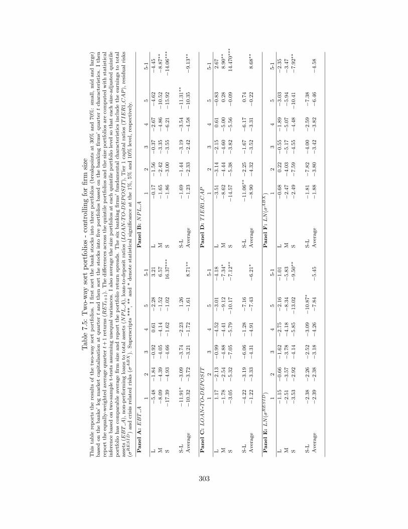
Tab
le7.5:Two-w
aysort
portfolios-controllingforfirm
size
This
table
reportsth
eresu
ltsofth
etw
o-w
aysort
portfolios.
Ifirstsort
thebankstock
sinto
threeportfolios(b
reakpoints
at30%
and70%:sm
all,mid
andlarge)
basedonth
ebanks’
logmarket
capitalisationatquarter
tandth
ensort
thestock
sinto
fiveportfoliosbasedonth
ebankingfirm
s’quarter
tch
aracteristics.Ith
enreport
theeq
ually-w
eightedaveragequarter
t+1retu
rns(R
ETt+
1).
Thedifferen
cesacross
thequintile
portfoliosandth
esize
portfoliosare
computedwithstatistical
inference
basedontw
o-sample
t-testsassuminguneq
ualvariances.
Ialsoaverageth
esize
portfoliosatea
chquintile
portfoliolevel
soth
atea
chsize-adjusted
quintile
portfoliohasco
mparable
averagefirm
size
andreport
theportfolioretu
rnsp
reads.
Thesixbankingfirm
s’fundamen
talch
aracteristics
includeth
eea
rningsto
total
assets(E
BT
A),
non-perform
ingloansto
totalassets(N
PL
A),
loan-to-dep
ositratios(L
OAN-T
O-D
EPOSIT),
Tier1ca
pitalratios(T
IER1CAP),
residualrisks
(σRESID)andcrisis
relatedrisks(σ
ABX).
Superscripts
***,**and*den
ote
statisticalsignifica
nce
atth
e1%,5%
and10%
level,resp
ectively.
PanelA:EBT
APanelB:NPL
A
12
34
55-1
12
34
55-1
L−5.48
−1.84
−0.92
0.61
−2.28
3.21
L−0.17
−1.56
−0.37
−2.67
−4.62
−4.45
M−8.09
−4.39
−4.05
−4.14
−1.52
6.57
M−1.65
−2.42
−3.35
−4.86
−10.52
−8.87∗∗
S−17.39
−4.93
−4.66
−1.62
−1.02
16.37∗∗
∗S
−1.86
−3.00
−3.55
−6.21
−15.92
−14.06∗∗
∗
S-L
−11.91∗
−3.09
−3.74
−2.23
1.26
S-L
−1.69
−1.44
−3.19
−3.54
−11.31∗∗
Average
−10.32
−3.72
−3.21
−1.72
−1.61
8.71∗∗
Average
−1.23
−2.33
−2.42
−4.58
−10.35
−9.13∗∗
PanelC:LOAN-T
O-D
EPOSIT
PanelD:TIER1CAP
12
34
55-1
12
34
55-1
L1.17
−2.13
−0.99
−4.52
−3.01
−4.18
L−3.51
−3.14
−2.15
0.61
−0.83
2.67
M−1.78
−2.54
−4.88
−4.41
−9.12
−7.34∗
M−8.62
−4.44
−4.60
−5.00
0.28
8.90∗∗
S−3.05
−5.32
−7.05
−5.79
−10.17
−7.12∗∗
S−14.57
−5.38
−3.82
−5.56
−0.09
14.470∗∗
∗
S-L
−4.22
−3.19
−6.06
−1.28
−7.16
S-L
−11.06∗∗
−2.25
−1.67
−6.17
0.74
Average
−1.22
−3.33
−4.31
−4.91
−7.43
−6.21∗
Average
−8.90
−4.32
−3.52
−3.31
−0.22
8.68∗∗
PanelE:LN(σ
RESID)
PanelF:LN(σ
ABX)
12
34
55-1
12
34
55-1
L−1.15
−0.66
−1.62
−2.75
−2.16
−1.01
L−0.68
0.22
−0.55
−1.89
−3.03
−2.35
M−2.51
−3.57
−3.78
−4.18
−8.34
−5.83
M−2.47
−4.03
−5.17
−5.07
−5.94
−3.47
S−3.53
−2.92
−4.14
−5.85
−13.02
−9.50∗∗
S−2.49
−7.59
−4.55
−4.48
−10.41
−7.92∗∗
S-L
−2.38
−2.26
−2.52
−3.09
−10.87∗
S-L
−1.81
−7.82
−4.00
−2.59
−7.38
Average
−2.39
−2.38
−3.18
−4.26
−7.84
−5.45
Average
−1.88
−3.80
−3.42
−3.82
−6.46
−4.58
303
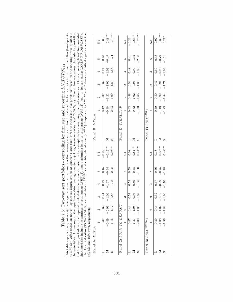
Tab
le7.6:
Two-way
sort
portfolios-controllingforfirm
size
andreportingLNTURN
t+1
This
table
reportsth
equarter
t+
1averagetu
rnover
ratiosbasedonth
etw
o-w
aysort
portfolios.
Ifirstsort
thebankstock
sinto
threeportfolios(b
reakpoints
at30%
and
70%)based
on
banks’
logmarket
capitalisation
atquarter
tand
then
sort
thestock
sinto
fiveportfoliosbased
on
thebankingfirm
s’quarter
tch
aracteristics.
Ith
enreport
theeq
ually-w
eighted
averagequarter
t+
1logtu
rnover
ratios(L
NTURN
t+1).
Thedifferen
cesacross
thequintile
portfolios
andth
esize
portfoliosare
computedwithstatisticalinference
basedontw
o-sample
t-testsassuminguneq
ualvariances.
Thesixbankingfirm
s’fundamen
tal
characteristics
includeth
eea
rningsto
totalassets(E
BT
A),
non-perform
ingloansto
totalassets(N
PL
A),
loan-to-dep
ositratios(L
OAN-T
O-D
EPOSIT),
Tier1ca
pitalratios(T
IER1CAP),
residualrisks(σ
RESID)andcrisis
relatedrisks(σ
ABX).
Superscripts
***,**and*den
ote
statisticalsignifica
nce
atth
e1%,5%
and10%
level,resp
ectively.
PanelA:EBT
APanelB:NPL
A
12
34
55-1
12
34
55-1
L0.67
0.62
0.44
0.49
0.45
−0.22
L0.42
0.37
0.62
0.71
0.46
0.03
M−0.49
−0.99
−1.06
−1.27
−0.94
−0.45∗∗
∗M
−0.98
−1.22
−1.06
−1.03
−0.49
0.48∗∗
∗
S−1.16
−1.72
−1.86
−1.98
−2.08
−0.93∗∗
∗S
−2.03
−1.99
−1.89
−1.63
−1.24
0.79∗∗
∗
PanelC:LOAN-T
O-D
EPOSIT
PanelD:TIER1CAP
12
34
55-1
12
34
55-1
L0.47
0.44
0.54
0.59
0.55
0.08
L0.63
0.58
0.54
0.48
0.41
−0.22
M−1.37
−1.08
−0.96
−0.89
−0.55
0.81∗∗
∗M
−0.72
−1.02
−0.94
−0.90
−1.35
−0.63∗∗
∗
S−2.00
−1.86
−1.67
−1.66
−1.60
0.41∗∗
∗S
−1.30
−1.65
−1.88
−1.89
−2.06
−0.75∗∗
∗
PanelE:LN(σ
RESID)
PanelF:LN(σ
ABX)
12
34
55-1
12
34
55-1
L0.39
0.44
0.52
0.57
0.56
0.18
L0.50
0.50
0.47
0.50
0.48
−0.02
M−1.08
−1.02
−1.12
−0.99
−0.75
0.33∗∗
∗M
−1.18
−0.99
−0.94
−0.95
−0.79
0.39∗∗
∗
S−1.96
−1.89
−1.90
−1.70
−1.48
0.48∗∗
∗S
−1.83
−1.84
−1.71
−1.99
−1.61
0.21∗
304
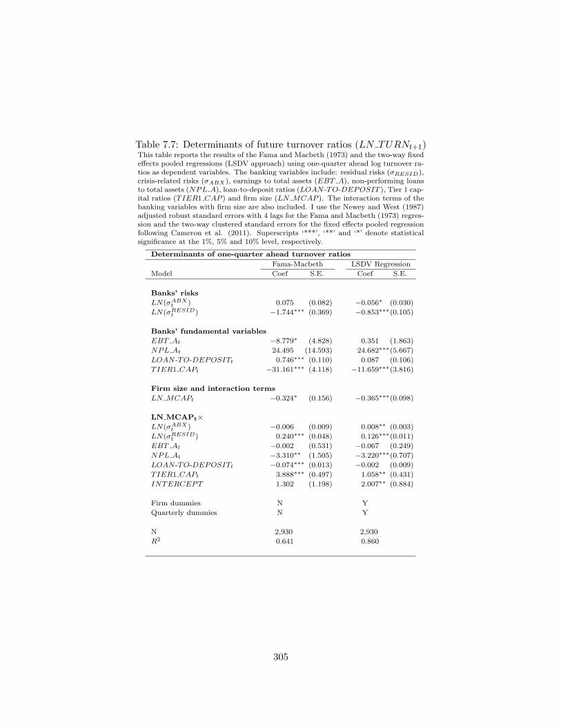
Table 7.7: Determinants of future turnover ratios (LN TURNt+1)This table reports the results of the Fama and Macbeth (1973) and the two-way fixedeffects pooled regressions (LSDV approach) using one-quarter ahead log turnover ra-tios as dependent variables. The banking variables include: residual risks (σRESID),crisis-related risks (σABX), earnings to total assets (EBT A), non-performing loansto total assets (NPL A), loan-to-deposit ratios (LOAN -TO-DEPOSIT ), Tier 1 cap-ital ratios (TIER1 CAP ) and firm size (LN MCAP ). The interaction terms of thebanking variables with firm size are also included. I use the Newey and West (1987)adjusted robust standard errors with 4 lags for the Fama and Macbeth (1973) regres-sion and the two-way clustered standard errors for the fixed effects pooled regressionfollowing Cameron et al. (2011). Superscripts ‘***’, ‘**’ and ‘*’ denote statisticalsignificance at the 1%, 5% and 10% level, respectively.
Determinants of one-quarter ahead turnover ratios
Fama-Macbeth LSDV Regression
Model Coef S.E. Coef S.E.
Banks’ risks
LN(σABXt ) 0.075 (0.082) −0.056∗ (0.030)
LN(σRESIDt ) −1.744∗∗∗ (0.369) −0.853∗∗∗(0.105)
Banks’ fundamental variables
EBT At −8.779∗ (4.828) 0.351 (1.863)
NPL At 24.495 (14.593) 24.682∗∗∗(5.667)
LOAN -TO-DEPOSITt 0.746∗∗∗ (0.110) 0.087 (0.106)
TIER1 CAPt −31.161∗∗∗ (4.118) −11.659∗∗∗(3.816)
Firm size and interaction terms
LN MCAPt −0.324∗ (0.156) −0.365∗∗∗(0.098)
LN MCAPt×LN(σABX
t ) −0.006 (0.009) 0.008∗∗ (0.003)
LN(σRESIDt ) 0.240∗∗∗ (0.048) 0.126∗∗∗(0.011)
EBT At −0.002 (0.531) −0.067 (0.249)
NPL At −3.310∗∗ (1.505) −3.220∗∗∗(0.707)
LOAN -TO-DEPOSITt −0.074∗∗∗ (0.013) −0.002 (0.009)
TIER1 CAPt 3.888∗∗∗ (0.497) 1.058∗∗ (0.431)
INTERCEPT 1.302 (1.198) 2.007∗∗ (0.884)
Firm dummies N Y
Quarterly dummies N Y
N 2,930 2,930
R2 0.641 0.860
305
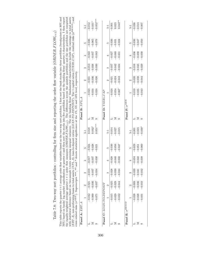
Tab
le7.8:
Two-way
sort
portfolios-controllingforfirm
size
andreportingtheorder
flow
variable
(ORDERFLOW
t+1)
This
table
reportsth
equarter
t+1averageord
erflow
variablesbasedonth
etw
o-w
aysort
portfolios.
Ifirstsort
thebankstock
sinto
threeportfolios(b
reakpoints
at30%
and
70%)basedonbanks’
logmarket
capitalisationatquarter
tandth
ensort
thestock
sinto
fiveportfoliosbasedonth
ebankingfirm
s’quarter
tch
aracteristics.Ith
enreport
theeq
ually-w
eighted
averagequarter
t+
1ord
erflow
mea
sures(O
RDER
FLOW
t+1).
Thedifferen
cesacross
thequintile
portfoliosand
thesize
portfoliosare
computed
with
statisticalinference
based
on
two-sample
t-testsassuminguneq
ualvariances.
Thesixbankingfirm
s’fundamen
talch
aracteristics
includeth
eea
rningsto
totalassets
(EBT
A),
non-perform
ingloansto
totalassets(N
PL
A),
loan-to-dep
ositratios(L
OAN-T
O-D
EPOSIT),
Tier1ca
pitalratios(T
IER1CAP),
residualrisks(σ
RESID)and
crisis
relatedrisks(σ
ABX).
Superscripts
***,**and*den
ote
statisticalsignifica
nce
atth
e1%,5%
and10%
level,resp
ectively.
PanelA:EBT
APanelB:NPL
A
12
34
55-1
12
34
55-1
L−0.042
−0.021
−0.019
−0.017
−0.024
0.018
L−0.023
−0.031
−0.013
−0.022
−0.036
−0.012
M−0.060
−0.030
−0.037
−0.037
−0.028
0.032∗
M−0.034
−0.036
−0.026
−0.037
−0.065
−0.031∗
S−0.071
−0.037
−0.034
−0.030
−0.021
0.051∗∗
∗S
−0.024
−0.026
−0.030
−0.043
−0.076
−0.052∗∗
∗
PanelC:LOAN-T
O-D
EPOSIT
PanelD:TIER1CAP
12
34
55-1
12
34
55-1
L−0.015
−0.025
−0.028
−0.028
−0.030
−0.014
L−0.024
−0.021
−0.037
−0.027
−0.026
−0.001
M−0.029
−0.029
−0.039
−0.040
−0.056
−0.027
M−0.054
−0.024
−0.042
−0.040
−0.031
0.023
S−0.032
−0.044
−0.044
−0.040
−0.047
−0.015
S−0.067
−0.043
−0.034
−0.031
−0.024
0.043∗∗
PanelE:σRESID
PanelF:σABX
12
34
55-1
12
34
55-1
L−0.028
−0.009
−0.020
−0.034
−0.029
−0.001
L−0.010
−0.020
−0.016
−0.036
−0.036
−0.026
M−0.028
−0.036
−0.041
−0.040
−0.051
−0.023
M−0.035
−0.038
−0.045
−0.030
−0.047
−0.013
S−0.031
−0.033
−0.032
−0.039
−0.060
−0.030∗
S−0.043
−0.044
−0.029
−0.030
−0.050
−0.007
306
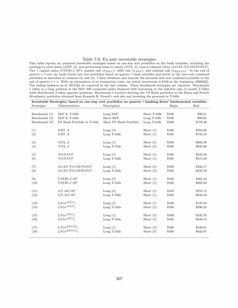
Table 7.9: Ex ante investable strategiesThis table reports my proposed investable strategies based on one-way sort portfolios on the bank variables, including theearnings to total assets (EBT A), non-performing loans to assets (NPL A), loan-to-deposit ratios (LOAN -TO-DEPOSIT ),Tier 1 capital ratios (TIER1 CAP ), market risk (σMKT ), ABX risk (σABX), and residual risk (σRESID). At the end ofquarter t, I sort my bank stocks into five portfolios based on quarter t bank variables and invest in the zero-cost combinedportfolios as described in columns (3) and (4). I then rebalance and reinvest the proceeds into new combined portfolio at theend of quarter t + 1. With an assumption of no transaction costs, my initial investment is $100 at the beginning (2006Q2).The ending balances as at 2011Q4 are reported in the last column. Three benchmark strategies are reported. Benchmark1 refers to a long position in the S&P 500 composite index financed with borrowing at the risk-free rate (3 month T-bills)while Benchmark 2 takes opposite positions. Benchmark 3 involves shorting the US Bank portfolios in the Fama and French49-industry portfolios obtained from Kenneth R. French’s web site and investing the proceeds in T-bills.
Investable Strategies, based on one-way sort portfolios on quarter t banking firms’ fundamental variables
Strategies Characteristics Description Begin End
Benchmark (1) S&P & T-bills Long S&P Short T-bills $100 $90.51
Benchmark (2) S&P & T-bills Short S&P Long T-bills $100 $88.65
Benchmark (3) FF Bank Portfolio & T-bills Short FF Bank Portfolio Long T-bills $100 $179.46
(1) EBT A Long (5) Short (1) $100 $582.80
(2) EBT A Long T-bills Short (1) $100 $743.19
(3) NPL A Long (1) Short (5) $100 $602.38
(4) NPL A Long T-bills Short (5) $100 $832.06
(5) NONINT Long (5) Short (1) $100 $333.58
(6) NONINT Long T-bills Short (1) $100 $515.82
(7) LOAN -TO-DEPOSIT Long (1) Short (5) $100 $422.17
(8) LOAN -TO-DEPOSIT Long T-bills Short (5) $100 $456.78
(9) TIER1 CAP Long (5) Short (1) $100 $465.42
(10) TIER1 CAP Long T-bills Short (1) $100 $605.63
(11) LN MCAP Long (5) Short (1) $100 $255.72
(12) LN MCAP Long T-bills Short (1) $100 $450.42
(13) LN(σMKT ) Long (5) Short (1) $100 $137.04
(14) LN(σMKT ) Long T-bills Short (1) $100 $290.33
(15) LN(σABX) Long (1) Short (5) $100 $332.76
(16) LN(σABX) Long T-bills Short (5) $100 $438.54
(17) LN(σRESID) Long (1) Short (5) $100 $440.61
(18) LN(σRESID) Long T-bills Short (5) $100 $643.97
307
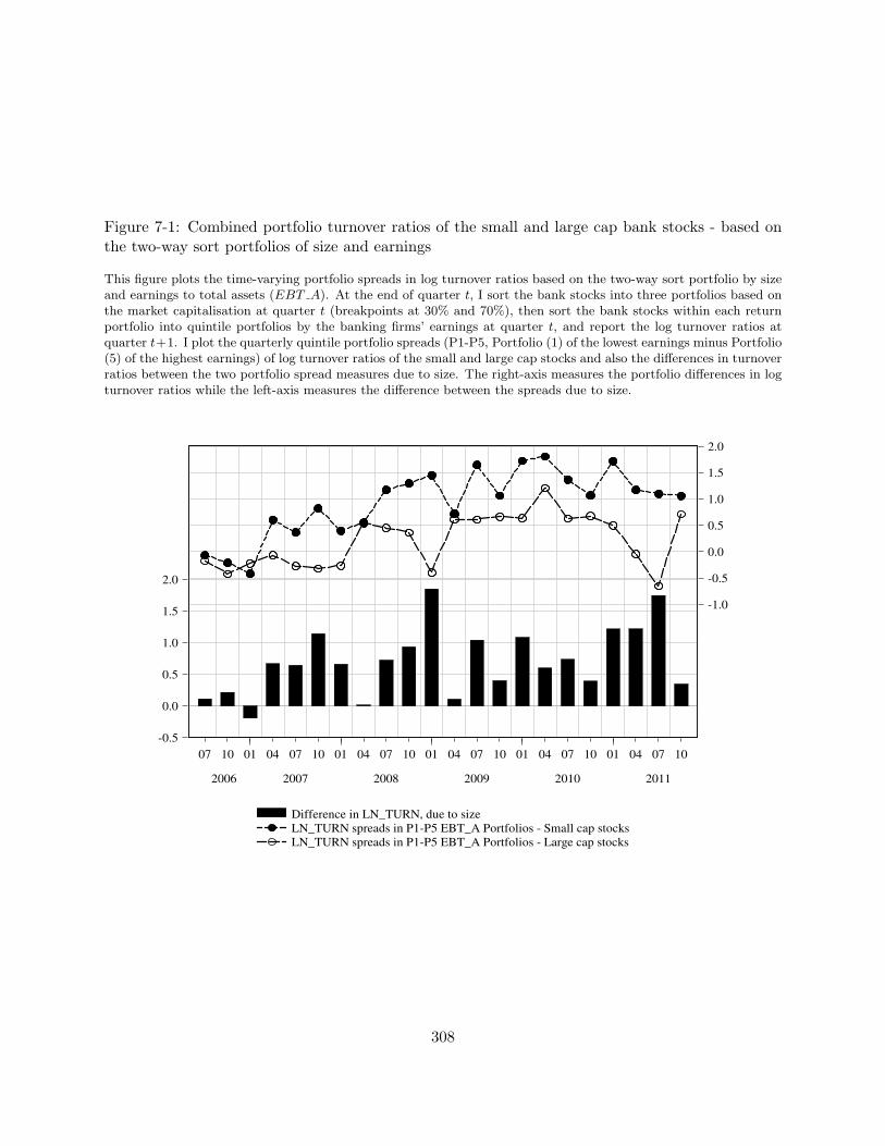
Figure 7-1: Combined portfolio turnover ratios of the small and large cap bank stocks - based onthe two-way sort portfolios of size and earnings
This figure plots the time-varying portfolio spreads in log turnover ratios based on the two-way sort portfolio by sizeand earnings to total assets (EBT A). At the end of quarter t, I sort the bank stocks into three portfolios based onthe market capitalisation at quarter t (breakpoints at 30% and 70%), then sort the bank stocks within each returnportfolio into quintile portfolios by the banking firms’ earnings at quarter t, and report the log turnover ratios atquarter t+1. I plot the quarterly quintile portfolio spreads (P1-P5, Portfolio (1) of the lowest earnings minus Portfolio(5) of the highest earnings) of log turnover ratios of the small and large cap stocks and also the differences in turnoverratios between the two portfolio spread measures due to size. The right-axis measures the portfolio differences in logturnover ratios while the left-axis measures the difference between the spreads due to size.
-0.5
0.0
0.5
1.0
1.5
2.0
-1.0
-0.5
0.0
0.5
1.0
1.5
2.0
07 10 01 04 07 10 01 04 07 10 01 04 07 10 01 04 07 10 01 04 07 10
2006 2007 2008 2009 2010 2011
Difference in LN_TURN, due to size
LN_TURN spreads in P1-P5 EBT_A Portfolios - Small cap stocks
LN_TURN spreads in P1-P5 EBT_A Portfolios - Large cap stocks
308
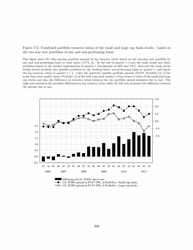
Figure 7-2: Combined portfolio turnover ratios of the small and large cap bank stocks - based onthe two-way sort portfolios of size and non-performing loans
This figure plots the time-varying portfolio spreads in log turnover ratios based on the two-way sort portfolio bysize and non-performing loans to total assets (NPL A). At the end of quarter t, I sort the bank stocks into threeportfolios based on the market capitalisation at quarter t (breakpoints at 30% and 70%), then sort the bank stockswithin return portfolio into quintile portfolios by the banking firms’ non-performing loans at quarter t, and reportthe log turnover ratios at quarter t + 1. I plot the quarterly quintile portfolio spreads (P5-P1, Portfolio (5) of theworst loan asset quality minus Portfolio (1) of the best loan asset quality) of log turnover ratios of the small and largecap stocks and also the differences in turnover ratios between the two portfolio spread measures due to size. Theright-axis measures the portfolio differences in log turnover ratios while the left-axis measures the difference betweenthe spreads due to size.
-0.5
0.0
0.5
1.0
1.5
2.0
2.5
-2.0
-1.0
0.0
1.0
2.0
3.0
07 10 01 04 07 10 01 04 07 10 01 04 07 10 01 04 07 10 01 04 07 10
2006 2007 2008 2009 2010 2011
Difference in LN_TURN, due to size
LN_TURN spreads in P5-P1 NPL_A Portfolios - Small cap stocks
LN_TURN spreads in P5-P1 NPL_A Portfolios - Large cap stocks
309
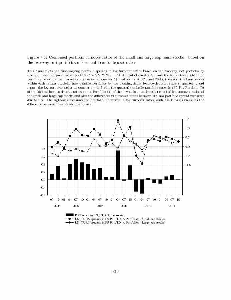
Figure 7-3: Combined portfolio turnover ratios of the small and large cap bank stocks - based onthe two-way sort portfolios of size and loan-to-deposit ratios
This figure plots the time-varying portfolio spreads in log turnover ratios based on the two-way sort portfolio bysize and loan-to-deposit ratios (LOAN -TO-DEPOSIT ). At the end of quarter t, I sort the bank stocks into threeportfolios based on the market capitalisation at quarter t (breakpoints at 30% and 70%), then sort the bank stockswithin each return portfolio into quintile portfolios by the banking firms’ loan-to-deposit ratios at quarter t, andreport the log turnover ratios at quarter t + 1. I plot the quarterly quintile portfolio spreads (P5-P1, Portfolio (5)of the highest loan-to-deposit ratios minus Portfolio (1) of the lowest loan-to-deposit ratios) of log turnover ratios ofthe small and large cap stocks and also the differences in turnover ratios between the two portfolio spread measuresdue to size. The right-axis measures the portfolio differences in log turnover ratios while the left-axis measures thedifference between the spreads due to size.
-0.8
-0.4
0.0
0.4
0.8
1.2
1.6
-1.0
-0.5
0.0
0.5
1.0
1.5
07 10 01 04 07 10 01 04 07 10 01 04 07 10 01 04 07 10 01 04 07 10
2006 2007 2008 2009 2010 2011
Difference in LN_TURN, due to size
LN_TURN spreads in P5-P1 LTD_A Portfolios - Small cap stocks
LN_TURN spreads in P5-P1 LTD_A Portfolios - Large cap stocks
310
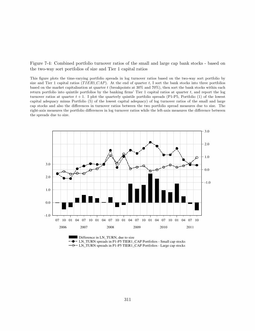
Figure 7-4: Combined portfolio turnover ratios of the small and large cap bank stocks - based onthe two-way sort portfolios of size and Tier 1 capital ratios
This figure plots the time-varying portfolio spreads in log turnover ratios based on the two-way sort portfolio bysize and Tier 1 capital ratios (TIER1 CAP ). At the end of quarter t, I sort the bank stocks into three portfoliosbased on the market capitalisation at quarter t (breakpoints at 30% and 70%), then sort the bank stocks within eachreturn portfolio into quintile portfolios by the banking firms’ Tier 1 capital ratios at quarter t, and report the logturnover ratios at quarter t + 1. I plot the quarterly quintile portfolio spreads (P1-P5, Portfolio (1) of the lowestcapital adequacy minus Portfolio (5) of the lowest capital adequacy) of log turnover ratios of the small and largecap stocks and also the differences in turnover ratios between the two portfolio spread measures due to size. Theright-axis measures the portfolio differences in log turnover ratios while the left-axis measures the difference betweenthe spreads due to size.
-1.0
0.0
1.0
2.0
3.0
-1.0
0.0
1.0
2.0
3.0
07 10 01 04 07 10 01 04 07 10 01 04 07 10 01 04 07 10 01 04 07 10
2006 2007 2008 2009 2010 2011
Difference in LN_TURN, due to size
LN_TURN spreads in P1-P5 TIER1_CAP Portfolios - Small cap stocks
LN_TURN spreads in P1-P5 TIER1_CAP Portfolios - Large cap stocks
311
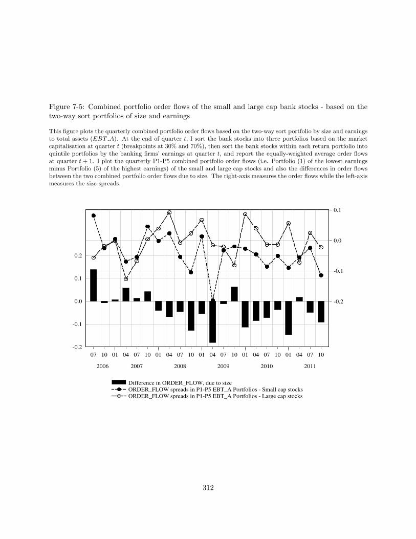
Figure 7-5: Combined portfolio order flows of the small and large cap bank stocks - based on thetwo-way sort portfolios of size and earnings
This figure plots the quarterly combined portfolio order flows based on the two-way sort portfolio by size and earningsto total assets (EBT A). At the end of quarter t, I sort the bank stocks into three portfolios based on the marketcapitalisation at quarter t (breakpoints at 30% and 70%), then sort the bank stocks within each return portfolio intoquintile portfolios by the banking firms’ earnings at quarter t, and report the equally-weighted average order flowsat quarter t + 1. I plot the quarterly P1-P5 combined portfolio order flows (i.e. Portfolio (1) of the lowest earningsminus Portfolio (5) of the highest earnings) of the small and large cap stocks and also the differences in order flowsbetween the two combined portfolio order flows due to size. The right-axis measures the order flows while the left-axismeasures the size spreads.
-0.2
-0.1
0.0
0.1
0.2
-0.2
-0.1
0.0
0.1
07 10 01 04 07 10 01 04 07 10 01 04 07 10 01 04 07 10 01 04 07 10
2006 2007 2008 2009 2010 2011
Difference in ORDER_FLOW, due to size
ORDER_FLOW spreads in P1-P5 EBT_A Portfolios - Small cap stocks
ORDER_FLOW spreads in P1-P5 EBT_A Portfolios - Large cap stocks
312
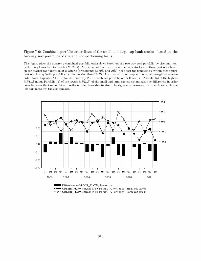
Figure 7-6: Combined portfolio order flows of the small and large cap bank stocks - based on thetwo-way sort portfolios of size and non-performing loans
This figure plots the quarterly combined portfolio order flows based on the two-way sort portfolio by size and non-performing loans to total assets (NPL A). At the end of quarter t, I sort the bank stocks into three portfolios basedon the market capitalisation at quarter t (breakpoints at 30% and 70%), then sort the bank stocks within each returnportfolio into quintile portfolios by the banking firms’ NPL A at quarter t, and report the equally-weighted averageorder flows at quarter t+1. I plot the quarterly P5-P1 combined portfolio order flows (i.e. Portfolio (5) of the highestNPL A minus Portfolio (1) of the lowest NPL A) of the small and large cap stocks and also the differences in orderflows between the two combined portfolio order flows due to size. The right-axis measures the order flows while theleft-axis measures the size spreads.
-0.3
-0.2
-0.1
0.0
0.1
0.2
-0.2
-0.1
0.0
0.1
0.2
07 10 01 04 07 10 01 04 07 10 01 04 07 10 01 04 07 10 01 04 07 10
2006 2007 2008 2009 2010 2011
Difference in ORDER_FLOW, due to size
ORDER_FLOW spreads in P5-P1 NPL_A Portfolios - Small cap stocks
ORDER_FLOW spreads in P5-P1 NPL_A Portfolios - Large cap stocks
313
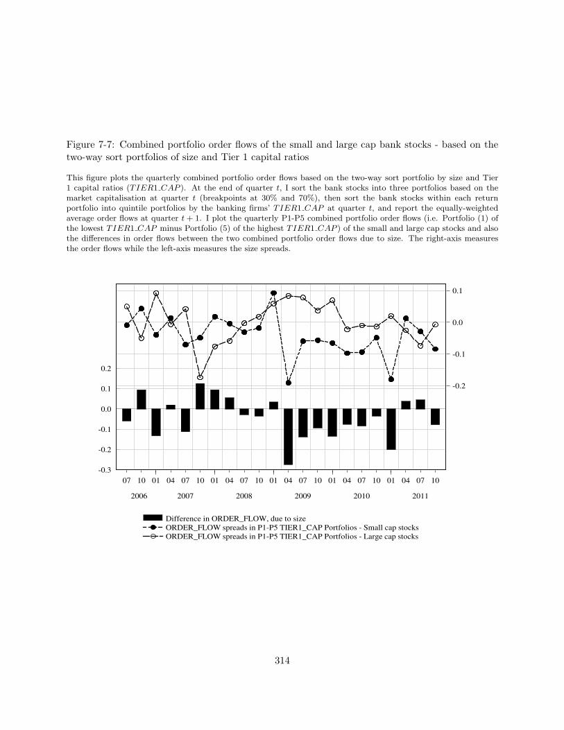
Figure 7-7: Combined portfolio order flows of the small and large cap bank stocks - based on thetwo-way sort portfolios of size and Tier 1 capital ratios
This figure plots the quarterly combined portfolio order flows based on the two-way sort portfolio by size and Tier1 capital ratios (TIER1 CAP ). At the end of quarter t, I sort the bank stocks into three portfolios based on themarket capitalisation at quarter t (breakpoints at 30% and 70%), then sort the bank stocks within each returnportfolio into quintile portfolios by the banking firms’ TIER1 CAP at quarter t, and report the equally-weightedaverage order flows at quarter t + 1. I plot the quarterly P1-P5 combined portfolio order flows (i.e. Portfolio (1) ofthe lowest TIER1 CAP minus Portfolio (5) of the highest TIER1 CAP ) of the small and large cap stocks and alsothe differences in order flows between the two combined portfolio order flows due to size. The right-axis measuresthe order flows while the left-axis measures the size spreads.
-0.3
-0.2
-0.1
0.0
0.1
0.2
-0.2
-0.1
0.0
0.1
07 10 01 04 07 10 01 04 07 10 01 04 07 10 01 04 07 10 01 04 07 10
2006 2007 2008 2009 2010 2011
Difference in ORDER_FLOW, due to size
ORDER_FLOW spreads in P1-P5 TIER1_CAP Portfolios - Small cap stocks
ORDER_FLOW spreads in P1-P5 TIER1_CAP Portfolios - Large cap stocks
314
Chapter 8
Conclusions
8.1 Introduction
The recent 2007 to 2009 financial crisis presents an ideal opportunity to study contagion for a
number of reasons. First, it has clear-cut origins; that is, the subprime mortgage market and the
structured finance market. Second, the recent financial crisis differs from previous crisis events in
that it was characterised by significant financial innovations and by securitisation. An update in
the empirical literature is essential for an understanding of the topical issues in today’s financial
world. Third, it is observed that financial stocks were traded more intensely during the recent
crisis, which is consistent with a possible ‘flight-to-safety’ phenomenon (Longstaff, 2010). The
recent crisis allows us to closely examine the trading patterns and stock performance in relation
to the ‘flight-to-safety’ phenomenon, and reveals how investors made their investment or ‘flight’
decisions during the crisis. Fourth, it is widely-acknowledged that the recent financial crisis was
characterised by severe funding and market illiquidity. This presents ideal conditions for testing the
relation between funding and market illiquidity as proposed in the seminal work by Brunnermeier
and Pedersen (2009). It also presents ideal conditions for studying the role of illiquidity in contagion
transmission.
In this thesis, I have provided a detailed overview of the subprime and the subsequent global
financial crises in relation to the ending of the US housing bubble, the securitisation process, the
reinforcing liquidity spiral between funding and market illiquidity, and the failure of the structured
finance market. I have then reviewed the contagion literature and addressed a few important
issues, including the widespread disagreement of working definitions, the causes of contagion and
315
the empirical methodologies, followed by a summary of the empirical evidence.
Over the past decade, the structured finance market has grown substantially and it has become
one of the largest fixed income markets in the US. Despite its increasing importance to financial
stability, little empirical work has been done to examine the role of the structured finance market
in the context of contagion in the recent financial crisis. I fill this gap by offering a comprehensive
empirical investigation of the spillovers of shocks from the structured finance market indices to a
number of international markets. More importantly, I formulate my contagion tests within an asset
pricing framework and test formally for any significant increase in the linkages between individual
stocks and the ABX innovations during the crisis, thus contributing to both the contagion and
asset pricing literature. I then examine closely the role played by the US BHCs in the recent
crisis and identify the determinants of banks’ equity risks and future stock returns using a set
of bank-specific asset composition and fundamental variables. In addition, I contribute to the
literature by discovering the link between bank stock return predictability and investors’ ‘fire sale’
or ‘flight-to-safety’ phenomena during the recent crisis.
8.2 Synthesis of my empirical findings
First, I extend Longstaff’s (2010) investigation to an international market perspective and test for
contagion from the US structured finance market to the G5 international markets. Using weekly
frequency data, my analysis shows that the shocks from the structured finance market translated
into subsequent declines in the international markets, which is consistent with contagion. I find
strong support for the contagion transmission via the funding liquidity and risk premia channels in
that the negative shocks from the ABX indices led to subsequent higher trading intensity among
financial stocks (in the US, UK, and France) relative to the market, widening of interest rate swap
spreads (in all G5 countries) and heightened comovements between domestic equity and government
bond market index returns (in all G5 countries except Germany). In addition, the evidence suggests
possible ‘flight-to-safety’ from domestic equity to government bond markets, as evinced by the
negative conditional correlations throughout the subprime and global crises. I check the robustness
of my findings by estimating VAR models using daily data and document strong evidence of ‘short-
lived’ contagion (as defined by Kaminsky et al. (2003)) travelling from the ABX indices into the
international markets during both the subprime and global crises. The main implication is that
316
shocks might have been transmitted via the arrival of market news, which is consistent with the
information transmission channel and is in contrast to the conclusion of Longstaff (2010).
To control for the possible simultaneous contagion from the other US markets to the G5 inter-
national markets, I augment the set of exogenous regressors with a number of major US market
variables in addition to the ABX indices and re-estimate the daily VAR models. Qualitatively
similar evidence of contagion from the ABX indices is documented during the subprime crisis while
the lagged US S&P 500 composite index returns and US government bond index returns have been
found to possess significant predictive ability over the international market returns. I also find that
the US lagged ABCP yield spreads, which represented shocks related to funding illiquidity and the
performance of the structured securities market in the US, predicted significantly the international
market returns during the global crisis. The evidence again suggests the importance of funding
illiquidity in shock propagation across the international markets during the recent crisis.
In summary, the evidence presented supports the conventional view that the family of ABX in-
dices was an important class of risk barometer during the recent crisis. The significant predictability
of the ABX indices over the international market returns can alternatively be interpreted as ev-
idence that investors had actively traded on the past performance of the ABX indices while the
price discovery in general takes days rather than weeks. In addition, my results also highlight the
important role of US markets in predicting the international market returns in that traders might
be able to exploit the US market information to guide their investment strategies.
Second, I formulate a two-factor pricing model that is composed of the market and the ABX
risk factors (ABX innovations), and estimate pooled regressions using all available individual stocks
from the three major US Exchanges over the sample period 2006 to 2011. The pricing models allows
me to shift changes in the intercepts and factor loadings through the interaction with the subprime
and global crisis dummy variables. I document significant increases in the ABX AAA factor loadings
during the subprime crisis and lower ABX AAA factor loadings during the global crisis. In other
words, the individual stocks’ exposure to the ABX AAA innovations has increased significantly
during the subprime crisis and the the ABX AAA innovations represented a source of significant
crisis-related risk during the subprime crisis. I proceed to test explicitly whether the ABX factors
explain the cross-section of expected returns using a two-pass regression approach. I find that the
Carhart (1997) four-factor model augmented with the ABX AAA factor holds with insignificant
317
pricing errors only during the subprime crisis subperiod. The evidence of cross-sectional explanatory
power in the ABX factor lends support to the conjecture that the impact of the unexpected shocks
from the ABX AAA index on individual stock returns was considerably systematic. My findings
offer strong empirical support to Fender and Scheicher (2009), who conclude that pricing models
without considering the risks inherent in the ABX indices are inappropriate. Note also that most of
the significant results refer to the ABX AAA innovations but not to the lower-rated ABX indices.
A possible explanation is that the investment grade RMBSs, as referenced by the ABX AAA index,
have similar credit quality to those securities held in investors’ portfolios, thus being more relevant
to asset valuation. Future research is required to validate this claim.
To reveal the evolution of the US equity market’s exposure to the ABX innovations over time,
I estimate a two-factor asset pricing model (with three model specifications) for each available
individual stock from all US Exchanges using all daily observations in each month to gauge the
stocks’ sensitivity to the ABX innovations. I then compute the proportion of stocks with significant
ABX factor loadings to the total number of stocks in my sample at each month to obtain a monthly
series of exposures to the ABX innovations, denoted by κABX,t. I observe strong time variation
in the ABX exposure. I also observe that the exposure spiked occasionally during the subprime
and global crisis subperiods, which is consistent with contagion documented by Longstaff (2010)
and in Chapter 4. To examine the determinants of the time variation in the exposure series, I
estimate a VAR(1) model using the ABX AAA exposure series and a few widely-acknowledged crisis
variables. The Granger-causality test results show that the US stock market’s exposure to the ABX
AAA innovations was driven by the market illiquidity, funding illiquidity and average idiosyncratic
volatilities consistent with the contagion transmission via the funding illiquidity and risk premia
channels. Moreover, I seek to identify the firm-specific characteristics that determine the individual
stocks’ exposure to the ABX innovations using a set of logistic and multivariate cross-sectional
regressions. My results show that idiosyncratic volatilities, total risks, market risks, turnover ratios
and book-to-market ratios significantly explain individual stocks’ exposure to the ABX innovations;
however, I find little evidence of explanatory power in the firm-specific fundamental variables over
the exposure. The implication is that risk-averse investors might rebalance their portfolios and
tilt towards stocks with lower market risk, turnover ratios, book-to-market ratios and idiosyncratic
risks to reduce their exposure to the troubled structured finance market during the recent crisis.
318

Third, in Chapter 6, I examine the role of the US BHCs in the recent financial crisis and
specifically test for the determinants of bank equity risks using a set of bank-specific fundamental
characteristics. While the empirical literature on bank risks is filled with studies motivated from
a corporate governance perspective, the main contribution of my study is that, to the best of my
knowledge, I am one of the first to establish the empirical linkage between banks’ fundamental
and equity risks and specifically unravel how the fundamental sources of bank equity risks changed
during the recent crisis via examining the crisis interaction effects. Besides, I depart from prior
studies and consider various sources of bank equity risks that reflect the banks’ exposure to the
innovations of the ABX indices, the ABCP yield spreads and the Moody’s default spreads. I show
empirically that an increase in the banks’ buffer of Tier 1 capital decrease all components of bank
equity risks. I provide direct empirical evidence that banks’ management in Tier 1 capital is an
effective tool to limit banks’ exposure to the systematic shocks of funding illiquidity, thus justifying
the urge for higher regulatory capital requirement.
Fourth, Chapter 7 uses the same sample of US BHCs and investigates quarterly bank stock
return predictability using variables pertaining to banks’ profitability, loan portfolio credit quality,
capital ratios and equity risks over the 2006 to 2011 period. Using both univariate and multivariate
tests, my analysis shows that banks’ earnings, non-performing loans, Tier 1 capital ratios and the
crisis-related ABX risks predicted significantly one-quarter ahead bank stock returns. Based on a
two-way sort portfolio analysis, a significant size effect is evident in that the return predictability
of banks’ fundamental variables was largely concentrated on the mid and small cap bank stocks;
however, size does not fully account for the predictability. To further unravel the relation between
the significant return predictability and the asset ‘fire sale’ and ‘flight-to-safety’ phenomena, I
examine the bank-level turnover ratios and order flows within a two-way sort portfolio analysis to
reveal that smaller banks with weaker fundamentals were traded more intensely while the higher
trading activity was largely driven by sell pressure. This study provides reasonably strong evidence
that the banks’ fundamental characteristics relating to profitability, loan portfolio credit quality and
capital adequacy were the most important criteria considered by investors in formulating their ‘fire
sale’ or ‘flight’ decisions during the recent crisis. In addition, I propose various investable strategies
that investors could follow to achieve significant economic profits. These profits demonstrate the
economic significance of the previous results.
319
8.3 Future research directions
My empirical investigation shows that the ABX indices were important leading indicators during
the recent financial crisis and predicted international market returns within trading days and weeks.
In addition, this study also reveals that the US equity market was systematically affected by the
negative shocks from the ABX indices during the subprime crisis, as shown in the asset pricing tests
of Chapter 5. A potential future research direction in relation to the ABX indices is to evaluate how
the significant predictability of the ABX indices may help in portfolio management during times
of considerable volatility. The formulation of a general framework in which sample-specific market
information (crisis subsample) can be incorporated into a portfolio optimisation problem is useful
in the context of investment and risk management. The investigation also inquires whether asset
pricing models augmented with the crisis-related factors may have better out-of-sample inference
that contributes to the standard mean-variance portfolio optimisation framework.
A potential research direction in relation to the current work is to examine the market per-
formance of structured finance securities using disaggregated security-level data during the recent
crisis rather than using the aggregated market indices. The use of security-level data of structured
finance securities allows us to examine the return and risk relationship of various types of struc-
tured finance securities. The examination of the trading patterns and investors’ behaviours in this
opaque and nontransparent market provides implications to a range of market participants, such
as policymakers, investors, banking institutions, underwriters, etc., in the context of investment
and risk management. Given the recent failure in the structured finance market and its increas-
ing importance to financial stability, in September 2012, the Federal Reserve announced the third
round of Quantitative Easing (QE3), launching an open-ended bond purchasing programme to buy
$40 billion agency MBSs each month. This was an attempt to remove the systemic risk exposure
to the US housing debt market in the banking and financial sectors. Little is known in relation to
the impact of the QE3 on the structured finance market and on the other major financial markets.
An event study type of research may be suitable in this regard to examine whether the liquidity
injection via the QE3 stabilised the markets and reduced the risk exposure in the banking and
financial sectors. The quantification of the impact provides useful implications to regulators and
guides future policy directions. Another important issue with regard to the QE3 refers to its impact
on the effectiveness of the US monetary policy; that is, to investigate how the reduction in banking
320
firms’ exposure to systemic risk affects the effectiveness of monetary policy and in what channels
the effects took place.
The third research direction is to investigate spillovers of volatilities during the ongoing Eu-
ropean sovereign debt crisis following the empirical approach of Engle et al. (1990), Ng (2000)
and In (2007). Ng (2000) studies how return volatilities in the six Pacific-Basin countries were
explained by the world and regional factors and provides implications to the effectiveness of global
hedging, as well as to the regulatory development on international capital flows. In (2007) studies
the spillovers of volatilities between the international swap markets in the US, UK and Japan using
a multivariate VAR-EGARCH model. An extension to the existing approach may be to impose
additional deterministic terms on the conditional volatility equations. For instance, one can test
whether the spillovers of volatilities were driven by the arrival of macroeconomic news through the
introduction of various types of macroeconomic news dummy variables and their interaction terms
with other market variables on the equations at a high frequency. In addition, variance decompo-
sition may allow us to quantify the magnitude of influence of each country-specific variables on the
conditional volatilities following Ng (2000) and Bekaert et al. (2005).
The fourth research direction is to test whether the banks’ macroeconomic risk exposure explains
the cross-section of bank stock expected returns. In Chapter 7, I find strong evidence of return
predictability in banks’ fundamental variables over one-quarter ahead bank stock returns, thus
updating the bank stock return predictability literature (see also Cooper et al., 2003). A potential
research lead is to examine the relations between banks’ macroeconomic risk exposure and expected
stock returns following Petkova (2006). We can then investigate whether banks’ fundamental
characteristics contribute significantly to their macroeconomic risk exposure, controlling for size
and other pricing anomalies. The research objective is to establish a linkage between the banks’
fundamentals and their respective exposure to the various sources of macroeconomic risks. Lastly,
we may also examine whether the return predictability of fundamentals can be applied to other
types of financial institutions or firms in other industry sectors.
8.4 Concluding remarks
In this thesis, I have shown that the US structured finance market was the origin of contagion
and played an important role in asset valuation during the recent 2007 to 2009 financial crisis. In
321

particular, I find consistent evidence of significant cross-market shock transmission and increases
in comovements between the structured finance market and the international markets, which is
consistent with contagion being transmitted via the funding liquidity and credit risk channels. I
have learnt that the impact of contagion from the ABX indices on the US equity market had been
reasonably systematic and can explain the cross-section of expected returns during the subprime
crisis subsample. I find that the US stocks’ exposure to the ABX innovations increased significantly
during the subprime crisis and that stocks with higher market risks, idiosyncratic risks, turnover
ratios and book-to-market ratios are more likely to be exposed to unexpected shocks from the
ABX indices. My findings present strong evidence of possible ‘flights’ between domestic equity and
government bond markets in the G5 international markets. In addition, focusing on the US BHCs’
role in the recent crisis, I establish the link between banks’ fundamental and equity risks and discover
that the investors relied primarily on banks’ fundamental characteristics and size in formulating
their ‘flight’ decisions among bank stocks, both during and after the recent crisis. By motivating
the contagion tests within an asset pricing perspective, I contribute to both the contagion and asset
pricing literature and provide useful implications to investment and risk management during the
crisis.
Lastly, I acknowledge a few limitations in my empirical investigation and discuss how future
research can address these issues. First, the ABX indices used in this study refer to the ABX
HE.06-1 vintage series, which are the longest available series since index inception. Every half a
year, the indices are reconstituted and new vintages are initalised, tracking 20 RMBSs issued in
the six months prior to the index issuance. Therefore, there is uncertainty about whether the 20
RMBSs tracked by the ABX HE.06-1 vintages accurately represent the true performance of the US
structured finance market. In addition, the 20 RMBSs deals in each ABX index represent only a
tiny fraction of the overall issuances of RMBSs over the years and, hence, the poor coverage of the
ABX indices may make my findings less credible. Nonetheless, the first issue may not be severe
because the prices and returns of the ABX HE.06-1 vintages are qualitatively similar to those used
in Longstaff (2010), who uses the on-the-run ABX indices created by using the observations of
the newly issued ABX vintages each time they were issued. Future research may provide further
empirical examination as to how the vintages of ABX indices relate to each other and to other
structured finance market indices, such as the MARKIT ITRAXX CDS indices. Second, there are
322

no exact dates that best define the crisis outbreak. Consequently, I have relied on historical events,
market performance and evidence from empirical studies that applied statistical structural break
tests to guide my selection. Nonetheless, a certain degree of subjectivity remains.
323

THIS PAGE INTENTIONALLY LEFT BLANK
324
Chapter 9
Appendix
A.1 Details on monthly contagion variables
The TED spreads are the yield differentials between the US three-month T-bills and the three-
month LIBOR while the Moody’s BAA yield spreads are computed by subtracting the 10-year
constant maturity Treasury bond yields from the Moody’s BAA corporate bond yields. Both
variables are commonly used as measures of credit risk, counterparty risk and the costs associated
with borrowing in financial systems (see e.g. Boyson et al., 2010; Longstaff et al., 2005; Taylor and
Williams, 2009).
The ABCP spreads are the yield differentials between the one-month ABCP and the US one-
month T-bills, and reflect the level of stress in both the money and structured finance markets.
Brunnermeier (2009) and Frank et al. (2008) point out that financial institutions’ exposure to
the structured ABS is often via off-balance sheet entities, such as SIVs, which borrow money by
issuing ABCP and then lend that money by buying various longer maturity structured products.
During the subprime crisis, investors were unwilling to roll over the ABCP that funded the SIVs
amidst the rising uncertainty with regard to the valuation of the MBS. This then led to surging
funding illiquidity in the structured finance market and increasing pressure in banking institutions
to absorb these entities onto their balance sheets. Hence, the ABCP spreads reflect the stress level
and risk in the structured product and money markets.
For the measure of average market illiquidity, I follow the intuition of Amihud (2002) and use
the illiquidity measure by Acharya and Pedersen (2005), and define market illiquidity as daily price
325
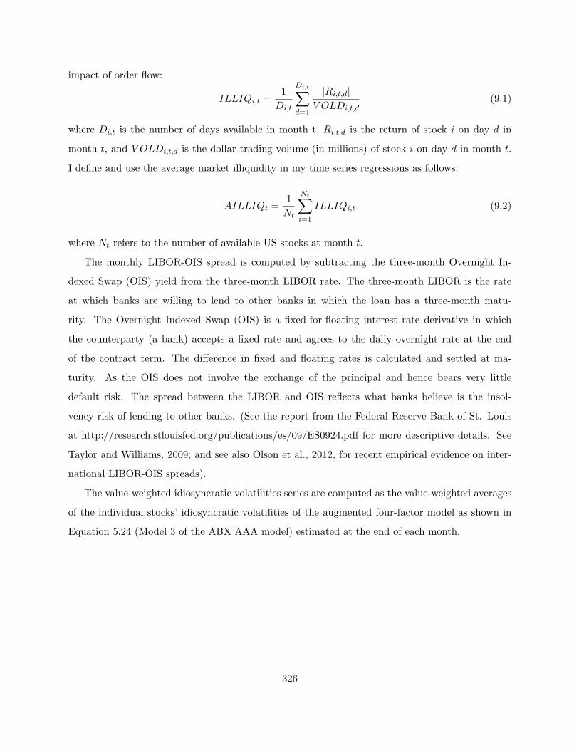
impact of order flow:
ILLIQi,t =1
Di,t
Di,t∑d=1
|Ri,t,d|V OLDi,t,d
(9.1)
where Di,t is the number of days available in month t, Ri,t,d is the return of stock i on day d in
month t, and V OLDi,t,d is the dollar trading volume (in millions) of stock i on day d in month t.
I define and use the average market illiquidity in my time series regressions as follows:
AILLIQt =1
Nt
Nt∑i=1
ILLIQi,t (9.2)
where Nt refers to the number of available US stocks at month t.
The monthly LIBOR-OIS spread is computed by subtracting the three-month Overnight In-
dexed Swap (OIS) yield from the three-month LIBOR rate. The three-month LIBOR is the rate
at which banks are willing to lend to other banks in which the loan has a three-month matu-
rity. The Overnight Indexed Swap (OIS) is a fixed-for-floating interest rate derivative in which
the counterparty (a bank) accepts a fixed rate and agrees to the daily overnight rate at the end
of the contract term. The difference in fixed and floating rates is calculated and settled at ma-
turity. As the OIS does not involve the exchange of the principal and hence bears very little
default risk. The spread between the LIBOR and OIS reflects what banks believe is the insol-
vency risk of lending to other banks. (See the report from the Federal Reserve Bank of St. Louis
at http://research.stlouisfed.org/publications/es/09/ES0924.pdf for more descriptive details. See
Taylor and Williams, 2009; and see also Olson et al., 2012, for recent empirical evidence on inter-
national LIBOR-OIS spreads).
The value-weighted idiosyncratic volatilities series are computed as the value-weighted averages
of the individual stocks’ idiosyncratic volatilities of the augmented four-factor model as shown in
Equation 5.24 (Model 3 of the ABX AAA model) estimated at the end of each month.
326
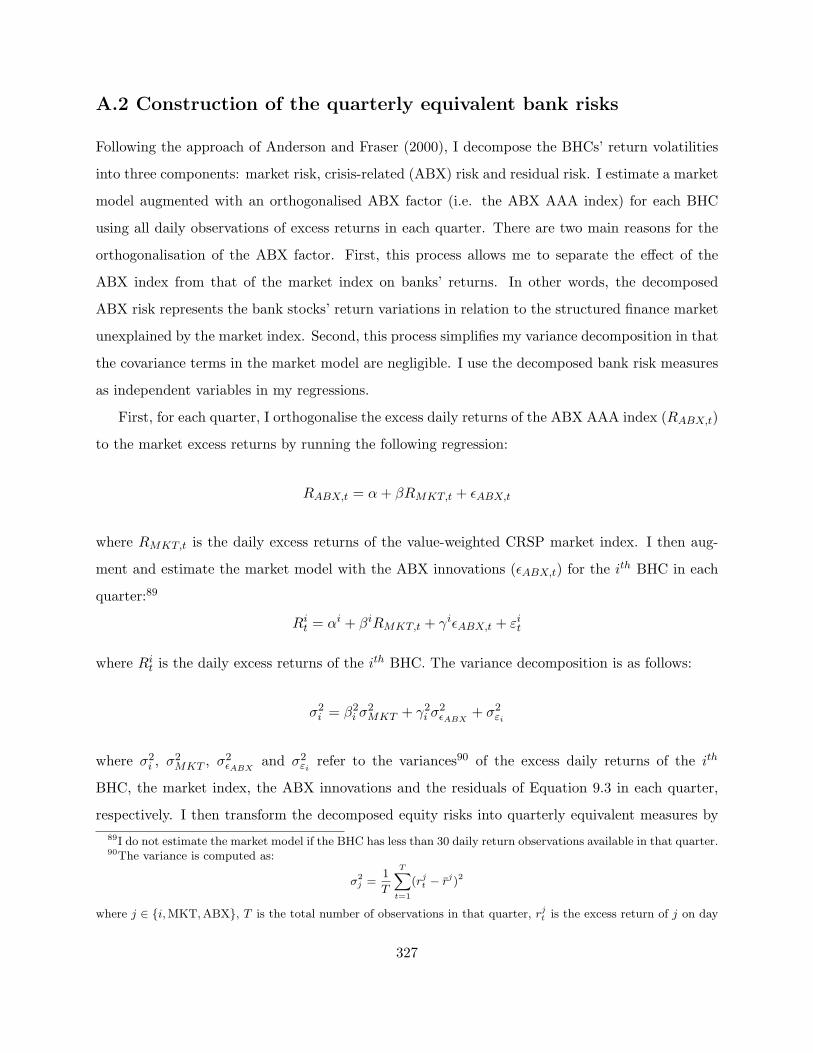
A.2 Construction of the quarterly equivalent bank risks
Following the approach of Anderson and Fraser (2000), I decompose the BHCs’ return volatilities
into three components: market risk, crisis-related (ABX) risk and residual risk. I estimate a market
model augmented with an orthogonalised ABX factor (i.e. the ABX AAA index) for each BHC
using all daily observations of excess returns in each quarter. There are two main reasons for the
orthogonalisation of the ABX factor. First, this process allows me to separate the effect of the
ABX index from that of the market index on banks’ returns. In other words, the decomposed
ABX risk represents the bank stocks’ return variations in relation to the structured finance market
unexplained by the market index. Second, this process simplifies my variance decomposition in that
the covariance terms in the market model are negligible. I use the decomposed bank risk measures
as independent variables in my regressions.
First, for each quarter, I orthogonalise the excess daily returns of the ABX AAA index (RABX,t)
to the market excess returns by running the following regression:
RABX,t = α+ βRMKT,t + ϵABX,t
where RMKT,t is the daily excess returns of the value-weighted CRSP market index. I then aug-
ment and estimate the market model with the ABX innovations (ϵABX,t) for the ith BHC in each
quarter:89
Rit = αi + βiRMKT,t + γiϵABX,t + εit
where Rit is the daily excess returns of the ith BHC. The variance decomposition is as follows:
σ2i = β2i σ2MKT + γ2i σ
2ϵABX
+ σ2εi
where σ2i , σ2MKT , σ
2ϵABX
and σ2εi refer to the variances90 of the excess daily returns of the ith
BHC, the market index, the ABX innovations and the residuals of Equation 9.3 in each quarter,
respectively. I then transform the decomposed equity risks into quarterly equivalent measures by
89I do not estimate the market model if the BHC has less than 30 daily return observations available in that quarter.90The variance is computed as:
σ2j =
1
T
T∑t=1
(rjt − rj)2
where j ∈ i,MKT,ABX, T is the total number of observations in that quarter, rjt is the excess return of j on day
327

multiplying the decomposed standard deviations by the square root of the total number of days in
each quarter, as follows:
σTOTALi = σi ×
√T
σMKTi =
√β2i σ
2MKT ×
√T
σABXi =
√γ2i σ
2ϵABX
×√T
σRESIDi = σεi ×
√T
where T is the number of daily observations in each quarter. Banks’ total, market systematic, crisis-
related (ABX), and residual risks are denoted as σTOTAL, σMKT , σABX , and σRESID respectively.
t and rj is the simple average daily excess returns of j in that quarter. The error variance of BHC i is computed as:
σ2εi =
1
T
T∑t=1
(εit − εi)2
328
Bibliography
[1] Acharya, V. V., Schnabl, P., Suarez, G., 2013. Securitization Without Risk Transfer. Journal
of Financial Economics 107(3), 515-536.
[2] Acharya, V. V., Pedersen, L. H., 2005. Asset Pricing with Liquidity Risk. Journal of Financial
Economics 77(2), 375-410.
[3] Adrian, T., Shin, H. S., 2010. The Changing Nature of Financial Intermediation and the
Financial Crisis of 2007-2009. Annual Review of Economics 2, 603-618.
[4] Allen, F., Gale, D., 2000. Financial Contagion. The Journal of Political Economy 108(1),
1-33.
[5] Amihud, Y., 2002. Illiquidity and Stock Returns: Cross-section and Time Series Effects.
Journal of Financial Markets 5(1), 31-56.
[6] Anand, A., Irvine, P., Puckett, A., Venkataraman, K., 2013. Institutional Trading and Stock
Resiliency: Evidence from the 2007-2009 Financial Crisis. Journal of Financial Economics
108, 773-797.
[7] Anderson, R. C., Fraser, D. R., 2000. Corporate Control, Bank Risk Taking, and the Health
of the Banking Industry. Journal of Banking and Finance 24(8), 13831398.
[8] Anderson, T., Hsiao, C., 1981. Estimation of Dynamic Models with Error Componenets.
Journal of the American Statistical Association 76(375), 598-606.
[9] Ang, A., Hodrick, R., Xing, Y., Zhang, X., 2006. The Cross-section of Volatility and Expected
Returns. Journal of Finance 61, 259-299.
329
[10] Ang, A., Hodrick, R., Xing. Y., Zhang, X., 2009. High Idiosyncratic Volatility and Low
Returns: International and Further U.S. Evidence. Journal of Financial Economics 91(1),
1-23.
[11] Arellano, M., Bond, S., 1991. Some Tests of Specification for Panel Data: Monte Carlo
Evidence and An Application to Employment Equations. The Review of Economic Studies
58(2), 277-297.
[12] Baig, T., Goldfajn, I., 1999. Financial Market Contagion in the Asian Crisis. IMF Staff Papers
46, 167-195.
[13] Banz, R., 1981. The Relation Between Return and Market Value of Common Stocks. Journal
of Financial Economics 9, 3-18.
[14] Barber, B. M., Lyon, J. D., 1997. Firm Size, Book-to-Market Ratio and Security Returns: A
Holdout Sample of Financial Firms. Journal of Finance 52(2), 875-883.
[15] Barber, D. M., Odean, T., 2000. Trading Is Hazardous to Your Wealth: The Common Stock
Investment Performance of Individual Investors. Journal of Finance 55, 773-806.
[16] Basu, S. 1975. The Information Content of Price-Earnings Ratios. Financial Management 4,
53-64.
[17] Basu, S., 1983. The Relationship Between Earnings’ Yield, Market Value and Return for
NYSE Common Stocks: Further Evidence. Journal of Financial Economics 12, 129-156.
[18] Baur, D. G., Lucey, B. M., 2009. Flights and Contagion - An Empirical Analysis of Stock-
Bond Correlations. Journal of Financial Stability 5(4), 339-352.
[19] Baur, D. G., McDermott, T. K., 2010. Is Gold a Safe Haven? International Evidence. Journal
of Banking and Finance 34(8), 1886-1898.
[20] BBC News. Timeline: Sub-prime losses. 2008. Available at:
http://news.bbc.co.uk/1/hi/business/7096845.stm [Accessed: September 2012].
[21] Bekaert, G., Harvey, C. R., Ng, A., 2005. Market Integration and Contagion. Journal of
Business 27, 39-69.
330

[22] Bekaert, G., Ehrmann, M., Fratzscher, M., Mehl, A. J., 2011. Global Crises and Equity
Market Contagion. National Bureau of Economics Research Working Paper Series, no. 17121,
Jun 2011.
[23] Beltratti, A., Stulz, R. M., 2012. The Credit Crisis Around the Globe: Why Did Some Banks
Perform Better? Journal of Financial Ecomomics 105, 1-17.
[24] Ben-David, I., Franzoni, F., Moussawi, R., 2012. Hedge Fund Stock Trading in the Financial
Crisis of 20072009. The Review of Financial Studies 25(1), 1-54.
[25] Benmelech, E., Dlugosz, J., 2009. The Credit Rating Crisis. Working Paper, Harvard Univer-
sity.
[26] Berger, A. N., Bouwman, C. H. S., 2012. How Does Capital Affect Bank Performance During
Financial Crises? Journal of Financial Economics, Forthcoming.
[27] Bernard, V., Thomas, J., 1990. Evidence that Stock Prices Do Not Fully Reflect the Impli-
cations of Current Earnings for Future Earnings. Journal of Accounting and Economics 13,
305-341.
[28] Bessler, W., Drobetz, W., Erdmann, T., Zimmermann, H., 2007. Predictability in the Cross-
section of European Bank Stock Returns. WWZ Working Paper 21/07.
[29] Bhat, V. N., 1996. Banks and Income Smoothing: An Empirical Analysis. Applied Financial
Economics 6(6), 505-510.
[30] Bikhchandani, S., Hirshleifer, D., Welch, I., 1998. Learning From the Behavior of Others:
Conformity, Fads, and Informational Cascades. Journal of Economic Perspectives 12(3), 151-
170.
[31] Black, F., Jensen, M. C., Scholes, M., 1972. The capital asset pricing model: some empirical
tests. In: Jensen, M.C. (ed.), Studies in the Theory of Capital Markets, pp.79121. Praeger,
New York (1972)
[32] Bollerslev, T., 1990. Modeling the Coherence in Short-run Nominal Exchange Rates: A Mul-
tivariate Generalized ARCH Model. Review of Economics and Statistics 72(3), 498-505.
331
[33] Bollerslev, T., Engle, R. F., Wooldridge, J. M., 1988. A Capital-Asset Pricing Model with
Time-varying Covariances. Journal of Political Economy 96(1), 116-131.
[34] Bouaziz, M. C., Selmi, N., Boujelbene, Y., 2012. Contagion Effect of The Subprime Financial
Crisis: Evidence of DCC Multivariate GARCH Models. European Journal of Economics,
Finance and Administrative Sciences 44, 66-76.
[35] Boyer, B. H., Gibson, M. S., Loretan, M., 1999. Pitfalls in Tests for Changes in Correlations.
Federal Reserve Board International Finance Division, Working Paper 597R.
[36] Boyson, N. M., Stahel, C. W., Stulz, R. M., 2010. Hedge Fund Contagion and Liquidity
Shocks. Journal of Finance 65(5), 1789-1816.
[37] Brown, K. C., Harlow, W. V., Smith, D. J., 1994. An Empirical Analysis of Interest Rate
Swap Spreads. Journal of Fixed Income 3(4), 61-78.
[38] Brunnermeier, M. K., 2009. Deciphering the Liquidity and Credit Crunch. Journal of Eco-
nomic Perspectives 23(1), 77-100.
[39] Brunnermeier, M. K., Pedersen, L. H., 2009. Market Liquidity and Funding Liquidity. Review
of Financial Studies 22(6), 2201-2238.
[40] Bryant, J., 1980. A Model of Reserves, Bank Runs, and Deposit Insurance. Journal of Banking
and Finance 4(4), 335-344.
[41] Calvo, G., 1998. Understanding the Russian Virus (with Special Reference to Latin America).
University of Maryland, Department of Economics, College Park, Md. Processed.
[42] Calvo, G., Mendoza, E. G., 2000. Rational Contagion and the Globalization of Securities
Markets. Journal of International Economics, 51(1), 79-113.
[43] Calvo, S., Reinhart, C., 1995. Capital Inows to Latin America: Is there Evidence Of Contagion
Effects? WorldBank and International Monetary Fund, unpublished.
[44] Cameron, A. C., Gelbach, J. B., Miller, D. L., 2011. Robust Inference With Multiway Clus-
tering. Journal of Business & Economic Statistics 29, 238-249.
332
[45] Campbell, J. Y., Lettau, M., Malkiel, B. G., Xu, Y., 2001. Have Individual Stocks Become
More Volatile? An Empirical Exploration of Idiosyncratic Risk. Journal of Finance 56, 1-43.
[46] Campbell, J. Y., Shiller, R. J., 1988. The Dividend-Price Ratio and Expectations of Future
Dividends and Discount Factors. Review of Financial Studies 1, 195-228.
[47] Caramazza, F., Ricci, L., Salgado, R., 2000. Trade and Financial Contagion in Currency
Crises. IMF Working Papers 00/55, International Monetary Fund.
[48] Caramazza, F., Ricci, L., Salgado, R., 2004. International Financial Contagion in Currency
Crises. Journal of International Money and Finance 23(1), 5170.
[49] Carhart, M. M., 1997. On Persistence in Mutual Fund Performance. Journal of Finance 52(1),
57-82.
[50] Caruana, J., Kodres, L., 2008. Liquidity in Global Markets. Financial Stability Review, Special
Issue on Liquidity, Banque de France, 11(Dec), 65-74.
[51] Celent Consultant. 2005. Report on Collateralized Debt Obligations Market. Available
at: http://www.celent.com/reports/collateralized-debt-obligations-market [Accessed in: May
2010]
[52] Chen, N. F., Roll, R., Ross, S. A., 1986. Economic Forces and the Stock Market. Journal of
Business 59, 383-403.
[53] Chiang, T. C., Jeon, B. N., Li, H., 2007. Dynamic Correlation Analysis of Financial Con-
tagion: Evidence from Asian markets. Journal of International Money and Finance 26(7),
1206-1228.
[54] Cho, J. H., Parhizgari, A. M., 2008. East Asian Financial Contagion Under DCC GARCH.
International Journal of Banking and Finance 6(1), 17-30.
[55] Chordia, T., Subrahmanyam, A., Anshuman, V. R., 2001. Trading Activity and Expected
Stock Returns. Journal of Financial Economics 59(Jan), 3-32.
[56] Christie, A. A., 1982. The Stochastic Behavior of Common Stock Variances: Value, Leverage
and Interest Rate Effects. Journal of Financial Ecomomics 10(4), 407-432.
333
[57] Claessens, S., Kose, M. A., Terrones, M. E., 2010. The Global Financial Crisis: How Similar?
How Different? How Costly? Journal of Asian Economics 21(3), 247-264.
[58] Cochrane, J. H., 2000. Asset Pricing. Princeton University Press, Princeton, New Jersey.
[59] Comerton-Forde, C., Hendershott, T., Jones, C. M., Moulton, P. C., Seasholes, M. S., 2010.
Time Variation in Liquidity: The Role of Market-Maker Inventories and Revenues. Journal
of Finance 65, 295-331.
[60] Connolly, R., Wang, F. A., 2003. International Equity Market Comovements: Economic
Fundamentals or Contagion? Pacific-Basin Finance Journal 11(1), 23-43.
[61] Cooper, M. J., Jackson, W. E., Patterson, G. A., 2003. Evidence of Predictability in the
Cross-section of Bank Stock Returns. Journal of Banking and Finance 27(5), 817-850.
[62] Cornett, M. M., McNutt, J. J., Strahan, P. E., Tehranian, H., 2011. Liquidity Risk Man-
agement and Credit Supply in the Financial Crisis. Journal of Financial Economics 101,
297-312.
[63] Corsetti, G., Pericoli, M., Sbracia, M., 2001. Correlation Analysis of Financial Contagion:
What One Should Know Before Running a Test. Unpublished Working Paper. University of
Rome III Working Paper.
[64] Corsetti, G., Pericoli, M., Sbracia, M., 2005. “Some Contagion, Some Interdependence”: More
Pitfalls in Tests of Financial Contagion. Journal of International Money and Finance 24(8),
1177-1199.
[65] Coval, J. D., Stafford, E, 2007. Asset Fire Sales (and Purchases) in Equity Markets. Journal
of Financial Economics 86, 479-512.
[66] Cox, J, Glapa, L., 2009. Credit Crisis Timeline. The University of IOWA Center for
International Finance & Development.
Available at: http://ebook.law.uiowa.edu/ebook/sites/default/files/Financial Crisis Timeline.pdf
[Accessed in September 2012].
[67] Daniel, K., Hirshleifer, D., Subrahmanyam, A., 1998. Investor Psychology and Investor Se-
curity Market Under- and Overreactions. Journal of Finance 53, 18391886.
334
[68] Demsetz, R., Saidenberg, M., Strahan, P., 1997. Agency Problems and Risk Taking at Banks.
Working paper, Federal Reserve Bank of New York.
[69] Diamond, D. V., Dybvig, P., 1983. Bank Runs, Deposit Insurance, and Liquidity. Journal of
Political Economy, 91(3), 401-419.
[70] Diamond, D. W., Rajan, R.G., 2000. A theory of Bank Capital. Journal of Finance 55,
2431-2465.
[71] Dick-Nielsen, J., Feldhutter, P., Lando, D., 2012. Corporate Bond Liquidity Before and After
the Onset of the Subprime Crisis. Journal of Financial Economics 103(3), 471-492.
[72] Dimson, E., 1979. Risk measurement when shares are subject to infrequent trading. Journal
of Financial Economics, 7, 197-226.
[73] Dooley, M., Hutchison, M., 2009. Transmission of the U.S. Subprime Crisis to Emerging Mar-
kets: Evidence on the Decoupling-Recoupling Hypothesis. Journal of International Money
and Finance 28(8), 1331-1349.
[74] Dornbusch, R., Park, Y. C., Claessens, S., 2000. Contagion: Understanding How It Spreads.
The World Bank Research Observer 15(2), 177-197.
[75] Drehmann, M., Nikolaou, K., 2012. Funding Liquidity Risk: Definition and Measurement.
Journal of Banking and Finance 37(7), 21732182.
[76] Dungey, M., Martin, V.L., 2001. Contagion Across Financial Markets: An Empirical Assess-
ment. New York Stock Exchange Conference Paper, February, 1617.
[77] Dungey, M., Martin, V.L., 2004. A Multifactor Model of Exchange Rates With Unanticipated
Shocks: Measuring Contagion in the East Asian Currency Crisis. Journal of Emerging Market
Finance 3(3), 305-330.
[78] Dungey, M., Zhumabekova, D., 2001. Testing for Contagion Using Correlations: Some Words
of Caution. Pacific Basin Working Paper Series 01-09, Federal Reserve Bank of San Francisco.
[79] Dungey, M., Fry, R., Gonzalez-Hermosillo, B., Martin, V. L., 2002a. International Contagion
Effects from the Russian Crisis and the LTCM Near-Collapse. IMF Working Paper 02/74.
335
[80] Dungey, M., Fry, R., Gonzalez-Hermosillo, B., Martin, V. L., 2002b. The Transmission of
Contagion in Developed and Developing International Bond Markets, in Committee on the
Global Financial System (ed), Risk Measurment and Systemic Risk, Proceedings of the Third
Joint Central Bank Research Conference, 6174.
[81] Dungey, M., Fry, R., Gonzalez-Hermosillo, B., Martin, V., 2005. Empirical Modeling of Con-
tagion: A Review of Methodologies. Quantitative Finance 5(1), 9-24.
[82] Dungey, M., Fry, R., Gonzalez-Hermosillo, B., Martin, V., 2006. Contagion in International
Bond Markets During the Russian and LTCM Crises. Journal of Financial Stability 2(1),
1-27.
[83] Edmans, A., 2011. Does the Stock Market Fully Value Intangibles? Employee Satisfaction
and Equity Prices. Journal of Financial Economics 101, 621-640.
[84] Edmonds, T., Jarrett, T., Woodhouse, J., 2010. The Credit Crisis: A Timeline. Available at:
www.parliament.uk/briefing-papers/sn04991.pdf [Accessed in: Oct 2012].
[85] Edwards, S., 1998. Interest Rate Volatility, Contagion And Convergence: An Empirical In-
vestigation Of The Cases Of Argentina, Chile And Mexico. Journal of Applied Economics 1,
55-86.
[86] Eichengreen, B., 2008. Ten Questions About the Subprime Crisis. Banque de France: Finan-
cial Stability Review: Special Issue on Liquidity, Banque de France, 11(Feb), 19-28.
[87] Eichengreen, B., Rose, A. K., Wyplosz, C., 1996. Contagious Currency Crises: First Tests.
Scandinavian Journal of Economics 98, 463-484.
[88] Eichengreen, B., Mody, A., Nedeljkovic, M., Sarno, L., 2009. How the Subprime Crisis Went
Global: Evidence from Bank Credit Default Swap Spreads. Journal of International Money
and Finance 31(5), 12991318.
[89] Elyasiani, E., Mansur, I., 1998. Sensitivity of the Bank Stock Returns Distribution to Changes
in the Level and Volatilities of Interest Rate: A GARCH-M Model. Journal of Banking and
Finance, 22(5), 535-563.
336
[90] Enders, W., 2003. RATS Programming Language. Instruction book by Estima. Available at:
http://www.estima.com/enders [Accessed in May 2012].
[91] Engle, R., 2002. Dynamic Conditional Correlation: A Simple Class of Multivariate Gener-
alized Autoregressive Conditional Heteroskedasticity Models. Journal of Business and Eco-
nomic Statistics 20(3) 339-50.
[92] Engle, R. F., Ito, T., Lin, W. L., 1990. Meteor Showers or Heat Waves? Heteroskedastic
Intra-Daily Volatility in the Foreign Exchange Market. Econometrica 58(3), 525-542.
[93] European Central Bank, 2012. Timeline of the Financial Crisis.
Available at: http://www.ecb.int/ecb/html/crisis.en.html [Accessed in September 2012]
[94] Evans, K. P., 2011. Intraday Jumps and US Macroeconomic News Announcements. Journal
of Banking and Finance 35(10), 2511-2527.
[95] Fahlenbrach, R., Prilmeier, R., Stulz, R. M., 2012. This Time Is the Same: Using Bank
Performance in 1998 to Explain Bank Performance during the Recent Financial Crisis. Journal
of Finance 67(6), 2139-2185.
[96] Fahlenbrach, R., Stulz, R. M., 2011. Bank CEO Incentives and the Credit Crisis. Journal of
Financial Economics 99, 11-26.
[97] Falkenstein, E. G., 1996. Preferences for Stock Characteristics As Revealed by Mutual Fund
Portfolio Holdings. Journal of Finance 51, 111-135.
[98] Fama, E. F., French, K. R., 1988. Dividend Yields and Expected Stock Returns. Journal of
Financial Economics 22, 3-25.
[99] Fama, E., French, K. R., 1992. The Cross-section of Expected Stock Returns. Journal of
Finance 48, 427-465.
[100] Fama, E. F., French, K. R., 1993. Common Risk Factors in the Returns on Stocks and Bonds.
Journal of Financial Economics 33(1), 3-56.
[101] Fama, E. F., Macbeth, J. D., 1973. Risk, Return, and Equilibrium: Empirical Tests. Journal
of Political Economy 81(3), 607-636.
337
[102] Favero, C. A., Giavazzi, F., 2002. Is the International Propagation of Financial Shocks Non-
Linear? Evidence from the ERM. Journal of International Economics 57(1), 231-246.
[103] Fender, I., Hordahl, P., 2008. A Cautious Return of Risk Tolerance. BIS Quarterly Review
June, 1-16.
[104] Fender, I., Scheicher, M., 2009. The Pricing of Subprime Mortgage Risk in Good Times and
Bad: Evidence From the ABX.HE Indices. Applied Financial Economics, Taylor and Francis
Journals 19(24), 1925-1945.
[105] Flannery, J., Kwan, S. H., Nimalendran M.,2004. Market Evidence on the Opaqueness of
Banking Firms’ Assets. Journal of Financial Economics 71(3), 419-460.
[106] Flannery, J., Kwan, S. H., Nimalendran M., 2013. The 2007-2009 Financial Crisis and Bank
Opaqueness. Journal of Financial Intermediation 22(1), 55-84.
[107] Fonseca, A. R., Gonzalez, F., 2008. Cross-country Determinants of Bank Income Smoothing
by Managing Loan Loss Provisions. Journal of Banking and Finance 32(2), 217-228.
[108] Forbes, K. J., 2004. The Asian Flu and Russian Virus: the International Transmission of
Crises in Firm-level Data. Journal of International Economics 63(1), 59-92.
[109] Forbes, K. J., Rigobon, R., 2002. No Contagion, Only Interdependence: Measuring Stock
Market Comovements. The Journal of Finance 57(5), 2223-2261.
[110] Frank, N., Gonzalez-Hermosillo, B., Hesse, H., 2008. Transmission of Liquidity Shocks: Evi-
dence from the 2007 Subprime Crisis. IMF Working Paper, August 2008.
[111] French, K., Schwert, G., Stambaugh, R., 1987. Expected Stock Returns and Volatility. Journal
of Financial Economics 19, 3-29.
[112] French, K. R., et al. 2010. The Squam Lake Report. Princeton University Press: Princeton,
NJ.
[113] Fu, F., 2009. Idiosyncratic Risk and the Cross-section of Expected Stock Returns. Journal of
Financial Economics 91(1), 24-37.
338
[114] Gandhi, P., Lustig, H., 2011. Size Anomalies in U.S. Bank Stock Returns: A Fiscal Explana-
tion, Working paper, UCLA.
[115] Gatev, E., Strahan, P. E., 2006. Banks’ Advantage in Hedging Liquidity Risk: Theory and
Evidence from the Commercial Paper Market. The Journal of Finance 61(2), 867-892.
[116] Gervais, S., Kaniel, R., Mingelgrin, D. H., 2001. The High-volume Return Premium. Journal
of Finance 56, 877-919.
[117] Goeij, P., Marquering, W., 2004. Modelling the Conditional Covariance Between Stock and
Bond Returns: a Multivariate GARCH Approach. Journal of Financial Econometrics 2(4),
531-564.
[118] Gorton, G. B., 2009. The Subprime Panic. European Financial Management 15, 10-46.
[119] Gorton, G. B., Metrick, A., 2012. Securitized Banking and the Run on Repo. Journal of
Financial Economics 104(3), 425-451.
[120] Gorton, G. B., Pennacchi, G., 1990. Financial-intermediaries and Liquidity Creation. Journal
of Finance 45(1), 49-71.
[121] Goyal, A., Santa-Clara, P., 2003. Idiosyncratic Risk Matters! Journal of Finance 58, 975-
1008.
[122] Grammatikos, T., Saunders, A., Swary, I., 1986. Return and Risks of US Bank Foreign
Currency Activities. Journal of Finance 41, 671-682.
[123] Grinblatt, M., Titman, S., Werners, R., 1995. Momentum Investment Strategies, Portfolio
Performance, and Herding: A Study of Mutual Fund Behavior. American Economic Review
85, 1088-1105.
[124] Grinblatt, M., 2001. An Analytic Solution for Interest Rate Swap Spreads. International
Review of Finance 2(3), 113-149.
[125] Guesmi, K., Kaabia, O., Kazi, I., 2013. Does Shift Contagion Exist Between OECD Stock
Markets During the Financial Crisis? Journal of Applied Business Research 29(2), 469-484.
339
[126] Gunther, J. W., Moore, R. R., 2003. Loss Underreporting and the Auditing Role of Bank
Exams. Journal of Financial Intermediation 12(2), 153-177.
[127] Hamao, Y., Masulis, R., Ng, V., 1990. Correlations in Price Changes and Volatility Across
International Stock Markets. Review of Financial Studies 3(2), 281-307.
[128] Haq, M., Heaney, R., 2012. Factors determining European bank risk. Journal of International
Financial Markets, Institutions & Money 22, 696-718.
[129] Hardy, D. C., Pazarbasioglu, C., 1998. Leading Indicators of Banking Crises: Was Asia
Different? IMF Working Paper, 91.
[130] Harris, M., Raviv, A., 1991. The Theory of Capital Structure. Journal of Finance 46(1),
297-355.
[131] Hui, C. H., Lam, L., 2008. What Drives Hong Kong Dollar Swap Spreads: Credit or Liquidity?
Working paper, Hong Kong Monetary Authority.
[132] Iannotta, G. O., 2006. Testing for Opaqueness in the European Banking Industry: Evidence
From Bond Credit Ratings. Journal of Financial Services Research 30(3), 287-309.
[133] In, F., 2007. Volatility Spillovers Across International Swap Markets: The US, Japan, and
the UK. Journal of International Money and Finance 26(3), 329-341.
[134] Irvine, P. J., Pontiff, J., 2008. Idiosyncratic Return Volatility, Cash Flows, and Product
Market Competition. Review of Financial Studies 22(3), 1149-1177.
[135] Jaffee, D. W., 2008. The U.S. Subprime Mortgage Crisis: Issues Raised and Lessons Learned.
Working Paper No. 28, Commission on Growth and Development.
[136] Jegadeesh, N., Titman, S., 1993. Returns to Buying Winners and Selling Losers: Implications
for Stock Market Efficiency. Journal of Finance 48, 65-92.
[137] Jegadeesh, N., Titman, S., 2001. Profitability of Momentum Strategies: An Evaluation of
Alternative Explanations. Journal of Finance 56, 699-720.
[138] Jones, C. M., Kaul, G., Lipson, M. L., 1994. Information, Trading and Volatility. Journal of
Financial Economics 36(1), 127-154
340
[139] Jones, J. S., Lee, W. Y., Yeager, T. J., 2013. Valuation and Systematic Risk Consequences
of Bank Opacity. Journal of Banking and Finance 37(3), 693-706.
[140] Jotikasthira, C., Lundblad, C., Ramadorai, T., 2012. Asset Fire Sales and Purchases and the
International Transmission of Funding Shocks. Journal of Finance 67, 2015-2050.
[141] Kaminsky, G. L., 1999. Currency and Banking Crises: The Early Warnings of Distress. IMF
Working Paper, No. 99/178, pp. 1-38.
[142] Kaminsky, G. L., Reinhart, C. M., 2000. On Crises, Contagion, and Confusion. Journal of
International Economics 51(1), 145-168.
[143] Kaminsky, G. L., Reinhart, C. M., 2001. Financial Markets in Times of Stress. NBERWorking
Paper no. 8569.
[144] Kaminsky, G. L., Reinhart, C. M., Vgh, C. A., 2003. The Unholy Trinity of Financial Con-
tagion. The Journal of Economic Perspectives, 17(4), 51-74.
[145] Kaniel, R., Ozoguz, A., Starks, L., 2012. The High Volume Return Premium: Cross Country
Evidence. Journal of Financial Economics 103(2), 255279.
[146] Karpoff, J. M., 1987. The Relation Between Price Changes and Trading Volume: A Survey.
The Journal of Financial and Quantitative Analysis 22(1), 109-126.
[147] Keeley, M., 1990. Deposit Insurance, Risk, and Market Power in Banking. American Economic
Review 80(5), 1184-1200.
[148] Kenc, T., Dibooglu, S., 2010. The 20072009 Financial Crisis, Global Imbalances and Capital
Flows: Implications for Reform. Economic Systems 34(1), 3-21.
[149] King, M., Wadhwani, S., 1990. Transmission of Volatility Between Stock Markets. Review of
Financial Markets 3(1), 5-33.
[150] Kiyotaki, N., Moore, J., 2002. Evil is the Root of All Money. American Economic Review:
Papers and Proceedings 92, 62-66.
[151] Kodres, L., Pritsker, M., 2002. A Rational Expectations Model of Financial Contagion. Jour-
nal of Finance 57(2), 769-800.
341
[152] Konishi, M., Yasuda, Y., 2004. Factors Affecting Bank Risk Taking: Evidence from Japan.
Journal of Banking and Finance 28(1), 215-232.
[153] Lamont, O., 1998. Earnings and Expected Returns. Journal of Finance 53, 1563-1587.
[154] Lewellen, J., Nagel, S., 2006. The Conditional CAPM Does Not Explain Asset-Pricing
Anomalies. Journal of Financial Economics 82, 289-314.
[155] Li, L., 2003. Macroeconomic Factors and the Correlation of Stock and Bond Return. Yale
School of Management Working Papers, November.
[156] Lindsey, L. B., 2007. Fear and Greed: Why the American Housing Credit Crisis is Worse
Than You Think. International Economy 21(2), 22-55.
[157] Liu, J., Longstaff, F. A., Mandell, R. E., 2006. The Market Price of Risk in Interest Rate
Swaps: The Roles of Default and Liquidity Risks. Journal of Business 79(5), 2337-2360.
[158] Lo, A., MacKinlay, A. C., 1990. When are Contrarian Profits Due to Stock Market Overre-
action? Review of Financial Studies 3, 175-205.
[159] Longstaff, F. A., 2004. The Flight-to-Liquidity Premium in U.S. Treasury Bond Prices. Jour-
nal of Business 77(3), 511-526.
[160] Longstaff, F. A., 2010. The Subprime Credit Crisis and Contagion in Financial Markets.
Journal of Financial Economics 97(3), 436-450.
[161] Loretan, M., English, W., 2000. Evaluating “Correlation Breakdown” During Periods of Mar-
ket Volatility. International Finance Discussion Paper No. 658, 2000 (Board of Governors of
the Federal Reserve System).
[162] Mahlmann, T., 2013. Hedge Funds, CDOs and the Financial Crisis: An Empirical Investiga-
tion of the Magnetar Trade. Journal of Banking and Finance 37(2), 537-548.
[163] Marcal, E. F., Pereira, P. L. V., Martin, D. M. L., Nakamura, W. T., 2011. Evaluation of
Contagion or Interdependence in the Financial Crises of Asia and Latin America, Considering
the Macroeconomic Fundamentals. Applied Economics 43(19), 2365-2379.
342
[164] McSweeney, B. 2009. The Roles of Financial Asset Market Failure Denial and the Economic
Crisis: Reflections on Accounting and Financial Theories and Practices. Accounting, Organi-
zations and Society 34(6-7), 835848.
[165] Meeker, L. G., Gray, L., 1987. A Note on Non-Performing Loans As An Indicator of Asset
Quality. Journal of Banking and Finance 11(1), 161-168.
[166] Merrill, C. B., Nadauld, T. D., Stulz, R. M., Sherlund, S., 2012. Did Capital Requirements
and Fair Value Accounting Spark Fire Sales in Distressed Mortgage-Backed Securities? NBER
Working Paper 18270, August.
[167] Merton, R., 1987. A Simple Model of Capital Market Equilibrium with Incomplete Informa-
tion. Journal of Finance 42, 483-510.
[168] Milunovich, G., Tan, A., 2013. Testing for Contagion in US Industry Portfolios - a Four-Factor
Pricing Approach. Applied Financial Economics 23, 15-26.
[169] Mizen, P., 2008. The Credit Crunch of 2007-2008: A Discussion of the Background, Market
Reactions, and Policy Responses. Federal Reserve Bank of St. Louis Review, 90(5), 531-567.
[170] Morgan, D., 2002. Rating Banks: Risk and Uncertainty in An Opaque Industry. American
Economic Review 92(4), 874-888.
[171] Nagayasu, J., 2001. Currency Crisis and Contagion: Evidence from Exchange Rates and
Sectoral Stock Indices of the Philippines and Thailand. Journal of Asian Economics 12(4),
529-546.
[172] Naoui, K., Liouane, L. Brahim, S., 2010. A Dynamic Conditional Correlation Analysis of
Financial Contagion: The Case of the Subprime Credit Crisis. International Journal of Eoc-
nomics and Finance 2(3), 85-96.
[173] National Bureau of Economic Research (NBER) Summer Institute, 2008. Recent De-
velopments in Structural VAR Modeling. Available at: www.nber.org/WNE/slides7-14-
08/Lecture7.pdf [Accessed in May 2012].
[174] Newey, W. K., West, K. D., 1987. A Simple, Positive Semi-definite Heteroskedasticity and
Autocorrelation Consistent Covariance Matrix. Econometrica 55(3), 703-708.
343
[175] Ng, A., 2000. Volatility Spillover Effects from Japan and the U.S. to the Pacific-Basin. Journal
of International Money and Finance 19(2), 207-233.
[176] Noeth, B., Sengupta, R., 2010. Flight To Safety and US Treasury Securities. The Regional
Economist July, 1-2.
[177] Olson, E., Miller, S., Wohar, M. E., 2012. “Black Swans” Before the “Black Swan” Evidence
From International LIBOR-OIS Spreads. Journal of International Money and Finance 31(6),
1339-1357.
[178] Partnoy, F., 2009. Overdependence on Credit Ratings Was a Primary Cause of the Crisis. In:
Proceedings of the 2008 International Banking Conference: ‘The First Credit Market Turmoil
of the 21st Century’, World Scientic Publishers.
[179] Pastor, L., Veronesi, P., 2003. Stock Valuation and Learning about Profitability. Journal of
Finance 58(5), 1749-1790.
[180] Pathan, S., 2009. Strong Boards, CEO Power and Bank Risk-taking. Journal of Banking and
Finance 33(7), 1340-1350.
[181] Pericoli, M., Sbracia, M., 2003. A Primer on Financial Contagion. Journal of Economic
Surveys 17(4), 571-608.
[182] Pesaran, M. H., Pick, A., 2007. Econometric Issues in the Analysis of Contagion. Journal of
Economic Dynamics and Control 31(4), 1245-1277.
[183] Petkova, R., 2006. Do the Fama-French Factors Proxy for Innovations in Predictive Variables?.
Journal of Finance 61(2), 581-612.
[184] Phillips C. B., Yu, J., 2011. Dating the Timeline of Financial Bubbles During the Subprime
Crisis. Quantitative Economics, 2(3), 455-491.
[185] Rajgopal, S., Venkatachalam, M., 2011. Financial Reporting Quality and Idiosyncratic Return
Volatility. Journal of Accounting and Economics 51(1-2), 1-20.
[186] Reinhart, C. M., Rogoff, K. S., 2008. Is the 2007 U.S. Subprime Crisis So Different? An
International Historical Comparison. American Economic Review 98(2), 339-344.
344
[187] Reuters, 2008. Timeline: The credit crunch of 2007/2008. Available at:
http://www.reuters.com/article/2008/08/05/us-crunch-timeline-idUSL155564520080805
[Accessed in: September 2012].
[188] Richardson, S., 2006. Over-investment of Free Cash Flow. Review of Accounting Studies 11(2-
3), 159-189.
[189] Rogers, K., Sinkey Jr., J. F., 1999. An Analysis of Nontraditional Activities at US Commercial
Banks. Review of Financial Economics 8, 25-39.
[190] Schwert, G. W., 1989. Why Does Stock Market Volatility Change Over Time? Journal of
Finance 44(5), 1115-1153.
[191] Securities Industry and Financial Markets Association, 2010. SIFMA Report. Available at:
http://www.sifma.org/research/reports.aspx [Accessed in: September 2012]
[192] Sengupta R., Emmons W. R., 2007. What is Subprime Lending? Monetary Trends, Federal
Reserve Bank of St. Louis, issue Jun.
[193] Shleifer, A., Vishny, R., 1992. Liquidation Values and Debt Capacity: A Market Equilibrium
Approach. Journal of Finance 47, 1343-1366.
[194] Shleifer, A., Vishny, R., 1997. The Limits of Arbitrage. Journal of Finance 52(1), 35-55.
[195] Shleifer, A., Vishny, R., 2011. Fire Sales in Finance and Macroeconomics. Journal of Economic
Perspectives 25, 29-48.
[196] Shumway, T., 1997. The Delisting Bias in CRSP Data. The Journal of Finance 52, 327-340.
[197] Sims, C. A., 1980. Macroeconomics and Reality. Econometrica 48(1), 1-48.
[198] Stiroh, K. J., 2006. New Evidence on the Determinants of Bank Risk. Journal of Financial
Services Research 30, 237-263.
[199] Stock, J. H., Watson, M. W., 2001. Vector Autoregressions. Journal of Economic Perspectives
15(4), 101-115.
345
[200] Swan, P. L., 2009. The Political Economy of the Subprime Crisis: Why Subprime Was So
Attractive to Its Creators. European Journal of Political Economy 25(1), 124-132.
[201] Taylor, J. B., Williams, J. C., 2009. A Black Swan in the Money Market. American Economic
Journal: Macroeconomics 1, 58-83.
[202] Thakor, A.V., 1987. Discussion. Journal of Finance 42, 661-663.
[203] Thompson, S. B., 2011. Simple Formulas for Standard Errors that Cluster by Both Firm and
Time. Journal of Financial Economics 99, 1-10.
[204] Titman, S., Wei, K. C. J., Xie, F., 2004. Capital Investments and Stock Returns. Journal of
Financial and Quantitative Analysis 39(4), 677-700.
[205] Udell, G., 2009. Wall Street, Main Street, and A Credit Crunch: Thoughts on the Current
Financial Crisis. Business Horizons 52(2), 117-125.
[206] Vassalou, M., Xing, Y., 2004. Default Risk in Equity Returns. The Journal of Finance 59(2),
831-868.
[207] Vuolteenaho, T., 2002. What Drives Firm-Level Stock Returns? Journal of Finance 57,
233-264.
[208] Wahlen, J., 1994. The Nature of Information in Commercial Bank Loan-Loss Disclosures.
Accounting Review 69(3), 455-477.
[209] Weaver, K., 2008. The Sub-prime Mortgage Crisis: A Synopsis. Global Securitisation and
Structured Finance, Deutsche Bank.
[210] Wei, S. X., Zhang, C., 2006. Why did individual stocks become more volatile? The Journal
of Business 79, 259-292.
[211] Xu, Y., Malkiel, B. G., 2003. Investigating the Behavior of Idiosyncratic Volatility. Journal
of Business 76, 613-645.
[212] Zarutskie, R., 2013. Competition, Financial Innovation and Commercial Bank Loan Portfo-
lios. Journal of Financial Intermediation 22, 373-396.
346