Financial contagion in the BRIC countries during the 2007 ... · example, Baig and Goldfajn (1999) by using the correlation analysis test the presence of contagion in the equity,

Australian Journal of Basic and Applied Sciences, 11(10) July 2017, Pages: 78-93

AUSTRALIAN JOURNAL OF BASIC AND

APPLIED SCIENCES

ISSN:1991-8178 EISSN: 2309-8414

Journal home page: www.ajbasweb.com

Open Access Journal Published BY AENSI Publication © 2017 AENSI Publisher All rights reserved This work is licensed under the Creative Commons Attribution International License (CC BY). http://creativecommons.org/licenses/by/4.0/

ToCite ThisArticle:Faten Chibani Ltaief.,Financial contagion in the BRIC countries during the 2007 global financial crisis : Evidence from

Markov Switching and nonlinear causality approaches.Aust. J. Basic & Appl. Sci., 11(10): 78-93, 2017

Financial contagion in the BRIC countries during the 2007 global financial

crisis : Evidence from Markov Switching and nonlinear causality

approaches. 1,2Faten LTAIEF CHIBANI 1, 2Dr. Faten LTAIEF CHIBANI, RED-ISGG, Gabès University, , Tunisia Address For Correspondence:

Dr. Faten LTAIEF CHIBANI, RED-ISGG, Gabès University, Tunisia E-mail: [email protected],

A R T I C L E I N F O A B S T R A C T

Article history:

Received 28 May 2017

Accepted 22 July 2017 Available online 26 July 2017

Keywords: BRIC countries, stock return volatility,

subprime crises, co-movement,

correlation, nonlinear causality.

We examine possible financial contagion versus only interdependence between the

United Stated stock market (ground-zero country) and the BRIC (Brazil, Russia, India

and China) stock markets during the 2007 subprime crisis. Two empirical approaches have been employed: (1) the traditional adjusted correlation approach of Forbes and

Rigobon (2002) and (2) the nonlinear causality approach of Hiemstra and Jones (1994). We found strong evidence for the presence of contagion phenomena from the USA

stock market to the India stock market when we use Forbes and Rigobon approach.

Using nonlinear causality method, we detect a contagion phenomenon for the Brazil and China stock markets. For the Russia country there is no evidence for the presence

of contagion phenomena using all methods.

INTRODUCTION

In the last few decades many emerging and developing countries have accelerated their financial integration

on international markets in order to, at least, benefited from an increasing of economic growth and employment.

Despite these benefits, many others effects of integration remains ambiguous. For instance, financial market

liberalization increases the vulnerability of domestic’s economies to international factors and news, particularly

to reversals in international capital movements. Subsequently, large co-movements between assets prices across

international stock markets increase portfolio volatility for domestic investment, see Gagnon and Karolyi

(2006), and Karolyi and Stulz (1996). Several others studies have showed that integration generally increases

the interdependence between economies and then transmit shocks across borders, see for example Bekaert and

Harvey, (1997), Kaminsky and Reinhart (2000), Longin and Solnik, (1995, 2001) and Loretan and English,

(2000).

From previous points, it appears that the measurement of cross-markets linkages and the assessment of

changes in their interdependencies before, during and after crises may be crucial for decision makers such as

portfolio managers, central bankers and regulatory authorities. As a consequence, it is important to distinguish

between interdependence and contagion in stock markets in period of financial crises. While the first,

interdependence term, is defined as the relationship that exists between stock market returns on average over the

sample period, the second, contagion, is defined as a significant change in the transmission mechanism between

stock markets in crisis times.

In fact, since 1990, the word financial market has characterized by the presence of several crises originated

from one country and extended to a wide range of markets and countries in a way that was hard to explain that

phenomena on the basis of only fundamentals changes. For example, the US subprime crisis of 2007 have been

http://www.ajbasweb.com/

79 Faten Chibani Ltaief, 2017


transmitted to several stock markets in other part of world and have leads that economies towards a declined

period. During this period, the US financial system has suffered from an important recession caused by the

subprime crisis and which has been transmitted to many countries via different channels like financial markets

and trade.

Thus, testing between interdependence and contagion in financial markets remains one of the most

important debates in empirical finance. Many theoretical and empirical works have examined this problem for

different financial crises. Moreover, a multitude of statistical and econometrics tools have been used. Empirical

results are also very mixed (King and Wadhwani 1990; Eichengreen et al. 1996; Forbes and Rigobon, 2002;

Favero and Giavazzi, 2005; Syriopoulos, 2007; Gilmore et al., 2008; Morana and Beltratti, 2008). Until now, no

consensus has been reached about this question. Testing for interdependence and contagion remains a

challenging task for several reasons. First, it appears that results depend on the used definition of the contagion

concept. Second, traditional methods based on testing significant increases in correlation across-markets are not

convincing and suffer from many limitations, see Calvo and Reinhart (1996) and Baig and Goldfajn (1998).

Corsetti et al.(2005). Third, recent empirical literature that use nonlinear models to investigate contagion

phenomena found also mixed results, see for instance Hamao et al. (1990), Edward and Susmel (2001) and

Wang et al., (2006).

In this paper, we contribute to the literature in this field by investigating the question of interdependence

versus contagion in the BRIC stock markets during the 2007 subprime crisis. First of all, we use a K-states of

Markov switching model in mean and variance to date exactly the subprime crisis. Then, we propose to use two

empirical methodologies to test for contagion versus only interdependence in the BRIC’s countries during the

Subprime crisis. For instance, in addition to the widely used traditional correlation approach and its adjusted

version of Forbes and Rigobon (2002). Empirically, we apply these two methods to both tranquil and crisis

periods. Then, for the cases of Forbes and Rigobon (2002) and Engle (2002) approaches we test for a significant

increase in correlation between the two sub-periods. For the case of nonlinear causality, we distinguish between

four possible cases two of them are for particular interests (the interdependence and the contagion cases). Our

empirical finding shows evidence in the presence of contagion phenomena from the USA stock market to the

India stock market when we use the two empirical methods. Using the nonlinear causality method we found

evidence of contagion for the Brazil and China countries. For the Russia country there is no evidence for the

presence of contagion phenomena.

The rest of the paper is organized as follows. Section 2 discusses the two concepts of contagion and

interdependency. Section 3 presents the BRIC's countries and the Sub-prime crises. Section 4 describes the data,

the traditional correlation approach, and the nonlinear causality approach. Section 5 discusses the empirical

results and test for the presence of contagion or only interdependence. Finally, section 6 concludes.

Contagion versus interdependence literature review:

The empirical literature on contagious effects of financial crises continues to be the topic of academic

research because of its important consequences for the global economy in relation to monetary policy, optimal

asset allocation, risk measurement, capital adequacy, and asset pricing. Modeling the comovements of stock

market returns is, however, a challenging task. Various empirical approaches have been used to investigate

contagion versus interdependence during the financial crisis. These different approaches can be classified into

the following categories. the conventional measure of market interdependence, known as the Pearson correlation

coefficient, the adjusted correlation of Forbes and Rigobon, the dynamic conditional correlation, the regime

switching models, the copulas analysis…etc.

The first methodology used to test the financial contagion is the cross-market correlation coefficients. This

approach tests and compares the cross-market correlation during the pre-identified crisis period relative to the

tranquil period. The contagion phenomenon occurs when the cross-market correlation during a crisis compared

to a tranquil period increases. Empirical results about the existence of contagion based on correlation approach

are not conclusive.For example, King and Wadhwani (1990) find a significant increase in the cross-country

correlation coefficients of stock returns during the 1987 U.S. market crash among three markets of U.S., the

U.K., and Japan. Similarly, Bertero and Majer (1990) and Lee and Kim (1993) find evidence of significant

increase in correlation and conclude to the presence of contagion phenomena in their investigations of the 1987

U.S. stock market crash. Calvo and Reinhart (1996) find that correlations increased across weekly equity and

Brady bond returns for emerging markets in Latin America during the turbulence period of the 1994 Mexican

crisis. The contagion effect has been investigated during the 1997 Asian crisis by Baig and Goldfajn (1999),

Khan et al. (2005), and Khan and Park (2009). They found evidence of increased cross-market correlations. For

example, Baig and Goldfajn (1999) by using the correlation analysis test the presence of contagion in the equity,

currency and money markets in emerging economies during the Asian financial crisis. Their result show that

correlations in currency and sovereign spreads increased significantly during the crisis period, whereas equity

market correlations offered mixed evidence.



However, testing for significance increase in correlation before and during crisis periods using traditional

correlation approach suffers from several limitations. First, there is a problem of heteroskedasticity when high

frequency data are used. More precisely, the estimated correlation coefficients during the crisis period are in

general upwardly biased, and hence a test based on the biased correlation would imply spurious contagion. To

resolve this issue, Forbes and Rigobon (2002) suggest an adjustment for the correlation coefficient during the

turmoil period. Using adjusted correlation from heteroscedasticity, the authors found no increase in correlation

coefficients during the East Asian crisis, Mexican crisis, and 1987 U.S. market crash among 29 nations

including 9 in Southeast Asia, 4 in Central and South America, 12 in OECD, and four other new nations.

Instead, they found a continued high level of correlation in more tranquil periods and thus concluded that these

crises are not the result of contagion but rather of interdependence. Moreover, Corsetti et al. (2005) stress that

the significant increase in adjusted correlation is not explained by the behavior of the common factors and the

country-specific factor. This implies the generation of new temporary channels of shocks propagation, in

addition to the permanent channels, which characterizes the interdependence between economies. Second, there

is a problem of omitted variables such as fundamentals variables. Third, contagion must involve evidence of a

dynamic increment in the regressions, affecting at least in the second moment's correlations and covariance.

In the empirical analysis of contagion the conventional econometric techniques including cointegration,

causality tests and univariate ARCH and GARCH models has been also used. The empirical result shows strong

evidence in favor of cross-market volatility spillover and in particular from the crisis country to other economies

(Hamao et al. 1990, Chakrabarti and Roll 2002, Diebold and Yilmaz 2009). For example, Hamao, Masulis, and

Ng (1990) investigate the correlation between three markets volatilities during the 1987 US stock market crisis.

They apply the conditional variance estimated under the GARCH model and found that the spillover effects

from New York to London and Tokyo and from London to Tokyo were observed among the stock markets in

New York, London, and Tokyo. Additionally, Diebold and Yilmaz (2009) find evidence of divergent behavior

in the dynamics of return spillovers vs. volatility spillovers from the early 1990s to the 2000s. Several empirical

studies have used causality test to investigate the interdependence and the contagion of financial crises. For

example, Gomez-Puig and Sosvilla-Rivero (2011) apply the Granger causality test for European Monetary

Union (EMU) during different period since. Their results show the presence of contagion phenomenon around

the first year of EMU in 1999, the introduction of euro coins and banknotes in 2002, and the global financial

crisis in the late-2000s. Furthermore, they detect a contagion between EMU countries caused by the crises in

sovereign debt markets from 2009.

In the same vein, Gelos and Sahay (2001) using Granger causality tests studied contagion effects in the

economies of Central and Eastern Europe, Russia and the Baltic since 1993. The results suggest that after the

Russian crisis of 1998, the movements of the European emergent markets were similar to the movements

observed in many Asian and Latin American markets during the Asian crisis. The shocks originating from the

Russian shares market caused the movements in the markets of the Czech Republic, Hungary and Poland in a

Grangerian sense. The authors rejected the hypothesis that there was contagion originating from the markets of

the Czech Republic, Asia and Russia, in the direction of the European financial markets. The causality test has

been used by Masih and Masih (1999) to investigate the contagion between 4 stock markets of Southeast Asia

and four industrialized markets. The results show the existence of contagion in Southeast Asia countries in

particular the importance of the role played by Hon Kong in this contagion. Similarly, Khalid and Kawai (2003)

applied the Granger causality test to identify the existence of the contagion phenomena or interdependence

during the Asian crisis for 9 Asian countries. Their results were not support for the contagion.

This first generation of analysis has been followed by other methodologies, such as the dynamic conditional

correlation, the regime switching models, the copulas analysis. This new generation offers additional efficient

tools in testing contagion and/or interdependence between stock markets.

In the area of Markov Switching ARCH model (SWARCH) of Hamilton and Susmel (1994), and copula

with extreme value theory several empirical studies tested the evidence of contagion during the financial crisis.

For the case of SWARCH model, the intensity of co-movement between stock market varies under high and low

volatility regimes. This model resolves the problem encountered when employing GARCH models, which are

highly sensitive to regime changes. The issue in the GARCH models is that the results obtained might not be

consistent during periods of low/high volatility. By employing the SWARCH model, Edwards and Susmel

(2001) found evidence of volatility co-movement across Latin American markets during the crisis in the 1990s,

but no volatility dependence between Hong Kong and Latin American markets using both univariate and

multivariate techniques. Moreover, Boyer et al. (2006) demonstrated that there is greater co-movement during

high volatility periods for numerous accessible and inaccessible stock indices using both regime switching

models and extreme value theory. Canarella and Pollard (2007) found that each high volatility episode appears

to be associated with either a local or an international financial crisis by applying the SWARCH model to some

Latin American countries. By using a SWARCH-L model for four Latin American stock markets (Argentina,

Brazil, Chile, and Mexico) Diamandis (2008) founded the existence of multiple volatility regimes and a

significant increase in volatility during the Mexican, Brazilian, and Asian crises. Moreover, in order to test the



contagion effects between the U.S stock market and some MENA stock markets Khallouli and Sandretto (2012)

use the Markov-Switching EGARCH. The results of their estimations show that the financial crisis in the USA

has been transmitted to MENA stock markets. They interpret this situation as evidence of mean and volatility

contagion. Particularly, they have found mean and volatility contagion in the Bahrain and Egypt stock markets.

In the case of Morocco and Turkey the authors reveal a mean contagion, while the contagion to Oman and

Dubai is explained only by the US volatility.

Regarding the copulas method, Patton (2006) initiated the analysis of time varying copulas for modeling

asymmetric exchange rate dependence. This method has been applied in finance to test the evidence of

contagion effects (see, Cherubini 2004). Employing extreme value copula functions, De Melo Mendes (2005)

examine the dependence of returns for seven emerging countries markets. His result show the existence of

asymmetry in the joint co-exceedances for the most 21 pairs of markets considered and a strong dependence in

cross market tail during bear market. Similarly, Caillaut and Guegan (2005) use the copulas approach to check

the dependence between markets of Thailand, Indonesia and Malaysia from July 1987 to December 2002. The

analysis of daily data shows a symmetric dependence for Thailand-Malaysia pair but an asymmetric dependence

for Indonesia-Thailand and Malaysia-Indonesia pairs.Samitas and Tsakalos (2013) investigate the relationships

between the Greek stock market and seven European stock markets and use copula functions to measure

financial contagion. The results of their study provide support to the contagion phenomenon despite the lower

than expected impact. By employing a multivariate copula approach Aloui et al. (2011) use daily return data

from BRIC markets to study its links with the US market during the period of the global financial crisis. They

find that dependency on the U.S. is higher and more persistent for Brazil–Russia than for China–India.

BRIC Economies and Subprime crisis:

BRIC countries in globalization process:

BRIC countries represent actually a particular interest for financial investors and economists. These

economies are expected to record for the thirty next year a highly potential economic growth and become an

economic and financial power. Recently, the BRIC have largely contributed to the world GDP growth.

According to various economists' projections, it is only a matter of time before China becomes the biggest

economy in the world - sometime between 2030 and 2050 seems the consensus. In fact, Goldman Sachs believes

that by 2050 these will be the most important economies, relegating the US to fifth place. By 2020, all of the

BRIC countries should be in the top 10 largest economies of the world. The undisputed heavyweight, though,

will be China, also the largest the creditor in the world.

The graph one below, describes the GDP growth of BRIC countries over the crises period from 2002 to

2008. For example, the GDP growth in China is equal to 10% per annum. Similarly, this variable grew in

average by 8% annually in India. However, the crisis started in the USA has affected the economic performance

of these four countries as a new large economic power in the world. Thus, the crisis has affected Russian

economy and the country see its growth contracted by 8% in 2008, Brazilian – by 0,3%, losing more than 5 p. P

since 2007, Chinese output growth has lost over 5% since the beginning of the crisis, and India has shown

almost the same results as China.

Graphics 3 and 4 show the trend in the inflow of foreign direct investment in these countries over the same

period. Due to various reasons this trend is reversed. In 2008, Russia lost 12 billion USD of FDI, while Brazil

watched 20 billion USD make a quick exit from their economy. The corresponding figure for India was a little

under 1 billion USD.In these countries the rapid economic growth is in part explained by a steady rise of FDI.

Brazil, Russia, India and China have seen a steady rise in FDI in a wide range of sectors. The onset of the global

crisis meant the growth rate of FDI plummeted. According to the estimations of the World Bank, Russia, in

particular, will be able to reach the pre-crisis level only in 2014.

The period of crisis has also affected the global trade of BRIC countries. The recession of the trade as a

whole has damaged the economies of export-oriented China and Brazil. For the countries domestic-demand

oriented, like India, the global recession did not hit it so much. The first countries, China, Russia and Brazil

taken a decision to promote exports of goods and commodities and increases its share, other countries the share

of export in GDP was quite low. The crisis in this case will contract the global economy and consequently the

economies of China, Russia and Brazil. India, on the other hand, weathered the crisis. Of course, as already

mentioned, the contraction of the global economy was not the only factor, but one of the most significant ones.

Tarzi (2000, 2005) studied the flow of foreign portfolio equity investments and foreign direct investment to

emerging markets between 1986 and 1995 and reported that stock market capitalization in emerging countries

grew from $171 billion to 1.9 trillion and the market share held in capitalization increased from 4% to 11%,

mostly attributed to the BRICs.

Apart from their growth characteristics, the BRIC grouping was not based on economic similarities.

However, for international business and trade purposes, the four countries are vastly different. India and China

are peasant economies with relatively closed, state-controlled, regulated capital markets; Brazil and Russia are

primarily natural resource– based economies that are open to foreign trade and financial flows, and have a



mixture of state and private sector control of capital markets. The first subgroup (China and India) has guided its

exchange rate (more in China than in India), while the second subgroup has more flexible exchange rates. India

and China practice development strategies based on domestic industrialization (manufacturing and services) for

export, while Brazil and Russia follow export strategies in directing productive structures that are guided by

international comparative advantage. While this latter subgroup has experienced exchange rate and financial

crises that were usually accompanied by high inflation, the former subgroup has not.

Subprime crises:

The last episode of turbulence triggered by the subprime mortgage crises in the United States could have

affected stock volatility. This crisis transmitted rapidly to other financial market is due to asymmetric

information resulting from the complexity of the structured mortgage products and, subsequently, as a result of a

more widespread reprising of risk which may have taken the form of a decrease in global investors risk appetite

(see Gonzalez-Hermosillo (2008)). These events resulted in the most by a collapse of the banking industry,

stock market crashes and a large decrease in liquidity on the credit market. In the early stages of the crisis, the

securities backed with subprime mortgages held by many financial institutions rapidly lost most of their market

value because of a dramatic rise in these mortgages’ delinquencies and foreclosures in the United States. This

led to the reorganizations, liquidations, and government bailouts of major U.S. financial institutions (e.g., Bear

Stearns, Lehman Brothers, and the American International Group) because their capital largely vanished.

The major feature of the U.S. subprime crisis is its rapidly propagation, spilling over into not only other

sectors of the economy but also other countries. This propagation of crisis takes the form of a dramatic decline

in the value of equities markets and commodities worldwide. The successive failures of bank in US, such as

Lehman Bankruptcy, triggered this transmission of such impact to other markets.

Some research confirms this observation like the increase of volatility of Turkey price indice (ISE-100)

after the bankruptcy of Lehman Brothers, see Celikkol et al. (2010). Longstaff (2010) find that there was

financial contagion spillover across to other financial markets as the Subprime crisis developed. Ramlal (2010)

find that volatility clustering had increase and interpret this result by the existence of transmission effect of

subprime crisis to other emerging countries. Moreover, he shows that leverage effects are higher in crises period

compare to pre-crisis period in most of stock markets.

Empirical methodology:

In this paper, we employ three different econometrics and statistical approaches to examine the existence of

stock market contagion during the subprime crisis from the U.S stock market to the four BRICs countries. In

contrast to other previous study and to date exactly the break date, we use a K-states Markov switching model

with both changes in mean and in variance. In addition, as a starting point of our empirical approach, we use the

adjusted correlation approach proposed by Forbes and Rigobon (2002, 2003), the multivariate DCC-EGARCH

model as in Chiang et al. (2007) and Syllignakis and Kouretas (2001) and the for nonlinear causality between

the U.S stock market and each BRIC stock market. For all three approaches, we investigate the behavior of the

statistic of interest, the adjusted correlation or the nonlinear causality test, for both tranquil and crisis periods.

The rest of this section is organized as follow.First, in subsection 4.1., we present the Markov switching

model with two states in variance. Second, in subsection 4.2., we present the adjusted correlation approach as

developed by Forbes and Rigobon (2002, 2003). Finally, in subsection 4.4. We present how we adapt the

nonlinear causality approach proposed by Hiemstra and Jones (1994) to test for contagion versus

interdependence.

Fig. 1: GDP Growth (annual %)

-10

-5

0

5

10

15

20

20002001200220032004200520062007200820092010

Brazil Russian Federation India China



Fig. 2: Inflation, GDP deflator (annual %)

Fig. 3: Foreign direct investment, net inflows (% of GDP)

Fig. 4: Foreign direct investment, net outflows (% of GDP)

Fig. 5: Current account balance (% of GDP)

-5

0

5

10

15

20

25

200020012002200320042005200620072008


0

1

2

3

4

5

6

20002001200220032004200520062007200820092010

Brazil Russian Federation india China

-2

-1

0

1

2

3

4

5

20002001200220032004200520062007200820092010


-10

-5

0

5

10

15

20

20002001200220032004200520062007200820092010




Fig. 6: Trade (% of GDP)

Fig. 7:Market capitalization of listed companies (% of GDP)

Fig. 8: Stocks traded, turnover ratio (%)

K-states Markov Switching model:

To date the subprime crisis we use a K states Markov switching model with changes in means and

variances. The model is given by,

𝑟𝑡 = 𝛼𝑆𝑡+ 𝜎𝑆𝑡

휀𝑡

Where 휀𝑡~𝑁(0, 1).

Where 𝑟𝑡 is the U.S stock market return and 𝛼1, 𝛼2, 𝛼3, …, 𝛼𝑚are the estimated coefficients of the mean

equation. 𝜎𝑆𝑡 is the standard deviation which depend on the state of the stock markets. We estimate here all

Markov switching models until the loglikelihood ratio test show that the alternative model is rejected.

The mean and variance equations are defined by,

Mean-equation :

0

50

100

150

200

250

20002001200220032004200520062007200820092010

China India Russian Federation Brazil

0

20

40

60

80

100

120

140

160

180

200

20002001200220032004200520062007200820092010


0

50

100

150

200

250

300

350

20002001200220032004200520062007200820092010




𝛼𝑆𝑡= 𝛼1𝑆1𝑡 + 𝛼2𝑆2𝑡 + ⋯ + 𝛼𝑚𝑆𝑚𝑡

Variance-equation :

𝜎𝑆𝑡2 = 𝜎1

2𝑆1𝑡 + 𝜎22𝑆2𝑡 + ⋯ + 𝜎𝑚

2 𝑆𝑚𝑡

𝑆𝑘𝑡 = 1 if 𝑆𝑡 = 𝑘, and 𝑆𝑘𝑡 = 0 otherwise; 𝑘 = 1,2,3,4,…,m

The of regime is governed by a first order three states Markov chain given by,

𝑝𝑖𝑗 = 𝑃[𝑆𝑡 = 𝑗|𝑆𝑡−1 = 𝑖]for 𝑖, 𝑗 = 1, 2,3, … , 𝑘and ∑ 𝑝𝑖𝑗𝑘𝑗=1 = 1

In addition, we suppose that 𝜎12 < … < 𝜎𝑚

2 . For example for the case of three states Markov switching

model, 𝜎1 corresponds to the low volatility state, 𝜎2 to the medium volatility state and finally 𝜎3 to the high

volatility state.

Correlation analysis:

Forbes and Rigobon (2002) and Rigobon (2003) define shift contagion by the significant rise in cross-

market interdependencies. In order to explain the phenomenon of contagion, this paper builds from, Forbes and

Rigobon (2002) model given by,

𝑟𝑖𝑡 = 𝜇 + 𝛽 𝑟𝑡𝑈𝑆 + 휀𝑡 (1)

Where 𝑟𝑖𝑡 is the returns of country 𝑖 = (, Brazil, Russia, India, China), 𝑟𝑡𝑈𝑆 is the returns ground zero

country which is the U.S in our study. 𝜇 and 𝛽 are the coefficients to estimate of the model. 휀𝑡is the error term.

The adjusted correlation coefficient proposed by Forbes and Rigobon (2002) is given by,

𝜌∗ =𝜌

√1+𝛿(1−𝜌2) (2)

Where ρ is the unadjusted correlation coefficient supposed to vary with period of low volatility (before

crisis period) and period of medium-high volatility (during crisis period). This correlation coefficient is given

by,

ρ =𝑐𝑜𝑣(𝑟𝑖𝑡,𝑟𝑡

𝑈𝑆)

√𝑉𝑎𝑟(𝑟𝑖𝑡)𝑉𝑎𝑟(𝑟𝑡𝑈𝑆)

= [1 +𝑉𝑎𝑟(𝑟𝑖𝑡)

𝛽2 𝑉𝑎𝑟(𝑟𝑡𝑈𝑆)

]−1/2

for 𝑖 = (, Brazil, Russia, India, China) (3)

And 𝛿 is a measure of the relative increase in the observed variances of the stock market returns

variable𝑟𝑡𝑈𝑆. The quantity 𝛿 is defined by 𝛿 =

𝑉𝑎𝑟(𝑟𝑡𝑈𝑆)

𝑐𝑟𝑖𝑠𝑖𝑠

𝑉𝑎𝑟(𝑟𝑡𝑈𝑆)𝑡𝑟𝑎𝑛𝑞𝑢𝑖𝑙 − 1, whereVar(rt

US)crisis

and Var(rtUS)tranquil are

the variances, during the crisis and the tranquil periods, respectively.

To test for the presence of contagion between the country source of crises, the USA here, and each of the

BRIC countries, we use the student test based on the differences between correlation coefficients. Hence, a

statistical analysis of contagion versus interdependence can be performed using the two hypotheses:

{𝑯𝟎 : 𝜌𝑡𝑟𝑎𝑛𝑞𝑢𝑖𝑙

∗ = 𝜌𝑐𝑟𝑖𝑠𝑖𝑠 ∗ ( interdependence)

𝑯𝟏: 𝜌𝑡𝑟𝑎𝑛𝑞𝑢𝑖𝑙∗ ≠ 𝜌𝑐𝑟𝑖𝑠𝑖𝑠

∗ (pure contagion)

Where, 𝜌𝑡𝑟𝑎𝑛𝑞𝑢𝑖𝑙∗ is the correlation coefficient between returns (𝑟𝑖𝑡) of country i and returns (𝑟𝑡

𝑈𝑆) during the

tranquil period.

𝜌𝑐𝑟𝑖𝑠𝑖𝑠∗ is the correlation coefficient between returns (𝑟𝑖𝑡) of country i and returns (𝑟𝑡

𝑈𝑆) during the crisis

period. To test for significance increase in adjusted correlations, we use a Student test as suggested by Collins

and Biekpe (2002). This test is given by,

𝒕 = (𝜌𝑐𝑟𝑖𝑠𝑖𝑠 ∗ − 𝜌𝑡𝑟𝑎𝑛𝑞𝑢𝑖𝑙

∗ )√𝒏𝒕𝒓𝒂𝒏𝒒𝒖𝒊𝒍 + 𝒏𝒄𝒓𝒊𝒔𝒊𝒔 − 𝟐

𝟏 − (𝜌𝑐𝑟𝑖𝑠𝑖𝑠 ∗ − 𝜌𝑡𝑟𝑎𝑛𝑞𝑢𝑖𝑙

∗ )

This 𝒕 statistic follows under the null hypothesis of interdependence a student distribution with (𝒏𝒕𝒓𝒂𝒏𝒒𝒖𝒊𝒍 +

𝒏𝒄𝒓𝒊𝒔𝒊𝒔 − 𝟐)degrees of freedom, where 𝒏𝒕𝒓𝒂𝒏𝒒𝒖𝒊𝒍 and 𝒏𝒄𝒓𝒊𝒔𝒊𝒔are the number of observations under the tranquil

and crisis periods, respectively.

The decision rule is as follows. If there is no a significant difference between𝜌𝑡𝑟𝑎𝑛𝑞𝑢𝑖𝑙∗ and𝜌𝑐𝑟𝑖𝑠𝑖𝑠

∗ , then there

is no evidence for the presence of contagion. Conversely, if an opposite result is obtained when testing for the

significant difference between 𝜌𝑡𝑟𝑎𝑛𝑞𝑢𝑖𝑙∗ and 𝜌𝑐𝑟𝑖𝑠𝑖𝑠

∗ , then we conclude that there is a pure contagion between the

country origin of crises (USA here) and the corresponding BRIC country.

Nonlinear causality tests:

The third method considered in this paper to test for the presence of contagion or interdependence

phenomena between the USA and the BRIC countries is nonlinear causality tests. This method is proposed by

Baek and Brock (1992) which offer a nonparametric statistical method to detect nonlinear causal relations. This

method basically relies on the assumption that the variables are mutually independent and identically

distributed. However, this assumption seems to be quite restrictive as it eliminates the time dependence of

variables and does not consider the nature and range of the dependence. Hiemstra and Jones (1994) modify the

Baek and Brock (1992)'s test to allow the testing variables to exhibit short-term temporal dependence. By



defining the m-length lead vector of 𝑌𝑡 noted 𝑌𝑡𝑚 , and the Ly-length and le-length lag vectors of 𝑌𝑡 and 𝑋𝑡,

respectively, by 𝑌𝑡−𝐿𝑦

𝐿𝑦 and 𝑋𝑡−𝐿𝑒

𝐿𝑒 , we obtain the following representations (Hiemstra and Jones, 1994),

𝑌𝑡𝑚 = (𝑌𝑡 , 𝑌𝑡+1, … , 𝑌𝑡+𝑚−1), 𝑚 = 1,2, … , 𝑡 = 1,2, …

𝑌𝑡−𝐿𝑦

𝐿𝑦 = (𝑌𝑡−𝐿𝑦, 𝑌𝑡−𝐿𝑦+1, … , 𝑌𝑡−1) , 𝐿𝑦 = 1,2, … , 𝑡 = 𝐿𝑦 + 1, 𝐿𝑦 + 2, …

𝑋𝑡−𝐿𝑒

𝐿𝑒 = (𝑋𝑡−𝐿𝑒, 𝑋𝑡−𝐿𝑒+1, … , 𝑋𝑡−1), 𝐿𝑒 = 1,2, … , 𝑡 = 𝐿𝑒 + 1, 𝐿𝑒 + 2, …

The definition of nonlinear Granger non causality is then given by

Pr (‖𝑌𝑡𝑚 − 𝑌𝑠

𝑚‖ < 𝜖 ‖𝑌𝑡−𝐿𝑦

𝐿𝑦 − 𝑌𝑠−𝐿𝑦

𝐿𝑦 ‖ < 𝜖‖𝑋𝑡−𝐿𝑒

𝐿𝑒 − 𝑋𝑠−𝐿𝑒

𝐿𝑒 ‖ < 𝜖) = Pr (‖𝑌𝑡𝑚 − 𝑌𝑠

𝑚‖ < 𝜖 ‖𝑌𝑡−𝐿𝑦

𝐿𝑦 − 𝑌𝑠−𝐿𝑦

𝐿𝑦 ‖ <

𝜖), (1)

Where Pr{.} is probability and ∥∥is the maximum norm. If Eq. (1) holds for given values of m, Ly and Le ≥

1 and for ϵ> 0, then {𝑋𝑡} does not strictly Granger cause {𝑌𝑡}. the Hiemstra-Jones test consists of choosing a

value of ϵ whose typical values are between 0.5 and 1.5 after normalizing the series to obtain unit variance, and

to test subsequently Eq. (1) by estimating the conditional probabilities as ratios of unconditional probabilities.

Hiemstra and Jones (1994) show that under Granger non causality the null hypothesis formulated by Eq.

(1), the following statistic follows an asymptotic normal distribution as:

√𝑛(𝐶1(𝑚+𝐿𝑦,𝐿𝑒,𝜖,𝑛)

𝐶2(𝑚+𝐿𝑦,𝜖,𝑛)−

𝐶3(𝑚+𝐿𝑦,𝜖,𝑛)

𝐶4(𝐿𝑦,𝜖,𝑛))~𝐴𝑁(0, 𝜎2(𝑚, 𝐿𝑦 , 𝐿𝑒 , 𝜖)) (2)

where n = T +1 − m − max(Ly, le), C1(m + Ly, Le, ϵ, n), C2(m + Ly, ϵ, n), C3(m + Ly, ϵ, n), and C4(Ly, ϵ,

n) are correlation-integral estimators of the point probabilities corresponding to the left hand side and right hand

side of Eq. (1). The test statistic in Eq. (2) is applied to the estimated residual series from the bivariate VAR

model. The VAR models remove any linear predictive power and therefore the remaining incremental predictive

power of the one series for another is an indication of the nonlinear predictive power.

The hypotheses of interest are,

H0: there is no Granger causality from the USA to country i.

H1: presence of Granger causality from the USA to country i.

Where i takes respectively the Brazil, Russia, India and China countries. To test for the presence of

interdependence or contagion we should compare between the nonlinear test results between the tranquil period

and the crises period. Four cases can arise,

In practice, only the first, third and fourth cases are of interest and can hold. The second case is not of

particular interest and rarely hold in practice. This can be due to the low probability of occurrence of nonlinear

causality in tranquil periods and its absence in crises periods.

The two cases of interest are the first and the third cases. The first case correspondents to the case of a

simultaneous presence of nonlinear causality in the tranquil and crises period (H1 holds for the two sub-periods).

This case is characterized by a significant correlation between stocks markets before and during the subprime

crises. In general, the correlation increases in crises period compared to tranquil periods but the increases is not

significantly different from zero. This result can be interpreted as presence of interdependence. The third case

correspondents to the case where the tranquil period is characterized by the absence of nonlinear causality (H0

holds) and the presence of nonlinear causality in the crises period (H1 holds). This third case is considered as

the contagion case.

Finally, the fourth case is characterized by the absence of a simultaneous nonlinear causality. This case

correspondent to the case of absence of dependence between the USA and the BRIC stocks markets.

Empirical results:

Descriptive analysis:

The data used in this paper consists of the daily indices denominated in US dollars, for four BRIC’s

countries named the Brazil, China, India, Russia, and USA countries. The sample covers the period from

February 10, 2005 through April 14, 2009. The data were taken from the Morgan Stanley Capital International

data set. We limit our sample to this period in order to account for only the period of the subprime crisis and the

period after the subprime crisis.

An important step before testing for the presence of significance increase in correlations between the

tranquil and crises periods is to date exactly the tranquil and crises periods.

A misspecification on determining these periods lead to a bias in the results. To this end, we use a two

states Markov switching specification with only changes in variance where the high volatility state corresponds

to the crisis period and low volatility state corresponds to the tranquil period. According to the selected

specification, the tranquil period range from February 10, 2005 to July 13, 2007 and the crisis period is from

July 14, 2007 to 14 April, 2009. The break point that separates between the tranquil period and the crises period

is obtained using the smoothed probabilities of the Markov switching specification.



Descriptive statistics and unit roots tests results are reported in Table (1) and (2). Table (1) presents

information on the mean, standard deviation, skewness coefficient, Kurtosis coefficient, the Jarque–Bera

Normality test (JB), and Ljung–Box test (LB) for the level and squared series for the tranquil, crises and total

periods.

Table (1) also shows that all series are non-normally distributed, as suggested by the two statistics,

skewness and Kurtosis, and summarized by the JB test results. This behavior is largely observed on financial

time series. Moreover, the high value of the kurtosis coefficient is also typical of high frequency financial time

series, and is behind the rejection of normality. In addition, the Ljung–Box LB statistics for the level and

squared series suggest significant autocorrelation except for the china return series in the level. The high

dependence in the squared returns series indicates the presence of ARCH effects.

Comparing the descriptive statistics of the three periods, we remark that the mean return is positive during

the tranquil period and negative during the crises period. Moreover, the variance is more pronounced in the

crises period compared to the tranquil and total periods. This is expected because during crises periods investors

generally sell stocks in order to reduce losses, then price fall and returns on these stocks markets will be

negative. Crises period is also characterized by a higher level of variance due to the instability that characterize

this period.

To test the stationary of the stock markets indexes, we have carried out the ADF, PP and KPSS unit roots

tests. Empirical results for all the BRIC countries are reported in the table (2) below. In our cases neither the

trend nor the intercept are significant. Following this table, the stock markets indices series are not stationary in

level, but they are in first difference.

Table 1: Returns descriptive statistics using the wholes ample.

Tranquil period Crises period Total period

USA Brazil Russia India China USA Brazil Russia India China USA Brazil Russia India China

Mean 0.042 0.168 0.152 0.144 0.157 -0.1 -0.08 -0.2 -0.12 -0.08 -0.03 0.059 -0.006 0.023 0.050

Median 0.065 0.265 0.180 0.237 0.115 0.003 0.017 -0.05 0.000 0.006 0.045 0.231 0.097 0.105 0.073

Std. Dev. 0.652 1.848 1.854 1.451 1.251 2.25 3.823 4.014 2.810 3.208 1.541 2.857 2.966 2.138 2.290

Skewness -0.27 -0.519 -0.713 -0.545 -0.35 -0.3 -0.21 -0.26 -0.30 0.119 -0.23 -0.39 -0.513 -0.500 -0.021

Kurtosis 4.804 4.398 8.235 6.446 5.538 7.19 7.029 13.21 4.366 5.334 13.9 10.01 19.51 6.383 8.929

Jarque-Bera 93.55 79.64 773.0 343.1 182 336 313.4 1995 42.70 105.1 5395 2242 12329. 560.6 1583

LB(12) 15.40 21.87 19.58 15.84 8.567 27.2 16.6 50.14 24.34 9.526 57.31 23.93 69.504 44.65 17.635

LB2

(12) 47.78 104.3 199.7 417.5 37.86 388 456 203.2 142.7 219.9 1294. 1279 577.55 683 875.2

Observation

s

631 631 631 631 631 458 458 458 458 458 1089 1089 1089 1089 1089

The stable period is from10/2/2005to12/07/2007.The crisis period is from13/07/2007–14/04/2009.These two periods are detected using a two states Markov switching specification with only changes in variance. In that case state with low volatility corresponds to stable period

and state with high volatility corresponds to the period of the subprime crises Table 2: ADF, PP and KPSS unit roottests

Tranquil period Crises period Total period

Level First difference Level First difference Level First difference

AD FPP KPSS ADF PP KPSS ADF PP KPSS ADF PP KPSS ADF PP KPSS ADF PP KPSS

USA - 0.31 2.67 - - 0.15 - - 2.25 - - 0.09 - - 0.02 - - 0.17

0.16 26.20 27.05 0.42 0.49 18.74 18.73 1.01 10.3 28.42 28.45 Bresil - - 2.64 - - 0.08 - - 1.53 - - 0.16 - - 20.25 - - 0.05

0.34 0.13 22.37 22.22 0.97 0.95 20.91 20.91 1.72 1.70 32.36 32.38

Russia - - 2.61 - - 0.12 - - 1.96 - - 0.19 - - 1.45 - - 0.19

1.35 1.36 25.31 25.31 0.63 0.56 18.80 18.71 1.31 1.34 31.22 31.22

India - - 2.81 - - 0.05 - - 2.17 - - 0.23 - - 0.66 - - 0.170 0.25 0.27 23.50 23.48 0.49 0.54 19.39 19.39 1.57 1.58 31.52 31.53

China 1.09 1.09 2.48 - - 0.25 - - 2.17 - - 0.13 - - 1.43 - - 0.19

23.79 23.76 0.97 0.95 21.28 21.28 1.77 1.81 33.32 33.36

Critical value at the 5% level of significance is equal to are -1.941 for the ADF and Phillips and Perron (PP) tests and equal to for 0,463 the

KPSStest

Markov switching results:

The results of the estimation of the linear, two states, three states and four states Markov switching models

are reported in Table 3 below. The likelihood ratio test is used to select the more appropriate model. At this

level it is very important to mention that this test does not has the usual khi-squared distribution. To overcome

this problem, we adopt the Davies (1977) bound and the Garcia (1998) critical values in addition to the usual



information criteria show that the three state Markov Switching specification is more appropriate than the linear,

two states and also the four state specifications. This result is confirmed by the AIC and SC information

criteria’s which indicate that the three states specification describe better the evolution of the US stock market

evolution.

Table 3: Estimation of the linear and Markov Switching models

LinearModel 1 statesMS Model 2 statesMS Model 3 statesMS

Parameters Coef. t-stat Coef. t-stat Coef. t-stat Coef. t-stat

α1 -0.031 -0.664 0.044 1.75 0.054 2.39 0.068 2.801

α2 - - -0.086 -2.83 -0.100 -3.24 -0.069 -1.154

α3 - - - - -0.059 -1.92 -0.478 -0.459

α4 - - - - - - -0.177 -0.473

σ1 1.543 16.56 0.679 30.3 0.529 24.1 0.529 27.84

σ2 - - 2.593 21.2 1.199 22.8 1.206 25.68

σ3 - - - - 3.338 17.7 4.766 4.559

σ4 - - - - - - 2.748 10.215

p11 - - 0.987 56.43 0.985 14.10 0.985 164.2

p13 - - - - 0.014 - 0.014 2.312

p14 - - - - - - 0.000 -

p21 - - - - 0.015 23.45 0.016 2.072

p22 - - 0.973 83.6 0.982 13.56 0.982 122.7

p24 - - - - - - 0.002 1.925

p31 - - - - 0.000 - 0.000 -

p32 - - - - 0.024 0.434 0.000 -

p34 - - - - - - 0.000 -

p41 - - - - - - 0.000 -

p42 - - - - - - 0.000 -

p44 - - - - - - 0.638 1.936

LL -2120.26 -1611.25 -1531.60 -1528.3 LR test 1018.02 159.3 6.6

AIC 3.707 2.976 2.829 2.831

SC 3.716 3.003 2.870 2.886

Probability smoothing results show that low volatility regime last two years (509 days), the medium

volatility regime last for 419 days and the high volatility regime for 161 days.

As in this paper we consider two periods to investigate significant increase or presence of nonlinear

causality between the tranquil and crisis period. Thus we consider that the low volatility period corresponds to

the period before crisis and the two others periods (medium and high volatility) correspond to the period of

subprime crisis.

Based on this result, the probabilities smoothing shows that the date of the beginning of the subprime crisis

corresponds to 12/07/2007. This date will be used all along the paper when testing of significance increase of

the adjusted correlations before and during the subprime crisis.

Fig. 9: Probabilities smoothing of a 3-states Markov Switching model

Correlation approach results:



In order to test for significant changes in correlation coefficients between the tranquil and turmoil periods

we follow the same line as in Collins and Biekpe (2003), Corsetti et al. (2005) and Forbes and Rigobon (2002).

As suggested by Forbes and Rigobon (2002) the estimation of cross-market correlation coefficients is biased

because of heteroskedasticity in market returns. In other words, correlation coefficients tend to increase in crisis

period due to the increase in volatility. To take into account heteroskedasticity, we adjust correlation coefficients

as proposed by Forbes and Rigobon (2002).

It is evident that during the two periods there is co-movement between all stock markets of BRIC countries

and the US market. The correlation shows that the link between BRIC countries market with US market has

strengthened in the crisis period since July 13, 2007 as compared with the earlier period (February 2005-July

2007). The most important result is that the China market has an edge over the major other market such as

Brazil and Russia in terms of the sharp increase in return correlation between the two periods, 2005-2007 and

2007-2009. Illustratively, it is evident that the increase in correlation between stock market in the China market

and the US market during the second period as compared to the earlier period was 707 percent, the highest

among other painting of regional market with the US market. Nevertheless, the stock return correlation of the

China market with global market is lower than that of other countries markets with U.S markets. However, the

results show that there was increase correlation coefficient during the U.S. subprime crisis. The null hypothesis

of no increase in correlation is rejected by all cases during the U.S. subprime crisis.

Also, one can realize that correlation analysis is not enough to investigate financial contagion during the

U.S. subprime crisis. In the next section, we discuss the econometric methodology that enables us to investigate

financial contagion during the U.S. subprime crisis.

Table 4: results of the traditional and adjusted correlation tests

Country Conditional (unadjusted) correlation

Coefficients

Unconditional (adjusted)

correlationcoefficients

Country « zero » USA

Stable period

Crisis period

Student-test

con

tagio

n

Stable period

Crisis period

Student-test

con

tagio

n

𝛒𝟐 𝛒𝟏

𝛒𝟐∗ 𝛒𝟏

∗

Brazil 0.586 0.705 3.112 Y 0.205 0.259 1.806 N

Russia 0.202 0.243 5.802 Y 0.059 0.117 1.909 N

India 0.116 0.109 6.866 Y 0.034 0.098 2.147 Y

China 0.114 0.093 4.086 Y 0.033 0.071 1.239 N

Number of Obs. 630 458 - - 630 458 - -

The adjusted correlation coefficients suggest that there is no evidence of contagion for any BRIC market. In

this case, we witness an interdependence phenomenon between the BRIC markets and the US market and not a

pure contagion after the US sub-prime mortgages crises in 2007. Our results are similar to previous researches

by Omri et Frikha (2011) and Hsien-Yi Lee (2012). This empirical finding is consistent with previous empirical

based correlation approach studies suggesting that correlations of stock returns have been increased in recent

periods as a result of increasing financial integration across national stock markets. This increasing of

correlation leads to lower diversification benefits especially in the long-run horizons.

Nonlinear causality results:

To examine whether there is contagion or only interdependence from the USA to the BRIC countries, we

start by performing the nonlinear causality tests to residuals extracted from the estimated VAR models for each

couples of times series, (USA, Brazil), (USA, Russia), (USA, India) and (USA, China). Before applying these

tests we need to determine the values of the lead length, m, the lag lengths, Lx and Ly, and the scale parameter,

𝜖. Based on the empirical results of the Hiemstra and Jones (1993) Monte Carlo simulations, we set the

parameter values of the nonlinear causality tests equals to m 1, Lx 1 to 8, Ly 1 to 8 , and 𝜖1.5 , where

1.

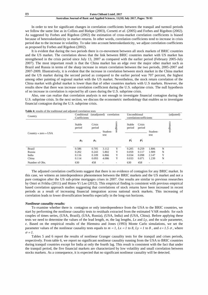
Tables 5 and 6 report the results of nonlinear Granger causality tests for the tranquil and crises periods,

respectively. From table 6, we report no significant nonlinear causality running from the USA to BRIC countries

during tranquil countries except for India at only the fourth lag. This result is consistent with the fact that under

the tranquil period, the five financial markets are characterized by low volatility and small correlation between

stocks markets. As a consequence, it is expected that no significant nonlinear causality will be detected.



Table 5: Nonlinear causality results from USA to BRIC countries (Tranquil period)

USA do not cause Brazil USA do not cause Russia USA do not cause India USA do not cause China

Lx=Ly CS TVAL CS TVAL CS TVAL CS TVAL

1 -0.669 -16.619 -0.468 -11.629 -0.618 -15.354 -0.610 -15.167

2 -0.465 -11.564 0.122 -3.029 -0.582 -14.449 -0.929 -23.096

3 -0.240 -5.981 -0.255 -6.349 -0.737 -18.315 -0.494 -12.284 4 -0.388 -9.645 -1.077 -26.757 0.092 -2.282 -0.053 -1.300

5 -0.272 -6.768 -0.245 -6.101 -0.029 -0.723 -0.225 -5.605

6 -0.045 -1.129 -0.136 -3.371 0.046 1.169 -0.288 -7.167 7 -0.473 -11.761 -0.286 -7.101 0.014 0.362 -0.308 -7.662

8 -0.566 -14.069 -0.646 -16.043 0.005 0.134 -0.356 -8.855

Note: CS and TVAL are, respectively, the difference between the two conditional probabilities and the Standardized test statistic. "Lx=Ly"

denotes the number of lags in the residual series used in the test. **,* indicate, respectively, significance at the 1% and 5%, levels.

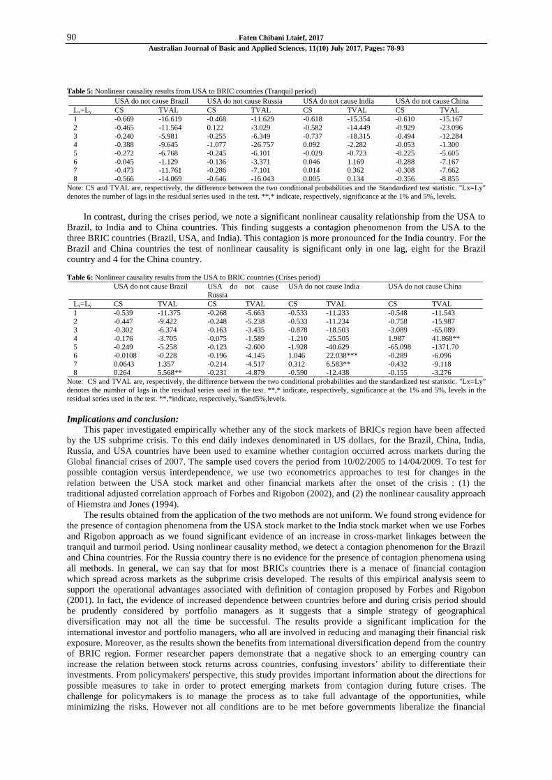
In contrast, during the crises period, we note a significant nonlinear causality relationship from the USA to

Brazil, to India and to China countries. This finding suggests a contagion phenomenon from the USA to the

three BRIC countries (Brazil, USA, and India). This contagion is more pronounced for the India country. For the

Brazil and China countries the test of nonlinear causality is significant only in one lag, eight for the Brazil

country and 4 for the China country.

Table 6: Nonlinear causality results from the USA to BRIC countries (Crises period)

USA do not cause Brazil USA do not cause Russia

USA do not cause India USA do not cause China

Lx=Ly CS TVAL CS TVAL CS TVAL CS TVAL

1 -0.539 -11.375 -0.268 -5.663 -0.533 -11.233 -0.548 -11.543

2 -0.447 -9.422 -0.248 -5.238 -0.533 -11.234 -0.758 -15.987 3 -0.302 -6.374 -0.163 -3.435 -0.878 -18.503 -3.089 -65.089

4 -0.176 -3.705 -0.075 -1.589 -1.210 -25.505 1.987 41.868**

5 -0.249 -5.258 -0.123 -2.600 -1.928 -40.629 -65.098 -1371.70 6 -0.0108 -0.228 -0.196 -4.145 1.046 22.038*** -0.289 -6.096

7 0.0643 1.357 -0.214 -4.517 0.312 6.583** -0.432 -9.118

8 0.264 5.568** -0.231 -4.879 -0.590 -12.438 -0.155 -3.276

Note: CS and TVAL are, respectively, the difference between the two conditional probabilities and the standardized test statistic. "Lx=Ly"

denotes the number of lags in the residual series used in the test. **,* indicate, respectively, significance at the 1% and 5%, levels in the

residual series used in the test. **,*indicate, respectively, %and5%,levels.

Implications and conclusion:

This paper investigated empirically whether any of the stock markets of BRICs region have been affected

by the US subprime crisis. To this end daily indexes denominated in US dollars, for the Brazil, China, India,

Russia, and USA countries have been used to examine whether contagion occurred across markets during the

Global financial crises of 2007. The sample used covers the period from 10/02/2005 to 14/04/2009. To test for

possible contagion versus interdependence, we use two econometrics approaches to test for changes in the

relation between the USA stock market and other financial markets after the onset of the crisis : (1) the

traditional adjusted correlation approach of Forbes and Rigobon (2002), and (2) the nonlinear causality approach

of Hiemstra and Jones (1994).

The results obtained from the application of the two methods are not uniform. We found strong evidence for

the presence of contagion phenomena from the USA stock market to the India stock market when we use Forbes

and Rigobon approach as we found significant evidence of an increase in cross-market linkages between the

tranquil and turmoil period. Using nonlinear causality method, we detect a contagion phenomenon for the Brazil

and China countries. For the Russia country there is no evidence for the presence of contagion phenomena using

all methods. In general, we can say that for most BRICs countries there is a menace of financial contagion

which spread across markets as the subprime crisis developed. The results of this empirical analysis seem to

support the operational advantages associated with definition of contagion proposed by Forbes and Rigobon

(2001). In fact, the evidence of increased dependence between countries before and during crisis period should

be prudently considered by portfolio managers as it suggests that a simple strategy of geographical

diversification may not all the time be successful. The results provide a significant implication for the

international investor and portfolio managers, who all are involved in reducing and managing their financial risk

exposure. Moreover, as the results shown the benefits from international diversification depend from the country

of BRIC region. Former researcher papers demonstrate that a negative shock to an emerging country can

increase the relation between stock returns across countries, confusing investors’ ability to differentiate their

investments. From policymakers' perspective, this study provides important information about the directions for

possible measures to take in order to protect emerging markets from contagion during future crises. The

challenge for policymakers is to manage the process as to take full advantage of the opportunities, while

minimizing the risks. However not all conditions are to be met before governments liberalize the financial



sector, countries should guarantee that the financial system is prepared to manage with foreign capital flows and

external shocks. More complete policies for risk management are needed to build solid economies, in particular

in terms of directive and administration of the financial system. The increasing integration of countries gives

governments less policy instruments to manage the shock, so there is a crucial need for international financial

policy coordination.

REFERENCES

Aloui, R., M.S.B. Aïssa and D.K. Nguyen, 2011. Global financial crisis, extreme interdependences, and

contagion effects: The role of economic structure? Journal of Banking & Finance, 35(1): 130-141.

Angkinand, A., E.M. Chiu and T.D. Willett, 2009. Testing the unstable middle and two corners hypotheses

about exchange rate regimes. Open Economies Review, 20(1): 61-83.

Antonakakis, N., I. Chatziantoniou and G. Filis, 2013. Dynamic co-movements of stock market returns,

implied volatility and policy uncertainty. Economics Letters, 120(1): 87-92.

Baek, E.G. and W.A. Brock, 1992. A nonparametric test for independence of a multivariate time series.

Statistica Sinica, pp; 137-156.

Baig, T. and I. Goldfajn, 1999. Financial market contagion in the Asian crisis. IMF Staff Papers, 46(2):

167-195.

Bekaert, G. and C.R. Harvey, 1997. Emerging equity market volatility. Journal of Financial Economics,

43(1): 29-77.

Beltratti, A., C. Morana and others, International shocks and national house prices, 2008. ICER-

International Centre for Economic Research.

Bertero, E. and C. Mayer, 1990. Structure and performance: the Global interdependence of stock markets

around the crash of October 1987∗. European Economic Review, 34(6): 1155-1180.

Billio, M. and L. Pelizzon, 2003. Volatility and shocks spillover before and after EMU in European stock

markets. Journal of Multinational Financial Management, 13(4): 323-340.

Bonfiglioli, A. and C.A. Favero, 2005. Explaining co-movements between stock markets: The case of US

and Germany. Journal of International Money and Finance, 24(8): 1299-1316.

Boyer, B.H., T. Kumagai and K. Yuan, 2006. How do crises spread? Evidence from accessible and

inaccessible stock indices. The Journal of Finance, 61(2): 957-1003.

Caillault, C. and D. Guegan, 2005. Empirical estimation of tail dependence using copulas: application to

Asian markets. Quantitative Finance, 5(5): 489-501.

Canarella, G. and S.K. Pollard, 2007. A switching ARCH (SWARCH) model of stock market volatility:

some evidence from Latin America. International Review of Economics, 54(4): 445-462.

Calvo, S.G. and C.M. Reinhart, 1996. Capital flows to Latin America: is there evidence of contagion

effects?

Celık, S., 2012. The more contagion effect on emerging markets: The evidence of DCC-GARCH model.

Economic Modelling, 29(5): 1946-1959.

Celikkol, H., S. Akkoc and Y.D. Akarim, 2010. The Impact of bankruptcy of Lehman Brothers on the

volatility structure of ISE-100 price index.

Chiang, T.C., B.N. Jeon and H. Li, 2007. Dynamic correlation analysis of financial contagion: Evidence

from Asian markets. Journal of International Money and Finance, 26(7): 1206-1228.

Corsetti, G., M. Pericoli and M. Sbracia, 2005. “Some contagion, some interdependence”: More pitfalls in

tests of financial contagion. Journal of International Money and Finance, 24(8): 1177-1199.

Corsetti, G., L. Dedola and S. Leduc, 2005. DSGE models of high exchange-rate volatility and low pass-

through.

Vaz de Melo Mendes, B., 2005. Asymmetric extreme interdependence in emerging equity markets. Applied

Stochastic Models in Business and Industry, 21(6): 483-498.

Diamandis, P.F., 2008. Financial liberalization and changes in the dynamic behaviour of emerging market

volatility: Evidence from four Latin American equity markets. Research in International Business and Finance,

22(3): 362-377.

Diebold, F.X. and K. Yilmaz, 2009. Measuring financial asset return and volatility spillovers, with

application to global equity markets. The Economic Journal, 119(534): 158-171.

Edwards, S. and R. Susmel, 2001. Volatility dependence and contagion in emerging equity markets. Journal

of Development Economics, 66(2): 505-532.

Engle, R., 2002. Dynamic conditional correlation: A simple class of multivariate generalized autoregressive

conditional heteroskedasticity models. Journal of Business & Economic Statistics, 20(3): 339-350.

Fidrmuc, J. and I. Korhonen, 2010. The impact of the global financial crisis on business cycles in Asian

emerging economies. Journal of Asian Economics, 21(3): 293-303.



Forbes, K.J. and R. Rigobon, 2002. No contagion, only interdependence: measuring stock market

comovements. The Journal of Finance, 57(5): 2223-2261.

Gagnon, L. and G.A. Karolyi, 2006. Price and volatility transmission across borders. Financial Markets,

Institutions & Instruments, 15(3): 107-158.

Gelos, R.G. and R. Sahay, 2001. Financial market spillovers in transition economies. Economics of

Transition, 9(1): 53-86.

Gilmore, C.K., S.E. McCarthy and E.S. Spelke, 2007. Symbolic arithmetic knowledge without instruction.

Nature, 447(7144): 589-591.

González-Hermosillo, B., 2008. Investors risk appetite and global financial market conditions.

Gómez-Puig, M. and S. Sosvilla-Rivero, 2013. Granger-causality in peripheral EMU public debt markets: A

dynamic approach. Journal of Banking & Finance, 37(11): 4627-4649.

Hamao, Y., R.W. Masulis and V. Ng, 1990. Correlations in price changes and volatility across international

stock markets. Review of Financial Studies, 3(2): 281-307.

Hamilton, J.D. and R. Susmel, 1994. Autoregressive conditional heteroskedasticity and changes in regime.

Journal of Econometrics, 64(1): 307-333.

Hsieh, D.A., 1991. Chaos and nonlinear dynamics: application to financial markets. The Journal of Finance,

46(5): 1839-1877.

Hsieh, D.A., 1989. Testing for nonlinear dependence in daily foreign exchange rates. Journal of Business,

339-368.

Khalid, A.M. and M. Kawai, 2003. Was financial market contagion the source of economic crisis in Asia?:

Evidence using a multivariate VAR model. Journal of Asian Economics, 14(1): 131-156.

Khallouli, W. and R. Sandretto, 2012. Testing for“ contagion” of the subprime crisis on the Middle East and

North African stock markets: A Markov Switching EGARCH approach. Journal of Economic Integration, pp:

134-166.

Khan, S. and K.W.K. Park, 2009. Contagion in the stock markets: The Asian financial crisis revisited.

Journal of Asian Economics, 20(5): 561-569.

Khan, S., F. Islam and S. Ahmed, 2005. The Asian crisis: an economic analysis of the causes. The Journal

of Developing Areas, 39(1): 169-190.

Karolyi, G.A. and R.M. Stulz, 1996. Why do markets move together? An investigation of US-Japan stock

return comovements. The Journal of Finance, 51(3): 951-986.

Kenourgios, D., A. Samitas and N. Paltalidis, 2011. Financial crises and stock market contagion in a

multivariate time-varying asymmetric framework. Journal of International Financial Markets, Institutions and

Money, 21(1): 92-106.

King, M.A. and S. Wadhwani, 1990. Transmission of volatility between stock markets. Review of Financial

Studies, 3(1): 5-33.

Lee, S.B. and K.J. Kim, 1993. Does the October 1987 crash strengthen the co-movements among national

stock markets? Review of Financial Economics, 3(1): 89.

Longin, F. and B. Solnik, 1995. Is the correlation in international equity returns constant: 1960–1990?

Journal of International Money and Finance, 14(1): 3-26.

Longin, F. and B. Solnik, 2001. Extreme correlation of international equity markets. The Journal of

Finance, 56(2): 649-676.

Longstaff, F.A., 2010. The subprime credit crisis and contagion in financial markets. Journal of Financial

Economics, 97(3): 436-450.

Loretan, M. and W.B. English, 2000. Evaluating correlation breakdowns during periods of market

volatility.

Yılmaz, M., 2015. Auctioning a discrete public good under incomplete information. Theory and Decision,

78(3): 471-500.

Masih, A.M. and R. Masih, 1999. Are Asian stock market fluctuations due mainly to intra-regional

contagion effects? Evidence based on Asian emerging stock markets. Pacific-Basin Finance Journal, 7(3): 251-

282.

Naoui, K., N. Liouane and S. Brahim, 2010. A dynamic conditional correlation analysis of financial

contagion: The case of the subprime credit crisis. International Journal of Economics and Finance, 2(3): 85-96.

Papavassiliou, V.G., 2014. Cross-asset contagion in times of stress. Journal of Economics and Business, 76:

133–139.

Patton, A.J., 2006. Modelling asymmetric exchange rate dependence. International Economic Review,

47(2): 527-556.

Pesaran, M.H., D. Pettenuzzo and A. Timmermann, 2006. Forecasting time series subject to multiple

structural breaks. The Review of Economic Studies, 73(4): 1057-1084.

Omri, A. and M. Frikha, 2011. No Contagion, Only Interdependence During the US Sub-Primes Crisis.

Transition Studies Review, 18(2): 286-298.



Ramlall, I., 2010. Has the US subprime crisis accentuated volatility clustering and leverage effects in major

international stock markets? International Research Journal of Finance and Economics, 39(13): 157-185.

Reinhart, C. and G. Kaminsky, 2000. Crisis financieras en Asia y Latinoamerica: ahora y entonces.

Rigobon, R., 2003. On the measurement of the international propagation of shocks: is the transmission

stable? Journal of International Economics, 61(2): 261-283.

Samitas, A. and I. Tsakalos, 2013. How can a small country affect the European economy? The Greek

contagion phenomenon. Journal of International Financial Markets, Institutions and Money, 25: 18-32.

Yiu, M.S., W.-Y. Alex Ho and D.F. Choi, 2010. Dynamic correlation analysis of financial contagion in

Asian markets in global financial turmoil. Applied Financial Economics, 20(4): 345-354.

Documents

Financial contagion in the BRIC countries during the 2007 ... · example, Baig and Goldfajn (1999) by using the correlation analysis test the presence of contagion in the equity,