Financial Dependencies, Environmental Regulation and

HAL Id: halshs-02423350https://halshs.archives-ouvertes.fr/halshs-02423350

Submitted on 24 Dec 2019

HAL is a multi-disciplinary open accessarchive for the deposit and dissemination of sci-entific research documents, whether they are pub-lished or not. The documents may come fromteaching and research institutions in France orabroad, or from public or private research centers.

L’archive ouverte pluridisciplinaire HAL, estdestinée au dépôt et à la diffusion de documentsscientifiques de niveau recherche, publiés ou non,émanant des établissements d’enseignement et derecherche français ou étrangers, des laboratoirespublics ou privés.

Financial Dependencies, Environmental Regulation andPollution Intensity: Evidence From China

Mathilde Maurel, Thomas Pernet, Zhao Ruili

To cite this version:Mathilde Maurel, Thomas Pernet, Zhao Ruili. Financial Dependencies, Environmental Regulationand Pollution Intensity: Evidence From China. 2019. �halshs-02423350�

https://halshs.archives-ouvertes.fr/halshs-02423350

https://hal.archives-ouvertes.fr

Documents de Travail du Centre d’Economie de la Sorbonne

Financial Dependencies, Environmental Regulation, and

Pollution Intensity: Evidence From China

Mathilde MAUREL, Thomas PERNET, Zhao RUILI

2019.29

Maison des Sciences Économiques, 106-112 boulevard de L'Hôpital, 75647 Paris Cedex 13 https://centredeconomiesorbonne.univ-paris1.fr/

ISSN : 1955-611X

Financial Dependencies, Environmental Regulation, andPollution Intensity: Evidence From China∗

Mathilde Maurel† Thomas Pernet‡ Zhao Ruili§

Abstract

We study how a bank’s involvement in a firm’s financing may be in line with environ-mental policies pursued by the Chinese central government. Specifically, we evaluatethe effectiveness of credit reallocation away from polluting projects when the govern-ment imposes stringent environmental policies. We combine the industries’ financialdependencies with time, including cross-cities variation in policy intensity to identifythe causal effect on the sulfur dioxide (SO2) emission. We find that SO2 emissions arelower in industries with high reliance on credits and stricter environmental regulations.Furthermore, our results suggest that locations with strong environmental policies leadfirms to seek funding in less regulated areas, which confirms the pollution haven hy-pothesis.Keywords: Banks, Financial Dependency, Environmental regulation, China

JEL Codes: F36, G20, Q53, Q56

∗We would like to thank the organizers (Etienne Le Rossignol and Candice Yandam) and participants ofthe Development Economics Sorbonne Informal Research Seminar (DESIR), but also the organizers of theJDD (Journees Doctorales du Developpement) hosted at Universite Paris Est Marne La Vallee and Neha BUpadhayay and Sebastien Marchand for their precious comments†CNRS, France and Centre d’Economie de la Sorbonne, Universite Paris 1 Pantheon-Sorbonne, France‡Centre d’Economie de la Sorbonne, Universite Paris 1 Pantheon-Sorbonne, France, email:

[email protected]§International Business School, Shanghai University of International Business and Economics, China

Documents de travail du Centre d'Economie de la Sorbonne - 2019.29

mailto:[email protected]

mailto:[email protected]

1 Introduction

The Global South, and more particularly China, is becoming increasingly responsible for

global warming. Consequently, there is a growing awareness that a few important emerging

countries such as China and India need to make a swift transition towards a cleaner model of

economic growth, which is particularly challenging given the fast increase in a consumption-

oriented middle class1. However, this challenge can also bring many opportunities. According

to the International Energy Agency’s World Energy Investment 2019 report, ”global power

investment is shifting towards emerging and developing countries [with] remarkable invest-

ment in renewable . . . In most regions, low-carbon sources were the largest part of generation

spending . . . [and] in India, total renewable power investment topped fossil fuel-based power

for the third year in a row”2.

Concern about environmental issues is also growing dramatically in China, which stands

out because of its environmental disasters and poor air quality3. China has experienced

numerous disasters, which impact the health of the population and nourish political discon-

tent. In addition, China is a major global air polluter and has had a significant increase in

the emission of sulfur dioxide (SO2) since its entry into the WTO in 2001, which reached

a peak in 2006. Interestingly, this trend has since been declining (see figure 1). This re-

duction coincides with the introduction of stringent environmental measures by the central

government.

Previous studies point to the improvement of environmental metrics by reallocating pro-

duction away from polluting sectors (Shi and Xu (2018); Chen et al. (2018); Hering and

1 OECD report, Development Matters 2019.2 IEA. World Energy Investment 2019. Paris: IEA, 2019.3China became the largest COD emitter in the world in 2006, surpassing the United States. In 2018,

China still held the first place. China also hosts more than half of the most polluted cities in the worldaccording to the WHO. For instance, in 2013, Shijiazhuang had only 47 days with good air quality. In 2017,China had the most natural disasters in the world, surpassing the United States and India. In the sameyear, the province of Hunan suffered a direct economic loss of about 59 billion RMB due to natural disasters(National Bureau of Statistics of China; Ministry of Ecology and Environment (China)). More statistics canbe found here.

1


https://www.iea.org/wei2019/

https://oecd-development-matters.org/2019/06/20/the-global-souths-contribution-to-the-climate-crisis-and-its-potential-solutions/

https://drive.google.com/open?id=16ftB1MMwn9drPqVb1b5O51ODzhPQjiW-

https://drive.google.com/open?id=1nq-njkZ-TaQyzH30Ncq1R8hlpFE1InSG

Poncet (2014)). However, except for Andersen (2016, 2017) and Earnhart and Segerson

(2012), little research has paid attention to the relationship between the financial system

and environmental issues. This paper aims to make a contribution to this area of research

by investigating the effectiveness of credit reallocation away from polluting projects in the

context of environmental policy change, or how a bank’s involvement in a firm’s financ-

ing may be in line with environmental policies pursued by the Chinese central government.

Banks indeed have a central role to play in promoting sustainable development—they finance

cleaner projects and help firms to adopt cleaner technology.

There is a large literature of firms’ environmental performance, in both developed (e.g.

Gray and Deily (1996); Cole et al. (2005); Shadbegian and Gray (2005); Earnhart and

Segerson (2012)) and developing countries (e.g. Earnhart and Lizal (2006); Cole et al.

(2008)). In this paper we focus on China because it is an ideal candidate to study the link

between financial dependency and environmental performance. Although it is relatively in-

efficient (Boyreau-Debray (2003); Dollar and Wei (2007)), the Chinese financial market went

through rapid reform over a short time span to cope with the transition to a market-driven

economy (Jarreau and Poncet (2014)). Banking assets form the majority of loans (i.e., about

85%), and are dominated by the four state-owned commercial banks (Allen et al. (2009)).

The entry of China to the WTO in 2001 triggered a rapid economic growth and environmental

degradation, which was caused by mismanagement of resources and mass industrialization.

However, China was not impacted equally, providing considerable spatial variations across

coastal and inner-land provinces, and giving our estimation strategy enough variability to

identify the link between financial performance and environmental regulations.

In this paper, we use the most extensive environmental statistics available in China. This

dataset is collected and maintained by the Ministry of Environmental Protection (MEP) and

it gathers information about the emission of major pollutants such as sulfur dioxide, which

is our variable of interest, wastewater, chemical oxygen demand, and industrial dust, and it

covers all industrial sectors. To our knowledge, only a few studies have used this thin level

2


of pollution emissions in China. We are able to track most of the industrial emissions of SO2

during six consecutive years (2002–2007) at the level of industries, provinces, and cities.

The 11th five-year plan (FYP) 4 was launched in 2006. It issued a set of quantitative

measures of pollution reduction targets at the national and local levels, which were spread

unequally across China, with some provinces being required to exert higher efforts while

others were required to make lower efforts. The sectoral financial dependency captures the

extent to which an industry needs to rely on external financing.

We conduct a difference-in-difference-in-difference (DDD) estimate to evaluate the effect

of the credit reallocation that was induced by the shift of policy emphasis towards environ-

mental concerns after 2006. Specifically, we compare the before and after variations of SO2

emissions by dividing the sample into pre- and post-treatment periods. We interact with

a time dummy that is equal to one after 2006 with the pollution reduction target and the

sectoral financial dependency. The advantage of the triple difference is the possibility to

include the full fixed effects of city-industry, city-year, and industry-year. The triple pairs of

fixed effects can alleviate the potential omitted variables from both the city and industry lev-

els across time. Thanks to market incentives and policy orientation, China’s banks are now

shifting the flow of capital into projects that are in line with the government’s environmental

objective of SO2 emission reduction.

Our results are twofold. First, we find strong evidence that financially more dependent

sectors with higher reduction targets emit less SO2, which confirms our hypothesis of a credit

shift in favor of sustainable finance. Our estimates show that an increase of the regulation

stringency by 1500 tons of SO2 above the cities means reduces the emission of SO2 by 3.54%.

It has also been shown by research for the European Commission 5 that the external damage

cost of one ton of SO2 is valued at $7228. Therefore, our computation shows that an average

city can save up to $29 million per year.

4The first FYP started in 1953, followed by nine plans until our study. More specifically, our analysisspans the years 2002 to 2007, both the 10th FYP (i.e., 2002-2005) and partially the 11th FYP (i.e., 2006-2007).

5Benefits Table database: Estimates of the marginal external costs of air pollution in Europe: link.

3


https://ec.europa.eu/environment/enveco/air/pdf/betaec02a.pdf

We also confirm that our results are not sensitive to outliers and are not driven by

the pre-trend effect. We also find that private versus state-owned enterprises (SOE), or

domestic versus foreign enterprises, do not react with the same intensity to the environmental

regulations.

Our results suggest that the government should act in favor of stringent and coordinated

environmental policies. As a result, market mechanisms will allocate efficiently capital for

sustainable finance.

Second, we test whether our results are in line with the growing literature on the pollution

haven hypothesis (PHH). Specifically, we construct a variable to capture the reallocation

effect. We then divide each city in our sample dataset based on whether the environmental

effort is large enough to provide an incentive for a firm to leave. Our results suggest that

a stronger deterrent effect of environmental regulation leads firms to seek funding in less

restricted provinces, confirming the pollution haven hypothesis (PVH). Our results are in

line with previous works in the area (Hering and Poncet (2014); Chen et al. (2018); Shi and

Xu (2018))

The rest of this paper is organized as follows. The institutional background of environ-

mental regulations in China is described in Section 2. Next, Section 3 discusses the data,

variables, and estimation strategy. Our empirical findings are presented in Section 4. Finally,

this paper concludes in Section 5.

2 Policy & environment

The reform of China began in 1953 with the implementation of the FYPs by the central gov-

ernment, including economic development and social balance. The FYP is a set of national

objectives that are initiated by the Communist Party of China and enforced by the local gov-

ernments. Severe environmental incidents in the mid-1960s pushed the central government

to address environmental issues more carefully. Although a decentralized system to control

4


SO2 emission in China from 2000 to 2010

Figure 1: Emission of SO2 in China for the period 2000 to 2010. Note: The horizontalline represents the beginning on the 11th FYP. Starting from 2006, China introducedmore environmental severity with an optimistic target of 10% reduction of SO2 emissionin 2010 compared with the level of 2005.Source: The SO2 emission data are from the China Statistical Yearbook (2000, 2010)

and prevent pollution has been operational since 1978, it has mainly been ineffective (Xu

et al. (2009)). Specific environmental regulations first appeared in the 9th FYP and they

were strengthened afterward 6. In the 10th FYP, a national objective of a 10% reduction of

the emissions of SO2 was established. To date, SO2 is one of the most significant sources of

air pollution in China (Yan and Wu (2017)). However, the bold objective of the 10th FYP

failed, mainly for three reasons. First, banks have always provided credit to large indus-

trial firms to promote industrialization, while paying little attention to the environmental

degradation caused by the growth process (The World Bank (2008)). Second, the State

Environmental Protection Administration (SEPA) was a weak regulatory agency (Stoerk

(2018)). And third, local governments were not under threat of sanctions if they failed. The

trade-off between growth and environmental warming is as binding in China as everywhere

in the world. Up to the 11th FYP, economic growth, employment, and tax revenue were the

key priorities of the local officials (Jiang et al. (2014); Chen et al. (2018)).

By the end of 2005, it was decided to enforce the 10% mandate in the framework of the

11th FYP and more constraints were put in place at the local level. Economic growth and

6The key features of environmental regulation are described in Xu (2011).

5


http://www.stats.gov.cn/english/Statisticaldata/AnnualData/

environmental objectives can be intertwined as long as the local government is responsible for

the outcomes. A round of negotiations took place between the central government and the

local government to allocate the pollution reduction mandates. Several different candidates

were introduced in the computation of the target. The final pollution reduction estimate

included economic growth, industrial structure, current pollution intensity, and geographic

location (i.e., East, Central, West). In May 2006, the local government and the SEPA agency

signed a contract to bind the reduction target (”The 11th Five-Year Plan: Targets, Paths

and Policy Orientation”)7. Following that statement, many provincial leaders decided to

distribute the burden across cities (Liu and Wang (2017))8. In July 2006, for instance, the

provincial government of Shanxi disaggregated the SO2 reduction mandate down to the 11

cities.

One of the key elements of the regulation is that local leaders’ career opportunities are

made dependent on the achievement of environmental objectives. A failure to meet the

pollution reduction mandate leads to the dismissal of the official or a downgrade from his or

her current position.

The Chinese government has shown its strong commitment to facilitate the tasks of the

local authorities. In addition to the existing environmental laws and regulations, market-

based policy instruments in favor of pollution reduction and environmental protection were

introduced. Not only did the Chinese government pour enormous public investment into this

problem but it also uses the financial markets to improve the environment. An improvement

of the communication between SEPA and commercial banks allowed them to limit or even

reject loans to firms infringing environmental laws (OECD (2008)). Furthermore, credit

administration institutions and SEPA developed strong ties that can restrain the access

of high energy consumption input industries, and also promote environmentally friendly

projects and emissions reduction. By the end of 2009, the total amount of investment geared

7The official statement is available here.8The government issued a document in 2006 with a clear guideline about the reduction allocation within-

province. The formula is explicit: ∆CODc,05−10 = ∆CODp,05−10 × Pc,2005∑Jj=1 Pj,2005

.

6


http://en.ndrc.gov.cn/newsrelease/200603/t20060323_63813.html

toward the environment reached 1.33% of China’s GDP, which represents a yearly increase

of 15% since 2005.

3 Empirical Strategy

The main objective of our empirical strategy is to assess the effect of credit reallocation on

the emission of pollution when banks face stringent environmental policies. We argue that

banks allocate resources to firms that comply with environmental regulations and with the

objectives of reducing pollution.

As mentioned in the section 2, Policy and environment, in 2006 lawmakers assigned

different levels of SO2 to cities, which should be met within the time span of the FYP.

The spatial heterogeneity of this policy and the existence of a treatment year (before and

after 2006) can be exploited to implement a difference-in-difference study and to identify the

effect of stricter environmental policies. Our identification strategy also relies on financial

dependency variability. We argue that firms who are dependent on banks are more likely to

react to the new regulation when banks confronted with the new regulation can reallocate

the credit away from polluting projects9.

This is reflected in the following equation, where we account for three levels of variability:

SO2ckt = αFinancial Dependenciesk×Postt×Reduction Mandatec+βXckt+µct+γkt+δck+εckt

(1)

Where SO2ckt is the level of SO2 in city c, for industry k and time t. The right-hand side

of the equation contains three main variables, a set of control variables and fixed effects.

Financial Dependenciesk reflects the financial dependency of industry k vis-a-vis banks.

9This DDD strategy has been used in different papers to tackle the endogeneity problem. For moredetails about the related papers, please refer to Hering and Poncet (2014); Cai et al. (2016); Chen et al.(2018); Shi and Xu (2018).

7


Postt is a dummy variable that takes the value of 1 when t is above 2005, and other-

wise is 0. This captures the two periods when the FYP takes place. Reduction Mandatec

is the measure of stringent environmental policies in city c. We add three control vari-

ables usually found in the literature (Andersen (2016, 2017)), which are the total outputckt,

total fixed assetckt, and employmentckt aggregated at the city c, industry k and time t. We

use the log of the emission of SO2 and aggregate the different variables at the two-digit in-

dustrial level because this is the lowest level where Financial Dependenciesk is available. The

equation includes city-year fixed effect µct. It controls for all city characteristics that differ

between cities through time, such as productivity, policies, wages. γkt is an industry-time

pair fixed effect that captures the intrinsic features of each industry within time like the

technological contents, subsidies. With δck, we address the industry’s invariant differences

between cities. In our equation εckt represents the error term.

Our strategy allows us to isolate the effect of stricter environmental policies before and

after the 11th FYP with the inclusion of the fixed effects. Our identification compares the

effect of stringent environmental regulation at different levels of financial dependencies on

the emissions of SO2. The coefficient α is associated with the triple interaction term and

it allows us to identify the effect of the treatment, namely the introduction of the 11th

FYP, after 2006. We expect this term to be negative and significant. Cities with stricter

targets should emit less SO2 during the second period of the analysis because the banks

have more incentive to finance firms that respect environmental policies. In all regressions,

the standard errors are two-way clustered by city and by industry. This enables spatial and

serial correlation of the error term.

8


4 Data and variables construction

4.1 SO2 data sources

The Ministry of Environmental Protection (MEP) has collected the main data source of

pollutants and wastes in China since 1980 10. The MEP has monitored firms in 39 major

industrial sectors that are considered as heavy polluters. These firms are asked to report

basic information, such as company name, address, and output. They also answer a very

detailed questionnaire about their emissions of major pollutants (e.g., wastewater, COD,

SO2, industrial smoke, and dust). As reported in Wu et al. (2017) and Jiang et al. (2014),

this dataset contains about 85% of the emissions of pollution from major pollutants in China.

The MEP has implemented strict procedures, including unforeseen visits from experts, to

ensure that these firms have not misreported their emissions. In our analysis, we have access

to the SO2 statistics, a primary air pollutant, for 289 two digits industries, spread across

284 cities from 2002 to 2007.

The primary air pollutants reached a peak of emission in 2005 at 32.41 million tons of SO2

(figure 1). Among the 522 cities monitored by the Chinese Ministry of Environment, about

400 had annual average SO2 levels that meet the Grade II national standard (0.06mg/m3)

11 and 33 cities met the worst grade (0.10mg/m3). Two years after the 11th FYP was

10The name of the database is “Chinese Environmental Statistical Database (CESD”. The database isprovided by the Ministery of Environmental Protection and kept very confidential.

11China uses its own air quality standard, which is less stringent than the WHO’s standard. China’sNational Environmental Monitoring Center (CNEMC) has a real-time, hourly air quality data for majorcities in China. The real-time data is available at here. Major air pollutants including SO2, NO2, and PM10are monitored. To evaluate air quality, the Chinese government applies three classes. Class 1 means theyearly SO2 level is less than 0.02 mg/m3, or a daily average of less than 0.05mg/m3. Class 2 is less restrictive.The yearly average should not exceed 0.06 and a daily average of about 0.15. Class 3 is complacent withbad air quality. The yearly average can exceed 0.10 mg/m3, and the daily average is 0.25. By contrast, theWHO recommends a daily average of less than 0.02mg/m3. For the records, exposure to high SO2 levelsdangerously affects health. According to the WHO ”SO2 can affect the respiratory system and the functionsof the lungs and causes irritation of the eyes. Inflammation of the respiratory tract causes coughing, mucussecretion, aggravation of asthma, and chronic bronchitis and makes people more prone to infections of therespiratory tract.”.

9


http://www.cnemc.cn/

https://www.who.int/news-room/fact-sheets/detail/ambient-(outdoor)-air-quality-and-health

launched, the situation had slightly changed according to the Ministry of Environment in

its annual report on the state of the environment in China 12. A total of 79% percent of

the audited cities met Grade II, which is two percentage points higher than in 2005. A

towering achievement concerned the Grade III criteria, where less than 1.2% of the cities

were above the threshold and represents four percentage points less than 2005. The most

polluted cities are located in Shanxi, Guizhou, Inner Mongolia, and Yunnan provinces. In

table 6 in the appendix, we computed the sum and average of the SO2 emission during both

periods. Overall, we note that the average SO2 level is lower during the treatment period

(10,714 - 10,432 tons).

4.2 City reduction mandate

The 11th FYP provides a general SO2 pollution reduction guideline for the provinces in

China. The provincial leaders have a binding contract with the Ministry of Environment

in which they bear the responsibility of any failure. To dilute the provincial objectives at

a lower administrative level, the local government decided to include the cities. In a recent

paper, (Chen et al. (2018)) use an official document to estimate pollution reduction mandate

at the city level. We replicate their methodology, which is based upon the following formula:

∆SO2c,05−10 = ∆SO2p,05−10 ×29∑k=1

µkoutput value of industry k in city c

output value of industry k in province p(2)

where, c stands for city, p for province and k for the two digits industry. The left-hand

side of the formula evaluates how much a city should reduce its SO2 emissions 2010 as

compared with 2005. For example, Shanghai intended to reduce its SO2 emissions by 13,000

tons in 2010.

12The report is available here.

10


http://english.mee.gov.cn/Resources/Reports/soe/soe2007/201

This estimate is computed by interacting with two components. The first component

is the official province reduction mandate and is expressed in ten thousand tons 13. This

measure is available for the 31 provinces of China. The second part is the share of industrial

production k, in city c over the total output of k in province p. A weight, µk, as the industry’s

proportion of total industrial SO2 emissions, is applied to account for the difference in SO2

intensity of each industrial sector.

We use the ASIF survey data to construct output share by industry for all the 298 cities

of our dataset. The SO2 industry share µk is measured from the MEP dataset using the

year 2005. Table 7 in the appendix reports the values of the 29 industrial share of µ. For

instance, the weight of Processing of Non-metallic Mineral Products is 0.23, which is the

largest in the sample, while in contrast textile has a coefficient of 0.04. The average of the

series is 0.034.

Table 1: SO2 emissions and control variables

Panel A: City-industry characteristics

All cities Coastal Southwest Central Northwest Northeast

SO2 10.619 8.071 18.349 10.797 14.493 5.729(1.000 tons) (38.967) (21.644) (62.603) (30.878) (69.606) (18.347)Output 9.31 13.237 7.882 6.868 6.412 6.947(10 millions USD) (15.264) (18.175) (13.788) (12.115) (12.201) (13.293)Fixed Asset 70.319 107.79 44.952 46.532 44.799 60.935(10 millions USD) (129.37) (170.661) (84.336) (80.473) (75.504) (125.573)Employment 87.566 151.077 47.399 55.559 41.581 51.515(10 millions) (175.665) (261.522) (70.894) (75.958) (61.494) (80.275)

Panel B: City characteristics


City Mandate 1.245 1.657 1.658 0.938 0.728 0.628(1.000 tons) (1.610) (1.731) (2.474) (1.078) (0.808) (0.739)

Total Cities 284 87 45 80 38 34Observations 25404 9314 3569 6971 2514 3036

Panel A provides a summary statistics for the variables that vary by city-industry-year. Panel B shows the key statisticfor the variable varying with city only. The first row represents the average by variables. The standard deviations arepresented in parentheses.Sources: MEP dataset and ASIF dataset. Author’s own computation

13Province p has the obligation to reduce the emission of pollution in 2010 by x thousands of tons comparedwith the level in 2005.

11


Table 1 gives a brief overview of the SO2 reduction target in the major area of China.

Following Wu et al. (2017), we split cities between Coastal, Southwest, Central, Northwest,

and Northwest 14. The Coastal area of China is composed of 10 provinces and has a total

of 87 cities. This area is the wealthiest part of China, and is where most of the national

production and foreign investment take place. The Southwestern area has five provinces and

45 cities, while the Central area has six provinces and 80 cities. The Northern part of China

is split into the Western area with six provinces and 38 cities and the Eastern area with

three provinces and 34 cities. The Coastal and Southwestern parts of China have to reduce

pollution by 16,600 tons, on average, before the end of the 11th FYP. The Central part of

China is confronted with an objective of 9,400 tons, closely followed by the Northwest and

Northeast.

4.3 A measure of sector-level reliance on external finance

To meet the production level, firms need to finance a fraction of the costs (fixed and variable).

We use the industry’s external finance dependency, which is defined as the exposure of

industry to the banks. The computation of the industry’s external finance dependency is

straightforward—it is the share of capital expenditure not financed with cash flow from

operations. Previous works have used US data to proxy for the exposure to external finance

(Rajan and Zingales (1998); Claessens and Laeven (2003); Kroszner et al. (2007)) and in the

context of China (Jarreau and Poncet (2014); Manova et al. (2015); Fan et al. (2015)). We

use the Chinese data and replicate the methodology proposed by Fan et al. (2015), who use

the ASIF dataset during the years 2004–2006 to aggregate the capital expenditure and cash

14The province breakdown follows the paper of Wu et al. (2017). The Central provinces are AnhuiHenan, Hubei, Hunan, Jiangxi, and Shanxi. The Coastal provinces are Beijing, Fujian, Guangdong, HainanHebei, Jiangsu, Shandong, Shanghai, Tianjin, and Zhejiang. The Northeastern provinces are Heilongjiang,Jilin, Liaoning. Northwest are Gansu, Inner Mongolia, Ningxia, Qinghai, Shaanxi, and Xinjiang. TheSouthwestern parts are Chongqing, Guangxi, Guizhou, Sichuan, Yunnan, and Xizang.

12


flow at the two digits industrial level. Fan et al. (2015) argue 15 that the financial pattern

between the US and China is almost similar. Tobacco is the least vulnerable sector in the US,

while it ranks second in China. The leather products industry is the second least vulnerable

in the US and the fifth least vulnerable in China. Table 7 in the appendix gives the value of

financial dependence for the 29 industries in China. The average value is -.57, and industries

with a high technological requirement are also the most vulnerable. The Petroleum industry

and Processing of Nuclear Fuel industries are at the bottom of the table, stressing their high

reliance on credit.

4.4 City industry variables: control

Recent papers have demonstrated the role of the factors of production on the deterioration of

the environment (Cole and Elliott (2003); Cole et al. (2008)). Furthermore, capital intensity

positively affects the emission and intensity of pollution (Hering and Poncet (2014); Ander-

sen (2017)). In addition, large industries generate more emissions of SO2. The National

Bureau of Statistics of China (NBS) collects manufacturing data for all non-state-owned-

enterprise with sales above RMB 5 million and state-owned-enterprise (SOE). The survey

contains detailed information about the name, address, four-digit CIC industry classifica-

tion, ownership, and financial variables, including output, sales, fixed assets. This dataset

is reliable for at least two reasons. First, since 1995 the NBS has used the firms’ survey

data to compute metrics such as GDP. Second, firms do not have incentives to misreport the

numbers. According to Chen et al. (2018), the NBS is not allowed to share information with

other agencies (e.g., tax agency, government, etc.). The NBS uses its industrial classification

to sort firms by sectors. Given that our data started in 2002 and ended in 2007, we can

use the 2002 GBT classification for each year of our sample data. The financial dependency

15Unlike the US methodology, which uses the median over time, the authors use the aggregate value fromthe Chinese data because about 68% of the observations have 0 capital expenditure.

13


variable is computed at the two-digit industrial level. To stay consistent with the financial

dependency variable, all of the industrial variables are computed at the two digits classi-

fication. We aggregate the total output by year and city for all the two-digit industries.

We also compute the total employment at the city-industry-year level. Finally, the ASIF

dataset gives the yearly total net fixed asset by firms. We use this information to compute

the city-industry-year total fixed asset. Table 1, panel A, shows the basic metrics about

total output, fixed asset, and employment for all the cities and also the spatial location.

4.5 A first glance at the structure of Chinese SO2 emitting indus-

tries

The level of SO2 emissions between sectors in China has remarkable variations. The objective

of this paper is to disentangle the different levels of pollution when a sector faces different

borrowing constraints. A bank’s incentive to finance a project is motivated not only by

the commercial aspect but also from the environmental pressure imposed with the local

government. More precisely, cities are imposed by different levels of environmental severity,

which is translated into maximum SO2 emissions allowed by the end of the 11th FYP, as

shown in Figure 2.

We plot the relationship between the city’s reduction target and the variation of SO2

emissions for 2005 and 2007 16. The x-axis represents the reduction target formulated by the

local government and implemented by the cities. Section 4.2, provides more details about the

formula that we used to estimate the city reduction mandate. For the y-axis, we computed

the log difference of SO2 emissions in 2005 and 2007. Values above 0 indicate a reduction

of SO2 emissions in 2007 compared with 2005. For the following graphs, we use the same

y-axis variable. The positive line shows that cities with stringent environmental regulations

put more effort into fighting pollution. Most of the cities decreased their emissions in 2007

16Variation is computed as follows: Log(SO2 emission in 2005 - SO2 emission in 2007)/(SO2 emission in 2005)).

14


Actual against targeted pollution reduction

Figure 2: SO2 Reduction Targets and Actual Pollution Reduction, at the city level, areestimated according to the methodology proposed in section 4.2. Note: Points in thefigures represent cities. Y-axis is Log(SO2 emission in 2005 - SO2 emission in 2007)/(SO2emission in 2005)). The line represents the fitted values. A positive trend indicates thatcities with stringent reduction mandate managed to reduce the level of SO2 emitted in2007 compared with 2005.Source: MEP Dataset. Author’s own computation

when compared to 2005, with a faster reduction for cities under environmental pressure. In

figure 3, we plot the industry financial dependencies against the industry changes in pollution

emission between 2005 and 2007. Financial dependency is borrowed from the paper of Fan

et al. (2015), who computed the borrowing constraints for 29 sectors in China. Sectors

with large values need to find funding from financial players. If Financial Dependency is

high, then the industry is more financially vulnerable and has a larger reliance on external

funding. Industries exposed to bank funding managed to lower their emissions of SO2 at

a faster speed. This suggests that the banks have reoriented loans in favor of sustainable

finance.

Our empirical approach links the financial dependencies with the stringency of the local

environmental regulation to understand the industrial and local changes in the emissions of

15


Reliance of financial dependency and success of reduction pollution

Figure 3: Financial Dependencies by sector and Actual Pollution Reduction. Note:Points in the figures represent 29 CIC sectors. Y-axis is Log(SO2 emission in 2005 - SO2emission in 2007)/(SO2 emission in 2005)). The line represents the fitted values. Apositive trend indicates that sectors relying on banks’ funding were more successful inreducing the level of SO2 emitted in 2007 compared with 2005.Sources: MEP Dataset and Fan et al. (2015). Author’s own computation

pollution. Figure 4 analyses the variations of SO2 emission by financially constrained sectors

of two cities with different environmental mandates. The city of Tangshan belongs in the

top decile of environmental severity. The city of Xiamen is in the third decile. Both cities

share similar GDP characteristics 17.

In line with our expectations, the contribution to lower SO2 emission is stronger for finan-

cially dependent sectors in cities with stringent mandates. This implies that the banks have

more incentives to screen sustainable projects when there is local environmental pressure.

17Tangshan is a largely industrial prefecture-level city in the northeast of Hebei province. Tangshan’sGDP was about 10,744,000 RMB in 2005. Xiamen is a port city on China’s southeast coast, across the straitfrom Taiwan. It encompasses two main islands and a region on the mainland. The GDP of Xiamen wasaround 10,065,830 RMB in 2005.

16


Financial dependencies and two economically identical cities with differentenvironmental regulations

Figure 4: Financial Dependencies by sector and Actual Pollution Reduction for twosimilar cities facing different reduction mandates. Note: Points in the figures represent 29CIC sectors. Y-axis is Log(SO2 emission in 2005 - SO2 emission in 2007)/(SO2 emissionin 2005)). The line represents the fitted values. A positive trend indicates that sectorsrelying on banks’ funding managed to reduce the level of SO2 emitted in 2007 comparedwith 2005. Both cities are similar in terms of GDP, Tangshan has to comply with anhigher mandate. As a result, the slope of the line is steeper, suggesting that the impact ofthe financial vulnerability is stronger.Sources: MEP Dateset and Fan et al. (2015). Author’s own computation

5 Results of the effect of financial dependencies on the

emission of SO2

5.1 Main results

Our primary interest is to assess the impact of credit access on the emissions of SO2 in

the context of tighter environmental regulations. Table 2 reports the baseline regression

(equation 1). Columns 1 and 2 focus on the log of SO2 emissions at the city-industry-year

level. Columns 3 and 4 focus on the log of SO2 emission divided by the value-added at

the city-industry-year level, which is called SO2 intensity. All of the regressions include an

17


extensive range of fixed effects to control for time, city, and industry characteristics.

Table 2: The effect of environmental regulation and financial dependency on the emission ofSO2, baseline regression

Ln SO2 Ln SO2 intensity

(1) (2) (3) (4)Financial dep.k x Post x SO2 mandatec −0.354∗ −0.514∗∗ −0.415∗ −0.601∗∗∗

(0.208) (0.200) (0.213) (0.207)Ln outputckt 0.509∗∗∗ 0.486∗∗∗ 0.473∗∗∗ 0.456∗∗∗

(0.027) (0.029) (0.026) (0.031)Ln fixed assetckt 0.034 0.049∗ −0.221∗∗∗ −0.214∗∗∗

(0.030) (0.026) (0.040) (0.035)Ln employmentckt 0.082∗∗ 0.076∗∗ −0.548∗∗∗ −0.547∗∗∗

(0.035) (0.038) (0.047) (0.055)

City-year fixed effects Yes Yes Yes YesIndustry-year fixed effects Yes Yes Yes YesCity-industry fixed effects Yes Yes Yes YesObservations 25,404 18,509 25,404 18,509R2 0.889 0.866 0.869 0.860

SO2 intensity is computed as the total SO2 emission by city-industry-year divided by valueadded. SO2 city mandate measures the total amount of SO2 a city needs to reduce bythe end of the 11th FYP. Columns 2 and 4 exclude the top and bottom 4 most pollutedsectors in 2002. * Significance at the 10%, ** Significance at the 5%, *** Significance atthe 1%. Heteroskedasticity-robust standard errors in parentheses are two-way clustered bycity and by industry.

The first row of table 2 represents our coefficient of interest, the interaction between the

sector reliance on external financing, environmental regulation, and the period of the 11th

FYP. All of the coefficients are negative and significant. The coefficient of the triple inter-

action term is larger for SO2 intensity, which suggests that the environmental performance

has to be scaled down according to the production scale. In columns 2 and 4, we ensure

that extreme sectors do not drive our results. Therefore, we removed the top and bottom

polluted sectors in 2002 18. The coefficients of SO2 and SO2 intensity become larger and

18We excluded the following four least (most) polluted sectors: Furniture, Artwork and Other Manu-facturing, Printing, Reproduction of Recording Media, Electrical Machinery and Equipment, Smelting andPressing of Non-ferrous Metals, Raw Chemical Materials and Chemical Products, Smelting and Pressing ofFerrous Metals and Non-metallic Mineral Products.

18


they remain significant at 5% and 10%, respectively. Overall, these results suggest that in a

highly regulated area, banks tend to re-allocate credits to firms that obey the environmental

policies.

The coefficient in column 1 means that the requirement of a reduction by one standard

deviation above the mean (which represents 1500 tons of SO2) leads to a reduction of pol-

lution emission by 3.54%. The mean pollution being set equal to 11,000 tons in 2005, this

implies a reduction of S02 emissions by 4000 tons (11.000 times 0.0354). Researchers have

estimated that the external damage cost of one ton of sulfur dioxide to be equivalent to

$7228 19. An increase of the reduction mandate by 1 standard deviation can therefore be

valued at 29 million USD per year (7228 x 4000).

To illustrate the difference between a sector that is financially dependent on credit rel-

ative to a sector that is not, we compare the value of the 10th percentile of the variable

Financial Dependencies and the 90th percentile. The 10th percentile in the data corre-

sponds to the Leather and fur industry, and the 90th is Paper. We set the increase of SO2

reduction mandate to 1.500 tons (roughly one standard deviation), and α = −.354. Taking

everything being equal, the key point is that the differential impact between the 90th and

10th percentiles of financial dependence 20 is equal to -7.19% for an increase of 1.500 tons of

SO2 mandate, which is strongly negative and significant 21.

In addition to the triple interaction terms and the fixed effects, our specification controls

for variables that vary across time, city, and industry. We include the output, fixed asset,

and employment variables aggregated at the city, industry year level. Rapid economic de-

velopment has severely degraded the environment. The coefficient of the output is highly

19This number, which represents the cost of SO2 emitted per ton in different years, varies across studies.Greenpeace estimates the cost of SO2 per ton to be $4356 for non-European countries. According to theOECD and for a sample of 14 European countries, it is about $9557. For the European Union, which refersto a city of 100,000 population, it reaches $7770. Therefore, we take the average of these three values in2007 for the year 2007 and we use the euro/USD exchange rate of 1.11.

20The value of the 10th quantile for Financial Dependencies is −1.11 and for the 90th quantile is 0.07.21The quantile point estimate formula is the following: value × α × (Financial Dependencies90th −

Financial Dependencies10th). The point estimate is calculated by 1500/10000 ∗ −.354 ∗ (0.03 + 1.324)) ∗ 100. −.354 is the α coefficient from table 2, column 1.

19


significant and positively correlated with SO2 and SO2 intensity, which puts high pressure on

the environment. Employment and fixed assets are positively correlated with SO2 and nega-

tively correlated with SO2 intensity. Including these variables does not affect our coefficient

of interest.

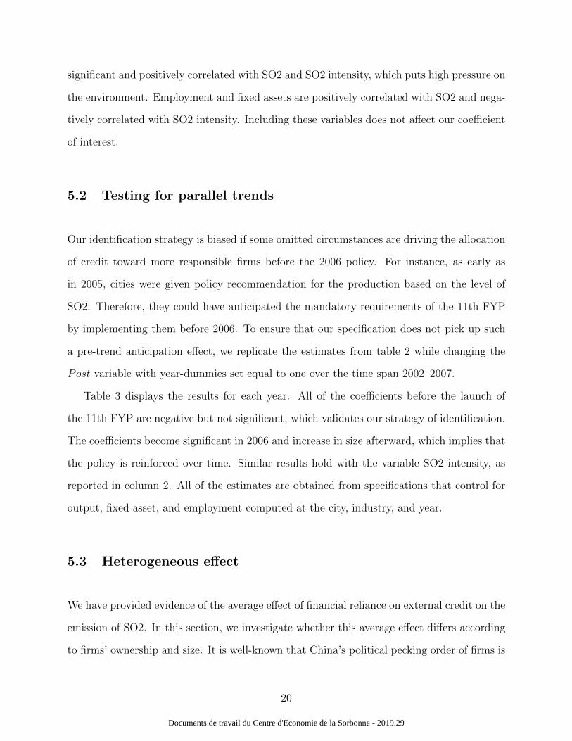
5.2 Testing for parallel trends

Our identification strategy is biased if some omitted circumstances are driving the allocation

of credit toward more responsible firms before the 2006 policy. For instance, as early as

in 2005, cities were given policy recommendation for the production based on the level of

SO2. Therefore, they could have anticipated the mandatory requirements of the 11th FYP

by implementing them before 2006. To ensure that our specification does not pick up such

a pre-trend anticipation effect, we replicate the estimates from table 2 while changing the

Post variable with year-dummies set equal to one over the time span 2002–2007.

Table 3 displays the results for each year. All of the coefficients before the launch of

the 11th FYP are negative but not significant, which validates our strategy of identification.

The coefficients become significant in 2006 and increase in size afterward, which implies that

the policy is reinforced over time. Similar results hold with the variable SO2 intensity, as

reported in column 2. All of the estimates are obtained from specifications that control for

output, fixed asset, and employment computed at the city, industry, and year.

5.3 Heterogeneous effect

We have provided evidence of the average effect of financial reliance on external credit on the

emission of SO2. In this section, we investigate whether this average effect differs according

to firms’ ownership and size. It is well-known that China’s political pecking order of firms is

20


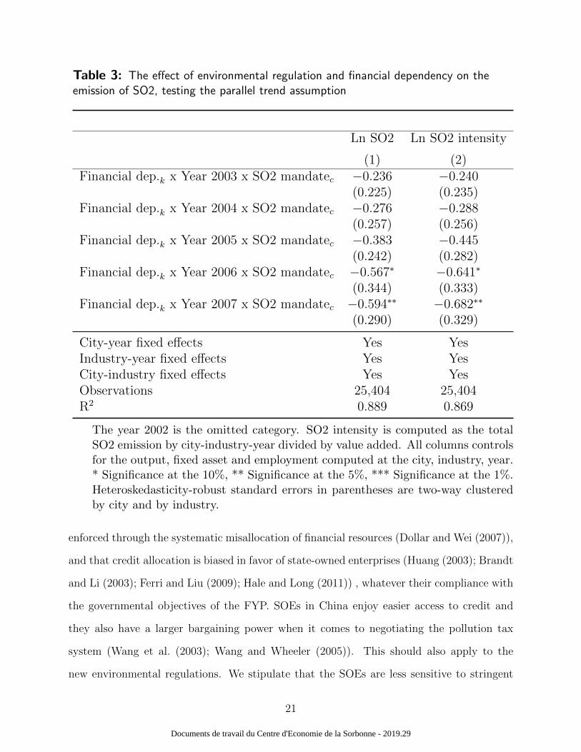
Table 3: The effect of environmental regulation and financial dependency on theemission of SO2, testing the parallel trend assumption


(1) (2)Financial dep.k x Year 2003 x SO2 mandatec −0.236 −0.240

(0.225) (0.235)Financial dep.k x Year 2004 x SO2 mandatec −0.276 −0.288

(0.257) (0.256)Financial dep.k x Year 2005 x SO2 mandatec −0.383 −0.445

(0.242) (0.282)Financial dep.k x Year 2006 x SO2 mandatec −0.567∗ −0.641∗

(0.344) (0.333)Financial dep.k x Year 2007 x SO2 mandatec −0.594∗∗ −0.682∗∗

(0.290) (0.329)

City-year fixed effects Yes YesIndustry-year fixed effects Yes YesCity-industry fixed effects Yes YesObservations 25,404 25,404R2 0.889 0.869

The year 2002 is the omitted category. SO2 intensity is computed as the totalSO2 emission by city-industry-year divided by value added. All columns controlsfor the output, fixed asset and employment computed at the city, industry, year.* Significance at the 10%, ** Significance at the 5%, *** Significance at the 1%.Heteroskedasticity-robust standard errors in parentheses are two-way clusteredby city and by industry.

enforced through the systematic misallocation of financial resources (Dollar and Wei (2007)),

and that credit allocation is biased in favor of state-owned enterprises (Huang (2003); Brandt

and Li (2003); Ferri and Liu (2009); Hale and Long (2011)) , whatever their compliance with

the governmental objectives of the FYP. SOEs in China enjoy easier access to credit and

they also have a larger bargaining power when it comes to negotiating the pollution tax

system (Wang et al. (2003); Wang and Wheeler (2005)). This should also apply to the

new environmental regulations. We stipulate that the SOEs are less sensitive to stringent

21


environmental regulations because of their stronger bargaining power and easier access to

bank funding, while private enterprises are forced to adjust by cutting and delocalizing their

production (Hering and Poncet (2014)).

We use the firms’ ownership information in the ASIF dataset to construct a list of a sector

dominated by SOEs. To do so, we aggregate the output by sector, year, and the type of firm

(i.e., private or state-owned). A sector is considered to be dominated by state ownership if

the share of SOEs in the total sectoral production is higher than the national median.

Column 1 in table 4 validates our assumption —SOEs are not affected by the environmen-

tal policies. This is reflected in the coefficient of the triple interaction term, which is negative

but not significant. However, we find that the regulation effect is large and significant for

industries dominated by private ownership.

There is a large body of the literature on external borrowing, particularly mentioning the

difference of credit access between domestic firms and foreign firms (Poncet et al. (2010);

Jarreau and Poncet (2014); Manova et al. (2015)). Foreign-owned companies are not confined

to borrow money in China because they can use funds from their parent company to raise

money on the capital market. Therefore, we seek to determine whether the regulation effect

may be different for sectors dominated by foreign and domestic firms. Columns 3 and 4

report the results for Log SO2 (Panel A) and SO2 intensity (Panel B). As expected, the

coefficient is negative but statistically insignificant for foreign industries, and it remained

negative and large for domestic industries.

In the last two columns, we estimate the effect of the size of the firm on access to

external borrowing (Beck and Demirguc-Kunt (2006)). A large number of empirical studies

show that large companies have easier access to external financing, which provides strong

evidence that financial market imperfection holds over a large range of countries and periods

of time, according to the Modigliani Miller theory of capital structure (Modigliani and Miller

(1958)). One primary reason for this is that large firms have more collateral to pledge

(Andersen (2016)). Similar evidence can be provided in our case and we thus expect large

22


Table 4: The effect of environmental regulation and financial dependency on the emission of SO2, Heterogeneouseffect

Panel A: Ln SO2

SOE Private Foreign Domestic Large Small

(1) (2) (3) (4) (5) (6)Financial dep.k x Post x SO2 mandatec −0.494 −0.413∗ −0.081 −0.716∗ −0.313∗∗ −0.513

(0.745) (0.227) (0.248) (0.366) (0.158) (0.749)

City-year fixed effects Yes Yes Yes Yes yes yesIndustry-year fixed effects Yes Yes Yes Yes yes yesCity-industry fixed effects Yes Yes Yes Yes yes yesObservations 6,216 19,188 7,614 17,790 21,014 4,390R2 0.957 0.903 0.941 0.897 0.895 0.921

Panel B: Ln SO2 intensity

SOE Private Foreign Domestic Large Small

(1) (2) (3) (4) (5) (6)Financial dep.k x Post x SO2 mandatec −0.531 −0.420∗ −0.163 −0.699∗ −0.357∗ −0.539

(0.765) (0.251) (0.311) (0.419) (0.184) (0.716)

City-year fixed effects Yes Yes Yes Yes yes yesIndustry-year fixed effects Yes Yes Yes Yes yes yesCity-industry fixed effects Yes Yes Yes Yes yes yesObservations 6,216 19,188 7,614 17,790 21,014 4,390R2 0.957 0.903 0.941 0.897 0.895 0.921

For columns 1-4, we aggregate the output by ownership (SOE/Private/Domestic/foreign), sector and year.For columns 5 and 6, we use the sales to estimate the size. We restrict the sample to industries whoseoutput/sales are higher than the yearly national median.SO2 intensity is computed as the total SO2 emission by city-industry-year divided by value added. Allcolumns controls for the output, fixed asset and employment computed at the city, industry, year level.* Significance at the 10%, ** Significance at the 5%, *** Significance at the 1%. Heteroskedasticity-robuststandard errors in parentheses are two-way clustered by city and by industry.

firms to be more sensitive to the environmental regulation channeled through banks. Large

versus small in the ASIF dataset is based upon the following proxy. We compute yearly sales

across industries considering industries to be dominated by large firms when its total annual

sales are above the sample median. Column 5 for Log SO2 (Panel A) and SO2 intensity

(Panel B) validates that the effect is statistically (in)-significant for large (small) industries.

23


5.4 Relocation effect

In this section, we provide additional evidence of the reduction of SO2 emissions channeled

through banks. We assume that environmental policies impose higher constraints on firms

in industries that rely on credit. We investigate whether or not firms seek to circumvent the

environmental regulation by relocating in cities with less environmental concerns and then

moving away part of their polluting activities from the more regulated cities. Banks in the

former cities do not discriminate against polluting firms (as they do in the later cities) by

redistributing the credit. Relocation activities in China are fast and straightforward thanks

to the recent industrial policies. According to Wang (2013) and Alder et al. (2016), the

government poured billions of RMB locally to develop infrastructure, build highways, and

improve the supply of utilities. In addition, the firm’s owners can decide to reduce the

production in cities with strict environmental policies and invest in factories located in areas

with lower environmental requirements.

The relocation effect is analyzed with a variable called relative reduction mandate which

seeks to measure the relative environmental effort required in city i as compared with all

other Chinese cities. It is simply the difference between city i’s reduction mandate minus

the reduction mandate averaged over all cities j22 except i, scaled by the output difference

between city i and cities j23. Then, we define a city with an incentive to downsize its

production in polluting industries targeted by banks if the relative reduction mandate is

above the mean 24. By interacting this variable with Financial dep and Post, we are able

to see whether banks induce banking-credit-dependent firms to move away from relatively

more regulated cities following the enforcement of the new regulation. If this hypothesis

22City i is not included in the list of cities j.23The formula to compute the index is (SO2 city mandatec/Outputc,2005) −

1/N∑J

j (SO2 city mandatej/Outputj,2005). The first part captures the city c effort, while the secondpart captures the average relative effort of cities j.

24Cities such as Shanghai, Beijing, Chongqing, Qingdao, Tianjin, Shenyang have all the incentive torelocate.

24


Table 5: The effect of environmental regulation and financial dependency on the emission ofSO2, reallocation effect


(1) (2)Financial dep.k x Post x SO2 mandatec −0.407∗∗ −0.469∗∗

(0.194) (0.200)Financial dep.k x Post x relative reduction mandatec −0.099∗∗ −0.098∗

(0.045) (0.051)

City-year fixed effects Yes YesIndustry-year fixed effects Yes YesCity-industry fixed effects Yes YesObservations 25,404 25,404R2 0.889 0.869

SO2 intensity is computed as the total SO2 emission by city-industry-year divided byvalue added. All columns controls for the output, fixed asset and employment computedat the city, industry, year.* Significance at the 10%, ** Significance at the 5%, *** Significance at the 1%.Heteroskedasticity-robust standard errors in parentheses are two-way clustered by cityand by industry.

holds, then the coefficient of the triple interaction term must be negative. Table 5 confirms

the double role played by financial intermediaries: the first interaction term confirms that

the allocation of funds goes toward environmentally friendly projects after 2006. The second

interaction term implies that the decrease in pollution results in a haven effect where more-

polluting firms are pushed away from more demanding cities in terms of S02 emissions. This

haven effect is supported by all measures of pollution (i.e., Log SO2 or SO2 intensity). Our

results echo the paper of Chen et al. (2018), who found a spatial transfer of water-polluting

activity.

25


6 Conclusion

This paper investigates the relationship between external borrowing and production-generated

pollution emission after a change in China’s environmental regulations.

The spatial and temporal variations of the environmental policy enacted by the 11th

FYP allow us to isolate the impact of financial dependency on the emission of air pollution.

We use a comprehensive dataset that includes the major pollutants in China, collected by

the Ministry of Environment. We find evidence that stricter environmental policies lead to

a deeper decline in emissions of SO2 in industries that are dependent on external borrowing.

Our results suggest that banks have more incentives to provide funding to firms that comply

with the environmental objectives announced by the government. Several robustness checks

confirm our findings. The effect of credit reallocation has more significant impacts on indus-

tries dominated by private, domestic, and large firms. Moreover, the spatial disparity of the

regulation leads firms operating in stringent areas to look for funding in cities where banks

are less preoccupied with the use of capital on the environment.

Pollution reduction is a notable concern in China. Every five years, the government

introduces stricter environmental regulations. Our paper shows that financial institutions

are vital players because they screen projects and choose to fund those projects that comply

with environmental policies. However, the mobility of firms can shift the burden to locations

where the regulations are more lax, leaving aside the banks’ responsibility regarding the

environment.

26


References

Alder, S., L. Shao, and F. Zilibotti (2016, December). Economic reforms and industrialpolicy in a panel of chinese cities. J. Econ. Growth 21 (4), 305–349.

Allen, F., M. Qian, M. Zhao, and Others (2009). A review of china’s financial system andinitiatives for the future. In China’s emerging financial markets, pp. 3–72. Springer.

Andersen, D. C. (2016, June). Credit constraints, technology upgrading, and the envi-ronment. Journal of the Association of Environmental and Resource Economists 3 (2),283–319.

Andersen, D. C. (2017, July). Do credit constraints favor dirty production? theory andplant-level evidence. J. Environ. Econ. Manage. 84, 189–208.

Beck, T. and A. Demirguc-Kunt (2006, November). Small and medium-size enterprises:Access to finance as a growth constraint. Journal of Banking & Finance 30 (11), 2931–2943.

Boyreau-Debray, G. (2003, April). Financial Intermediation and Growth: Chinese Style.Policy Research Working Papers. The World Bank.

Brandt, L. and H. Li (2003, September). Bank discrimination in transition economies:ideology, information, or incentives? J. Comp. Econ. 31 (3), 387–413.

Cai, X., Y. Lu, M. Wu, and L. Yu (2016, November). Does environmental regulation driveaway inbound foreign direct investment? evidence from a quasi-natural experiment inchina. J. Dev. Econ. 123, 73–85.

Chen, Z., M. E. Kahn, Y. Liu, and Z. Wang (2018, March). The consequences of spatiallydifferentiated water pollution regulation in china. J. Environ. Econ. Manage. 88, 468–485.

Claessens, S. and L. Laeven (2003, December). Financial development, property rights, andgrowth. The Journal of Finance 58 (6), 2401–2436.

Cole, M. and R. Elliott (2003). Determining the trade-environment composition effect: therole of capital, labor and environmental regulations. J. Environ. Econ. Manage. 46 (3),363–383.

Cole, M. A., R. J. R. Elliott, and K. Shimamoto (2005, July). Industrial characteristics,environmental regulations and air pollution: an analysis of the UK manufacturing sector.J. Environ. Econ. Manage. 50 (1), 121–143.

Cole, M. A., R. J. R. Elliott, and S. Wu (2008). Industrial activity and the environment inchina: An industry-level analysis. China Econ. Rev. 19 (3), 393–408.

Dollar, D. and S.-J. Wei (2007, May). Das (wasted) kapital: Firm ownership and investmentefficiency in china. Technical report, National Bureau of Economic Research, Cambridge,MA.

Earnhart, D. and L. Lizal (2006, March). Effects of ownership and financial performance oncorporate environmental performance. J. Comp. Econ. 34 (1), 111–129.

Earnhart, D. and K. Segerson (2012). The influence of financial status on the effectivenessof environmental enforcement. J. Public Econ. 96 (9-10), 670–684.

Fan, H., E. L.-C. Lai, and Y. A. Li (2015, May). Credit constraints, quality, and exportprices: Theory and evidence from china. J. Comp. Econ. 43 (2), 390–416.

Ferri, G. and L.-G. Liu (2009, April). Honor Thy Creditors Beforan Thy Shareholders: Arethe Profits of Chinese State-Owned Enterprises Real? Working Papers 162009, Hong

27


Kong Institute for Monetary Research.Gray, W. B. and M. E. Deily (1996, July). Compliance and enforcement: Air pollution

regulation in the U.S. steel industry. J. Environ. Econ. Manage. 31 (1), 96–111.Hale, G. and C. Long (2011). Chapter 13 what are the sources of financing for chinese firms?

In Emerald Group Publishing Limited (Ed.), The Evolving Role of Asia in Global Finance,Volume 9, pp. 313–339. emeraldinsight.com.

Hering, L. and S. Poncet (2014, September). Environmental policy and exports: Evidencefrom chinese cities. J. Environ. Econ. Manage. 68 (2), 296–318.

Huang, Y. (2003, January). One country, two systems: Foreign-invested enterprises anddomestic firms in china. China Econ. Rev. 14 (4), 404–416.

Jarreau, J. and S. Poncet (2014). Credit constraints, firm ownership and the structure ofexports in china. International Economics 139 (139), 152–173.

Jiang, L., C. Lin, and P. Lin (2014, February). The determinants of pollution levels: Firm-level evidence from chinese manufacturing. J. Comp. Econ. 42 (1), 118–142.

Kroszner, R. S., L. Laeven, and D. Klingebiel (2007, April). Banking crises, financial depen-dence, and growth. J. financ. econ. 84 (1), 187–228.

Liu, Q. and Q. Wang (2017, January). How china achieved its 11th Five-Year plan emissionsreduction target: A structural decomposition analysis of industrial SO2 and chemicaloxygen demand. Sci. Total Environ. 574, 1104–1116.

Manova, K., S.-J. Wei, and Z. Zhang (2015). Firm exports and multinational activity undercredit constraints. Rev. Econ. Stat. 97 (3), 574–588.

Modigliani, F. and M. H. Miller (1958). The cost of capital, corporation finance and thetheory of investment. Am. Econ. Rev. 48 (3), 261–297.

OECD (2008, December). Environmentally responsible corporate conduct in china. In OECD(Ed.), OECD Investment Policy Reviews: China 2008, pp. 257–284. OECD.

Poncet, S., W. Steingress, and H. Vandenbussche (2010, September). Financial constraintsin china: Firm-level evidence. China Econ. Rev. 21 (3), 411–422.

Rajan, R. and L. Zingales (1998). Financial dependence and growth. American EconomicReview 88 (3), 559–586.

Shadbegian, R. J. and W. B. Gray (2005). Pollution abatement expenditures and plant-levelproductivity: A production function approach. Ecol. Econ. 54 (2-3), 196–208.

Shi, X. and Z. Xu (2018, May). Environmental regulation and firm exports: Evidence fromthe eleventh Five-Year plan in china. J. Environ. Econ. Manage. 89, 187–200.

Stoerk, T. (2018). Effectiveness and cost of air pollution control in china. Technical report,London School of Economics.

The World Bank (2008, December). China - mid-term evaluation of china’s eleventh five-yearplan. Technical Report 46355, The World Bank.

Wang, H., N. Mamingi, B. Laplante, and S. Dasgupta (2003, March). Incomplete enforce-ment of pollution regulation: Bargaining power of chinese factories. Environ. Resour.Econ. 24 (3), 245–262.

Wang, H. and D. Wheeler (2005, January). Financial incentives and endogenous enforcementin china’s pollution levy system. J. Environ. Econ. Manage. 49 (1), 174–196.

Wang, J. (2013, March). The economic impact of special economic zones: Evidence fromchinese municipalities. J. Dev. Econ. 101, 133–147.

Wu, H., H. Guo, B. Zhang, and M. Bu (2017, February). Westward movement of new

28


polluting firms in china: Pollution reduction mandates and location choice. J. Comp.Econ. 45 (1), 119–138.

Xu, Y. (2011). The use of a goal for SO2 mitigation planning and management in china’s11th Five-Year plan. J. Environ. Planning Manage. 54 (6), 769–783.

Xu, Y., R. H. Williams, and R. H. Socolow (2009, May). China’s rapid deployment of SO2scrubbers. Energy Environ. Sci. 2 (5), 459–465.

Yan, S. and G. Wu (2017, April). SO2 emissions in china - their network and hierarchicalstructures. Sci. Rep. 7 (7), 46216.

Appendix

Table 6: Summary Statistics

Panel A: City-industry characteristics, Pre-treatment

All cities Coastal Southwest Central Northwest NortheastSO2 10.714 8.287 18.603 10.769 14.927 5.427(1.000 tons) 41.972 22.143 67.687 32.223 79.032 18.555Output 8.316 11.952 6.974 5.963 5.756 6.23(10 millions USD) 14.154 16.97 12.541 11.06 11.469 12.373Fixed Asset 65.328 99.288 43.921 42.275 43.305 57.32(10 millions USD) 121.193 156.946 85.527 75.01 76.266 123.671Employment 8.518 14.38 4.85 5.475 4.368 5.148(10 millions) 16.306 23.926 0.744 7.438 6.612 8.147

Panel B: City characteristics, Post-treatment


SO2 10.423 7.625 17.851 10.858 13.675 6.313(1.000 tons) 31.93 20.571 51.204 27.697 47.009 17.934Output 11.348 15.896 9.663 8.857 7.647 8.335(10 millions USD) 17.142 20.19 15.808 13.959 13.392 14.822Fixed Asset 80.562 125.389 46.976 55.895 47.612 67.936(10 millions USD) 144.177 194.876 81.947 90.662 74.009 128.948Employment 9.246 16.615 4.525 5.733 3.763 5.158(10 millions) 19.897 30.192 6.347 7.795 5.147 7.843

Panel A provides a summary statistics for the variables that vary by city-industry-year For the year 2002-2005 included. It is the pre-treatment period. Panel A provides a summary statistics for the variables that vary by city-industry-year For the year 2006-2007 . It isthe post-treatment period.The first row represents the average by variables. The Standard deviations are presented in parenthesesSources: MEP dataset and ASIF dataset. Author’s own computation

29


Table 7: SO2 Industry share, 2005

CIC Value

Non-metallic Mineral Products 31 0.2340Smelting and Pressing of Ferrous Metals 32 0.1983Raw Chemical Materials and Chemical Products 26 0.1611Processing of Petroleum, Coking, Processing of Nuclear Fuel 25 0.0910Smelting and Pressing of Non-ferrous Metals 33 0.0855Paper and Paper Products 22 0.0577Textile 17 0.0407Chemical Fibers 28 0.0222Processing of Food from Agricultural Products 13 0.0199Beverages 15 0.0130Foods 14 0.0123Medicines 27 0.0089General Purpose Machinery 35 0.0089Processing of Timber, Manufacture of Wood,Bamboo, Rattan, Palm, and Straw Products 20 0.0065Rubber 29 0.0063Transport Equipment 37 0.0061Special Purpose Machinery 36 0.0050Electrical Machinery and Equipment 39 0.0038Metal Products 34 0.0037Leather, Fur, Feather and Related Products 19 0.0029Communication Equipment, Computers and Other Electronic Equipment 40 0.0025Textile Wearing Apparel, Footwear, and Caps 18 0.0022Measuring Instruments and Machinery for Cultural Activity and Office Work 41 0.0020Plastics 30 0.0018Tobacco 16 0.0016Artwork and Other Manufacturing 42 0.0007Furniture 21 0.0006Articles For Culture, Education and Sport Activity 24 0.0004Printing, Reproduction of Recording Media 23 0.0004

The share is computed for 28 industries.Source: MEP dataset. Author’s own computation

30


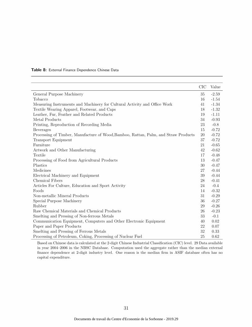
Table 8: External Finance Dependence Chinese Data

CIC Value

General Purpose Machinery 35 -2.59Tobacco 16 -1.54Measuring Instruments and Machinery for Cultural Activity and Office Work 41 -1.34Textile Wearing Apparel, Footwear, and Caps 18 -1.32Leather, Fur, Feather and Related Products 19 -1.11Metal Products 34 -0.93Printing, Reproduction of Recording Media 23 -0.8Beverages 15 -0.72Processing of Timber, Manufacture of Wood,Bamboo, Rattan, Palm, and Straw Products 20 -0.72Transport Equipment 37 -0.72Furniture 21 -0.65Artwork and Other Manufacturing 42 -0.62Textile 17 -0.48Processing of Food from Agricultural Products 13 -0.47Plastics 30 -0.47Medicines 27 -0.44Electrical Machinery and Equipment 39 -0.44Chemical Fibers 28 -0.41Articles For Culture, Education and Sport Activity 24 -0.4Foods 14 -0.32Non-metallic Mineral Products 31 -0.29Special Purpose Machinery 36 -0.27Rubber 29 -0.26Raw Chemical Materials and Chemical Products 26 -0.23Smelting and Pressing of Non-ferrous Metals 33 -0.1Communication Equipment, Computers and Other Electronic Equipment 40 0.02Paper and Paper Products 22 0.07Smelting and Pressing of Ferrous Metals 32 0.33Processing of Petroleum, Coking, Processing of Nuclear Fuel 25 0.62

Based on Chinese data is calculated at the 2-digit Chinese Industrial Classification (CIC) level. 29 Data availablein year 2004–2006 in the NBSC Database. Computation used the aggregate rather than the median externalfinance dependence at 2-digit industry level. One reason is the median firm in ASIF database often has nocapital expenditure.

31


List Figures/tables

List of Figures

1 Emission of SO2 in China for the period 2000 to 2010. Note: The horizontal line

represents the beginning on the 11th FYP. Starting from 2006, China introduced

more environmental severity with an optimistic target of 10% reduction of SO2

emission in 2010 compared with the level of 2005. Source: The SO2 emission data

are from the China Statistical Yearbook (2000, 2010) . . . . . . . . . . . . . . . 52 SO2 Reduction Targets and Actual Pollution Reduction, at the city level, are es-

timated according to the methodology proposed in section 4.2. Note: Points in

the figures represent cities. Y-axis is Log(SO2 emission in 2005 - SO2 emission in

2007)/(SO2 emission in 2005)). The line represents the fitted values. A positive

trend indicates that cities with stringent reduction mandate managed to reduce

the level of SO2 emitted in 2007 compared with 2005. Source: MEP Dataset.

Author’s own computation . . . . . . . . . . . . . . . . . . . . . . . . . . . . . 153 Financial Dependencies by sector and Actual Pollution Reduction. Note: Points

in the figures represent 29 CIC sectors. Y-axis is Log(SO2 emission in 2005 - SO2

emission in 2007)/(SO2 emission in 2005)). The line represents the fitted values. A

positive trend indicates that sectors relying on banks’ funding were more successful

in reducing the level of SO2 emitted in 2007 compared with 2005. Sources: MEP

Dataset and Fan et al. (2015). Author’s own computation . . . . . . . . . . . . . 164 Financial Dependencies by sector and Actual Pollution Reduction for two similar

cities facing different reduction mandates. Note: Points in the figures represent

29 CIC sectors. Y-axis is Log(SO2 emission in 2005 - SO2 emission in 2007)/(SO2

emission in 2005)). The line represents the fitted values. A positive trend indicates

that sectors relying on banks’ funding managed to reduce the level of SO2 emitted

in 2007 compared with 2005. Both cities are similar in terms of GDP, Tangshan

has to comply with an higher mandate. As a result, the slope of the line is steeper,

suggesting that the impact of the financial vulnerability is stronger. Sources: MEP

Dateset and Fan et al. (2015). Author’s own computation . . . . . . . . . . . . 17

List of Tables

1 SO2 emissions and control variables . . . . . . . . . . . . . . . . . . . . . . . . 112 The effect of environmental regulation and financial dependency on the emission of

SO2, baseline regression . . . . . . . . . . . . . . . . . . . . . . . . . . . . . . 183 The effect of environmental regulation and financial dependency on the emission of

SO2, testing the parallel trend assumption . . . . . . . . . . . . . . . . . . . . . 214 The effect of environmental regulation and financial dependency on the emission of

SO2, Heterogeneous effect . . . . . . . . . . . . . . . . . . . . . . . . . . . . . 23

32


http://www.stats.gov.cn/english/Statisticaldata/AnnualData/

5 The effect of environmental regulation and financial dependency on the emission of

SO2, reallocation effect . . . . . . . . . . . . . . . . . . . . . . . . . . . . . . . 256 Summary Statistics . . . . . . . . . . . . . . . . . . . . . . . . . . . . . . . . . 297 SO2 Industry share, 2005 . . . . . . . . . . . . . . . . . . . . . . . . . . . . . . 308 External Finance Dependence Chinese Data . . . . . . . . . . . . . . . . . . . . 31

33
