Financial development and dynamic investment behavior ...siteresources.worldbank.org/DEC/Resources/...investment_Behaviour.pdf · Financial development and dynamic investment behavior:

The Quarterly Review of Economics and Finance46 (2006) 190–210

Financial development and dynamic investmentbehavior: Evidence from panel VAR

Inessa Love a, Lea Zicchino b,∗a World Bank, Research Department—Finance Group, 1818 Hst, NW, MC3-300,

Washington, DC 20433, United Statesb Bank of England, Monetary Instruments and Markets Division, HO-2,

Threadneedle Street, London EC2R 8AH, UK

Received 14 April 2004; received in revised form 31 October 2005; accepted 4 November 2005

Abstract

We apply vector autoregression (VAR) to firm-level panel data from 36 countries to study the dynamicrelationship between firms’ financial conditions and investment. By using orthogonalized impulse-responsefunctions we are able to separate the ‘fundamental factors’ (such as marginal profitability of investment)from the ‘financial factors’ (such as availability of internal finance) that influence the level of investment. Wefind that the impact of financial factors on investment, which indicates the severity of financing constraints,is significantly larger in countries with less developed financial systems. Our finding emphasizes the role offinancial development in improving capital allocation and growth.© 2006 Board of Trustees of the University of Illinois. All rights reserved.

Keywords: Financial development; Vector autoregression; Dynamic investment behavior

1. Introduction

Unlike the neoclassical theory of investment, the literature based on asymmetric informationemphasizes the role played by moral hazard and adverse selection problems in a firm’s decisionto invest in physical and human capital. The presence of asymmetric information means that theclassical dichotomy between real and financial variables may no longer hold. Financial variablescan have an impact on real variables, such as the level of investment and the real interest rate, as wellas propagate and amplify the effects of exogenous shocks to the economy. For example, Bernanke

∗ Corresponding author. Tel.: +44 20 7601 5212; fax: +44 20 7601 3217.E-mail address: [email protected] (L. Zicchino).

1062-9769/$ – see front matter © 2006 Board of Trustees of the University of Illinois. All rights reserved.doi:10.1016/j.qref.2005.11.007

mailto:[email protected]

dx.doi.org/10.1016/j.qref.2005.11.007

I. Love, L. Zicchino / The Quarterly Review of Economics and Finance 46 (2006) 190–210 191

and Gertler (1989) show that a firm’s net worth (a financial variable) can be used as collateral inorder to reduce the agency cost associated with the presence of asymmetric information betweenlenders and borrowers. In this model, firms’ investment decisions are not only dependent on thepresent value of future marginal productivity of capital, as the q-theory predicts, but also on thelevel of collateral available to the firms when they enter a loan contract.

Since economists started to look at real phenomena abstracting from the Arrow-Debreuframework with its frictionless capital markets, a vast literature has been developed on the rela-tionship between investment decisions and firms’ financing constraints (see Hubbard, 1998, fora review). Even though asymmetric information between borrowers and lenders may be notthe only source of imperfection in the credit markets, firms seem to prefer internal to externalfinance to fund their investments. This observation leads to the prediction of a positive relation-ship between investment and internal finance. The first study on panel data by Fazzari, Hubbard,and Peterson (1988) finds that, after controlling for investment opportunities with Tobin’s q,changes in net worth have a greater impact on investment by firms with higher costs of externalfinancing.

The link between the cost of external financing and investment decisions not only sheds lighton the dynamics of business cycles but also represents an important element in understandingeconomic development and growth. For instance, in the presence of moral hazard in the creditmarket, firms that need a bank loan may be induced to undertake risky investment projects withlow expected marginal productivity. This corporate decision affects the growth path of the econ-omy, which may even fall into a poverty trap (see Zicchino, 2001). Rajan and Zingales (1998),Demirguc-Kunt and Maksimovic (1998) and Wurgler (2000), among others, have investigated thelink between finance and growth by asking whether underdeveloped legal and financial systemscould prevent firms from investing in potentially profitable growth opportunities. Their empiricalresults show that an active stock market, developed financial intermediaries and the respect oflegal norms are determinants of economic growth.

Estimation of the relationship between investment and financial variables is challengingbecause it is difficult for an econometrician to observe firms’ net worth and investment oppor-tunities. In theory, the measure of investment opportunities is the present value of expectedfuture profits from additional capital investment, or what is commonly called marginal q. Thisis the shadow value of an additional unit of capital and, under certain conditions, it can beshown to be a sufficient statistic for investment (Hayashi, 1982). In other words, it is the‘fundamental’ factor that determines investment policy of profit-maximizing firms in efficientmarkets. The difficulty in measuring marginal q, which is not observable, results in low explana-tory power of the q-models and, typically, entails implausible estimates of the adjustment costparameters.1

Another challenge is finding an appropriate measure for the ‘financial’ factors that enter theinvestment equation in models with capital markets imperfections. A widely used measure forthe availability of internal funds is cash flow (current revenues less expenses and taxes, gen-erally scaled by capital). However, cash flow is likely to be correlated with future investmentprofitability.2 This makes it difficult to distinguish the response of investment to the ‘fundamen-

1 See Whited (1998) and Erickson and Whited (2000) for a discussion of the measurement errors in investment models.Also see Schiantarelli (1996) and Hubbard (1998) for a review on methodological issues related to investment modelswith financial constraints.

2 For example, the current realization of cash flow would proxy for future investment opportunities if the productivityshocks were positively serially correlated.

192 I. Love, L. Zicchino / The Quarterly Review of Economics and Finance 46 (2006) 190–210

tal’ factors, such as marginal profitability of capital, and ‘financial’ factors, such as net worth (seeGilchrist and Himmelberg, 1995, 1998, for further discussion of this terminology).

In this paper we use the vector autoregression (VAR) approach to overcome this problem andisolate the response of investment to financial and fundamental factors. Specifically, we focuson the orthogonalized impulse-response functions, which show the response of one variable ofinterest (i.e. investment) to an orthogonal shock in another variable of interest (i.e. marginalproductivity or a financial variable). By orthogonalizing the response we are able to identify theeffect of one shock at a time, while holding other shocks constant.

We use firm-level panel data from 36 countries to study the dynamic relationship between firms’financial conditions and investment levels. Our main interest is to study whether the dynamics ofinvestment are different across countries with different levels of development of financial markets.We argue that the level of financial development in a country can be used as an indication of thedifferent degrees of financing constraints faced by firms. After controlling for the shocks to‘fundamental’ factors, we interpret the response of investment to ‘financial’ factors as evidenceof financing constraints and we expect this response to be larger in countries with lower levels offinancial development. To test this hypothesis we divide our data in two groups according to thedegree of financial development of the country in which they operate. We document significantdifferences in the response of investment to ‘financial’ factors for the two groups of countries.Furthermore, splitting the sample based on different indicators of economic development doesnot produce significant differences, supporting our claim that the level of financial developmentis the main determinant of financing constraints.

We believe our paper contributes to a number of strands in the recent financial economics liter-ature. We contribute to the literature on financial constraints and investment in several ways. First,by using vector autoregressions on panel data we are able to consider the complex relationshipbetween investment opportunities and the financial situation of the firms, while allowing for afirm-specific unobserved heterogeneity in the levels of the variables (i.e. fixed effects). Second,thanks to a reduced-form VAR approach, our results do not rely on strong assumptions that arenecessary in models that use the q-theory of investment or Euler equations. Third, by analyzingorthogonalized impulse-response functions we are able to separate the response of investment toshocks coming from fundamental or financial factors.

We also contribute to the finance and growth literature by presenting new evidence thatinvestment in firms operating in financially underdeveloped countries exhibits dynamic patternsconsistent with the presence of financing constraints. Our paper also adds to the recent work thatused dynamic panel-data techniques to argue that there is a casual link between financial develop-ment and growth (see, for example, Beck and Levine, 2004). While most of the previous studiesrelied on country-level data, our paper uses firm-level data to demonstrate how the link betweenfinance and growth operates on the level of the firm and to provide additional evidence on thechannels behind this link. Specifically, we find that financial development has an immediate effecton efficient allocation of capital via investment that follows the most productive uses of capital.Our finding is also consistent with the evidence presented by Beck, Demirguc-Kunt, Levine, andMaksimovic (2001) who found that it is easier for firms’ to access external financing in countrieswith a higher level of overall financial sector development.

Our paper also adds to the recent debate on bank-based versus market-based financial systems(see, for example, Demirguc-Kunt and Levine, 2001a, b, and Beck and Levine (2002), amongothers). This literature demonstrated that despite conflicting theoretical predictions, there is noempirical evidence of the relationship between financial structures and economic growth. How-ever, the literature has found that it is the overall financial development that helps in explaining


cross-countries differences in economic performance. Our findings are consistent with this liter-ature and expand the range of real effect previously studied to include the micro-level evidenceof the effect of financial development on investment behavior and capital allocation.

Our paper is also related to Gilchrist and Himmelberg (1995, 1998), who were the first toanalyze the relationship between investment, future capital productivity and firms’ cash flow witha panel-data VAR approach. They use a two-stage estimation procedure to obtain measures ofwhat they call ‘fundamental’ q and ‘financial’ q. These factors are then substituted in a structuralmodel of investment, which is a transformation of the Euler-equation model. Unlike Gilchristand Himmelberg, we do not estimate a structural model of investment, but instead study theunrestricted reduced-form dynamics afforded by the VAR (which is in effect the first-stage intheir estimation). Gallegati and Stanca (1999) also investigate the relationship between firms’balance sheets and investment by estimating reduced-form VARs on company panel data for UKfirms. Despite some differences in the specification of the empirical model and the estimationmethodology, the approach and the results of their paper are similar to ours. However, they donot present an analysis of the impulse-response functions, which we consider to be the main toolin separating the role of financial variables in companies’ investment decisions. In addition, thedistinguishing feature of our paper is the focus on the differences in the dynamic behavior of firmsin countries with different levels of financial development.

Finally, our paper is related to Love (2003) who uses the Euler-equation approach and showsthat financing constraints are more severe in countries with lower levels of financial development,the same as we find in this paper. However, the interpretation of the results in the previous paperis heavily dependent on the assumptions and parameterization of the model, while the approachwe use here imposes the bare minimum of restrictions on parameters and temporal correlationsamong variables.

The rest of the paper is as follows: Section 2 presents the empirical specification and the datadescription; Section 3 provides the results of our work; and Section 4 presents our conclusions.

2. Empirical methodology

We use a panel-data vector autoregression methodology. This technique combines the tra-ditional VAR approach, which treats all the variables in the system as endogenous, with thepanel-data approach, which allows for unobserved individual heterogeneity. We specify a first-order VAR model as follows:

zit = Γ0 + Γ1zit−1 + fi + dc,t + et (1)

where zt is either a three-variable vector {SKB, CFKB, IKB} or a four-variable vector {SKB,CFKB, IKB, TOBINQ}; SKB, sales to capital ratio, is our proxy for the marginal productivity ofcapital,3 IKB is the investment to capital ratio, which is our main variable of interest, CFKB iscash flow scaled by capital, and TOBINQ is ‘Tobin’s q’, measured as market value of assets overbook value of assets.

In this model sales to capital ratio and Tobin’s q represent ‘fundamental’ factors, i.e. factors thatcapture the marginal productivity of capital. In the absence of market frictions, positive shocks to

3 See Gilchrist and Himmelberg (1998) for a derivation of the ratio of sales to capital as a measure of marginalproductivity of capital.


these fundamental factors should lead to an increase in investment as firms will take advantageof better investment opportunities.

Cash flow is commonly used in investment models as an indicator for internally availablefunds (see Hubbard, 1998, for a review). In our model, we consider cash flow also as a proxyfor ‘financial factors’.4 Our analysis is implicitly based on an investment model in which, aftercontrolling for the marginal profitability, the effect of the financial variables on investment isinterpreted as evidence of financing constraints.5 We do this by relying on the orthogonalizationof impulse responses. Because the shocks are orthogonalized, i.e. ‘fundamentals’ are kept constant,the impulse response of investment to cash flow isolates the effect of the ‘financial’ factors. We usethis orthogonalized response of investment to ‘financial factors’ as a measure of market frictionsand financing constraints.

The impulse-response functions describe the reaction of one variable to the innovations inanother variable in the system, while holding all other shocks equal to zero. However, sincethe actual variance–covariance matrix of the errors is unlikely to be diagonal, to isolate shocksto one of the variables in the system it is necessary to decompose the residuals in a such away that they become orthogonal. The usual convention is to adopt a particular ordering andallocate any correlation between the residuals of any two elements to the variable that comesfirst in the ordering.6 The identifying assumption is that the variables that come earlier in theordering affect the following variables contemporaneously, as well as with a lag, while the vari-ables that come later affect the previous variables only with a lag. In other words, the variablesthat appear earlier in the systems are more exogenous and the ones that appear later are moreendogenous.7

In our specification we assume that current shocks to the marginal productivity of capital(proxied by sales to capital) have an effect on the contemporaneous value of investment, whileinvestment has an effect on the marginal productivity of capital only with a lag. We believe thisassumption is plausible for two reasons. First, the sales to capital ratio is likely to be the mostexogenous firm-level variable since it depends on the demand for firms’ output, which often isoutside of the firms’ control (of course, sales depend on firms’ actions as well, but most likely witha lag). Second, investment is likely to become effective with some delay since it requires time tobecome fully operational (the so-called “time-to-build” effect). We also argue that the effect ofsales on cash flow is likely to be contemporaneous and if there is any feedback effect it is likely tohappen with a lag. Finally, we assume that investment responds to cash flow contemporaneously,while cash flow responds to investment only with a lag.8 In the model with four variables, we

4 Although cash flow is the most commonly used proxy for net worth, it is closely related to operating profits, andtherefore to the marginal productivity of capital. If the investment expenditure does not result in higher sales but in lowercosts (i.e. more efficiency), the sales to capital ratio (our main measure of marginal productivity of capital) would notpick up this effect, while the cash flow would. Thus, cash flow may partly capture fundamental factors rather than thefinancial factors affecting investment. To reduce this effect, we included Tobinq as another fundamental variable to controlfor marginal productivity and investment opportunities.

5 See Gilchrist and Himmelberg (1998) for a more formal structural model that is behind their first-stage reduced VARapproach, which is similar to our approach.

6 The procedure is know as Choleski decomposition of variance–covariance matrix of residuals and is equivalent totransforming the system in a “recursive” VAR for identification purposes. See Hamilton (1994) for the derivations anddiscussion of impulse-response functions.

7 More formally, if a variable x appears earlier in the system than a variable y, then x is weakly exogenous with respectto y in the short run.

8 Our results are robust to changing the order of cash flow and investment.


assume that Tobin’s q affects all other variables with a lag and is simultaneously affected byall other variables. As a result, TOBINQ is the most endogenous variable in the system, thuscapturing all available information (i.e. all the contemporaneous shocks to other variables).

Our main objective is to compare the response of investment to financial factors in countrieson a different level of financial development. To achieve this, we split our firms into two samplesaccording to the level of financial development of the country in which they operate and weanalyze the difference in impulse responses for the two samples. We refer to these two groups as‘high’ (financial development) and ‘low’ (financial development). This distinction is relative andis based on the median level of financial development among countries in our sample.9

In applying the VAR procedure to panel data, we need to impose the restriction that the under-lying structure is the same for each cross-sectional unit. Since this constraint is likely to beviolated in practice, one way to overcome the restriction on parameters is to allow for “individualheterogeneity” in the levels of the variables by introducing fixed effects, denoted by fi in themodel. Since the fixed effects are correlated with the regressors due to lags of the dependentvariables, the mean-differencing procedure commonly used to eliminate fixed effects would cre-ate biased coefficients. To avoid this problem we use forward mean-differencing, also referredto as the ‘Helmert procedure’ (see Arellano and Bover, 1995). This procedure removes onlythe forward mean, i.e. the mean of all the future observations available for each firm-year. Thistransformation preserves the orthogonality between transformed variables and lagged regres-sors, so we can use lagged regressors as instruments and estimate the coefficients by systemGMM.10

Our model also allows for country-specific time dummies, dc,t, which are added to model(1) to capture aggregate, country-specific macro shocks that may affect all firms in the sameway. We eliminate these dummies by subtracting the means of each variable calculated for eachcountry-year.

To analyze the impulse-response functions we need an estimate of their confidence intervals.Since the matrix of impulse-response functions is constructed from the estimated VAR coefficients,their standard errors need to be taken into account. We calculate standard errors of the impulse-response functions and generate confidence intervals with Monte Carlo simulations.11 To comparethe impulse responses across our two samples (i.e. ‘high’ and ‘low’ financial development) wesimply take their difference. Because our two samples are independent, the impulse responses ofthe differences are equal to the difference in impulse responses (the same applies to the simulatedconfidence intervals).

Finally, we also present variance decompositions, which show the percent of the variation in onevariable that is explained by the shock to another variable, accumulated over time. The variancedecompositions show the magnitude of the total effect. We report the total effect accumulatedover the 10 years, but longer time horizons produced equivalent results.

9 A recent paper by Powell, Ratha, and Mohapatra (2002) uses similar approach to ours (i.e. splitting the countries intotwo groups and estimating VARs separately for each group) to study the interrelationships between inflows and outflowsof capital and other macro variables.10 In our case the model is “just identified”, i.e. the number of regressors equals the number of instruments, therefore

system GMM is numerically equivalent to equation-by-equation 2SLS.11 In practice, we randomly generate a draw of coefficients � of model (1) using the estimated coefficients and their

variance–covariance matrix and re-calculate the impulse-responses. We repeat this procedure 1000 times (we experimentedwith a larger number of repetitions and obtained similar results). We generate 5th and 95th percentiles of this distributionwhich we use as a confidence interval for the impulse-responses.


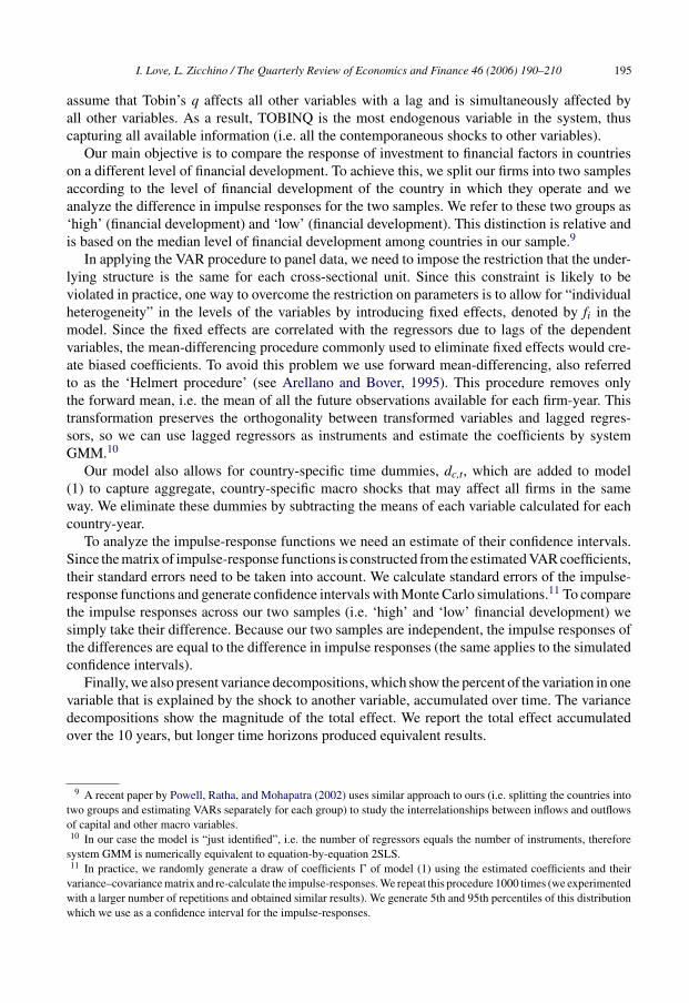
Table 1Sample coverage across countries

Country Countrycode

Number ofobservations

Percent of totalobservations

Number offirms

Financialdevelopment

Panel A: Low financial development sampleArgentina AR 250 0.005 39 −1.38Belgium BE 586 0.01 91 −0.82Brazil BR 894 0.02 143 −1.04Chile CL 507 0.01 74 −0.75Colombia CO 146 0.00 21 −1.6Denmark DK 1051 0.02 138 −0.49Finland FI 818 0.02 113 −0.41Indonesia ID 708 0.01 114 −1.17India IN 1856 0.03 294 −0.7Italy IT 1100 0.02 151 −0.64Mexico MX 522 0.01 76 −0.85New Zealand NZ 304 0.006 44 −0.53Philippines PH 406 0.008 68 −1.15Pakistan PK 546 0.01 88 −1.28Portugal PT 291 0.005 53 −0.67Sweden SE 1178 0.02 178 −0.31Turkey TR 248 0.005 54 −1.2Venezuela VE 92 0.002 13 −1.26

Group average 639 0.012 97 −1Group total 11503 1752

Panel B: High financial development sampleAustria AT 530 0.01 83 −0.27Australia AU 1383 0.03 184 0.42Canada CA 3136 0.06 443 0.03Switzerland CH 1087 0.02 151 2.2Germany DE 4092 0.08 582 1.68Spain ES 987 0.02 134 −0.14France FR 3338 0.06 524 0.1United Kingdom GB 8657 0.16 1165 1.68Israel IL 164 0.00 37 0.01Japan JP 6654 0.12 1271 3.3South Korea KR 1643 0.03 259 0.84Malaysia MY 1837 0.03 291 1.19Netherlands NL 1282 0.02 154 0.66Norway NO 878 0.02 148 −0.15Singapore SG 906 0.02 145 1.6Thailand TH 1233 0.02 185 0.36USA US 3399 0.06 356 1.35South Africa ZA 1189 0.02 244 0.25

Group average 2355 0.044 353 1Group total 42395 6356

Total sample 53898 8108

Countries are split into two groups based on the median level of financial development.


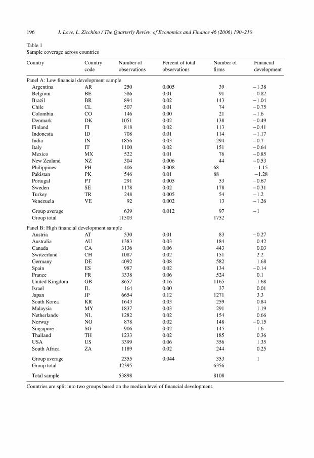
Table 2Variable definitions

Abbreviation Description

Firm-level variables (from Worldscope)CAPEX Capital expenditureNETPEQ Property plant and equipmentSALES Net sales or revenuesIKB Investment to capital ratio = CAPEX/(NETPEQ − CAPEX)SKB Sales to capital ratio = SALES/(NETPEQ − CAPEX)CF Cash flow (derived from Worldscope cash flow to sales ratio)CFKB Cash flow divided by (NETPEQ − CAPEX)RANK Ranking based on size of PPENT (first ranked by year, then averaged over the years), largest

firm in each country has rank equal to oneTOBINQ Tobin’s q, generated as market value of equity plus book value of total liabilities divided by

book value of total assets

Country-level variablesSTKMKT Stock market development is Index 1 from Demirguc-Kunt and Levine (1996), equals to the

sum of (standardized indices of) market capitalization to GDP, total value traded to GDP, andturnover (total value traded to market capitalization)

FININT Financial intermediary development is Findex1 from Demirguc-Kunt and Levine (1996),equals to the sum of (standardized indices of) ratio of liquid liabilities to GDP, and ratio ofdomestic credit to private sector to GDP

FD Financial development = STKMKT + FININTGDPPC GDP per capita from World development indicatorsHIGHINC World bank classification category based on 2002 gross national income per capita

2.1. Data

Our firm-level data come from the Worldscope database, which contains standardized account-ing information on large publicly traded firms and includes 36 countries with over 8000 firms forthe years 1988–1998. Table 1 gives the list of countries in the sample with the number of firmsand observations per country, while details on the sample selection are given in Appendix 1. Thenumber of firms included in the sample varies widely across the countries and the less developedcountries are underrepresented. The US and UK have more than 1000 firms per country, whilethe rest of the countries have only 136 firms on average (Japan is the third largest with over600 firms). Such a prevalence of US and UK companies might overweight these countries in thecross-country regressions and prevent smaller countries from influencing the coefficients.12

We constructed the index of financial development, FD by combining standardized measuresof five indicators from Demirguc-Kunt and Levine (1996): market capitalization over GDP, totalvalue traded over GDP, total value traded over market capitalization, ratio of liquid liabilities(M3) to GDP and credit going to the private sector over GDP. We split the countries into twogroups based on the median of this indicator. We refer to these two groups as ‘high’ (financialdevelopment) and ‘low’ (financial development), but we remind the reader that this distinction

12 To reduce the influence of countries with a large number of firms we also run our regressions with a subgroup of firmsin each country, i.e. only including a fixed number of the largest firms. The inclusion criteria are based on firm ranking,where rank one is given to the largest firm in each country. The results obtained were very similar to the ones reported inthe paper and are available on request.


Table 3Summary statistics for main variables

Low financial development sample High financial development sample

Mean Standarddeviation

25thpercentile

50thpercentile

75thpercentile

Mean Standarddeviation

25thpercentile

50thpercentile

75thpercentile

SKB 3.39 3.54 1.06 2.31 4.38 4.12 4.05 1.41 2.92 5.33IKB 0.21 0.15 0.10 0.17 0.28 0.21 0.14 0.11 0.18 0.27CFKB 0.29 0.32 0.11 0.22 0.38 0.28 0.28 0.13 0.23 0.38TOBINQ 1.35 0.78 0.89 1.11 1.51 1.46 0.76 1.00 1.22 1.63

Summary statistics by country for main variables. Variable definitions are given in Table 2. Countries are split into two groupsbased on the median level of financial development.

is relative and is based on the median level of financial development among countries in oursample.

Table 2 summarizes all the variables used in the paper (note that we normalize all the firm-levelvariables by the beginning-of-period capital stock), and Table 3 reports the summary statistics forthe firm-level variables.

3. Results

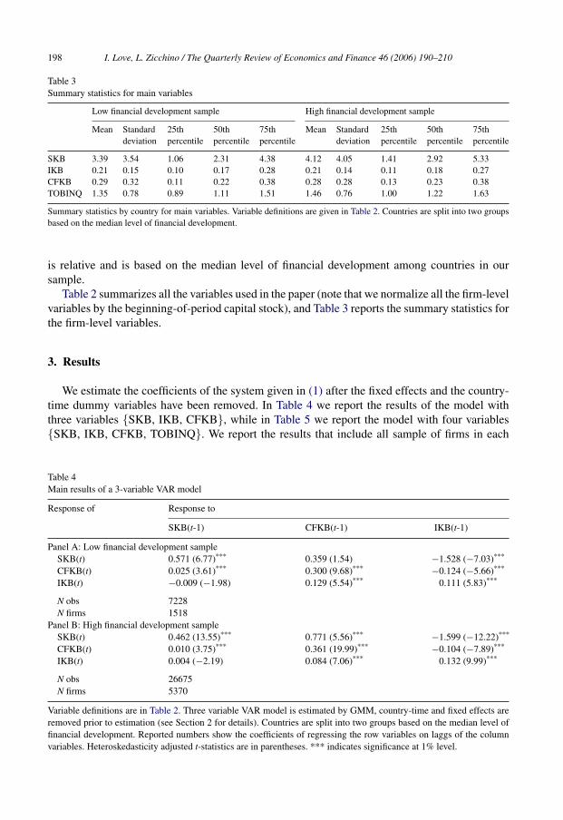
We estimate the coefficients of the system given in (1) after the fixed effects and the country-time dummy variables have been removed. In Table 4 we report the results of the model withthree variables {SKB, IKB, CFKB}, while in Table 5 we report the model with four variables{SKB, IKB, CFKB, TOBINQ}. We report the results that include all sample of firms in each

Table 4Main results of a 3-variable VAR model

Response of Response to

SKB(t-1) CFKB(t-1) IKB(t-1)

Panel A: Low financial development sampleSKB(t) 0.571 (6.77)*** 0.359 (1.54) −1.528 (−7.03)***

CFKB(t) 0.025 (3.61)*** 0.300 (9.68)*** −0.124 (−5.66)***

IKB(t) −0.009 (−1.98) 0.129 (5.54)*** 0.111 (5.83)***

N obs 7228N firms 1518

Panel B: High financial development sampleSKB(t) 0.462 (13.55)*** 0.771 (5.56)*** −1.599 (−12.22)***

CFKB(t) 0.010 (3.75)*** 0.361 (19.99)*** −0.104 (−7.89)***

IKB(t) 0.004 (−2.19) 0.084 (7.06)*** 0.132 (9.99)***


Variable definitions are in Table 2. Three variable VAR model is estimated by GMM, country-time and fixed effects areremoved prior to estimation (see Section 2 for details). Countries are split into two groups based on the median level offinancial development. Reported numbers show the coefficients of regressing the row variables on laggs of the columnvariables. Heteroskedasticity adjusted t-statistics are in parentheses. *** indicates significance at 1% level.


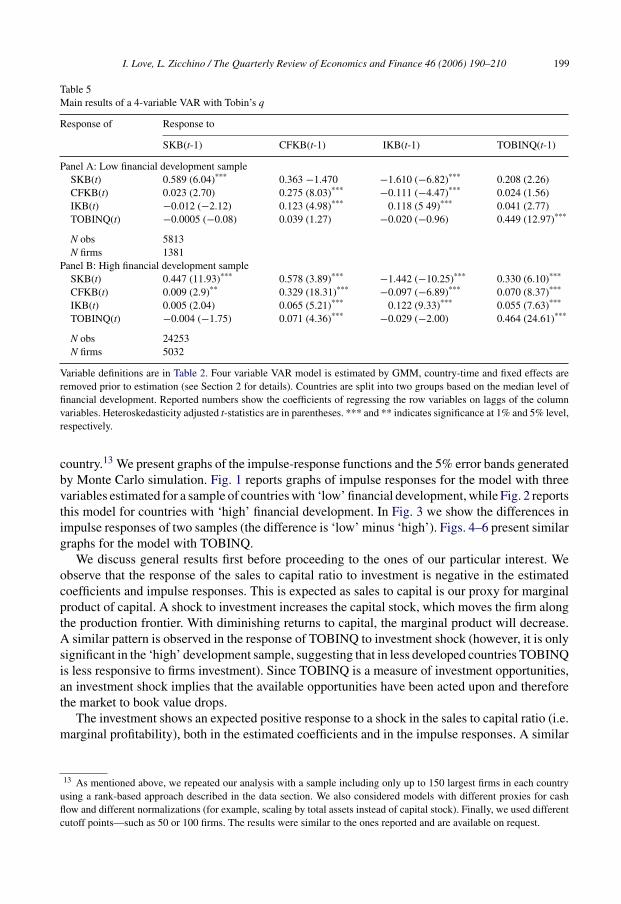
Table 5Main results of a 4-variable VAR with Tobin’s q

Response of Response to

SKB(t-1) CFKB(t-1) IKB(t-1) TOBINQ(t-1)

Panel A: Low financial development sampleSKB(t) 0.589 (6.04)*** 0.363 −1.470 −1.610 (−6.82)*** 0.208 (2.26)CFKB(t) 0.023 (2.70) 0.275 (8.03)*** −0.111 (−4.47)*** 0.024 (1.56)IKB(t) −0.012 (−2.12) 0.123 (4.98)*** 0.118 (5 49)*** 0.041 (2.77)TOBINQ(t) −0.0005 (−0.08) 0.039 (1.27) −0.020 (−0.96) 0.449 (12.97)***


Panel B: High financial development sampleSKB(t) 0.447 (11.93)*** 0.578 (3.89)*** −1.442 (−10.25)*** 0.330 (6.10)***

CFKB(t) 0.009 (2.9)** 0.329 (18.31)*** −0.097 (−6.89)*** 0.070 (8.37)***

IKB(t) 0.005 (2.04) 0.065 (5.21)*** 0.122 (9.33)*** 0.055 (7.63)***

TOBINQ(t) −0.004 (−1.75) 0.071 (4.36)*** −0.029 (−2.00) 0.464 (24.61)***


Variable definitions are in Table 2. Four variable VAR model is estimated by GMM, country-time and fixed effects areremoved prior to estimation (see Section 2 for details). Countries are split into two groups based on the median level offinancial development. Reported numbers show the coefficients of regressing the row variables on laggs of the columnvariables. Heteroskedasticity adjusted t-statistics are in parentheses. *** and ** indicates significance at 1% and 5% level,respectively.

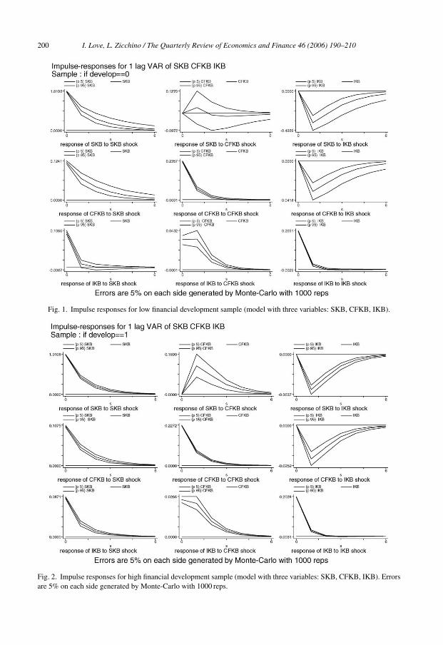
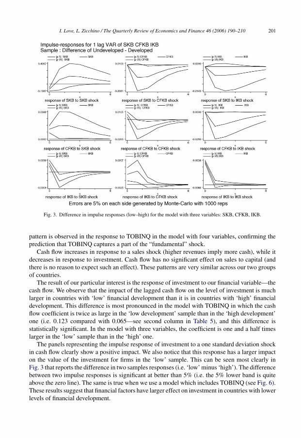
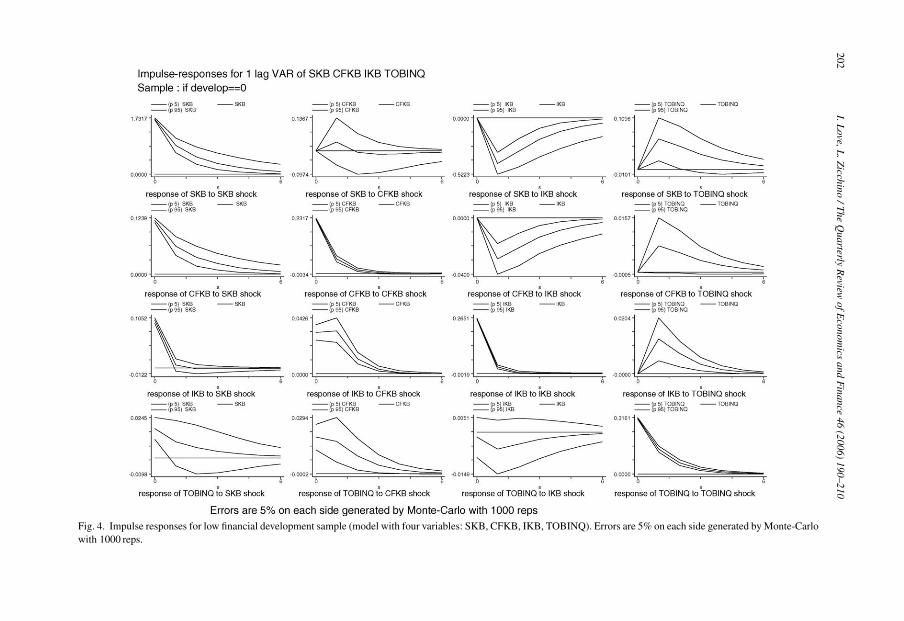
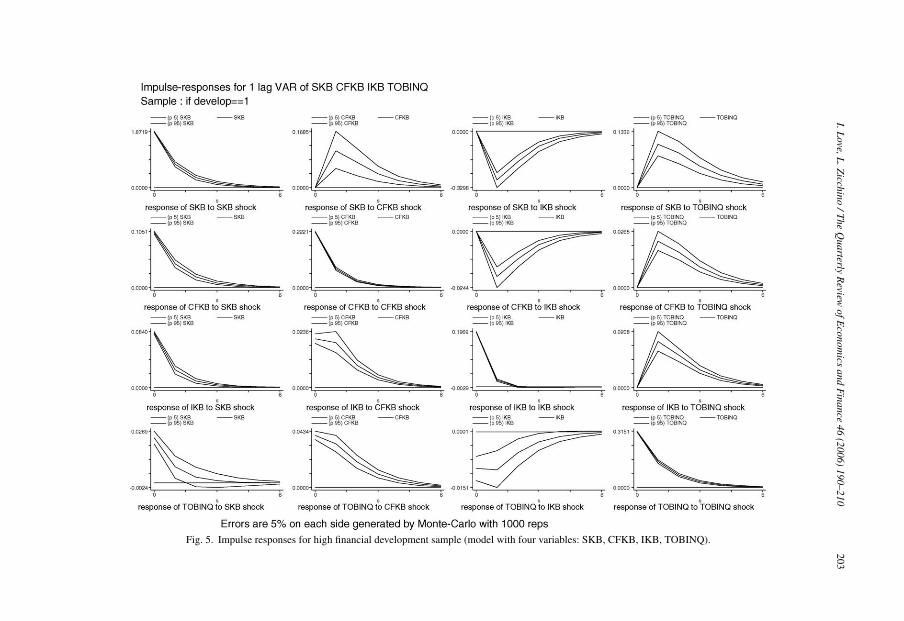
country.13 We present graphs of the impulse-response functions and the 5% error bands generatedby Monte Carlo simulation. Fig. 1 reports graphs of impulse responses for the model with threevariables estimated for a sample of countries with ‘low’ financial development, while Fig. 2 reportsthis model for countries with ‘high’ financial development. In Fig. 3 we show the differences inimpulse responses of two samples (the difference is ‘low’ minus ‘high’). Figs. 4–6 present similargraphs for the model with TOBINQ.

We discuss general results first before proceeding to the ones of our particular interest. Weobserve that the response of the sales to capital ratio to investment is negative in the estimatedcoefficients and impulse responses. This is expected as sales to capital is our proxy for marginalproduct of capital. A shock to investment increases the capital stock, which moves the firm alongthe production frontier. With diminishing returns to capital, the marginal product will decrease.A similar pattern is observed in the response of TOBINQ to investment shock (however, it is onlysignificant in the ‘high’ development sample, suggesting that in less developed countries TOBINQis less responsive to firms investment). Since TOBINQ is a measure of investment opportunities,an investment shock implies that the available opportunities have been acted upon and thereforethe market to book value drops.

The investment shows an expected positive response to a shock in the sales to capital ratio (i.e.marginal profitability), both in the estimated coefficients and in the impulse responses. A similar

13 As mentioned above, we repeated our analysis with a sample including only up to 150 largest firms in each countryusing a rank-based approach described in the data section. We also considered models with different proxies for cashflow and different normalizations (for example, scaling by total assets instead of capital stock). Finally, we used differentcutoff points—such as 50 or 100 firms. The results were similar to the ones reported and are available on request.


Fig. 1. Impulse responses for low financial development sample (model with three variables: SKB, CFKB, IKB).

Fig. 2. Impulse responses for high financial development sample (model with three variables: SKB, CFKB, IKB). Errorsare 5% on each side generated by Monte-Carlo with 1000 reps.


Fig. 3. Difference in impulse responses (low–high) for the model with three variables: SKB, CFKB, IKB.

pattern is observed in the response to TOBINQ in the model with four variables, confirming theprediction that TOBINQ captures a part of the “fundamental” shock.

Cash flow increases in response to a sales shock (higher revenues imply more cash), while itdecreases in response to investment. Cash flow has no significant effect on sales to capital (andthere is no reason to expect such an effect). These patterns are very similar across our two groupsof countries.

The result of our particular interest is the response of investment to our financial variable—thecash flow. We observe that the impact of the lagged cash flow on the level of investment is muchlarger in countries with ‘low’ financial development than it is in countries with ‘high’ financialdevelopment. This difference is most pronounced in the model with TOBINQ in which the cashflow coefficient is twice as large in the ‘low development’ sample than in the ‘high development’one (i.e. 0.123 compared with 0.065—see second column in Table 5), and this difference isstatistically significant. In the model with three variables, the coefficient is one and a half timeslarger in the ‘low’ sample than in the ‘high’ one.

The panels representing the impulse response of investment to a one standard deviation shockin cash flow clearly show a positive impact. We also notice that this response has a larger impacton the value of the investment for firms in the ‘low’ sample. This can be seen most clearly inFig. 3 that reports the difference in two samples responses (i.e. ‘low’ minus ‘high’). The differencebetween two impulse responses is significant at better than 5% (i.e. the 5% lower band is quiteabove the zero line). The same is true when we use a model which includes TOBINQ (see Fig. 6).These results suggest that financial factors have larger effect on investment in countries with lowerlevels of financial development.

202I.L

ove,L.Z

icchino/T

heQ

uarterlyR

eviewofE

conomics

andF

inance46

(2006)190–210

Fig. 4. Impulse responses for low financial development sample (model with four variables: SKB, CFKB, IKB, TOBINQ). Errors are 5% on each side generated by Monte-Carlowith 1000 reps.

I.Love,L

.Zicchino

/The

Quarterly

Review

ofEconom

icsand

Finance

46(2006)

190–210203

Fig. 5. Impulse responses for high financial development sample (model with four variables: SKB, CFKB, IKB, TOBINQ).

204I.L

ove,L.Z

icchino/T

heQ

uarterlyR

eviewofE

conomics

andF

inance46

(2006)190–210

Fig. 6. Difference in impulse responses (low–high) for the model with four variables: SKB, CFKB, IKB, TOBINQ. Errors are 5% on each side generated by Monte-Carlo with1000 reps.


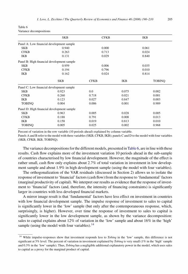
Table 6Variance decompositions

SKB CFKB IKB

Panel A: Low financial development sampleSKB 0.940 0.000 0.061CFKB 0.263 0.713 0.024IKB 0.131 0.029 0.840

Panel B: High financial development sampleSKB 0.959 0.006 0.035CFKB 0.194 0.796 0.010IKB 0.162 0.024 0.814

SKB CFKB IKB TOBINQ

Panel C: Low financial development sampleSKB 0.923 0.0 0.075 0.002CFKB 0.260 0.718 0.021 0.001IKB 0.123 0.027 0.847 0.003TOBINQ 0.004 0.006 0.001 0.989

Panel D: High financial development sampleSKB 0.963 0.005 0.028 0.005CFKB 0.188 0.791 0.008 0.013IKB 0.158 0.019 0.813 0.010TOBINQ 0.005 0.025 0.002 0.968

Percent of variation in the row variable (10 periods ahead) explained by column variable.Panels A and B refer to the model with three variables (SKB, CFKB, IKB); panels C and D to the model with four variables(SKB, CFKB, IKB, TOBINQ).

The variance decompositions for the different models, presented in Table 6, are in line with theseresults. Cash flow explains more of the investment variation 10 periods ahead in the sub-sampleof countries characterised by low financial development. However, the magnitude of the effect israther small, cash flow only explains about 2.7% of total variation in investment in low develop-ment sample and about 1.9% in high development sample (using the model with four variables).

The orthogonalization of the VAR residuals (discussed in Section 2) allows us to isolate theresponse of investment to ‘financial’ factors (cash flow) from the response to ‘fundamental’ factors(marginal productivity of capital). We interpret our results as evidence that the response of invest-ment to ‘financial’ factors (and, therefore, the intensity of financing constraints) is significantlylarger in countries with less developed financial markets.

A mirror image result is that ‘fundamental’ factors have less effect on investment in countrieswith low financial development sample. The impulse response of investment to sales to capitalis significantly lower in the ‘low’ sample (but only after the contemporaneous response, which,surprisingly, is higher). However, over time the response of investment to sales to capital issignificantly lower in the low development sample, as shown by the variance decomposition:sales to capital explains about 12% of variation in the ‘low’ sample and about 16% in the ‘high’sample (using the model with four variables).14

14 While impulse-responses show that investment responds less to Tobinq in the ‘low’ sample, this difference is notsignificant at 5% level. The percent of variation in investment explained by Tobinq is very small (1% in the ‘high’ sampleand 0.3% in the ‘low’ sample). Thus, Tobinq has a negligible additional explanatory power in the model, which uses salesto capital as a proxy for the marginal product of capital.

206I.L

ove,L.Z

icchino/T

heQ

uarterlyR

eviewofE

conomics

andF

inance46

(2006)190–210

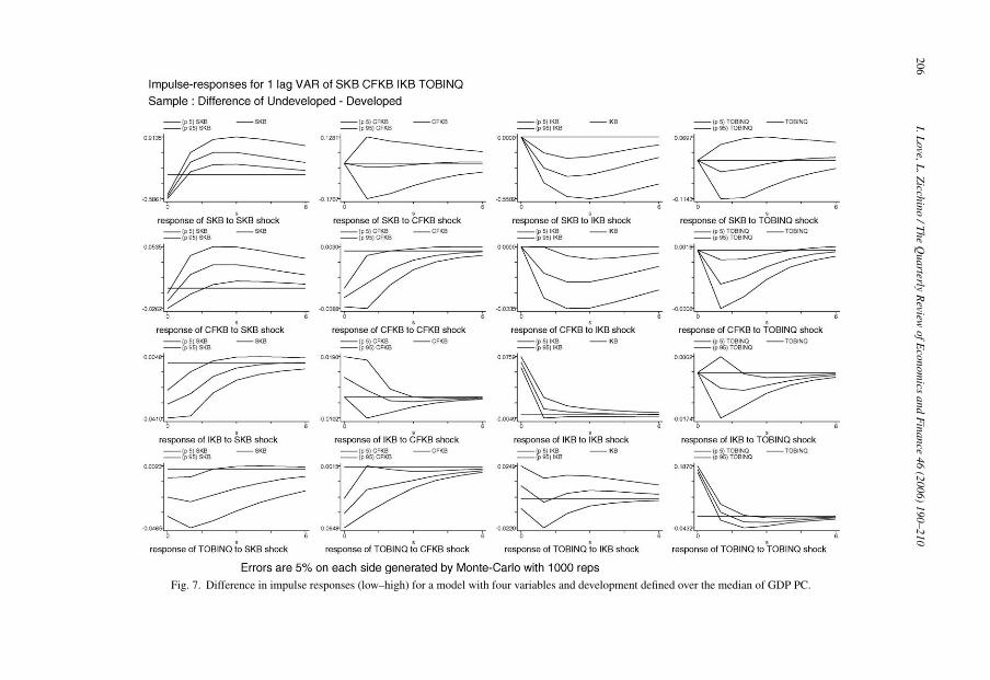
Fig. 7. Difference in impulse responses (low–high) for a model with four variables and development defined over the median of GDP PC.

I.Love,L

.Zicchino

/The

Quarterly

Review

ofEconom

icsand

Finance

46(2006)

190–210207

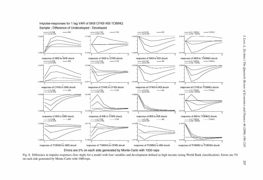
Fig. 8. Difference in impulse responses (low–high) for a model with four variables and development defined as high income (using World Bank classification). Errors are 5%on each side generated by Monte-Carlo with 1000 reps.


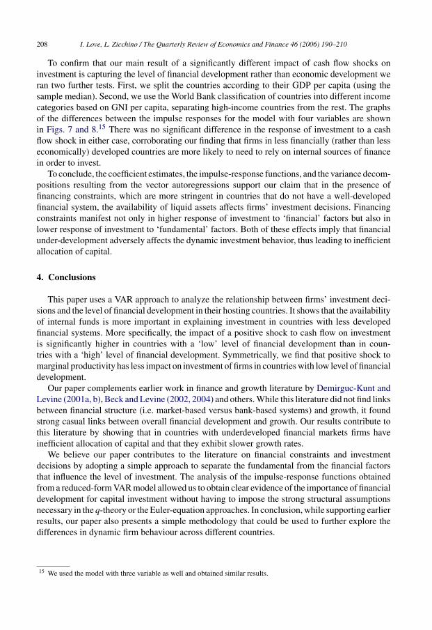
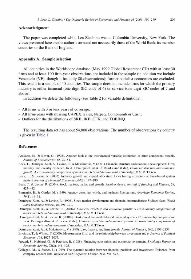
To confirm that our main result of a significantly different impact of cash flow shocks oninvestment is capturing the level of financial development rather than economic development weran two further tests. First, we split the countries according to their GDP per capita (using thesample median). Second, we use the World Bank classification of countries into different incomecategories based on GNI per capita, separating high-income countries from the rest. The graphsof the differences between the impulse responses for the model with four variables are shownin Figs. 7 and 8.15 There was no significant difference in the response of investment to a cashflow shock in either case, corroborating our finding that firms in less financially (rather than lesseconomically) developed countries are more likely to need to rely on internal sources of financein order to invest.

To conclude, the coefficient estimates, the impulse-response functions, and the variance decom-positions resulting from the vector autoregressions support our claim that in the presence offinancing constraints, which are more stringent in countries that do not have a well-developedfinancial system, the availability of liquid assets affects firms’ investment decisions. Financingconstraints manifest not only in higher response of investment to ‘financial’ factors but also inlower response of investment to ‘fundamental’ factors. Both of these effects imply that financialunder-development adversely affects the dynamic investment behavior, thus leading to inefficientallocation of capital.

4. Conclusions

This paper uses a VAR approach to analyze the relationship between firms’ investment deci-sions and the level of financial development in their hosting countries. It shows that the availabilityof internal funds is more important in explaining investment in countries with less developedfinancial systems. More specifically, the impact of a positive shock to cash flow on investmentis significantly higher in countries with a ‘low’ level of financial development than in coun-tries with a ‘high’ level of financial development. Symmetrically, we find that positive shock tomarginal productivity has less impact on investment of firms in countries with low level of financialdevelopment.

Our paper complements earlier work in finance and growth literature by Demirguc-Kunt andLevine (2001a, b), Beck and Levine (2002, 2004) and others. While this literature did not find linksbetween financial structure (i.e. market-based versus bank-based systems) and growth, it foundstrong casual links between overall financial development and growth. Our results contribute tothis literature by showing that in countries with underdeveloped financial markets firms haveinefficient allocation of capital and that they exhibit slower growth rates.

We believe our paper contributes to the literature on financial constraints and investmentdecisions by adopting a simple approach to separate the fundamental from the financial factorsthat influence the level of investment. The analysis of the impulse-response functions obtainedfrom a reduced-form VAR model allowed us to obtain clear evidence of the importance of financialdevelopment for capital investment without having to impose the strong structural assumptionsnecessary in the q-theory or the Euler-equation approaches. In conclusion, while supporting earlierresults, our paper also presents a simple methodology that could be used to further explore thedifferences in dynamic firm behaviour across different countries.

15 We used the model with three variable as well and obtained similar results.


Acknowledgment

The paper was completed while Lea Zicchino was at Columbia University, New York. Theviews presented here are the author’s own and not necessarily those of the World Bank, its membercountries or the Bank of England

Appendix A. Sample selection

All countries in the Worldscope database (May 1999 Global Researcher CD) with at least 30firms and at least 100 firm-year observations are included in the sample (in addition we includeVenezuela (VE), though it has only 80 observations); former socialist economies are excluded.This results in a sample of 40 countries. The sample does not include firms for which the primaryindustry is either financial (one digit SIC code of 6) or service (one digit SIC codes of 7 andabove).

In addition we delete the following (see Table 2 for variable definitions):

- All firms with 3 or less years of coverage;- All firm-years with missing CAPEX, Sales, Netpeq, Compnumb or Cash;- Outliers for the distributions of SKB, IKB, CFK, and TOBINQ.

The resulting data set has about 54,000 observations. The number of observations by countryis given in Table 1.

References

Arellano, M., & Bover, O. (1995). Another look at the instrumental variable estimation of error component models.Journal of Econometrics, 68, 29–51.

Beck, T., Demirguc-Kunt, A., Levine, R., & Maksimovic, V. (2001). Financial structure and economic development: Firm,industry, and country evidence. In A. Demirguc-Kunt & R. RossLevine (Eds.), Financial structure and economicgrowth: A cross-country comparison of banks, markets and development. Cambridge, MA: MIT Press.

Beck, T., & Levine, R. (2002). Industry growth and capital allocation: Does having a market- or bank-based systemmatter? Journal of Financial Economics, 64(2), 147–180.

Beck, T., & Levine, R. (2004). Stock markets, banks, and growth: Panel evidence. Journal of Banking and Finance, 28,423–442.

Bernanke, B., & Gertler, M. (1989). Agency costs, net worth, and business fluctuations. American Economic Review,79(1), 14–31.

Demirguc-Kunt, A., & Levine, R. (1996). Stock market development and financial intermediaries: Stylized facts. WorldBank Economic Review, 10, 291–321.

Demirguc-Kunt, A., & Levine, R. (2001a). Financial structure and economic growth: A cross-country comparison ofbanks, markets and development. Cambridge, MA: MIT Press.

Demirguc-Kunt, A., & Levine, R. (2001b). Bank-based and market-based financial systems: Cross-country comparisons.In A. Demirguc-Kunt & R. Levine (Eds.), Financial structure and economic growth: A cross-country comparison ofbanks, markets and development. Cambridge, MA: MIT Press.

Demirguc-Kunt, A., & Maksimovic, V. (1998). Law, finance, and firm growth. Journal of Finance, 8(6), 2107–2137.Erickson, T., & Whited, T. (2000). Measurement Error and the relationship between investment and q. Journal of Political

Economy, 108, 1027–1057.Fazzari, S., Hubbard, G., & Peterson, B. (1988). Financing constraints and corporate investment. Brookings Papers on

Economic Activity, 78(2), 141–195.Gallegati, M., & Stanca, L. (1999). The dynamic relation between financial positions and investment: Evidence from

company account data. Industrial and Corporate Change, 8(3), 551–572.


Gilchrist, S., & Himmelberg, C. (1995). Evidence on the role of cash flow for investment. Journal of Monetary Economics,36, 541–572.

Gilchrist, S. Himmelberg C. (1998). Investment, fundamentals and finance. NBER Working Paper 6652.Hamilton, J. (1994). Time series analysis. Princeton University Press.Hayashi, F. (1982). Tobin’s marginal q and average q: A neoclassical interpretation. Econometrica, 50(1), 213–224.Hubbard, G. (1998). Capital-market imperfections and investment. Journal of Economic Literature, 36(1), 193–225.Love, I. (2003). Financial development and financing constraints: International evidence from the structural investment

model. Review of Financial Studies, 16, 765–791.Powell, A., Ratha, D., & Mohapatra, S. (2002). Capital inflows and outflows: On their determinants and consequences

for developing countries. Mimeograph.Rajan, R. G., & Zingales, L. (1998). Financial development and growth. American Economic Review, 88(3), 559–586.Schiantarelli, F. (1996). Financial constraints and investment: Methodological issues and international evidence. Oxford

Review of Economic Policy, 70–89.Wurgler, J. (2000). Financial markets and allocation of capital. Journal of Financial Economics, 58(1–2), 187–214.Zicchino, L. (2001). Endogenous financial structure and business fluctuations in an economy with moral hazard. Mimeo-

graph: Columbia University.

Documents

Financial development and dynamic investment behavior ...siteresources.worldbank.org/DEC/Resources/...investment_Behaviour.pdf · Financial development and dynamic investment behavior: