Embed Size (px)
Citation preview

Financial Health Economics∗
Ralph S.J. Koijen† Tomas J. Philipson‡ Harald Uhlig§
February 2014
ABSTRACT
Many analysts argue that the expansion of the US health care sector is closely linked to
medical innovation and its demand. This paper provides the first explicit analysis of the
link between financial- and real markets for health care by considering how the returns
to medical R&D interacts with the growth of the sector. We document evidence of a
“medical innovation premium,” a large risk premium of about 4-6% annually higher than
is predicted by benchmark asset pricing models for firms engaged in medical R&D. We
interpret this premium as compensating investors for bearing government induced profit
risk on developed innovations and analyze its quantitative implications for the growth of
future health care spending. Our calibration implies substantial effects of the premium
on innovation and health care spending and therefore needs to be incorporated into any
future projections of the size of this sector. Removing government risk would almost
triple medical R&D spending, making it fall in line with the large value of health gains
estimated in the literature, and thereby increase health spending further by 4% of GDP.
∗First version: May 2011. We are grateful to Gary Becker, John Cochrane, Amy Finkelstein, John Heaton,Casey Mulligan, Jesse Shapiro, Amir Sufi, Stijn Van Nieuwerburgh, Pietro Veronesi, Rob Vishny, and Moto Yogoand seminar participants at Chicago Booth (finance workshop), “Hydra conference” on Corsica (2012), BonnUniversity, Columbia University, Humboldt University (Berlin), Federal Reserve Bank of Philadelphia, Whar-ton, the University of Chicago (applications workshop), Wharton, USC, Yale, TED-MED, and the AmericanEnterprise Institute for useful discussions and suggestions.
†Address: London Business School, Regent’s Park, London, NW1 4SA, United Kingdom, email: [email protected].
‡Address: University of Chicago, Harris School, Suite 112, 1155 E. 60th Street, Chicago, IL 60637, U.S.A,email: [email protected]
§Address: University of Chicago, Department of Economics, RO 325A, 1126 East 59th Street, Chicago, IL60637, U.S.A, email: [email protected]. This research has been supported by the NSF grant SES-0922550.

Improvements in health are a major component of the overall gain in economic welfare and
reduction in world inequality during the last century (Murphy and Topel (2006) and Becker,
Philipson, and Soares (2005)). Indeed, an emerging literature finds that the value of improved
health is on par with many other forms of economic growth as represented by material per-capita
income reflected in conventional GDP measurements. As such, the increase in the quantity and
quality of life may be the most economically valuable change of the last century. At the same
time, the current size of this sector, now close to a fifth of the US economy, and its continued
growth gives rise to concerned public debates.
Medical innovation and its demand are central to these improvements in health. Through
medical progress, including improvements in knowledge, procedures, drugs, biologics, devices,
and the services associated with them, there is an increased ability to prevent and treat old
and new diseases. Many analysts emphasize that this surge in medical innovation is key to
understanding the rapid expansion of the health care sector (Newhouse (1992), Cutler (1995),
and Fuchs (1996)).
To understand the growth of this sector, and the medical R&D that induces it, it is important
to understand the financial returns of those investing in medical innovation. This paper provides
a first, quantitative analysis of the joint determination of the financial returns of firms that
invest in medical R&D and the resulting growth of the health care sector.
We provide empirical evidence that the returns on firms in the health care industry are
substantially higher, around 4-6% per annum, than what is predicted by standard empirical
asset pricing models such as the Capital Asset Pricing Model (Sharpe (1964)) and the Fama
and French (1992) model. This large “medical innovation premium” suggests that the health
care industry may be exposed to risks that are not captured by these asset pricing models.
Our theoretical analysis then investigates the link between financial markets, incentives for
medical innovation, and the growth in the real health care sector. A standard asset pricing
1

perspective implies that the health industry risk premium should reflect an aggregate risk com-
ponent to which the health care industry is exposed in a particularly strong way. The premium
diminishes incentives for medical R&D, since the investments must recoup the higher returns
delivered to investors on average. Put differently, if the medical innovation premium could be
eliminated, we should observe more medical R&D. This provides a potential explanation for
the “missing R&D” implied by the analysis by Murphy and Topel (2006), which suggests that
the gains to health justify much larger investments in medical R&D than are actually observed.
Our theoretical analysis offers a potential explanation of the documented innovation pre-
mium and trace out its quantitative implications for the growth of the health care sector. We
interpret the premium to arise from one distinguishing feature of the health care sector: the
important role of the public sector in affecting profitability. We analyze the growth of the health
care sector when the risk that investors face is that the US government negatively affects the
returns to medical innovation whether through approval regulations or reimbursement risks that
threaten future markups.1 An illustration of such government risk affecting medical innovation
is the current slow down in investments due to the uncertain fate of US health care reform.
There are three major reasons why we consider government risk to be a plausible explanation
of the medical innovation premium. First, government greatly affects both the onset of profits
through approval regulations as well as the variable profits conditional on such approval. For
example, demand subsidy programs such as Medicare and Medicaid currently make up about
half of medical spending in the US, clearly an important component affecting the profits of
innovators. We argue that investors need be compensated for holding firms that engage in
medical innovation as they are exposed to these unique government shocks, resulting in a med-
ical innovation premium. Second, we seek an aggregate risk component, to which the health
sector is particularly exposed: government intervention risk in that sector has that property.
Third, we show that other plausible risk factors, such as for instance longevity risk, often imply
1See Ellison and Mullin (2001) and Golec, Hegde, and Vernon (2010) for an example around the Clintonhealth care reform.
2

a negative medical innovation premium in standard consumption-based asset pricing models,
which is the opposite of what we find empirically.
We model the government intervention as a one-time, low-probability switch of reducing
profits permanently. This is akin to creating a rare disaster to profits, from the perspective
of the innovators. The rare-disaster approach has been used in a number of recent papers
to explain equity premia, see for instance Barro and Ursua (2008), Barro and Jin (2011) or
Gabaix (2012). Here, the application is to the health industry specifically. Of course, what
may be a disaster from the perspective of the innovators may be beneficial for society as a
whole. We distinguish between the actuarially fair premium arising from the yet unobserved
intervention and the risk premium due to risk aversion against this event. In our calibrated
section, we show that the latter is the larger component. While the former induces an equity
premium regardless as to whether the intervention is idiosyncratic or common across firms,
the latter premium arises only due to a common, aggregate intervention risk. Furthermore, if
idiosyncratic risks are not “rare,” but rather represent the regular uncertain outcomes of R&D,
they will not give rise to risk premia, when investors hold a diversified portfolio. We therefore
focus entirely on rare aggregate interventions by the government.
We quantify the implications of the medical innovation premium stemming from government
risk using data on publicly traded firms engaged in medical R&D in the US from 1960 to 2010.
It is important to separate the firms that invest in medical R&D that expands the health care
sector from the service providers of care or the payers that insure such care. Our empirical
analysis applies to the former that are mainly device-, biologic-, and drug-manufacturers. The
providers delivering care are mainly hospitals, doctors, and nursing homes that are largely
non-profit or privately-held institutions.2 Payers or insurance companies are largely publicly
2For example, CMS data indicate that the three largest spending categories in 2010 were hospitals (31%),doctors (20%), nursing home and home care (14%) of which a small fraction is publicly traded. The annualAmerican Hospital Association survey for 2010 indicate that only 17% of the nation’s 5,754 hospitals are investor-owned, which includes both privately- and publicly-held hospitals. Although data on physician groups is notreadily available, the vast majority is believed to be privately held.
3

held as well, but our evidence suggests the medical innovation premium is not present for these
companies, consistent with an interpretation that such firms are not exposed, or not as much,
to government risk related to markups and approvals.
Using trends in health care spending, investment in medical R&D, and asset returns, we
calibrate the technology and preference parameters of our model. We use the model to study
two counterfactuals to assess the quantitative importance of the medical innovation premium
for the future growth of health care spending and investment in medical R&D.
The main result is that the medical innovation premium has large effects on future spending
on health care and medical R&D. More precisely, we first consider the case in which we remove
the risk premium, but preserve the impact on expected profits of government markup risk.
As government markup risk affects both expected cash flows and the discounting of firms, we
want to separate the two. We find that the size of the health care sector would increase by
4% of GDP if the risk premium is removed, and an additional 1% if the impact on expected
profits is removed as well. Hence, the largest impact of government intervention risk on health
care spending and investment in medical R&D is due to risk premia as opposed to changes in
expected profits.
In terms of impacting R&D spending, we find that it is almost three times as high in
the absence of the medical innovation premium. These large effects of the medical innovation
premium also have implications for the long-run health care share. By 2050, our model suggests
that 31% of GDP is spent on health care, conditional on no government intervention. The long-
run steady state share is slightly below 35% of GDP. The CBO projects that the total spending
on health care would rise from 16% of gross domestic product (GDP) in 2007 to 25% in 2025,
37% in 2050, and 49% in 2082. Hence, our model produces estimates for the health care share
that are somewhat lower than the CBO projections.
4

I. Related Literature and Institutional Background
A. Related Literature
Our paper relates to several strands of previous research by attempting to merge insights
from the three separate fields of health economics, macro-economics, and finance. It differs
from previous work in those fields by examining the joint determination of asset returns for
those investing in medical innovation and the resulting growth in the health care sector. In
these fields, one related literature discusses the relationship between health and growth, but it
does not analyze the returns to investing in medical R&D, see for instance Barro (1996) and
Sala-i-Martin, Doppelhofer, and Miller (2004). A large empirical literature, see Gerdtham and
Jonsson (2000) for a review, estimates the impact of economic growth on health care spending.
A seminal paper analyzing the interrelationship between macroeconomic growth and the
share of income spent on health is Hall and Jones (2007). These authors point out that a
rise in the share is predicted by many reasonable preference specifications, as additional health
spending increases longevity while the marginal utility for extra consumption declines with
growth. Hall and Jones (2007) provide a detailed quantitative analysis of the effect and social
desirability of health spending.3 We view our paper as complementary to theirs. In particular,
our focus is on the innovation in the health sector and the entrepreneurial risks associated with
that investment, while these authors assume technological progress in the health sector to be
deterministic and exogenous. While the long-run demand for new innovations in health may well
be due to the forces discussed by Hall and Jones (2007), the key entrepreneurial risks arise from
the possibility of governmental intervention rather than, say, risks in the effectiveness of health
spending in increasing longevity, as we discuss in Section VI. Compared to their model, our
3The empirical evidence showing that health care is a luxury good is mixed, see Acemoglu, Finkelstein, andNotowidigdo (2009) and the references therein. Also, in the cross-section, health care is a necessity in the upperpart of the income distribution, suggesting that technology may ultimately be the barrier to rich people fromspending larger shares of their incomes on health care.
5

model puts the incentives for R&D at center stage, which requires us to extend the model along
this dimension, while simplifying the longevity analysis performed by Hall and Jones (2007).
Our quantitative analysis thus complements their analysis by providing additional predictions
on the interaction of risk premia, R&D effort, and the rising share of health spending.
In finance, our paper relates to a recent literature that shows that government risk affects
asset prices. The main contribution of our paper is to document the medical innovation premium
in the health care sector and to map out the implications for investment in medical R&D and
health care expenditures. As a potential explanation of this risk premium, we point to the risk
of government intervention.
Belo, Gala, and Li (2013) link the cross-section of expected stock returns to firms’ exposures
to the government sector. Brogaard and Detzel (2013) use the political uncertainty index of
Baker, Bloom, and Davis (2013) to show that spikes in political uncertainty go together with
declines in the stock market, which is largely the result of increases in risk premia. Kelly,
Pastor, and Veronesi (2014) show how political uncertainty is priced in the option market using
national elections and global summits, building on the theory developed in Pastor and Veronesi
(2011) and Pastor and Veronesi (2012). These papers do not focus on the health care sector.
Most closely related to our paper are Ellison and Mullin (2001) and Golec, Hegde, and
Vernon (2010) who study the impact of the Clinton health care reform proposals in 1992 and
1993 on stock prices. Both papers find that health care stocks are negatively impacted by the
Clinton reform plans. Furthermore, Golec, Hegde, and Vernon (2010) also show that the effect
is more pronounced for R&D intensive firms and that (unexpected) R&D declines more for
those firms who are more exposed to government intervention risk. This evidence is consistent
with the main mechanism of our model.
Our empirical findings may have important implications for other questions in public finance,
6

and in particular the valuation of government programs such as Medicare and Medicaid. 4 Dis-
counting such liabilities using the Treasury curve may be inappropriate as these liabilities may
be exposed to the same risk as the health care sector as a whole, which implies that the discount
rate should reflect the medical innovation premium.
B. Institutional Background
Existing evidence suggests that a large share of health care spending growth is attributable
to technological change rather than increased demand for the same technologies over time. For
example, Newhouse (1992) provides calibrations that indicate that growth in aging, insurance,
or income does not explain a majority of the growth in health care spending suggesting that
technological change is likely a large contributor of the remaining share.
The technological change that raises health care spending comes from mainly from three
categories: medical devices, biologics, and drugs. In the US, the returns on these new tech-
nologies are determined both by private and public reimbursement policies. According to the
Centers for Medicare & Medicaid Services (CMS), in 2012 about 44% of US spending was
publicly financed, mainly through the Medicare and Medicaid programs. However, returns in
other parts of the world are more contingent on public reimbursement policies. For example, in
many European countries, roughly 85% of health care is publicly financed (OECD, 2013). For
drugs and biologics in the US, reimbursements can be paid directly to manufactures, such as in
the Medicaid drug program, or indirectly, through premium subsidies in the Medicare Part D
program for outpatient drugs. However, for devices, reimbursements are often indirect through
reimbursements to providers, for instance, through the Medicare diagnosis-based payments to
hospitals (DRGs) in the US that cover the use of a given device for a certain diagnosis.
The time and cost of bringing these new medical technologies to the market can be sub-
4See Geanakoplos and Zeldes (2011) and Lucas (2010) for recent work on the valuation of governmentliabilities.
7
stantial. For drugs and biologics, DiMasi and Hansen (2003) find that for 68 randomly selected
new drugs of 10 pharmaceutical firms, the average cost was about $802 million (2000 dollars).
This cost includes the cost of failures in the FDA approval process as only 12% of products
that enter the process actually make it to market (DiMasi and Hansen 2003).
New health care products are often discovered by academic research. One may argue that
investment decisions by such institutions are not driven by the future earnings of the products.
However, the high cost of development of medical products requires outside investors, whose
main focus is on (risk-adjusted) earnings. Hence, even though the “R” in medical R&D may
not be motivated entirely by future returns, the “D” certainly is. Indeed, drugs and biologics
are among the most R&D intensive industries in the US as measured by R&D to sales ratio
of about 16% (PhRMA (2013)) compared to a 2.8% share of US GDP being devoted to R&D
(Robbins, Belay, Donahoe, and Lee (2012)).
To raise capital for these large development costs, manufacturers often use public capital
markets. It is important to note that much of the production of goods and services in health
care are not financed through public equity markets, even though medical innovation largely is.
Providers of hospital services, making up about a 35% of health care spending, are about 70%
not-for profit and thus rely on debt or donations instead of public equity. Physician services,
making up an additional 22% of health care spending (CMS 2012), are often organized in small
privately-financed clinics. Given the lack of public equity financing in these major health care
sectors, it is understandable that for-profit firms engaged in medical innovation makes up a
large majority of the firms listed on public exchanges.
Government policies in the US disproportionally affect the returns on medical R&D invest-
ments as world sales for medical products is highly concentrated in the US. Egan and Philipson
(2013) use data from the World Bank and WHO to estimate that US health care spending was
about 48% of world spending in 2012 even though US GDP was only about 24% of world GDP
in the same year. For biopharmaceutical spending, the US share of world spending is lower at
8
about 39%, as many emerging markets spend a larger share of their overall health care on bio-
pharmaceuticals (Egan and Philipson (2013)). Given the larger markups on US spending, most
profits are generated on US markets. Because of the concentration of world profits in the US,
changes in reimbursement policies that threaten US markups is of primary importance to those
investing in medical R&D. We therefore focus on the risk of U.S. government reimbursement
policies on asset prices.
II. Empirical Evidence: The Medical Innovation Premium
A. Data
We use data from various sources. Information on overall health care spending comes
from the National Health Expenditure Accounts from the Centers for Medicare and Medicaid
Services. International data on health expenditures to GDP and the data on pharmaceutical
expenditures are from the OECD Health Data 2010.
We use data on industry returns, the Fama and French factors, and market capitalization
from Kenneth French’s website. The first classification we use splits the universe of stocks
in five industries: “Consumer goods,” “Manufacturing,” “Technology,” “Health care,” and a
residual category “Other.” The health care industry includes medical equipment, 5 pharma-
ceutical products,6 and health services.7 We also study the 48 industry classification, which
splits the health care industry into the three aforementioned categories. We follow the industry
classification as on Ken French’s website for both the entire health care industry and for the
three sub-industries.
5The corresponding SIC codes are 3693: X-ray, electromedical app., 3840-3849: Surgery and medical instru-ments, 3850-3851: Ophthalmic goods.
6The corresponding SIC codes are: 2830: Drugs, 2831: Biological products, 2833: Medical chemicals, 2834:Pharmaceutical preparations, 2835: Invitro, in vivo diagnostics, and 2836: Biological products, except diagnos-tics.
7The corresponding SIC codes are 8000-8099: Services - health.
9
B. Risk Premia in Health Care Markets
We first study the returns of firms in the health care industry. In computing the returns
to health care companies, we correct for standard risk factors to account for other sources of
systematic risk outside of the model. Therefore, we are interested in the intercepts, or “alphas,”
of the following time-series regression:
rt − rft = α + β ′Ft + εt,
where Ft is a set of risk factors. We are interested in the returns of health care firms relative
to firms that are not in the health care industry. To compute the relative returns, we regress
the returns on a constant, the alpha, and a set of benchmark factors, Ft. The alpha measures
the differential average return of health care firms that cannot be explained by standard asset
pricing models.
Asset pricing models are distinguished by the pricing factors Ft they account for. As a first
model, we use the excess return on the CRSP value-weighted return index, which is comprised
of all stocks traded at AMEX, NYSE, and Nasdaq. This is a common implementation of the
Capital Asset Pricing Model (CAPM), see Sharpe (1964). The second benchmark asset pricing
model we consider is the 3-factor Fama and French (1992) model, which is labeled “Fama-
French.” In addition to the market factor, this model also accounts for firm size (the “SMB”
factor) and the value factor (the “HML” factor). Empirically, smaller firms and firms with
high book-to-market ratios, that is, value firms, tend to have higher average returns that are
not explained by difference in CAPM betas. These additional two factors account for these
regularities in asset markets.8
8There is a large literature that provides explanations for the size and value effects, see for instance Berk,Green, and Naik (1999), Zhang (2005), Yogo (2006), Lettau and Wachter (2007), and Koijen, Lustig, and VanNieuwerburgh (2012). In this paper, we are particularly interested in the risk premium in the health careindustry above and beyond the standard risk factors and do not provide an explanation for the market, size,and value risk premia or exposures.
10

We present our main results for annual returns, using the Fama and French model, and for
the sample from 1961 to 2012, which is the period for which we observe health care spending.
The results are reported in Panel A of Table I. The first number corresponds to the alpha;
the second number is the t-statistic using OLS standard errors. We find that the health care
industry tends to produce economically and statistically significant alpha of 5.0% (with a t-
statistic of 2.4) relative to the Fama and French model.
We also report the alphas of the other industries and find that they do not have large alphas
relative to the standard models. We conclude that there is a risk premium for holding health
care stocks that cannot be explained by standard asset pricing factors.
If we remove health services and focus on medical equipment and pharmaceutical products,
the alphas are even higher at 6.4% and 5.4% per annum, respectively. This is because the
alphas on medical services are close to zero, which lowers the overall alpha of the health care
sector.9 Both alphas are statistically significant at conventional significance levels.
Although both sub-sectors, that is, medical equipment and drugs, earn significant alphas,
this is not necessarily driven by exposures to the same risk factor. To test this more directly,
we augment the Fama and French model with the health care factor and report the alphas in
Panel B of Table I. We find that the alphas are economically and statistically close to zero once
the health care factor is included in the model. This suggests that a similar risk determines the
mispricing relative to standard models in both sub-sectors.
Our results are consistent with the findings in Fama and French (1997), who study the
performance of the Fama and French (1992) model for a large cross-section of 48 industries.
Their Appendix B shows that the model is rejected in particular due to two industries: the
real-estate and the health-care industries. Despite the large and growing literature on returns
in real estate markets, little is known about health care markets.
9The returns on services start only in the late sixties, and we therefore exclude them from the table. However,their returns are well explained by standard models and the alphas are close to zero.
11

For robustness, we estimate the model also at a monthly frequency and for two additional
sample periods, namely from 1927 to 2012 and from 1946 to 2012. The first sample period is
the longest sample available. The second sample focuses on the post-war period. Furthermore,
we compute the alphas not only relative to the Fama and French model, but also relative to the
CAPM. The results for monthly returns and other sample periods are reported in the Online
Appendix, but the results are broadly consistent with the findings reported in Table I. If we
use monthly data, or longer sample periods, the statistical significance of the alphas increases
further.
Given the trends in health expenditures, as summarized in the Online Appendix, it is
interesting to study the trends in market capitalization of health care firms. Figure 1 plots the
share of all publicly-traded equity that is part of the health care industry. The figure shows
that the health care industry becomes an increasingly important share of publicly-traded equity.
If we look at the relative contributions of medical equipment (“devices”) and pharmaceutical
products (“pharma”), we find that firms working on pharmaceutical products make up the vast
majority of market capitalization.
It is important to point out that trends in shares of market capitalization do not mechanically
imply positive alphas. In fact, if we look at the change in shares across all 48 industries from
1945-2010, then we find that the change in market share and alphas are virtually uncorrelated
across industries. The market share of an industry may increase not only due to exceptional
returns on existing companies, but largely due to new companies going public. In support
of this argument in case of the health care sector, we do not find that the average firm size
increases more in the health care industry than in other industries.
12

C. Government Risk and the Health Care Sector
In this section, we provide new evidence on the importance of government risk on the
profitability and asset prices of health care firms, which extends the existing finance literature
that highlights the importance of government risk for asset prices, see Section I.
Risk Factors Identified from 10-K filings
Our first piece of new evidence comes from a text-based analysis of 10-K reports that each
firm files annually with the Securities and Exchange Committee (SEC). 10-K filings have been
explored recently in the finance literature to define industries (Hoberg and Phillips (2011)), to
measure competition (Feng Li and Minnis (2013)), to predict the volatility of stock returns (Ko-
gan, Levin, Routledge, Sagi, and Smith (2009)), and to predict future stock returns (Loughran
and McDonald (2011)). We show that a particular section of the 10-K filings may be helpful
to identify risk factors to which a firm is exposed. Our approach may have applications well
beyond this paper as understanding risk exposures of firms is central in both macro-economics
and finance.
We use the most recent 10-K filings that are available as of December 2013. In each 10-K
filing, there is a section 1.A labeled “Risk Factors.” The guidelines for this section are described
in Regulation S-K, Item 503(c) as:
Where appropriate, provide under the caption “Risk Factors” a discussion of the most sig-
nificant factors that make the offering speculative or risky. This discussion must be concise and
organized logically. Do not present risks that could apply to any issuer or any offering. Explain
how the risk affects the issuer or the securities being offered. [...] The risk factors may include,
among other things, the following:
1. Your lack of an operating history;
2. Your lack of profitable operations in recent periods;
13

3. Your financial position;
4. Your business or proposed business; or
5. The lack of a market for your common equity securities or securities convertible into or
exercisable for common equity securities.
To illustrate the data we use in this section. we include the “Risk Factors” section of the
10-K filings of Pfizer and Apple, which are among the largest health and non-health care firms
by the end of our sample, in the Online Appendix.
As is clear from the headings already, various forms of government regulation are a major
concern to Pfizer, while for Apple traditional risk factors such as economic conditions and
competition are more relevant. Moreover, in the spirit of our model, Pfizer explicitly mentions
price controls and government intervention as one of the key risk factors that may affect the
firm’s operations.
To illustrate that the pattern in the 10-K filings is more general and not particular to just
Apple and Pfizer, we hand-collect the sections on risk factors for the largest 50 health care
companies and the largest 50 non-health care companies. For each firms, we count the number
of times words related to the government or government risk appear in the filings.
The dictionary that we use is summarized in Table II. The dictionary attempts to capture
the prevalence of government-related risks in the 10-K filings. In the main dictionary, we avoid
words that are government-related yet particular to the health care sector such as “FDA.”
The results are summarized in Panel A of Table III. For firms in the health care sector,
we find that words in this dictionary appear on average 139 times, compared to on average 77
times for firms outside the health care sector. The standard error of the difference in means
equals 15.1, implying that the difference is statistically highly significant with a t-statistic of
4.1.
14

However, the typical 10-K filings for health care stock is longer. As an alternative measure,
we can look at the average fraction of words that appear in our dictionary. For firms within
the health care sector, this fraction is 1.51% while it is only 1.23% for firms in the non-health
care sector, implying that words from our dictionary appear 23% more frequently for firms in
the health care sector. If we again test on the difference in means, the standard error equals
0.099%, which implies once more that the difference is significant with a t-statistic of 2.8.
In our main dictionary, we omit government-related words from our dictionary that are
particular to the health care sector. We also explore how our results are affected if we include
the health care-specific terms “medicare,” “medicare reform,” “medicaid,” “medicaid reform,”
“ppaca,” “cms,” “healthcare reform,” “nhs,” and “fda” in our dictionary. The results for this
expanded dictionary are reported in Panel B of Table III. The differences in the average word
count and the average fraction increase substantially, making the differences economically and
statistically even more significant.
Taken together, the text-based analysis of 10-K filings provides shows that government risk
is an important concern for firms in the health care sector.
The cross-section of health care betas and event returns around Clinton’s health care reforms
Ellison and Mullin (2001) and Golec, Hegde, and Vernon (2010) show that health care stocks
decline around the Clinton reform in the early nineties. These events provide the best test of
our theory as the key component of the reform was to impose price controls on new drugs.
We extend the evidence in these papers in two ways. First, we show that firms in the health
care sector that have more negative cumulative abnormal returns around the major event dates
tend to have higher betas with respect to the health care factor. This result is important as
different exposures to the health care factor measure different exposures to the risk factor that
is not well priced by the CAPM and the Fama and French model and results in the large alphas
we document in Section II. Differences in exposures to the health care factor relate to differences
15

in abnormal returns around news about government intervention, we argue that government
risk is an important candidate determinant of the medical innovation premium we document
in this paper.10 Second, we consider a much larger cross section of firms. Ellison and Mullin
(2001) and Golec, Hegde, and Vernon (2010) select only 18 and 111 companies, respectively.
Our sample includes somewhat over 300 firms in the drugs, devices, and services sector.
As a starting point, it is useful to illustrate how important the discussions surrounding the
Clinton reform were for stock prices of health care firms. In Figure 2, we plot the drawdowns
for the health care sector alongside the drawdowns of the aggregate stock market. Drawdows
are defined as:
Dt =t∑
u=1
ru − maxs∈{1,...,t}
s∑
u=1
ru, (1)
where rt denotes the log return on either the aggregate stock market or the health care sector. 11
Hence, drawdowns measures the cumulative downturn relative to the highest level the indexed
reached up to a certain point in time. Drawdowns are a common way to identify risk in
investment strategies (see for instance Grossman and Zhou (1993), Landoni and Sastry (2013),
and Koijen, Moskowitz, Pedersen, and Vrugt (2013)).
Figure 2 points to three large downturns for the health care sector during the last two
decades: in the early nineties, during the 2000-2002 technology crash, and during the 2007-
2008 financial crisis. During the latter two periods, the drawdowns of the market are even
larger than those for the health care sector, reflecting the fact that the health care sector has
a beta below one.
The drawdown in 1992 and 1993 is of most interest to us, which coincides with the discus-
sions around the Clinton health care reform. During this period, the aggregate stock market
10Ideally, we would like to use alphas of individual firms directly, but those turn out to be to noisy. As betasare estimated more precily than alphas, we use betas with respect to the health care factor instead.
11For comparability, we scale both returns by the standard deviation of returns over the full sample.
16

increased, while the health care sector shows a large decline.
The graph indicates substantial negative effects of proposed Clinton reforms compared to
proposed and enacted Obama reforms. Hult and Philipson (2012) discuss an interpretation of
this result. They stress that government expansions often lower both demand prices (premiums
or copays) to raise access, but also at the same time cut supply prices (reimbursements) through
government monopsony power. Their analysis implies that R&D returns may rise when govern-
ment expansions include poorer parts of the population by raising quantity more than lowering
markups. For example, Medicaid expansions raise innovative returns in this manner. However,
innovative returns fall when expansions include richer parts of the population when markups
may fall more than quantity rises. For example, the single-payer European payment systems
may lower innovative returns in this manner. The non-monotonic impact of government expan-
sions across the income distribution implies that Clinton reforms may affect innovative returns
differently than Obama reforms. Clinton proposed population wide reforms including the entire
income distribution which may lead to negative innovation effects. This is in contrast to Obama
reforms, which was centered on raising access of the poor through Medicaid expansions and
exchange subsidies which thus may raise innovative returns.
We analyze stock prices during the Clinton reform in more detail and highlight the impor-
tance of political risk. Ellison and Mullin (2001) and Golec, Hegde, and Vernon (2010) identify
the key event dates during the Clinton reform proposals, which we reproduce in Table IV.
Our key objective is to show that firms that have higher health care betas measured over
periods much longer than the Clinton reforms, experience also much more negative returns
during these events. This implies that firms that are more sensitive government intervention
have higher health care betas with respect to the health care factor, which generates abnormal
returns relative to standard asset pricing models.
To this end, we first compute the health care beta by regressing monthly excess returns of
17

a given firm on the market return and the health care factor. This provides us the exposure to
the health care factor for each firm. The typical sample to estimate the beta is much longer
than the period over which Clinton care was discussed. As follows from Table V, the average
number of years used to estimate the beta is around 20 years.
Next, estimate the cumulative abnormal returns. We use an event window that spans from
5 days before until 5 days after the event. We use 250 daily returns prior to the event window
to estimate the betas relative to the CAPM model. If a firm has missing daily returns, it is
omitted from the sample.12 We then compute the cumulative abnormal return by aggregating
the residual from this regression (Campbell, Lo, and MacKinlay, 1997). We then sum over all
event dates to get the total impact of the Clinton reform proposal on each health care stock.
We then relate the overall risk exposure of health care firms, estimated over a much longer
sample on average, to the cumulative abnormal return during the events in 1992 and 1993
through a cross-sectional regression across firms:
CARi = δ0 + δ1βHC
i
σ (βHCi )
+ ui, (2)
where σ(βHC
i
)is the standard deviation of health care betas across firms. The coefficient δ1
measures how the cumulative abnormal return, CARi, changes if the beta with respect to the
health care factor, βHCi , changes by one standard deviation.
The main results are presented in Table V. Firms with higher health care betas are more
sensitive to news about future government intervention. A 1-standard deviation increase
in the health case beta corresponds to a 7.7% lower cumulative abnormal return. Using
heteroscedasticity-consistent standard errors, the effect is significant with a t-statistic of -2.7.
As a point of reference, the average cumulative abnormal return across all firms is -23.9%. The
R-squared of the regression equals 4%, which illustrates that abnormal returns are noisy, which
12This is only the case for 6 firms. Replacing the missing returns with the market return and subsequentlyincluding these firms, does not affect any of our results.
18
is to be expected.
Taken together, these results imply that firms with high exposures to the health care fac-
tor, which earns the medical innovation premium, are more sensitive to news about future
government intervention.
III. A Dynamic Model of Medical Innovation and Spending
In this section, we build a dynamic model to study the interaction between the risk premia
in the health care industry, investment in medical R&D, and medical spending.
A. The Environment
A.1. Preferences and Endowments
Time is infinite, t = 0, 1, . . .. There are two types of infinitely-lived households: “normal” or
“non-entrepreneurial” households i ∈ [0, 1] and “entrepreneurial” households or (more briefly)
entrepreneurs i ∈ (1, 1 + κ] for some κ > 0. We shall think of the latter is constituting a small
fraction of the entire population, i.e., we shall think of κ being small. We focus on symmetric
allocations and equilibria, with a representative household for each type.
Normal households have Cobb-Douglas preferences over health and non-health care con-
sumption:
U = E
∞∑
t=0
βt
(cξnth
1−ξnt
)1−η
1 − η
, (3)
where cnt is the non-health care consumption of a normal household at date t, hnt is the health
care consumption, η > 1 is the coefficient of relative risk aversion, β ∈ (0, 1) the time discount
factor, and ξ ∈ (0, 1) determines the trade-off between health care and non-health consumption.
19

Cobb-Douglas preferences imply that the marginal utility of consumption increases in health,
which is consistent with the empirical results in Viscusi and Evans (1990), Finkelstein, Luttmer,
and Notowidigdo (2008), and Koijen, Van Nieuwerburgh, and Yogo (2011).
We do not introduce life-extending benefits of health care or medical care, although one
can understand the benefits of health as enhancing the utility from regular consumption in the
preference specification above. The life-extending benefits are an important element of this
literature, see for instance Hall and Jones (2007). One could introduce them here as well. As
we discuss in section VI, longevity risk considerations are not a plausible candidate to generate
the observed risk premium for the medical sector, though. For that reason and in order to focus
on our main theme, we have abstract from the longevity issue here.
Normal households are endowed with one unit of time each period, which they supply
inelastically as labor. The productivity of labor for producing consumption goods is growing
exogenously with γ > 1. Households are further endowed with a base level of health, given
by hγt for some parameter h > 0, and thus assumed to be growing at the same rate as labor
productivity.
For entrepreneurs e, we abstract from health care consumption as well as labor supply. We
think of these as rich households, for which labor income does not matter much, whose labor
supply does matter much in the aggregate, and who purchase the best medical care available, but
which nonetheless constitutes only a small fraction of their income. We therefore concentrate
entirely on their consumption ce,t and, below, their asset holdings. Their preferences are given
by their value function
Ue,t = V (ce,t, Et[Ue,t+1]) . (4)
All that we really need below is the stochastic discount factor process Mt resulting from these
20

preferences. We assume that the preferences are piecewise linear and given by
Ue,t = u(ce,t) + βeEt [Ue,t+1] (5)
u(ce,t) =
θ(ce,t − c) for ce,t ≤ c
ce,t − c for ce,t ≥ c
for ce,t ≥ 0 and parameters βe, c, θ ≥ 1. This kinked-linear specification can be viewed as a
simple version of prospect theory, as in Kahneman and Tversky (1979). There are many other
preference specification that could serve just as well, as we discuss in a Online Appendix to this
paper.
A.2. Technologies and Feasibility
Let ct = cnt + κcet and ht = hnt denote aggregate non-health and health care consumption
at date t. The production of aggregate consumption ct is given by
ct = γtLct, (6)
where Lct are the total units of labor devoted to producing consumption goods. We use the
consumption good at time t as numeraire.
Health is produced according to the production function
ht = hγt
︸︷︷︸Exogenous health
+ mt︸︷︷︸Health due to medical care
, (7)
where hγt is the base health level the household is endowed with and mt is medical care,
an input to increase the health level beyond the base health level. One may wish to impose
some upper bound h̄γt as the maximal level of health that can be reached with state-of-the-art
medical care, in order to motivate our assumption above of abstracting from medical care for
21

entrepreneurial households.
Medical care is produced from a continuum of individual types, indexed by j ∈ [0, 1],
mt =
(∫ κ
0
m1/φjt dj
)φ
, (8)
where φ > 1. As is standard in models of monopolistic competition, φ determines the degree
of competition in the industry and hence the market power of producers in the competitive
equilibrium below.
The production of mjt units of type-j medical care is given by
mjt = qjtγtLmjt,
where Lmjt is the total units of labor used for producing type-j medical care, γt is the general
productivity increase, and qjt is the productivity or quality level for producing type-j medical
care relative to producing the consumption good. Therefore, q−1jt is also the marginal cost for
producing mjt in terms of the consumption good at time t. The evolution of the quality is given
by
qj,t+1 =(qνjt + dν
jt
)1/ν, (9)
where ν ≤ 1 is a parameter, and djt is the amount of R&D invested in the type-j-knowledge
qjt, created with labor per
djt = γtLdjt,
where Ldjt is the total labor used for undertaking type-j R&D, and γt is the general level of
productivity. We drop the j-subscript to denote aggregates. We shall focus on symmetric
22

equilibria, so that qt ≡ qjt, et cetera. Aggregate feasibility requires
Lct + Lmt + Ldt = 1. (10)
B. Government, Markets and Equilibrium
B.1. Government and Government Risk
We assume that the government intervenes in three ways that all affect the health care
sector. First, it proportionally subsidizes R&D undertaken by the firm, so that firms only need
to privately pay for a fraction 1 − χ of the costs of R&D, for some 0 < χ < 1. We keep this
level of subsidy fixed throughout. Second, it proportionally subsidizes the purchases of medical
care by households, so that households only pay for a fraction (1 − σ) of the market price of
medical care, for some 0 < σ < 1. We keep this level of subsidy fixed throughout.
Third, the government may restrict the prices firms can charge for medical care. We assume
that this restriction may randomly change over time: indeed, the main risk factor we consider
is this government price intervention risk. Without government intervention, firms act monop-
olistically competitive, which implies that prices equal marginal cost times a constant markup,
pt = φ/qt. However, with probability ω ∈ [0, 1], the government intervenes and caps markups
that firms can charge. In this case, the government imposes price controls and health care
prices are limited to pt = ζ/qt, where ζ ∈ [1, φ). For simplicity, we consider a one-time switch
that is permanent. We introduce a state variable zt that equals zero if the government has not
yet intervened, and one thereafter. We denote the markup at time t by μt = ztζ +(1− zt)φ and
therefore prices by pt = μt/qt. The economy thus starts from non-intervention, and finds itself
in the non-government intervention epoch, until the intervention happens. The probability that
zt = 1 converges to one as time converges to infinity.
23

Only the first two types of intervention create a flow of payments from the government, so
that the government budget constraint is given by
σptmt + χdt = τt + κτt,e, (11)
where τt are the lump sum taxes collected from normal households at time t and τt,e are the
lump sum taxes collected from entrepreneurial households at time t. We assume that the taxes
of each type of household pays for the subsidies received by that type of household,
σptmt = τt,
χdt = κτt,e.
Lump sum taxes and infinitely lived households imply Ricardian equivalence, provided we do
not also redistribute between households: we may therefore assume without loss of generality
that there is no government debt.
B.2. Firms
We assume that medical care and goods are traded on markets. We assume that each
period t, a new continuum of firms j ∈ [0, 1] is created by the entrepreneurs and owned by the
entrepreneurs, one for each type of medical care type. A firm is given a one-period patent for
developing the type-j medical technology and a monopoly for providing it in the next period.
The level of technology achieved is then made freely available to a new next firm created.
Taking into account the government risk, and dropping the sub-index j, a firm in period in
period t maximizes the firm value vt given by:
vt = maxdjt
Et (Mt+1πt+1) − (1 − χ)dt,
24

where Mt+1 is the stochastic discount factor of the entrepreneurs between period t and t + 1,
where (1−χ) reflects net costs for doing R&D after the government subsidy, and where πt+1 are
the date-(t + 1) profits of firm j created at date t. These profits are obtained in monopolistic
competition against all other firms present for the other types of medical care, subject to the
potential markup restriction by the government.
B.3. Households
We assume that normal households neither trade assets on financial markets nor hold shares
in firms. They receive labor income. They receive medical care purchase subsidies from the
government and pay taxes. They therefore maximize the utility U given by (3) by choosing cnt
and mt, subject to (8) and the sequence of budget constraints
cnt + (1 − σ)
∫ 1
0
pjtmjtdj + τt = γt, (12)
taking prices pjt for medical care of type j at date t as well as the medical care purchase subsidy
σ as given. The maximization problem of the households implies an aggregate demand function
Dj,t+1 (pj,t+1) for medical care of type j.
Entrepreneurs create new firms, pay for their costs arising from R&D, and receive income
from profits generated by the firms, which they have created in the previous period. They
maximize (4) subject to the sequence of budget constraints:
cet + τt,e + (1 − χ)1
κdt =
1
κπt. (13)
Note the division of R&D expenses and profits by κ, in order to properly “distribute” the
continuum j ∈ [0, 1] of firms over the “small” continuum j ∈ [1, κ] of entrepreneurial households.
25
B.4. Equilibrium
We focus on symmetric equilibria where all normal households make the same choices, all
entrepreneurs make the same choices, and where all firms make the same choices. Given the
exogenous process zt, an equilibrium is an adapted stochastic sequence
Ψ = (Mt, ct, mt, ht, ct,e, mt,e, ht,e, τt, Lct, Lmt, qt, dt, Ldt, pt, πt, vt, Dt (∙))∞t=0,
with qt measurable at t−1, such that households maximize their utility, given prices, government
interventions, and firm choices, entrepreneurs maximize utility, resulting in consumption ce,t and
the stochastic discount factor process Mt, firms maximize profits and value per setting their
own price, given prices set by other firms, wages, the stochastic discount factor and government
intervention, and markets clear.
IV. Model Solution and Implications
A. Health Care Demand
The budget constraint of the entrepreneurs as well as the government budget constraint
implies
κct,e = πt − dt, (14)
so that consumption of the entrepreneurial households is current period profits minus the ex-
penses for creating the next generation of firms. With the preferences given in (5), the stochastic
26

discount factor Mt+1 is
Mt+1 =
βe if ct,e > c, ct+1,e > c,
βe/θ if ct,e < c, ct+1,e > c,
θβe if ct,e > c, ct+1,e < c,
βe if ct,e < c, ct+1,e < c.
(15)
Profit maximization with monopolistic competition leads to the usual markup pricing over
marginal costs, subject to government intervention,
pt = μt/qt, (16)
where
μt =
φ if zt+1 = 0,
ζ if zt+1 = 1.(17)
The resulting profits are
πt =μt − 1
qt
mt. (18)
Total demand for health care is obtained from the intra-temporal optimization problem of
the households,
maxmt
(cξth
1−ξt
)1−η
1 − η, (19)
subject to the household budget constraint (12) as well as (7). This is solved by:
mt =
(1 − ξ
1 − σ
)(γt − τt
pt
)
− ξhγt, (20)
27

where pt is given by (16).
Let ϕt = ptmt/γt be the share of gross labor income spent by (normal) households on
medical care. Note that τt = σptmt = σϕtγt. With this, rewrite (20) as
ϕt =
(1 − ξ
1 − σ
)
(1 − σϕt) − ξhpt
and solve for ϕt. We find that the share evolves as
ϕt =ptmt
γt=
1 − ξ
1 − σξ−
1 − σ
1 − σξξhpt. (21)
The model has two important implications. First, if firms do not undertake any R&D, that
is, dt = 0, then qt and hence pt do not fluctuate over time, holding markups constant. Hence,
medical spending share increases only due to medical R&D, which lowers prices. Second, and
absent government intervention, the long-run share equals (1 − ξ)/(1 − σξ), and therefore
increases with the importance of health in the utility function (1 − ξ) and the size of the
subsidy in the output market (σ).
Upon intervention by the government, private incentives to undertake R&D collapse. As-
suming that the government does not directly finance R&D or organizes this industry in some
other way, the quality of medical care remains constant from the intervention point onward.
The price pt for medical care drops from μt/qt to 1/qt due to the elimination of the markup.
Equation (21) then implies an increase of the gross income share ϕt spent on medical care
in the period of the intervention, due to this price drop and its effect on valuing the health
endowment h. From there onwards, the gross income share ϕt remains constant, and will be
bounded above by (1−ξ)/(1−σξ). If the government finds a way to continue R&D indefinitely,
the quality qt may continue to grow to infinity, and the long-run share ϕt once again converges
to (1 − ξ)/(1 − σξ).
28

B. Optimal Medical R&D
Aggregate profits are
πt = xt(μt − 1). (22)
Consider a single firm j, choosing some R&D level djt, resulting in qj,t+1 =(qνt + dν
jt
)1/ν.
Suppose the R&D choices of all other firms result in the aggregate state of medical knowledge
qt+1. The standard monopolistic competition formulas imply
πjt =
(qjt
qt
)1/(φ−1)
πt,
The value maximization problem of the firm can therefore be written as
maxdt≥0
Et
[(qj,t+1
qt+1
)1/(φ−1)
Mt+1πt+1
]
− (1 − χ)djt,
s.t. qj,t+1 =(qνjt + dν
jt
)1/ν,
taking as given the aggregate variables qt, qt+1, Mt+1 and πt+1, and qt+1 known at date t. In
case of an interior solution, the first-order condition is
1 − χ =
(qνjt + dν
jt
)1/ν−1dν−1
jt
qt+1(φ − 1)
(qj,t+1
qt+1
) 1φ−1
−1
Et (Mt+1πt+1) . (23)
Imposing symmetry yields
1 − χ =dν−1
t
qνt + dν
t
1
φ − 1Et (Mt+1πt+1) ,
which can be solved for dt, if qt and Et (Mt+1πt+1) are known.
This equation illustrates how the risk premium we document in Section II slows down the
investment in medical R&D. The left-hand side of equation (23) measures the marginal cost of
29

investing in medical R&D and the right-hand side measures the marginal benefit. The marginal
benefit is lowered if Et (Mt+1πt+1) is lower. Expected returns of health care companies are given
by:
Et (Rt+1) =Et (πt+1)
Et (Mt+1πt+1), (24)
which implies:
Et (Mt+1πt+1) =Et (πt+1)
Et (Rt+1). (25)
We find in Section II that the expected returns on health care companies tend to be higher
than suggested by standard asset pricing models, which according to (25) lowers the discounted
value of profits and per (23) the incentives to invest in medical R&D.
V. Calibration and Quantitative Implications
In Section A, we discuss the stochastic discount factor, Mt. In Section B, we discuss how we
calibrate the model’s parameters, and provide intuition for how parameters are identified. We
then use the model in Section C for two counterfactuals. First, we consider the case in which
the government risk is removed all together (ω = 0). Second, we consider the case in which the
government risk is still present (ω > 0), but the stochastic discount factor is uncorrelated with
government risk. We conclude this section by studying the long-run implications of the model
in Section D.
A. Risk Preferences and the Stochastic Discount Factor
30

Given the preference specification (5) and the resulting stochastic discount factor (15),
we shall assume (or calibrate) c so that the entrepreneurial consumption ct,e during the non-
government intervention epoch is above this treshold for all t ≥ 0, and falls below it in the
period following a government intervention. In our calculations below, ct,e grows in the non-
intervention scenario, so that we simply need c < c0,e. Furthermore, in our benchmark govern-
ment intervention, markups and profits are shrunk to zero, so that entrepreneurial consumption
falls to zero: we then just need c > 0.
With that, the stochastic discount factor Mt+1 during the non-government intervention
epoch can be rewritten as
Mt+1 = R−1MHt+1, (26)
where
R = 1/Et[Mt+1] =1
βe (1 − ω + ωθ)(27)
is the rate of discounting that is not particular to the health care risk. In a model with standard
productivity shocks et cetera, R ought to reflect the risk pricing of such shocks. It is rather
straightforward to extend our preference specification and model to account for other risk factors
such as the aggregate stock market risk or even the Fama-French factors. However, to focus on
the economic mechanism at work, we restrict attention to the government risk factor only.
The second component of the stochastic discount factor, MHt+1, satisfies
1 = Et[MHt+1] (28)
and is the component that is specific to the health care sector, which in our model corresponds
31

to the risk of government intervention. With our assumption regarding c, it can be written as
MHt+1 =
M , if Δzt+1 = 1,
M , if Δzt+1 = 0 and zt = 0,
1 , if zt = 1,
where M > M and solve
M =θ
1 − ω + ωθ(29)
M =1
1 − ω + ωθ(30)
Per (28), note that
1 = (1 − ω)M + ωM (31)
Once the government intervenes (zt = 1), MHt+1 = 1 and risk premia in the health care sector
can be explained by standard risk factors. The fact M > M implies that when the government
intervenes, the marginal utility of wealth of the agent pricing the assets is high. This covariance
of marginal utility and profits generates a positive risk premium for health care firms that is
not accounted for with the traditional risk factors used in standard asset pricing models.
While we have derived this stochastic discount factor from the preference specification (5),
the latter is not essential: only the properties of the stochastic discount factor above matter
for the solution of the model. We could have thus alternatively started with assuming these
properties of Mt+1 and then reverse-engineer entrepreneurial preferences, which give rise to this
stochastic discount factor. For the kinked-linear preference specification in (5), it is easy to
solve for βe and θ, given ω, M , M and R, satisfying (31), from equations (27) and (29), but the
reverse-engineering approach can be applied to a wider variety of utility specifications, which
would thus serve just as well. We explore this route in a Online Appendix to this paper.
32

The simple form of the stochastic discount factor and the binary nature of the government
intervention risk allow for a particularly simple way of solving the model, while respecting key
nonlinearities elsewhere in the model during the convergence phase to the steady state.
B. Moments, Parameters, and Sensitivity
We need to calibrate the following set of parameters:
Θ ={γ, h, ν, q0, M, M, φ, ξ, ζ, χ, σ
}. (32)
The parameters β and η have no implications for medical innovation or spending decisions and
therefore do not need to be calibrated. We calibrate the model to five periods of 10 years
starting in 1960. Thus, t = 0 corresponds to 1960 and t = 5 corresponds to 2010. For the
calibration we shall additionally impose that zt = 0, t = 0, . . . , 5, which corresponds to no
government intervention.
In the model, we label γt the labor income of the normal households, whereas total output
is given by
yt = (1 + κ)γt + πt,
and includes the profits of health-care companies. To compare this equation to the data, it is
reasonable to think of yt as income from a growing stock of capital and labor that can be spent
on consumption and health care, that is, as gross domestic product net of gross investment.
Furthermore, profits of health care companies are a small share of GDP, so it is reasonable to
equate (1 + κ)γt with GDP net of gross investment.
Based on data from the St. Louis Fed, we set γ so that output growth equals 3.0% per annum,
that is, γ = 1.35. The profitability of health care firms is given by (ptmt − mt/qt)/(ptmt) =
(μt − 1)/μt. For the period in which the government did not intervene, zt = 0, profitability
33
equals (φ−1)/φ. Caves, Whinston, and Hurwitz (1991) show that prices of drugs fall by 80% if
a patent of a drug expires and generic drugs become available. This suggests φ = 5. However,
other expenses, such as marketing costs, decline as well after patent expiration, which suggests
a lower number. As a starting point, we therefore set φ = 3.
We then turn to the subsidy on medical care and medical R&D. According the the CMS,
about 50% of aggregate health care spending occurs via Medicare and Medicaid. We therefore
set σ = 50%. Further, we set the R&D subsidy to χ = 2, which roughly matches Jones (2011).13
In calibrating government intervention risk, we initially consider the case in which govern-
ment intervention reduces health care prices to marginal costs. This implies ζ = 1. We set the
probability of government intervention to ω = 10%, which implies that the probability that the
government did not intervene in a 50-year period equals 59%. We also explore the implications
for our main results of changing ω from ω = 10% to ω = 20%.14
Next, we calibrate the stochastic discount factor. R is the relevant discount rate in the
absence of government intervention risk. For the arguments given in McGrattan and Prescott
(2003), we set R equal to 4% per annum, or R = 1.48 in our model in which a period corresponds
to a decade. To calibrate MHt+1, we first note that, using the assumptions made before:
E(πt+1)
E(πt+1Mt+1)= RM−1. (33)
We think of R as the return coming from the CAPM or the Fama-French model. M−1 is the
medical innovation premium that we estimate to be around 4-6% per year, and we calibrate to a
baseline return R of 4% as discussed above and an additional risk premium of 5%. We therefore
set RM−1 = 1.0910 = 2.37. Also, given our assumptions made previously, M no longer affects
13The ratio of private to public medical R&D spending increased in the last decade, which may also justify alower value of χ.
14One may wonder whether our alpha could simply be a Peso problem. For a 4% alpha per year, the per-yearprobability of intervention would be ωA = 1 − 1.05−1. To probability of no intervention for a 60-year periodthen equals 1.05−60 = 5%, which is rather unlikely.
34

spending or R&D decisions.
We select the remaining four parameters, h , ν, q0, and ξ to match the R&D share in 1990
and 2010, as well as the health share in 1960 and 2010. We use data on health care spending
from the CMS and data on R&D spending is from Jones (2011).
We illustrate the fit of the model relative to the data in Figure 3. In Table VI we summarize
the model parameters for ω = 10% as well as ω = 20%.
C. Risk Premia, Medical Innovation, and Medical Spending
To understand the impact of government intervention risk and risk premia on health care
spending and investment in medical R&D, we proceed in two steps. First, we remove all
government risk. Removing government risk altogether has two effects. On the one hand,
there is no risk premium effect anymore. On the other hand, the expected profits of firms
engaged in medical R&D increase. To separate both effects, we also consider the case where
the government risk is still present, but there is no risk premium effect. By comparing both
counterfactuals, we can assess the cash flow and discount rate effects separately.
C.1. First Counterfactual: No Government Risk
The first counterfactual we consider is when all government risk is removed, that is, ω = 0.
Since there is no risk, the stochastic discount factor takes the same value in both states, that
is, Mt+1 = R−1. The results are presented in Figure 4. The solid line presents the benchmark
case. The dotted line corresponds to the case in which we remove government risk altogether.
The figure applies to the no-government intervention epoch.
In the absence of government risk, the discount rate firms apply to medical R&D investments
is lower and the expected profits are higher. As such, medical R&D rises more rapidly. By 2010,
35

the R&D share almost triples the R&D share in the presence of risk premia and government
risk.
As a result of medical R&D, the price of medical care falls and the health care share rises
more rapidly as well. The impact is quantitatively large as the share of GDP spent on medical
care rises from about 20% to 25% in 2010 in this counterfactual scenario.
If we use the calibration corresponding to ω = 20%. The results are presented in Table VII.
Even though the R&D share rises somewhat more rapidly in this case, the effect is quantitatively
small. We conclude that changing ω and re-calibrating the model has a minor effect on this
counterfactual.
C.2. Second Counterfactual: No Government Risk Premium
As a second counterfactual, we consider the case in which the government risk is present
(ω = 10%), but we set the price of government intervention risk to zero, M = M = 1. This
case corresponds to the dashed line in Figure 4. This case allows us to understand two effects
that are in play in the first counterfactual separately. More precisely, if all government risk
is removed, then Et(πt+1) increases and the price of this cash flow, Et(Mt+1πt+1), increases
as well. We are particularly interested in the effect of risk premia on medical innovation and
spending, and therefore want to hold constant the impact on expected profits, Et(πt+1).
Based on Figure 4, we see that the discount rate effect is the main driver of the increased
health care and R&D share. Even holding expected profits constant, the health share would
increase to 24.5% and the R&D share would increase to 1.9%.
If we use the calibration corresponding to ω = 20%. The results are presented in Table VII.
It follows that the main conclusions are not very sensitive to the level of government risk.
36
The main insight of both counterfactuals is that accounting for government can lead to
different conclusions on spending and innovation trends. Comparing the second to the first
counterfactual highlights that the results are mostly driven by the presence of a risk premium
as opposed to an effect on expected cash flows.
D. Long-Run Implications
Absent government intervention, the long-run health care share implied by the model equals
(1−ξ)/(1−σξ), which equals 36% in the presence of subsidies. If subsidies in the output market
are removed, that is, σ = 0, the share increases to only 22%. Figure 5 illustrates the evolution
of the health care spending share and the R&D share as implied by the model, provided no
government intervention takes place. Obviously, the convergence is rather slow and the health
care share is expected to increase to 31% by 2050. This prediction is similar to the model of
Hall and Jones (2007).
For alternative assumptions about government risk, the long-run health share increases to
35% for ω = 20%. Hence, the long-run implications of our model are fairly independent of the
amount of government risk.
Once the government intervenes, R&D activity will come to a halt, if left to private markets.
The R&D share drops to zero, the gross income share ϕt spent on medical care jumps, but then
remains constant, as explained below equation (21).
37

VI. Mechanisms for Health Care Risk Premia
A. Broad Intuition for Alternative Mechanisms
In this section, we discuss various economic mechanisms that may give rise to a positive risk
premium in the health care industry. This boils down to understanding how certain shocks,
in general equilibrium, co-move with the investors’ marginal utility. This is meant as an ex-
ploratory exercise, not some all-encompassing theory. Simply put, some approaches throw up
harder challenges than others. This section uses a broad theory brush to discuss how and why,
focussing on the key economic arguments and without providing a comprehensive list of assump-
tions and caveats. We first provide a broader overview, and then examine some approaches in
somewhat more careful detail.
The key insight from the empirical asset pricing results is as follows. Given the positive
health industry alphas, it should be the case that ∂U/∂ct+1 is low when health industry profits
πt+1 are high.Ceteris paribus, marginal utility is low if consumption is high.
Consider a representative household that demands medical care m, resulting in health h =
m. Medical care can be provided with productivity (or “quality”, “inverse of marginal costs”)
q, and sold at price p, subsidized at rate σ. The subsidies are financed per lump-sum taxes τ on
the household. Assume a linear production function and denote the markup with φ. Profits of
the medical sector are π. Aggregate income is y, while aggregate consumption is c. Preferences
by the household are given by a utility function u(c, h).
For a linear production function, the relationship between prices, marginal costs, mark-ups
and profits are:
p =φ
qand π = (φ − 1)
h
q. (34)
38

The household budget constraint is:
y + π = c + (1 − σ)ph + τ. (35)
The government budget constraint is:
σph = τ. (36)
Together, we obtain the following two key equations:
c = y − h/q = y − π/(φ − 1), (37)
π = (φ − 1)h/q. (38)
These equations imply that approaches that treat y, φ, q as parameters or constants are chal-
lenging to pursue. Consider the following sources of uncertainty:
1. Medical progress, including longevity: see subsection B for more elaboration. If q in-
creases, so will h.
2. Preference shocks for h, with c and h separable or complements in the utility function
u(∙, ∙).
3. A shock to the subsidies σ.
The challenge is the following. Suppose that these shocks result in surprise increases in profits
π. They will then lead to lower consumption. Conversely, lower profits go together with higher
consumption. In the cases above, this should yield a negative, not a positive alpha.
Approaches which treat all of π, h, c, y, φ, q as endogenous have more potential to be suc-
cessful. Consider the following sources of uncertainty:
1. Medical progress and productivity. Suppose a surprise increase in q leads to a more
39

productive workforce, thereby increasing y. It is then possible, in principle, to have both
π and c increase.
2. A preference shock for h, where c and h are (strong) substitutes in the utility function
u(∙, ∙). Suppose that h is increased and thus profits π increase, while consumption c
decreases. In principle, it is nonetheless possible that the marginal utility of consumption
decreases as well.
3. Government regulatory risk regarding φ: if φ declines unexpectedly, then so will π and c,
while h increases.
These approaches face challenges on their own. The first one may not be sufficient quantita-
tively: while medical progress has perhaps led to somewhat longer working life and to fewer
absentee hours due to sickness in the US after the Second World War, these effects may be too
small to sensibly generate the medical innovation premium that we estimate in our empirical
work. The second approach may not be plausible. Per own introspection, it does seem to
us that consumption, and marginal increases thereof, are more fun and not less fun, if one
is healthy.15 We therefore chose the third approach as the key approach in this paper. The
arguments above are painted with a broad brush: it is entirely conceivable, even plausible,
that reasonable exceptions can be found that allow the pursuit of other alternatives. For some
of them, more detail is useful to reveal where the challenges lie exactly. We shall do so in
particular for longevity risk.
B. Risk Premia Due to Longevity Effects
Longevity is the key to understanding the growth of health expenditures in the model of
Hall and Jones (2007). Our paper is not in contrast to theirs; rather, it is complementary.
15This is also with the empirical results in Viscusi and Evans (1990), Finkelstein, Luttmer, and Notowidigdo(2008), and Koijen, Van Nieuwerburgh, and Yogo (2011).
40

While longevity may indeed be key (and indeed, our long-run improvements in health may well
be interpreted as increases in longevity), we argue here that they are unlikely to be the risk
factor giving rise to the medical innovation premium.
Consider a three-period extension of the model above, t = 0, 1, 2, where the household surely
survives until t = 1. The probability of survival from t = 1 to t = 2 depends on health, f (h1),
where f ′ (h1) > 0. The household’s problem can then be summarized by:
max(h1)
u (c0) + βE0 [u (c1)] + β2E0 [f (h1) u (c2)] , (39)
where the maximization is subject to the resource constraints, yt + πt = ptht + ct, the prices
of medical care, pt = φt/qt, and firm profits, πt = ht (φt − 1) /qt.16 Unless noted otherwise, we
focus on shocks to qt that lower the marginal cost of producing medical care.
Optimal period-1 health follows from max(h1) u (c1) + f (h1) b, where b = βE1 [u (c2)] > 0 a
constant. In this case, we have c1 = y1−h1q−11 = y1−(φ1 − 1)−1 π1, which implies that consump-
tion and profits are negatively correlated. Since M1 = βu′ (c1) /u′ (c0) = βu′(y1 − (φ1 − 1)−1 π1
)/u′ (c0),
profits and the stochastic discount factor are positively correlated. This implies a negative risk
premium for health care firms. This holds true regardless of the survival function f (h1) and as
long as u′ (c) < 0.
VII. Conclusion
Despite the fact that improvements in health have been a major component of the overall
gain in economic welfare during the last century, the continued incentives for medical innovation
and the resulting growth of the health care sector are not well-understood. In particular,
16Relative to our full model, we consider a simpler production for health with h= 0 and ν = 1, which impliesthat medical spending maps one-to-one to health, mt = ht.
41

although it is generally believed that technological change through medical innovation is a
central component of the expansion of this sector, little is known about what risks affect the
returns of these R&D investments and how those risks affect future spending growth in health
care.
We provided an empirical and theoretical analysis of the link between asset markets and
health care spending. We first documented a “medical innovation premium” for the returns of
medical R&D firms in the US during the period 1960 to 2010. The excess returns relative to
standard risk-adjustments were estimated to be between 4-6% per annum, which is non-trivial
and about the same size as other asset pricing puzzles such as the equity risk premium and
the value premium during this period. Motivated by this finding, we provide a first theoretical
analysis of the joint determination of financial and real health care markets, analyzing the joint
behavior of medical R&D returns in asset markets and the growth of the real health care sector.
We interpret the medical innovation premium to result from government markup risks that
may require investors to demand higher returns on medical R&D investments beyond standard
risk-adjusted returns. We simulated the quantitative implications of our analysis and found
that there would have been a sizeable expansion of the health care sector, on the order of 7%,
in absence of this government risk.
Our analysis raises many future research questions that need to be addressed to more fully
understand the growth of health care sectors around the world. First, if government uncertainty
discourages health care R&D, then how are standard analyses of government interventions al-
tered taking into account of this effect? For example, most governments across the world
attempt to stimulate medical R&D through various push and pull mechanisms. But if the
government uncertainty attached to such mechanisms discourages R&D, how much does this
uncertainty reduce the intended effects of such R&D stimuli? Second, discounting future medi-
cal care liabilities by US Treasury rates rather than how markets discount health care spending
42

seems inappropriate in light of the medical innovation premium documented in this paper.
Third, many policy proposals to slow spending growth in health care need to incorporate the
government risk and medical R&D effects. For example, the 2010 report of the National Com-
mission on Fiscal Responsibility and Reform recommends health care cost growth to be below
the growth to GDP plus 1%. Historically, the growth in overall health care spending is about
2% above GDP growth. In our model, it is optimal that health care expenditures increase over
time as a fraction of income. Our framework and analysis can be used to consider imposing
government restrictions on health care spending and quantify their effects, particularly in light
of uncertainty about government imposing restrictions.
More generally, we believe future analyses needs to better incorporate the feedback role
of financial markets, government risk, and the growth of the health care sector. The fact
that the health care sector depends on the growth in medical R&D, which in turn is affected
by government risk means that greater uncertainty introduced by government intervention
discourages medical R&D which in turn affects future growth of government programs. Further
explicit analysis of the dynamic incentives for continued medical progress seems warranted given
the dramatic effects such progress has on overall health care spending.
43

References
Acemoglu, D., A. Finkelstein, and M. J. Notowidigdo (2009): “Income and Health Spend-
ing:Evidence from Oil Price Shocks,” Working paper, MIT.
Baker, S. R., N. Bloom, and S. J. Davis (2013): “Measuring Economic Policy Uncertainty,”
Working paper, Stanford University.
Barro, R. J. (1996): “Health and Economic Growth,” Working paper, Harvard University.
Barro, R. J., and T. Jin (2011): “On the Size Distribution of Macroeconomic Disasters,” Econo-
metrica, 79(5), 1567–1589.
Barro, R. J., and J. F. Ursua (2008): “Consumption Disasters in the Twentieth Century,” Amer-
ican Economic Review, 98(2), 58–63.
Becker, G., T. Philipson, and R. Soares (2005): “The Quantity and Quality of Life and the
Evolution of World Inequality,” American Economic Review, 95, 277–291.
Belo, F., V. Gala, and J. Li (2013): “Government Spending, Political Cycles and the Cross Section
of Stock Returns,” Journal of Financial Economics, 107, 305–324.
Berk, J. B., R. C. Green, and V. Naik (1999): “Optimal Investment, Growth Options and
Security Returns,” Journal of Finance, 54, 1153–1607.
Brogaard, J., and A. L. Detzel (2013): “The Asset Pricing Implications of Government Economic
Policy Uncertainty,” Working paper, University of Washington.
Caves, R. E., M. D. Whinston, and M. A. Hurwitz (1991): “Patent Expiration, Entry, and
Competition in the U.S. Pharmaceutical Industry,” Brookings Papers: Microeconomics, pp. 1–66.
Cutler, D. M. (1995): “Technology, Health Costs, and the NIH,” Working paper, Harvard Univer-
sity.
DiMasi, J. A., and R. W. Hansen (2003): “The Price of Innovation: New Estimates of Drug
Development Costs,” Journal of Health Economics, 22, 151–185.
Egan, M., and T. Philipson (2013): “International Health Economics,” NBER Working Paper
19280.
Ellison, S. F., and W. P. Mullin (2001): “Gradual Incorporation of Information: Pharmaceu-
tical Stocks and the Evolution of President Clinton’s Health Care Reform,” Journal of Law and
Economics, 34, 89–129.
44

Fama, E. F., and K. R. French (1992): “The Cross-Section of Expected Returns,” Journal of
Finance, 47, 427–465.
(1997): “Industry Costs of Equity,” Journal of Financial Economics, 43, 153–193.
Feng Li, R. L., and M. Minnis (2013): “A Measure of Competition Based on 10-K Filings,” Journal
of Accounting Research, 51, 399–436.
Finkelstein, A., E. F. Luttmer, and M. J. Notowidigdo (2008): “What Good Is Wealth
Without Health? The Effect of Health on the Marginal Utility of Consumption,” Working paper,
MIT.
Fuchs, V. (1996): “Economics, Values, and Health Care Reform,” American Economic Review, 86,
1–24.
Gabaix, X. (2012): “Variable Rare Disasters: An Exactly Solved Framework for Ten Puzzles in
Macro-Finance,” The Quarterly Journal of Economics, 127(2), 645–700.
Geanakoplos, J., and S. P. Zeldes (2011): “The Market Value of Social Security,” Working
paper, Yale University.
Gerdtham, U.-G., and B. Jonsson (2000): “International comparisons of health expenditure:
Theory, data and econometric analysis,” Handbook of Health Economics, 1, 11–53.
Golec, J. H., S. Hegde, and J. Vernon (2010): “Pharmaceutical R&D Spending and Threats of
Price Regulation,” Journal of Financial and Quantitative Analysis, 45, 239–264.
Grossman, S. J., and Z. Zhou (1993): “Optimal Investment Strategies for Controlling Drawdowns,”
Mathematical Finance, 3, 241–276.
Hall, R. E., and C. I. Jones (2007): “The Value of Life and the Rise in Health Spending,”
Quarterly Journal of Economics, 122, 39–72.
Hoberg, G., and G. Phillips (2011): “Text-Based Network Industries and Endogenous Product
Market Differentiation,” Working Paper, University of Maryland.
Hult, K. J., and T. J. Philipson (2012): “Public Liabilities and Health Care Policy,” Working
Paper, National Bureau of Economic Research 18571.
Jones, C. I. (2011): “Life and Growth,” Working paper, Stanford University.
Kahneman, D., and A. Tversky (1979): “Prospect Theory: An Analysis of Decisions under Risk,”
Econometrica, 47(2), 263–292.
45

Kelly, B. T., L. Pastor, and P. Veronesi (2014): “The Price of Political Uncertainty: Theory
and Evidence from the Option Market,” Working paper, University of Chicago.
Kogan, S., D. Levin, B. Routledge, J. Sagi, and N. Smith (2009): “Predicting Risk from
Financial Reports with Regression,” Proceedings of the North American Association for Computa-
tional Linguistics Human Language Technologies Conference.
Koijen, R. S., H. Lustig, and S. Van Nieuwerburgh (2012): “The Cross-Section and Time
Series of Stock and Bond Returns,” Working Paper.
Koijen, R. S., T. J. Moskowitz, L. H. Pedersen, and E. B. Vrugt (2013): “Carry,” Working
paper, London Business School.
Koijen, R. S., S. Van Nieuwerburgh, and M. Yogo (2011): “Health and Mortality Delta:
Assessing the Welfare Cost of Household Insurance Choice,” Working paper, University of Chicago.
Landoni, M., and R. Sastry (2013): “Quantifying Tail Risk in Hedge Funds,” Working Paper,
Columbia Business School.
Lettau, M., and J. A. Wachter (2007): “Why is Long-Horizon Equity Less Risky? A Duration-
Based Explanation of the Value Premium,” Journal of Finance, 62, 55–92.
Loughran, T., and B. McDonald (2011): “When is a Liability not a Liability? Textual Analysis,
Dictionaries, and 10-Ks,” Journal of Finance, 66, 35–65.
Lucas, D. e. (2010): “Measuring and Managing Federal Financial Risk,” Chicago: University of
Chicago Press.
McGrattan, E. R., and E. C. Prescott (2003): “Average Debt and Equity Returns: Puzzling?,”
American Economic Review, AEA Papers and Proceedings, 93(2), 392–397.
Murphy, K. M., and R. H. Topel (2006): “The Value of Health and Longevity,” Journal of
Political Economy, 114, 871–904.
Newhouse, J. P. (1992): “Medical Care Costs: How Much Welfare Loss?,” Journal of Economic
Perspectives, 6, 3–21.
Pastor, L., and P. Veronesi (2011): “Political Uncertainty and Risk Premia,” Working Paper.
(2012): “Uncertainty About Government Policy and Stock Prices,” Journal of Finance,
forthcoming.
PhRMA (2013): “Biopharmaceutical Research Industry Profile,” .
46
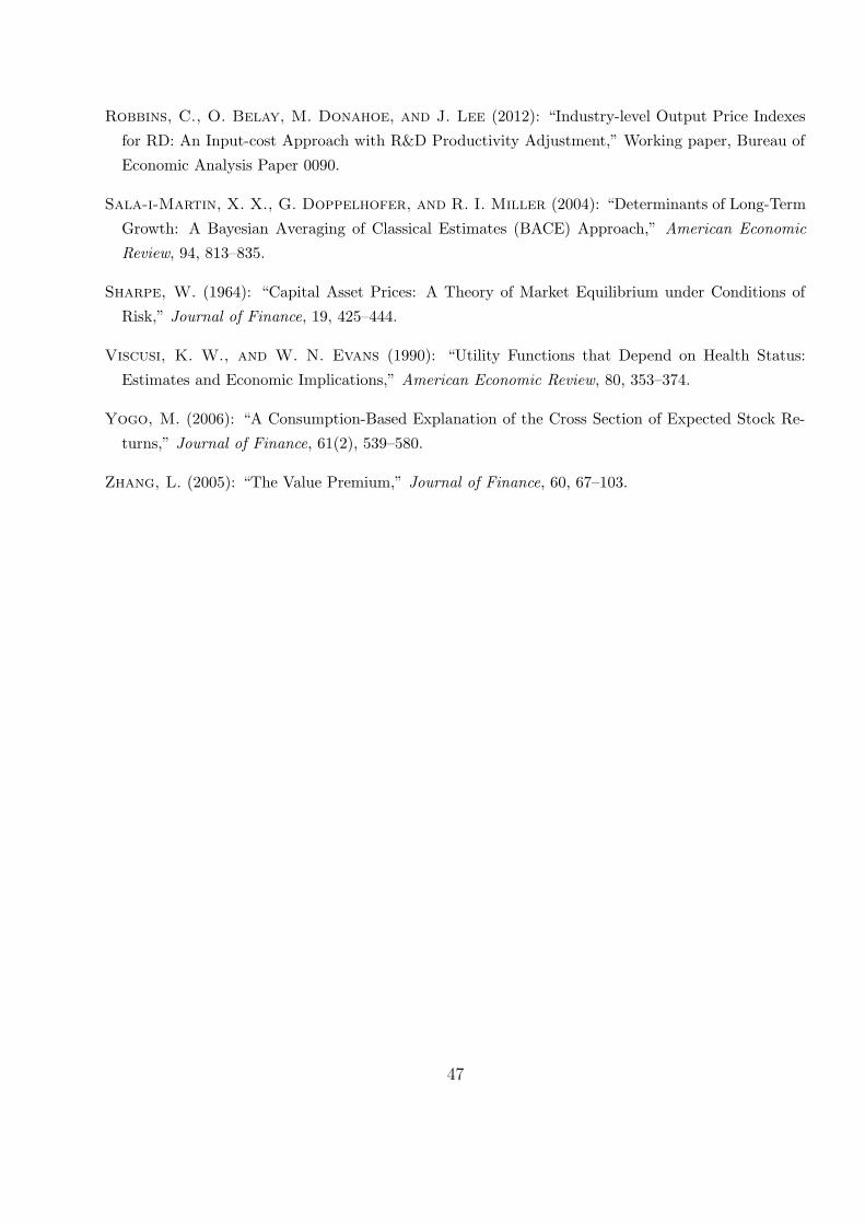
Robbins, C., O. Belay, M. Donahoe, and J. Lee (2012): “Industry-level Output Price Indexes
for RD: An Input-cost Approach with R&D Productivity Adjustment,” Working paper, Bureau of
Economic Analysis Paper 0090.
Sala-i-Martin, X. X., G. Doppelhofer, and R. I. Miller (2004): “Determinants of Long-Term
Growth: A Bayesian Averaging of Classical Estimates (BACE) Approach,” American Economic
Review, 94, 813–835.
Sharpe, W. (1964): “Capital Asset Prices: A Theory of Market Equilibrium under Conditions of
Risk,” Journal of Finance, 19, 425–444.
Viscusi, K. W., and W. N. Evans (1990): “Utility Functions that Depend on Health Status:
Estimates and Economic Implications,” American Economic Review, 80, 353–374.
Yogo, M. (2006): “A Consumption-Based Explanation of the Cross Section of Expected Stock Re-
turns,” Journal of Finance, 61(2), 539–580.
Zhang, L. (2005): “The Value Premium,” Journal of Finance, 60, 67–103.
47
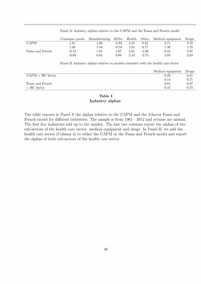
Panel A: Industry alphas relative to the CAPM and the Fama and French model
Consumer goods Manufacturing HiTec Health Other Medical equipment DrugsCAPM 1.81 1.66 -0.83 3.31 0.22 3.71 3.70
1.40 1.54 -0.54 1.61 0.17 1.40 1.78Fama and French -0.13 1.04 1.67 5.01 -2.66 6.44 5.37
-0.09 0.84 0.86 2.44 -2.75 2.05 2.63
Panel B: Industry alphas relative to models extended with the health care factor
Medical equipment DrugsCAPM + HC factor 0.22 0.31
0.14 0.71Fama and French 0.81 0.37+ HC factor 0.47 0.70
Table IIndustry alphas
The table reports in Panel A the alphas relative to the CAPM and the 3-factor Fama andFrench model for different industries. The sample is from 1961 - 2012 and returns are annual.The first five industries add up to the market. The last two columns report the alphas of twosub-sectors of the health care sector: medical equipment and drugs. In Panel B, we add thehealth care sector (Column 4) to either the CAPM or the Fama and French model and reportthe alphas of both sub-sectors of the health care sector.
48

Dictionary to identify government risk
Congress Government regulation(s) Political risk(s)Congressional Government approval PoliticsDebt ceiling Government debt(s) Price constraint(s)Federal Government deficit(s) Price control(s)Federal funds Government intervention(s) Price restriction(s)Fiscal imbalance(s) Law(s) Regulation(s)Government(s) Legal RegulatoryGovernment-approved Legislation Regulatory complianceGovernment-sponsored Legislative Regulatory delay(s)Governmental Legislatory Reimbursement(s)Governmental program(s) Patent law(s) SubsidyGovernment program(s) Political SubsidiesGovernmental regulation(s) Political reform(s)
Table IIDictionary for 10-K filings
The table reports the dictionary that we use to identify how frequently firms highlight riskfactors that are associated with government risk.
49

Panel A: Main dictionary without health care-specific terms
Average word count Average fraction of wordsHealth care sector 138.98 1.51%Non-health care sector 76.58 1.23%
Standard error of difference in means 15.06 0.10%T-statistic 4.14 2.78
Panel B: Dictionary including health care-specific terms
Average word count Average fraction of wordsHealth care sector 180.60 1.89%Non-health care sector 78.86 1.27%
Standard error of difference in means 19.68 0.13%T-statistic 5.17 4.96
Table IIIAverage word count to measure government risk from 10-K filings
Panel A of the table reports the average number of words in a firm’s 10-K filing appears in thedictionary in Table II. The average is taken across the 50 largest firms in the health care sectorand the 50 largest firms in the non-health care sector. The table also reports the standarderror of the difference in means and the corresponding t-statistic. The first column reports theaverage word count, while the second column measures the average fractions of words (that is,word count scaled by the length of the document). Panel B reports the results if we expandthe dictionary to include health care-specific terms that relate to government programs.
50
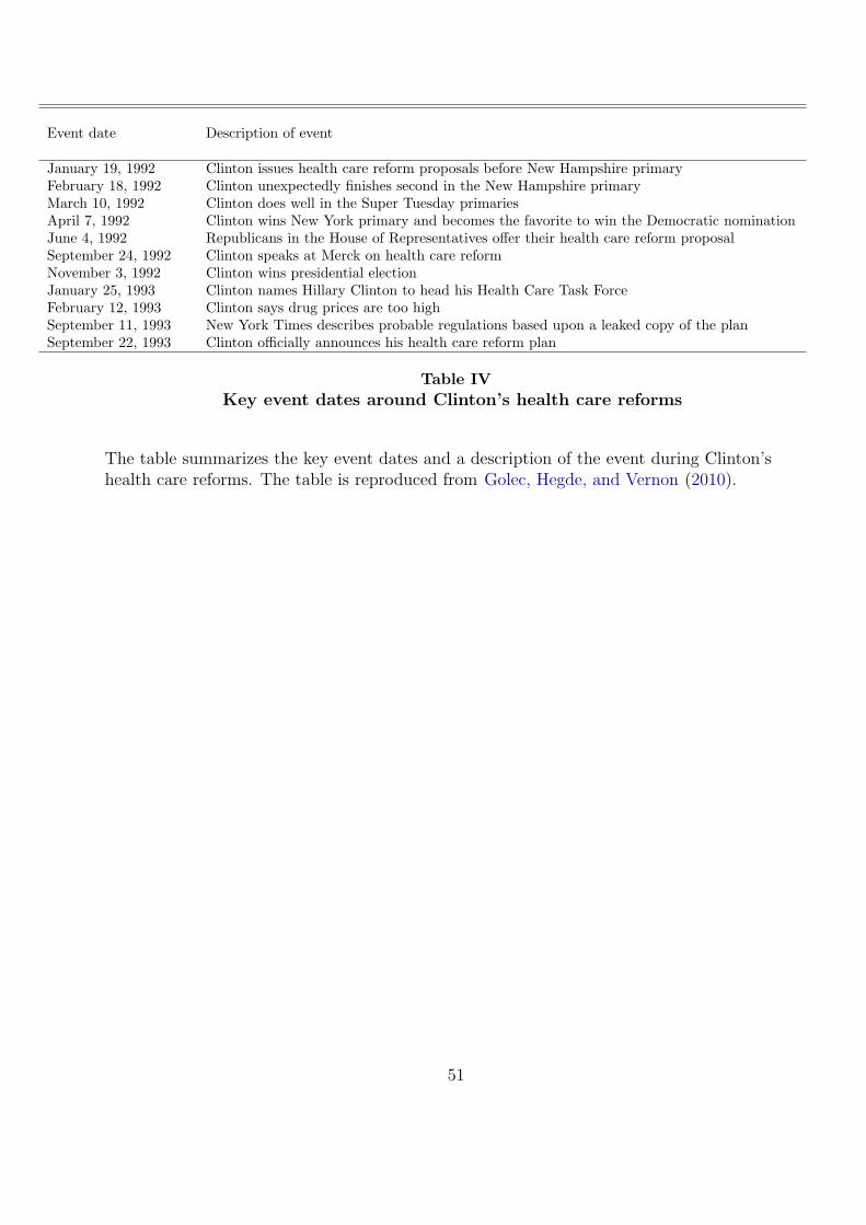
Event date Description of event
January 19, 1992 Clinton issues health care reform proposals before New Hampshire primaryFebruary 18, 1992 Clinton unexpectedly finishes second in the New Hampshire primaryMarch 10, 1992 Clinton does well in the Super Tuesday primariesApril 7, 1992 Clinton wins New York primary and becomes the favorite to win the Democratic nominationJune 4, 1992 Republicans in the House of Representatives offer their health care reform proposalSeptember 24, 1992 Clinton speaks at Merck on health care reformNovember 3, 1992 Clinton wins presidential electionJanuary 25, 1993 Clinton names Hillary Clinton to head his Health Care Task ForceFebruary 12, 1993 Clinton says drug prices are too highSeptember 11, 1993 New York Times describes probable regulations based upon a leaked copy of the planSeptember 22, 1993 Clinton officially announces his health care reform plan
Table IVKey event dates around Clinton’s health care reforms
The table summarizes the key event dates and a description of the event during Clinton’shealth care reforms. The table is reproduced from Golec, Hegde, and Vernon (2010).
51
Intercept -0.21t-statistics -8.28Slope coefficient -7.7%t-statistic -2.66
R-squared 4.0%
Number of firms 327
Average number of years 20.8used to estimate health care betas
Table VCross-sectional regression of cumulative abnormal returns on health care betas
The table reports the results of a cross-sectional regression of the cumulative abnormal returnof a firm during the Clinton health care reform on the beta of a given firm on the health carefactor in (2). The beta is standardized by the cross-sectional standard deviation of the beta.
52

Probability of government intervention
Parameter Description ω = 10% ω = 20%
γ 1.35 1.35φ Markup 3 3ζ Constrained markup 1 1χ R&D subsidy 50% 50%σ Medical care subsidy 50% 50%R Baseline discount rate 1.48 1.48M Price of government risk 0.63 0.63q0 Initial level of medical knowledge 2.80 1.60ν Curvature R&D production function 0.44 0.46h Health endowment 0.45 0.24ξ Weight non-health consumption in U 0.78 0.79
Table VIModel parameters
The table summarizes the calibrated model parameters for two levels of governmentintervention risk (ω).
53

Probability of government intervention: ω = 10%
Benchmark No government risk No government risk premiumHealth share1960 6.1% 6.1% 6.1%1970 7.8% 9.0% 8.7%1980 10.2% 12.8% 12.2%1990 13.2% 17.2% 16.4%2000 16.7% 21.5% 20.6%2010 20.4% 25.3% 24.5%
R&D share1960 0.1% 0.2% 0.2%1970 0.1% 0.5% 0.4%1980 0.2% 0.9% 0.7%1990 0.4% 1.4% 1.1%2000 0.6% 1.9% 1.5%2010 0.8% 2.3% 1.9%
Probability of government intervention: ω = 20%
Benchmark No government risk No government risk premiumHealth share1960 6.1% 6.1% 6.1%1970 7.7% 9.3% 8.7%1980 10.0% 13.7% 12.2%1990 13.0% 18.4% 16.5%2000 16.6% 22.7% 20.7%2010 20.3% 26.2% 24.5%
R&D share1960 0.1% 0.3% 0.2%1970 0.1% 0.7% 0.4%1980 0.2% 1.2% 0.7%1990 0.4% 1.8% 1.1%2000 0.6% 2.3% 1.6%2010 0.8% 2.6% 1.9%
Table VIIHealth and R&D share dynamics for both counterfactuals and different levels of
government risk.
The table illustrates the impact of government risk and the medical innovation premium onhealth care and R&D spending. The first column provides the benchmark results, the secondcolumn removes government risk altogether, while the third column considers thecounterfactual in which there is government risk, but this risk is not priced in equilibrium.
54

1930 1940 1950 1960 1970 1980 1990 2000 20100
0.05
0.1
0.15
0.2
0.25
Share health industryShare devicesShare pharma
Figure 1. Relative market capitalization
The table reports the share of market capitalization of the U.S. stock market that comes fromthe health care industry as well as from drug companies and companies that produce medicaldevices.
55

1990 1995 2000 2005 2010-16
-14
-12
-10
-8
-6
-4
-2
0
Drawdowns health care sectorDrawdowns aggregate market
Discussion Clintonhealth care reform
2000-2002technology crash
2007-2008financial crisis
Figure 2. Drawdown dynamics for the health care sector and the aggregate stock market.
The table reports the drawdown dynamics of the health care sector and the overall stockmarket from 1990 until 2013. Drawdowns are defined in (1).
56
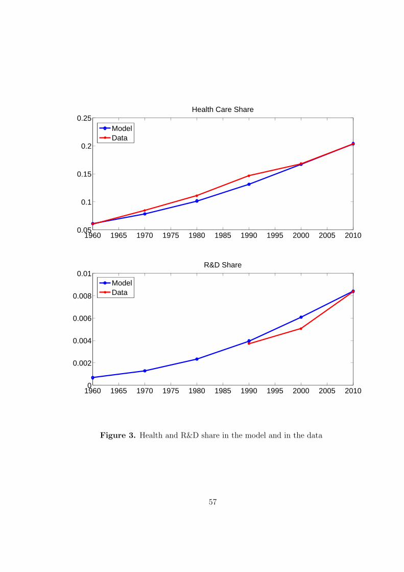
1960 1965 1970 1975 1980 1985 1990 1995 2000 2005 20100.05
0.1
0.15
0.2
0.25Health Care Share
ModelData
1960 1965 1970 1975 1980 1985 1990 1995 2000 2005 20100
0.002
0.004
0.006
0.008
0.01R&D Share
ModelData
Figure 3. Health and R&D share in the model and in the data
57

1960 1965 1970 1975 1980 1985 1990 1995 2000 2005 20100.05
0.1
0.15
0.2
0.25
0.3Health Care Share
1960 1965 1970 1975 1980 1985 1990 1995 2000 2005 20100
0.005
0.01
0.015
0.02
0.025R&D Share
BenchmarkNo government riskNo government risk premium
Figure 4. Counterfactual dynamics of health care and R&D spending
58

1960 1980 2000 2020 2040 2060 2080 2100 2120 2140 21600.05
0.1
0.15
0.2
0.25
0.3
0.35
0.4Health Care Share
1960 1980 2000 2020 2040 2060 2080 2100 2120 2140 21600
0.005
0.01
0.015
0.02R&D Share
Figure 5. Model-implied long-run dynamics of the health and R&D share
59

Online Appendix: Not For Publication
A. Reverse-engineering the preferences of the entrepreneur
Given the numerical solution to the model, it may be instructive to “reverse-engineer”
the preferences, i.e., to find a value function V ({ce,t}t) in terms of the stochastic stream of
entrepreneurial consumptions so that the assumed stochastic discount factors result from the
appropriate first-order conditions. It should be clear that there is considerable freedom in doing
so.
Note that we have assumed (or, for the kinked preference specification, derived) that
Mt+1 = R−1MHt+1
where R is the safe return over the model period of 10 years, and where MHt+1 is the stochastic
component of the discount factor, satisfying 1 = E[MHt+1] and given by
MHt+1 =
M , if Δzt+1 = 1,
M , if Δzt+1 = 0 and zt = 0,
1 , if zt = 1,
Suppose now, that the preferences of the entrepreneur are time separable,
V ({ce,t}t) = E
[∞∑
t=0
βteu(ce,t)
]
The consumption of the entrepreneur ce,t in the absence of government intervention are pro-
portional to profits minus outlays for R&D, as stated in equation (11) of the paper. The con-
sumption of the entrepreneur with government intervention could either be read as zero, or, in
a slight extension of the model, assumed to be some fraction 0 ≤ ξt < 1 of the non-intervention
consumption ce,t at the time of the intervention.
The standard relationships between preferences and stochastic discount factors deliver
R−1M = βeu′(ce,t+1)
u′(ce,t)(40)
R−1M = βeu′(ξtce,t+1)
u′(ce,t)(41)
60

From the numerical calculation done for t = 1, . . . , 6, one finds that entrepreneurial consumption
is growing over time, though not exactly at a constant rate.
The easiest solution to the equations (40) above is to assume that the utility function is
piecewise linear, with a concave kink at some positive level of consumption below ce,1 and with
imposing that ξt takes post-intervention consumption to a level below ce,1: ξt = 0 will be one
possibility that does the trick. With the piecewise linear utility function, one needs to solve for
β per
R−1M = βe (42)
and find the slope below the kink (at c = 0, say) relative to the slope above the kink (at ce,t,
say) perM
M=
u′(0)
u′(ce,t)
Such preferences are a simple version of loss-aversion preferences that have been proposed for
a variety of phenomena, including asset pricing, see Kahneman and Tversky (1979).
If βe does not satisfy (42), but instead is some other value between that value and, say,
β = 1, one can solve the integration problem as follows. For a given value of βe strictly in this
range and with some normalization for u′(ce,1) > 0, calculate recursively
u′(ce,t+1) =M
βeRu′(ce,t)
Note that 0 < u′(ce,t+1) < u′(ce,t). Find a continuous decreasing non-negative function u′(ce)
connecting these points: this is feasible, since ce,t is an increasing sequence. Integrate to find
the utility function u(ce).
While there are many solutions, it may be instructive to see whether one can bound this
exercise, using the CRRA specification. While the CRRA specification will not work exactly,
one can calculate η̄ as the minimal η so that
R−1M ≥ βe
(ce,t+1
ce,t
)−η
, for all t = 1, . . . , 6 (43)
and η as the maximal η, so that
R−1M ≤ βe
(ce,t+1
ce,t
)−η
, for all t = 1, . . . , 6 (44)
Imposing CRRA preferences with these η, one can furthermore ask, what consumption reduction
61
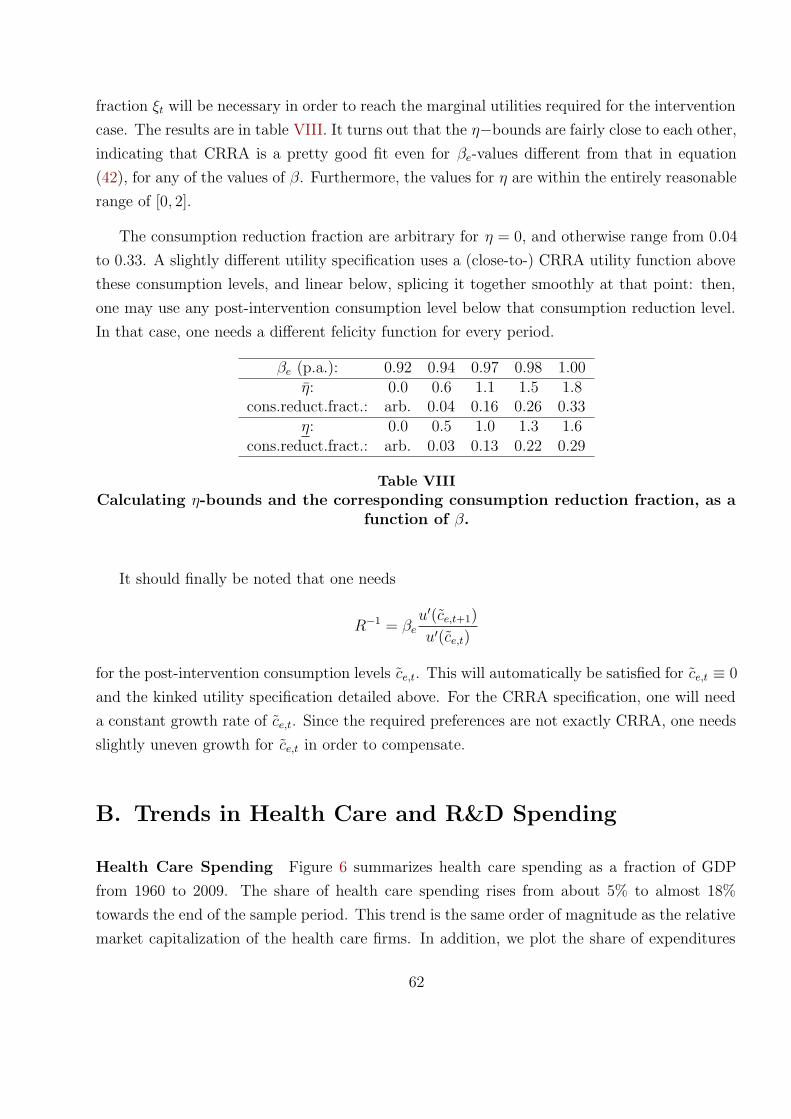
fraction ξt will be necessary in order to reach the marginal utilities required for the intervention
case. The results are in table VIII. It turns out that the η−bounds are fairly close to each other,
indicating that CRRA is a pretty good fit even for βe-values different from that in equation
(42), for any of the values of β. Furthermore, the values for η are within the entirely reasonable
range of [0, 2].
The consumption reduction fraction are arbitrary for η = 0, and otherwise range from 0.04
to 0.33. A slightly different utility specification uses a (close-to-) CRRA utility function above
these consumption levels, and linear below, splicing it together smoothly at that point: then,
one may use any post-intervention consumption level below that consumption reduction level.
In that case, one needs a different felicity function for every period.
βe (p.a.): 0.92 0.94 0.97 0.98 1.00η̄: 0.0 0.6 1.1 1.5 1.8
cons.reduct.fract.: arb. 0.04 0.16 0.26 0.33η: 0.0 0.5 1.0 1.3 1.6
cons.reduct.fract.: arb. 0.03 0.13 0.22 0.29
Table VIIICalculating η-bounds and the corresponding consumption reduction fraction, as a
function of β.
It should finally be noted that one needs
R−1 = βeu′(c̃e,t+1)
u′(c̃e,t)
for the post-intervention consumption levels c̃e,t. This will automatically be satisfied for c̃e,t ≡ 0
and the kinked utility specification detailed above. For the CRRA specification, one will need
a constant growth rate of c̃e,t. Since the required preferences are not exactly CRRA, one needs
slightly uneven growth for c̃e,t in order to compensate.
B. Trends in Health Care and R&D Spending
Health Care Spending Figure 6 summarizes health care spending as a fraction of GDP
from 1960 to 2009. The share of health care spending rises from about 5% to almost 18%
towards the end of the sample period. This trend is the same order of magnitude as the relative
market capitalization of the health care firms. In addition, we plot the share of expenditures
62

on CMS programs, which include Medicare, Medicaid, and CHIP as well as the share coming
from non-CMS programs. This illustrates that all expenditures tend to share a similar trend.
The fact that health expenditures increase as a fraction of GDP is not only a feature of the
US economy, but is more common across OECD countries. Table IX reports the shares in 1971
and 2007 for a large set of countries for which these shares are available. The share of health
expenditures to GDP increased over time for all the countries for which data is available. The
average increase is from 5.6% in 1971 to 9.5% in 2007.
Table IX also reports the fraction of health expenditures that are pharmaceutical expendi-
tures. Our asset pricing facts are largely based on pharmaceutical companies, so we verify that
the trend in overall health expenditures is also present in pharmaceutical expenditures. We find
that this is indeed the case. The share of expenditures that can be attributed to pharmaceutical
expenditures is stable around 14%.
R&D Spending In addition to health spending, medical R&D spending also increased
rapidly over time. Following the methodology in Jones (2011) using data from the OECD,
we plot in Figure 7 the share R&D relative to GDP. The share increased from 0.14% in 1987 to
0.37% in 2006, which compares to 11% to 16% for the share of medical spending to GDP. This
implies that medical R&D spending increased even more rapidly than medical spending itself.
63
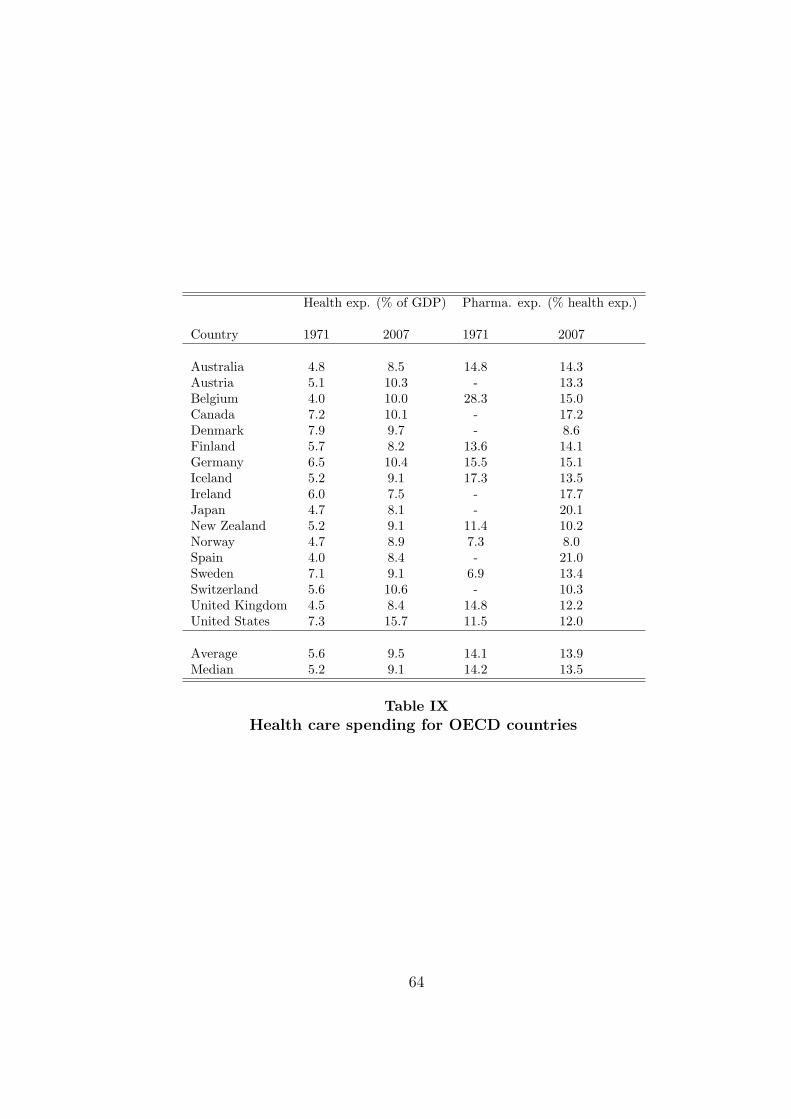
Health exp. (% of GDP) Pharma. exp. (% health exp.)
Country 1971 2007 1971 2007
Australia 4.8 8.5 14.8 14.3Austria 5.1 10.3 - 13.3Belgium 4.0 10.0 28.3 15.0Canada 7.2 10.1 - 17.2Denmark 7.9 9.7 - 8.6Finland 5.7 8.2 13.6 14.1Germany 6.5 10.4 15.5 15.1Iceland 5.2 9.1 17.3 13.5Ireland 6.0 7.5 - 17.7Japan 4.7 8.1 - 20.1New Zealand 5.2 9.1 11.4 10.2Norway 4.7 8.9 7.3 8.0Spain 4.0 8.4 - 21.0Sweden 7.1 9.1 6.9 13.4Switzerland 5.6 10.6 - 10.3United Kingdom 4.5 8.4 14.8 12.2United States 7.3 15.7 11.5 12.0
Average 5.6 9.5 14.1 13.9Median 5.2 9.1 14.2 13.5
Table IXHealth care spending for OECD countries
64

1960 1965 1970 1975 1980 1985 1990 1995 2000 20050
2
4
6
8
10
12
14
16
18
20
Health expenditures/GDPCMS programs/GDPNon-CMS programs/GDP
Figure 6. Medical spending relative to GDP
65
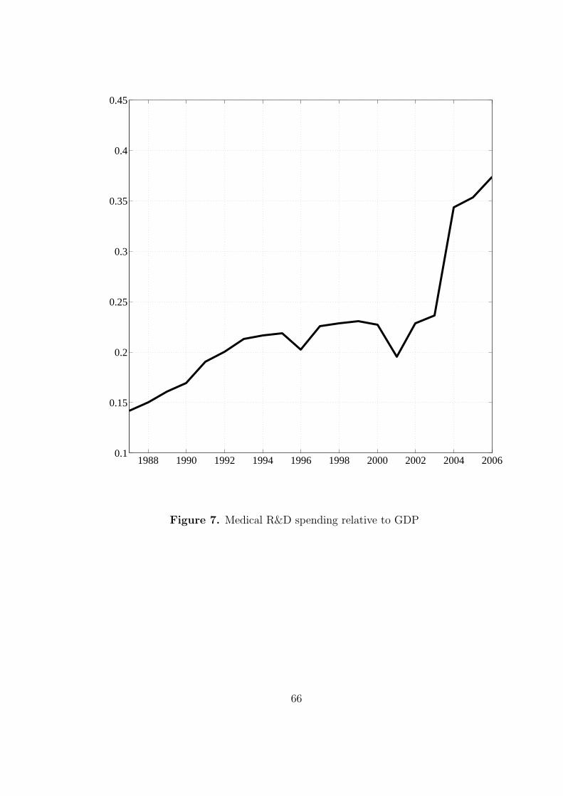
1988 1990 1992 1994 1996 1998 2000 2002 2004 20060.1
0.15
0.2
0.25
0.3
0.35
0.4
0.45
Figure 7. Medical R&D spending relative to GDP
66

C. Robustness of the Medical Innovation Premium
In the main text, we document the medical innovation premium for annual returns for our
main sample from 1961 - 2012 using both the CAPM and the 3-factor Fama and French model.
For robustness, we estimate the model both at a monthly frequency and an annual frequency.
If we estimate the model at a monthly frequency, we multiply the alphas by 12 to annualize them.
We also consider three different sample periods: 1927.1-2013.7, 1946.1-2013.7, and 1961.1-
2013.7. The first sample period is the longest sample available. The second sample focuses on
the post-war period. The third sample coincides with the period for which we have data on
aggregate health care spending. The returns on services start only in the late sixties, and we
therefore exclude them from the table. However, their returns are well explained by standard
models and the alphas are close to zero.
The annual results are in Panel A and the monthly results in Panel B of Table X. The
first number corresponds to the alpha; the second number is the t-statistic using OLS standard
errors. We find that the health care industry tends to produce economically and statistically
significant alphas betwen 3-5% per annum, depending on the benchmark model and the sample
period. If we remove health services and focus on pharmaceutical products and medical equip-
ment, the alphas are even higher at 4-7% per annum. This is because the alphas on medical
services are close to zero.
We also report the alphas on the other industries, which do not have large alphas relative
to the standard models. We typically find that the results are somewhat stronger using the
Fama-French model. We conclude that there is a risk premium for holding health care stocks
that cannot be explained by standard asset pricing factors.
67

Panel A: Annual returns
1927-2012 Consumer goods Manufacturing HiTec Health Other Medical equipment DrugsCAPM 1.25 1.12 0.68 3.98 -0.96 4.33 4.35
1.22 1.49 0.57 2.35 -1.01 2.11 2.48Fama and French 0.78 0.53 2.11 5.56 -2.60 5.80 5.96
0.74 0.74 1.73 3.37 -3.54 2.83 3.42
1946-2012 Consumer goods Manufacturing HiTec Health Other Medical equipment DrugsCAPM 1.19 1.66 -0.29 4.29 -0.86 4.07 4.68
1.07 1.81 -0.21 2.10 -0.77 1.70 2.25Fama and French -0.06 0.92 1.91 5.72 -3.10 6.27 6.06
-0.05 0.96 1.25 2.77 -3.82 2.36 2.87
1961-2012 Consumer goods Manufacturing HiTec Health Other Medical equipment DrugsCAPM 1.81 1.66 -0.83 3.31 0.22 3.71 3.70
1.40 1.54 -0.54 1.61 0.17 1.40 1.78Fama and French -0.13 1.04 1.67 5.01 -2.66 6.44 5.37
-0.09 0.84 0.86 2.44 -2.75 2.05 2.63
Panel B: Monthly returns
1927.1-2013.7 Consumer goods Manufacturing HiTec Health Other Medical equipment DrugsCAPM 1.46 0.74 0.46 3.07 -1.24 3.27 3.47
2.12 1.24 0.52 2.43 -1.50 2.03 2.54Fama and French 1.45 0.26 1.60 3.89 -2.72 3.53 4.34
2.12 0.48 2.06 3.16 -3.91 2.22 3.27
1946.1-2013.7 Consumer goods Manufacturing HiTec Health Other Medical equipment DrugsCAPM 1.25 1.34 -0.59 3.18 -0.92 2.85 3.67
1.61 1.91 -0.58 2.40 -1.12 1.71 2.54Fama and French 0.58 0.25 1.57 4.85 -3.02 3.81 5.50
0.75 0.39 1.75 3.78 -4.13 2.25 3.98
1961.1-2013.7 Consumer goods Manufacturing HiTec Health Other Medical equipment DrugsCAPM 1.76 1.33 -1.01 2.64 -0.10 2.82 3.11
1.92 1.55 -0.84 1.76 -0.10 1.65 1.89Fama and French 0.79 0.17 1.24 4.78 -2.46 4.10 5.54
0.85 0.21 1.14 3.29 -2.82 2.33 3.52
Table XIndustry alphas
68