Working Paper No. 136

Financial Innovations, Money Demand, and the Welfare Cost of Inflation

Aleksander Berentsen, Samuel Huber and Alessandro Marchesiani

January 2014

 

 

 

University of Zurich

Department of Economics

Working Paper Series

ISSN 1664-7041 (print) ISSN 1664-705X (online)

Financial Innovations, Money Demand, and the WelfareCost of Inflation∗

Aleksander BerentsenUniversity of Basel and Federal Reserve Bank of St. Louis

Samuel HuberUniversity of Basel

Alessandro MarchesianiUniversity of Minho

December 16, 2013

Abstract

In the 1990s, the empirical relation between money demand and interest ratesbegan to fall apart. We analyze to what extent improved access to money marketscan explain this break-down. For this purpose, we construct a microfounded mone-tary model with a money market, which provides insurance against liquidity shocksby offering short-term loans and by paying interest on money market deposits. Wecalibrate the model to U.S. data and find that improved access to money marketscan explain the behavior of money demand very well. Furthermore, we show that,by allocating money more effi ciently, better access to money markets decrease thewelfare cost of inflation substantially.

∗For comments on earlier versions of this paper we would like to thank Fabrizio Mattesini, RandallWright, Shouyong Shi, Guillaume Rocheteau, Christian Hellwig, Stephen Williamson and participantsin the JMCB-SNB-UniBern Conference. The views expressed in this article are those of the authorsand not necessarily those of the Federal Reserve Bank of St. Louis, the Federal Reserve System, or theFOMC. Any remaining errors are the authors’responsibility.

1

1 Introduction

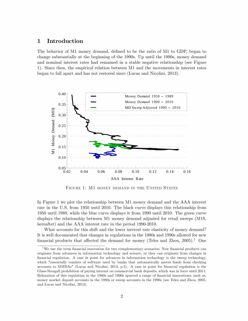
The behavior of M1 money demand, defined to be the ratio of M1 to GDP, began tochange substantially at the beginning of the 1990s. Up until the 1990s, money demandand nominal interest rates had remained in a stable negative relationship (see Figure1). Since then, the empirical relation between M1 and the movements in interest ratesbegan to fall apart and has not restored since (Lucas and Nicolini, 2013).

0.02 0.04 0.06 0.08 0.10 0.12 0.14 0.160.05

0.10

0.15

0.20

0.25

0.30

0.35

0.40

AAA Interest Rate

M1

Mon

eyD

eman

dM

D

MD Sweep Adjusted 1990 2010Money Demand 1990 2010Money Demand 1950 1989

Figure 1: M1 money demand in the United States

In Figure 1 we plot the relationship between M1 money demand and the AAA interestrate in the U.S. from 1950 until 2010. The black curve displays this relationship from1950 until 1989, while the blue curve displays it from 1990 until 2010. The green curvedisplays the relationship between M1 money demand adjusted for retail sweeps (M1S,hereafter) and the AAA interest rate in the period 1990-2010.

What accounts for this shift and the lower interest rate elasticity of money demand?It is well documented that changes in regulations in the 1980s and 1990s allowed for newfinancial products that affected the demand for money (Teles and Zhou, 2005).1 One

1We use the term financial innovation for two complementary scenarios: New financial products canoriginate from advances in information technology and science, or they can originate from changes infinancial regulation. A case in point for advances in information technology is the sweep technology,which "essentially consists of software used by banks that automatically moves funds from checkingaccounts to MMDAs" (Lucas and Nicolini, 2013, p.5). A case in point for financial regulation is theGlass-Steagall prohibition of paying interest on commercial bank deposits, which was in force until 2011.Relaxation of this regulation in the 1980s and 1990s spurred a range of financial innovations; such as,money market deposit accounts in the 1980s or sweep accounts in the 1990s (see Teles and Zhou, 2005,and Lucas and Nicolini, 2013).

2

case in point are retail sweep accounts that were introduced in 1993. VanHoose andHumphrey (2001) report that the introduction of retail sweep accounts reduced requiredbank reserves by more than 70 percent between 1995 and 2000. Thus, the emergenceof sweep accounts can be viewed as a prototypical technical innovation in the financialsector that might explain the downward shift of money demand. However, the greencurve in Figure 1 shows that even when correcting for the impact of retail sweeps, therewas still a substantial change in money demand in the early 1990s.

In order to explain the behavior of money demand, two complementary strategies areavailable. The first strategy is to construct a theoretical model and explore what changesin financial intermediation are needed to replicate the behavior of M1 as observed in thedata, taking the definition of the monetary aggregate M1 as given. The second strategyis to redefine the monetary aggregate in order to better take into account what objects inan economy are used as transaction media of exchange. For example, if M1 is redefinedto include sweep accounts, the changes in the money demand appear to be less dramatic(see Figure 1). A recent paper by Lucas and Nicolini (2013) follows this second strategyby carefully thinking about what objects serve as means of payment and need to beincluded into M1. They then define a new monetary aggregate called NewM1. Thisaggregate adds to the traditional components of M1, demand deposits and currency,the so called MMDAs.2 Finally, they show that there is a stable long-run relationshipbetween the interest rate and NewM1. We will discuss their paper in more detail inSection 7.

Our paper follows the first strategy by taking the definition of money demand asgiven.3 We then construct a monetary model with a financial sector and investigate whatchanges in the financial sector can replicate the observed changes in money demand thatstarted at the beginning of the 1990’s. From a theoretical point of view, innovationsin financial markets can affect money demand via two channels. First, innovations mayallow agents to earn a higher interest rate on their transaction balances. In doing so, suchinnovations make holding the existing money stock more attractive. Second, financialinnovations may allocate the stock of money more effi ciently.

In this paper, we argue that the second channel is responsible for the observed down-ward shift. In particular, we argue that the emergence of money market deposit accountsin the 1980s and the sweep technology in the 1990s is responsible for the observed changesin money demand. In our model, such innovations generate a shift in the theoreticalmoney demand function similar to the one observed in the data. That is to say, theylower money demand and make the money demand curve less elastic.

We derive our results in a microfounded monetary model with a money market.4

In each period, agents face idiosyncratic liquidity shocks which generate an ex-post

2A MMDA (money market deposit account) is a checking account where the holder is only allowedto make a few withdrawals per month.

3Throughout the paper, we work with M1S which is M1 adjusted for retail sweep accounts. Cynamon,Dutkowsky, and Jones (2006) show that the presence of commercial demand deposit sweep programsleads to an underreporting of transactions balances in M1. Detailed information on M1S is available inCynamon, Dutkowsky, and Jones (2007).

4The monetary model is the Lagos and Wright (2005) framework, and the money market is thesame as the one introduced in Berentsen, Camera and Waller (2007, BCW hereafter). Our theoreticalcontribution is that we consider a limited participation version of BCW.

3

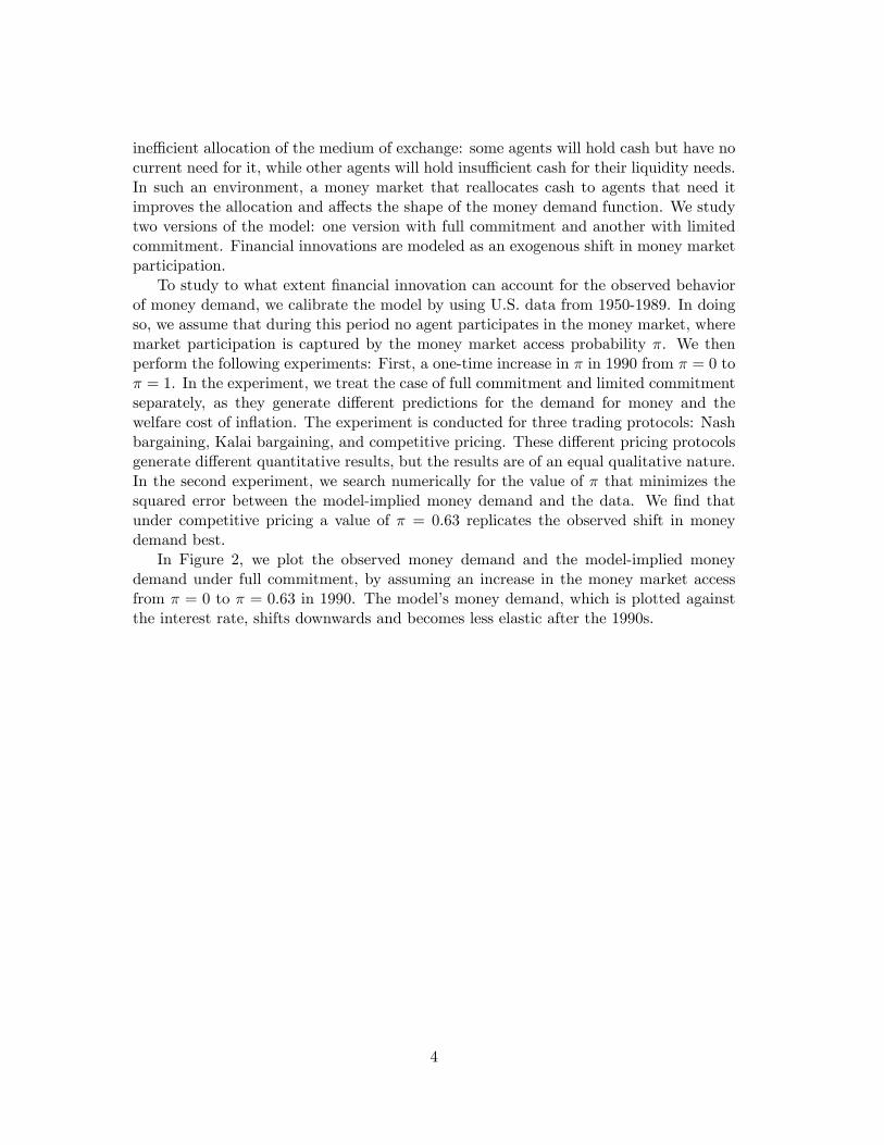
ineffi cient allocation of the medium of exchange: some agents will hold cash but have nocurrent need for it, while other agents will hold insuffi cient cash for their liquidity needs.In such an environment, a money market that reallocates cash to agents that need itimproves the allocation and affects the shape of the money demand function. We studytwo versions of the model: one version with full commitment and another with limitedcommitment. Financial innovations are modeled as an exogenous shift in money marketparticipation.

To study to what extent financial innovation can account for the observed behaviorof money demand, we calibrate the model by using U.S. data from 1950-1989. In doingso, we assume that during this period no agent participates in the money market, wheremarket participation is captured by the money market access probability π. We thenperform the following experiments: First, a one-time increase in π in 1990 from π = 0 toπ = 1. In the experiment, we treat the case of full commitment and limited commitmentseparately, as they generate different predictions for the demand for money and thewelfare cost of inflation. The experiment is conducted for three trading protocols: Nashbargaining, Kalai bargaining, and competitive pricing. These different pricing protocolsgenerate different quantitative results, but the results are of an equal qualitative nature.In the second experiment, we search numerically for the value of π that minimizes thesquared error between the model-implied money demand and the data. We find thatunder competitive pricing a value of π = 0.63 replicates the observed shift in moneydemand best.

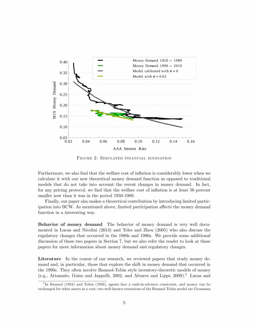
In Figure 2, we plot the observed money demand and the model-implied moneydemand under full commitment, by assuming an increase in the money market accessfrom π = 0 to π = 0.63 in 1990. The model’s money demand, which is plotted againstthe interest rate, shifts downwards and becomes less elastic after the 1990s.

4

0.02 0.04 0.06 0.08 0.10 0.12 0.14 0.160.05

0.10

0.15

0.20

0.25

0.30

0.35

0.40

AAA Interest Rate

M1S

Mon

eyD

eman

d

Model with 0.63Model calibrated with 0Money Demand 1990 2010Money Demand 1950 1989

Figure 2: Simulated financial innovation

Furthermore, we also find that the welfare cost of inflation is considerably lower when wecalculate it with our new theoretical money demand function as opposed to traditionalmodels that do not take into account the recent changes in money demand. In fact,for any pricing protocol, we find that the welfare cost of inflation is at least 50 percentsmaller now than it was in the period 1950-1989.

Finally, our paper also makes a theoretical contribution by introducing limited partic-ipation into BCW. As mentioned above, limited participation affects the money demandfunction in a interesting way.

Behavior of money demand The behavior of money demand is very well docu-mented in Lucas and Nicolini (2013) and Teles and Zhou (2005) who also discuss theregulatory changes that occurred in the 1980s and 1990s. We provide some additionaldiscussion of these two papers in Section 7, but we also refer the reader to look at thesepapers for more information about money demand and regulatory changes.

Literature In the course of our research, we reviewed papers that study money de-mand and, in particular, those that explore the shift in money demand that occurred inthe 1990s. They often involve Baumol-Tobin style inventory-theoretic models of money(e.g., Attanasio, Guiso and Jappelli, 2002, and Alvarez and Lippi, 2009).5 Lucas and

5 In Baumol (1952) and Tobin (1956), agents face a cash-in-advance constraint, and money can beexchanged for other assets at a cost; two well-known extensions of the Baumol-Tobin model are Grossman

5

Nicolini (2013), Ireland (2009), Teles and Zhou (2005) and Reynard (2004) are morerecent attempts to explain the behavior of money demand. Papers that use the searchapproach to monetary economics are Faig and Jerez (2007), and Berentsen, Menzio andWright (2011). We discuss the above-mentioned papers in more detail in Section 7.

Another related branch of the literature are papers that study the welfare cost ofinflation in monetary models with trading frictions; see, e.g., Lagos and Wright (2005),Aruoba, Rocheteau and Waller (2007), Craig and Rocheteau (2007), and Chiu andMolico (2010), among many others.6 Some other related papers study issues such ascredit card use (Telyukova and Wright, 2008, and Rojas-Breu, 2013) and its effect onmoney demand (Telyukova, 2013), and the impact of aggregate and idiosyncratic shockson money demand over the business cycle (Telyukova and Visschers, 2012). The mainfocus of our work is to investigate the quantitative effects of financial innovation onsteady state money demand and velocity.

2 Environment

There is a [0, 1] continuum of infinitely-lived agents.7 Time is discrete, and in each periodthere are three markets that open sequentially: a frictionlessmoney market, where agentscan borrow and deposit money; a goods market, where production and consumption of aspecialized good take place; and a centralized market, where credit contracts are settledand a general good is produced and consumed. All goods are nonstorable, which meansthat they cannot be carried from one market to the next.

At the beginning of each period, agents receive two i.i.d. shocks: a preference shockand an entry shock. The preference shock determines whether an agent can consume orproduce the specialized good in the goods market: with probability n, he can producebut not consume, while with probability 1 − n, he can consume but not produce. Werefer to producers as sellers and to consumers as buyers. The entry shock determineswhether an agent has access to a frictionless money market: with probability π he hasaccess, while with probability 1− π he does not. Agents who have access to the moneymarket are called active, while agents who have no access are called passive.

In the goods market, buyers and sellers meet at random and bargain over the terms oftrade. The matching process is described according to a reduced-form matching function,M (n, 1− n), whereM is the number of trade matches in a period. We assume that thematching function has constant returns to scale, and is continuous and increasing with

and Weiss (1983) and Rotemberg (1984). Examples of inventory-theoretic models of money demand withmarket segmentation are Alvarez, Lucas and Weber (2001), Alvarez, Atkeson and Kehoe (2002), andAlvarez, Atkeson and Edmond (2009). Silber (1983) provides a survey of the financial innovations thatoccurred in the period 1950-1980. He argues that both financial innovations and technological changesrespond to economic incentives, and that both are welfare-improving. In particular, he documents thatfinancial innovation improves protection against risk and reduces transaction costs.

6The literature on the welfare cost of inflation has been initiated by Bailey (1956) and Friedman(1969). Subsequent works include, but are not limited to, Fischer (1981), Lucas (1981), and Cooley andHansen (1989, 1991). Most of these papers are cash-in-advance or money-in-the-utility-function models.

7The basic environment is similar to BCW which builds on Lagos and Wright (2005). The Lagosand Wright framework is useful, because it allows us to introduce heterogeneity while still keeping thedistribution of money holdings analytically tractable.

6

respect to each of its arguments. Let δ (n) =M (n, 1− n) (1− n)−1 be the probabilitythat a buyer meets a seller, and δs (n) = δ (n) (1− n)n−1 be the probability that a sellermeets a buyer. In what follows, we suppress the argument n and refer to δ (n) and δs (n)as δ and δs, respectively.

In the goods market, a buyer receives utility u(q) from consuming q units of thespecialized good, where u(q) satisfies u′(q) > 0, u′′(q) < 0, u′(0) = +∞, and u′(∞) = 0.A seller incurs a utility cost c (q) = q from producing q units. Furthermore, agentsare anonymous and agents’actions are not publicly observed. These assumptions meanthat an agent’s promise to pay in the future is not credible, and sellers require imme-diate compensation for their production. Therefore, a means of exchange is needed fortransactions.8

The general good can be produced and consumed by all agents and is traded in africtionless, centralized market. Agents receive utility U(x) from consuming x units,where U ′ (x) ,−U ′′ (x) > 0, U ′ (0) = ∞, and U ′ (∞) = 0. They produce the generalgood with a linear technology, such that one unit of x is produced with one unit oflabor, which generates one unit of disutility h. This assumption eliminates the wealtheffect, which makes the end-of-period distribution of money degenerate (see Lagos andWright, 2005). Agents discount between, but not within, periods. Let β ∈ (0, 1) be thediscount factor between two consecutive periods.

There exists an object, called money, that serves as a medium of exchange. It isperfectly storable and divisible, and has no intrinsic value. The supply of money evolvesaccording to the low of motion Mt+1 = γMt, where γ ≥ β denotes the gross growthrate of money and Mt the stock of money in t. In the centralized market, each agentreceives a lump-sum transfer Tt = Mt+1 −Mt = (γ − 1)Mt. To economize on notation,next-period variables are indexed by +1, and previous-period variables are indexed by−1.

The money market is modeled similar to the one in BCW. In the money marketperfectly competitive financial intermediaries take deposits and make loans, which allowsagents to adjust their money balances before entering the goods market. In particular,an agent with high liquidity needs can borrow money, while an agent with low liquidityneeds can deposit money and earn interest. All credit contracts are one-period contractsand are redeemed in the centralized market. Financial intermediaries operate a record-keeping technology that keeps track of all agents’past credit transactions at zero cost.Perfect competition among financial intermediaries in the money market implies thatthe deposit rate, id, is equal to the loan rate, i`. Throughout the paper, the commonnominal interest rate is denoted by i.

BCW provide a detailed description of the environment that allows for the coexistenceof fiat money and credit. We refer the reader to their paper for further details. In thispaper, we generalize BCW by assuming that only a fraction, π ≤ 1, of agents have accessto the money market in each period. Like in BCW, we study two cases: full commitmentand limited commitment. Under full commitment, there is no default. Under limitedcommitment, debt repayment is voluntary. The only punishment for those who default is

8The role of anonymity in these models has been studied, for example, by Araujo (2004) and Alipran-tis, Camera and Puzzello (2007).

7

permanent exclusion from the money market. For this punishment, we derive conditionssuch that debt repayment is voluntary.

3 Full commitment

In what follows, we present the agents’decision problems within a representative period,t. We proceed backwards, moving from the last to the first market. All proofs arerelegated to the Appendix.

The centralized market. In the centralized market, agents can consume and producethe centralized market good x. Furthermore, they receive money for their deposits plusinterest payments. Additionally, they have to pay back their loans plus interest. Anagent entering the centralized market with m units of money, ` units of loans, and dunits of deposits has the value function V3(m, `, d). He solves the following decisionproblem

V3(m, `, d) = maxx,h,m+1

U(x)− h+ βV1(m+1), (1)

subject to the budget constraint

x+ φm+1 = h+ φm+ φT + φ (1 + i) d− φ (1 + i) `, (2)

where h denotes hours worked and φ denotes the price of money in terms of the generalgood. As in Lagos and Wright (2005), we show in the Appendix that the choice of m+1

is independent of m. As a result, each agent exits the centralized market with the sameamount of money, and, thus, the distribution of money holdings is degenerate at thebeginning of a period.

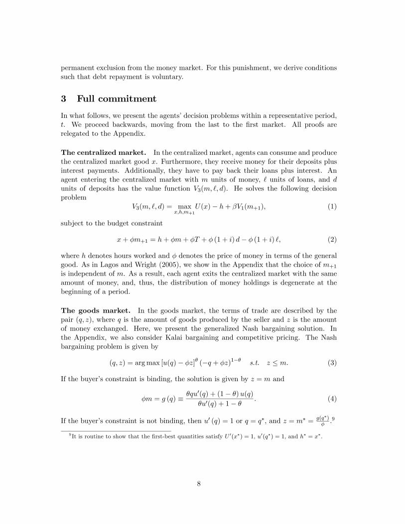
The goods market. In the goods market, the terms of trade are described by thepair (q, z), where q is the amount of goods produced by the seller and z is the amountof money exchanged. Here, we present the generalized Nash bargaining solution. Inthe Appendix, we also consider Kalai bargaining and competitive pricing. The Nashbargaining problem is given by

(q, z) = arg max [u(q)− φz]θ (−q + φz)1−θ s.t. z ≤ m. (3)

If the buyer’s constraint is binding, the solution is given by z = m and

φm = g (q) ≡ θqu′(q) + (1− θ)u(q)

θu′(q) + 1− θ . (4)

If the buyer’s constraint is not binding, then u′ (q) = 1 or q = q∗, and z = m∗ = g(q∗)φ .9

9 It is routine to show that the first-best quantities satisfy U ′(x∗) = 1, u′(q∗) = 1, and h∗ = x∗.

8

The money market. At the beginning of each period, an agent learns his type; thatis, whether he is a buyer or seller and his participation status in the money market(active or passive). Let V b

1 (m) and V s1 (m) be the value functions of an active buyer

and an active seller, respectively, in the money market. Accordingly, the value functionof an agent at the beginning of each period is

V1 (m) = π[(1− n)V b

1 (m) + nV s1 (m)

]+ (1− π)

[(1− n)V b

2 (m) + nV s2 (m)

]. (5)

An agent in the money market is an active buyer with probability π (1− n), an activeseller with probability πn, a passive buyer with probability (1− π) (1− n), and a passiveseller with probability (1− π)n. Passive agents in the money market just wait for thegoods market to open, so their utility function in the money market is equal to theirutility function in the goods market.

An active buyer’s problem in the money market is

V b1 (m) = max

`V b

2 (m+ `, `) , (6)

and an active seller’s problem in the money market is

V s1 (m) = max

dV s

2 (m− d, d) s.t. m− d ≥ 0. (7)

The constraint in (7) means that a seller cannot deposit more money than what he has.Let λs be the Lagrange multiplier on this constraint. As we will see below, the natureof the equilibrium will depend on whether this constraint is binding or not.

In an economy with full commitment, there are two types of equilibria: an equilibriumwhere active sellers do not deposit all their money (i.e., λs = 0), and another equilibriumwhere active sellers deposit all their money (i.e., λs > 0). We refer to these equilibria asthe type-A and type-B equilibrium, respectively.

3.1 Type-A equilibrium

In the type-A equilibrium, active sellers do not deposit all their money. For this to hold,sellers must be indifferent between depositing their money and not depositing it. Thiscan be only the case if and only if i = 0.

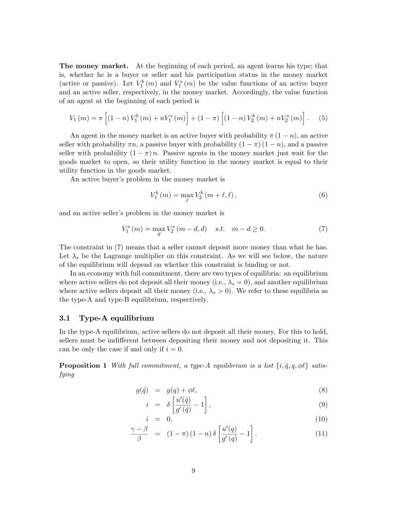
Proposition 1 With full commitment, a type-A equilibrium is a list {i, q, q, φ`} satis-fying

g(q) = g(q) + φ`, (8)

i = δ

[u′(q)

g′ (q)− 1

], (9)

i = 0, (10)γ − ββ

= (1− π) (1− n) δ

[u′(q)

g′ (q)− 1

]. (11)

9

According to Proposition 1, with full commitment in a type-A equilibrium, the fol-lowing holds. From (8), the real amount of money an active buyer spends in the goodsmarket, g(q), is equal to the real amount of money spent as a passive buyer, g(q), plusthe real loan an active buyer gets from the bank, φ`. Equation (8) is derived fromthe active buyer’s budget constraint and immediately shows that in this equilibriumq > q. An active buyer’s consumption satisfies equation (9), which is derived from thefirst-order condition for the choice of loans, `. Equation (10) is derived from the seller’sdeposit choice in the money market. In the proof of Proposition 1, we show that thefirst-order condition is φi = λs, and since λs = 0, we have i = 0; together with (9), thisimplies u′(q) = g′ (q). From (11), a passive buyer consumes an ineffi ciently low quantityof goods in the goods market unless γ = β. This last equation is derived from the choiceof money holdings in the centralized market.

As in BCW, to obtain the first-best allocation q = q = q∗, the central bank needs toset γ = β. Note further that as π → 1, q → 0. The reason for this is the following: ifthe chance that agents have no access is small, then the value of money is small as well.However, note that as π → 1, the economy does not remain in the type-A equilibrium.Rather, it switches to the type-B equilibrium as explained below.

3.2 Type-B equilibrium

In the type-B equilibrium, active sellers deposit all their money at the bank, and so thedeposit constraint is binding; i.e., λs > 0. For this to hold, the nominal interest ratemust be strictly positive. In this case, we have:

Proposition 2 With full commitment, a type-B equilibrium is a list {i, q, q, φ`} satisfy-ing

g(q) = g(q) + φ`, (12)

i = δ

[u′(q)

g′ (q)− 1

], (13)

g (q) = (1− n) g (q) , (14)γ − ββ

= πδ

[u′(q)

g′ (q)− 1

]+ (1− π) (1− n) δ

[u′(q)

g′ (q)− 1

]. (15)

Equations (12), (13), and (15) in Proposition 2, have the same meaning as theircounterparts in Proposition 1. In contrast, equation (10) must be replaced by the marketclearing condition in the money market (14).

Let γ be the value of γ such that equations (11) and (15) hold simultaneously; i.e.,u′(q) = g′ (q). Then, the following holds: (i) for any β < γ ≤ γ, then λs = 0; (ii) for anyγ > γ, then λs > 0.

3.3 Discussion

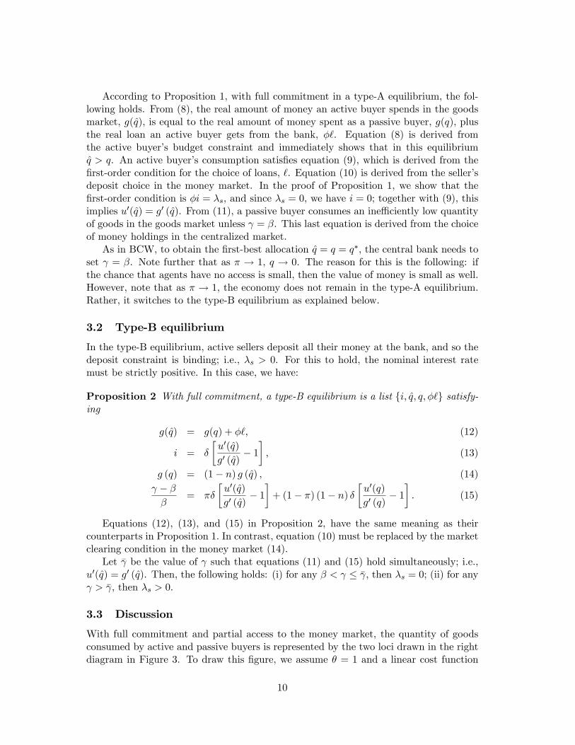
With full commitment and partial access to the money market, the quantity of goodsconsumed by active and passive buyers is represented by the two loci drawn in the rightdiagram in Figure 3. To draw this figure, we assume θ = 1 and a linear cost function

10

c(q) = q.10 The dotted (solid) line denotes the consumed quantity by an active (passive)buyer as a function of γ.

Figure 3: Consumed quantities under full commitment

In the type-A equilibrium, an active buyer’s consumption is independent of γ and equalto q∗, while a passive buyer’s consumption is decreasing in γ and smaller than q∗ unlessβ = γ. In the type-B equilibrium, both the active and passive buyers’ consumptionis decreasing in γ. The dotted vertical line that separates the two equilibria intersectsthe horizontal axis at γ = γ. How does γ change in the rate of participation π? Ournumerical examples show that γ is decreasing in π with γ → β as π → 1. Hence, with fullcommitment and full participation, the type-A equilibrium exists under the Friedmanrule only, while the type-B equilibrium exists for any γ > β. The diagram on the leftin Figure 3 shows the consumed quantities for the full participation case (i.e., π = 1).In this case, all agents are active, and the first best consumption is achieved at theFriedman rule.

4 Limited commitment

In an economy with limited commitment, an active buyer decides whether to repay hisdebt or not. We assume that the only punishment available for an agent who doesnot repay his loan is permanent exclusion from the money market.11 As in BCW, thisassumption generates an endogenous borrowing constraint which we will derive below.

A buyer who defaults on his loan faces a trade-off. On one hand, by not repaying, hebenefits from not having to work in order to repay the loan and the interest on the loanin the current period. On the other hand, he will suffer from future losses, in terms ofless consumption, since he will be denied access to credit forever. If the current benefitis smaller than the expected value of all future losses, a deviation is not profitable andthe buyer repays his loan.10The shapes of the curves in Figure 3 do not change qualitatively for θ < 1.11By the one-step deviation principle, we could exclude an agent by one period only and allow him to

return to the financial sector provided he repays his past debt including accrued interest.

11

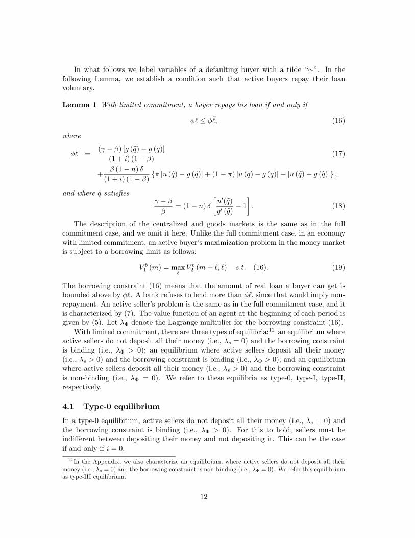
In what follows we label variables of a defaulting buyer with a tilde “∼”. In thefollowing Lemma, we establish a condition such that active buyers repay their loanvoluntary.

Lemma 1 With limited commitment, a buyer repays his loan if and only if

φ` ≤ φ¯, (16)

where

φ¯ =(γ − β) [g (q)− g (q)]

(1 + i) (1− β)(17)

+β (1− n) δ

(1 + i) (1− β){π [u (q)− g (q)] + (1− π) [u (q)− g (q)]− [u (q)− g (q)]} ,

and where q satisfiesγ − ββ

= (1− n) δ

[u′(q)

g′ (q)− 1

]. (18)

The description of the centralized and goods markets is the same as in the fullcommitment case, and we omit it here. Unlike the full commitment case, in an economywith limited commitment, an active buyer’s maximization problem in the money marketis subject to a borrowing limit as follows:

V b1 (m) = max

`V b

2 (m+ `, `) s.t. (16). (19)

The borrowing constraint (16) means that the amount of real loan a buyer can get isbounded above by φ¯. A bank refuses to lend more than φ¯, since that would imply non-repayment. An active seller’s problem is the same as in the full commitment case, and itis characterized by (7). The value function of an agent at the beginning of each period isgiven by (5). Let λΦ denote the Lagrange multiplier for the borrowing constraint (16).

With limited commitment, there are three types of equilibria:12 an equilibrium whereactive sellers do not deposit all their money (i.e., λs = 0) and the borrowing constraintis binding (i.e., λΦ > 0); an equilibrium where active sellers deposit all their money(i.e., λs > 0) and the borrowing constraint is binding (i.e., λΦ > 0); and an equilibriumwhere active sellers deposit all their money (i.e., λs > 0) and the borrowing constraintis non-binding (i.e., λΦ = 0). We refer to these equilibria as type-0, type-I, type-II,respectively.

4.1 Type-0 equilibrium

In a type-0 equilibrium, active sellers do not deposit all their money (i.e., λs = 0) andthe borrowing constraint is binding (i.e., λΦ > 0). For this to hold, sellers must beindifferent between depositing their money and not depositing it. This can be the caseif and only if i = 0.12 In the Appendix, we also characterize an equilibrium, where active sellers do not deposit all their

money (i.e., λs = 0) and the borrowing constraint is non-binding (i.e., λΦ = 0). We refer this equilibriumas type-III equilibrium.

12

Proposition 3 With limited commitment, a type-0 equilibrium is a list {i, q, q, q, φ`, φ¯}satisfying (17), (18), and

g(q) = g(q) + φ`, (20)

φ` = φ¯, (21)

i = 0, (22)γ − ββ

= (1− n) δ

{π

[u′(q)

g′ (q)− 1

]+ (1− π)

[u′(q)

g′ (q)− 1

]}, (23)

The meaning of equations (20), (22), and (23) is identical to that of their counterpartsin Propositions 1 and 2. Unlike the full commitment case, an active buyer is borrowing-constrained in the type-0 equilibrium. This immediately implies that the marginal valueof borrowing is higher than its marginal cost. Hence, neither equation (9) nor (13) holdhere. These equations are replaced by (21). Moreover, with limited commitment we alsoneed to characterize the endogenous borrowing constraint and the consumption quantityof a defaulter as in equations (17) and (18), respectively.

The system of equations in Proposition 3 admits at least one solution which is thestraightforward solution q = q = q. To see this, assume q = q. Then, from (20), it holdsthat φ` = 0. Furthermore, (23) collapses to (18), implying q = q. This means that thetwo terms on the right side of (17) are both zero, and, thus, φ¯ = 0. Therefore, weconclude that the above-mentioned quantities are equilibrium quantities.

However, we cannot show analytically that no other equilibrium exists. In fact, to thecontrary, we identified, numerically, equilibria where q∗ > q > q > q and φ` = φ¯> 0.

4.2 Type-I equilibrium

In a type-I equilibrium, active sellers deposit all their money (i.e., λs > 0), and theborrowing constraint is binding (i.e., λΦ > 0). In a type-I equilibrium, we have

Proposition 4 With limited commitment, a type-I equilibrium is a list{i, q, q, q, φ`, φ¯

}satisfying (17), (18), and

g(q) = g(q) + φ`, (24)

φ` = φ¯, (25)

g (q) = (1− n) g (q) , (26)γ − ββ

= π

{(1− n) δ

[u′(q)

g′ (q)− 1

]+ ni

}+ (1− π) (1− n) δ

[u′(q)

g′ (q)− 1

]. (27)

All the equations in Proposition 4 have the same meaning as their counterparts inProposition 3, except that (22) is now replaced by (26) which comes from the moneymarket clearing condition. Equation (26) does not appear in Proposition 3, since sellersdo not deposit all their money in a type-0 equilibrium, while they do it in a type-Iequilibrium.

13

4.3 Type-II equilibrium

In a type-II equilibrium, active sellers deposit all their money (i.e., λs > 0), and thebuyer’s borrowing constraint is non-binding (i.e., λΦ = 0).

Proposition 5 With limited commitment, a type-II equilibrium is a list{i, q, q, q, φ`, φ¯

}satisfying (17), (18), and

g(q) = g(q) + φ`, (28)

i = δ

[u′(q)

g′ (q)− 1

], (29)

g (q) = (1− n) g (q) , (30)γ − ββ

= πδ

[u′(q)

g′ (q)− 1

]+ (1− π) (1− n) δ

[u′(q)

g′ (q)− 1

]. (31)

All the equations in Proposition 5 have the same meaning as the respective equationsin Proposition 4, except that (25) is now replaced by (29). The meaning of equation (29)is the following. In a type-II equilibrium, active buyers are not borrowing-constrained,which means that they borrow up to the point where the marginal cost of borrowing anadditional unit of money (left side) is equal to the marginal benefit (right side). Note that

δ[u′(q)g′(q) − 1

]> i in type-0 and type-I equilibria, since buyers are borrowing-constrained,

and so they cannot borrow the optimal amount of money.Finally, notice that (28)-(31) are identical to the respective equations in Proposition

2. This is not surprising, since active buyers are not borrowing-constrained in a type-II equilibrium. Hence, in this region, the perfect and limited commitment economiesimplement the same allocation.

4.4 Sequence of equilibria

Let γ1 be the value of γ that separates type-0 and type-I equilibria, and γ2 be the valueof γ that separates type-I and type-II equilibria. This can then be rendered in a sequenceof equilibria which are summarized in Table 1.

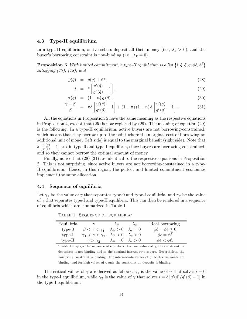
Table 1: Sequence of equilibriaa

Equilibria γ λΦ λs Real borrowingtype-0 β < γ < γ1 λΦ > 0 λs = 0 φ` = φ¯≥ 0type-I γ1 < γ < γ2 λΦ > 0 λs > 0 φ` = φ¯

type-II γ > γ2 λΦ = 0 λs > 0 φ` < φ¯.aTable 1 displays the sequence of equilibria. For low values of γ, the constraint on

depositors is not binding and so the nominal interest rate is zero. Nevertheless, the

borrowing constraint is binding. For intermediate values of γ, both constraints are

binding, and for high values of γ only the constraint on deposits is binding.

The critical values of γ are derived as follows: γ1 is the value of γ that solves i = 0in the type-I equilibrium, while γ2 is the value of γ that solves i = δ [u′(q)/g′ (q)− 1] inthe type-I equilibrium.

14

The region β < γ ≤ γ1 can be further divided into two subregions. In the firstsubregion, there is an equilibrium with φ¯> 0 and q∗ > q > q > q if 0 < π < 1. In thesecond subregion, there is a unique equilibrium which satisfies φ¯ = 0 and q = q = q.To distinguish these regions, we numerically find a third threshold, γ0, such that ifγ0 < γ ≤ γ1, the economy is in the first subregion, and if β < γ < γ0, it is in the secondsubregion.

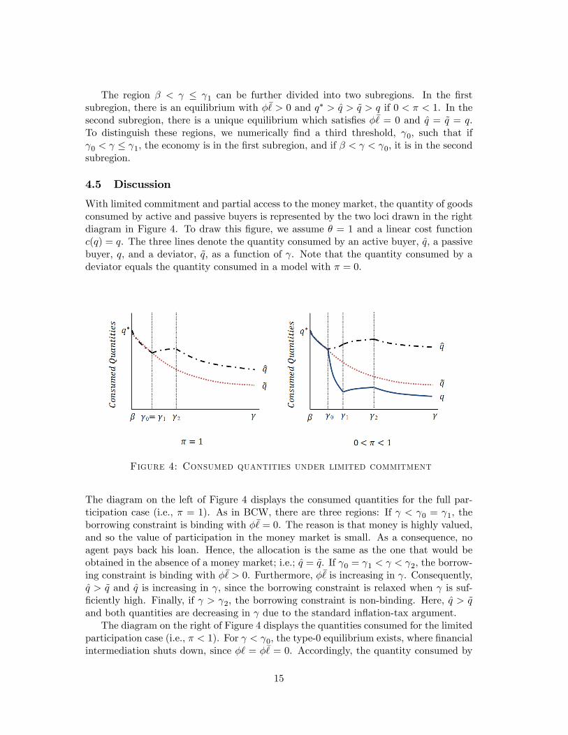
4.5 Discussion

With limited commitment and partial access to the money market, the quantity of goodsconsumed by active and passive buyers is represented by the two loci drawn in the rightdiagram in Figure 4. To draw this figure, we assume θ = 1 and a linear cost functionc(q) = q. The three lines denote the quantity consumed by an active buyer, q, a passivebuyer, q, and a deviator, q, as a function of γ. Note that the quantity consumed by adeviator equals the quantity consumed in a model with π = 0.

Figure 4: Consumed quantities under limited commitment

The diagram on the left of Figure 4 displays the consumed quantities for the full par-ticipation case (i.e., π = 1). As in BCW, there are three regions: If γ < γ0 = γ1, theborrowing constraint is binding with φ¯= 0. The reason is that money is highly valued,and so the value of participation in the money market is small. As a consequence, noagent pays back his loan. Hence, the allocation is the same as the one that would beobtained in the absence of a money market; i.e.; q = q. If γ0 = γ1 < γ < γ2, the borrow-ing constraint is binding with φ¯> 0. Furthermore, φ¯ is increasing in γ. Consequently,q > q and q is increasing in γ, since the borrowing constraint is relaxed when γ is suf-ficiently high. Finally, if γ > γ2, the borrowing constraint is non-binding. Here, q > qand both quantities are decreasing in γ due to the standard inflation-tax argument.

The diagram on the right of Figure 4 displays the quantities consumed for the limitedparticipation case (i.e., π < 1). For γ < γ0, the type-0 equilibrium exists, where financialintermediation shuts down, since φ` = φ¯ = 0. Accordingly, the quantity consumed by

15

active and passive agents equals the quantity consumed by a deviator and is decreasingin γ. For γ0 < γ < γ1, the type-0 equilibrium exists, where borrowing is constrained withφ` = φ¯> 0, and the consumption of active agents is increasing and the consumption ofpassive agents is decreasing in γ. For γ1 < γ < γ2, the type-I equilibrium exists, whereborrowing is constrained and the consumption of active and passive agents is increasingin γ. For γ > γ2, the type-II equilibrium exists, where borrowing is unconstrained andthe consumption of active and passive agents is decreasing in γ.

The separation of these regions is indicated by the vertical dotted lines labeled γ0,γ1 and γ2, respectively. Our numerical examples show that the critical values, γ1 andγ2, are decreasing in the rate of participation, π, with γ1 → 1 as π → 1. This is becausea lower value of π reduces the chance of having access to the money market and thusincreases the incentive to default.

We now show how the velocity of money behaves under limited commitment. Themodel’s velocity of money is derived as follows: The real output in the goods market isYGM = (1− n) δ [πφm+ (1− π)φm], where φm = g(q) and φM−1 = φm = g(q), andthe real output in the centralized market is YCM = A for U (x) = A log(x). Accordingly,the total real output of the economy is Y = YGM +YCM , and the model-implied velocityof money is

v =Y

φM−1=A+ (1− n) δ [πg(q) + (1− π) g(q)]

g(q).

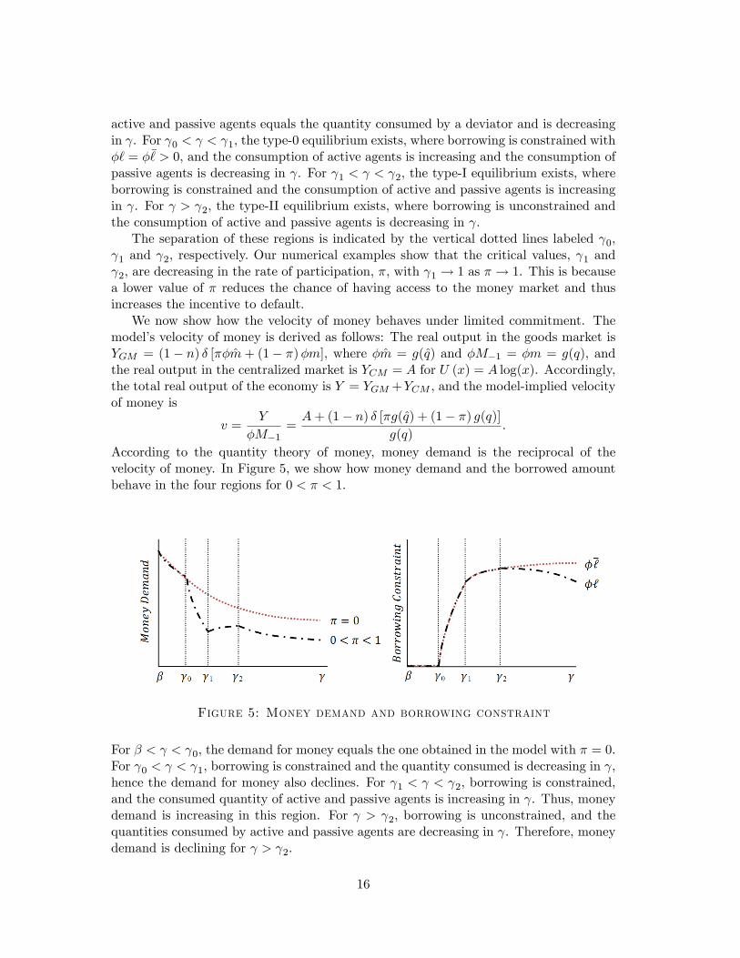
According to the quantity theory of money, money demand is the reciprocal of thevelocity of money. In Figure 5, we show how money demand and the borrowed amountbehave in the four regions for 0 < π < 1.

Figure 5: Money demand and borrowing constraint

For β < γ < γ0, the demand for money equals the one obtained in the model with π = 0.For γ0 < γ < γ1, borrowing is constrained and the quantity consumed is decreasing in γ,hence the demand for money also declines. For γ1 < γ < γ2, borrowing is constrained,and the consumed quantity of active and passive agents is increasing in γ. Thus, moneydemand is increasing in this region. For γ > γ2, borrowing is unconstrained, and thequantities consumed by active and passive agents are decreasing in γ. Therefore, moneydemand is declining for γ > γ2.

16

5 Quantitative analysis

We choose a model period of one year. The functions u(q), U(x), and c(q) have theforms u (q) = q1−α/(1 − α), U (x) = A log(x), and c(q) = q, respectively. Regardingthe matching function, we follow Kiyotaki and Wright (1993) and choose M(B,S) =BS/(B + S), where B = 1 − n is the measure of buyers, and S = n is the measure ofsellers. Therefore, the matching probability of a buyer in the goods market is equal toδ =M(1− n, n) ∗ (1− n)−1 = n.

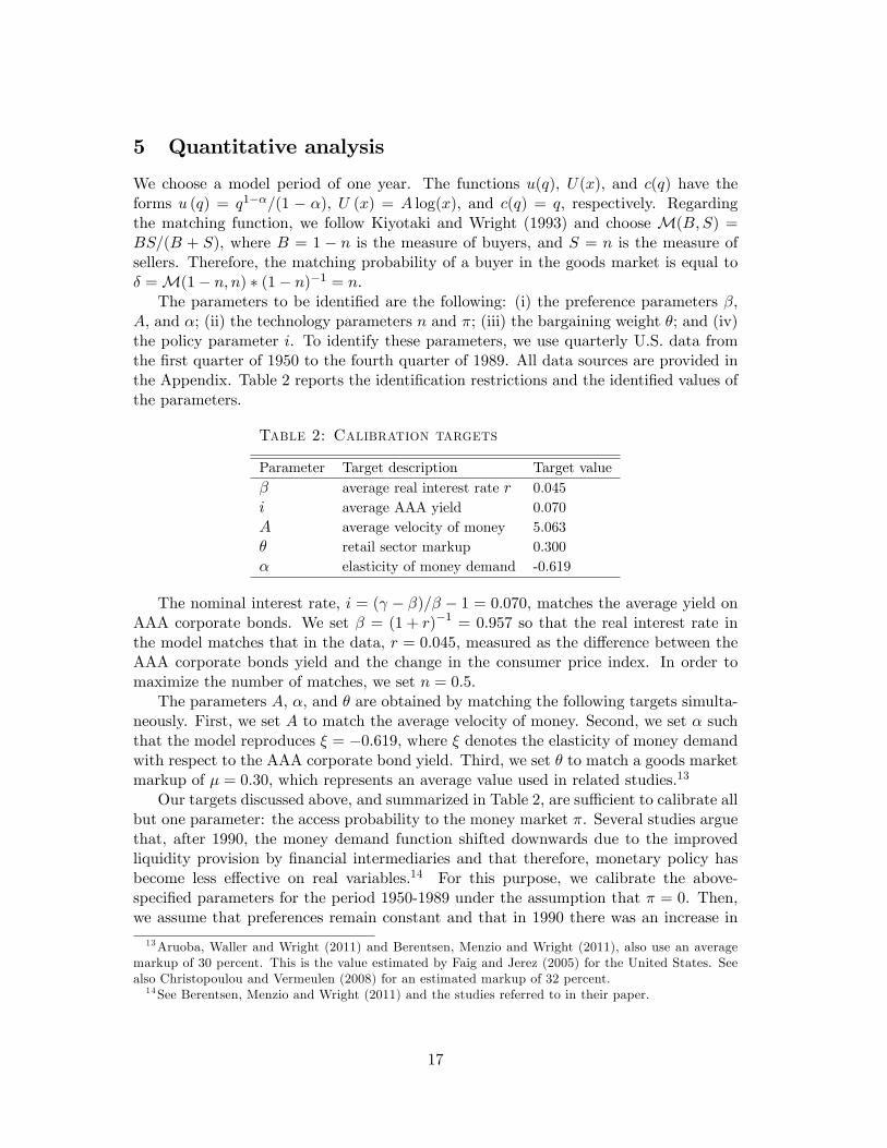
The parameters to be identified are the following: (i) the preference parameters β,A, and α; (ii) the technology parameters n and π; (iii) the bargaining weight θ; and (iv)the policy parameter i. To identify these parameters, we use quarterly U.S. data fromthe first quarter of 1950 to the fourth quarter of 1989. All data sources are provided inthe Appendix. Table 2 reports the identification restrictions and the identified values ofthe parameters.

Table 2: Calibration targets

Parameter Target description Target valueβ average real interest rate r 0.045i average AAA yield 0.070A average velocity of money 5.063θ retail sector markup 0.300α elasticity of money demand -0.619

The nominal interest rate, i = (γ − β)/β − 1 = 0.070, matches the average yield onAAA corporate bonds. We set β = (1 + r)−1 = 0.957 so that the real interest rate inthe model matches that in the data, r = 0.045, measured as the difference between theAAA corporate bonds yield and the change in the consumer price index. In order tomaximize the number of matches, we set n = 0.5.

The parameters A, α, and θ are obtained by matching the following targets simulta-neously. First, we set A to match the average velocity of money. Second, we set α suchthat the model reproduces ξ = −0.619, where ξ denotes the elasticity of money demandwith respect to the AAA corporate bond yield. Third, we set θ to match a goods marketmarkup of µ = 0.30, which represents an average value used in related studies.13

Our targets discussed above, and summarized in Table 2, are suffi cient to calibrate allbut one parameter: the access probability to the money market π. Several studies arguethat, after 1990, the money demand function shifted downwards due to the improvedliquidity provision by financial intermediaries and that therefore, monetary policy hasbecome less effective on real variables.14 For this purpose, we calibrate the above-specified parameters for the period 1950-1989 under the assumption that π = 0. Then,we assume that preferences remain constant and that in 1990 there was an increase in

13Aruoba, Waller and Wright (2011) and Berentsen, Menzio and Wright (2011), also use an averagemarkup of 30 percent. This is the value estimated by Faig and Jerez (2005) for the United States. Seealso Christopoulou and Vermeulen (2008) for an estimated markup of 32 percent.14See Berentsen, Menzio and Wright (2011) and the studies referred to in their paper.

17

π. This allows us to estimate to what extent financial intermediation can account forthe observed shift in money demand.

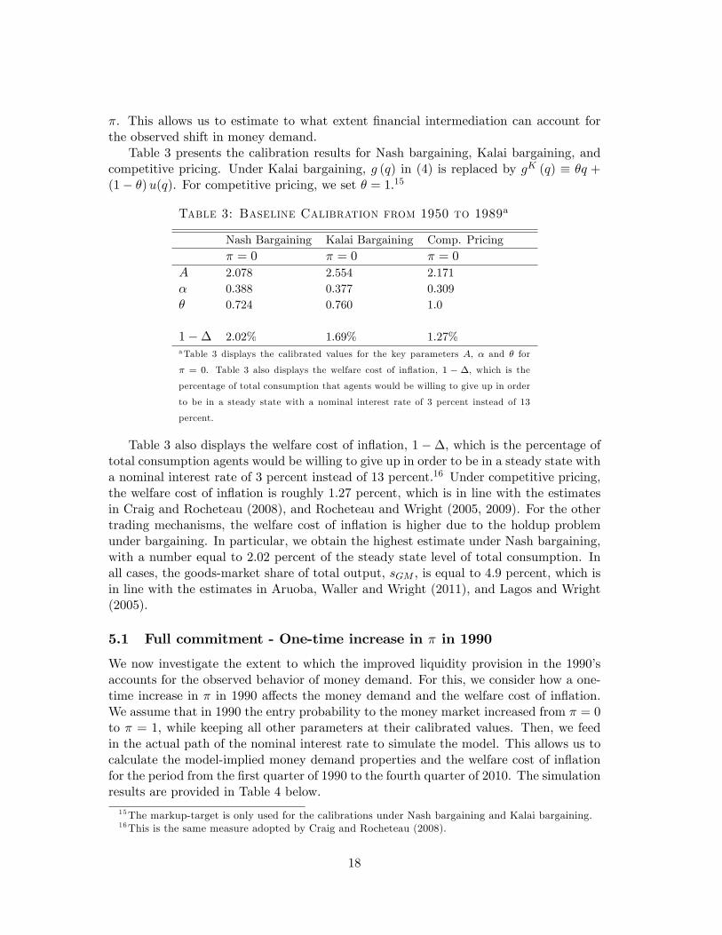
Table 3 presents the calibration results for Nash bargaining, Kalai bargaining, andcompetitive pricing. Under Kalai bargaining, g (q) in (4) is replaced by gK (q) ≡ θq +(1− θ)u(q). For competitive pricing, we set θ = 1.15

Table 3: Baseline Calibration from 1950 to 1989a

Nash Bargaining Kalai Bargaining Comp. Pricingπ = 0 π = 0 π = 0

A 2.078 2.554 2.171α 0.388 0.377 0.309θ 0.724 0.760 1.0

1−∆ 2.02% 1.69% 1.27%aTable 3 displays the calibrated values for the key parameters A, α and θ for

π = 0. Table 3 also displays the welfare cost of inflation, 1 − ∆, which is the

percentage of total consumption that agents would be willing to give up in order

to be in a steady state with a nominal interest rate of 3 percent instead of 13

percent.

Table 3 also displays the welfare cost of inflation, 1−∆, which is the percentage oftotal consumption agents would be willing to give up in order to be in a steady state witha nominal interest rate of 3 percent instead of 13 percent.16 Under competitive pricing,the welfare cost of inflation is roughly 1.27 percent, which is in line with the estimatesin Craig and Rocheteau (2008), and Rocheteau and Wright (2005, 2009). For the othertrading mechanisms, the welfare cost of inflation is higher due to the holdup problemunder bargaining. In particular, we obtain the highest estimate under Nash bargaining,with a number equal to 2.02 percent of the steady state level of total consumption. Inall cases, the goods-market share of total output, sGM , is equal to 4.9 percent, which isin line with the estimates in Aruoba, Waller and Wright (2011), and Lagos and Wright(2005).

5.1 Full commitment - One-time increase in π in 1990

We now investigate the extent to which the improved liquidity provision in the 1990’saccounts for the observed behavior of money demand. For this, we consider how a one-time increase in π in 1990 affects the money demand and the welfare cost of inflation.We assume that in 1990 the entry probability to the money market increased from π = 0to π = 1, while keeping all other parameters at their calibrated values. Then, we feedin the actual path of the nominal interest rate to simulate the model. This allows us tocalculate the model-implied money demand properties and the welfare cost of inflationfor the period from the first quarter of 1990 to the fourth quarter of 2010. The simulationresults are provided in Table 4 below.

15The markup-target is only used for the calibrations under Nash bargaining and Kalai bargaining.16This is the same measure adopted by Craig and Rocheteau (2008).

18

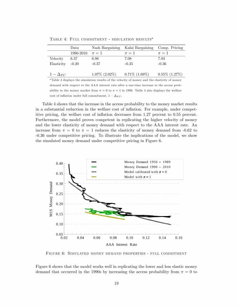
Table 4: Full commitment - simulation resultsa

Data Nash Bargaining Kalai Bargaining Comp. Pricing1990-2010 π = 1 π = 1 π = 1

Velocity 6.37 6.98 7.08 7.03Elasticity -0.20 -0.37 -0.35 -0.36

1−∆FC 1.07% (2.02%) 0.71% (1.69%) 0.55% (1.27%)aTable 4 displays the simulation results of the velocity of money and the elasticity of money

demand with respect to the AAA interest rate after a one-time increase in the access prob-

ability to the money market from π = 0 to π = 1 in 1990. Table 4 also displays the welfare

cost of inflation under full commitment, 1−∆FC .

Table 4 shows that the increase in the access probability to the money market resultsin a substantial reduction in the welfare cost of inflation. For example, under compet-itive pricing, the welfare cost of inflation decreases from 1.27 percent to 0.55 percent.Furthermore, the model proves competent in replicating the higher velocity of moneyand the lower elasticity of money demand with respect to the AAA interest rate. Anincrease from π = 0 to π = 1 reduces the elasticity of money demand from -0.62 to-0.36 under competitive pricing. To illustrate the implications of the model, we showthe simulated money demand under competitive pricing in Figure 6.

0.02 0.04 0.06 0.08 0.10 0.12 0.14 0.160.05

0.10

0.15

0.20

0.25

0.30

0.35

0.40

AAA Interest Rate

M1S

Mon

eyD

eman

d

Model with 1Model calibrated with 0Money Demand 1990 2010Money Demand 1950 1989

Figure 6: Simulated money demand properties - full commitment

Figure 6 shows that the model works well in replicating the lower and less elastic moneydemand that occurred in the 1990s by increasing the access probability from π = 0 to

19

π = 1.

5.2 Limited commitment - One-time increase in π in 1990

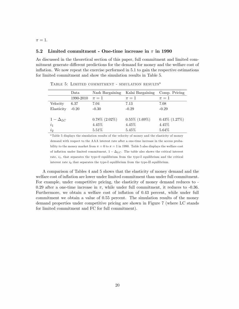
As discussed in the theoretical section of this paper, full commitment and limited com-mitment generate different predictions for the demand for money and the welfare cost ofinflation. We now repeat the exercise performed in 5.1 to gain the respective estimationsfor limited commitment and show the simulation results in Table 5.

Table 5: Limited commitment - simulation resultsa

Data Nash Bargaining Kalai Bargaining Comp. Pricing1990-2010 π = 1 π = 1 π = 1

Velocity 6.37 7.04 7.13 7.08Elasticity -0.20 -0.30 -0.29 -0.29

1−∆LC 0.78% (2.02%) 0.55% (1.69%) 0.43% (1.27%)i1 4.45% 4.45% 4.45%i2 5.51% 5.45% 5.64%aTable 5 displays the simulation results of the velocity of money and the elasticity of money

demand with respect to the AAA interest rate after a one-time increase in the access proba-

bility to the money market from π = 0 to π = 1 in 1990. Table 5 also displays the welfare cost

of inflation under limited commitment, 1 −∆LC . The table also shows the critical interest

rate, i1, that separates the type-0 equilibrium from the type-I equilibrium and the critical

interest rate i2 that separates the type-I equilibrium from the type-II equilibrium.

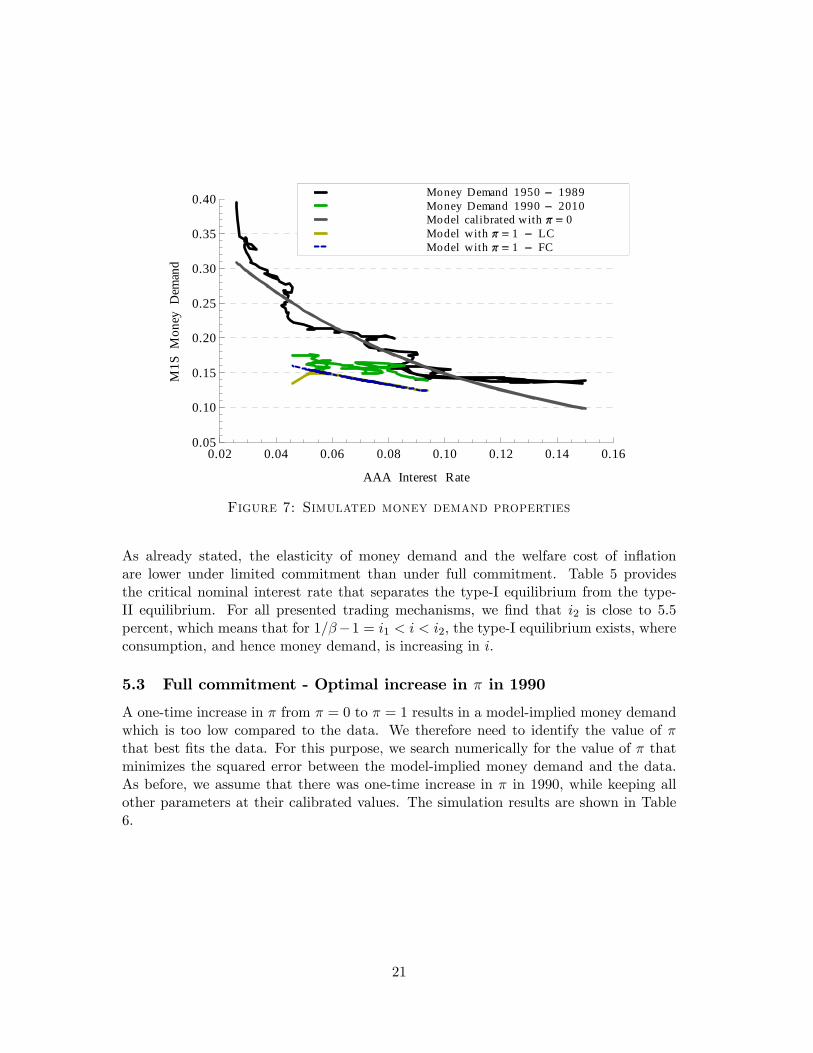
A comparison of Tables 4 and 5 shows that the elasticity of money demand and thewelfare cost of inflation are lower under limited commitment than under full commitment.For example, under competitive pricing, the elasticity of money demand reduces to -0.29 after a one-time increase in π, while under full commitment, it reduces to -0.36.Furthermore, we obtain a welfare cost of inflation of 0.43 percent, while under fullcommitment we obtain a value of 0.55 percent. The simulation results of the moneydemand properties under competitive pricing are shown in Figure 7 (where LC standsfor limited commitment and FC for full commitment).

20

0.02 0.04 0.06 0.08 0.10 0.12 0.14 0.160.05

0.10

0.15

0.20

0.25

0.30

0.35

0.40

AAA Interest Rate

M1S

Mon

eyD

eman

d

Model with 1 FCModel with 1 LCModel calibrated with 0Money Demand 1990 2010Money Demand 1950 1989

Figure 7: Simulated money demand properties

As already stated, the elasticity of money demand and the welfare cost of inflationare lower under limited commitment than under full commitment. Table 5 providesthe critical nominal interest rate that separates the type-I equilibrium from the type-II equilibrium. For all presented trading mechanisms, we find that i2 is close to 5.5percent, which means that for 1/β−1 = i1 < i < i2, the type-I equilibrium exists, whereconsumption, and hence money demand, is increasing in i.

5.3 Full commitment - Optimal increase in π in 1990

A one-time increase in π from π = 0 to π = 1 results in a model-implied money demandwhich is too low compared to the data. We therefore need to identify the value of πthat best fits the data. For this purpose, we search numerically for the value of π thatminimizes the squared error between the model-implied money demand and the data.As before, we assume that there was one-time increase in π in 1990, while keeping allother parameters at their calibrated values. The simulation results are shown in Table6.

21

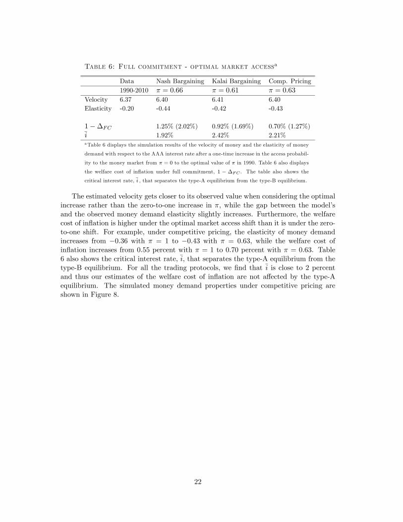
Table 6: Full commitment - optimal market accessa

Data Nash Bargaining Kalai Bargaining Comp. Pricing1990-2010 π = 0.66 π = 0.61 π = 0.63

Velocity 6.37 6.40 6.41 6.40Elasticity -0.20 -0.44 -0.42 -0.43

1−∆FC 1.25% (2.02%) 0.92% (1.69%) 0.70% (1.27%)i 1.92% 2.42% 2.21%aTable 6 displays the simulation results of the velocity of money and the elasticity of money

demand with respect to the AAA interest rate after a one-time increase in the access probabil-

ity to the money market from π = 0 to the optimal value of π in 1990. Table 6 also displays

the welfare cost of inflation under full commitment, 1 − ∆FC . The table also shows the

critical interest rate, i , that separates the type-A equilibrium from the type-B equilibrium.

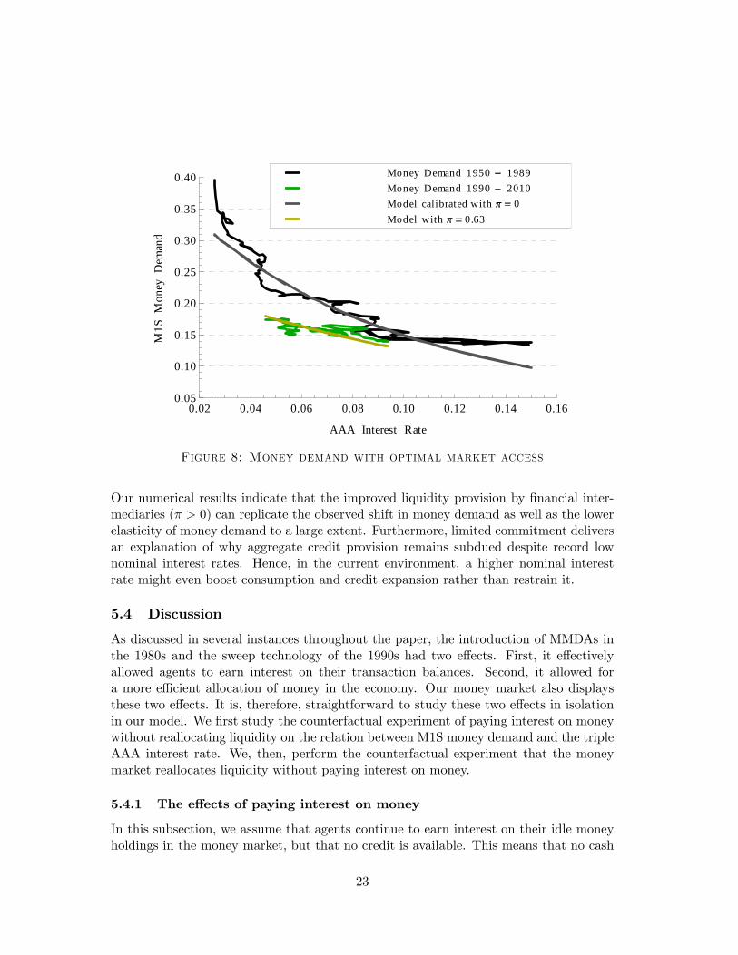
The estimated velocity gets closer to its observed value when considering the optimalincrease rather than the zero-to-one increase in π, while the gap between the model’sand the observed money demand elasticity slightly increases. Furthermore, the welfarecost of inflation is higher under the optimal market access shift than it is under the zero-to-one shift. For example, under competitive pricing, the elasticity of money demandincreases from −0.36 with π = 1 to −0.43 with π = 0.63, while the welfare cost ofinflation increases from 0.55 percent with π = 1 to 0.70 percent with π = 0.63. Table6 also shows the critical interest rate, i, that separates the type-A equilibrium from thetype-B equilibrium. For all the trading protocols, we find that i is close to 2 percentand thus our estimates of the welfare cost of inflation are not affected by the type-Aequilibrium. The simulated money demand properties under competitive pricing areshown in Figure 8.

22

0.02 0.04 0.06 0.08 0.10 0.12 0.14 0.160.05

0.10

0.15

0.20

0.25

0.30

0.35

0.40

AAA Interest Rate

M1S

Mon

eyD

eman

d

Model with 0.63Model calibrated with 0Money Demand 1990 2010Money Demand 1950 1989

Figure 8: Money demand with optimal market access

Our numerical results indicate that the improved liquidity provision by financial inter-mediaries (π > 0) can replicate the observed shift in money demand as well as the lowerelasticity of money demand to a large extent. Furthermore, limited commitment deliversan explanation of why aggregate credit provision remains subdued despite record lownominal interest rates. Hence, in the current environment, a higher nominal interestrate might even boost consumption and credit expansion rather than restrain it.

5.4 Discussion

As discussed in several instances throughout the paper, the introduction of MMDAs inthe 1980s and the sweep technology of the 1990s had two effects. First, it effectivelyallowed agents to earn interest on their transaction balances. Second, it allowed fora more effi cient allocation of money in the economy. Our money market also displaysthese two effects. It is, therefore, straightforward to study these two effects in isolationin our model. We first study the counterfactual experiment of paying interest on moneywithout reallocating liquidity on the relation between M1S money demand and the tripleAAA interest rate. We, then, perform the counterfactual experiment that the moneymarket reallocates liquidity without paying interest on money.

5.4.1 The effects of paying interest on money

In this subsection, we assume that agents continue to earn interest on their idle moneyholdings in the money market, but that no credit is available. This means that no cash

23

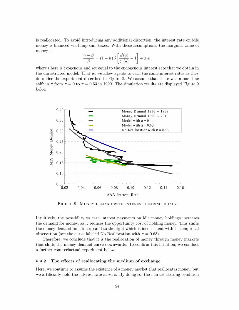
is reallocated. To avoid introducing any additional distortion, the interest rate on idlemoney is financed via lump-sum taxes. With these assumptions, the marginal value ofmoney is

γ − ββ

= (1− n) δ

[u′(q)

g′ (q)− 1

]+ πni,

where i here is exogenous and set equal to the endogenous interest rate that we obtain inthe unrestricted model. That is, we allow agents to earn the same interest rates as theydo under the experiment described in Figure 8. We assume that there was a one-timeshift in π from π = 0 to π = 0.63 in 1990. The simulation results are displayed Figure 9below.

0.02 0.04 0.06 0.08 0.10 0.12 0.14 0.160.05

0.10

0.15

0.20

0.25

0.30

0.35

0.40

AAA Interest Rate

M1S

Mon

eyD

eman

d No Reallocation with 0.63Model with 0.63Model with 0Money Demand 1990 2010Money Demand 1950 1989

Figure 9: Money demand with interest-bearing money

Intuitively, the possibility to earn interest payments on idle money holdings increasesthe demand for money, as it reduces the opportunity cost of holding money. This shiftsthe money demand function up and to the right which is inconsistent with the empiricalobservation (see the curve labeled No Reallocation with π = 0.63).

Therefore, we conclude that it is the reallocation of money through money marketsthat shifts the money demand curve downwards. To confirm this intuition, we conducta further counterfactual experiment below.

5.4.2 The effects of reallocating the medium of exchange

Here, we continue to assume the existence of a money market that reallocates money, butwe artificially hold the interest rate at zero. By doing so, the market clearing condition

24

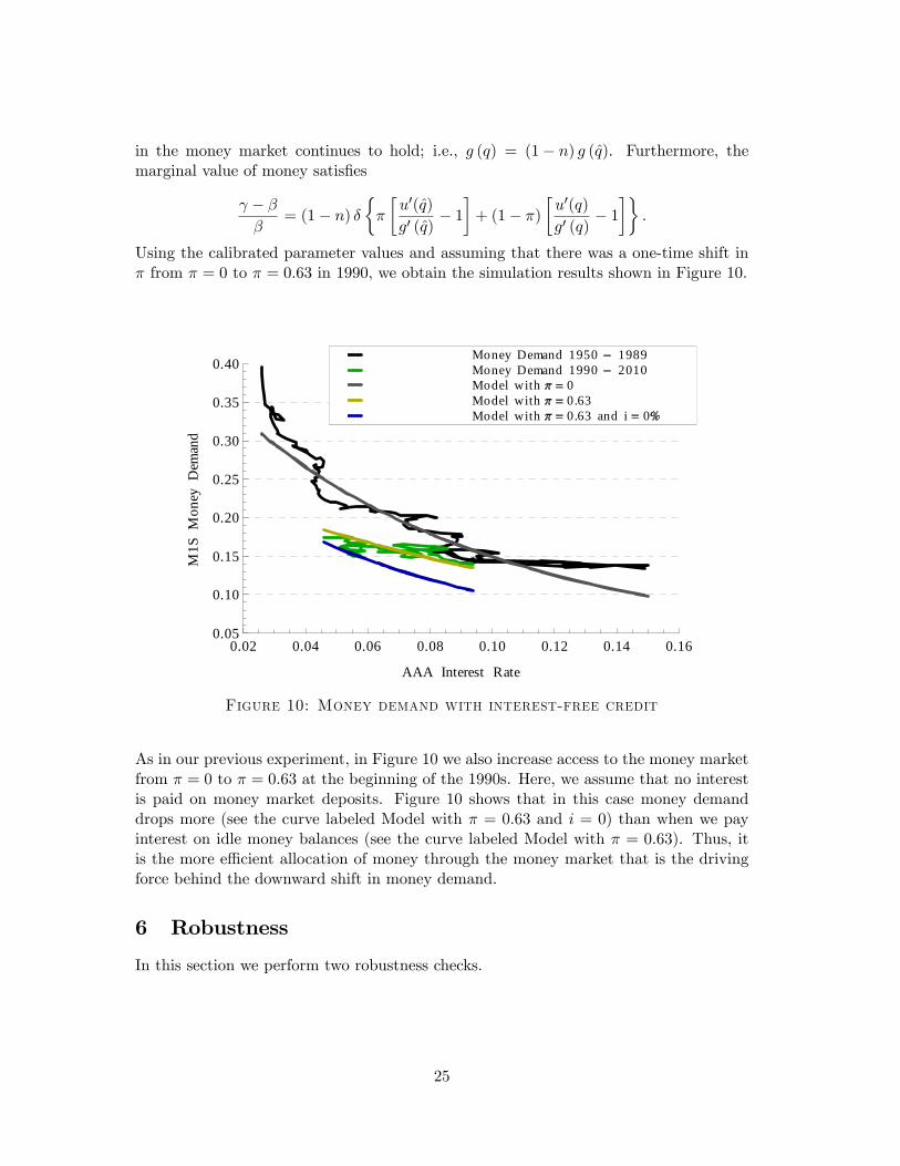
in the money market continues to hold; i.e., g (q) = (1− n) g (q). Furthermore, themarginal value of money satisfies

γ − ββ

= (1− n) δ

{π

[u′(q)

g′ (q)− 1

]+ (1− π)

[u′(q)

g′ (q)− 1

]}.

Using the calibrated parameter values and assuming that there was a one-time shift inπ from π = 0 to π = 0.63 in 1990, we obtain the simulation results shown in Figure 10.

0.02 0.04 0.06 0.08 0.10 0.12 0.14 0.160.05

0.10

0.15

0.20

0.25

0.30

0.35

0.40

AAA Interest Rate

M1S

Mon

eyD

eman

d

Model with 0.63 and i 0Model with 0.63Model with 0Money Demand 1990 2010Money Demand 1950 1989

Figure 10: Money demand with interest-free credit

As in our previous experiment, in Figure 10 we also increase access to the money marketfrom π = 0 to π = 0.63 at the beginning of the 1990s. Here, we assume that no interestis paid on money market deposits. Figure 10 shows that in this case money demanddrops more (see the curve labeled Model with π = 0.63 and i = 0) than when we payinterest on idle money balances (see the curve labeled Model with π = 0.63). Thus, itis the more effi cient allocation of money through the money market that is the drivingforce behind the downward shift in money demand.

6 Robustness

In this section we perform two robustness checks.

25

6.1 Money demand shift in 1980 instead of 1990

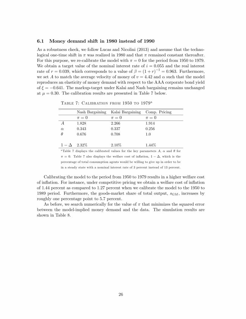
As a robustness check, we follow Lucas and Nicolini (2013) and assume that the techno-logical one-time shift in π was realized in 1980 and that π remained constant thereafter.For this purpose, we re-calibrate the model with π = 0 for the period from 1950 to 1979.We obtain a target value of the nominal interest rate of i = 0.055 and the real interestrate of r = 0.039, which corresponds to a value of β = (1 + r)−1 = 0.963. Furthermore,we set A to match the average velocity of money of v = 4.42 and α such that the modelreproduces an elasticity of money demand with respect to the AAA corporate bond yieldof ξ = −0.641. The markup-target under Kalai and Nash bargaining remains unchangedat µ = 0.30. The calibration results are presented in Table 7 below.

Table 7: Calibration from 1950 to 1979a

Nash Bargaining Kalai Bargaining Comp. Pricingπ = 0 π = 0 π = 0

A 1.828 2.266 1.914α 0.343 0.337 0.256θ 0.676 0.708 1.0

1−∆ 2.32% 2.10% 1.44%aTable 7 displays the calibrated values for the key parameters A, α and θ for

π = 0. Table 7 also displays the welfare cost of inflation, 1 − ∆, which is the

percentage of total consumption agents would be willing to give up in order to be

in a steady state with a nominal interest rate of 3 percent instead of 13 percent.

Calibrating the model to the period from 1950 to 1979 results in a higher welfare costof inflation. For instance, under competitive pricing we obtain a welfare cost of inflationof 1.44 percent as compared to 1.27 percent when we calibrate the model to the 1950 to1989 period. Furthermore, the goods-market share of total output, sGM , increases byroughly one percentage point to 5.7 percent.

As before, we search numerically for the value of π that minimizes the squared errorbetween the model-implied money demand and the data. The simulation results areshown in Table 8.

26

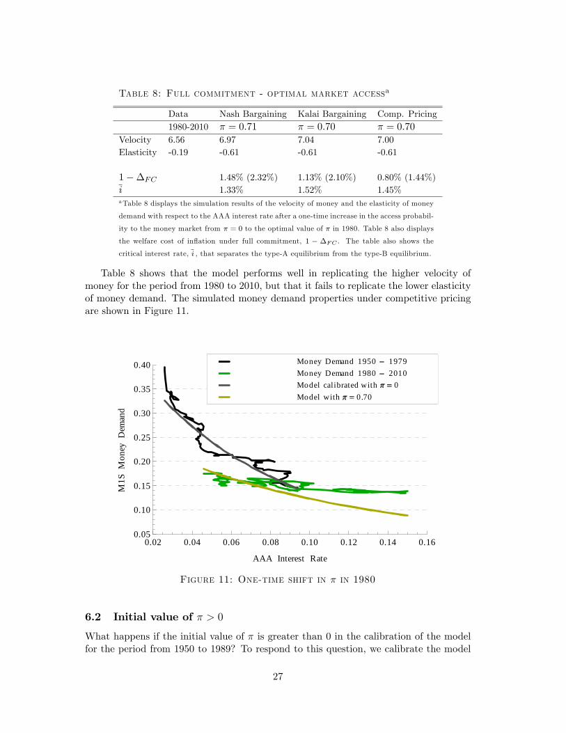
Table 8: Full commitment - optimal market accessa

Data Nash Bargaining Kalai Bargaining Comp. Pricing1980-2010 π = 0.71 π = 0.70 π = 0.70

Velocity 6.56 6.97 7.04 7.00Elasticity -0.19 -0.61 -0.61 -0.61

1−∆FC 1.48% (2.32%) 1.13% (2.10%) 0.80% (1.44%)i 1.33% 1.52% 1.45%aTable 8 displays the simulation results of the velocity of money and the elasticity of money

demand with respect to the AAA interest rate after a one-time increase in the access probabil-

ity to the money market from π = 0 to the optimal value of π in 1980. Table 8 also displays

the welfare cost of inflation under full commitment, 1 − ∆FC . The table also shows the

critical interest rate, i , that separates the type-A equilibrium from the type-B equilibrium.

Table 8 shows that the model performs well in replicating the higher velocity ofmoney for the period from 1980 to 2010, but that it fails to replicate the lower elasticityof money demand. The simulated money demand properties under competitive pricingare shown in Figure 11.

0.02 0.04 0.06 0.08 0.10 0.12 0.14 0.160.05

0.10

0.15

0.20

0.25

0.30

0.35

0.40

AAA Interest Rate

M1S

Mon

eyD

eman

d

Model with 0.70Model calibrated with 0Money Demand 1980 2010Money Demand 1950 1979

Figure 11: One-time shift in π in 1980

6.2 Initial value of π > 0

What happens if the initial value of π is greater than 0 in the calibration of the modelfor the period from 1950 to 1989? To respond to this question, we calibrate the model

27

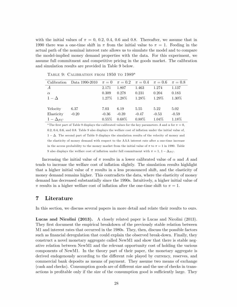
with the initial values of π = 0, 0.2, 0.4, 0.6 and 0.8. Thereafter, we assume that in1990 there was a one-time shift in π from the initial value to π = 1. Feeding in theactual path of the nominal interest rate allows us to simulate the model and to comparethe model-implied money demand properties with the data. For this experiment, weassume full commitment and competitive pricing in the goods market. The calibrationand simulation results are provided in Table 9 below.

Table 9: Calibration from 1950 to 1989a

Calibration Data 1990-2010 π = 0 π = 0.2 π = 0.4 π = 0.6 π = 0.8

A 2.171 1.807 1.463 1.274 1.137α 0.309 0.278 0.231 0.204 0.1831−∆ 1.27% 1.28% 1.28% 1.29% 1.30%

Velocity 6.37 7.03 6.19 5.55 5.22 5.02Elasticity -0.20 -0.36 -0.39 -0.47 -0.53 -0.591−∆FC 0.55% 0.68% 0.88% 1.04% 1.18%aThe first part of Table 9 displays the calibrated values for the key parameters A and α for π = 0,

0.2, 0.4, 0.6, and 0.8. Table 9 also displays the welfare cost of inflation under the initial value of,

1 −∆. The second part of Table 9 displays the simulation results of the velocity of money and

the elasticity of money demand with respect to the AAA interest rate after a one-time increase

in the access probability to the money market from the initial value of π to π = 1 in 1990. Table

9 also displays the welfare cost of inflation under full commitment with π = 1, 1−∆FC .

Increasing the initial value of π results in a lower calibrated value of α and A andtends to increase the welfare cost of inflation slightly. The simulation results highlightthat a higher initial value of π results in a less pronounced shift, and the elasticity ofmoney demand remains higher. This contradicts the data, where the elasticity of moneydemand has decreased substantially since the 1990s. Intuitively, a higher initial value ofπ results in a higher welfare cost of inflation after the one-time shift to π = 1.

7 Literature

In this section, we discuss several papers in more detail and relate their results to ours.

Lucas and Nicolini (2013). A closely related paper is Lucas and Nicolini (2013).They first document the empirical breakdown of the previously stable relation betweenM1 and interest rates that occurred in the 1980s. They, then, discuss the possible factorssuch as financial deregulation that could explain the observed break-down. Finally, theyconstruct a novel monetary aggregate called NewM1 and show that there is stable neg-ative relation between NewM1 and the relevant opportunity cost of holding the variouscomponents of NewM1. In the theory part of their paper, the monetary aggregate isderived endogenously according to the different role played by currency, reserves, andcommercial bank deposits as means of payment. They assume two means of exchange(cash and checks). Consumption goods are of different size and the use of checks in trans-actions is profitable only if the size of the consumption good is suffi ciently large. They

28

find that the new monetary aggregate performs as well on low and medium frequenciesduring the period 1915-2008, as was the case with M1 for the period 1915-1990.

At the time of our writing, we had no access to their new monetary aggregate NewM1.

Faig and Jerez (2007). Our paper is also closely related to Faig and Jerez (2007) whostudy money demand and money velocity in a search model with villages, where moneyis necessary for goods transactions. They assume that buyers are subject to idiosyncraticpreference shocks, and only a fraction of them (1− θ) can readjust their money holdingsbefore trading in the goods market. This generates a role for the precautionary demandof money. Using United States data from 1892 to 2003, Faig and Jerez (2007) show thatthe demand for money and the welfare cost of inflation decreased dramatically at theend of the sample. In Table 3, they show that the welfare cost of inflation was 0.15percent in 2003 as opposed to 1 percent for most of the 20th century.17 Their estimatesof θ are decreasing over time with θ being equal to 1 in 1892 and 0.139 in 2003. Theyalso document that the demand for precautionary balances almost halved in the lastpart of the sample, being 47 percent in 2003 as opposed to over 80 percent for all thepreceding years, while the velocity of money showed an upward trend over the secondhalf of the past century.

Our model differs from Faig and Jerez (2007) in several dimensions. We also con-sider limited commitment while they assume full commitment. As shown above, limitedcommitment and full commitment lead to different theoretical results, and the estimatesdiffer quantitatively as well. Agents’preferences and the matching technology are alsodifferent in both papers. Faig and Jerez (2007) assume that agents are matched with cer-tainty in the goods market, while we allow for the possibility of them being unmatched.They assume that buyers are subject to preference shocks, while we abstract from thispossibility. The two papers also differ in terms of the monetary aggregate used in thedata. We use M1 adjusted for retail sweep accounts, while they use M1 minus the cur-rency held abroad. Finally, Faig and Jerez (2007) focus on competitive search in thegoods market, while we consider Nash, Kalai, and competitive pricing. Our results arequalitatively similar to theirs. However, we find that the drop in the welfare cost ofinflation, due to financial innovation, is smaller than the one reported by them.

Berentsen, Menzio and Wright (2011, BMW hereafter). In the extension sec-tion, BMW introduce bilateral trade credit into the Lagos and Wright (2005) frameworkto investigate whether this modification can account for the observed downward shift inmoney demand. They find that it can account for this to a large extent, but that theelasticity of money demand moves into the wrong direction. To replicate the effects ofbilateral trade credit, we perform the same experiment as BMW. That is, we assumethat until 1990 the probability that a bilateral meeting between a buyer and a seller isnon-anonymous is zero; note that bilateral credit is feasible in non-anonymous meetings.After 1990, the probability that such a meeting is non-anonymous is π = 0.28 (see Figure12). The value of π = 0.28 is chosen numerically, such that the squared error between

17When deriving the welfare cost of inflation, Faig and Jerez (2007) consider an increase of the inflationrate from 0 percent to 10 percent.

29

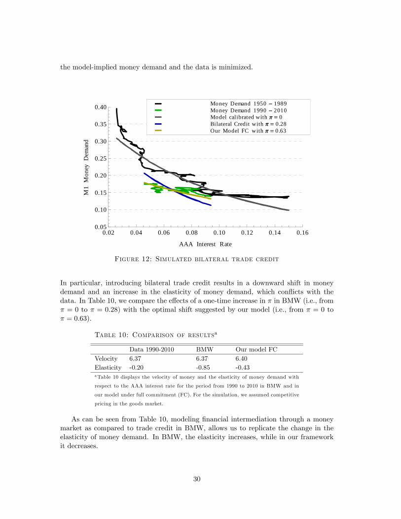
the model-implied money demand and the data is minimized.

0.02 0.04 0.06 0.08 0.10 0.12 0.14 0.160.05

0.10

0.15

0.20

0.25

0.30

0.35

0.40

AAA Interest Rate

M1

Mon

eyD

eman

d

Our Model FC with 0.63Bilateral Credit with 0.28Model calibrated with 0Money Demand 1990 2010Money Demand 1950 1989

Figure 12: Simulated bilateral trade credit

In particular, introducing bilateral trade credit results in a downward shift in moneydemand and an increase in the elasticity of money demand, which conflicts with thedata. In Table 10, we compare the effects of a one-time increase in π in BMW (i.e., fromπ = 0 to π = 0.28) with the optimal shift suggested by our model (i.e., from π = 0 toπ = 0.63).

Table 10: Comparison of resultsa

Data 1990-2010 BMW Our model FCVelocity 6.37 6.37 6.40Elasticity -0.20 -0.85 -0.43aTable 10 displays the velocity of money and the elasticity of money demand with

respect to the AAA interest rate for the period from 1990 to 2010 in BMW and in

our model under full commitment (FC). For the simulation, we assumed competitive

pricing in the goods market.

As can be seen from Table 10, modeling financial intermediation through a moneymarket as compared to trade credit in BMW, allows us to replicate the change in theelasticity of money demand. In BMW, the elasticity increases, while in our frameworkit decreases.

30

Reynard (2004). Reynard (2004) studies the stability of money demand in the UnitedStates using cross-sectional data. In particular, he relates the evolution of financial mar-ket participation to the downward shift in the money demand and its higher interest rateelasticity observed in 1970s. Agents who participate in the financial market can holdboth money and non-monetary assets (NMA), whereas the latter are assets that can beconverted into money by paying a transaction cost – example of NMA are certificates ofdeposits, stocks, and bonds. Agents who do not participate in the financial market canonly hold money. Reynard (2004) shows that an important component of financial mar-ket participation is the household’s real financial wealth, which increased steadily duringthe 1960s and 1970s, and that the probability of holding NMA is positively related to thehousehold’s wealth. He then uses the measure of asset market participation to estimatethe stability of money demand. He finds that, as real wealth and the opportunity costof holding money increased during the 1970s, a higher portion of the population decidedto participate in the financial market and hold part of the wealth in NMA. This shiftedthe interest rate elasticity of money demand upwards since only agents who participatein the financial market can adjust their portfolio of money and NMA when interest rateschange. Thus, using cross-sectional data, Reynard (2004) concludes that the moneydemand remains stable during the post war period, while previous time-series studies"inappropriately" suggest instability and their estimates of the interest rate elasticityare "flawed".

Teles and Zhou (2005). Teles and Zhou (2005) also observe that the stable relation-ship between M1 and the interest rate broke down at the end of the 1970s. Their viewis that M1 is no longer a good measure of the transaction demand for money after 1980.Before 1980, there was a clear distinction between M1 and M2: M1 could be used fortransactions and did not yield any rate of return, while M2 offered a positive rate ofreturn but could not be used for transactions. Since 1980, this distinction vanished dueto changes in regulation, development of electronic payments, and the introduction ofretail sweep programs. Teles and Zhou (2005) show that an appropriate measure of thetransaction demand for money after 1980 is provided by the money zero maturity aggre-gate (MZM). This money aggregate includes financial instruments that can be used fortransaction immediately at zero cost. They show that the long run relationship betweenthe money demand and the interest rate is restored when M1 is used for the period1900-1979 and MZM for the period 1980-2003.

Ireland (2009). Lucas’s (2000) quantifies the welfare costs of inflation. Ireland (2009)revisits the Lucas’s (2000) results by using new data made available from 1995 to 2006.This is the period where intensive sweep retail programs have been introduced by severelydistorting the role of M1 as a measure of the transaction demand for money. Due to thechange in the nature of M1, a new aggregate, M1RS, has been used in Ireland’s (2009)estimations; M1RS is computed by adding the value of sweep funds into M1. To isolatethe recent behavior of the money demand, Ireland (2009) focuses on two subperiods,1980-2006 and 1900-1979. He shows that the relation between M1RS and the interestrate remains stable in the period after 1980, but that relationship looks different thanthat highlighted by Lucas (2000). He finds that the modest growth of M1RS observed in

31

earlier data can be better explained by a semi-log specification of the money demand, asopposed to the log-log specification proposed by Lucas (2000). Furthermore, the interestrate elasticity of the money demand seems to be much lower in 1980-2006 than what itused to be from 1900 to 1979. Both these changes lead to estimates of the welfare costof inflation which are lower than those in Lucas (2000).

VanHoose and Humphrey (2001). VanHoose and Humphrey (2001) study the ef-fect of the introduction of retail sweep accounts on bank reserves and the ability of theFederal Reserve to conduct monetary policy. In particular, they investigate the effect oflower required reserve balances on funds rate volatility and monetary policy in a modelof optimal bank reserve management. They document that the introduction of retailsweep accounts that began in 1993 reduced the required bank reserves at the FED by70 percent. Theoretically, VanHoose and Humphrey show that lower bank reserves havean ambiguous effect on the fund rate volatility. On the one hand, lower reserve require-ments reduce sensitivity of the demand for reserves and funds borrowing to variationsin the Fed funds rate, which makes the funds rate more volatile. On the other hand,lower reserve requirements, increase, for any level of total reserve balances, the portionof reserves the banks can use to cover unexpected payments, which ultimately reducethe overnight funds demand and so the volatility of the overnight funds rate. As a result,the composite effect of lower reserve balances on the funds rate volatility is ambiguous.Moreover, the higher Fed funds rate volatility, which may be triggered by the reducedreserve balances, can be transmitted to the yield curve and raise the volatility of theshort-term interest rate, thereby affecting the effectiveness of monetary policy. Empir-ically, VanHoose and Humphrey test for this possibility. They find that lower reservebalances increase the short-term interest rate volatility only before the period where theFed publicly announced the target of the funds rate. After the funds rate target wasannounced, the effect of lower reserve requirements on the short-term interest rates wasnot significant.

Baumol-Tobin cash-management models. The impact of financial innovation onmoney demand and money velocity has been also studied using Baumol-Tobin cash-management models (e.g., Attanasio, Guiso and Jappelli, 2002, and Alvarez and Lippi,2009).18 Using micro data from an Italian survey from 1989 to 1995, Attanasio, Guisoand Jappelli (2002) study the implication of the Automated Teller Machine (ATM) cardadoption on money demand, interest and the expenditure elasticity of money demand,and the welfare cost of inflation. They show that the interest-rate elasticity for house-holds with an ATM card is twice as large as it is for households which do not possessone, i.e., −0.59 as opposed to −0.27 (Table 3, p.331). Overall, they estimate a welfarecost of inflation that equates to 0.06 percent of nondurable consumption. They alsoshow that the welfare cost of inflation is higher for households with an ATM card (0.09

18Some recent extensions of Baumol (1952) and Tobin (1956) have studied exogenous versus endoge-nous market segmentation (Alvarez, Atkeson and Edmond, 2009, and Chiu, 2012). In these models,agents decide to transfer the money from the goods market to the credit market periodically. As aresult, only a fraction of them are able to trade in the credit market at a given point in time. Theseworks do not investigate the effect of financial innovation on the precautionary demand for money.

32

percent) than for households without (0.05 percent), and that it is declining over timefor each household’s type (Table 4, p.339).

Using the same data set from 1993 to 2004, Alvarez and Lippi (2009) estimate theeffect of ATM card use on money demand in a model with random withdrawal arrivalrates. They estimate an interest rate elasticity of money demand equal to 0.43 forhouseholds with ATM cards, and 0.48 for households without (p. 391).19 They alsoshow that, as a result of the financial innovation, the welfare loss of inflation in 2004 isapproximately 40 percent smaller than it was in 1993 (Table VII, p.394).

Our paper differs from Attanasio, Guiso and Jappelli (2002) and Alvarez and Lippi(2009) in several dimensions. First, our theoretical framework is substantially differentfrom theirs. We build our setup on Lagos and Wright (2005) and extend it to allowagents to lend and borrow cash in a money market before goods transactions take place.Since this is a paper that deals with money demand behavior, we believe it is importantto be explicit about the frictions that make money essential: agent’s anonymity, lack ofdouble coincidence of wants, and lack of public communication. The Lagos and Wrightframework is convenient for our study, since it includes all these frictions in a tractableway. Second, our concept of financial innovation is not related to ATM card use but,instead, focuses on the increasing use of sweep accounts since the 1990s. We claim thatthis innovation, which allows for automatic transfers of excess funds from a checkingaccount into a higher interest-bearing account (typically into a money market fund) hasdramatically changed the demand for money, as well as its interest-rate elasticity, andthe welfare cost of inflation. Third, here, we focus on the possible structural break thatoccurred in money demand and in the interest-rate elasticity of money demand followingthe introduction of the sweep accounts. We test for the structural break using differentsubperiods in the range between 1950 and 2010, for different patterns of participationin the money market. Fourth, like in Lucas (2000) and most of the literature followingLagos and Wright (2005), we use M1, while the studies discussed above use monetaryaggregates that are smaller than M1. (For example, they do not include the moneydemand of firms or interest-bearing bank deposits.) This may explain, in part, why ourestimates of the welfare cost of inflation are substantially higher than theirs.

8 Conclusion

At the beginning of the 1990s the empirical relation between M1 and the movements ininterest rates began to fall apart. In this paper, we ask of what accounts for this shiftand the lower interest-rate elasticity of money demand. To answer this question, weconstruct a microfounded monetary model with a money market. Agents face idiosyn-cratic liquidity shocks which generate an ex-post ineffi cient allocation of the medium ofexchange: some agents will hold cash but have no current need for it, while other agentswill hold insuffi cient cash for their liquidity needs. We find that the money market af-fects money demand via two channels. First, it allows agents who hold cash, but haveno current need for it, to earn interest. Second, it allows agents who hold insuffi cient

19Some previous studies on cross-sectional household data report elasticities smaller than 0.25 (e.g.,Lippi and Secchi, 2009, and Daniels and Murphy, 1994).

33

cash to borrow and, by doing so, reallocates the existing stock of cash more effi ciently.We calibrate the model to U.S. data and find that a one-time increase in the access

probability to the money market at the beginning of the 1990s replicates the behaviorof money demand very well. This result suggests that the emergence of money marketdeposit accounts in the 1980s and the introduction of the sweep technology in the 1990sare responsible for the observed empirical changes in money demand.

34

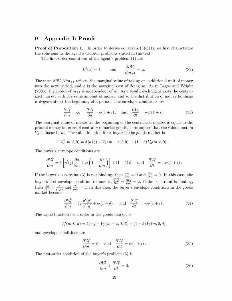
9 Appendix I: Proofs

Proof of Proposition 1. In order to derive equations (8)-(11), we first characterizethe solutions to the agent’s decision problems stated in the text.

The first-order conditions of the agent’s problem (1) are

U ′(x) = 1, andβ∂V1

∂m+1= φ. (32)

The term β∂V1/∂m+1 reflects the marginal value of taking one additional unit of moneyinto the next period, and φ is the marginal cost of doing so. As in Lagos and Wright(2005), the choice of m+1 is independent of m. As a result, each agent exits the central-ized market with the same amount of money, and so the distribution of money holdingsis degenerate at the beginning of a period. The envelope conditions are

∂V3

∂m= φ,

∂V3

∂d= φ (1 + i) , and

∂V3

∂`= −φ (1 + i) . (33)

The marginal value of money at the beginning of the centralized market is equal to theprice of money in terms of centralized market goods. This implies that the value functionV3 is linear in m. The value function for a buyer in the goods market is

V b2 (m, `, 0) = δ [u (q) + V3 (m− z, `, 0)] + (1− δ)V3(m, `, 0).

The buyer’s envelope conditions are

∂V b2

∂m= δ

[u′(q)

∂q

∂m+ φ

(1− ∂z

∂m

)]+ (1− δ)φ, and

∂V b2

∂`= −φ (1 + i) .

If the buyer’s constraint (3) is not binding, then ∂q∂m = 0 and ∂z

∂m = 0. In this case, the

buyer’s first envelope condition reduces to ∂V b2∂m = ∂V3

∂m = φ. If the constraint is binding,then ∂q

∂m = φg′(q) and

∂z∂m = 1. In this case, the buyer’s envelope conditions in the goods

market become

∂V b2

∂m= δφ

u′(q)

g′ (q)+ φ (1− δ) , and

∂V b2

∂`= −φ (1 + i) . (34)

The value function for a seller in the goods market is

V s2 (m, 0, d) = δ [−q + V3 (m+ z, 0, d)] + (1− δ)V3(m, 0, d),

and envelope conditions are

∂V s2

∂m= φ, and

∂V s2

∂d= φ (1 + i) . (35)

The first-order condition of the buyer’s problem (6) is

∂V b2

∂m+∂V b

2

∂`= 0. (36)

35

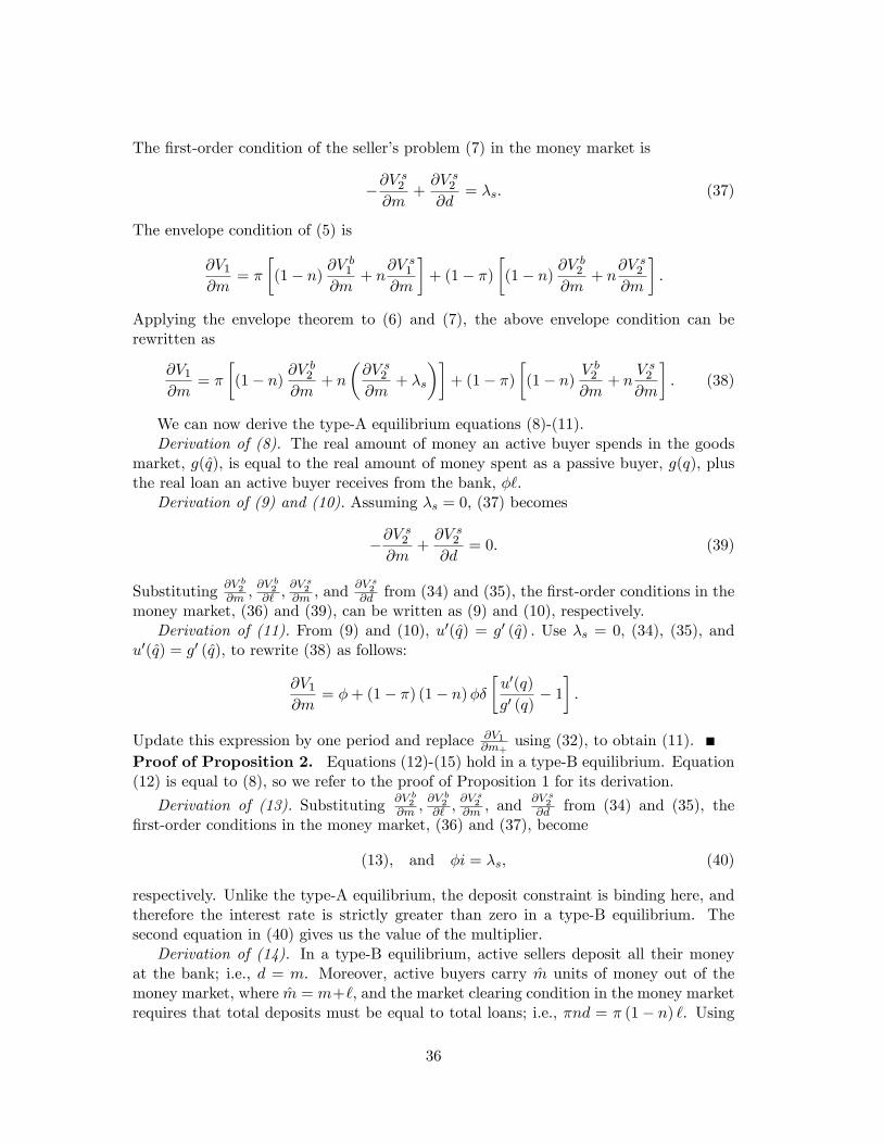
The first-order condition of the seller’s problem (7) in the money market is

−∂Vs

2

∂m+∂V s

2

∂d= λs. (37)

The envelope condition of (5) is

∂V1

∂m= π

[(1− n)

∂V b1

∂m+ n

∂V s1

∂m

]+ (1− π)

[(1− n)

∂V b2

∂m+ n

∂V s2

∂m

].

Applying the envelope theorem to (6) and (7), the above envelope condition can berewritten as

∂V1

∂m= π

[(1− n)

∂V b2

∂m+ n

(∂V s

2

∂m+ λs

)]+ (1− π)

[(1− n)

V b2

∂m+ n

V s2

∂m

]. (38)

We can now derive the type-A equilibrium equations (8)-(11).Derivation of (8). The real amount of money an active buyer spends in the goods

market, g(q), is equal to the real amount of money spent as a passive buyer, g(q), plusthe real loan an active buyer receives from the bank, φ`.

Derivation of (9) and (10). Assuming λs = 0, (37) becomes

−∂Vs

2

∂m+∂V s

2

∂d= 0. (39)

Substituting ∂V b2∂m ,

∂V b2∂` ,

∂V s2∂m , and ∂V s2

∂d from (34) and (35), the first-order conditions in themoney market, (36) and (39), can be written as (9) and (10), respectively.

Derivation of (11). From (9) and (10), u′(q) = g′ (q) . Use λs = 0, (34), (35), andu′(q) = g′ (q), to rewrite (38) as follows:

∂V1

∂m= φ+ (1− π) (1− n)φδ

[u′(q)

g′ (q)− 1

].

Update this expression by one period and replace ∂V1∂m+

using (32), to obtain (11).Proof of Proposition 2. Equations (12)-(15) hold in a type-B equilibrium. Equation(12) is equal to (8), so we refer to the proof of Proposition 1 for its derivation.

Derivation of (13). Substituting ∂V b2∂m ,

∂V b2∂` ,

∂V s2∂m , and ∂V s2

∂d from (34) and (35), thefirst-order conditions in the money market, (36) and (37), become

(13), and φi = λs, (40)

respectively. Unlike the type-A equilibrium, the deposit constraint is binding here, andtherefore the interest rate is strictly greater than zero in a type-B equilibrium. Thesecond equation in (40) gives us the value of the multiplier.

Derivation of (14). In a type-B equilibrium, active sellers deposit all their moneyat the bank; i.e., d = m. Moreover, active buyers carry m units of money out of themoney market, where m = m+`, and the market clearing condition in the money marketrequires that total deposits must be equal to total loans; i.e., πnd = π (1− n) `. Using

36

d = m and m = m + `, the market clearing condition in the money market can berewritten as m = (1− n) m. Multiplying each side of the last equation by φ, and using(4), we obtain (14).

Derivation of (15). Use (40) and the envelope conditions in the goods market, (34)and (35), to rewrite the money market envelope condition (38) as follows

∂V1

∂m= πφ

[δu′(q)

g′ (q)+ 1− δ

]+ (1− π)φ

{(1− n)

[δu′(q)

g′ (q)+ 1− δ

]+ n

}.

Finally, update this expression by one period and replace ∂V1∂m+

using (32), to obtain (15).

Proof of Lemma 1. Since a buyer has to work to repay his debt, he may default in thecentralized market. Here, we derive conditions such that debt repayment is voluntary.In what follows, we denote variables of a defaulting agent (or deviator) with a tilde “∼”.A defaulting buyer’s value function at the beginning of the centralized market is

V3 (m) = U (x∗)− h+ βV+1 (m+1)

and his budget constraint x∗ + φm+1 = h + φm + φT. Note that non-repayment onlyaffects hours of work and the amount of money a buyer takes into the next period. Byeliminating h using the budget constraint, the value function V3 (m) can be rewritten as

V3 (m) = U (x∗)− x∗ − φm+1 + φm+ φT + βV+1 (m+1) .

The value function of a buyer who repays his loan in the centralized market is

V3 (m) = U (x∗)− h+ βV+1 (m+1) ,

and his budget constraint x∗+φm+1 = h+φm+φT −φ (1 + i) `. By eliminating h usingthe budget constraint, we can rewrite V3 (m) as

V3 (m) = U (x∗)− x∗ − φm+1 + φm+ φT − φ (1 + i) `+ βV+1 (m+1) .

A buyer repays his loan if and only if V3 (m) ≥ V3 (m), which implies

φ (1 + i) ` ≤ φm+1 − φm+1 + β[V+1 (m+1)− V+1 (m+1)

]. (41)

Let us now derive V+1 (m+1) and V+1 (m+1).Derivation of V+1 (m+1) . A deviator is banned forever from the money market. The

next-period value function of a deviator is

V+1 (m+1) =1

1− β

[(1− n) δu (q)− nδsq + U (x∗)− h

],

where q ≡ πq + (1− π) q is the expected (or average) quantity he produces if he is aseller; with probability π the buyer he meets is active, in which case he produces q, whilewith probability 1 − π the buyer is passive, in which case he produces q. The first twoterms within brackets are the expected net payoff in the goods market, while the third

37

and fourth terms equal the net payoff in the centralized market. Expected hours of workfor a defector in the centralized market are h = (1− n) hb + nhs, where hb and hs areexpected hours of work of a buyer and a seller, respectively, and are defined as

hb = δ[x∗ + φ+1m+2 − φ+1m+1 − φ+1T+1 + g (q)

]+ (1− δ)

[x∗ + φ+1m+2 − φ+1m+1 − φ+1T+1

]= x∗ + φ+1m+2 − φ+1m+1 − φ+1T+1 + δg (q)

and

hs = δs[x∗ + φ+1m+2 − φ+1m+1 − φ+1T+1 − g

]+ (1− δs)

[x∗ + φ+1m+2 − φ+1m+1 − φ+1T+1

]= x∗ + φ+1m+2 − φ+1m+1 − φ+1T+1 − δsg,

respectively. If the deviator is a seller in the next period, then he receives, in the goodsmarket, an average amount of money, in real terms, equal to g ≡ πg (q) + (1− π) g (q).Hence, using (1− n) δs = nδ, expected hours of work for a deviator can be rewritten as

h = (1− n) hb + nhs

= x∗ + φ+1m+2 − φ+1m+1 − φ+1T+1 + (1− n) δ [g (q)− g] .

Moreover, using m+2 = γm+1 and T+1 = (γ − 1)m+1, we can rewrite h as follows

h = x∗ + (γ − 1)φ+1m+1 − (γ − 1)φ+1m+1 + (1− n) δ [g (q)− g]

= x∗ + (γ − 1) [g (q)− g (q)] + (1− n) δ [g (q)− g] .

Substituting h into V+1 (m+1) yields

V+1 (m+1) =1

1− β

{(1− n) δu (q)− nδsq + U (x∗)− x∗

− (γ − 1) [g (q)− g (q)]− (1− n) δ [g (q)− g]

}.

Derivation of V+1 (m+1). Let u ≡ πu (q) + (1− π)u (q) be the expected utility of anondeviating buyer in the goods market. If the buyer is active, he enjoys utility u (q) ; ifhe is passive, he enjoys utility u (q). The next-period value function of a nondeviator is

V+1 (m+1) =1

1− β {(1− n) δu− nδsq + U (x∗)− h} .

Note that the average disutility, q, suffered by a seller in the goods market depends onhis trading partner’s participation status, active vs passive, and not on his participationstatus. Expected hours of work of a nondeviator in the centralized market are h =(1− n)hb + nhs, where

hb = δ[x∗ + φ+1m+2 − φ+1m+1 − φ+1T+1 + g

]+ (1− δ)

[x∗ + φ+1m+2 − φ+1m+1 − φ+1T+1

]= x∗ + φ+1m+2 − φ+1m+1 − φ+1T+1 + δg

38

and

hs = δs[x∗ + φ+1m+2 − φ+1m+1 − φ+1T+1 − g

]+ (1− δs)

[x∗ + φ+1m+2 − φ+1m+1 − φ+1T+1

]= x∗ + φ+1m+2 − φ+1m+1 − φ+1T+1 − δsg.

Hence, average hours of work for a nondeviator are

h = (1− n)hb + nhs

= x∗ + φ+1m+2 − φ+1m+1 − φ+1T+1

= x∗,

where we have used T+1 = m+2 −m+1. By replacing h in V+1 (m+1), we obtain

V+1 (m+1) =1

1− β {(1− n) δu− nδsq + U (x∗)− x∗} .

Using the above expressions to eliminate V+1 (m+1) and V+1 (m+1) into (41), we obtain

φ (1 + i) ` ≤ φm+1 − φm+1 + β[V+1 (m+1)− V+1 (m+1)

]= γ [φm− φm] +

β

1− β

{(1− n) δ [πu (q) + (1− π)u (q)]

−nδsq + U (x∗)− x∗}

+β

1− β

[− (1− n) δu (q) + nδsq − U (x∗) + x∗

+ (γ − 1) [g (q)− g (q)] + (1− n) δ [g (q)− g]

]or, after further simplification,

φ` ≤ (γ − β) [g (q)− g (q)]

(1 + i) (1− β)

+β (1− n) δ {π [u (q)− g (q)] + (1− π) [u (q)− g (q)]− [u (q)− g (q)]}

(1 + i) (1− β)

where q satisfies (18).Derivation of (18). The envelope condition for a defector in the money market is

∂V1

∂m= (1− n)

∂V b2

∂m+ n

∂V s2

∂m.

which, substituting ∂V b2 /∂m and ∂V s

2 /∂m, can be written as

∂V1

∂m= (1− n)φ

[δu′(q)

g′ (q)+ 1− δ

]+ nφ.

Updating the previous equation one period ahead, and using the first-order condition inthe centralized market, we obtain (18).Proof of Proposition 3. Equations (17), (18), and (20)-(23) hold in a type-0 equi-librium. The derivation of (17) and (18) is in the proof of Lemma 1. The derivation of

39

(20) is in the proof of Proposition 1. Equation (21) is straightforward and means thatthe real loan which a buyer receives from the bank is equal to the maximum amount hecan get. This is a direct consequence of the fact that his borrowing constraint is bindingin the type-0 equilibrium.

Derivation of (22). Let λΦ be the Lagrange multiplier on the buyer’s borrowingconstraint (16). Then, the first-order condition to the buyer’s problem (19) is

∂V b2

∂m+∂V b

2

∂`= λΦ. (42)

The first-order condition of the seller’s problem is (37). If λΦ > 0 and λs = 0, then (42)and (37) can be written as

δ

[u′(q)

g′ (q)− 1

]=λΦ

φ+ i, and (22), (43)

respectively, where we have used (34) and (35) to eliminate ∂V b2∂m ,

∂V b2∂` ,

∂V s2∂m , and ∂V s2

∂d . Thefirst expression in (43) gives us the value of the multiplier λΦ.

Derivation of (23). Use λs = 0 and the envelope conditions in the goods market,(34) and (35), to rewrite the money market envelope condition (38) as follows

∂V1

∂m= φ (1− n) δ

{π

[u′(q)

g′ (q)− 1

]+ (1− π)

[u′(q)

g′ (q)− 1

]}+ φ.

Finally, update this expression by one period and replace ∂V1∂m+

using (32), to get (23).

Proof of Proposition 4. Equations (17), (18), and (24)-(27) hold in a type-I equilib-rium. The derivation of (17) and (18) is in the proof of Lemma 1. Equations (24) and(25) are identical to (20) and (21), respectively. Equation (26) is identical to (14).

Derivation of (27). Use (34) and (35) to substitute ∂V b2∂m and ∂V b2

∂` in (42), and ∂V s2∂m

and ∂V s2∂d in (37) to get

δu′(q)

g′ (q)− δ − i =

λΦ

φand φi = λs, (44)

respectively. Again, eliminate ∂V b2∂m ,

∂V s2∂m , and λs into (38) using (34), (35), and (44),

respectively, to obtain

∂V1

∂m= πφ

{(1− n)

[δu′(q)

g′ (q)+ 1− δ

]+ n (1 + i)

}+(1− π)φ

{(1− n)

[δu′(q)

g′ (q)+ 1− δ

]+ n

}.

Updating this expression by one period, and using (32) to replace ∂V1∂m+1

, we obtain (27).

Proof of Proposition 5. Equations (17), (18), and (28)-(31) hold in a type-IIequilibrium. The derivation of (17) and (18) is in the proof of Lemma 1. Equations (28)and (30) are identical to (20) and (14), respectively.

40

Derivation of (29). In a type-II equilibrium, active sellers deposit all their money(i.e., λs > 0) and the buyer’s borrowing constraint is non-binding (i.e., λΦ = 0). Substi-tuting λΦ = 0 into (42), we obtain

∂V b2

∂m+∂V b

2

∂`= 0. (45)

Then, using (34) and (35) to substitute ∂V b2∂m ,

∂V b2∂` ,

∂V s2∂m , and ∂V s2

∂d in (45) and (37), weobtain

(29), and i =λsφ, (46)

respectively. The second equation just gives us the value of the multiplier λs.

Derivation of (31). Eliminate ∂V b2∂m ,

∂V s2∂m , and λs into (38) using (34), (35), and (46),

respectively, to get

∂V1

∂m= φ

{iπ + (1− π) (1− n) δ

[u′(q)

g′ (q)− 1

]+ 1

}.

Updating this expression by one period, and using (32) to replace ∂V1∂m+1

, we obtain (31).

10 Appendix II: Type III equilibrium

In the main text, we mention the existence of a further equilibrium, called type-IIIequilibrium. A type-III equilibrium has the following properties: active sellers do notdeposit all their money (i.e., λs = 0) and the buyer’s borrowing constraint is non-binding(i.e., λΦ = 0).

Proposition 6 With limited commitment, a type-III equilibrium is a tuple{i, q, q, q, φ`, φ¯

}satisfying (17), (18), and

g(q) = g(q) + φ`, (47)

i = δ

[u′(q)

g′ (q)− 1

], (48)

i = 0, (49)γ − ββ

= (1− π) (1− n) δ

[u′(q)

g′ (q)− 1

]. (50)

The meaning of all equations in Proposition (6) is the same as for their counterpartsin Proposition (5), except that (30) is now replaced by (49). Active buyers consume thefirst-best quantity and the nominal interest rate is zero in a type-III equilibrium.

By comparison of Propositions 6 and 1, it is easy to see that the type-III and type-Aequilibria implement the same allocation. Indeed, in a type-III equilibrium, buyers arenot borrowing-constrained. Hence, relaxing the borrowing constraint does not affecttheir decision.

41

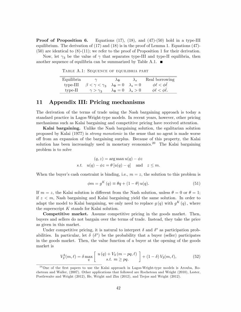
Proof of Proposition 6. Equations (17), (18), and (47)-(50) hold in a type-IIIequilibrium. The derivation of (17) and (18) is in the proof of Lemma 1. Equations (47)-(50) are identical to (8)-(11); we refer to the proof of Proposition 1 for their derivation.

Now, let γ3 be the value of γ that separates type-III and type-II equilibria, thenanother sequence of equilibria can be summarized by Table A.1.

Table A.1: Sequence of equilibria part

Equilibria γ λΦ λs Real borrowingtype-III β < γ < γ3 λΦ = 0 λs = 0 φ` < φ¯

type-II γ > γ3 λΦ = 0 λs > 0 φ` < φ¯.

11 Appendix III: Pricing mechanisms

The derivation of the terms of trade using the Nash bargaining approach is today astandard practice in Lagos-Wright-type models. In recent years, however, other pricingmechanisms such as Kalai bargaining and competitive pricing have received attention.

Kalai bargaining. Unlike the Nash bargaining solution, the egalitarian solutionproposed by Kalai (1977) is strong monotonic in the sense that no agent is made worseoff from an expansion of the bargaining surplus. Because of this property, the Kalaisolution has been increasingly used in monetary economics.20 The Kalai bargainingproblem is to solve

(q, z) = arg maxu(q)− φzs.t. u(q)− φz = θ [u(q)− q] and z ≤ m.

When the buyer’s cash constraint is binding, i.e., m = z, the solution to this problem is

φm = gK (q) ≡ θq + (1− θ)u(q). (51)

If m = z, the Kalai solution is different from the Nash solution, unless θ = 0 or θ = 1;if z < m, Nash bargaining and Kalai bargaining yield the same solution. In order toadapt the model to Kalai bargaining, we only need to replace g (q) with gK (q) , wherethe superscript K stands for Kalai solution.

Competitive market. Assume competitive pricing in the goods market. Then,buyers and sellers do not bargain over the terms of trade. Instead, they take the priceas given in this market.

Under competitive pricing, it is natural to interpret δ and δs as participation prob-abilities. In particular, let δ (δs) be the probability that a buyer (seller) participatesin the goods market. Then, the value function of a buyer at the opening of the goodsmarket is

V b2 (m, `) = δmax

q

[u (q) + V3 (m− pq, `)

s.t. m ≥ pq.

]+ (1− δ)V3(m, `), (52)

20One of the first papers to use the Kalai approach in Lagos-Wright-type models is Arouba, Ro-cheteau and Waller, (2007). Other applications that followed are Rocheteau and Wright (2010), Lester,Postlewaite and Wright (2012), He, Wright and Zhu (2012), and Trejos and Wright (2012).

42

where p is the price, and q the quantity of goods he consumes if he enters the goodsmarket. The first-order condition to this problem is

u′(q) = p (φ+ λq) , (53)

where λq denotes the Lagrange multiplier on the cash constraint, m ≥ pq.The seller’s value function at the opening of the goods market is

V s2 (m, d) = δs max

qs[−qs + V3 (m+ pqs, d)] + (1− δs)V3(m, d). (54)

The first-order condition to this problem is

pφ = 1. (55)

If m > pq, the buyer consumes the effi cient quantity q∗, where q∗ solves u′(q∗) = 1. Ifm = pq, he spends all his money and consumes q < q∗. Note that, in equilibrium, anactive buyer holds more money than a passive buyer. This means that λq > λq. It thenfollows that q > q.

The buyer’s envelope conditions are

∂V b2

∂m= φ

[δu′ (q) + 1− δ

]and

∂V b2

∂`= −φ (1 + i) , (56)

where we have used (33), (53), and (55). Notice the similarity between (56) and (34).The two expressions are the same if θ = 1.

The seller’s envelope conditions are exactly the same as (35); i.e., ∂V s2∂m = φ, and

∂V s2∂d = φ (1 + i).Using the buyer’s budget constraint at equality (i.e., pq = m) and (55) we obtain

φm = gC (q) ≡ q, (57)

where the superscript C stands for competitive pricing.Finally, note that under competitive pricing the goods market clearing condition

holds, i.e.,δ(1− n) [πq + (1− π)q] = δsnqs, (58)

where q (q) is the quantity consumed by a buyer who has (has no) access to the moneymarket.

12 Appendix IV: Data sources

The data we use for the calibration is provided by the U.S. Department of Commerce:Bureau of Economic Analysis (BEA), the Board of Governors of the Federal Reserve Sys-tem (BGFRS), the Federal Reserve Bank of St. Louis (FRBL), and the U.S. Departmentof Labor: Bureau of Labor Statistics (BLS).

43

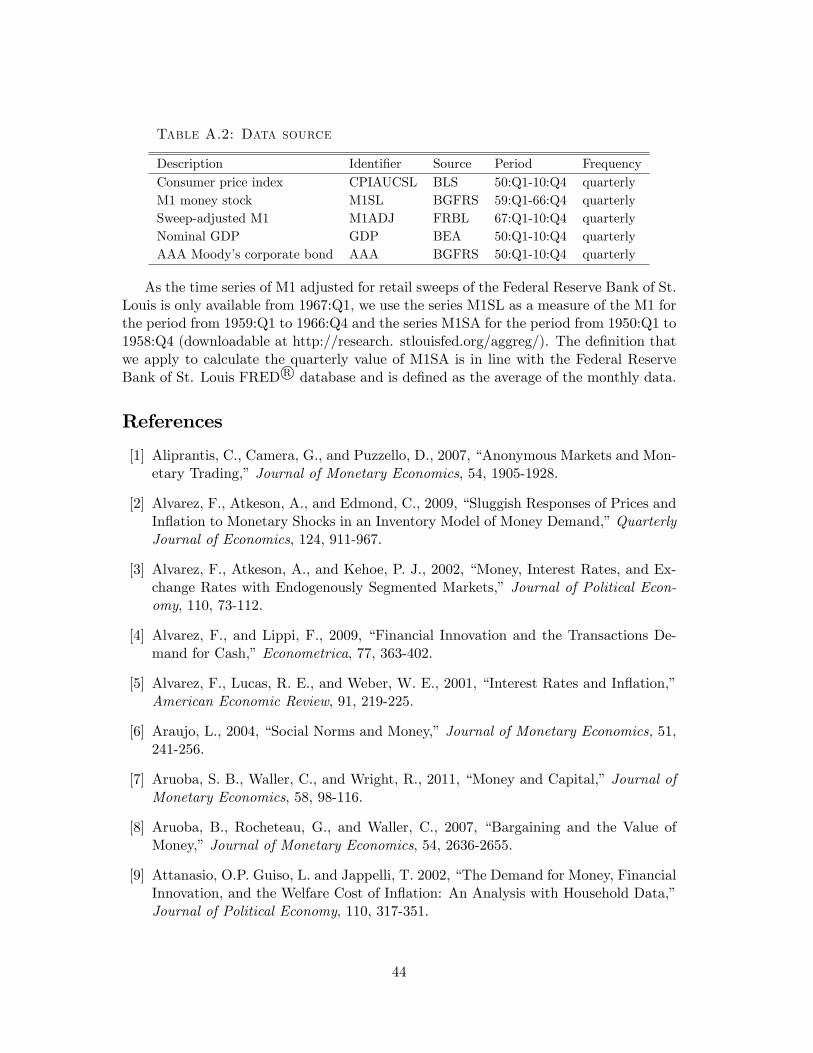
Table A.2: Data source

Description Identifier Source Period FrequencyConsumer price index CPIAUCSL BLS 50:Q1-10:Q4 quarterlyM1 money stock M1SL BGFRS 59:Q1-66:Q4 quarterlySweep-adjusted M1 M1ADJ FRBL 67:Q1-10:Q4 quarterlyNominal GDP GDP BEA 50:Q1-10:Q4 quarterlyAAA Moody’s corporate bond AAA BGFRS 50:Q1-10:Q4 quarterly

As the time series of M1 adjusted for retail sweeps of the Federal Reserve Bank of St.Louis is only available from 1967:Q1, we use the series M1SL as a measure of the M1 forthe period from 1959:Q1 to 1966:Q4 and the series M1SA for the period from 1950:Q1 to1958:Q4 (downloadable at http://research. stlouisfed.org/aggreg/). The definition thatwe apply to calculate the quarterly value of M1SA is in line with the Federal ReserveBank of St. Louis FRED R© database and is defined as the average of the monthly data.

References

[1] Aliprantis, C., Camera, G., and Puzzello, D., 2007, “Anonymous Markets and Mon-etary Trading,”Journal of Monetary Economics, 54, 1905-1928.

[2] Alvarez, F., Atkeson, A., and Edmond, C., 2009, “Sluggish Responses of Prices andInflation to Monetary Shocks in an Inventory Model of Money Demand,”QuarterlyJournal of Economics, 124, 911-967.

[3] Alvarez, F., Atkeson, A., and Kehoe, P. J., 2002, “Money, Interest Rates, and Ex-change Rates with Endogenously Segmented Markets,” Journal of Political Econ-omy, 110, 73-112.

[4] Alvarez, F., and Lippi, F., 2009, “Financial Innovation and the Transactions De-mand for Cash,”Econometrica, 77, 363-402.

[5] Alvarez, F., Lucas, R. E., and Weber, W. E., 2001, “Interest Rates and Inflation,”American Economic Review, 91, 219-225.

[6] Araujo, L., 2004, “Social Norms and Money,”Journal of Monetary Economics, 51,241-256.

[7] Aruoba, S. B., Waller, C., and Wright, R., 2011, “Money and Capital,”Journal ofMonetary Economics, 58, 98-116.

[8] Aruoba, B., Rocheteau, G., and Waller, C., 2007, “Bargaining and the Value ofMoney,”Journal of Monetary Economics, 54, 2636-2655.

[9] Attanasio, O.P. Guiso, L. and Jappelli, T. 2002, “The Demand for Money, FinancialInnovation, and the Welfare Cost of Inflation: An Analysis with Household Data,”Journal of Political Economy, 110, 317-351.

44

[10] Bailey, M., 1956, “The Welfare Cost of Inflationary Finance,”Journal of PoliticalEconomy, 64, 93-110.

[11] Baumol, W. J., 1952, “The Transactions Demand for Cash: An Inventory TheoreticApproach,”Quarterly Journal of Economics, 66, 545-556.

[12] Berentsen, A., Camera, G., and Waller, C., 2007, “Money, Credit and Banking,”Journal of Economic Theory, 135, 171-195.

[13] Berentsen, A., Menzio, G., and Wright, R., 2011, “Inflation and Unemployment inthe Long Run,”American Economic Review, 101, 371-398.

[14] Chiu, J., 2012, “Endogenously Segmented Asset Market in an Inventory-theoreticModel of Money Demand,”Macroeconomic Dynamics, forthcoming.

[15] Chiu, J., and Molico, M., 2010, “Liquidity, redistribution, and the welfare cost ofinflation,”Journal of Monetary Economics, 57, 428-438.

[16] Christopoulou, R., and Vermeulen, P., 2008, “Markups in the Euro Area and theU.S. over the Period 1981-2004,”European Central Bank Working Paper Series 856.

[17] Cooley, T. F., and Hansen, G. D., 1989, “The Inflation Tax in a Real Business CycleModel,”American Economic Review, 79, 733-748.

[18] Cooley, T. F., and Hansen, G. D., 1991, “The Welfare Costs of Moderate Inflations,”Journal of Money, Credit and Banking, 23, 483-503.

[19] Craig, B., and Rocheteau, G., 2008, “Inflation and Welfare: A Search Approach,”Journal of Money, Credit and Banking, 40, 89-120.

[20] Cynamon, B. Z., Dutkowsky, D. H., and Jones, B. E., 2006, “Redefining the Mon-etary Aggregates: A Clean Sweep.”Eastern Economic Journal, 32, 661-673.

[21] Cynamon, B. Z., Dutkowsky, D. H., and Jones, B. E., 2007, "Sweep-AdjustedMonetary Aggregates for the United States." Online document available athttp://www.sweepmeasures.com, December 27, 2007.

[22] Daniels K.N. and Murphy N.B. 1994, “The Impact of Technological Change on theCurrency Behavior of Households: An Empirical Cross Section Study,”Journal ofMoney, Credit and Banking, 26, 867—874.

[23] Faig, M., and Jerez, B., 2005, “A Theory of Commerce,” Journal of EconomicTheory, 122, 60-99.

[24] Faig, M., and Jerez, B., 2007, “Precautionary Balances and the Velocity of Circu-lation of Money,”Journal of Money, Credit, and Banking, 39, 843-873.

[25] Fischer, S., 1981, “Towards an Understanding of the Costs of Inflation: II,”Carnegie-Rochester Conference Series on Public Policy, 15, 5-42.

45

[26] Friedman, M., 1969, The Optimum Quantity of Money and Other Essays, Aldine,Chicago.

[27] Grossman, S. J. and Weiss, L., 1983, “A Transactions-Based Model of the MonetaryTransmission Mechanism,”American Economic Review, 73, 871-880.

[28] He, C., Wright, R., and Zhu, Y., 2012, “Housing and Liquidity,” working paper,University of Wisconsin-Madison.

[29] Ireland, P. 2009, “On the welfare cost of inflation and the recent behavior of moneydemand,”American Economic Review, 99, 1040-1052.

[30] Kalai, E., 1977, “Proportional Solutions to Bargaining Situations: InterpersonalUtility Comparisons,”Econometrica, 45, 1623-1630.

[31] Kiyotaki, N., and Wright, R., 1993 “A Search-theoretic Approach to MonetaryEconomics,”American Economic Review, 83, 63-77.

[32] Lagos, R., and Wright, R., 2005, “A Unified Framework for Monetary Theory andPolicy Evaluation,”Journal of Political Economy, 113, 463-484.

[33] Lester, B., Postelwaite, A., and Wright, R., 2012, “Information, Liquidity, AssetPrices and Monetary Policy,”Review of Economic Studies, 79, 1209-1238.

[34] Lippi, F. and Secchi, A. 2009, “Technological change and the households’demandfor currency,”Journal of Monetary Economics, 56, 222-230.

[35] Lucas, R., 1981, “Discussion of: Stanley Fischer, Towards an Understanding of theCosts of Inflation: II,”Carnegie-Rochester Conference Series on Public Policy, 15,43-52.

[36] Lucas, R., 2000, “Inflation and Welfare,”Econometrica, 68, 247-274.

[37] Lucas, R. and J.P. Nicolini, 2013, “On the Stability of Money Demand,”mimeo.

[38] Moen, E. R., 1997, “Competitive Search Equilibrium,” Journal of Political Econ-omy, 105, 385-411.

[39] Mortensen, D., and Wright, R., 2002, “Competitive Pricing and Effi ciency in SearchEquilibrium,”International Economic Review, 43, 1-20.

[40] Reynard, S. 2004, “Financial market participation and the apparent instability ofmoney demand,”Journal of Monetary Economics, 51, 1297-1317.

[41] Rocheteau, G., andWright, R., 2005, “Money in Competitive Equilibrium, in SearchEquilibrium, and in Competitive Search Equilibrium,”Econometrica, 73, 175-202.

[42] Rocheteau, G., and Wright, R., 2009, “Inflation and Welfare in Models with TradingFrictions,”in Monetary Policy in Low Inflation Economies, by Ed Nosal and DaveAltig, Cambridge University Press.

46

[43] Rocheteau, G., and Wright, R., 2010, “Liquidity and Asset Market Dynamics,”working paper, University of California, Irvine.

[44] Rojas Breu, M., 2013, “The welfare effect of access to credit,”Economic Inquiry,51, 235-247.

[45] Rotemberg, J. J., 1984, “A Monetary Equilibrium Model with Transactions Costs,”Journal of Political Economy, 92, 40-58.

[46] Silber, W. 1983, “Recent Structural Change in the Capital Markets,”AER Papersand Proceedings, 73, 89-95.

[47] Teles, P. and Zhou, R. 2005, “A stable money demand: Looking for the rightmonetary aggregate,”Federal Reserve Bank of Chicago Economic Perspectives, 29,50-63.

[48] Telyukova, I.A. 2013, “Household Need for Liquidity and the Credit Card DebtPuzzle,”Review of Economic Studies, 80, 1148-1177.

[49] Telyukova, I. A., and Visschers, L., 2012, “Precautionary Demand for Money in aMonetary Business Cycle Model,”Journal of Monetary Economics, forthcoming.

[50] Telyukova, I. A., and Wright, R. 2008, “A Model of Money and Credit, with Appli-cation to the Credit Card Debt Puzzle,”Review of Economic Studies, 75, 629-647.

[51] Tobin, J., 1956, “The Interest-Elasticity of the Transactions Demand for Cash,”Review of Economics and Statistics, 38, 241-247.

[52] Trejos, A., and Wright, R., 2012, “Shi-Trejos-Wright Meets Duffi e-Garleanu-Pedersen,”working paper, University of Wisconsin-Madison.

[53] VanHoose, D.D. and Humphrey, D.B. 2001, “Sweep Accounts, Reserve Manage-ment, and Interest Rate Volatility,” Journal of Economics and Business, 53, 387-404.

47