Embed Size (px)
Citation preview

Financial institutions in crisis:
Modeling the endogeneity between credit risk and capital
requirements∗
Ren-Raw Chen
N. K. Chidambaran
Michael B. Imerman
Ben J. Sopranzetti
This Version: June 2009
JEL Classification: G01; G24; G28; G32
∗ Chen and Chidambaran are at the Graduate School of Business Administration, Fordham Uni-versity. Imerman and Sopranzetti are at the Rutgers Business School - Newark and New Brunswick,Rutgers University. We would like to thank the Whitcomb Center for Research in Financial Servicesfor their generous support. Sopranzetti gratefully acknowledges financial support for the projectprovided by a Faculty Research Grant from Rutgers Business School-Newark and New Brunswick.Contact Author: Ben J. Sopranzetti, Rutgers Business School - Newark and New Brunswick, Pis-cataway, NJ 08854. Email: [email protected]; Phone: (732) 445-4188; Fax: (732)445-2333.
Financial institutions in crisis:
Modeling the endogeneity between credit risk and capital
requirements
ABSTRACT
This manuscript presents a credit-risk-based model for the establishment
of minimum bank capital requirements. The structural model determines the
minimum level of equity required to yield a maximum acceptable cumulative
probability of default given a bank’s existing liability structure. It is based on a
modified version of the Geske (1977) structural model which assumes that new
equity is issued to pay down maturing debt; this is particularly appropriate for
financial institutions in times of distress. The model is traditionally used to
accurately measure the term structure of a firm’s default risk, given its existing
capital structure and its associated market value of equity. This manuscript
demonstrates how Geske can be adapted to use a default probability threshold
as an input and to solve for the corresponding level of equity that yields this
default probability. The model overcomes one of the major pitfalls of current
market-risk-based Basel capital requirements: the lack of inclusion of the firm’s
liability structure. The Geske model, unlike other structural credit risk models
which simplify the liability structure by imposing an arbitrary default bound-
ary, is particularly well-suited for financial institutions because of its ability
to accommodate the complicated bank capital structures that are observed in
reality. The manuscript examines the case of Lehman Brothers, to demonstrate
how the model might be used by regulators as a dynamic tool to accurately
measure default risk, assess bank solvency, and, in turn, to set appropriate
credit-risk-based capital requirements.

1 Introduction
The recent financial crisis that has rocked the global financial system has demon-
strated the need for new tools to measure and manage the risks and capital require-
ments in financial institutions. Marked by the dramatic demise of major Wall Street
icons and a massive bailout of financial services companies, the financial system stands
at a critical juncture. The risk based capital requirements established by Basel II have
proved inadequate in the face of rapidly changing credit risks and market conditions.
Central banks and regulators are grappling with the need to anticipate default and
the capital infusion required to reduce default probability to acceptable levels. Crit-
ical to this task is the quick and accurate measure of default risk reflecting rapidly
changing market conditions. In this paper, we propose a new approach to determine
the level of default risk in financial institutions and show how regulators can use our
measure of default risk to estimate the amount of capital infusion that a financial
institution needs to raise to reduce default probability to acceptable levels.
The financial accords collectively termed as Basel II provide the current framework
for auditing and monitoring bank operations. The First Pillar of these accords, which
specifies the minimum capital requirements for credit, market, and operational risks,
is static and is based on historical analysis of the bank’s balance sheet and operations.
The capital ratio is calculated using the definition of regulatory capital and risk-
weighted assets. Specifically, the requirements mandate that the total capital ratio
must be no lower than 8%. The regulations also specify that Tier 2 capital is limited
to 100% of Tier 1 capital, where Tier 1 and Tier 2 refer to the amount of capital
required against specific instruments held as assets on the bank’s balance sheet. The
primary goal of frameworks such as Basel II is to ensure that banks have a “capital
cushion” to absorb losses and reduce the probability of financial distress and default.
The larger the amount of capital held on the bank’s balance sheet, the lower the
probability of default. The recent financial crisis, and indeed other debacles such
as the S&L crisis in the 1980s, the fall of Long Term Capital Management in the
1990s, have shown that static, asset-based regulatory requirements are ineffective.
Well-known papers such as Koehn and Santomero (1980) and Kim and Santomero
1

(1988) have questioned the use of such static asset-based regulatory ratios which are
incapable of reacting to a fast moving credit environment and changing market risk.
In this paper, we propose a dynamic approach to measuring default risk and
develop regulatory tools to specify capital requirements that keep the probability of
default within an acceptable range. Our approach is based on the Geske (1977) model
and estimates default risk using a contingent claims framework in which equity is a
call option on the underlying assets of the firm. Our approach is along the lines
proposed by Merton (1974) and other structural models, which use the probability
that the call option expires out-of-the-money to measure default probability. Unlike
other structural models, our approach is applicable to firms characterized by large and
complex liability structures and is applicable to estimating default risk in financial
institutions.
Our model provides predictive power of default probability in the sense that it
takes future cash flow obligations and the current market condition as inputs to calcu-
late the probability of bankruptcy over different horizons. Regulators can identify not
only high default risk cases, but also the horizon over which the financial institution
faces the most problems.
Our model also provides the regulator with a prescriptive tool. The financial
institution has several degrees of freedom in controlling default risk. One way is that
the institution can sell assets on the balance sheet and retire debt. Reducing debt
will automatically reduce default risk. However, selling assets may not be desirable
or feasible in illiquid market conditions. The financial institution can also restructure
its debt, i.e. retire debt by issuing new debt in a targeted fashion. The financial
institution can relieve financial constraints caused by a particular cash flow by issuing
new debt with cash flows during periods in which it has financial slack. A better
designed liability structure could therefore ease the cash flow constraints and bring
default probability to acceptable levels. Finally, the financial institution can raise
capital to meet cash flow needs. Of course, the financial institution need not restrict
itself to only one of the above three strategies but can incorporate all the three
methods in a comprehensive approach to manage default risk. Our model can be
2

used to evaluate the impact of any and all these mechanisms and gives regulators
critical insight on whether fresh infusions of capital will (or will not) improve default
risk in any specific case. Our model thus represents a way of merging the monitoring
ability of market participants and the regulator as discussed by Flannery (1998).
We apply our model to understand the implied default risk and capital require-
ments for the case of Lehman Brothers during the Financial Crisis of 2008. We show
that the one year bankruptcy probability reached 50% in April 2008, well before
Lehman Brothers actually failed. We find that volatility plays a crucial role and
that in addition to the market valuation, the level of market uncertainty is critical
in determining default risk. We estimate our model for Lehman Brothers before and
after the capital infusion of $25 Billion and are able to show that this capital was
not sufficient enough to lower its default risk to acceptable levels. Our model thus
shows that capital infusion alone cannot dramatically reduce default risk and Lehman
Brothers required substantial restructuring of its debts and assets in order to reduce
bankruptcy risk.
Our work extends the literature along several dimensions. Our model represents
a liability driven estimation of default risk for a financial institution in contrast to
a static asset driven procedure. The insight that equity markets can be used to
infer default risk parallels the concepts discussed by Black and Scholes (1973) and
Merton (1974) in a single period European option framework. For example, Crosbie
and Bohn (2001) present the KMV model that represents a practical implementation
of the original Black-Scholes-Merton (BSM) approach. This approach to estimating
default risk, however, assumes an exogenously specified default boundary by reducing
the entire liability structure of a firm to a weighted average of two points — short-
term and long-term debt — in order to adhere to the single-period European option
framework. On the other hand, the Geske (1977) approach that underlies our model
endogenously solves for the default boundary over time as a function of the entire
liability structure and the corresponding future cash flows. Financial institutions
have very complex liability structures; over-simplifying the liabilities and using an
exogenously specified default boundary can dramatically distort estimates of credit
3

risk. Our implementation of the Geske (1977) model goes a long way towards realizing
the potential of structural models to generate a practical measure of default risk and
capital requirements to measure and manage the default risk in financial institutions.
Our work also represents a practical implementation of the Geske (1977) model
and incorporates several computational improvements. The computational algorithm
proposed by Geske (1977) requires that the default barrier to be solved for recur-
sively and is difficult to implement. We present an algorithm that does not require
a recursive solution. In our model, the default barrier is instead a direct output of a
binomial model. It has also been shown in the literature that even the simplest term
structure model will highly complicate the solution of the Geske (1977) model. In our
binomial framework, this generalization is straightforward and adds only reasonable
computation time.
Structural models require assumptions regarding how firms deal with intermediate
cash-flow obligations. In our model the firm replaces debt with equity. We note
that alternate models do exist; e.g. the Leland (1994) and Leland and Toft (1996)
models assume that the firm retires debt by issuing more debt. Our model, and the
original Geske (1977) model, are more conservative in assuming that maturing debt
is replaced with equity. This avoids the problem that default risk estimates represent
the impact of future new debt rather than the firm’s current maturity structure.
Further, assuming that debt is replaced with equity ensures that we do not over-
estimate default risk and imposes an additional regulatory constraint on the financial
institution.
Our model allows a capital structure solution to managing default risk and pre-
serving the integrity of the financial institution. There are two important issues in
reducing liabilities. First, which debt does the financial institution retire? Preferably
the financial institution should retire the debt that most constrains the firm. Second,
from where does the financial institution raise the funds to pay down debt? Our
approach can identify the specific debt issues that cause default risk to be high and
the reduction in default risk by replacing the debt with equity.
4

The rest of the paper is as follows. Section 2 reviews the relevant literature.
Section 3 discusses the dataset and methodology employed. Section 4 provides an
overview of the Geske (1977) model framework and a numerical example. Section 5
presents the liability structure and time-line of events for the case of Lehman Brothers.
Section 6 develops estimates of default risk and clearly shows that our model can
accurately predict the higher default risks. Section 7 presents our conclusions and
the policy implications of our work.
2 Related Literature
Several papers have begun to document, examine, and explain the events that led up
to and resulted in the financial crisis. Crouhy, Jarrow, and Turnbull (2008) provide
an in-depth look at the flawed mechanisms driving the “Subprime Crisis of 2007”
from securitization, to capital requirements, and even the role of ratings agencies.
Gorton (2009) explains how the events went from a relatively localized debacle in-
volving derivatives on subprime mortgages to a systemic crisis that engulfed the global
financial system. He attributes the credit crisis to opaque markets, asymmetric infor-
mation, and interconnectedness between financial intermediaries with their collective
exposure to housing prices magnified many times over through the web of complex
contracts. One of the first high-profile victims of the crisis occurred in the UK, with a
run on Northern Rock Bank in September of 2007. This case is profiled by Shin (2009)
where a new type of bank run is described; one that is not only due to liquidity issues
and maturity mismatch but further exacerbated by high leverage. For an excellent
discussion of liquidity and the credit crisis please see Brunnermeier (2009). Central
to the aforementioned papers is the topic of capital adequacy standards. Sadly, the
existing market value risk-based bank capital requirements delineated in Basel II were
not capable of immunizing banks from the perils of credit risk.
There is a rich body of literature that examines the role of bank capital and
relevancy of minimum bank capital adequacy standards for the mitigation of bank
5

risk.1 Diamond and Rajan (2000) offer an explanation for the role of bank capital.
They argue that bank capital makes banks safer and helps avoid distress, which in
turn leads to an increased survival probability: bank capital is important because
“deposits are fragile and prone to runs.” The flip side, however, is that bank capital
reduces liquidity, and one of the primary functions of a bank is its ability to create
liquidity. Since bank capital is crucial to a bank’s survival, Santomero and Watson
(1977) ask the fundamental question of whether or not bank capital levels should be
regulated? Is there an optimal level of bank capital? They find that the optimal
level of bank capital is a trade-off between the cost of bank failures (as a result of
undercapitalization) and the cost of over-capitalization (in terms of the constraints
placed on the bank).
This research on optimal bank capital levels leads to a discussion of bank capital
adequacy and minimum capital requirements. Kareken and Wallace (1978) present
an equilibrium model of banking under different regulatory schemes, two of which
include deposit insurance and capital requirements. 2 They find that capital require-
ments, in and of themselves, do not do much to mitigate bankruptcy risk. Sharpe
(1978) examines the role of bank capital where the bank’s liabilities consist only of
deposits which are insured by a third party, effectively making them risk-free. He
defines capital adequacy in terms of minimizing the insurer’s liability so that it is
“no larger than an insurance premium.” Buser, Chen, and Kane (1981) argue that
capital requirements can serve as an implicit risk-based deposit insurance premium.
Therefore, using their line of reasoning, regulating a bank’s capital levels may be used
in conjunction with a flat-rate deposit insurance scheme to achieve the same results
as one that sets insurance premiums according to risk.
Although Sharpe (1978) indirectly demonstrates that capital adequacy standards
should be risk-based, Koehn and Santomero (1980) formally and directly argue the
1For a comprehensive review of the bank capital regulation literature see Santos (2001).2The literature frequently cites risk-based deposit insurance and minimum capital requirements
as two methods for controlling financial institution risk. Our paper deals with the latter and as suchwe do not discuss the abundant literature on risk-based deposit insurance. For a good review of thisliterature the reader is referred to Allen and Saunders (1993). Also, Santos (2001) does a good jobof expounding the link between deposit insurance and capital requirements as regulatory tools.
6

point. They examine how minimum capital requirements affect banks’ behavior.
Their idea is that a regulator wants to ensure that the bank sets aside enough capital
to keep the probability of failure low (within “acceptable levels”). They demonstrate
that placing restrictions on bank capital might actually have counter-intuitive re-
sults: namely, banks with too much risk may actually become riskier as a result of
stricter capital requirements. Kim and Santomero (1988) extend Koehn and San-
tomero (1980) to include capital requirements that account for the riskiness of the
bank’s portfolio. Hendricks and Hirtle (1997) provide an overview of risk-based capital
requirements and present a case in favor of banks using internal models to determine
regulatory capital, citing that they should “conform more closely to banks’ true risk
exposures”.
The Basel Accords, both I and II, created minimum capital adequacy standards
for banks. The standards were based on market risk; specifically, the riskiness in the
market value of the assets.3 One of the major differences lies in the definition of how
to determine the risks. There are many critiques of the capital adequacy standards set
forth in Basel and with capital adequacy standards in general. We include only the
subset most relevant to our paper here. Thakor (1996) argues that that risk-based
capital requirements can potentially lead to credit rationing. Hellmann, Murdock,
and Stiglitz (2000) also find that capital requirements, by themselves are insufficient
to mitigate bank bankruptcy risk, and that instead they can lead to the perverse
result where banks gamble. Estrella, Park, and Peristiani (2000) claim that simple
capital ratios (specifically, the leverage ratio and gross revenue ratio) are as good or
better at predicting bank failure than risk-weighted Basel-type metrics. Altman and
Saunders (2001) examine two aspects of Basel II risk-based capital regulation, but
find that using agency ratings for the risk-weighting could lead to “cyclically lag-
ging capital requirements” thereby possibly making the financial system less stable
over time. Furthermore, they argue that the current risk-bucketing lacks granular-
ity. As a substitute, they propose a revised weighting system that fits historical
default loss statistics rather closely. Similarly, Krainer (2002) examines alternatives
3For background on Basel II please see Basel Committee on Banking Supervision (2001)
7

to risk-based capital requirements (i.e. full-reserve banking). He proposes a corpo-
rate governance system that reduces the agency problem between creditors/depositors
and stockholders. The optimal contract allows creditors/ depositors to “offset” risk
shifting decisions that may benefit the bank’s shareholders at the creditors’ expense.
Herring (2004) takes a different approach. The paper claims that Basel II stan-
dards and credit risk management best practices cannot be aligned, and offers an
alternative to Basel II: the mandatory issuance of subordinated debt. Kashyap and
Stein (2004) examine the Basel II Internal Ratings Based (IRB) capital requirements
and the effect that it may have on cyclicality in the financial system. They find that
the Basel capital requirements may exacerbate business cycle effects.4
Jarrow (2007) offers an even stronger critique of the Basel II capital requirements;
one that is based on Basel’s lack of concern for credit risk. He argues that Value
at Risk does not account for credit risk appropriately. Kashyap, Rajan, and Stein
(2008) call for a complete overhauling and even rethinking of bank capital regulation,
and propose alternatives including “capital insurance”.
In light of the recent credit crisis and failure of many banking institutions, perhaps
a rethinking of how regulators might set minimum capital standards, especially ones
that take into consideration credit risk, is in order. The first to consider such a
problem is Ronn and Verma (1989). Using an option pricing model, they focus on
deposit insurance, and solve for capital infusion that will lower deposit insurance
premium to a specified level. Our approach differs from Ronn and Verma (1989) in
that we endogenously solve for the market value of debt (they use book value), our
model is dynamic, multi-period with sequential cash flows (theirs is a single period,
static model), and our model uses the bank’s default probability to find the risk-based
capital requirement (theirs uses deposit insurance).
4Interestingly, Pennacchi (2005) argues that risk-based capital requirements are inclined to yieldgreater procyclical effects than risk-based deposit insurance. He, therefore, suggests that Basel IIincorporate some elements of risk-based deposit insurance to help moderate the procyclical natureof the existing framework.
8

2.1 Credit Risk Models: Theory and Applications
Since we employ a credit-risk-based model of capital adequacy our paper is clearly
related to the credit risk literature. Generally speaking, there are two classes of credit
risk models: reduced-form and structural models. The former define default purely
in statistical terms where it is modeled as a jump process with a given intensity,
or hazard rate. Reduced-form models are calibrated to market data and typically
do not take any firm-specific information into account. In this framework default is
unpredictable and the default time is said to be “inaccessible”. Popular reduced-form
models include Jarrow and Turnbull (1995), Duffie and Singleton (1999), Jarrow,
Lando, and Turnbull (1997), and Duffie and Lando (2001).
Our model falls into the structural class. Structural credit risk models view default
as an economic event where firm value declines to a level that is too low to justify
servicing outstanding debt obligations. Structural models originated with Black and
Scholes (1973) where, in their seminal option pricing paper, they noted that when a
firm has debt in its capital structure equity is like a call option on the firm’s unlevered
assets. This idea was later formalized by Merton (1974). In the original BSM frame-
work default can only occur at maturity. If the value of the firm’s assets is not greater
than the face value of the debt then shareholders choose to let the call option expire
(i.e. default) and bondholders do not receive their promised payment but rather take
ownership of the assets. If, however, the value of the firm’s assets is greater than the
face value of the debt then shareholders liquidate the assets and use the proceeds to
pay bondholders with the retaining the residual amount for themselves. The proba-
bility that the call option is not exercised at maturity can be thought of as the default
probability.
Due to the oversimplifying assumptions that underlie the original BSM framework,
the decades that followed would generate many extensions looking to incorporate
more realistic features of debt. One such class of extensions, commonly referred to as
“barrier” structural models, was pioneered by Black and Cox (1976). In their paper
Black and Cox (1976) develop an analytical model for valuing corporate debt with
certain indenture agreements that can result in default occurring before maturity.
9
Specifically, they examine “safety covenants” – contractual provisions that stipulate
the conditions that force restructuring. In the model there is a lower boundary on firm
value, below which the firm is considered “bankrupt”; once the asset value hits this
barrier debtholders take control of the firm’s assets. Longstaff and Schwartz (1995)
develop a model that is a direct extension of Black and Cox (1976). The Longstaff and
Schwartz (1995) model includes stochastic interest rates with a flat, exogenous barrier.
Collin-Dufresne and Goldstein (2001) incorporate mean-reverting leverage ratios into
an exogenous barrier model. Leland (1994) derives a barrier structural model with
endogenous default. The model solves for both the optimal capital structure and the
price of risky debt in the presence of taxes and bankruptcy costs. Leland and Toft
(1996) extend the Leland (1994) model to take debt maturity into account as well.
Distinct from the barrier models is the compound option model of Geske (1977).5
In the Geske model, shareholders own a compound option on the firm’s unlevered
assets. Every time a cashflow is due to bondholders the shareholders must decide
whether to make the payment, effectively exercising the compound option, or default
giving the bondholders (who are the writers of the compound call option) ownership
of the firm’s assets. Default is determined endogenously as a function of the liability
structure and the associated promised cashflows. The Geske model is described in
much greater detail below (see Section 4.1).
Structural models are commonly used for predicting default as they naturally pro-
vide quantitative measures of default probabilities. In the barrier structural models,
default probabilities are given by the first passage time density. In the compound
option model, default probabilities are found by calculating the probability that the
compound option is not going to be exercised at a particular future cash flow time.
This allows us to calculate both the conditional and unconditional default probabili-
ties and actually results in a term structure of default probabilities.
5The Geske compound option model is also derived in a no-arbitrage setting in Geske (1979)where a “leverage effect” is shown to result in nonconstant volatilities. The original Geske (1977)model was also corrected by Geske and Johnson (1984) to properly account for the seniority structureof debt.
10

The KMV model, as described by Crosbie and Bohn (2001), is a modified version
of the original BSM model that is very popular in practice. Using market data as well
as information from a firm’s balance sheet the KMV model calculates expected default
frequencies and the distance to default. Leland (2004) looks at default probabilities
calculated using two structural models – the endogenous barrier model of Leland and
Toft (1996) and the exogenous barrier model of Longstaff and Schwartz (1995) – and
observes how well the predictions fit historical default frequencies. Delianedis and
Geske (2003) compute risk-neutral default probabilities (RNDP) using the original
BSM model and the Geske model. They draw two interesting conclusions that have
very important implications for our model: first, they show that RNDPs serve as an
upper bound to risk-adjusted default probabilities (for both models) and, second, the
Geske model is able to provide important information that other structural models
cannot; specifically, it provides a full term structure of default probabilities. Bharath
and Shumway (2008) compare the distance to default from the BSM/KMV model
with forecasts obtained using a hazard model. Structural credit risk models can also
be used to analyze distress in the financial sector. Mason (2005) uses a real options
approach to model bank failure as the trustee’s optimal decision to liquidate.
3 Methodology
Our approach works as follows. First, we explicitly document the time and dollar
amount of the liability cash flows. This often requires the complete identification of
over a thousand different bonds with their associated coupon and redemption pay-
ments over time. We note that while we had to hand collect the data, the efficiency
of this step can be greatly improved by regulators by requiring that financial institu-
tions provide a detailed breakdown of their liabilities on a weekly, or in the case of a
financial crisis daily, basis to the regulator. This should not be particularly onerous
for the Financial Institutions given that they need to collect the data for internal risk
management purposes.
11

Second, we estimate the market value and volatility of the firm’s equity. In this
paper, we use the most recent price of the financial institutions traded stock and
multiply by the outstanding number of shares to calculate the market capitalization
of the firm as our estimate of market value of equity. For an estimate of equity
volatility, we use the historical standard deviation based on the most recent 30, 60,
and 90 days of traded stock prices. The latest price and the most recent estimate of
volatility allows for the use of measures that incorporate the most relevant information
to estimate the financial health of the financial institution. In dramatically changing
circumstances such as those that exist during a financial crisis, measures that portray
a more stable environment can be misleading.
Third, we construct the default boundary and the term structure of default prob-
abilities. As in the original Geske (1977) model, default is triggered when the value
of the financial institution’s assets fall sufficiently low so as to prevent it from raising
new equity capital. The default boundary is therefore defined as the breakeven point,
or the asset value that sets the current market value of the firm’s equity equal to the
next cash flow obligation. The default probabilities, in conjunction with the endoge-
nous default boundary, provide an accurate and complete picture of the survivability
of the financial institution over both the short-term and the longer-term.
We begin our analysis in January 2008 when Lehman Brothers was in little danger
of default and then evaluate the firm monthly until September when Lehman Brothers
declared bankruptcy. We collect data on the outstanding debt of Lehman Brothers
from the FactSet database. The data in FactSet includes the CUSIP number, the
total face value of the issue, the issue date, the coupon rate, and the maturity date.
Using the Fixed Income Explorer in Factset, we collect all of these data items for
each and every bond as well as the seniority, redemption options, and credit ratings
when available. We identify several thousand bonds issued by Lehman Brothers
and carefully document the outstanding amounts, the coupon rates and maturity of
these bonds taking into account the possibility that the bond has been retired. We
supplement the data on Lehman Brothers debt structure with data from the firms
financial statements (annual income statements from 1998 to 2007, quarterly balance
12

sheets from 3Q.2005 to 4Q.2007, and quarterly cash flows from 3Q.2005 to 4Q.2007).
These data sources allow us to specify in detail the outstanding cash flow obligations
of Lehman Brothers at different horizons. We also estimate the market capitalization
of Lehman Brothers at the end of each month and the historical 30-day and 60-day
volatilities.
We note that we do not include private debt and off-balance sheet obligations
of Lehman Brothers because of a lack of data on these obligations. We offer two
arguments on this front. First, our estimates are necessarily a lower bound on the
true level of default risk. In order to estimate the impact of ignored cash-flow obli-
gations, we re-estimate our model using ad-hoc assumptions on margin requirements
on Lehman’s off-balance sheet activities and the level of private debt. As expected,
the level of default risk rises substantially when additional cash-flow obligations are
incorporated into the model. Second, we note that regulators can demand access
to these data and can easily incorporate the cash-flow liabilities in any real-world
implementation of our model. Indeed, one advantage of our model is the ease with
which additional cash-flows can be incorporated into the analysis when such cash-flow
obligations are deemed to be relevant by the regulators.
4 Model Framework
In this section we discuss our dynamic lattice based structural model for estimating
default risk in financial institutions. Structural models are especially well-suited for
managing and monitoring credit risk, either internally or externally, as they use the
most recent inputs from financial statements and market data. Our approach is based
on the compound option pricing model as developed by Geske (1977) (henceforth
Geske). We first review the Geske model and the related Geske and Johnson (1984)
model. We then present our lattice implementation of the Geske model.
13

4.1 Geske model and Endogenous Default
Structural option pricing methods have been used extensively in the banking litera-
ture to quantify and price deposit insurance (see e.g. Ronn and Verma (1989)) and in
the credit risk literature to estimate default risk (see e.g. Crosbie and Bohn (2001)).
Black and Scholes (1973) and Merton (1974) pioneered the notion that when a firm
has risky debt outstanding, the equity is very much like a call option where share-
holders are faced with the decision to exercise when payment is due to debtholders.
Upon maturity of the debt shareholders can choose to make the payment, effectively
exercising the call option or default by filing for bankruptcy and letting the call option
expire unexercised. In the Merton (1974) approach, the liabilities are modeled as a
fixed point barrier, hence the name barrier structural model, and there is only one
future date in which the exercise decision is made. The firm has the option to default
only at one point - on the final maturity date of the debt. The overly simplistic and
exogenous specification of the default boundary has limited the application of the
Merton approach to estimating default risk, especially for financial institutions.
The Geske (1977) model incorporates multiple cash flows and allows for default at
each time that a cash flow, either a coupon or a face value payout, is due. The Geske
approach thus fundamentally differs in the way it models the default boundary and
the conditions under which the call option is exercised by the shareholders. First,
the Geske approach relaxes the fixed point barrier rendering of the default boundary
to allow for multiple sequential cash flows. Exercising the option to pay a cash flow
due to bondholders delivers to the shareholders a sequence of options corresponding
to the multiple cash flows over the maturity structure of the various components of
debt. Second, the compound option specification evaluates the decision to default at
every cash flow period. Consequently, with the compound option structural model
each and every cash flow is important and the endogenous default barrier is explicitly
a function of these cash flows. Geske (1979) and Geske and Johnson (1984) extended
the basic framework to incorporate a “leverage effect” that causes volatility to change
with leverage and account for the seniority structure of multiple debt claimants. The
14

model is thus especially suited for analyzing default risk in financial institutions and
for estimating bank capital.
Our model is a discrete time implementation of the Geske approach. The en-
dogenous default boundary does make obtaining an analytical solution difficult; we,
however, develop a lattice approach to estimating the default boundary and asset val-
ues. Our discrete time implementation directly solves for the endogenous boundary
without the need for iterative calculations.
The Geske (1977) model and its extensions make several assumptions regarding the
conditions that trigger default, the sequence in which various options are exercised,
and how the equity holders raise the funds needed to exercise the call option and pay
the debtholders. First, the model assumes that the ability to make a cash payment
and the requirement that the market value of the assets is greater than the market
value of future liabilities is important in order to exercise the call option. The default
boundary in these models is therefore endogenous and depends on the market value of
debt and the market value of assets. Second, the model assumes that earlier payments
are more senior to later payments. This naturally leads to the assumption that bonds
with shorter maturities have priority over long maturity bonds, which is consistent
with short-term debt being more important in triggering credit constraints in practice.
Finally, the model assumes that all payments to bondholders are financed by issuing
new equity. This implies that the firm will ultimately become all equity. As a result
the default risk estimated by the model is conservative and is contingent on the firm
being able to raise equity in order to remain solvent. This approach arguably is the
correct approach in the context of financial institution regulation. The focus is on
identifying firms that have an unacceptably high theoretical default risk and require
these firms to restructure by issuing more equity or restructuring its debt in order to
reduce leverage and the associated default risk.
15

4.2 n-Period Geske Model
Let the firms assets evolve according to a diffusion process with dynamics described
by the Stochastic Differential Equation:
dAtAt
= µtdt+ σtdWt (1)
Let Kk denote the current value of a cash flow paid at time Tk. We note that the
value of the cash flow at Tk is also a function of all the cash flows paid prior to time
Tk, that is K1 · · ·Kt−1 . Let A represents the value of the firm’s assets, D represents
the market value of the firms debt, S represents the value of the firm’s equity, r
represents the risk free rate, and σ represents the volatility of the firm’s assets.
D(0, Tk) =∑k
i=1 e−rTiKi[Ni(h
−1 (A1k), · · · , h−i (Aik))−Ni(h
−1 (A1k−1), · · · , h−i (Aik−1))]
+A0[Nk−1(h+1 (A1k), · · · , h+
k−1(Ak−1k−1))−Nk(h+1 (A1k), · · · , h+
k (Akk))]
(2)
where,
h±i (Aij) =lnA(0)− ln Aij + (r ± 0.5σ2Ti)
σ√Ti
(3)
Aij for i < j is the internal solution for A(Ti) to the following equation:
A(Ti) =∑j
k=iD(Ti, Tk) (4)
Note that D(Ti, Ti) = Ki = Aii and that N0(.) = 1 and N1(.) = 1 are i-dimensional
Gaussian probability functions.
We need to solve for Aij sequentially in a process similar to bootstrapping. We
start the second to last period, k − 1. There is one critical value to solve: A(t−1)k
which is the solution to:
Ak−1 = Kk−1 +D(Tk−1, Tk) (5)
16

where,
D(k − 1, k) = Ak−1
(1−N1
(lnAk−1−lnKk+(r+0.5σ2)∆t
σ√
∆t
))(6)
+e−r∆tKkNk
(lnAk−1−lnKk+(r+0.5σ2)∆t
σ√
∆t
)This gives the solution to A(k−1)k as a function of Kk−1 and Kk and other parameters
such as risk free rate and volatility. Then we move backwards one period to k − 2.
In this period, we need to solve for A(k−2)(k−1) and A(k−2)k. The former (A(k−2)(k−1))
can be solved the same way as A(k−1)k since it is a one period bond as a function of
Kk−2 and Kk−1. The latter (A(k−2)k) is more complex. It is a solution to:
Ak−2 = Kk−2 +D(Tk−2, Tk−1) +D(Tk−2, Tk) (7)
where,
D(Tk−2, Tk) = e−2r∆t
∫ ∞Ak−1k
E[min{Ak, Kk}] + e−r∆t∫ Ak−1k
Kk−1
E[Ak−1 −Kk−1] (8)
and hence ¯A(k−2)k is a function of Kk−2, Kk−1, and Kk as well as ¯A(k−1)k which must
be solved first. As we work backwords in the lattice, all the critical values Aij for
i < j are solved.
The total value of debt is:
∑n
k=1D(0, Tk) = A(0)[1−Nn(h+
1 (X1n), · · · , h+n (Xnn))] (9)
+∑n
i=1e−rTiKkNn(h+
1 (X1n), · · · , h+n (Xnn))
The quasi-closed form solution for the n-period Geske model involves n-dimensional
cumulative normal distribution functions. Since this cannot be computed analytically
we have to use a numerical methods. We use a binomial lattice method to implement
the Geske model along the lines of Eom, Helwege, and Huang (2004).
17
4.3 The Lattice Model
The Geske (1977) model involves an endogenous default boundary and we develop a
lattice approach to implement the model. Consider a 6-period binomial lattice model
for the value of the firm’s assets as shown in Figure 1. The shareholders of the firm
have three exercise decisions to make, i.e. there are three cash flows K1, K2, and K3
that they have to make to debt holders. K3 is the debt face value at the final node
and K1 and K2 are debt cash flows at the intermediate nodes. As shown in the figure,
there is an intermediate node In between any two of the cash-flows.
The option to default can be exercised at the nodes a cash flow payment is due.
That is, we model bankruptcy as the option shareholders have to not make a payment
to the debt holders and continue the firm for at least the time interval to the next cash
flow. The decision to exercise the option to default takes into account the relative
value of the assets and the debt of the firm and, as discussed above, is equivalent to a
call option. If the shareholders choose not to make a payment, the firm is in default
and the default boundary refers to the asset value for which the shareholders will
exercise the option to default at different points in time in the lattice. Equivalently,
the default boundary represents the “cut off” asset values below which the firm is
in default at each time t. We estimate the default boundary, debt value, and equity
value by backward recursion in the tree.
An important assumption we make is the source of the funds shareholders use
to meet the cash flow obligation and keep the firm alive until the next cash flow
period. Following Geske (1977) we assume that the shareholders issue new equity at
the current market price to raise the required capital. This assumption simplifies the
calculations and has several implications which we believe makes it especially suitable
to the setting of highly levered financial institutions. First, the transaction reduces
the amount of debt and increases the amount of equity as time evolves, thereby
decreasing the default risk over time. The largest default risk, therefore, arises from
meeting the next cash flow payment. This is typically true of financial institutions
that rely heavily on trust and reputation in the marketplace; failing to make a near-
term cash flow obligation has disastrous consequences. Second, the model will be
18

conservative in estimating default probabilities and unlikely to imply onerous capital
requirements for financial institutions with longer-term cash flow obligations rising
from debt issues, which can usually be refinanced.6
Consider the final nodes at the end of the lattice. On the date of the final con-
tractual cash flow, i.e. terminal time T , the firm liquidates. Since equity is a call
option on the assets, the value to equity holders and the optimal exercise decision is
given by,
ET = max{AT −K3, 0} (10)
where ET is the equity value at the terminal time T , AT is the asset value at the
terminal time T and K2 is the final redemption value of debt. In the above diagram,
the solid dots represent economic states where the equity has positive value and those
hollow dots represent those states where the equity has no value.
Moving backwards along the lattice, the equity value is computed as the risk
neutral expectation of the values in the next period, that is Et = Et[e−r∆tEt+1] for
any t in between any two cash flows.
Consider the second-to-last cash flow K2. At this time, the firm decides if it should
pay down the debt with equity. If the equity value is more than the cash obligation,
then it is rational for the firm to pay down the debt and continue to survive; otherwise,
the debt holders will seize and liquidate the firm, and the equity becomes worthless.
That is: Et = max{Et[e−r∆tEt+1]−K2, 0}
There are two important quantities we compute in the lattice. One is the default
boundary and the other is the survival (default) probability. The default boundary
is the critical value above which the asset value must stay in order for the firm to
remain alive. In the Geske (1977) notation, it is Ai,i+1, which is the highest critical
value at any given time i. If the asset price at time i, Ai, falls below this value the
equity would become worthless. Note that at the critical value the total value of
6We can easily modify the assumption and have the firm issue debt to finance the cash flow pay-ment. This is the assumption underlying the Leland and Toft (1996) model. The model essentiallyimplies a flat default boundary and does not take into account the potential to reduce default riskby raising capital when needed.
19

outstanding debts is equal to the asset value. Above this critical value, the firm can
issue new equity to pay down the debt due at time i. The above definition of default
boundary is effective for all i.
The other quantity of great importance is the survival probability. In the original
Geske (1977) model, as well as in our model, the survival probability is the probability
that the asset value stays above the default boundary. That is,
Q(0, i) = Pr(A1 > A12 ∩ A2 > A23, · · · , Ai > Aii+1) (11)
This joint probability is easy to compute within the lattice. We simply trace each path
in the lattice and count only those that survive. Note that the default probability
between any two cash flow periods is:
Q(0, i− 1)−Q(0, i) (12)
This means that to compute the ith default probability, the firm must survive
until year i− 1 and then default in year i. The associated recovery values are rather
difficult to obtain in an integration format in the original Geske and yet is rather easy
to obtain in the lattice. Similar to the computation of the survival probability, we
trace defaults along the lattice. We then compute the expected value of the assets,
equity, and debt.
4.4 Numerical Example
To demonstrate with a numerical example, consider a firm with annual cash flows 10,
20, and 75 at t = 1, 2, 3 respectively. There is one intermediate node between cash
flows, i.e. ∆t = 0.5,. Let A0 = 300, σ = 10%, r = 3%, . Using the standard binomial
model, we have: u = eσ√δt = 1.0733 and d = e−σ
√δt = 0.9317 . The probabilities are
p = er∆t−du−d = 0.5891 and 1− p = 0.4109.
Figure 2 shows the asset value binomial tree. Figure 3A, 3B, and 3C respectively
shows the three time periods, working backwards from the last time step, represent-
20

ing the equity value taking into account the optimal decision to not make the debt
payment and declaring bankruptcy (shown as zero values in the lattice).
From Figure 3, the value of equity at t = 0 is equal to 27.40. Since asset value
is $300, the resulting debt value is 272.60. To compute the survival probability, we
trace survival through the lattice, i.e. wherever the value of equity is greater than 0.
For the first cash flow, survival occurs at the asset values of 57.57 and 17.06. The
probability is equal to π2 + 2π(1−π) and is equal to 83.12%. Similarly, in the second
year, the survival probability is 74.94%, and 70.00% in the third year. The default
probabilities are therefore 16.88%, 8.18%, and 4.94% in Years 1, 2, and 3 respectively.
The default boundary is also obtained by tracing the lattice. For example, in
Year 1, default occurs in the bottom state, i.e. the state with the lowest asset value.
Hence, the default boundary must in between 300 and 260.44. We note that this
seems to be a rather large range, but as the time period (and step size) shrinks the
gap will narrow and converge. We assume that the firm defaults at the average of the
asset values where the firm just survives and the firm just defaults, e.g. the bottom
two nodes in Year 1. In Year 2, the bottom two states default and top three states
survive. Hence, the default boundary falls in between 300 and 260.44. In Year 3, the
default boundary falls between 300 and 260.44, but this time we know for sure it is
275, the last coupon. The default boundary curve is therefore: 280.22, 280.22, and
275 at Year 1, 2, and 3 respectively.
To compute the expected recovery value of the ith bond (cash flow), we need to
compute E0
[e−riAiIA1>A12∩A2>A23···Ai−1>Ai−1i∩Ai<Aii+1
]. For the three years, we obtain
the following values from the lattice: 42.67 that is composed of 1.64 of the first bond
(out of face value 10), 3.18 of the second bond (out of face value 20), and 37.85 (out of
face value 275). Note that the survival probability of the first year is 83.12%. Hence,
for the first bond, its coupon value is: $10× 0.8312× exp(−5%) = $8.07. Combining
this with its recovery value gives a total value of: $8.07 + 1.64 = $9.71, which is
effectively a risk free bond. Similarly, the second bond has a coupon value of 14.12
and a recovery value of 4.72. Combining these together gives a value of 18.84, which
is also a risk free bond. We also note that for the second bond the recovery value of
21

4.72 comes from 3.18 in the first year and 1.54 in the second year, if the shareholders
default. Finally, for the last bond (face value 275), he first year has a recovery of
37.85, the second year has a recovery of 18.51, and third year has a recovery of 11.77,
for a total recovery value of 68.13. The coupon value is 175.92. Therefore, the total
bond value is 244.05. In terms of yield, the third year bond has a yield-to-maturity
of 3.98% yield, showing a spread of 98 basis points.
5 Lehman Brothers: An Anatomy of a Financial
Crisis
We implement our approach to analyze the default risk for Lehman Brothers lead-
ing up to the firm’s failure. Lehman Brothers was a major financial institution that
experienced severe financial problems disastrous enough that the Wall Street power-
house was forced to file bankruptcy. Figure 4 shows a time line of events at Lehman
Brothers. In this section, we show that our model accurately predicts the substantial
increase in default risk for Lehman Brothers over the first few months of 2008 and we
examine whether capital infusions alone could have prevented bankruptcy.
5.1 The Liabilities
We compile a comprehensive data set representing the liabilities of Lehman Brothers
using the FactSet database. FactSet aggregates financial data from various sources
which allowed us to analyze the firm’s capital structure at extremely detailed levels,
specifically looking into the debt profile of Lehman Brothers. In particular, FactSet
allows us to collect data on every single debt issuance at any given point in time. The
dataset includes basic information of the bonds in FactSet such as the CUSIP number,
the total face value of the issue, the issue date, the coupon rate, and the maturity
date. In addition, it also includes other detailed information such as the “Status”
(matured/redeemed/active), redemption options (callable/putable/convertible), the
redemption date (where applicable), the ratings as per Moodys and S&P, the coupon
22

type (fixed/floating/etc.), and the seniority from the Fixed Income Explorer. This
specific data regarding the debt structure was supplemented with data from the firms
financial statements (annual income statements from 1998 to 2007, quarterly balance
sheets from 3Q.2005 to 4Q.2007, and quarterly cash flows from 3Q.2005 to 4Q.2007).
This permits us to study Lehman Brothers through September 2008, right before it
filed for bankruptcy.
We collate the debt of Lehman by calendar year and estimate the dollar value
of Lehman’s debt in each calendar year. Table 3 details the notional amount of the
liabilities maturing in each calendar year as of January 2008. As seen in the table,
Lehman has substantial amount of debt maturing in the short term in 2008 and 2009.
The table also shows other details of the debt outstanding.
Figure 5 displays the debt maturity structure as of each month in 2008. The
figure shows the notional debt value for each month. As the figure shows, short-
term debt maturing in one to three years and long-term debt with maturities greater
than or equal to 20 years dominate in Lehman’s liability structure. This is typical
for a financial institutions that use short-term debt for working capital needs and
finance their core activities using long-term debt. Figure 5 also shows that the short-
term debt increased dramatically in March of 2008, around the time that the market
realized that Lehman was in financial trouble and did not have enough assets to meet
its financial liabilities.
Figure 5 presents the level of debt at the beginning of each month in 2008. Both
the time at which the liability structure is determined and the time period over which
different tranches of debt are collated can be changed. For example we can calculate
the debt profile every week or every fortnight and collate the liabilities over six-month
windows. Our choice here represents a compromise between the level of detail and
clarity of presentation and does not affect any of our results.
23

5.2 Market Value Inputs
Our model uses two market-determined inputs for calculating the default probability
of Lehman Brothers. The first is the market value of Lehman’s equity and the second
is the volatility of stock returns on Lehman’s.
Figure 6 shows the book value and the market value of Lehman Brothers. The
market value of equity is calculated as the product of the closing stock price on the
estimation day and the number of shares outstanding on that day. The book value
of equity is as reported by COMPUSTAT. As the figure shows, the market value of
equity had a precipitous decline over 2008. In February the equity value dropped from
$35.1 billion to $26.8 Billion, a drop of 23.6%. As Figure 4 shows, the financial crisis
reflected in this dramatic drop in equity value led Lehman to raise additional funds
in March 2008. Lehman obtained a $2 billion 3 year credit line from a consortium of
40 banks including JPMorgan Chase and Citigroup. The infusion stabilized Lehman
over the next two months; however a reported loss of $2.8 Billion in May led to a
further stock price decline of 27.9% in May as shown in the figure.
Figure 7 shows the historical 30-day stock return volatility for Lehman. We cal-
culate the volatility as the annualized standard deviation of Lehman’s daily stock
returns over the prior 30-day period. We use the most recent period to focus on
the most recently available market information of Lehman’s stock returns. As Fig-
ure 7 shows, the volatility estimate spiked in March 2008 reflecting the increase in
uncertainty in February.
5.3 Default Probability
We use the hand collected data on the liability structure, the equity market value, and
the volatility estimates to determine the endogenous default boundary for Lehman
Brothers at the beginning of each month for the period from January 2008 to Septem-
ber 2008.
24

Figure 8 shows the market value and book value of Lehman’s debt. The book
value of debt is the cumulative dollar value of Lehman’s debt from FactSet. The
market value of debt is as estimated by our model. As Figure 8 shows, the market
value of debt is substantially lower than its book value indicating a high default risk
premium for the debt.
Figure 9 shows our model estimates of the 2-year default probability. Default
probability spiked in March 2008 to well over 50% after staying low in January and
February of 2008. Thus, our model predicts the dramatic rise in default risk for
Lehman Brothers, well before the September 2008 bankruptcy filing. The short-term
funds obtained by Lehman did lower the default risk substantially in May and June. In
fact, the default probability was lower than the default probability in April, possibly
because the market anticipates a government intervention and a rescue package.
Figure 10 shows the cumulative default probability over time for Lehman Brothers
at the beginning of each month in 2008. As seen in the figure, the cumulative default
probability is upward sloping with a steep slope in the initial period and the default
probability quickly reaches the highest value. The picture of cumulative probability
is typical for the Geske model and the intuition behind the behavior of cumulative
default is as follows. Financial institutions are characterized by having large amounts
of liabilities, a substantial amount of which typically matures in the short term. The
present value of debt is therefore high and in adverse market conditions a financial
institution faces higher default risk in the short term. The initial rise in default prob-
ability captures the degree of financial distress faced by the financial institution. If
the financial institution does not default in the initial period, the model assumes that
the firm raises equity to meet the debt obligation. This lowers the default probability
in the future periods and results in the cumulative default probability that levels off
in the future periods. We note that the results in Figure 10 reinforce the results from
Figure 9 in that the default risk is the highest for Lehman during March 2008 when
the firm faced financial distress and there was a high degree of uncertainty regarding
whether the government would play a role in supporting financial institutions.
25

6 Managing Default Risk
In this section, we discuss the implications of our model and present how our model
can be used to manage default risk in financial institutions using the case of Lehman
Brothers as an illustration.
The pattern of default probability over time show in Figure 10 has important
implications for the management of default risk in financial institutions. As shown
in the figure, default risk rises initially and levels off for longer term. The pattern
of default probability is a function of the liability structure of financial institutions
and the assumptions made by the model on capital structure changes when liabilities
come due. We argue that these features are important in measuring and managing
default risk in financial institutions. Financial institutions are saddled by a large
amount of financial liabilities and a substantial fraction of these liabilities are due in
the short-term. It is therefore not surprising that the per-period default is the highest
in the initial period and is lower in the later periods. Further, the model’s assumption
that debt is retired using equity further mitigates default risk in later periods.
Our model indicates that the largest threat to the survival of a financial institution
is in the short term. Regulators have to be especially vigilant when the short-term de-
fault risk is unusually high, as for example when the default risk for Lehman brothers
rose to over 50% in April 2008.
We next examine how default risk changes for varying capital structure. Figure 11
graphs default risk as a function of volatility for two different levels of equity capital
in April 2008. The top line shows default risk for Lehman as existed with a market
value leverage ratio of 72.7%. The bottom line shows the default probability at a
market value leverage ratio of 10.4%. As Figure 10 shows, given market conditions as
of April 2008, Lehman would need to dramatically lower leverage in order to reduce
default risk to acceptable levels. In other words, the elasticity of default probability
with respect to market value leverage is fairly low, indicating that default risk can be
lowered substantially only by large infusions of equity capital.
26

The implications for managing default risk in financial institutions are profound.
Our model validates the Federal Reserve’s focus on the short-term viability of financial
institutions and provides tools that the Fed (and other regulators) can use to evaluate
institutions in dramatically changing market conditions. However, the model also
predicts that in adverse market conditions, tweaking the firm’s capital to reach the
magic 8% ratio required by the Basel II accord, would not result in substantially
lowering default risk. Regulators and management at financial institutional have to
fundamentally rethink the operating model when the firm is in a crisis.
7 Conclusions
In this paper we develop and present a new approach to estimating the default risk
of Financial Institutions. Our model is based on the Geske (1977) framework for
valuing compound options and allows for the accurate estimation of default risk, with
an endogenous default boundary, and works for even complex portfolio of liabilities as
is typical for financial institutions. Our model can be readily applied to estimate the
default risk of financial institutions and gives regulators a powerful dynamic tool that
reflects current market conditions in managing default risk of financial institutions.
While an options based approach using structural models has been advocated as
a way to estimate default risk since the seminal work of Black and Scholes (1973)
and Merton (1974), the application to financial institutions has several practical im-
pediments. Traditionally, such structural models have used a single point equivalent
of a firm’s liabilities and have used exogenously imposed default barriers. Our model
considers the entire liability structure and uses an endogenous default boundary to
develop accurate estimates of default risk.
Our model uses the most recent market based inputs, specifically market value of
equity and the volatility of stock returns to estimate default risk. We implement our
model for the first few months of 2008 to the case of Lehman Brothers. We use hand
collected data from FactSet to determine the firm’s detailed liability structure and
daily stock data to estimate market value of equity and stock return volatility. We
27

show that default risk spiked to over 50% in April 2008, well before the bankruptcy
filing by Lehman Brothers in September of 2008.
We show that financial institutions such as Lehman Brothers are characterized
by rapidly rising default risk in the short term that then levels off over the longer
term. The pattern of cumulative default probability has important implications for
the regulation of financial institutions. Our model validates the Federal Reserve’s
focus on the short-term survival probability of a financial institution as the ability to
meet the large short-term cash flows is the most critical. However we also show that
in times of financial crisis when the short-term default risk is very high, a rather large
level of capital infusion is required to increase survival probability. Small levels of
capital infusions do not eliminate risk as illustrated by the case of Lehman Brothers:
default risk remained high following the capital infusion in April 2008.
Our model represents a powerful predictive and diagnostic tool that will enable
regulators to accurately estimate default risk and analyze the impact of any interven-
tion. Moreover our model uses the most recent market data, as opposed to the static
default risk measures that use book values. This is crucial when facing fast moving
market conditions such as those that exist in the midst of a financial crisis.
28

References
Allen, Linda, and Anthony Saunders, 1993, Forbearance and valuation of deposit
insurance as a callable put, Journal of Banking and Finance 17, 629–643.
Altman, Edward I., and Anthony Saunders, 2001, An analysis and critique of the
bis proposal on capital adequacy and ratings, Journal of Banking and Finance 25,
25–46.
Basel Committee on Banking Supervision, 2001, The New Basel Accord: an explana-
tory note (Bank for International Settlements).
Bharath, Sreedhar T., and Tyler Shumway, 2008, Forecasting default with the merton
distance to default model, Review of Financial Studies 21, 1339–1369.
Black, Fischer, and John C. Cox, 1976, Valuing corporate securities: Some effects of
bond indenture provisions, Journal of Finance 31, 351.
Black, Fischer, and Myron Scholes, 1973, The pricing of options and corporate liabil-
ities, Journal of Political Economy 81, 637.
Brunnermeier, Markus K., 2009, Deciphering the liquidity and credit crunch of 2007-
2008, Journal of Economic Perspectives 23, 77–100.
Buser, Stephen A., Andrew H. Chen, and Edward J. Kane, 1981, Federal deposit
insurance, regulatory policy, and optimal bank capital, Journal of Finance 36,
51–60.
Collin-Dufresne, Pierre, and Robert S. Goldstein, 2001, Do credit spreads reflect
stationary leverage ratios?, Journal of Finance 56.
Crosbie, Peter J., and Jeffrey R. Bohn, 2001, Modeling default risk, (KMV, LLC, San
Fransisco, CA).
Crouhy, Michel, Robert A. Jarrow, and Stuart M. Turnbull, 2008, The subprime
credit crisis of 2007, The Journal of Derivatives.
29

Delianedis, Gordon, and Robert Geske, 2003, Credit risk and risk neutral default
probabilities: Information about rating migrations and defaults, EFA 2003 Annual
Conference Paper No. 962.
Diamond, Douglas W., and Raghuram G. Rajan, 2000, A theory of bank capital,
Journal of Finance 55, 2431–2465.
Duffie, Darrell, and David Lando, 2001, Term structures of credit spreads with in-
complete accounting information, Econometrica 69, 633–664.
Duffie, Darrell, and Kenneth J. Singleton, 1999, Modeling term structures of default-
able bonds, Review of Financial Studies 12.
Eom, Young Ho, Jean Helwege, and Jing Zhi Huang, 2004, Structural models of
corporate bond pricing: An empirical analysis, Review of Financial Studies p.
499544.
Estrella, Arturo, Sangkyun Park, and Stavros Peristiani, 2000, Capital ratios as pre-
dictors of bank failure, Economic Policy Review 6.
Flannery, Mark J., 1998, Using market information in prudential bank supervision:
A review of the u.s. empirical evidence, Journal of Money, Credit and Banking 30,
273–305.
Geske, Robert, 1977, The valuation of corporate liabilities as compound options,
Journal of Financial and Quantitative Analysis 12, 541–552.
, 1979, The valuation of compound options, Journal of Financial Economics
7, 63–81.
, and H. E. Johnson, 1984, The valuation of corporate liabilities as compound
options: A correction, Journal of Financial and Quantitative Analysis 19, 231.
Gorton, Gary, 2009, The subprime panic, European Financial Management 15, 10–46.
Hellmann, Thomas F., Kevin C. Murdock, and Joseph E. Stiglitz, 2000, Liberaliza-
tion, moral hazard in banking, and prudential regulation: Are capital requirements
enough?, American Economic Review 90, 147 – 165.
30

Hendricks, Darryll, and Beverly Hirtle, 1997, Bank capital requirements for market
risk: The internal models approach, Economic Policy Review 3.
Herring, Richard J., 2004, The subordinated debt alternative to basel ii, Journal of
Financial Stability 1, 137 – 155.
Jarrow, Robert A., 2007, A critique of revised basel ii, Journal of Financial Services
Research 32, 1 – 16.
, David Lando, and Stuart M. Turnbull, 1997, A markov model for the term
structure of credit risk spreads, The Review of Financial Studies 10, 481–523.
Jarrow, Robert A., and Stuart M. Turnbull, 1995, Pricing derivatives on financial
securities subject to credit risk, The Journal of Finance 50, 53–85.
Kareken, John H., and Neil Wallace, 1978, Deposit insurance and bank regulation:
A partial-equilibrium exposition, Journal of Business 51, 413–438.
Kashyap, Anil K., Raghuram G. Rajan, and Jeremy C. Stein, 2008, Rethinking capital
regulation, in Maintaining Stability in a Changing Financial System Jackson Hole,
Wyoming. Federal Reserve Bank of Kansas City.
Kashyap, Anil K., and Jeremy C. Stein, 2004, Cyclical implications of the basel ii
capital standards, Economic Perspectives 28, 18 – 31.
Kim, Daesik, and Anthony M. Santomero, 1988, Risk in banking and capital regula-
tion, Journal of Finance 43, 1219–1233.
Koehn, Michael, and Anthony M. Santomero, 1980, Regulation of bank capital and
portfolio risk, Journal of Finance 35, 1235–1244.
Krainer, Robert E., 2002, Banking in a theory of the business cycle: a model and cri-
tique of the basle accord on risk-based capital requirements for banks, International
Review of Law and Economics 21, 413 – 433.
Leland, Hayne E., 1994, Corporate debt value, bond covenants, and optimal capital
structure, The Journal of Finance 49, 1213–1252.
31

, 2004, Predictions of default probabilities in structural models of debt, Jour-
nal of Investment Management.
, and Klaus Bjerre Toft, 1996, Optimal capital structure, endogenous
bankruptcy, and the term structure of credit spreads, Journal of Finance 51, 987–
1019.
Longstaff, Francis A., and Eduardo S. Schwartz, 1995, A simple approach to valuing
risky fixed and floating rate debt, The Journal of Finance 50, 789–819.
Mason, Joseph R., 2005, A real options approach to bankruptcy costs: Evidence from
failed commercial banks during the 1990s, Journal of Business 78, 1523–1553.
Merton, Robert C., 1974, On the pricing of corporate debt: The risk structure of
interest rates, The Journal of Finance 29, 449:470.
Pennacchi, George G., 2005, Risk-based capital standards, deposit insurance, and
procyclicality, Journal of Financial Intermediation 14, 432–465.
Ronn, Ehud I., and Avinash K. Verma, 1989, Risk-based capital adequacy standards
for a sample of 43 major banks, Journal of Banking and Finance 13, 21–29.
Santomero, Anthony M., and Ronald D. Watson, 1977, Determining an optimal cap-
ital standard for the banking industry, Journal of Finance 32, 1267–1282.
Santos, Jo A. C., 2001, Bank capital regulation in contemporary banking theory: A
review of the literature, Financial Markets, Institutions and Instruments 10, 41.
Sharpe, William F., 1978, Bank capital adequacy, deposit insurance and security
values, Journal of Financial and Quantitative Analysis 13, 701–718.
Shin, Hyun Song, 2009, Reflections on northern rock: The bank run that heralded
the global financial crisis, Journal of Economic Perspectives 23, 101–119.
Thakor, Anjan V., 1996, Capital requirements, monetary policy, and aggregate bank
lending: Theory and empirical evidence, Journal of Finance 51, 279–324.
32

Figure 1: Lattice model implementation of the Geske model
33

Figure 2: Numerical Example - 3-period Asset Binomial Tree
34

Figure 3: Numerical Example:Equity Values in a Discrete 3-period Binomial Tree
Figure 3B
Figure 3A
Figure 3C
35

Figure 4: Lehman Brothers Time Line
36

Figure 5: Lehman Brothers Debt Maturity
Figure 5 shows the dollar level of debt maturing in each year from 2008 to 2038for Lehman Brothers. Data is shown monthly for the period from January 2009 toSeptember of 2008.
37

Figure 6: Lehman Brothers Equity Value
Figure 6 shows the book value and the market value of equity for LehmanBrothers at the beginning of each month from Jan 2008 to September 2008. Marketvalue of equity is calculated as the product of the stock price multiplied by thenumber of shares outstanding and is represented by the solid line. Book value ofequity is as reported in COMPUSTAT, The market value of equity is one of themarket determined inputs for our model.
38

Figure 7: Lehman Brothers Volatility
Figure 7 shows the historical 3-month volatility by at the beginning of eachmonth from Jan 2008 to September 2008. Historical volatility is calculated byannualizing the standard deviation of daily returns over the prior 3-month period.The data on volatility is the second market determined input for our model.
39

Figure 8: Lehman Brothers Debt Value
Figure 8 shows the book value and the market value of outstanding debt ofLehman Brothers at the beginning of each month from Jan 2008 to September2008.e. Book value of debt represents the cumulative dollar total of debt outstandingfor Lehman Brothers as reported by FactSet. Market value of debt is estimated byour model.
40

Figure 9: Lehman Brothers Default Probability
Figure 9 shows the cumulative 2-year default probability at the beginning ofeach month from Jan 2008 to September 2008 as estimated by our model.
41

Figure 10: Lehman Brothers Cumulative Default Probability
Figure 10 shows the cumulative probability of default through 2028 which isthe longest date debt in our sample. The cumulative default probability is at thebeginning of each month from Jan 2008 to September 2008 as estimated by ourmodel.
42

Figure 11: Lehman Brothers One-Year Default Probability
Figure 11 shows the default probability of Lehman Brothers in April 2008 asa function of equity volatility. In April, Lehman had a market cap of $24,448,000,000and equity volatility of 157%. Our model indicates that the one-year defaultprobability was 46.29% (and the two-year default probability was 36.46% (not shownin the figure). The market value leverage ratio (D/A) is 72.7%. The bottom lineshows the impact of adding equity. As the graph shows, Lehman Brothers canreduce default probability to 5%, but this requires that Lehman substantially lowerits leverage to 10.5%.
43

Table 1: Geske Model Vs KMV
Table 1 reports the values of the default probability for the Lattice model and for the KMVmodel for three different scanrios. In each scenario, Asset Value=300, σ = 0.1. ColumnOne on each panel shows the time of the cash flow, Column Two shows the magnitude ofthe cash flow, Column 3 shows the default probability for the Lattice model, and ColumnFour shows the default probability for the KMV model.
Year Cashflow Geske KMV
Panel A: Even Cashflows1 100 0.828 0.9992 100 0.828 0.9783 100 0.828 0.769
Panel B:⋃
-shaped Cashflows1 100 0.905 0.9992 50 0.905 0.9783 150 0.905 0.769
Panel C:⋂
-shaped Cashflows1 100 0.777 0.9992 150 0.777 0.9783 50 0.777 0.769
44

Table 2: Time Line of Events at Lehman Brothers
• 2007- Jan. 2008: Lehman scales back mortgage business, cutting thousands of
mortgage-related jobs and closing Mortgage origination units
• Q4 2007: Lehman Brothers shows $886 million in quarterly earnings (flat com-
pared to 3rd quarter); reported earnings of $4.192 billion for 2007 fiscal year (a
5% increase from the previous fiscal year)
• Jan. 29, 2008: Lehman announces increase in dividends and plans to repurchase
up to 100 million shares of common stock
• Q1 2008: Lehman Brothers increases holding of Alt-A mortgages despite the
prevailing troubles in the real-estate market
• March 14, 2008: Lehman obtains $2 billion 3 year credit line from consortium
of 40 banks including JPMorgan Chase and Citigroup
• March 14, 2008: Federal Reserve and JPMorgan Chase begin to put together
deal to bail out Bear Stearns
• March 16, 2008: JP Morgan announces offer to purchase Bear Stearns for $2/
share
• March 18, 2008: Lehman shares surged up almost 50% after Federal Reserve
gives investment banks access to the discount window
• April 1, 2008: Lehman looks to raise $4 billion in new capital via an offering of
perpetual convertible preferred stock
• Q2 2008: Lehman Brothers shows a $2.8 billion loss the first loss in the firms
history as a public firm; admits losses came not only from mortgage-related
positions but also from hedges against those positions
• June 9, 2008: Lehman Brothers announces plan to raise addition $6 billion in
new capital ($4 billion in common stock, $2 billion in mandatory convertible
preferred stock)
45
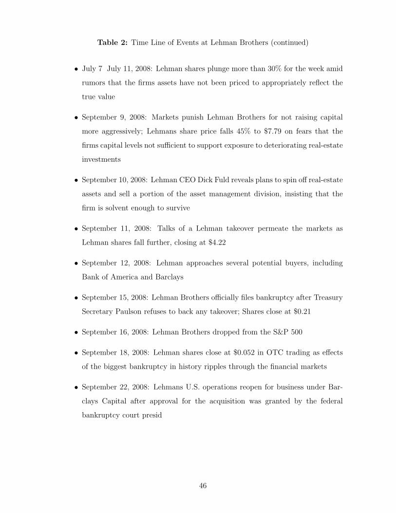
Table 2: Time Line of Events at Lehman Brothers (continued)
• July 7 July 11, 2008: Lehman shares plunge more than 30% for the week amid
rumors that the firms assets have not been priced to appropriately reflect the
true value
• September 9, 2008: Markets punish Lehman Brothers for not raising capital
more aggressively; Lehmans share price falls 45% to $7.79 on fears that the
firms capital levels not sufficient to support exposure to deteriorating real-estate
investments
• September 10, 2008: Lehman CEO Dick Fuld reveals plans to spin off real-estate
assets and sell a portion of the asset management division, insisting that the
firm is solvent enough to survive
• September 11, 2008: Talks of a Lehman takeover permeate the markets as
Lehman shares fall further, closing at $4.22
• September 12, 2008: Lehman approaches several potential buyers, including
Bank of America and Barclays
• September 15, 2008: Lehman Brothers officially files bankruptcy after Treasury
Secretary Paulson refuses to back any takeover; Shares close at $0.21
• September 16, 2008: Lehman Brothers dropped from the S&P 500
• September 18, 2008: Lehman shares close at $0.052 in OTC trading as effects
of the biggest bankruptcy in history ripples through the financial markets
• September 22, 2008: Lehmans U.S. operations reopen for business under Bar-
clays Capital after approval for the acquisition was granted by the federal
bankruptcy court presid
46

Table 3: Lehman Brothers Debts as January 2008 (Million)
Maturity Notional2007 75412008 159312009 119312010 85642011 88532012 74032013 48052014 22172015 21852016 12342017 18612018 6172019 592020 1562021 4282022 3312023 1722024 562025 1202026 43
2027+ 1336Grand Total 75843
Coupon Type Notional Seniority NotionalCombination 3262 Senior 38001Combo - Fixed/Floating 706 Senior Secured 1061Combo - Floating/Fixed 1533 Subordinate 1000Deferred Interest 21 NONE 312Fixed Listing 30084 N/A 35469Floating Rate 39853 Grand Total 75843Graduated Rate 280Step-Up/Down 84N/A 21Grand Total 75843
47


![HRH The Duchess of Sussex -v- Associated Newspapers judgment · Also McKennitt …[v Ash [2006] EWCA Civ 1714 [2008] QB 73] [76]. 276 Copland v UK (2007) 45 EHRR 37. 277 Imerman …[v](https://img.pdfslide.net/doc/110x75/60e99ad4b278e610b6190a42/hrh-the-duchess-of-sussex-v-associated-newspapers-judgment-also-mckennitt-v-ash.jpg)